simulating the volvo cars aerodynamic wind tunnel...
TRANSCRIPT
Simulating the Volvo Cars Aerodynamic
Wind Tunnel with CFD
Master’s Thesis in the Automotive Engineering Master’s Programme
ANETTE WALL
Department of Applied Mechanics
Division of Vehicle Engineering & Autonomous Systems
CHALMERS UNIVERSITY OF TECHNOLOGY
Göteborg, Sweden 2013
Master’s thesis 2013:08

MASTER’S THESIS IN AUTOMOTIVE ENGINEERING
Simulating the Volvo Car Aerodynamic Wind Tunnel
with CFD
ANETTE WALL
Department of Applied Mechanics
Division of Vehicle Engineering & Autonomous Systems
CHALMERS UNIVERSITY OF TECHNOLOGY
Göteborg, Sweden 2013
CHALMERS, Applied Mechanics, Master’s Thesis 2013:08 IV
Simulating the Volvo Car Aerodynamic Wind Tunnel with CFD
ANETTE WALL
© ANETTE WALL, 2013
Master’s Thesis 2013:
ISSN 1652-8557
Department of Applied Mechanics
Division of Vehicle Engineering & Autonomous Systems
Chalmers University of Technology
SE-412 96 Göteborg
Sweden
Telephone: + 46 (0)31-772 1000
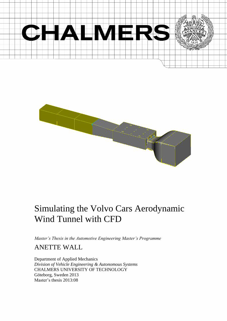
Cover:
CAD model representing the computational domain of the Volvo Car Aerodynamic
Wind Tunnel.
Chalmers Reproservice
Göteborg, Sweden 2013
CHALMERS, Applied Mechanics, Master’s Thesis 2013:08 V
Simulating the Volvo Car Aerodynamic Wind Tunnel with CFD
Master’s Thesis in the Automotive Engineering Master’s Programme
ANETTE WALL
Department of Applied Mechanics
Division of Vehicle Engineering & Autonomous Systems
Chalmers University of Technology
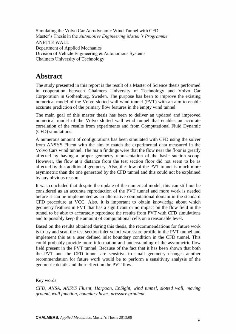
Abstract
The study presented in this report is the result of a Master of Science thesis performed
in cooperation between Chalmers University of Technology and Volvo Car
Corporation in Gothenburg, Sweden. The purpose has been to improve the existing
numerical model of the Volvo slotted wall wind tunnel (PVT) with an aim to enable
accurate prediction of the primary flow features in the empty wind tunnel.
The main goal of this master thesis has been to deliver an updated and improved
numerical model of the Volvo slotted wall wind tunnel that enables an accurate
correlation of the results from experiments and from Computational Fluid Dynamic
(CFD) simulations.
A numerous amount of configurations has been simulated with CFD using the solver
from ANSYS Fluent with the aim to match the experimental data measured in the
Volvo Cars wind tunnel. The main findings were that the flow near the floor is greatly
affected by having a proper geometry representation of the basic suction scoop.
However, the flow at a distance from the test section floor did not seem to be as
affected by this additional geometry. Also, the flow of the PVT tunnel is much more
asymmetric than the one generated by the CFD tunnel and this could not be explained
by any obvious reason.
It was concluded that despite the update of the numerical model, this can still not be
considered as an accurate reproduction of the PVT tunnel and more work is needed
before it can be implemented as an alternative computational domain in the standard
CFD procedure at VCC. Also, it is important to obtain knowledge about which
geometry features in PVT that has a significant or no impact on the flow field in the
tunnel to be able to accurately reproduce the results from PVT with CFD simulations
and to possibly keep the amount of computational cells on a reasonable level.
Based on the results obtained during this thesis, the recommendations for future work
is to try and scan the test section inlet velocity/pressure profile in the PVT tunnel and
implement this as a user defined inlet boundary condition in the CFD tunnel. This
could probably provide more information and understanding of the asymmetric flow
field present in the PVT tunnel. Because of the fact that it has been shown that both
the PVT and the CFD tunnel are sensitive to small geometry changes another
recommendation for future work would be to perform a sensitivity analysis of the
geometric details and their effect on the PVT flow.
Key words:
CFD, ANSA, ANSYS Fluent, Harpoon, EnSight, wind tunnel, slotted wall, moving
ground, wall function, boundary layer, pressure gradient

CHALMERS, Applied Mechanics, Master’s Thesis 2013:08 VI
CHALMERS, Applied Mechanics, Master’s Thesis 2013:08 VII
Table of contents
ABSTRACT V
TABLE OF CONTENTS VII
PREFACE/ACKNOWLEDGEMENTS XI
NOTATIONS XII
1 INTRODUCTION 1
1.1 Background 1
1.2 Objectives 2
1.3 Delimitations 2
1.4 Outline of the report 2
2 THEORY 3
2.1 The governing equations 3
2.2 Turbulence modelling 3
2.3 Near wall flow 4
2.3.1 Law of the wall 4 2.3.2 Wall functions 4
3 METHODOLOGY 7
3.1 The CFD process 7
3.1.1 Pre-processing 7 3.1.2 Solving 7
3.1.3 Post-processing 7
3.2 Physical wind tunnel testing 8
4 THE VOLVO CARS SLOTTED WALL WIND TUNNEL 11
4.1 The physical wind tunnel 11
4.2 The numerical wind tunnel setup 13 4.2.1 Computational domain and boundary conditions 13
4.2.2 Modelling boundary layer control systems 14
5 CALCULATION SETTINGS 17
5.1 Volume mesh 17 5.1.1 Prism layer 17 5.1.2 Velocity calculation and pressure coefficient evaluation 18
6 RESULTS 21
6.1 Flow field asymmetry 21
CHALMERS, Applied Mechanics, Master’s Thesis 2013:08 VIII
6.1.1 Pressure gradient at wall 21
6.2 Axial pressure gradient 23
6.3 Comparison of different wall functions 23
6.4 Experimental results vs CFD results 28
6.4.1 Pressure distribution in tunnel contraction 28 6.4.2 Pressure distribution along intermediate zone 29
7 DISCUSSION AND CONCLUSIONS 35
7.1 Discussion 35
7.2 Conclusions 36
8 RECOMMENDATIONS FOR FUTURE WORK 37
9 REFERENCES 39
APPENDIX A – HARPOON CONFIGURATION FILE I
APPENDIX B – FLUENT SETTINGS FILE V
APPENDIX C – FLUENT RUN FILE VII
APPENDIX D – ENSIGHT POST PROCESSING FILE XI
TABLE OF FIGURES
Figure 1 Standard computational domain at VCC representing a wind tunnel. ............ 1
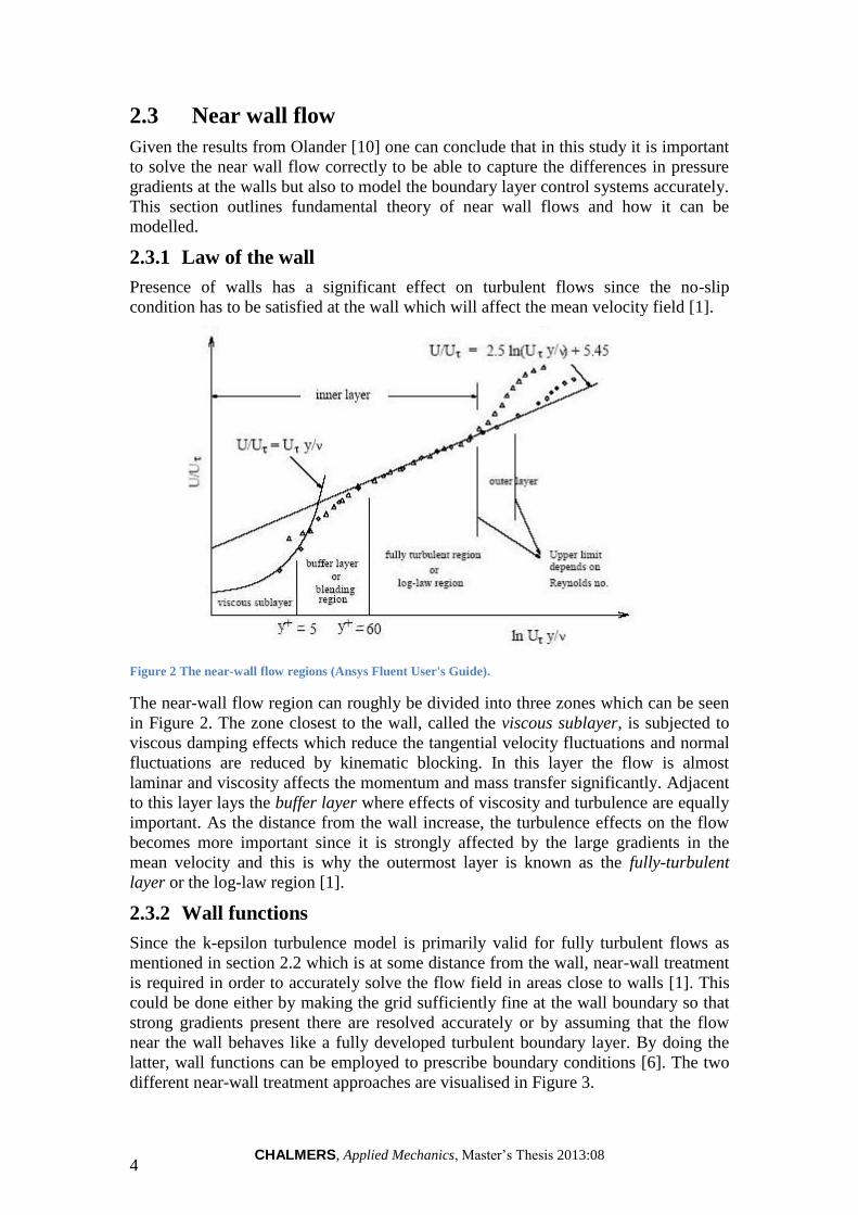
Figure 2 The near-wall flow regions (Ansys Fluent User's Guide). .............................. 4
Figure 3 Near-wall treatment approaches. Left: Wall function approach. Right: Fine
grid approach [1]. ........................................................................................................... 5
Figure 4 Pressure measurement probes mounted in nozzle ceiling. Picture taken
toward the flow direction. .............................................................................................. 8
Figure 5 Pressure measurement probes mounted in nozzle floor and along the
intermediate zone of the test section floor. .................................................................... 9
Figure 6 Schematic of the Prandtl tube used in experimental measurements [15]. ....... 9
Figure 7 Schematic of the closed air path of the Volvo Cars aerodynamic wind tunnel
[courtesy of Volvo Cars]. ............................................................................................. 11
Figure 8 The test section including the slotted walls and scale situated under the floor.
...................................................................................................................................... 12
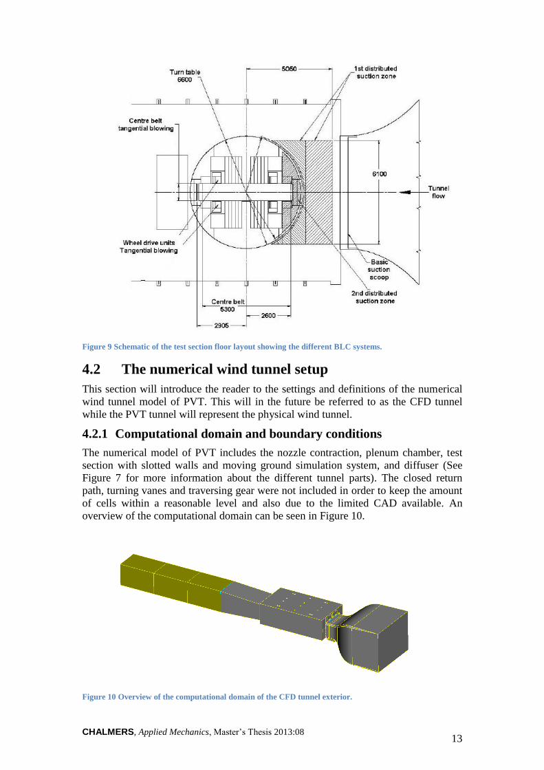
Figure 9 Schematic of the test section floor layout showing the different BLC
systems. ........................................................................................................................ 13
Figure 10 Overview of the computational domain of the CFD tunnel exterior. .......... 13
CHALMERS, Applied Mechanics, Master’s Thesis 2013:08 IX
Figure 11 The slotted wall test section exterior. .......................................................... 14
Figure 12 The test section floor layout as it is modelled in the CFD tunnel. .............. 15
Figure 13 3D geometry of the basic suction scoop- .................................................... 15
Figure 14 Test section plenum with the flow reinjection areas represented by the
yellow PIDs on in the front wall of the plenum. .......................................................... 16
Figure 15 Section cut of the volume mesh generated in Harpoon. .............................. 17
Figure 16 Zoomed in view of the prism layers added to the test section floor. ........... 17
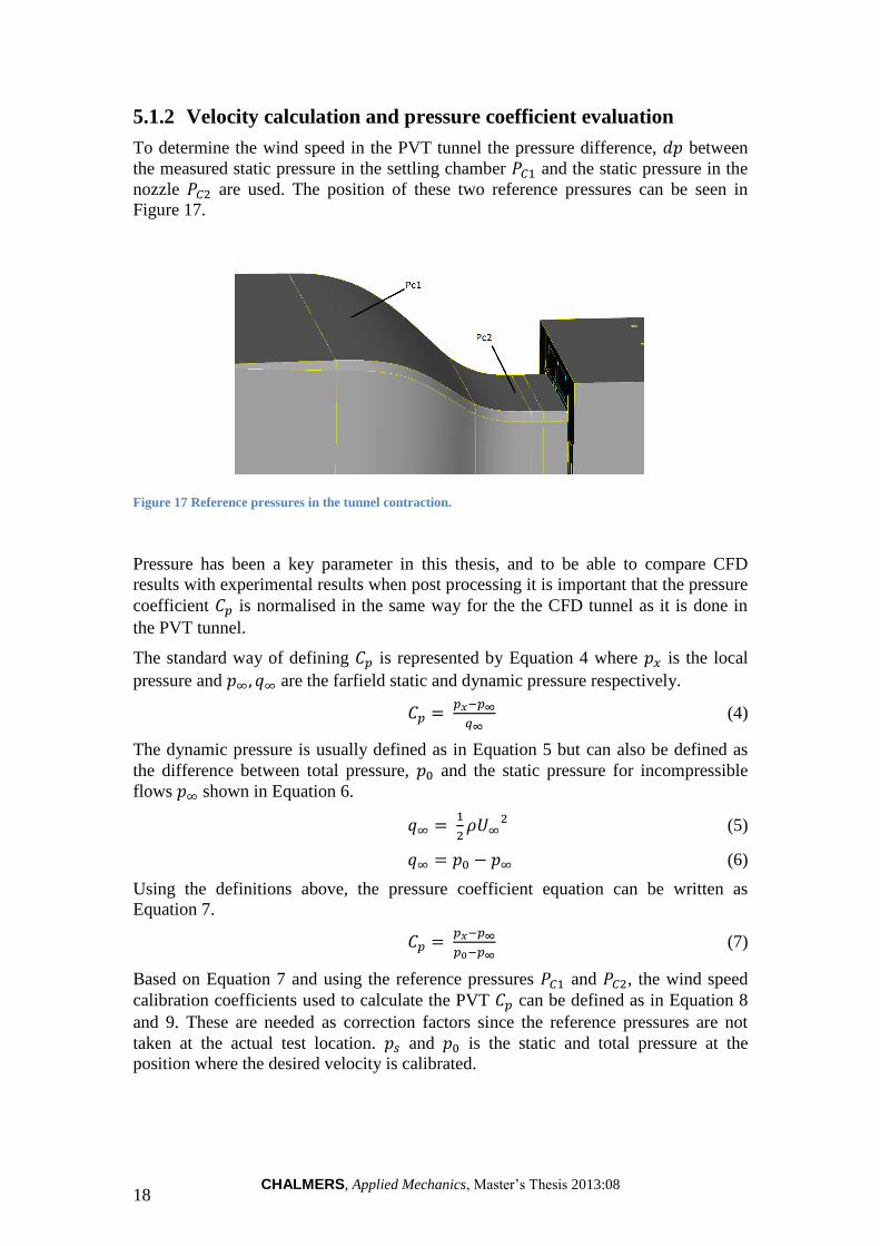
Figure 17 Reference pressures in the tunnel contraction. ............................................ 18
Figure 18 Pressure distribution on the slotted walls. Left: Right side of the test
section. Right: Left side of the test section. ................................................................. 21
Figure 19 Pressure gradient obtained from CFD simulations at the wall along the 2nd
slot. ............................................................................................................................... 22
Figure 20 Pressure gradient at wall comparison between CFD and experimental
results. .......................................................................................................................... 22
Figure 21 Axial pressure gradient comparison between CFD and experimental results.
...................................................................................................................................... 23
Figure 22 Axial pressure gradient from CFD employing different wall functions. ..... 24
Figure 23 Pressure gradient at wall from CFD employing different wall functions. .. 25
Figure 24 Boundary layer formation along centreline employing different wall
functions. Top: Standard. Middle: Non-Equilibrium. Bottom: Enhanced. .................. 26
Figure 25 Section cut of the test section entrance employing different wall functions.
Top: Standard. Middle: Non-Equilibrium. Bottom: Enhanced. ................................... 27
Figure 26 Measurement points in tunnel nozzle. ......................................................... 28
Figure 27 Pressure distribution on nozzle floor. .......................................................... 29
Figure 28 Pressure distribution on nozzle ceiling. ....................................................... 29
Figure 29 Pressure gradient along intermediate zone comparison between CFD and
experimental results from the first test conducted. ...................................................... 30
Figure 30 Pressure gradient along intermediate zone comparison between CFD and
experimental results from the second test conducted. ................................................. 30
Figure 31 Difference in pressure gradient in test section visualised by a pixel colour
comparison script. ........................................................................................................ 31
Figure 32 Difference in pressure gradient zoomed in at basic suction scoop area. ..... 32
Figure 33 Pressure gradient along the intermediate zone at different velocities during
a Reynolds sweep. ........................................................................................................ 32
Figure 34 Pressure gradient profile along the intermediate zone at different heights
above the floor. ............................................................................................................ 33
Figure 35 Pressure distribution above the intermediate zone. ..................................... 33

CHALMERS, Applied Mechanics, Master’s Thesis 2013:08 X
CHALMERS, Applied Mechanics, Master’s Thesis 2013:08 XI
Preface/Acknowledgements
This thesis was conducted as conclusion of the authors Master of Science degree at
the Mechanical Engineering program at Chalmers University of Technology. The
thesis work was performed at the Aerodynamics section, 91760 at Volvo Car
Corporation in Gothenburg during the spring of 2013. Supervisor of this thesis has
been Dr. Christoffer Landström, Analysis engineer at 91760 Aerodynamics section at
VCC and the examiner has been Professor Lennart Löfdahl at Chalmers University of
Technology.
I would like to start with acknowledge my supervisor Dr. Christoffer Landström for
being an excellent tutor, always taking his time to patiently answer all my questions
and in a pedagogical way explain things when needed.
A great thank you to my examiner Professor Lennart Löfdahl for the support not only
throughout the thesis, but also for the guidance and help in the transition from a
student into a career as an engineer.
Thanks to the people working at the section 91760 Aerodynamics for welcoming me
into their group and teach me about VCC. To technical expert Tim Walker for
providing extensive knowledge about PVT and to Dr. Simone Sebben for providing
valuable ideas and discussion regarding the CFD tunnel modelling. Also, to
Alexander Broniewicz for giving me the opportunity to be a part of the VESC
program including this thesis project.
A special thanks to the CFD family for bringing love, laughter and professional
support from day one at VCC.
The tunnel personnel for always pushing the limit to enable measurements that
seemed impossible to obtain and doing this in a professional manner during the
experimental testing in the Volvo Cars wind tunnel. Also mechanic Stefan Gribing for
the help preparing the test equipment.
Last but not least, I would like to thank my family and friends for the constant love
and support. Without you, this university journey would not have been possible.
Göteborg Juni 2013
Anette Wall
CHALMERS, Applied Mechanics, Master’s Thesis 2013:08 XII
Notations
pC Pressure coefficient
dp Pressure difference
pk VCC wind tunnel calibration coefficient
qk VCC wind tunnel calibration coefficient
1CP Static pressure in settling chamber
2CP Static pressure in nozzle
refP Static pressure at turntable centre at z=1200mm
y Dimensionless wall distance [-] *y Dimensionless wall distance used in Fluent [-]
BLCS Boundary Layer Control System
CAD Computer Aided Design
CFD Computational Fluid Dynamics
CFD tunnel Numerical model of PVT
GESS Ground Effect Simulation System
GUI Graphical User Interface
PID Property Identification
PVT Volvo Car Slotted Wall Wind Tunnel
RANS Reynold’s Averaged Navier Stokes
WDU Wheel Drive Unit
VCC Volvo Car Corporation
CHALMERS, Applied Mechanics, Master’s Thesis 2013:08 1
1 Introduction
This report has been written as a documentation of the work performed in this Master
Thesis that was requested by Volvo Cars Corporation (VCC) during the spring 2013.
This introduction chapter presents the background, objectives, delimitations and
outline of the report.
1.1 Background
Over the past years the accuracy of Computational Fluid Dynamic (CFD) results has
been greatly improved through better physical modelling together with the ability to
use more computational mesh cells and higher order numerical schemes. Although,
CFD results are still considered by many as a complement in the vehicle development
process and wind-tunnel results as the reference [5]. The trend in the automotive
industry is however to reduce the number of physical prototypes and in the future use
numerical models for vehicle verification. To enable this, modelling assumptions
must be reduced to a minimum [11]. According to [5] there are two possible ways of
generate an accurate comparison between CFD results and wind-tunnel results. One
way is to set up the CFD simulation for open road conditions and correct the wind-
tunnel results to take blockage effects into account. The other way is to reproduce the
exact physical wind-tunnel environment in the CFD setup, simulating also the moving
ground system as it is done in the physical wind-tunnel with moving belts and
boundary layer control systems [5].
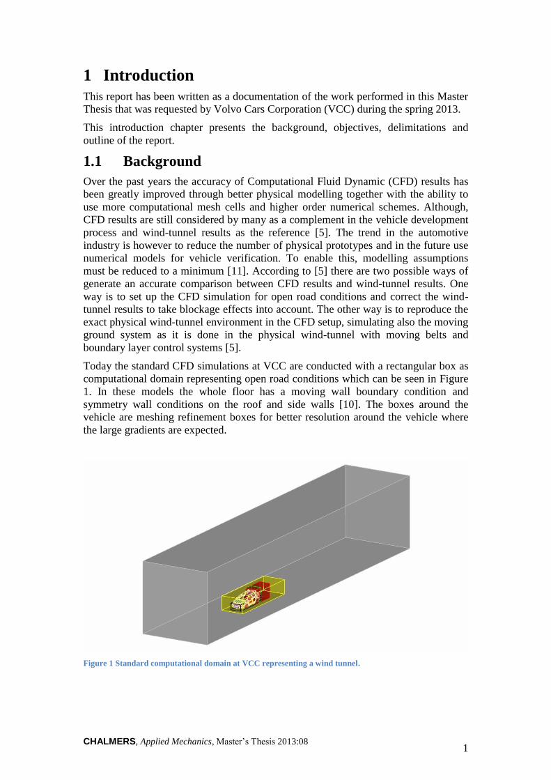
Today the standard CFD simulations at VCC are conducted with a rectangular box as
computational domain representing open road conditions which can be seen in Figure
1. In these models the whole floor has a moving wall boundary condition and
symmetry wall conditions on the roof and side walls [10]. The boxes around the
vehicle are meshing refinement boxes for better resolution around the vehicle where
the large gradients are expected.
Figure 1 Standard computational domain at VCC representing a wind tunnel.
CHALMERS, Applied Mechanics, Master’s Thesis 2013:08 2
At VCC it was decided to try and to reproduce the results from the physical wind-
tunnel as an alternative to the standard CFD simulations. In 2011 Olander [10]
performed a first attempt to generate a numerical model of the physical wind tunnel to
enable comparison between the results obtained from the experiments conducted in
PVT and the results from CFD simulations similar to the approach explained by Cyr
[5]. According to measurements performed in PVT by Eng [8] in 2009 a significant
difference in pressure distribution on the right side wall versus the left side was
discovered. The right side wall was subjected to two major pressure drops at the
support bars while the left side was not. This difference was also captured in the CFD
model but when compared to the experimental results the magnitude of the CFD
results were far from the experimental ones [10].
1.2 Objectives
The purpose of this master thesis is to improve the existing numerical model of the
Volvo slotted wall wind tunnel with an aim to enable accurate prediction of the
primary flow features in the empty wind tunnel including flow uniformity, static
pressure gradient, effect of ground simulation and interaction with the slotted walls
and surrounding support structures.
The main goal of this master thesis is to deliver an updated and improved numerical
model of the Volvo slotted wall wind tunnel that enables an accurate correlation of the
results from experiments and from CFD simulations.
1.3 Delimitations
This master thesis work has only focused on improving the existing numerical model
and to enable comparison to the results from CFD simulations with the simplified
wind tunnel, standard VCC CFD simulation processes has been followed.
Because of the limited time frame, the main focus has been on improving the empty
tunnel and make those results as close to the results from PVT as possible.
1.4 Outline of the report
This report is divided into 8 parts starting out with a theoretical framework explaining
some of the fundamental fluid dynamics and theory behind the computational fluid
dynamics used in this study. The Method chapter will introduce the reader to the work
procedure of this study and also briefly explain the standard CFD process and
software used at VCC. In the Volvo Slotted Wall Wind Tunnel chapter the physical
wind-tunnel environment and subsystems known as PVT in this report will be further
presented. This chapter will then be followed up by the Numerical model chapter,
introducing the reader to the CAD model geometry of the wind-tunnel, mesh and
simulation settings. In the Result chapter obtained and processed data will be
presented and then further discussed in the Discussion and Conclusion chapter. Lastly,
the report finishes off with recommendations for future work.
CHALMERS, Applied Mechanics, Master’s Thesis 2013:08 3
2 Theory
This chapter outlines the theory considered relevant for this project work, presenting
some fundamental fluid dynamics and theory behind numerical simulations.
2.1 The governing equations
The governing equations of fluid flow and heat transfer around a body are the
continuity equation, the momentum equation, and the energy equation [13]. When
dealing with road vehicle external aerodynamics , the general approach is to assume
incompressible and isothermal flow [2].The flow can be considered incompressible as
long as Ma < 0.3 [14] which requires a velocity of 100 m/s at sea level and it is
unlikely that the flow will reach this high velocity anywhere in the computational
domain. This means that the energy equation can be neglected and hence the
continuity equation (Equation 1) and momentum equation (Equation 2) can be written
on incompressible form, neglecting the density terms [14].
(1)
(2)
V and u denotes the fluid velocities, p is the pressure. ρ is the fluid density and μ
represents the dynamic viscosity. The steady-state Reynold’s Averaged Navier Stokes
(RANS) mean solutions are obtained using the k-epsilon realisable turbulence model.
RANS is an additional simplification where the governing equations (Equation 1 and
2) are time-averaged and thus the time term is neglected [13]. When solving these
equations the solver uses different numerical schemes. At VCC the standard is to use
the 1st order upwind scheme for initialisation and then 2
nd order upwind scheme for
the transport equations to minimise numerical diffusion. This is done because the 1st
order is more stable and can generate a more stable solution before introducing the
more accurate but less stable 2nd
order. Initialisation of the simulation means that one
provides an initial “guess” for the solution flow field so that the solving of the
transport equations has something to begin from. The pressure is however obtained
using a pressure interpolation scheme where the pressure is interpolated at the faces
using momentum equation coefficients [10].
(3)
2.2 Turbulence modelling
In this study a variant of the k-epsilon turbulence model has been used, the realisable
k-epsilon model. The standard k-epsilon turbulence model is a two-equation eddy
viscosity model that has been widely used in industrial flow simulations, mainly
because of its robustness, economy and reasonable accuracy for a wide range of
turbulent flows. However, this model is limited by the fact that it only is valid for
fully turbulent flows. To deal with this limitation, the realisable k-epsilon turbulence
model was developed with its benefits of providing better accuracy for flows
involving rotation, boundary layers under strong adverse pressure gradients,
separation and recirculation [1].
CHALMERS, Applied Mechanics, Master’s Thesis 2013:08 4
2.3 Near wall flow
Given the results from Olander [10] one can conclude that in this study it is important
to solve the near wall flow correctly to be able to capture the differences in pressure
gradients at the walls but also to model the boundary layer control systems accurately.
This section outlines fundamental theory of near wall flows and how it can be
modelled.
2.3.1 Law of the wall
Presence of walls has a significant effect on turbulent flows since the no-slip
condition has to be satisfied at the wall which will affect the mean velocity field [1].
Figure 2 The near-wall flow regions (Ansys Fluent User's Guide).
The near-wall flow region can roughly be divided into three zones which can be seen
in Figure 2. The zone closest to the wall, called the viscous sublayer, is subjected to
viscous damping effects which reduce the tangential velocity fluctuations and normal
fluctuations are reduced by kinematic blocking. In this layer the flow is almost
laminar and viscosity affects the momentum and mass transfer significantly. Adjacent
to this layer lays the buffer layer where effects of viscosity and turbulence are equally
important. As the distance from the wall increase, the turbulence effects on the flow
becomes more important since it is strongly affected by the large gradients in the
mean velocity and this is why the outermost layer is known as the fully-turbulent
layer or the log-law region [1].
2.3.2 Wall functions
Since the k-epsilon turbulence model is primarily valid for fully turbulent flows as
mentioned in section 2.2 which is at some distance from the wall, near-wall treatment
is required in order to accurately solve the flow field in areas close to walls [1]. This
could be done either by making the grid sufficiently fine at the wall boundary so that
strong gradients present there are resolved accurately or by assuming that the flow
near the wall behaves like a fully developed turbulent boundary layer. By doing the
latter, wall functions can be employed to prescribe boundary conditions [6]. The two
different near-wall treatment approaches are visualised in Figure 3.
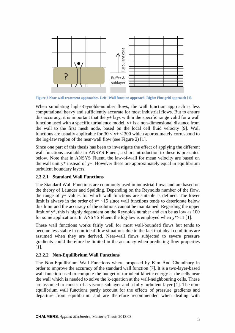
CHALMERS, Applied Mechanics, Master’s Thesis 2013:08 5
Figure 3 Near-wall treatment approaches. Left: Wall function approach. Right: Fine grid approach [1].
When simulating high-Reynolds-number flows, the wall function approach is less
computational heavy and sufficiently accurate for most industrial flows. But to ensure
this accuracy, it is important that the y+ lays within the specific range valid for a wall
function used with a specific turbulence model. y+ is a non-dimensional distance from
the wall to the first mesh node, based on the local cell fluid velocity [9]. Wall
functions are usually applicable for 30 < y+ < 300 which approximately correspond to
the log-law region of the near-wall flow (see Figure 2) [1].
Since one part of this thesis has been to investigate the effect of applying the different
wall functions available in ANSYS Fluent, a short introduction to these is presented
below. Note that in ANSYS Fluent, the law-of-wall for mean velocity are based on
the wall unit y* instead of y+. However these are approximately equal in equilibrium
turbulent boundary layers.
2.3.2.1 Standard Wall Functions
The Standard Wall Functions are commonly used in industrial flows and are based on
the theory of Launder and Spalding. Depending on the Reynolds number of the flow,
the range of y+ values for which wall functions are suitable is defined. The lower
limit is always in the order of y* ~15 since wall functions tends to deteriorate below
this limit and the accuracy of the solutions cannot be maintained. Regarding the upper
limit of y*, this is highly dependent on the Reynolds number and can be as low as 100
for some applications. In ANSYS Fluent the log-law is employed when y*>11 [1].
These wall functions works fairly well for most wall-bounded flows but tends to
become less stable in non-ideal flow situations due to the fact that ideal conditions are
assumed when they are derived. Near-wall flows subjected to severe pressure
gradients could therefore be limited in the accuracy when predicting flow properties
[1].
2.3.2.2 Non-Equilibrium Wall Functions
The Non-Equilibrium Wall Functions where proposed by Kim And Choudhury in
order to improve the accuracy of the standard wall function [7]. It is a two-layer-based
wall function used to compute the budget of turbulent kinetic energy at the cells near
the wall which is needed to solve the k-equation at the wall-neighbouring cells. These
are assumed to consist of a viscous sublayer and a fully turbulent layer [1]. The non-
equilibrium wall functions partly account for the effects of pressure gradients and
departure from equilibrium and are therefore recommended when dealing with
CHALMERS, Applied Mechanics, Master’s Thesis 2013:08 6
complex flows involving separation, reattachment, and when mean flow and
turbulence are subjected to severe pressure gradients and change rapidly [7].
2.3.2.3 Enhanced Wall Functions
It is desirable to have a near-wall formulation that can be used for coarse meshes
(wall-function meshes) as well as fine meshes (low-Reynolds-number meshes).
Furthermore, intermediate meshes where the first near-wall node is placed neither in
the fully turbulent regions, where the wall functions are suitable, nor in the direct
vicinity of the wall at y+=~1, where the low-Reynold-number approach is suitable,
should not generate excessive error. These wall functions are based on the action of
combining a two-layer model with so-called enhanced wall functions. This means that
if the near-wall mesh is fine enough to be able to resolve the viscous sublayer
(y+=~1), the enhanced wall treatment will be identical to the traditional two-layer
zonal model [1].
CHALMERS, Applied Mechanics, Master’s Thesis 2013:08 7
3 Methodology
In this study an alternative computational domain for road vehicle simulations at VCC
has been analysed. Since the initial study was performed by Olander [10] the
methodology of this work naturally started with a literature study of the report from
that work but also other reports and papers related to the subject. The main part of this
study could be identified as an iterative process using the standard CFD tools at VCC
and continuously comparing the results obtained from these to experimental results to
achieve the goal stated in Section 1.2.
3.1 The CFD process
Since the CFD process has been the core of this study, this will be further explained
and the software used introduced in this subsection. The CFD process can be divided
into three steps; pre-processing, solving and post-processing.
3.1.1 Pre-processing
In order to be able to use a CAD model for flow simulations, the first step is to reduce
the level of detail so that only the surfaces that will have a possible impact on the flow
are left. This is done in order to decrease the amount of cells and hence reduce the
simulation time. This will also enable better mesh quality. However, in such a case
that has been dealt with in this thesis where it has been shown that different geometry
changes affects the flow in the tunnel more or less significantly, it is important to
remove details with care and be sure that they do not influence the flow in the tunnel.
The CAD-cleanup of the PVT CFD wind tunnel model was done prior to this study
and the software used for this was ANSA from BETA CAE Systems. ANSA has been
used in this study to generate an initial surface mesh consisting of triangles of
different size depending on the geometry shape. In important areas, for example
where large pressure gradients are expected, in this study the resolution was set to a
finer level.
The surface mesh generated by ANSA was then exported to another software,
Harpoon, for volume meshing. To better resolve the flow near the walls, a prism layer
was applied to the solid walls in the test section area. More information about this can
be found in Section 5.1.
3.1.2 Solving
After pre-processing the model, the computational mesh that was generated was
imported into the solver software. In this study numerical simulations were performed
using ANSYS Fluent 13.0.2 with an aim of reproducing the experimental works by
Bender [3] or Eng [8]. As mentioned earlier in the Theory chapter, the solver used for
this thesis is a RANS (Reynolds Averaged Navier Stokes) steady state solver
employing the k-epsilon realisable turbulence model. In the solver all boundary
conditions and solver settings where specified before initialising the solution. The
boundary conditions will be further specified in Section 4.2. For the near wall flow,
wall functions have been employed as described in the previous chapter. 1st order
upwind discretisation scheme was used for initialisation of the solution and 2nd
order
for solving of the momentum equations.
3.1.3 Post-processing
After finalising a simulation, the physical quantities where exported to a post-
processing software to enable visualisation of the results. In this study EnSight from
CHALMERS, Applied Mechanics, Master’s Thesis 2013:08 8
CEI Software was used for graphical post-processing. The results could be displayed
in many different ways and in this study the most interesting parameters to visualise
were pressure and velocity distribution. Some data was also exported to MS Excel and
MATLAB from MathWorks to be able to compare with experimental data.
3.2 Physical wind tunnel testing
For better understanding of the measurement locations described in this section, the
reader should be advised to see Chapter 4 for more information about the different
geometries of the Volvo Car aerodynamic wind tunnel. The experimental testing
performed in this thesis has been conducted in this wind tunnel mainly focusing on
obtaining input of the pressure distribution in the tunnel contraction and test section
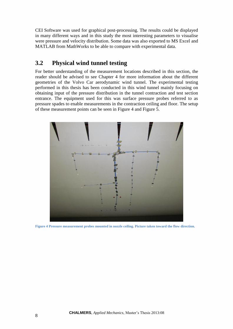
entrance. The equipment used for this was surface pressure probes referred to as
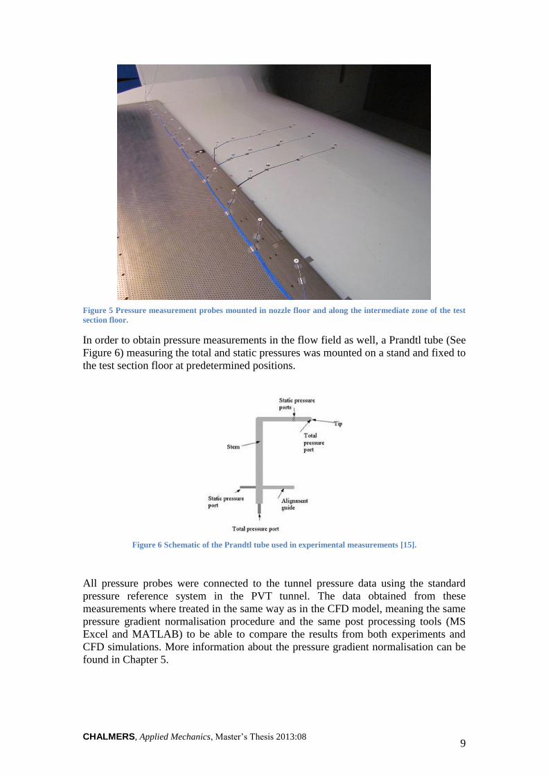
pressure spades to enable measurements in the contraction ceiling and floor. The setup
of these measurement points can be seen in Figure 4 and Figure 5.
Figure 4 Pressure measurement probes mounted in nozzle ceiling. Picture taken toward the flow direction.
CHALMERS, Applied Mechanics, Master’s Thesis 2013:08 9
Figure 5 Pressure measurement probes mounted in nozzle floor and along the intermediate zone of the test
section floor.
In order to obtain pressure measurements in the flow field as well, a Prandtl tube (See
Figure 6) measuring the total and static pressures was mounted on a stand and fixed to
the test section floor at predetermined positions.
Figure 6 Schematic of the Prandtl tube used in experimental measurements [15].
All pressure probes were connected to the tunnel pressure data using the standard
pressure reference system in the PVT tunnel. The data obtained from these
measurements where treated in the same way as in the CFD model, meaning the same
pressure gradient normalisation procedure and the same post processing tools (MS
Excel and MATLAB) to be able to compare the results from both experiments and
CFD simulations. More information about the pressure gradient normalisation can be
found in Chapter 5.

CHALMERS, Applied Mechanics, Master’s Thesis 2013:08 10
CHALMERS, Applied Mechanics, Master’s Thesis 2013:08 11
4 The Volvo Cars slotted wall wind tunnel
This chapter has been divided into two main sections where the first one presents the
physical Volvo Cars aerodynamic wind tunnel and the second part presents the
numerical CFD model that was developed by Olander in 2011.
4.1 The physical wind tunnel
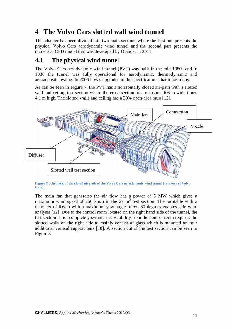
The Volvo Cars aerodynamic wind tunnel (PVT) was built in the mid-1980s and in
1986 the tunnel was fully operational for aerodynamic, thermodynamic and
aeroacoustic testing. In 2006 it was upgraded to the specifications that it has today.
As can be seen in Figure 7, the PVT has a horizontally closed air-path with a slotted
wall and ceiling test section where the cross section area measures 6.6 m wide times
4.1 m high. The slotted walls and ceiling has a 30% open-area ratio [12].
Figure 7 Schematic of the closed air path of the Volvo Cars aerodynamic wind tunnel [courtesy of Volvo
Cars].
The main fan that generates the air flow has a power of 5 MW which gives a
maximum wind speed of 250 km/h in the 27 m2 test section. The turntable with a
diameter of 6.6 m with a maximum yaw angle of +/- 30 degrees enables side wind
analysis [12]. Due to the control room located on the right hand side of the tunnel, the
test section is not completely symmetric. Visibility from the control room requires the
slotted walls on the right side to mainly consist of glass which is mounted on four
additional vertical support bars [10]. A section cut of the test section can be seen in
Figure 8.
Main fan
Nozzle
Contraction
Slotted wall test section
Diffuser
CHALMERS, Applied Mechanics, Master’s Thesis 2013:08 12
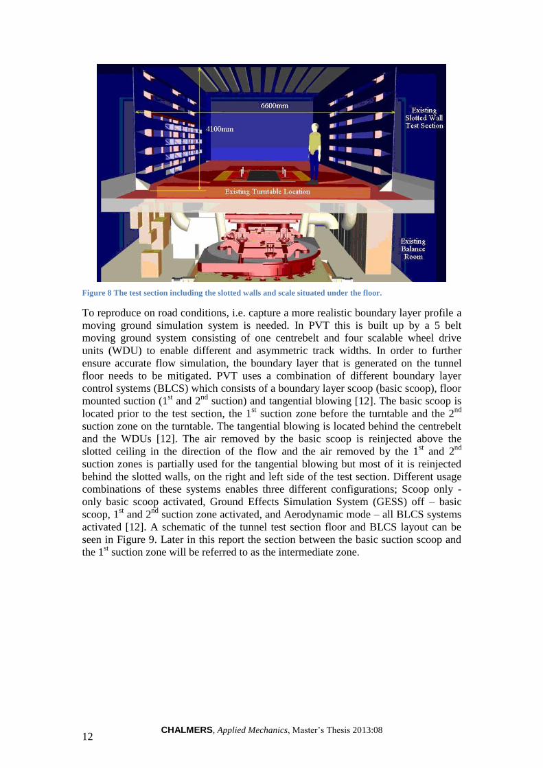
Figure 8 The test section including the slotted walls and scale situated under the floor.
To reproduce on road conditions, i.e. capture a more realistic boundary layer profile a
moving ground simulation system is needed. In PVT this is built up by a 5 belt
moving ground system consisting of one centrebelt and four scalable wheel drive
units (WDU) to enable different and asymmetric track widths. In order to further
ensure accurate flow simulation, the boundary layer that is generated on the tunnel
floor needs to be mitigated. PVT uses a combination of different boundary layer
control systems (BLCS) which consists of a boundary layer scoop (basic scoop), floor
mounted suction (1st and 2
nd suction) and tangential blowing [12]. The basic scoop is
located prior to the test section, the 1st suction zone before the turntable and the 2
nd
suction zone on the turntable. The tangential blowing is located behind the centrebelt
and the WDUs [12]. The air removed by the basic scoop is reinjected above the
slotted ceiling in the direction of the flow and the air removed by the 1st and 2
nd
suction zones is partially used for the tangential blowing but most of it is reinjected
behind the slotted walls, on the right and left side of the test section. Different usage
combinations of these systems enables three different configurations; Scoop only -
only basic scoop activated, Ground Effects Simulation System (GESS) off – basic
scoop, 1st and 2
nd suction zone activated, and Aerodynamic mode – all BLCS systems
activated [12]. A schematic of the tunnel test section floor and BLCS layout can be
seen in Figure 9. Later in this report the section between the basic suction scoop and
the 1st suction zone will be referred to as the intermediate zone.
CHALMERS, Applied Mechanics, Master’s Thesis 2013:08 13
Figure 9 Schematic of the test section floor layout showing the different BLC systems.
4.2 The numerical wind tunnel setup
This section will introduce the reader to the settings and definitions of the numerical
wind tunnel model of PVT. This will in the future be referred to as the CFD tunnel
while the PVT tunnel will represent the physical wind tunnel.
4.2.1 Computational domain and boundary conditions
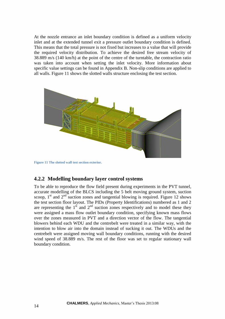
The numerical model of PVT includes the nozzle contraction, plenum chamber, test
section with slotted walls and moving ground simulation system, and diffuser (See
Figure 7 for more information about the different tunnel parts). The closed return
path, turning vanes and traversing gear were not included in order to keep the amount
of cells within a reasonable level and also due to the limited CAD available. An
overview of the computational domain can be seen in Figure 10.
Figure 10 Overview of the computational domain of the CFD tunnel exterior.
CHALMERS, Applied Mechanics, Master’s Thesis 2013:08 14
At the nozzle entrance an inlet boundary condition is defined as a uniform velocity
inlet and at the extended tunnel exit a pressure outlet boundary condition is defined.
This means that the total pressure is not fixed but increases to a value that will provide
the required velocity distribution. To achieve the desired free stream velocity of
38.889 m/s (140 km/h) at the point of the centre of the turntable, the contraction ratio
was taken into account when setting the inlet velocity. More information about
specific value settings can be found in Appendix B. Non-slip conditions are applied to
all walls. Figure 11 shows the slotted walls structure enclosing the test section.
Figure 11 The slotted wall test section exterior.
4.2.2 Modelling boundary layer control systems
To be able to reproduce the flow field present during experiments in the PVT tunnel,
accurate modelling of the BLCS including the 5 belt moving ground system, suction
scoop, 1st and 2
nd suction zones and tangential blowing is required. Figure 12 shows
the test section floor layout. The PIDs (Property Identifications) numbered as 1 and 2
are representing the 1st and 2
nd suction zones respectively and to model these they
were assigned a mass flow outlet boundary condition, specifying known mass flows
over the zones measured in PVT and a direction vector of the flow. The tangential
blowers behind each WDU and the centrebelt were treated in a similar way, with the
intention to blow air into the domain instead of sucking it out. The WDUs and the
centrebelt were assigned moving wall boundary conditions, running with the desired
wind speed of 38.889 m/s. The rest of the floor was set to regular stationary wall
boundary condition.

CHALMERS, Applied Mechanics, Master’s Thesis 2013:08 15
Figure 12 The test section floor layout as it is modelled in the CFD tunnel.
The basic suction scoop geometry can be seen in Figure 13. The PID numbered as 3
representing the outlet of the scoop was set to a massflow inlet with a direction vector
similar to the suction zones and tangential blowers.
Figure 13 3D geometry of the basic suction scoop-
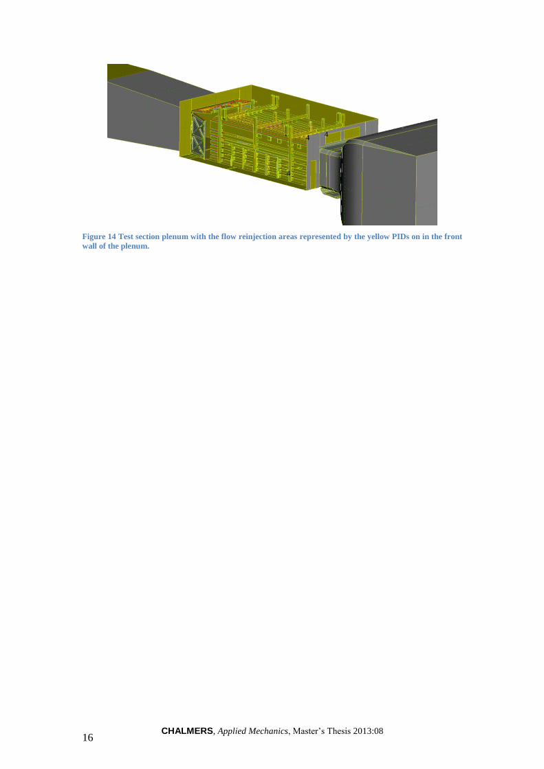
As described in Chapter 4, the air removed from the test section must be reinjected
somewhere. This is done by assigning mass flow inlets on the test section plenum
short side, partly on the sides and partly above the slotted walls. These inlets are
represented by the PIDs numbered as 4 in Figure 14.
1 2
3
CHALMERS, Applied Mechanics, Master’s Thesis 2013:08 16
Figure 14 Test section plenum with the flow reinjection areas represented by the yellow PIDs on in the front
wall of the plenum.
4 4
4
CHALMERS, Applied Mechanics, Master’s Thesis 2013:08 17
5 Calculation settings
This chapter outlines the results from the pre-processing, including presentation of the
mesh and velocity calibration.
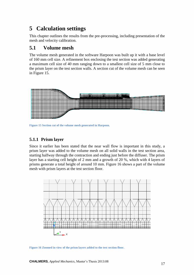
5.1 Volume mesh
The volume mesh generated in the software Harpoon was built up it with a base level
of 160 mm cell size. A refinement box enclosing the test section was added generating
a maximum cell size of 40 mm ranging down to a smallest cell size of 5 mm close to
the prism layer on the test section walls. A section cut of the volume mesh can be seen
in Figure 15.
Figure 15 Section cut of the volume mesh generated in Harpoon.
5.1.1 Prism layer
Since it earlier has been stated that the near wall flow is important in this study, a
prism layer was added to the volume mesh on all solid walls in the test section area,
starting halfway through the contraction and ending just before the diffuser. The prism
layer has a starting cell height of 2 mm and a growth of 20 %, which with 4 layers of
prisms generate a total height of around 10 mm. Figure 16 shows a part of the volume
mesh with prism layers at the test section floor.
Figure 16 Zoomed in view of the prism layers added to the test section floor.
CHALMERS, Applied Mechanics, Master’s Thesis 2013:08 18
5.1.2 Velocity calculation and pressure coefficient evaluation
To determine the wind speed in the PVT tunnel the pressure difference, between
the measured static pressure in the settling chamber and the static pressure in the
nozzle are used. The position of these two reference pressures can be seen in
Figure 17.
Figure 17 Reference pressures in the tunnel contraction.
Pressure has been a key parameter in this thesis, and to be able to compare CFD
results with experimental results when post processing it is important that the pressure
coefficient is normalised in the same way for the the CFD tunnel as it is done in
the PVT tunnel.
The standard way of defining is represented by Equation 4 where is the local
pressure and are the farfield static and dynamic pressure respectively.
(4)
The dynamic pressure is usually defined as in Equation 5 but can also be defined as
the difference between total pressure, and the static pressure for incompressible
flows shown in Equation 6.
(5)
(6)
Using the definitions above, the pressure coefficient equation can be written as
Equation 7.
(7)
Based on Equation 7 and using the reference pressures and , the wind speed
calibration coefficients used to calculate the PVT can be defined as in Equation 8
and 9. These are needed as correction factors since the reference pressures are not
taken at the actual test location. and is the static and total pressure at the
position where the desired velocity is calibrated.
CHALMERS, Applied Mechanics, Master’s Thesis 2013:08 19
(8)
(9)
Now the the PVT equation can be defined according to Equation 10.
(10)

CHALMERS, Applied Mechanics, Master’s Thesis 2013:08 20
CHALMERS, Applied Mechanics, Master’s Thesis 2013:08 21
6 Results
This chapter outlines the results obtained from the CFD simulations performed in this
study and how they correlate with experimental results from PVT.
6.1 Flow field asymmetry
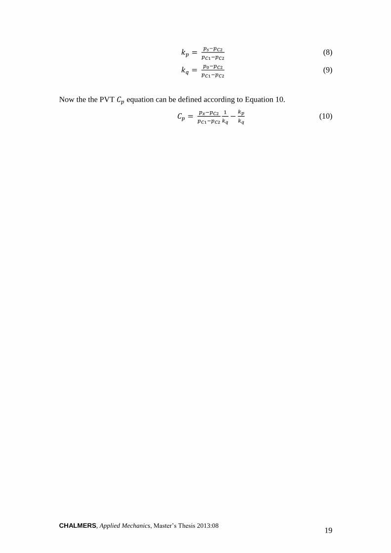
From the pressure measurements performed by Eng [8] in 2009 it is known that there
is a difference in pressure distribution on the slotted walls right and left side. This can
also be seen in the CFD results looking at Figure 18 where pressure has been plotted
on the right and left walls respectively. At the right side there are pressure drops at the
extra support bars described in Section 4.1 which is not present on the left wall.
Figure 18 Pressure distribution on the slotted walls. Left: Right side of the test section. Right: Left side of
the test section.
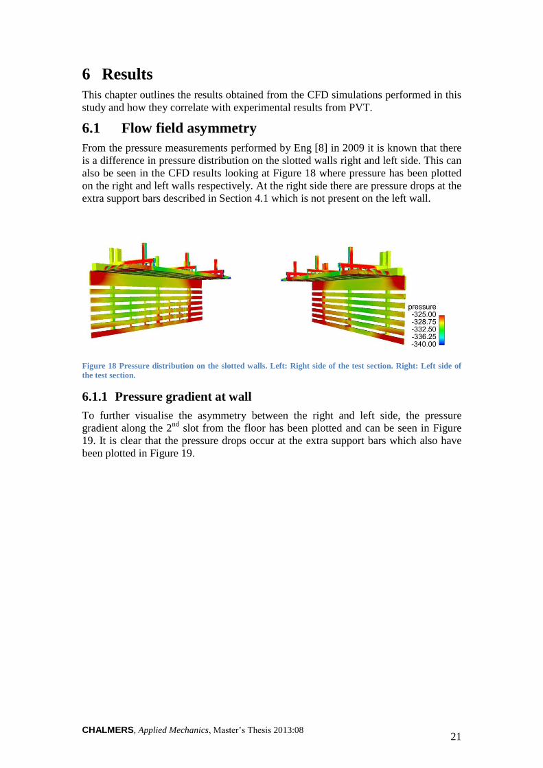
6.1.1 Pressure gradient at wall
To further visualise the asymmetry between the right and left side, the pressure
gradient along the 2nd
slot from the floor has been plotted and can be seen in Figure
19. It is clear that the pressure drops occur at the extra support bars which also have
been plotted in Figure 19.
CHALMERS, Applied Mechanics, Master’s Thesis 2013:08 22
Figure 19 Pressure gradient obtained from CFD simulations at the wall along the 2nd slot.
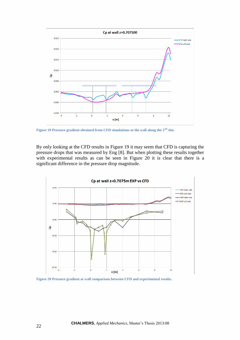
By only looking at the CFD results in Figure 19 it may seem that CFD is capturing the
pressure drops that was measured by Eng [8]. But when plotting these results together
with experimental results as can be seen in Figure 20 it is clear that there is a
significant difference in the pressure drop magnitude.
Figure 20 Pressure gradient at wall comparison between CFD and experimental results.
CHALMERS, Applied Mechanics, Master’s Thesis 2013:08 23
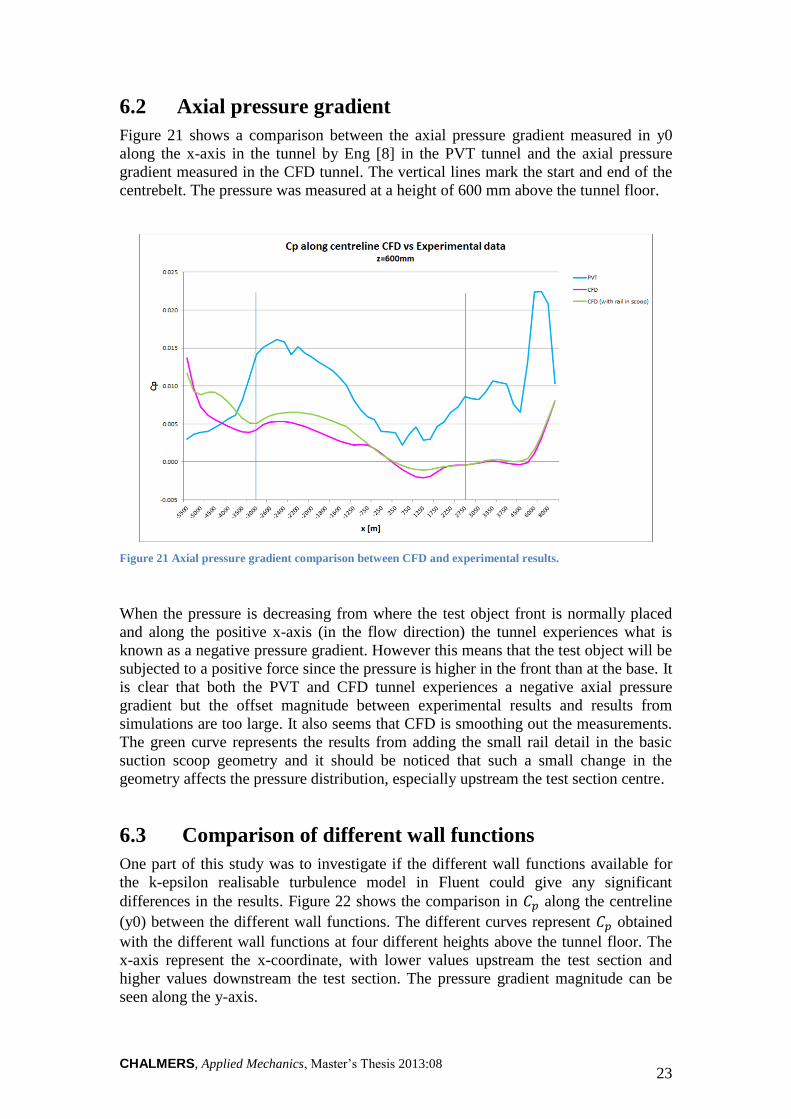
6.2 Axial pressure gradient
Figure 21 shows a comparison between the axial pressure gradient measured in y0
along the x-axis in the tunnel by Eng [8] in the PVT tunnel and the axial pressure
gradient measured in the CFD tunnel. The vertical lines mark the start and end of the
centrebelt. The pressure was measured at a height of 600 mm above the tunnel floor.
Figure 21 Axial pressure gradient comparison between CFD and experimental results.
When the pressure is decreasing from where the test object front is normally placed
and along the positive x-axis (in the flow direction) the tunnel experiences what is
known as a negative pressure gradient. However this means that the test object will be
subjected to a positive force since the pressure is higher in the front than at the base. It
is clear that both the PVT and CFD tunnel experiences a negative axial pressure
gradient but the offset magnitude between experimental results and results from
simulations are too large. It also seems that CFD is smoothing out the measurements.
The green curve represents the results from adding the small rail detail in the basic
suction scoop geometry and it should be noticed that such a small change in the
geometry affects the pressure distribution, especially upstream the test section centre.
6.3 Comparison of different wall functions
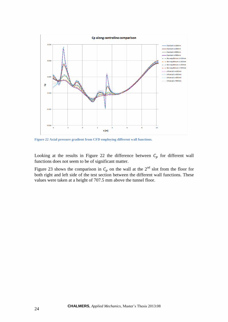
One part of this study was to investigate if the different wall functions available for
the k-epsilon realisable turbulence model in Fluent could give any significant
differences in the results. Figure 22 shows the comparison in along the centreline
(y0) between the different wall functions. The different curves represent obtained
with the different wall functions at four different heights above the tunnel floor. The
x-axis represent the x-coordinate, with lower values upstream the test section and
higher values downstream the test section. The pressure gradient magnitude can be
seen along the y-axis.
CHALMERS, Applied Mechanics, Master’s Thesis 2013:08 24
Figure 22 Axial pressure gradient from CFD employing different wall functions.
Looking at the results in Figure 22 the difference between for different wall
functions does not seem to be of significant matter.
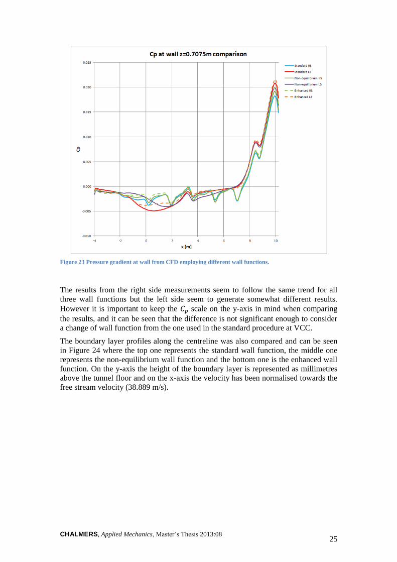
Figure 23 shows the comparison in on the wall at the 2nd
slot from the floor for
both right and left side of the test section between the different wall functions. These
values were taken at a height of 707.5 mm above the tunnel floor.
CHALMERS, Applied Mechanics, Master’s Thesis 2013:08 25
Figure 23 Pressure gradient at wall from CFD employing different wall functions.
The results from the right side measurements seem to follow the same trend for all
three wall functions but the left side seem to generate somewhat different results.
However it is important to keep the scale on the y-axis in mind when comparing
the results, and it can be seen that the difference is not significant enough to consider
a change of wall function from the one used in the standard procedure at VCC.
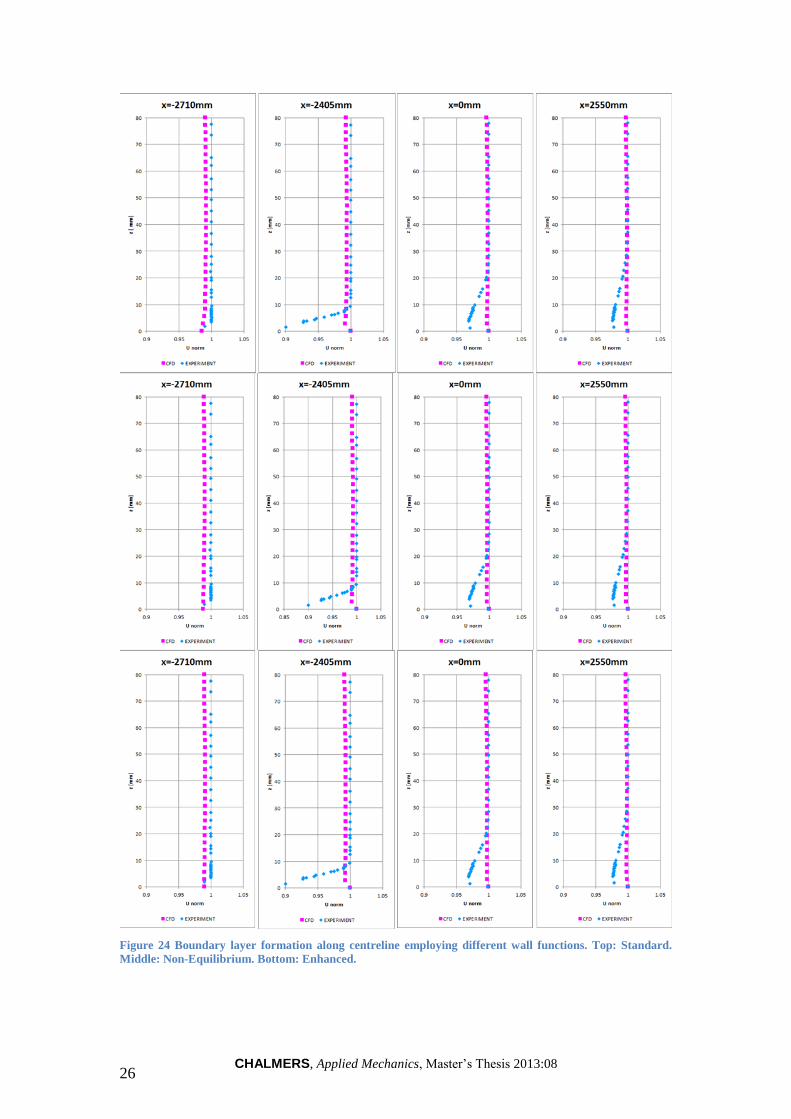
The boundary layer profiles along the centreline was also compared and can be seen
in Figure 24 where the top one represents the standard wall function, the middle one
represents the non-equilibrium wall function and the bottom one is the enhanced wall
function. On the y-axis the height of the boundary layer is represented as millimetres
above the tunnel floor and on the x-axis the velocity has been normalised towards the
free stream velocity (38.889 m/s).
CHALMERS, Applied Mechanics, Master’s Thesis 2013:08 26
Figure 24 Boundary layer formation along centreline employing different wall functions. Top: Standard.
Middle: Non-Equilibrium. Bottom: Enhanced.
CHALMERS, Applied Mechanics, Master’s Thesis 2013:08 27
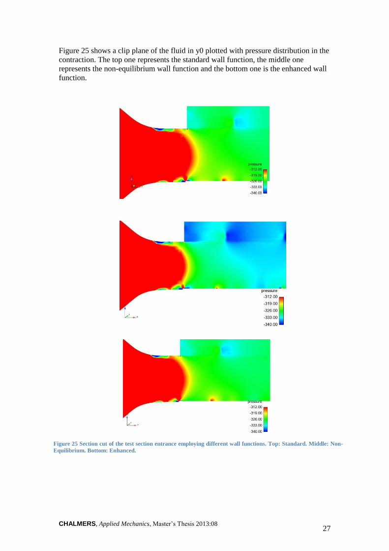
Figure 25 shows a clip plane of the fluid in y0 plotted with pressure distribution in the
contraction. The top one represents the standard wall function, the middle one
represents the non-equilibrium wall function and the bottom one is the enhanced wall
function.
Figure 25 Section cut of the test section entrance employing different wall functions. Top: Standard. Middle: Non-
Equilibrium. Bottom: Enhanced.
CHALMERS, Applied Mechanics, Master’s Thesis 2013:08 28
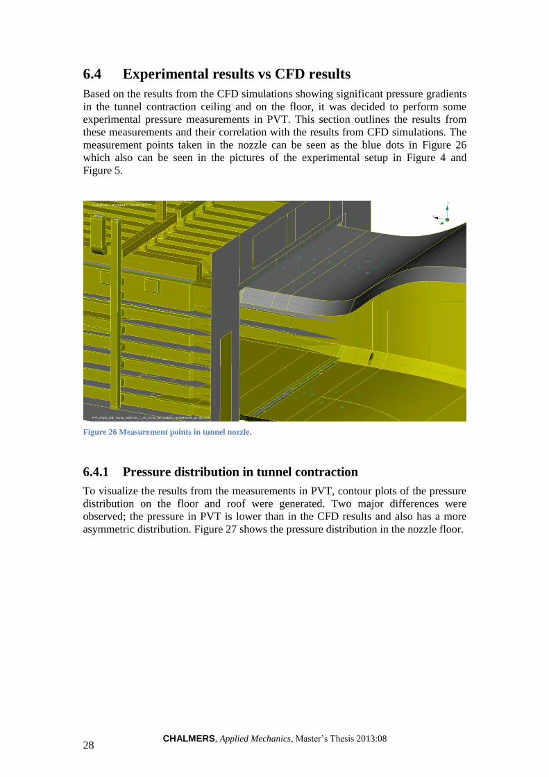
6.4 Experimental results vs CFD results
Based on the results from the CFD simulations showing significant pressure gradients
in the tunnel contraction ceiling and on the floor, it was decided to perform some
experimental pressure measurements in PVT. This section outlines the results from
these measurements and their correlation with the results from CFD simulations. The
measurement points taken in the nozzle can be seen as the blue dots in Figure 26
which also can be seen in the pictures of the experimental setup in Figure 4 and
Figure 5.
Figure 26 Measurement points in tunnel nozzle.
6.4.1 Pressure distribution in tunnel contraction
To visualize the results from the measurements in PVT, contour plots of the pressure
distribution on the floor and roof were generated. Two major differences were
observed; the pressure in PVT is lower than in the CFD results and also has a more
asymmetric distribution. Figure 27 shows the pressure distribution in the nozzle floor.
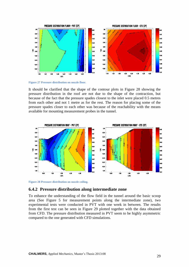
CHALMERS, Applied Mechanics, Master’s Thesis 2013:08 29
Figure 27 Pressure distribution on nozzle floor.
It should be clarified that the shape of the contour plots in Figure 28 showing the
pressure distribution in the roof are not due to the shape of the contraction, but
because of the fact that the pressure spades closest to the inlet were placed 0.5 metres
from each other and not 1 metre as for the rest. The reason for placing some of the
pressure spades closer to each other was because of the reachability with the means
available for mounting measurement probes in the tunnel.
Figure 28 Pressure distribution on nozzle ceiling.
6.4.2 Pressure distribution along intermediate zone
To enhance the understanding of the flow field in the tunnel around the basic scoop
area (See Figure 5 for measurement points along the intermediate zone), two
experimental tests were conducted in PVT with one week in between. The results
from the first test can be seen in Figure 29 plotted together with the data obtained
from CFD. The pressure distribution measured in PVT seem to be highly asymmetric
compared to the one generated with CFD simulations.
CHALMERS, Applied Mechanics, Master’s Thesis 2013:08 30
Figure 29 Pressure gradient along intermediate zone comparison between CFD and experimental results
from the first test conducted.
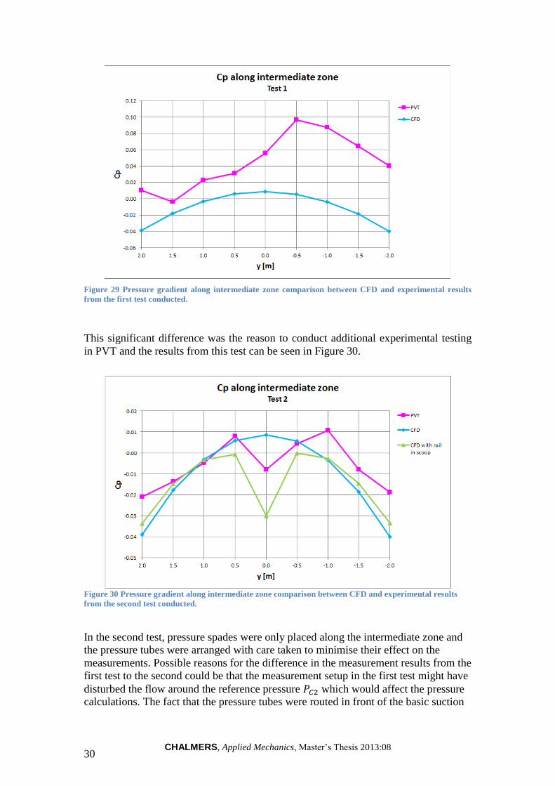
This significant difference was the reason to conduct additional experimental testing
in PVT and the results from this test can be seen in Figure 30.
Figure 30 Pressure gradient along intermediate zone comparison between CFD and experimental results
from the second test conducted.
In the second test, pressure spades were only placed along the intermediate zone and
the pressure tubes were arranged with care taken to minimise their effect on the
measurements. Possible reasons for the difference in the measurement results from the
first test to the second could be that the measurement setup in the first test might have
disturbed the flow around the reference pressure which would affect the pressure
calculations. The fact that the pressure tubes were routed in front of the basic suction
CHALMERS, Applied Mechanics, Master’s Thesis 2013:08 31
scoop and also close to the measurement points along the intermediate zone could also
have caused some errors in the first test results. The shape of the pressure distribution
curve from this test generated discussions about the level of detail of the suction
scoop geometry in the numerical model. It was decided to add the centre rail running
in the scoop just to see if this has any impact on the pressure distribution. The result
from adding this detail to the geometry was then also plotted in Figure 30 and it seems
to have a significant impact on the pressure distribution along the intermediate zone.
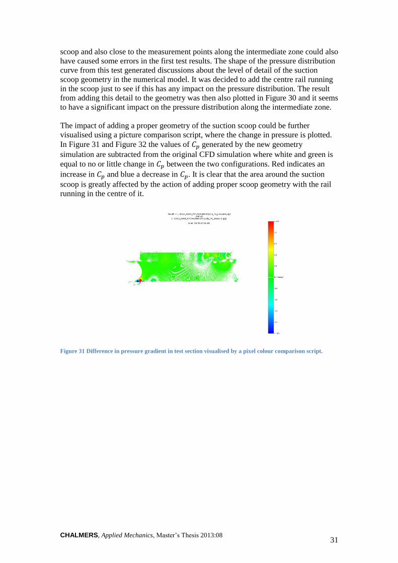
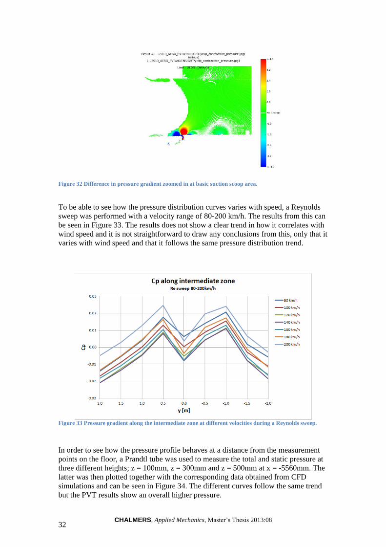
The impact of adding a proper geometry of the suction scoop could be further
visualised using a picture comparison script, where the change in pressure is plotted.
In Figure 31 and Figure 32 the values of generated by the new geometry
simulation are subtracted from the original CFD simulation where white and green is
equal to no or little change in between the two configurations. Red indicates an
increase in and blue a decrease in . It is clear that the area around the suction
scoop is greatly affected by the action of adding proper scoop geometry with the rail
running in the centre of it.
Figure 31 Difference in pressure gradient in test section visualised by a pixel colour comparison script.
CHALMERS, Applied Mechanics, Master’s Thesis 2013:08 32
Figure 32 Difference in pressure gradient zoomed in at basic suction scoop area.
To be able to see how the pressure distribution curves varies with speed, a Reynolds
sweep was performed with a velocity range of 80-200 km/h. The results from this can
be seen in Figure 33. The results does not show a clear trend in how it correlates with
wind speed and it is not straightforward to draw any conclusions from this, only that it
varies with wind speed and that it follows the same pressure distribution trend.
Figure 33 Pressure gradient along the intermediate zone at different velocities during a Reynolds sweep.
In order to see how the pressure profile behaves at a distance from the measurement
points on the floor, a Prandtl tube was used to measure the total and static pressure at
three different heights; z = 100mm, z = 300mm and z = 500mm at x = -5560mm. The
latter was then plotted together with the corresponding data obtained from CFD
simulations and can be seen in Figure 34. The different curves follow the same trend
but the PVT results show an overall higher pressure.
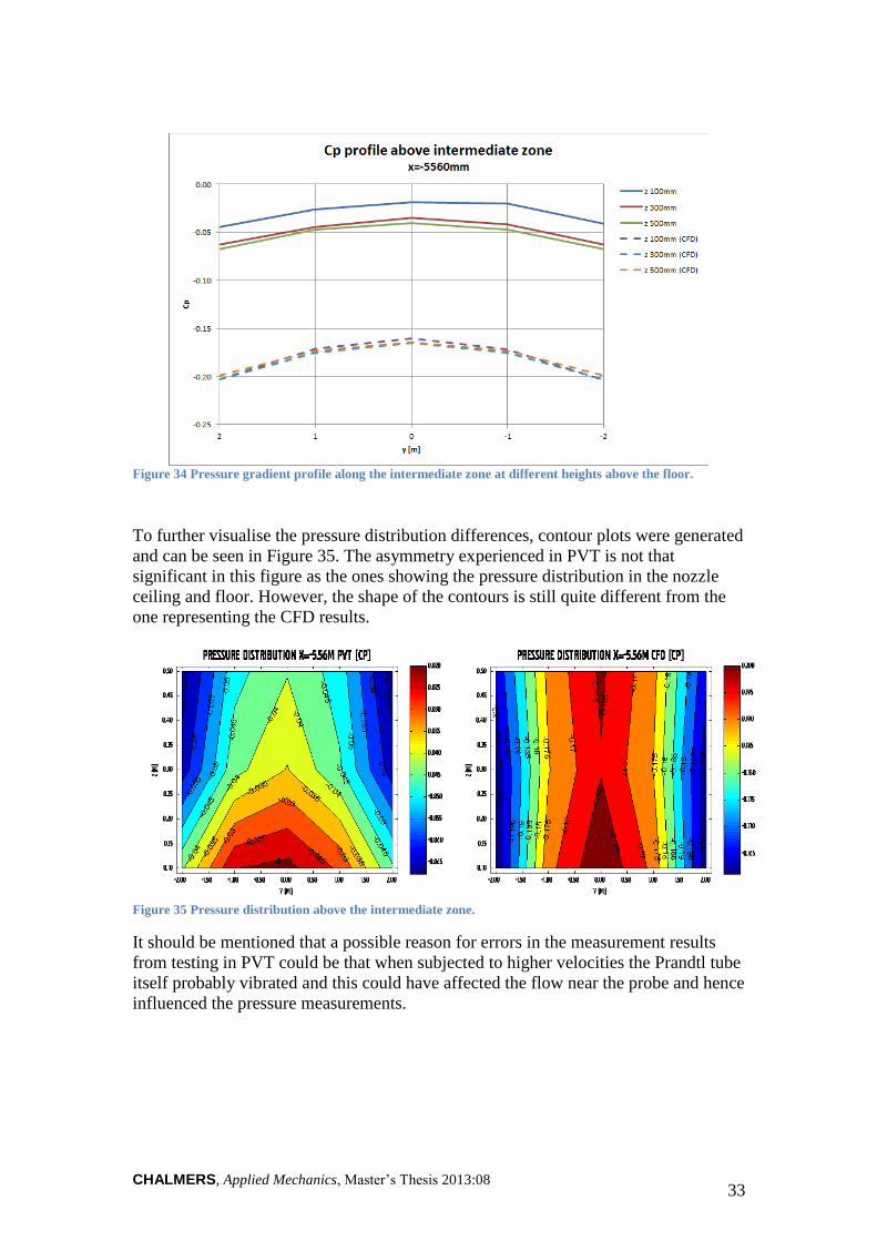
CHALMERS, Applied Mechanics, Master’s Thesis 2013:08 33
Figure 34 Pressure gradient profile along the intermediate zone at different heights above the floor.
To further visualise the pressure distribution differences, contour plots were generated
and can be seen in Figure 35. The asymmetry experienced in PVT is not that
significant in this figure as the ones showing the pressure distribution in the nozzle
ceiling and floor. However, the shape of the contours is still quite different from the
one representing the CFD results.
Figure 35 Pressure distribution above the intermediate zone.
It should be mentioned that a possible reason for errors in the measurement results
from testing in PVT could be that when subjected to higher velocities the Prandtl tube
itself probably vibrated and this could have affected the flow near the probe and hence
influenced the pressure measurements.

CHALMERS, Applied Mechanics, Master’s Thesis 2013:08 34
CHALMERS, Applied Mechanics, Master’s Thesis 2013:08 35
7 Discussion and conclusions
This part of the report outlines discussions about the results obtained during this thesis
and touching on possible sources of error. It finishes off with stating the conclusions
that can be drawn from the work performed and results obtained.
7.1 Discussion
The main focus of this thesis work has been to increase the understanding of the
complex flow field experienced in the VCC aerodynamic wind tunnel to be able to
model this in an accurate way with CFD.
Adding prism layer to the whole test section interior was a first attempt to try and
capture the major pressure drops experienced by the slotted walls on the right side of
the test section in PVT. The results show that the CFD tunnel is capturing these
pressure drops but the magnitude is still far from the PVT results. To further
investigate if the near wall flow is accurately resolved, it was decided to try to apply
the different wall functions available in ANSYS Fluent for the k-epsilon realisable
turbulence model. It was observed that the results from using standard wall function
and enhanced wall function were quite similar, indicating that the y+ values in the
tunnel are larger than 30 where the enhanced wall function applies the standard wall
function. Looking at the boundary layer profiles and also the pressure gradient along
the centreline it did however not have any significant impact on the results and it was
therefore decided to keep the default standard wall function used in the standard VCC
CFD procedure.
Apart from the non-uniformity observed at the left and right side slotted walls this
was also the case when post-processing the results from the two experimental tests in
PVT, partly focusing on the pressure distribution in the contraction ceiling and floor.
The question still remains why the CFD tunnel produces a more uniform flow field
than the PVT tunnel. The absence of the PVT tunnel’s closed air path which was left
out when the computational domain was restricted to the nozzle, test section and
diffuser cannot be neglected as a possible reason. Turning vanes and turbulence nets
are used in the PVT tunnel to create a uniform flow, but probably the flow still inhabit
some non-uniformity when it reaches the nozzle. Since the CFD inlet profile is set to a
uniform velocity inlet, this possible non-uniformity is not accounted for in the
simulations. Possible solutions for this will be further discussed in the Future work
chapter.
It is known that the empty PVT tunnel has a positive axial pressure gradient along the
test section centreline, meaning that the pressure is higher at the area where the
vehicle front usually is placed compared to where the rear and wake is situated.
Looking at the plots showing the pressure gradient along the centreline it is clear that
also the CFD tunnel experiences a positive axial pressure gradient but the pressure is
in general lower than what is measured in PVT. The difference is quite significant and
it is not straightforward to explain why. One thought that has been discussed is the
fact that is normalised in a different way than how it is usually done in order to
create a that is insensitive to atmospheric pressure and enable a correlation
between the reference pressures in the contraction and the ones measured at the centre
of the turntable (z=1200mm) used to define the free stream velocity at this point. This
normalisation equation and its calibration coefficients might have to be further
analysed to enable a more accurate match between the PVT and CFD results.
CHALMERS, Applied Mechanics, Master’s Thesis 2013:08 36
The action of adding proper suction scoop geometry to the numerical model generated
a significant difference in the pressure distribution profile along the intermediate
zone. It is interesting that at the floor the curve from the CFD simulations follows
the experimental results fairly well which it also does at some heights above these
measurements but with a greater offset in the magnitude of . Looking at the
boundary layer profiles created along the centrebelt with this additional scoop
geometry it did however not have any significant impact on these and further
investigation is needed. In PVT the leading edge of the centrebelt seem to create a
momentum deficit with a large velocity magnitude across a small height. This
propagates downstream the belt and the magnitude decreases with an increasing
height as the flow catches up. This boundary layer formation along the centrebelt is
not captured in the CFD simulations, and possible reasons could be the simplification
of the tunnel floor which is completely flat and there is no feature triggering this
velocity deficit. The impact of adding the suction scoop geometry does however stress
the importance of paying attention to details in the PVT geometry and make sure that
these are included in the model.
7.2 Conclusions
Based on the work performed, results obtained and objective stated in the Introduction
chapter of this thesis there are some main conclusions to be drawn.
An updated numerical model can be delivered to VCC, now containing a
detailed geometry of the basic suction scoop which clearly has proven to
contribute to the pressure distribution behaviour along the floor present PVT.
The CFD tunnel does however still not reproduce important flow parameters
like the pressure gradient along the centreline or the strong asymmetry in
pressure distribution in the nozzle ceiling and floor as they are measured in the
PVT tunnel. Therefore the CFD tunnel can still not be considered to accurately
simulate the flow field and more work needs to be done before it can be used
as an alternative to the standard computational domain used in the CFD
procedure at VCC today.
Adding boundary layers and employing the different wall functions available
in ANSYS Fluent did not enhance the capturing of the major pressure drops
experienced by the slotted walls on the right side of the test section.
To be able to get more information about how to simulate the flow field in the
test section, the inlet profile in the PVT tunnel needs to be measured and
reproduced in the CFD tunnel.
The flow in the PVT tunnel is a lot more asymmetric than what is showed by
the CFD tunnel results.
The geometry accuracy has proven to be an important factor when simulating
such a complex geometry as the PVT tunnel is. It is therefore important to gain
as much knowledge as possible about which details that do and do not have
significant impact on the flow field in PVT.
CHALMERS, Applied Mechanics, Master’s Thesis 2013:08 37
8 Recommendations for future work
To be able to reproduce the significant asymmetry in the flow field measured in PVT,
more knowledge about the inlet conditions needs to be obtained. In ANSYS Fluent it
is possible to define user defined inlet boundary conditions, so a recommendation
would be to in the future use the traverse gear available in PVT to measure the inlet
velocity/pressure profile at the test section entrance.
Another idea is naturally to consider adding a larger part of the closed air path to the
numerical model, preferably the first bend and turning vanes after the test section
which might have an impact on the axial pressure gradient in the CFD tunnel. In order
to do this, CAD models of these geometries needs to be generated and cleaned to be
used for simulations.
One thing that has been excluded from the scope of this study because of absence of
proper CAD data is the fact that there is a traversing unit mounted in the tunnel
ceiling which can be used for flow field pressure or velocity measurements. It is a
known fact that this traverse gear does affect the flow field in PVT. Work is currently
performed to generate an accurate CAD model of this traverse gear, and when this is
finalised a recommendation would be to insert this in to the CFD tunnel and run
simulations to obtain further information about how large impact this has on the flow
field.
An updated version of the software Harpoon used for volume meshing was in the
beginning of this thesis obtained to enable better management of prism layers and
avoiding cells collapsing at the end of PIDs. This version, 5.2beta5 is recommended
to use in the nearest future and it is also recommended to include the creation of the
prism layers in the configuration script since the model size hampers smooth working
in the GUI.
ANSYS Fluent 13.0.2 turned out to be the most stable solver to use in this thesis. It is
however recommended to try and use more recent releases to keep in line with the
versions used in the standard CFD procedure for Aerodynamic simulations at VCC.
One must thought pay attention to changes in the way operation questions are asked in
the new versions to be able to use the script created for this thesis in the future.
In this thesis the pressure gradient was normalised in the CFD tunnel the same way as
it is done in the PVT tunnel. However, based on the obtained results showing a
significant difference in axial pressure gradient between experiment and simulation it
is recommended to in the future further investigate how this is done and consider
alternative procedure for normalisation of .
As a final recommendation, further investigations on how to model the BLCS
accurately should be performed. In the existing model, the simplification of having a
completely flat floor could affect the boundary layer formation and propagation along
for example the centrebelt.

CHALMERS, Applied Mechanics, Master’s Thesis 2013:08 38
CHALMERS, Applied Mechanics, Master’s Thesis 2013:08 39
9 References
[1] (n.d.). Ansys Fluent User's Guide. Release 12.0, 2009-01-29.
[2] Barnard, R. H. (2009). Road Vehicle Aerodynamic Design - An introduction.
St Albands, Hertfordshire: MechAero Publishing.
[3] Bender, T. J. (2006). Commissioning Report: PVT Ground Simulation
Upgrade. Aiolos Report Number: 4147R269: Volvo Car Corporation and
Aiolos Engineering Corporation.
[4] Cederlund, J., & Vikström, J. (2010). The Aerodynamic Influence of Rim
Design on a Sports Car and its Interaction with the Wing and Diffuser Flow.
Göteborg: Department of Applied Mechanics, Chalmers University of
Technology.
[5] Cyr, S., Ih, K.-D., & Park, S.-H. (2011). Accurate Reproduction of Wind-
Tunnel Results with CFD. SAE Technical Paper 2011-01-0158, 2011, doi
10.4271/2011-01-0158.
[6] Davidsson, L. (2011). An Introduction to Turbulence Models. Göteborg:
Department of Thermo and Fluid Dynamics: Chalmers University of
Technology.
[7] El Gharbi, N.; Absi, R.; Benzaoui, A.; Amara, E.H. (2009). Effect of near-wal
treatments on airflow simulations. International Conference on Computational
Methods for Energy Engineering and Environment, (pp. 185-189). Sousse,
Tunisia.
[8] Eng, M. (2009). Investigation of Aerodynamic correction methods applied to a
slotted wall wind tunnel. Master thesis performed at Volvo Cars, Technishe
Universität Berlin.
[9] LEAP Support Team, LEAP Australia Py Ltd. (2012, June 25). Tips & Tricks:
Turbulence Part 2 – Wall Functions and Y+ requirements. Australia.
[10] Olander, M. (2011). CFD Simulation of the Volvo Cars Slotted Walls Wind
Tunnel. Göteborg: Master Thesis performed at Volvo Cars, Chalmers
University of Technology.
[11] Pitman, J. (2012). Recent Experience in Aerodynamics Simulation ECARA
Sub-group: CFD. Heritage Motor Centre. Jaguar Land-Rover.
[12] Sternéus, J; Walker, T; Bender, T. (2007). Upgrade of the Volvo Cars
Aerodynamic Wind Tunnel. SAE Technical Paper 2007-01-1043.
[13] Versteeg, H., & Malalasekera, W. (2007). An Introduction to Computational
Fluid Dynamics, The Finite Volume Method. 2nd edition, Pearson Education
Limited.
[14] White, F. M. (2008). Fluid Mechanics. McGraw-Hilll Higher Education.
[15] LLC., F. K. (2002, November 12). Flowmeter Directory. Retrieved July 3,
2013, from USING A PITOT STATIC TUBE FOR VELOCITY AND FLOW
RATE MEASUREMENT:
http://www.flowmeterdirectory.com/flowmeter_artc_02111201.html

CHALMERS, Applied Mechanics, Master’s Thesis 2013:08 40
CHALMERS, Applied Mechanics, Master’s Thesis 2013:08 I
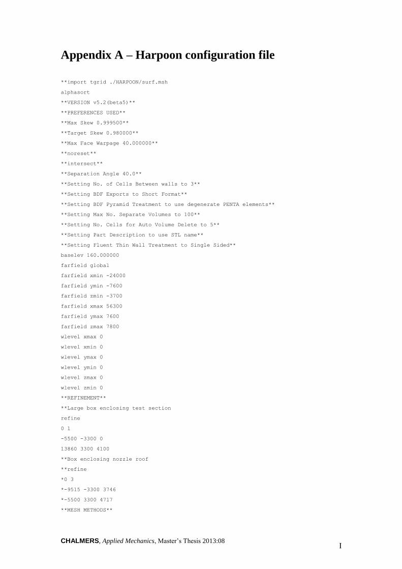
Appendix A – Harpoon configuration file
**import tgrid ./HARPOON/surf.msh
alphasort
**VERSION v5.2(beta5)**
**PREFERENCES USED**
**Max Skew 0.999500**
**Target Skew 0.980000**
**Max Face Warpage 40.000000**
**noreset**
**intersect**
**Separation Angle 40.0**
**Setting No. of Cells Between walls to 3**
**Setting BDF Exports to Short Format**
**Setting BDF Pyramid Treatment to use degenerate PENTA elements**
**Setting Max No. Separate Volumes to 100**
**Setting No. Cells for Auto Volume Delete to 5**
**Setting Part Description to use STL name**
**Setting Fluent Thin Wall Treatment to Single Sided**
baselev 160.000000
farfield global
farfield xmin -24000
farfield ymin -7600
farfield zmin -3700
farfield xmax 56300
farfield ymax 7600
farfield zmax 7800
wlevel xmax 0
wlevel xmin 0
wlevel ymax 0
wlevel ymin 0
wlevel zmax 0
wlevel zmin 0
**REFINEMENT**
**Large box enclosing test section
refine
0 1
-5500 -3300 0
13860 3300 4100
**Box enclosing nozzle roof
**refine
*0 3
*-9515 -3300 3746
*-5500 3300 4717
**MESH METHODS**
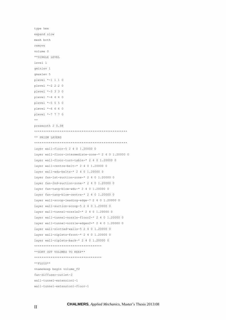
CHALMERS, Applied Mechanics, Master’s Thesis 2013:08 II
type hex
expand slow
mesh both
remove
volume 0
**SINGLE LEVEL
level 1
gminlev 1
gmaxlev 5
plevel *-1 1 1 0
plevel *-2 2 2 0
plevel *-3 3 3 0
plevel *-4 4 4 0
plevel *-5 5 5 0
plevel *-6 6 6 0
plevel *-7 7 7 0
**
presmooth 2 0.98
***************************************************
** PRISM LAYERS
***************************************************
layer wall-floor-5 2 4 0 1.20000 0
layer wall-floor-intermediate-zone-* 2 4 0 1.20000 0
layer wall-floor-turn-table-* 2 4 0 1.20000 0
layer wall-centre-belt-* 2 4 0 1.20000 0
layer wall-wdu-belts-* 2 4 0 1.20000 0
layer fan-1st-suction-zone-* 2 4 0 1.20000 0
layer fan-2nd-suction-zone-* 2 4 0 1.20000 0
layer fan-tang-blow-wdu-* 2 4 0 1.20000 0
layer fan-tang-blow-centre-* 2 4 0 1.20000 0
layer wall-scoop-leading-edge-7 2 4 0 1.20000 0
layer wall-suction-scoop-5 2 4 0 1.20000 0
layer wall-tunnel-nozzle2-* 2 4 0 1.20000 0
layer wall-tunnel-nozzle-floor2-* 2 4 0 1.20000 0
layer wall-tunnel-nozzle-edges2-* 2 4 0 1.20000 0
layer wall-slotted-walls-5 2 4 0 1.20000 0
layer wall-riplets-front-* 2 4 0 1.20000 0
layer wall-riplets-back-* 2 4 0 1.20000 0
*************************************
**SORT OUT VOLUMES TO KEEP**
*************************************
**FLUID**
vnamekeep begin volume_f2
fan-diffuser-outlet-2
wall-tunnel-extension1-1
wall-tunnel-extension1-floor-1
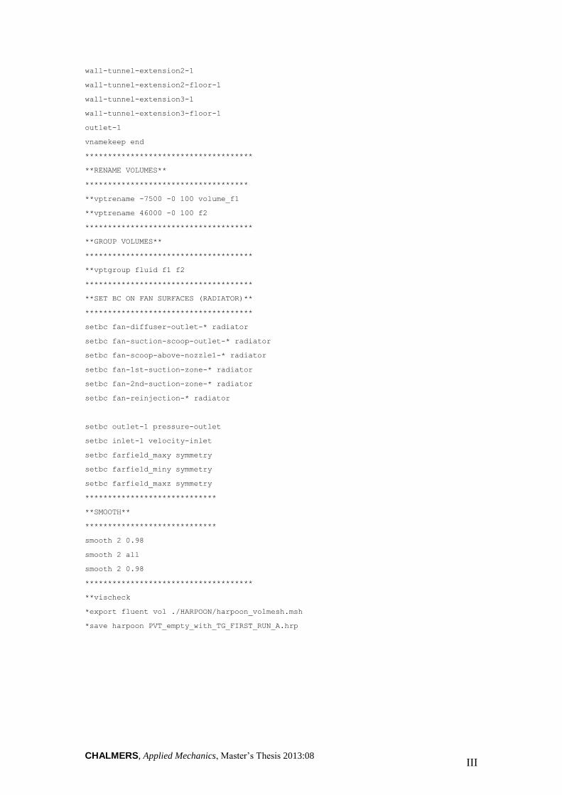
CHALMERS, Applied Mechanics, Master’s Thesis 2013:08 III
wall-tunnel-extension2-1
wall-tunnel-extension2-floor-1
wall-tunnel-extension3-1
wall-tunnel-extension3-floor-1
outlet-1
vnamekeep end
*************************************
**RENAME VOLUMES**
************************************
**vptrename -7500 -0 100 volume_f1
**vptrename 46000 -0 100 f2
*************************************
**GROUP VOLUMES**
*************************************
**vptgroup fluid f1 f2
*************************************
**SET BC ON FAN SURFACES (RADIATOR)**
*************************************
setbc fan-diffuser-outlet-* radiator
setbc fan-suction-scoop-outlet-* radiator
setbc fan-scoop-above-nozzle1-* radiator
setbc fan-1st-suction-zone-* radiator
setbc fan-2nd-suction-zone-* radiator
setbc fan-reinjection-* radiator
setbc outlet-1 pressure-outlet
setbc inlet-1 velocity-inlet
setbc farfield_maxy symmetry
setbc farfield_miny symmetry
setbc farfield_maxz symmetry
*****************************
**SMOOTH**
*****************************
smooth 2 0.98
smooth 2 all
smooth 2 0.98
*************************************
**vischeck
*export fluent vol ./HARPOON/harpoon_volmesh.msh
*save harpoon PVT_empty_with_TG_FIRST_RUN_A.hrp

CHALMERS, Applied Mechanics, Master’s Thesis 2013:08 IV
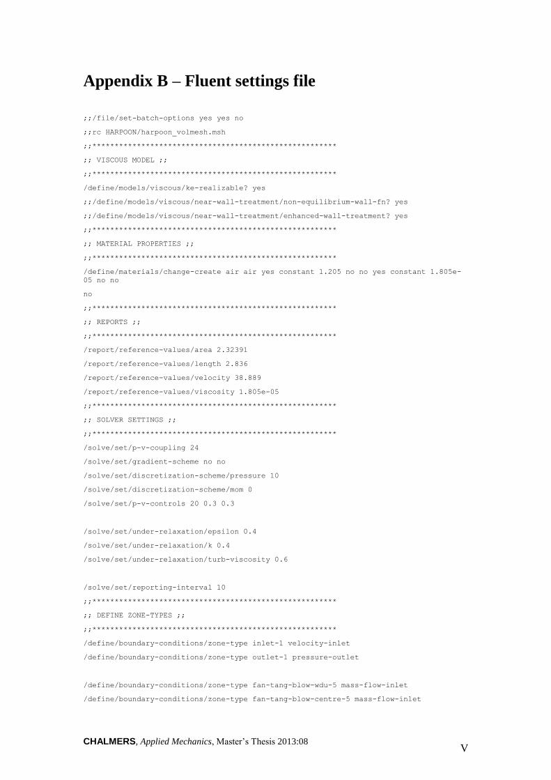
CHALMERS, Applied Mechanics, Master’s Thesis 2013:08 V
Appendix B – Fluent settings file
;;/file/set-batch-options yes yes no
;;rc HARPOON/harpoon_volmesh.msh
;;*******************************************************
;; VISCOUS MODEL ;;
;;*******************************************************
/define/models/viscous/ke-realizable? yes
;;/define/models/viscous/near-wall-treatment/non-equilibrium-wall-fn? yes
;;/define/models/viscous/near-wall-treatment/enhanced-wall-treatment? yes
;;*******************************************************
;; MATERIAL PROPERTIES ;;
;;*******************************************************
/define/materials/change-create air air yes constant 1.205 no no yes constant 1.805e-
05 no no
no
;;*******************************************************
;; REPORTS ;;
;;*******************************************************
/report/reference-values/area 2.32391
/report/reference-values/length 2.836
/report/reference-values/velocity 38.889
/report/reference-values/viscosity 1.805e-05
;;*******************************************************
;; SOLVER SETTINGS ;;
;;*******************************************************
/solve/set/p-v-coupling 24
/solve/set/gradient-scheme no no
/solve/set/discretization-scheme/pressure 10
/solve/set/discretization-scheme/mom 0
/solve/set/p-v-controls 20 0.3 0.3
/solve/set/under-relaxation/epsilon 0.4
/solve/set/under-relaxation/k 0.4
/solve/set/under-relaxation/turb-viscosity 0.6
/solve/set/reporting-interval 10
;;*******************************************************
;; DEFINE ZONE-TYPES ;;
;;*******************************************************
/define/boundary-conditions/zone-type inlet-1 velocity-inlet
/define/boundary-conditions/zone-type outlet-1 pressure-outlet
/define/boundary-conditions/zone-type fan-tang-blow-wdu-5 mass-flow-inlet
/define/boundary-conditions/zone-type fan-tang-blow-centre-5 mass-flow-inlet
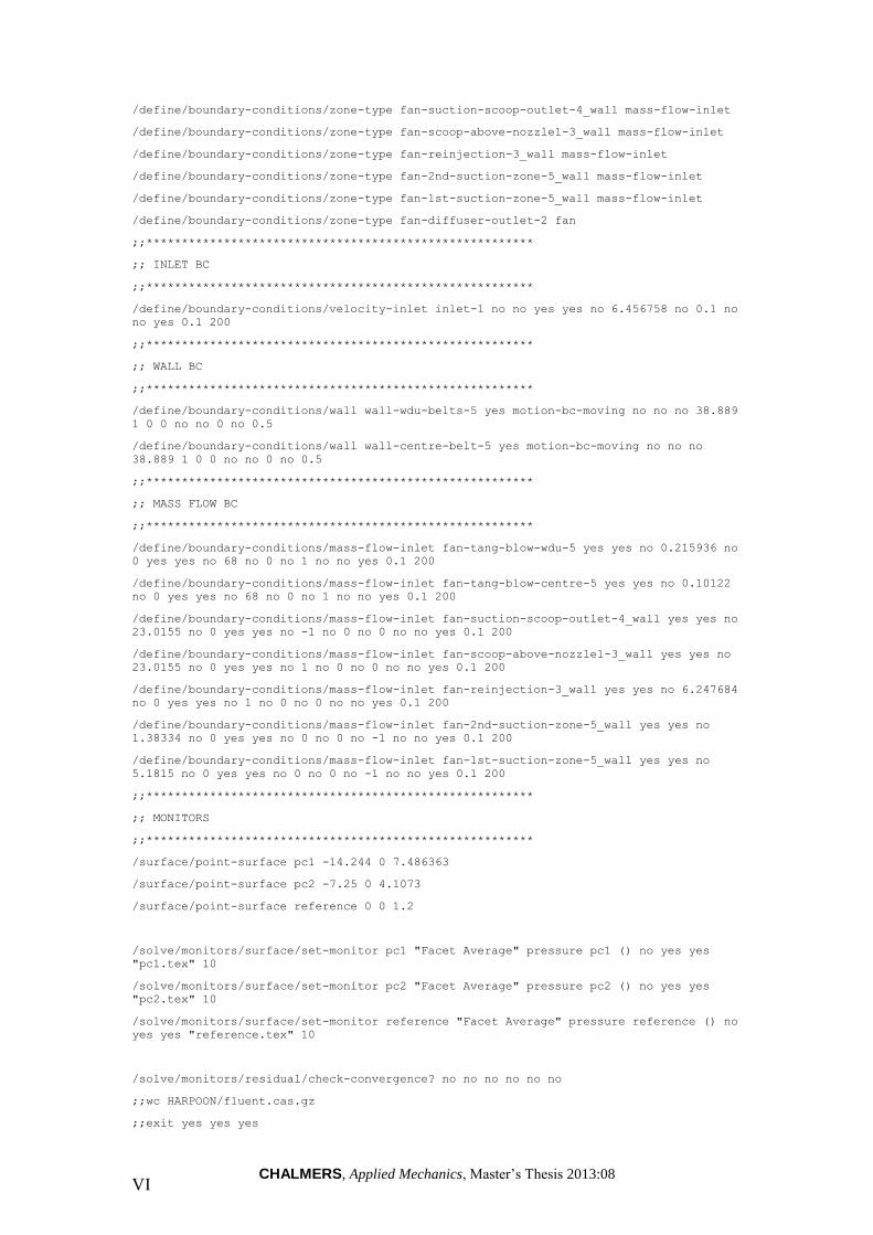
CHALMERS, Applied Mechanics, Master’s Thesis 2013:08 VI
/define/boundary-conditions/zone-type fan-suction-scoop-outlet-4_wall mass-flow-inlet
/define/boundary-conditions/zone-type fan-scoop-above-nozzle1-3_wall mass-flow-inlet
/define/boundary-conditions/zone-type fan-reinjection-3_wall mass-flow-inlet
/define/boundary-conditions/zone-type fan-2nd-suction-zone-5_wall mass-flow-inlet
/define/boundary-conditions/zone-type fan-1st-suction-zone-5_wall mass-flow-inlet
/define/boundary-conditions/zone-type fan-diffuser-outlet-2 fan
;;*******************************************************
;; INLET BC
;;*******************************************************
/define/boundary-conditions/velocity-inlet inlet-1 no no yes yes no 6.456758 no 0.1 no
no yes 0.1 200
;;*******************************************************
;; WALL BC
;;*******************************************************
/define/boundary-conditions/wall wall-wdu-belts-5 yes motion-bc-moving no no no 38.889
1 0 0 no no 0 no 0.5
/define/boundary-conditions/wall wall-centre-belt-5 yes motion-bc-moving no no no
38.889 1 0 0 no no 0 no 0.5
;;*******************************************************
;; MASS FLOW BC
;;*******************************************************
/define/boundary-conditions/mass-flow-inlet fan-tang-blow-wdu-5 yes yes no 0.215936 no
0 yes yes no 68 no 0 no 1 no no yes 0.1 200
/define/boundary-conditions/mass-flow-inlet fan-tang-blow-centre-5 yes yes no 0.10122
no 0 yes yes no 68 no 0 no 1 no no yes 0.1 200
/define/boundary-conditions/mass-flow-inlet fan-suction-scoop-outlet-4_wall yes yes no
23.0155 no 0 yes yes no -1 no 0 no 0 no no yes 0.1 200
/define/boundary-conditions/mass-flow-inlet fan-scoop-above-nozzle1-3_wall yes yes no
23.0155 no 0 yes yes no 1 no 0 no 0 no no yes 0.1 200
/define/boundary-conditions/mass-flow-inlet fan-reinjection-3_wall yes yes no 6.247684
no 0 yes yes no 1 no 0 no 0 no no yes 0.1 200
/define/boundary-conditions/mass-flow-inlet fan-2nd-suction-zone-5_wall yes yes no
1.38334 no 0 yes yes no 0 no 0 no -1 no no yes 0.1 200
/define/boundary-conditions/mass-flow-inlet fan-1st-suction-zone-5_wall yes yes no
5.1815 no 0 yes yes no 0 no 0 no -1 no no yes 0.1 200
;;*******************************************************
;; MONITORS
;;*******************************************************
/surface/point-surface pc1 -14.244 0 7.486363
/surface/point-surface pc2 -7.25 0 4.1073
/surface/point-surface reference 0 0 1.2
/solve/monitors/surface/set-monitor pc1 "Facet Average" pressure pc1 () no yes yes
"pc1.tex" 10
/solve/monitors/surface/set-monitor pc2 "Facet Average" pressure pc2 () no yes yes
"pc2.tex" 10
/solve/monitors/surface/set-monitor reference "Facet Average" pressure reference () no
yes yes "reference.tex" 10
/solve/monitors/residual/check-convergence? no no no no no no
;;wc HARPOON/fluent.cas.gz
;;exit yes yes yes

CHALMERS, Applied Mechanics, Master’s Thesis 2013:08 VII
Appendix C – Fluent run file
/file/set-batch-options yes yes no
rc HARPOON/fluent.cas.gz
/grid/scale
0.001
0.001
0.001
;;;;;;;;;;;;;;;;;;;;;;;;;;;;;;;;;;;;;;;;;;;;;;;;;;;;;;;;;
;; Check mesh quality/Smooth mesh
;;;;;;;;;;;;;;;;;;;;;;;;;;;;;;;;;;;;;;;;;;;;;;;;;;;;;;;;;
/mesh/quality
/mesh/smooth-mesh
"quality based"
4
0.0005
/mesh/quality
;;;;;;;;;;;;;;;;;;;;;;;;;;;;;;;;;;;;;;;;;;;;;;;;;;;;;;;;;
;; Initialize
;;;;;;;;;;;;;;;;;;;;;;;;;;;;;;;;;;;;;;;;;;;;;;;;;;;;;;;;;
/solve/initialize/initialize-flow
/solve/initialize/fmg-initialization/
yes
;;
;;
;;;;;;;;;;;;;;;;;;;;;;;;;;;;;;;;;;;;;;;;;;;;;;;;;;;;;;;;;
;; First order scheme
;;;;;;;;;;;;;;;;;;;;;;;;;;;;;;;;;;;;;;;;;;;;;;;;;;;;;;;;;
solve/iterate 500
wcd FLUENT/fluent-it500.cas.gz
;;
;;;;;;;;;;;;;;;;;;;;;;;;;;;;;;;;;;;;;;;;;;;;;;;;;;;;;;;;;
;; Second order scheme
;;;;;;;;;;;;;;;;;;;;;;;;;;;;;;;;;;;;;;;;;;;;;;;;;;;;;;;;;
/solve/set/discretization-scheme/mom
1
q
q
q
q
;;;;;;;;;;;;;;;;;;;;;;;;;;;;;;;;;;;;;;;;;;;;;;;;;;;;;;;;;
;; iteration_start
;;;;;;;;;;;;;;;;;;;;;;;;;;;;;;;;;;;;;;;;;;;;;;;;;;;;;;;;;
solve/iterate 2000
;;
wcd FLUENT/fluent-it2500.cas.gz
CHALMERS, Applied Mechanics, Master’s Thesis 2013:08 VIII
;;
;; ***************Report forces**************
;;
/report/forces/wall-forces
y
1
0
0
n
;;
;;
;;**************Report fluxes***************
;;
/report/fluxes/mass-flow
n
outlet-*
,
n
;;
;;**************Export Ensight Files in nobackup***************
;;
/file/export/ensight-gold
ENSIGHT/ensight
pressure
total-pressure
skin-friction-coef
x-wall-shear
z-wall-shear
x-face-area
y-face-area
z-face-area
y-plus
q
yes
()
no
/file/export/ensight-gold
ENSIGHT/ensight_cell
pressure
total-pressure
skin-friction-coef
x-wall-shear
z-wall-shear
x-face-area
y-face-area
z-face-area

CHALMERS, Applied Mechanics, Master’s Thesis 2013:08 IX
y-plus
q
yes
()
yes
;;
exit yes yes yes

CHALMERS, Applied Mechanics, Master’s Thesis 2013:08 X
CHALMERS, Applied Mechanics, Master’s Thesis 2013:08 XI
Appendix D – EnSight post processing file #########################################################
##
## ENSIGHT PYTHON SCRIPT
##
#########################################################
#########################################################
##
## CREATING GROUPS AND VARIABLES
##
#########################################################
ensight.part.select_byexpr_begin("(CASE:Case 1)*fan-slott-right*")
ensight.part.group("fan-slott-right")
ensight.part.select_byexpr_begin("(CASE:Case 1)*fan-slott-left*")
ensight.part.group("fan-slott-left")
ensight.part.select_byexpr_begin("(CASE:Case 1)*fan-slott-top*")
ensight.part.group("fan-slott-top")
ensight.part.select_byexpr_begin("(CASE:Case1)*wall-floor*","(CASE:Case 1)*wall-
centre-belt*","(CASE:Case 1)*wall-wdu-belts*")
ensight.part.group("wall-floor")
ensight.part.select_byexpr_begin("(CASE:Case1)*fan-
tang*","(CASE:Case1)*zone*","(CASE:Case 1)*fan-reinjection*","(CASE:Case 1)*scoop*")
ensight.part.group("fan-BLCS")
ensight.part.select_byexpr_begin("(CASE:Case 1)*wall-riplets-back*")
ensight.part.group("wall-riplets-back")
ensight.part.select_byexpr_begin("(CASE:Case 1)*wall-riplets-front*","(CASE:Case
1)*baffle-riplets-front*")
ensight.part.group("wall-riplets-front")
ensight.part.select_byexpr_begin("(CASE:Case 1)*wall-roof-flap*")
ensight.part.group("wall-roof-flap")
ensight.part.select_byexpr_begin("(CASE:Case 1)*wall-side-flap1*")
ensight.part.group("wall-side-flap1")
ensight.part.select_byexpr_begin("(CASE:Case 1)*wall-side-flap2*")
ensight.part.group("wall-side-flap2")
ensight.part.select_byexpr_begin("(CASE:Case 1)*wall-slotted-walls*","(CASE:Case
1)*baffle-slotted-walls*","(CASE:Case 1)*wall-ventilation*","(CASE:Case 1)*wall-
inner*")
ensight.part.group("wall-slotted-walls")
ensight.part.select_byexpr_begin("(CASE:Case 1)*wall-tunnel-diffuser*","(CASE:Case
1)*fan-diffuser-outlet*")
ensight.part.group("wall-tunnel-diffuser")
ensight.part.select_byexpr_begin("(CASE:Case 1)*wall-tunnel-entrance*")
ensight.part.group("wall-tunnel-entrance")
ensight.part.select_byexpr_begin("(CASE:Case 1)*wall-tunnel-extension*")
ensight.part.group("wall-tunnel-extension")
ensight.part.select_byexpr_begin("(CASE:Case 1)*wall-tunnel-nozzle*")
ensight.part.group("wall-tunnel-nozzle")
ensight.part.select_byexpr_begin("(CASE:Case 1)*wall-tg*")
CHALMERS, Applied Mechanics, Master’s Thesis 2013:08 XII
ensight.part.group("wall-TG")
ensight.part.select_byexpr_begin("(CASE:Case 1)*wall-tunnel-test*")
ensight.part.group("wall-tunnel-test")
ensight.part.select_byexpr_begin("(CASE:Case 1)*fluid*","(CASE:Case 1)*volume*")
ensight.part.group("fluid")
#########################################################
##
## CREATING VARIABLES
##
#########################################################
ensight.part.select_all()
ensight.variables.activate_all()
ensight.variables.evaluate("ref_stat_pres = -325.497")
ensight.variables.evaluate("ref_dyn_pres = 0.5*1.205*38.889^2")
ensight.variables.evaluate("Pc1 = 559.373")
ensight.variables.evaluate("Pc2 = -334.834")
ensight.variables.evaluate("dp = Pc1-Pc2")
ensight.variables.evaluate("kq = ref_dyn_pres/dp")
ensight.variables.evaluate("kp = (ref_stat_pres-Pc2)/dp")
ensight.variables.evaluate("Cp_64 = (pressure-Pc2)/(dp*kq)-kp/kq")
ensight.variables.evaluate("cp = pressure/ref_dyn_pres")
ensight.variables.evaluate("cp_tot = total_pressure/ref_dyn_pres")
ensight.variables.evaluate("x_vel = velocity[x]")
ensight.variables.evaluate("y_vel = velocity[y]")
ensight.variables.evaluate("z_vel = velocity[z]")
#########################################################
##
## QUERY AND EXPORT CP ALONG CENTRELINE VALUES
##
#########################################################
ensight.sendmesgoptions(version="9.22a")
ensight.part.select_byname_begin("(CASE:Case 1)GROUP: fluid")
ensight.query_ent_var.begin()
ensight.query_ent_var.description("")
ensight.query_ent_var.query_type("generated")
ensight.query_ent_var.number_of_sample_pts(200)
ensight.query_ent_var.constrain("line_tool")
ensight.query_ent_var.line_loc(1,-4.000000,0.000000,0.100000)
ensight.query_ent_var.line_loc(2,10.000000,0.000000,0.100000)
ensight.query_ent_var.distance("x_from_origin")
ensight.query_ent_var.variable_1("Cp_64")
ensight.query_ent_var.generate_over("distance")
ensight.query_ent_var.variable_2("DISTANCE")
ensight.query_ent_var.end()
ensight.query_ent_var.query()
ensight.curve.select_begin(0)
CHALMERS, Applied Mechanics, Master’s Thesis 2013:08 XIII
ensight.view_transf.function("line")
ensight.view_transf.line(1,-4.000000e+000,0.000000e+000,3.000000e-001)
ensight.view_transf.line(2,1.000000e+001,0.000000e+000,3.000000e-001)
ensight.query_ent_var.begin()
ensight.query_ent_var.description("")
ensight.query_ent_var.query_type("generated")
ensight.query_ent_var.number_of_sample_pts(200)
ensight.query_ent_var.constrain("line_tool")
ensight.query_ent_var.line_loc(1,-4.000000,0.000000,0.300000)
ensight.query_ent_var.line_loc(2,10.000000,0.000000,0.300000)
ensight.query_ent_var.distance("x_from_origin")
ensight.query_ent_var.variable_1("Cp_64")
ensight.query_ent_var.generate_over("distance")
ensight.query_ent_var.variable_2("DISTANCE")
ensight.query_ent_var.end()
ensight.query_ent_var.query()
ensight.curve.select_begin(1)
ensight.view_transf.function("line")
ensight.view_transf.line(1,-4.000000e+000,0.000000e+000,6.000000e-001)
ensight.view_transf.line(2,1.000000e+001,0.000000e+000,6.000000e-001)
ensight.query_ent_var.begin()
ensight.query_ent_var.description("")
ensight.query_ent_var.query_type("generated")
ensight.query_ent_var.number_of_sample_pts(200)
ensight.query_ent_var.constrain("line_tool")
ensight.query_ent_var.line_loc(1,-4.000000,0.000000,0.600000)
ensight.query_ent_var.line_loc(2,10.000000,0.000000,0.600000)
ensight.query_ent_var.distance("x_from_origin")
ensight.query_ent_var.variable_1("Cp_64")
ensight.query_ent_var.generate_over("distance")
ensight.query_ent_var.variable_2("DISTANCE")
ensight.query_ent_var.end()
ensight.query_ent_var.query()
ensight.curve.select_begin(2)
ensight.view_transf.function("line")
ensight.view_transf.line(1,-4.000000e+000,0.000000e+000,9.000000e-001)
ensight.view_transf.line(2,1.000000e+001,0.000000e+000,9.000000e-001)
ensight.query_ent_var.begin()
ensight.query_ent_var.description("")
ensight.query_ent_var.query_type("generated")
ensight.query_ent_var.number_of_sample_pts(200)
ensight.query_ent_var.constrain("line_tool")
ensight.query_ent_var.line_loc(1,-4.000000,0.000000,0.900000)
ensight.query_ent_var.line_loc(2,10.000000,0.000000,0.900000)
ensight.query_ent_var.distance("x_from_origin")
ensight.query_ent_var.variable_1("Cp_64")
CHALMERS, Applied Mechanics, Master’s Thesis 2013:08 XIV
ensight.query_ent_var.generate_over("distance")
ensight.query_ent_var.variable_2("DISTANCE")
ensight.query_ent_var.end()
ensight.query_ent_var.query()
ensight.curve.select_begin(3)
ensight.curve.select_begin(0)
ensight.view_transf.function("global")
ensight.curve.desc("z100mm")
ensight.curve.select_begin(1)
ensight.curve.desc("z300mm")
ensight.curve.select_begin(2)
ensight.curve.desc("z600mm")
ensight.curve.select_begin(3)
ensight.curve.desc("z900mm")
ensight.curve.select_begin(0)
ensight.view_transf.function("global")
ensight.curve.assign("rescale","z100mm")
ensight.plot.select_begin(0)
ensight.plot.select_default()
ensight.curve.select_begin(1)
ensight.plot.select_begin(0)
ensight.curve.assign("rescale")
ensight.plot.select_default()
ensight.curve.select_begin(2)
ensight.plot.select_begin(0)
ensight.curve.assign("rescale")
ensight.plot.select_default()
ensight.curve.select_begin(3)
ensight.plot.select_begin(0)
ensight.curve.assign("rescale")
ensight.view_transf.function("global")
ensight.plot.plot_title("Cp at centreline")
ensight.view_transf.function("global")
ensight.curve.select_begin(0)
ensight.curve.save("xy_data","xy_cp_centreline_z100mm")
ensight.curve.select_begin(1)
ensight.curve.save("xy_data","xy_cp_centreline_z300mm")
ensight.curve.select_begin(2)
ensight.curve.save("xy_data","xy_cp_centreline_z600mm")
ensight.curve.select_begin(3)
ensight.curve.save("xy_data","xy_cp_centreline_z900mm")
#########################################################
##
## QUERY AND EXPORT CP AT WALL ALONG 2ND SLOT VALUES
##
#########################################################
CHALMERS, Applied Mechanics, Master’s Thesis 2013:08 XV
ensight.sendmesgoptions(version="9.22a")
ensight.part.select_byname_begin("(CASE:Case 1)GROUP: fluid")
ensight.query_ent_var.begin()
ensight.query_ent_var.description("")
ensight.query_ent_var.query_type("generated")
ensight.query_ent_var.number_of_sample_pts(200)
ensight.query_ent_var.constrain("line_tool")
ensight.query_ent_var.line_loc(1,-4.000000,3.300000,0.707500)
ensight.query_ent_var.line_loc(2,10.000000,3.300000,0.707500)
ensight.query_ent_var.distance("x_from_origin")
ensight.query_ent_var.variable_1("Cp_64")
ensight.query_ent_var.generate_over("distance")
ensight.query_ent_var.variable_2("DISTANCE")
ensight.query_ent_var.end()
ensight.query_ent_var.query()
ensight.curve.select_begin(0)
ensight.curve.desc("Right side")
ensight.curve.rgb(1.000000e+000,0.000000e+000,0.000000e+000)
ensight.query_ent_var.begin()
ensight.query_ent_var.description("")
ensight.query_ent_var.query_type("generated")
ensight.query_ent_var.number_of_sample_pts(200)
ensight.query_ent_var.constrain("line_tool")
ensight.query_ent_var.line_loc(1,-4.000000,-3.300000,0.707500)
ensight.query_ent_var.line_loc(2,10.000000,-3.300000,0.707500)
ensight.query_ent_var.distance("x_from_origin")
ensight.query_ent_var.variable_1("Cp_64")
ensight.query_ent_var.generate_over("distance")
ensight.query_ent_var.variable_2("DISTANCE")
ensight.query_ent_var.end()
ensight.query_ent_var.query()
ensight.curve.select_begin(1)
ensight.curve.desc("Left side")
ensight.curve.assign("rescale","Cp","at","wall","z=0.7075m")
ensight.curve.rgb(0.000000e+000,0.000000e+000,1.000000e+000)
ensight.curve.marker("circle")
ensight.plot.select_begin(0)
ensight.plot.origin_x(0.000000e+000)
ensight.plot.origin_y(0.000000e+000)
ensight.plot.width(1.000000e+000)
ensight.plot.height(1.000000e+000)
ensight.plot.legend_origin_x(8.000000e-001)
ensight.plot.legend_origin_y(9.500000e-001)
ensight.plot.legend_textsize(2.000000e+001)
ensight.plot.axis_x_title("x")
ensight.curve.select_begin(0)

CHALMERS, Applied Mechanics, Master’s Thesis 2013:08 XVI
ensight.plot.select_begin(0)
ensight.curve.assign("rescale")
ensight.sendmesgoptions(version=0)
ensight.curve.select_begin(0)
ensight.curve.save("xy_data","xy_cp64_at_wall_z07075m_RS")
ensight.curve.select_begin(1)
ensight.curve.save("xy_data","xy_cp64_at_wall_z07075m_LS")