Simulated Annealing

G.Anuradha

What is it?

• Simulated Annealing is a stochastic optimization method that derives its name from the annealing process used to re-crystallize metals

• Comes under the category of evolutionary techniques of optimization

What is annealing?

• Annealing is a heat process whereby a metal is heated to a specific temperature and then allowed to cool slowly. This softens the metal which means it can be cut and shaped more easily

What happens during annealing?

• Initially when the metal is heated to high temperatures, the atoms have lots of space to move about

• Slowly when the temperature is reduced the movement of free atoms are slowly reduced and finally the metals crystallize themselves

Relation between annealing and simulated annealing

• Simulated annealing is analogous to this annealing process.

• Initially the search area is more, there input parameters are searched in more random space and slow with each iteration this space reduces.

• This helps in achieving global optimized value, although it takes much more time for optimizing

Analogy between annealing and simulated annealing

• Annealing– Energy in thermodynamic

system– high-mobility atoms are

trying to orient themselves with other nonlocal atoms and the energy state can occasionally go up.

– low-mobility atoms can only orient themselves with local atoms and the energy state is not likely to go up again.

• Simulated Annealing– Value of objective function– At high temperatures, SA

allows fn. evaluations at faraway points and it is likely to accept a new point.

– At low temperatures, SA evaluates the objective function only at local points and the likelihood of it accepting a new point with higher energy is much lower.

Cooling Schedule

• how rapidly the temperature is lowered from high to low values.

• This is usually application specific and requires some experimentation by trial-and-error.

Fundamental terminologies in SA

• Objective function • Generating function • Acceptance function • Annealing schedule

Objective function

• E = f(x), where each x is viewed as a point in an input space.

• The task of SA is to sample the input space effectively to find an x that minimizes E.

Generating function

• A generating function specifies the probability density function of the difference between the current point and the next point to be visited.

• is a random variable with probability density function g(∆x, T), where T is the temperature.

Acceptance function

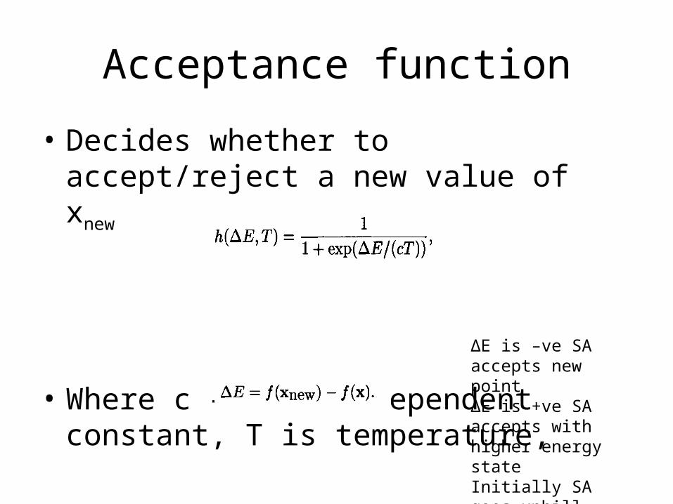
• Decides whether to accept/reject a new value of xnew

• Where c – system dependent constant, T is temperature,

∆E is –ve SA accepts new point∆E is +ve SA accepts with higher energy stateInitially SA goes uphill and downhill

Annealing schedule

• decrease the temperature T by a certain percentage at each iteration.

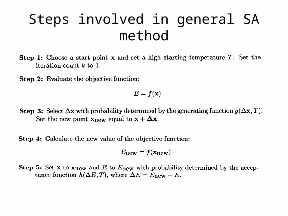
Steps involved in general SA method

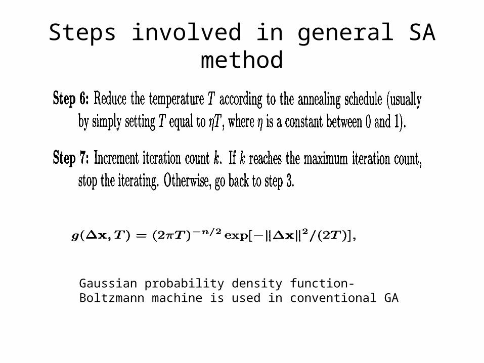
Steps involved in general SA method

Gaussian probability density function-Boltzmann machine is used in conventional GA

Travelling Salesman Problem

• In a typical TSP problem there are ‘n’ cities, and the distance (or cost) between all pairs of these cities is an n x n distance (or cost) matrix D, where the element dij represents the distance (cost) of traveling from city i to city j.

• The problem is to find a closed tour in which each city, except for starting one, is visited exactly once, such that the total length (cost) is minimized.

• combinatorial optimization; it belongs to a class of problems known as NP-complete

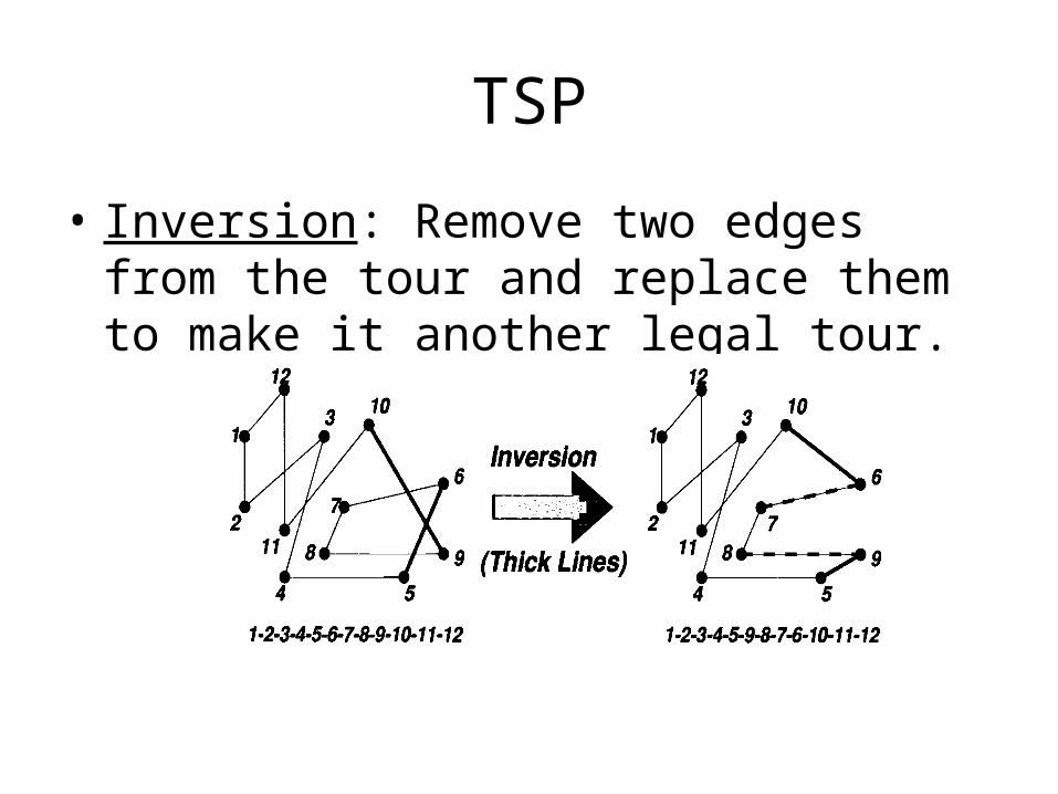
TSP

• Inversion: Remove two edges from the tour and replace them to make it another legal tour.

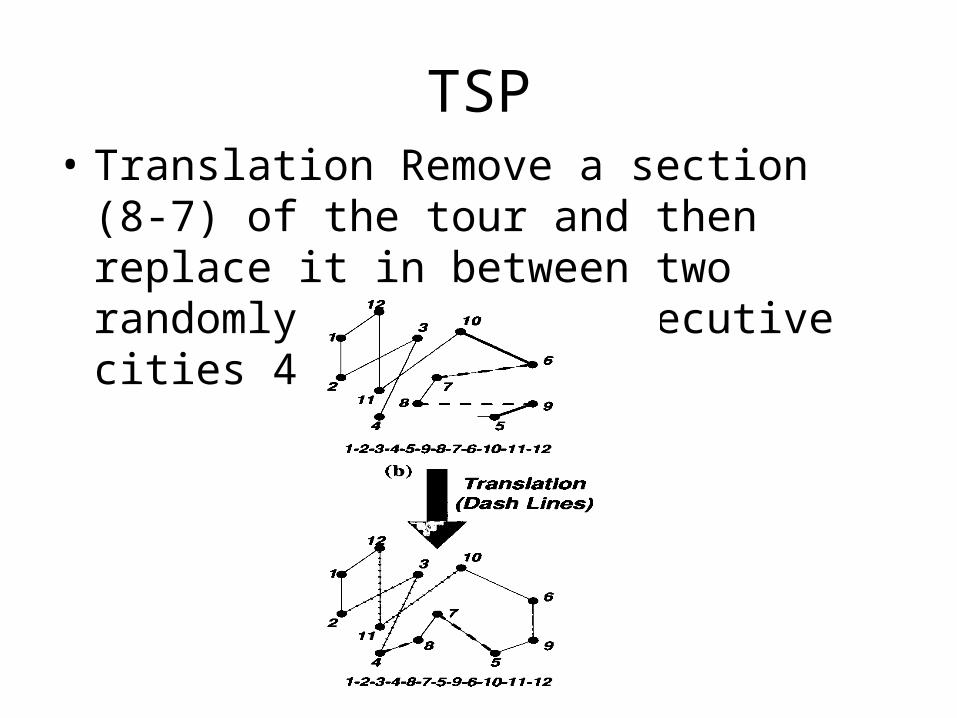
TSP• Translation Remove a section (8-7) of the tour

and then replace it in between two randomly selected consecutive cities 4 and 5).

TSP

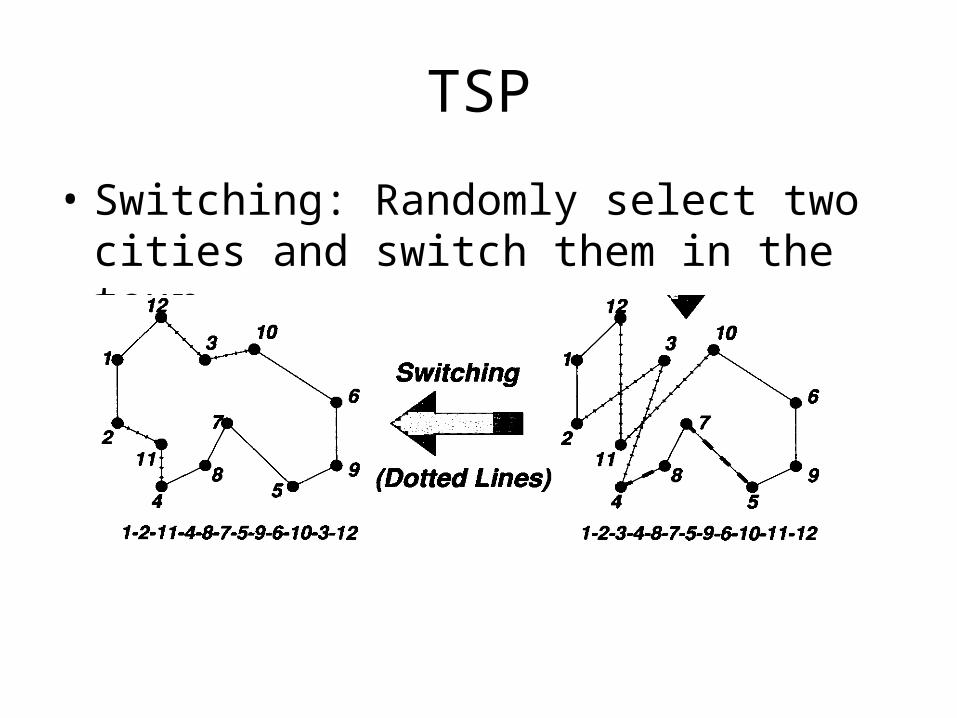
• Switching: Randomly select two cities and switch them in the tour

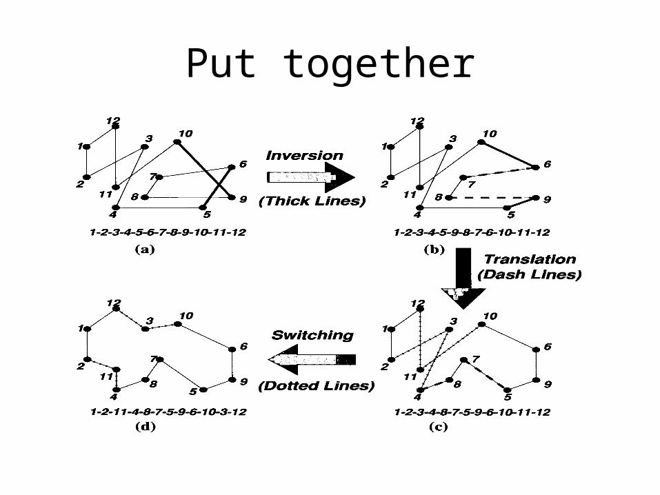
Put together

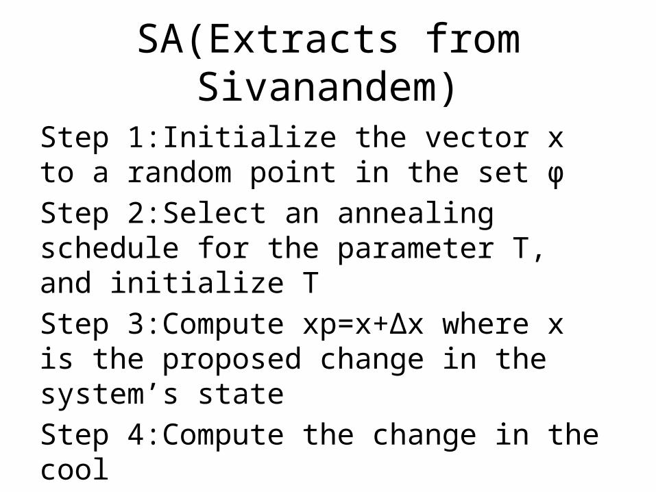
SA(Extracts from Sivanandem)

Step 1:Initialize the vector x to a random point in the set φStep 2:Select an annealing schedule for the parameter T, and initialize TStep 3:Compute xp=x+Δx where x is the proposed change in the system’s stateStep 4:Compute the change in the cool

Δf=f(xp)-f(x)

Algo contd….

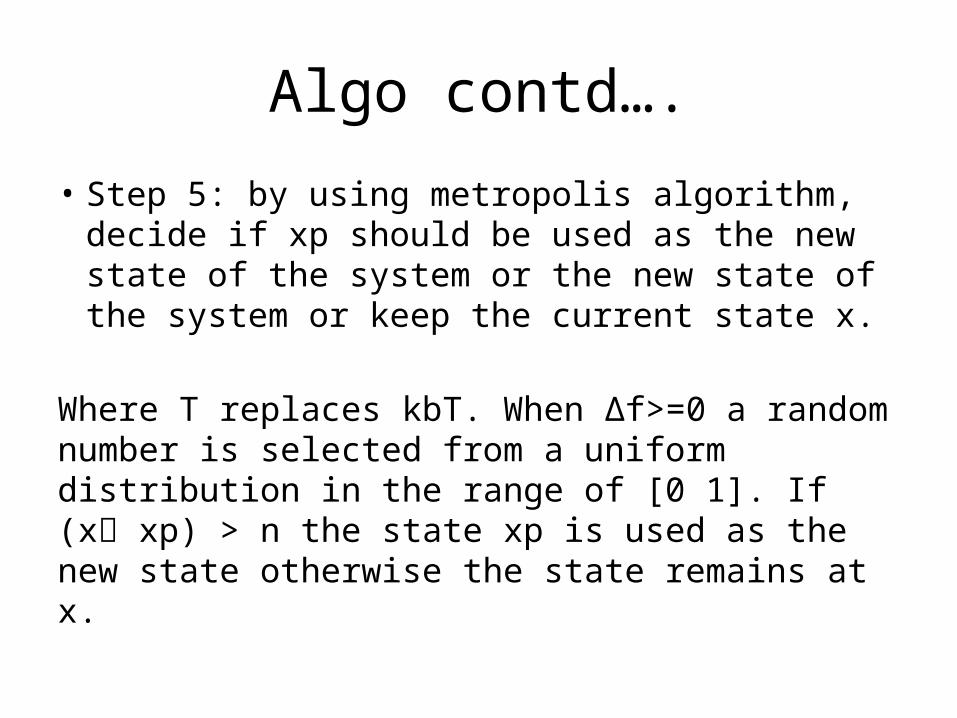
• Step 5: by using metropolis algorithm, decide if xp should be used as the new state of the system or the new state of the system or keep the current state x.

Where T replaces kbT. When Δf>=0 a random number is selected from a uniform distribution in the range of [0 1]. If (x xp) > n the state xp is used as the new state otherwise the state remains at x.

Algo contd….

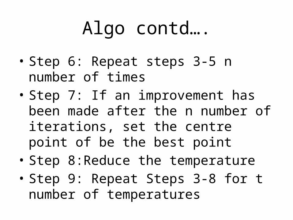
• Step 6: Repeat steps 3-5 n number of times• Step 7: If an improvement has been made

after the n number of iterations, set the centre point of be the best point

• Step 8:Reduce the temperature• Step 9: Repeat Steps 3-8 for t number of

temperatures

Random Search

• Explores the parameter space of an objective function sequentially in a random fashion to find the optimal point that maximizes or minimizes objective function

• Simple• Optimization process takes a longer time

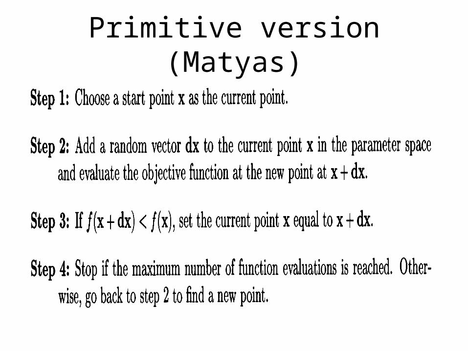
Primitive version (Matyas)

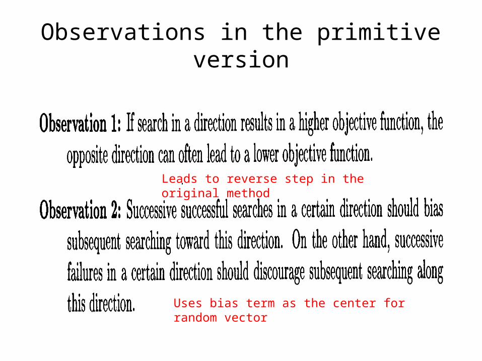
Observations in the primitive version

Leads to reverse step in the original method

Uses bias term as the center for random vector

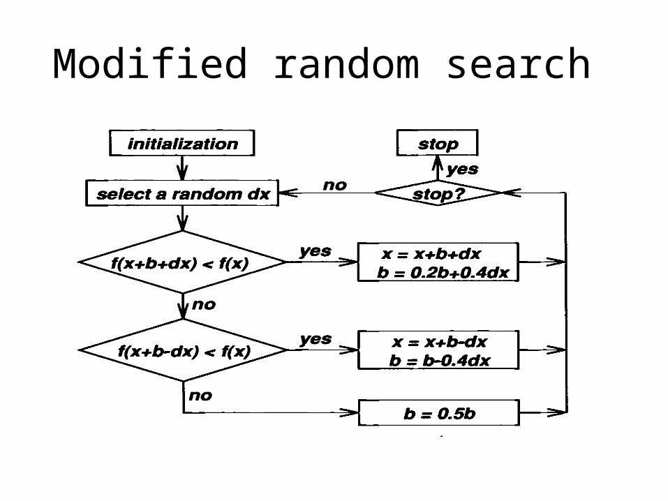
Modified random search

• Initial bias is chosen as a zero vector• Each component of dx should be a random

variable having zero mean and variance proportional to the range of the corresponding parameter

• This method is primarily used for continuous optimization problems