simulated annealing - diva portallnu.diva-portal.org/smash/get/diva2:608429/fulltext01.pdf ·...

Simulated Annealing For Large Scale Optimization inWireless Communications

Master Thesis Report in Electrical Engineering

Author: Tamim Sakhavat Haithem Grissa Ziyad Abdalrahman

Organisation: Faculty of TechnologyDate: 2013-02-20 Subject: Simulated AnnealingLevel: Master’s Course code: 5ED06E

Abstract

In this thesis a simulated annealing algorithm is employed as an optimiza-tion tool for a large scale optimization problem in wireless communication. Inthis application, we have 100 places for transition antennas and 100 places forreceivers, and also a channel between each position in both areas. Our aim isto find, say the best 3 positions there, in a way that the channel capacity ismaximized.

The number of possible combinations is huge. Hence, finding the best chan-nel will take a very long time using an exhaustive search. To solve this problem,we use a simulated annealing algorithm and estimate the best answer. The sim-ulated annealing algorithm chooses a random element, and then from the localsearch algorithm, compares the selected element with its neighbourhood.

If the selected element is the maximum among its neighbours, it is a localmaximum. The strength of the simulated annealing algorithm is its ability toescape from local maximum by using a random mechanism that mimics theBoltzmann statistics.

2

Contents

1 Simulated Annealing 61.1 Combinatorial Optimization Problem and Local Search . . . . . . 61.2 The Annealing Algorithm . . . . . . . . . . . . . . . . . . . . . . . . 81.3 Cooling Schedules . . . . . . . . . . . . . . . . . . . . . . . . . . . . 12

1.3.1 Initial Value for the Control Parameter . . . . . . . . . . . 121.3.2 Decrement of the Control Parameter . . . . . . . . . . . . . 131.3.3 Final Value for the Control Parameter . . . . . . . . . . . . 131.3.4 Length of Repetition . . . . . . . . . . . . . . . . . . . . . . 13

2 Channel Capacity 152.1 Channel . . . . . . . . . . . . . . . . . . . . . . . . . . . . . . . . . . 152.2 Channel Properties . . . . . . . . . . . . . . . . . . . . . . . . . . . . 162.3 Channel Capacity Formula . . . . . . . . . . . . . . . . . . . . . . . 16

3 MATLAB Codes 193.1 Basic Program for the Fix Temperature . . . . . . . . . . . . . . . 19

3.1.1 Algorithm . . . . . . . . . . . . . . . . . . . . . . . . . . . . . 193.2 Main Program . . . . . . . . . . . . . . . . . . . . . . . . . . . . . . 20

3.2.1 Temperature Algorithm . . . . . . . . . . . . . . . . . . . . 203.2.2 Main Program and Codes Explanation . . . . . . . . . . . 21

3.3 Functions . . . . . . . . . . . . . . . . . . . . . . . . . . . . . . . . . 243.3.1 Randomize . . . . . . . . . . . . . . . . . . . . . . . . . . . . 243.3.2 Skip Equality . . . . . . . . . . . . . . . . . . . . . . . . . . . 25

3.4 GUI . . . . . . . . . . . . . . . . . . . . . . . . . . . . . . . . . . . . . 263.4.1 GUI Appearance . . . . . . . . . . . . . . . . . . . . . . . . . 263.4.2 Simulated Annealing in GUI . . . . . . . . . . . . . . . . . 28

4 Plots and Results 314.1 Fix Temperature program . . . . . . . . . . . . . . . . . . . . . . . 314.2 Decreasing Temperature . . . . . . . . . . . . . . . . . . . . . . . . 32

5 References 38

Appendix A MATLAB Programs 39A.1 Program for Fix Temp . . . . . . . . . . . . . . . . . . . . . . . . . 39A.2 Program for Flexible Temp . . . . . . . . . . . . . . . . . . . . . . . 41

Appendix B Functions 43B.1 Randomize function . . . . . . . . . . . . . . . . . . . . . . . . . . . 43B.2 Skip Equality function . . . . . . . . . . . . . . . . . . . . . . . . . . 44

Appendix C GUI codes 45

3

Introduction

In some MIMO (multiple input multiple output) system, when there aredifferent choices to select for inputs or outputs, finding the best solution couldbe difficult.

For instance in this project, we have 100 places for transition antennas and100 places for receivers. Also there is an area between them, with objects andobstacles which caused scattering or fading of the signal. So we have a channelbetween each position in transition and receiving area. Our aim is to find thebest 3 positions here, in the way that, the fading and scattering of the signalbecome Minimum or in another word the SNR becomes Maximum. The numberof solution for this simple example, just for one area is defined from:

(100

3) =

100!

(100 − 3)!= 100 × 99 × 98 = 941288040000.

This is a very large number. So finding the best channels takes a lot of time.To solve this problem, one way is using the annealing simulation and estimatethe best answer.

Annealing is the physical process of heating up a solid until it melts, fol-lowed by cooling it down until it crystallizes into a state with a perfect lattice.[Simulated Annealing and Boltzmann machine by Emile Aarts and Jan Korst].The goal is reaching the ground state, where the energy of the solid is Minimum.

The annealing simulation chooses a random element, and then from the localsearch algorithm, compares the selected element with its neighborhood. If theselected element is the maximum in its neighbours, it will be chosen as the bestsolution, and then the same thing happens for the new element. The Boltzmannequation which is given below, help us to test other possibility when we stuckin a place, The Boltzmann equation is:

exp(Ei −Ej

KBT),

where Ei is the current state and Ej is the best tested solution. KB is theBoltzmann Constant and T defined as temperature. Then the probability ofselecting i as the best solution will be:

Pc(accept j) =

⎧⎪⎪⎨⎪⎪⎩

1, if Ej ≥ Ei

exp(Ei−Ejc

), if Ej < Ei.

We have four chapters in our report. In first chapter we try to explain simulatedannealing as much as we need for this report. Second chapter is a very basic

4

explanation about the channel capacity and the related formula.

And finally in the two last chapters, we use the Matlab software to simulatethe annealing method for our project and see the results. In the third chapter,first we assume that the temperature is fixed, and then by extending the resultfor flexible temperature, we can have a reasonable output.

And at the end we use Matlab GUI to make the program user friendly andeasy to use. A sample output is shown in the figure below:

As we can see, in this example, algorithm will find the best solution at thebeginning, around 15 [db]. But after a while by cooling down the system, theresult is improved and reached to 22 [db].

5

1 Simulated Annealing

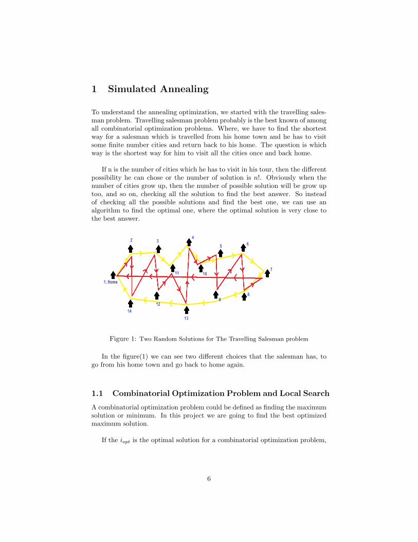
To understand the annealing optimization, we started with the travelling sales-man problem. Travelling salesman problem probably is the best known of amongall combinatorial optimization problems. Where, we have to find the shortestway for a salesman which is travelled from his home town and he has to visitsome finite number cities and return back to his home. The question is whichway is the shortest way for him to visit all the cities once and back home.

If n is the number of cities which he has to visit in his tour, then the differentpossibility he can chose or the number of solution is n!. Obviously when thenumber of cities grow up, then the number of possible solution will be grow uptoo, and so on, checking all the solution to find the best answer. So insteadof checking all the possible solutions and find the best one, we can use analgorithm to find the optimal one, where the optimal solution is very close tothe best answer.

Figure 1: Two Random Solutions for The Travelling Salesman problem

In the figure(1) we can see two different choices that the salesman has, togo from his home town and go back to home again.

1.1 Combinatorial Optimization Problem and Local Search

A combinatorial optimization problem could be defined as finding the maximumsolution or minimum. In this project we are going to find the best optimizedmaximum solution.

If the iopt is the optimal solution for a combinatorial optimization problem,

6

then we can formalized the problem to:

⎧⎪⎪⎨⎪⎪⎩

Maximization, f(iopt) ≥ f(i) for all i ∈ S

Minimization, f(iopt) ≤ f(i) for all i ∈ S.

Where fopt = f(iopt) denotes the optimal cost, and Sopt the set of optimalsolutions.

The next step is Local Search. When we searching for the solution, and welook around the neighbourhood of the previous guessing solution, the approxi-mation of the best solution will be decrease considerably.

The algorithm start from the very randomly solution, then the algorithmsearch its neighbourhood to find the better solution. The next step would bereplacement of the new solution into the old one, in the case of finding a bettersolution. And it goes until there wasn’t any better solution in a neighbour ofthe existent one. The last solution would be the optimal solution for a combi-natorial optimization problem. The following definition will explain local search.

Definition 1.1: Let (S, f) be an instance of a combinatorial optimizationproblem and let N be a neighbourhood structure, then i ∈ S is called a locallyoptimal solution or simply a local optimum with respect to N if i is betterthan, or equal to, all its neighbouring solutions with regard to their cost. Morespecifically, in the case of minimization, i is called a locally minimal solution orsimply a local minimum if:

f (i) ≤ f(j), for all j ∈ Si

and in the case of maximization, i is called a locally maximal solution orsimply a local maximum if

f (i) ≥ f(j), for all j ∈ Si

See [1, Chapter. 1 - page. 8] ∎

In the codes below we can see the MATLAB® program for local search al-gorithm.

i = ” i n i t i a l va lue for s t a r t ” ;N = ” Last Members o f the Neighbourhood ” ;for j =1:N

i f f ( i ) < f ( j ) ;i=j ;

endend

7

The most important things in a local search for combinatorial optimizationproblem are initial value for starting and which algorithm we use to chose ran-domly the neighbourhood.

The best feature of simulated annealing algorithm is the optimal solution isnot depended strongly to the initial value nor the randomly algorithm of choos-ing the neighbourhood.

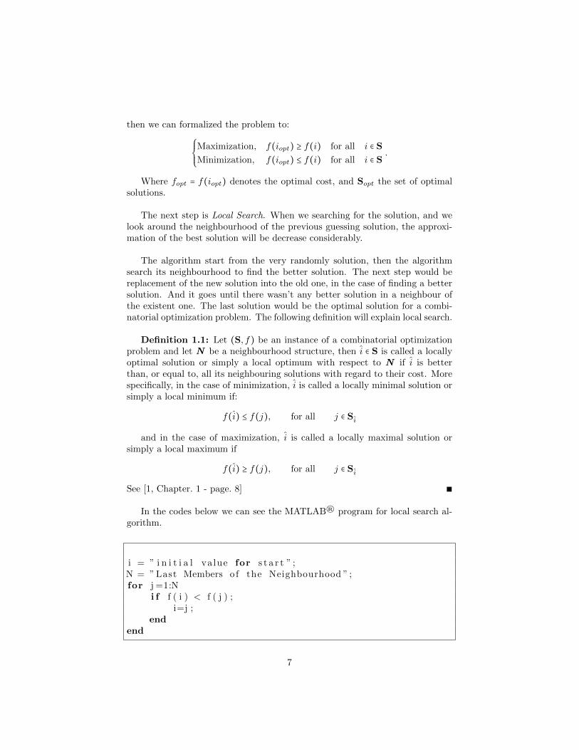
In the figure (2), we can see how local search algorithm, is to be able to findthe maximum number in the matrix after three steps.

Figure 2: Finding The Maximum, Using Local Search

The major problem in local search is, the algorithm may stocks in a neigh-bour with a solution, but the solution is not the maximum nor enough close toit. In the next section we will introduce a control parameter which will help usto avoid this sort of situation.

1.2 The Annealing Algorithm

Annealing, which is known as a thermal process for obtaining low energy statesof solid in heat bath, contains two steps:

- Heat up the solid until it melts.

- Decrease carefully the temperature until the particles change to the crystalby itself.

The goal is, the whole process has to reach to the ground state1 in the end.The ground state happens just when the cooling down goes very slowly.

1The Ground state is the state when the energy of the particle is Minimum.

8

The main different between the Annealing algorithm and Local search is, inLocal search, as we mention before, we don’t have any control on the systemduring the search or process. The cooling happens randomly and after a whileit will be stopped. But in Annealing algorithm in addition to choose randomlyfrom the neighbourhood of the solution we have a control parameter. The con-trol parameter helps the algorithm to go out of the trap. In normal Local search,if the current solution is the optimal solution on its neighbourhood, the processwill be stop, whereas there are still much better solution around. This case isusually called the trap. The way to get out of the trap is choosing a controlparameter, and check the current solution with more different cases.

In the Metropolis algorithm for annealing simulation, the control parameteris temperature. If we show the energy of the state i with Ei and the energy ofstate j with Ej , then Ei −Ej is the energy difference between state i and j. Ifthe energy difference is less than or equal to zero, state j will be accepted asthe best state solution, otherwise the state j still have a chance to be chosen asthe best solution with a certain probability of

exp(Ei −Ej

kBT), (1)

where T is the temperature of the heat bath and kB would be the Boltzmannconstant.

If X is a stochastic variable denoting the current state of the solid, and Z(T )

is the partition function. Then the probability for the solid to be in the sate iwill be calculated as

PT (X = i) =1

Z(T )exp(

−Ei

kBT), (2)

where Z(T ) is

Z(T ) =∑(exp(−Ei

kBT)). (3)

Convincingly, we can say the annealing algorithm is followed by the metropo-lis algorithm, when a sequence of solution for a combinatorial problem will berequest. There are two equivalents here. First, states of physical system are thesolution for the problem, and secondly the energy of state is the cost of solution.

The definition 2.1 will show us how annealing algorithm works.

Definition 2.1: Let (S, f) denote an instance of a combinatorial optimiza-tion problem and i and j are two solutions with cost f(i) and f(j), respectively.

9

Then the acceptance criterion determines whether j is accepted from i by ap-plying the following acceptance probability:

Pc(accept j) =

⎧⎪⎪⎨⎪⎪⎩

1, if f(j) ≤ f(i)

exp( f(i)−f(j)c

), if f(j) > f(i), (4)

where c ∈R+ denotes the control parameter.

Clearly, the generation mechanism corresponds to the perturbation mecha-nism in the metropolis algorithm, where the acceptance criterion correspondsto the metropolis criterion.See [1, Chapter. 2 - page. 15]. ∎

By the definition and if L denotes the number of transition, c is the controlparameter, and i,j are two possible solutions for the annealing problem, then asimple MATLAB® code for generating an optimum solution could be:

for i =1:Li f f ( i ) <= f ( j ) ;

i = j ;e l s e i f exp ( ( f ( i )− f ( j ) ) /c ) > rand ;

i = j ;end

end

As we can see in the equation (No. 1), for the large c, the whole exponentialis very small, so the possibility of acceptance of the solution in the second step

is very large. But as c decreases, the exp( f(i)−f(j)c

), increase to 1 (the powergoes to infinity). And again from the second condition in definition 4.1 , thepossibility of acceptance of the solution goes to zero. And finally when c is zero,all the solution must satisfied the first condition.

From the basic of stochastic distribution we have the definition (2.2).

Definition 2.2:

1. The expected cost Ec(f) is equal to:

Ec(f)def= ⟨f⟩c =∑

i∈S

f(i)P(X = i) =∑i∈S

f(i)qi(c). (5)

2. And then the expected square cost Ec(f2) would be:

Ec(f2)

def= ⟨f2

⟩c =∑i∈S

f2(i)P(X = i) =∑

i∈S

f2(i)qi(c). (6)

10

3. The variance Varc(f) of the cost function or σ2c is:

Varc(f)def= σ2

c =∑i∈S

(f(i) −Ec(f))2P(X = i)

=∑i∈S

(f(i) − ⟨f⟩c)2qi(c) = ⟨f2

⟩c − ⟨f⟩2c = σ2c . (7)

4. And finally the entropy2 is calculated from:

S c = −∑i∈S

qi(c) ln qi(c). (8)

∎

And The following results is also useful to understand the consent of anneal-ing optimization better.

Definition 2.3:

1.

limc→∞

⟨f⟩cdef= ⟨f⟩∞ =

1

∣S∣∑i∈S

f(i). (9)

2.limc→0

⟨f⟩cdef= fopt. (10)

3.limc→∞

σ2c

def= σ2

∞ =∑i∈S

(f(i) − ⟨f⟩∞)2. (11)

4.limc→0

σ2c = 0. (12)

5.limc→∞

Scdef= S∞ = ln ∣S∣. (13)

6.limc→0

Scdef= S0 = ln ∣Sopt∣. (14)

∎

To see the proofs and more information about the (Definition 2.3 ) check thebook Simulated annealing and Boltzmann Machines chapter 2.[1]

2The entropy is a natural measure of amount of disorder or information in a system.

11

1.3 Cooling Schedules

In simulated annealing choosing a cooling schedule would be the most impor-tant thing to do. By choosing the best control parameter, the best decrementvalue for temperature and etc... we can have a fast and efficient way to reachour goal, which is locally optimal cooling structure with crystal imperfections.in this section we try to explain very briefly about this important components.

Definition 3.1:A cooling schedule specifies:

- An initial value of the control parameter.

- A decrement function for decreasing the value of the control parameter

- A final value of the control parameter specified by stop criterion

- A finite length of each homogeneous repetition.

[1, Chapter. 4 - page. 57] ∎

1.3.1 Initial Value for the Control Parameter

A very important element in cooling Schedules is acceptance ratio. The accep-tance ratio is defined in the following definition.

Definition 3.2: The acceptance ratio χ(c) in the simulated annealing algo-rithm is defined as:

χ =number of accepted transitions

number of proposed transitions∣c. (15)

∎

If c0 denotes the initial value for the control parameter, then for mostlyaccepted transition by the system the c0 should be large enough, but we haveto be careful because if c0 was too large then, the time for cooling down willbe increase. For this reason the acceptance ratio χ0 = χ(c0) should be close to 1.

It can be calculated in reality by choosing a very small value for c0 andmultiplying it by a constant grater than 1 and reach the point which χ0 = χ(c0)is close to 1 enough. But for be more specific and practical, we also can use thefollowing formula:

χ ≈m1 +m2.exp(

−∆(f)+

c)

m1 +m2, (16)

and c will be calculated from:

c =∆(f)

+

ln( m2

m2.χ−m1(1−χ)), (17)

12

where m1 and m2 are the numbers of transitions from i to j when f(i) onthe condition:

⎧⎪⎪⎨⎪⎪⎩

m1 if f(i) ≥ f(j)

m2 if f(i) < f(j),

and (−∆(f)+) would be an average difference in cost over m2 cost increasing

transitions.

For start we can put the zero as the initial value for c0 and start the loop tocalculate the sequences. The following value for m1, m2 , χ will be calculatedfrom the c0 then. For more details check the book Simulated Annealing andBoltzmann Machines by Emile Aarts [1].

1.3.2 Decrement of the Control Parameter

In general the decrement of the control parameter could be calculate from themultiplying a number in to c:

ck+1 = α.ck , k = 1,2, ...,

where α is a constant number close to 1, and usually it’s number between 0.8and 0.99. But for more details we bring the following definition which we cancalculate the exact value for decrementing of the control parameter.

1.3.3 Final Value for the Control Parameter

The value for the control parameter depends on an extrapolation of the expectedcost function when ⟨f⟩ck goes to zero. Then we estimate the final value by using∆⟨f⟩c. So we have

∆⟨f⟩c = (⟨f⟩c − fopt) ≈ cδ⟨f⟩cδc

, (18)

ck⟨f⟩∞

∆⟨f⟩cδc

∣c=ck < εs. (19)

The εs should be a very small, positive number.

1.3.4 Length of Repetition

By choosing the right control parameters and Start and Stop temperature wecan do the cooling down in the shortest time. From the equation below we cancalculate a coefficient to control the speed of the process for cooling down.

Tstop = Tstart × aq, (20)

then:log(Tstop) = log(Tstart) + q log(a), (21)

13

so:

a = 10(log(

TstopTstart

)

q). (22)

The equation (No. 22), is the temperature coefficient which we will use laterto cool down the system.

14

2 Channel Capacity

A channel in signal processing antenna is a path between transition and receiverelements. Each path has it’s own characteristic feature , like gain, fading, scat-tering and etc. In general, this features are called Capacity. In this chapter wewill explain this meaning as far as we need. For more information check Fun-damentals of Wireless Communication by David Tse and Pramod Viswanath.

2.1 Channel

A system in signal processing is a collection of components together which hasthe same physical behaviour. And any cost function which has data or infor-mation about a specific system is called signal.

The MIMO system or Multiple Input, Multiple Output is a system with morethan one input and output signal. In antenna area, the MIMO is also calledMEAs or in some books MEA which is stand for Multiple Elements Antennasystem. In the figure(3) we can see a sample of MIMO system.

Figure 3: MIMO Sample Channel

As we can see in the figure, it’s not important that the number of inputsignal and output signal be equal and also it’s possible that two input signaleffect one output or more. A system could be an area between to antenna whichactually is a path for signal to reach the reviver antenna. This system is calledchannel.

15

2.2 Channel Properties

There are a lot of things where will be effected the capacity of channel like scat-tering, diffraction, infraction which are predictable and also in addition thereare some unpredictable things. We call these unpredictable things, noise. Thenoise is a undesired and unwanted energy (electrical or electromagnetic) whichreduce and effect the quality of the signal in the output. In real life the noise isa random signal which will be added to the desired signal.

Assume that the Tr is period of the time when the channel receive the newinformation or data. And Ts is the period of time when the channel will spendto send the data to the output. Now if the H(s) is the entropy of the system.Then the bit rate of the channel will be given by, (Br) and it equal to:

Br =H(s)TsTr

. (23)

From the bit rate of the channel, we can define another definition for capacityof the channel. The capacity of the channel is the maximum data we will see inthe output without error, or with a negligible error. Now if the bandwidth ofthe channel is ω and Tr is still as before, then we can say:

Tr =1

2ω. (24)

With equation (24), the capacity of the channel is measured in data bitsper second. In addition if X and Y are two random variable and H(X ∣Y ) is aconditional entropy then the capacity of channel will be defined as:

C = max I(X;Y ) where I(X;Y ) =H(Y )H(Y ∣X). (25)

where H is the channel properties and X and Y is input and output of thechannel respectively.

2.3 Channel Capacity Formula

When we are modelling the channel, to approach the better result and have morecontrol on that, the system should be LTI3. And for this reason we assume thatthe signal is narrow banded, it means the signal wouldn’t change a lot duringthe time. In general we show the relation between input/output for a narrowband signal in any MIMO system, with the complex numbers as follow:

y =H(x) + n. (26)

So if y is a receive signal which will be show by (N × 1) matrix and x whichis the output and we denote it by a (M × 1) matrix, then H as the channel will

3Linear, Time invariant

16

be a matrix with M input signal and N output and will be shown by a (M ×N)matrix. And n in the equation (26) is white Gaussian noise and its dimensionshould be the same as the output, which is (N × 1).

To have the receiver with the perfect channel knowledge, we assume thatthe channel matrix is random and memoryless4.

Now we can write the matrix for the MIMO channel. The H matrix thatdenote the channel has (M×N) elements and notice that each element is complexnumber. It means it has a real part and imaginary part both. If each elementwill be given as hmn then the channel matrix H will be shown as:

⎡⎢⎢⎢⎢⎢⎣

h11 ⋯ h1N

⋮ ⋱ ⋮

hM1 ⋯ hMN

⎤⎥⎥⎥⎥⎥⎦

(27)

and each complex element would be given by:

hmn = α + iβ or hmn =√α2 + β2 × e−iarctan(αβ ). (28)

SISO5 is a channel where M = N = 1. The capacity of a SISO channel isthe maximum of the information between the input signal and the output forall distributions which satisfied the condition. Now if Signal to Noise Ratio willbe denoted by SNR then the capacity for the SISO channel will be given by:

C = EH{log2(1 + SNR.∣h11∣2)}, (29)

where EH is the expectation for all channel. As we can see because thechannel has one input, and one output, then the Matrix has just one elementh11.

But in MIMO channel, the matrix H has more than one element, So therelated formula for channel capacity in this case will be defined as:

C = EH{log2[det(InR +PTσ2nT

HHH)]}. (30)

Here, PT is the transited power and nT is the number of transition antennas.We can rewritten the equation (No. 30) to:

C = EH{log2[det(InR +ρ

nTHHH

)]}, (31)

where ρ is the PTσ2 .

4the capacity can be computed as the maximum of the information5Single Input, Single Output channel

17

The covariance6 matrix for input signal will be denoted as:

σ2x =

PTnT

InT . (32)

We usually assume the noise and the desired signal are uncorrelated. In gen-eral and after some calculation and estimation we will reach the main formulafor capacity of channel. Assume that the (m×n) H channel matrix with whiteGaussian noise. Then if n was the number of antenna at reviver at transitionarea, then the capacity of channel will be given by:

C = log2 det(I +SNR

nHHH

), (33)

where I is the (m×m) identity matrix, and SNR is the signal to noise ratio.

6σ2c or Cov(x) of the matrix is (XXH) and H means Hermitian of the matrix.

18

3 MATLAB Codes

In this chapter first we use the MATLAB® software to simulated the Annealingmethod for the (3×3) random places in a (100×100) positions of antennas. Thenby extending the result to any desire numbers for antennas in any area with anypossibility of number for solutions we will give the reader a good perspective ofhow the simulated Annealing should work. We also try to separate the wholeprogram to smaller part and Functions. And in the end we use the MATLABGUI® to make the program more user friendly and easier to use.

3.1 Basic Program for the Fix Temperature

We have two sort of algorithms for annealing estimation, first, use the algorithmin the specific temperature, which we call it FIX Temperature, and second onefor cooling down system, when temperature start at very high degree and endedin its lowest point. In this chapter we will talk about the FIX temperaturealgorithm.

3.1.1 Algorithm

As we explain before, first we start with very basic program, with a fix givingtemperature, fix input/output number of signals and fix number of positions forchannel.

Before we go through the program, notice that to create a random channel,instead of using “rand” we use “randn”. The main different between rand andrandn is, the rand code in MATLAB® will create a random number between0 and 1 but randn is a “normally (Gaussian) distributed random number gen-erator”. The reason to use randn is, in any telecommunication channel, wehave The white noise, and the white noise has the normally (Gaussian) distri-bution elements and these elements will be added to the elements of the channelcharacters. So by using the randn we can simulate the channel, more realistic.Anyway, the programs that we write for this reason is given in the appendix(A.1).

In this program, algorithm will calculate the capacity of the given channel(which here it is [100×100] random channel) and plot the capacity for (3×3) bestpositions in the end. As we can see in appendix (A.1) the noise power assumeis 1 and signal power is given 10. K which is the test repetition is 100000. Inthe follow we show outputs, for different temperatures.

19

3.2 Main Program

By Main we mean the algorithm which works for decreasing temperature anddo the estimation for K different times.

3.2.1 Temperature Algorithm

Before we write the program for simulated annealing, lets talk a little abouthow temperature has to change during the repetition.

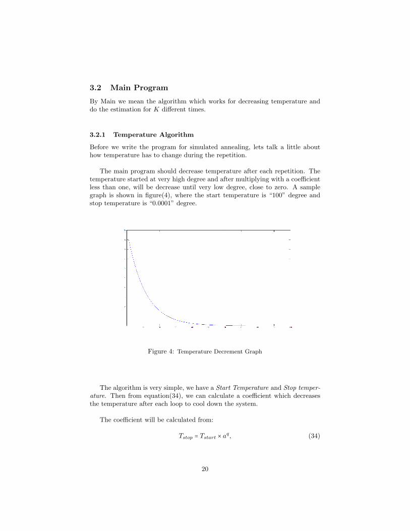
The main program should decrease temperature after each repetition. Thetemperature started at very high degree and after multiplying with a coefficientless than one, will be decrease until very low degree, close to zero. A samplegraph is shown in figure(4), where the start temperature is “100” degree andstop temperature is “0.0001” degree.

Figure 4: Temperature Decrement Graph

The algorithm is very simple, we have a Start Temperature and Stop temper-ature. Then from equation(34), we can calculate a coefficient which decreasesthe temperature after each loop to cool down the system.

The coefficient will be calculated from:

Tstop = Tstart × aq, (34)

20

where Tstart and Tstop are start and stop temperatures, q is the steps ofdecreasing or in another words, how fast the curve of temperature graph shouldreach to zero. And finally a is the coefficient which we are looking for. So wehave:

log(Tstop) = log(TStart) + q log(a)

log(a) =log(Tstop) − log(TStart)

q

log(a) =log(

TstopTStart

)

q

a = 10log( Tstop

TStart)

q , (35)

and a, in the equation (3.2.1) is the coefficient which we used in the program.

3.2.2 Main Program and Codes Explanation

We can see the MATLAB® program for annealing algorithm in appendix (A.2).We explain each part separately in the follow:

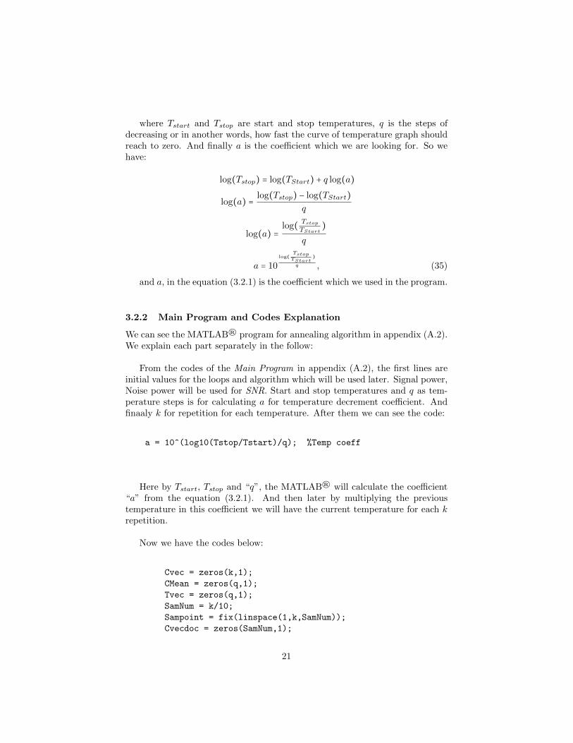
From the codes of the Main Program in appendix (A.2), the first lines areinitial values for the loops and algorithm which will be used later. Signal power,Noise power will be used for SNR. Start and stop temperatures and q as tem-perature steps is for calculating a for temperature decrement coefficient. Andfinaaly k for repetition for each temperature. After them we can see the code:

a = 10^(log10(Tstop/Tstart)/q); %Temp coeff

Here by Tstart, Tstop and “q”, the MATLAB® will calculate the coefficient“a” from the equation (3.2.1). And then later by multiplying the previoustemperature in this coefficient we will have the current temperature for each krepetition.

Now we have the codes below:

Cvec = zeros(k,1);

CMean = zeros(q,1);

Tvec = zeros(q,1);

SamNum = k/10;

Sampoint = fix(linspace(1,k,SamNum));

Cvecdoc = zeros(SamNum,1);

21

The first three lines are:

- The Capacity vector for the channel after each repetition.

- Mean value for the capacity of the channel.

- Time vector for each repetition.

Then at the fourth line we sampling by 110

of the Capacity vector to makeit smaller vector to be able to plot it later. Just to be more clear why we haveto do that, imagine that the k, repetition is 1000 and q temperature steps is10000, then the output vector for capacity will have 1000 × 10000 = 10000000elements. But after sampling 1

100we have 10000000

100= 100000, which is quite

smaller than the original. Obviously we can change the number of sampling ifthe input numbers for k and q are not that much high, like here in this programwe use 1

10sample instead of 1

100.

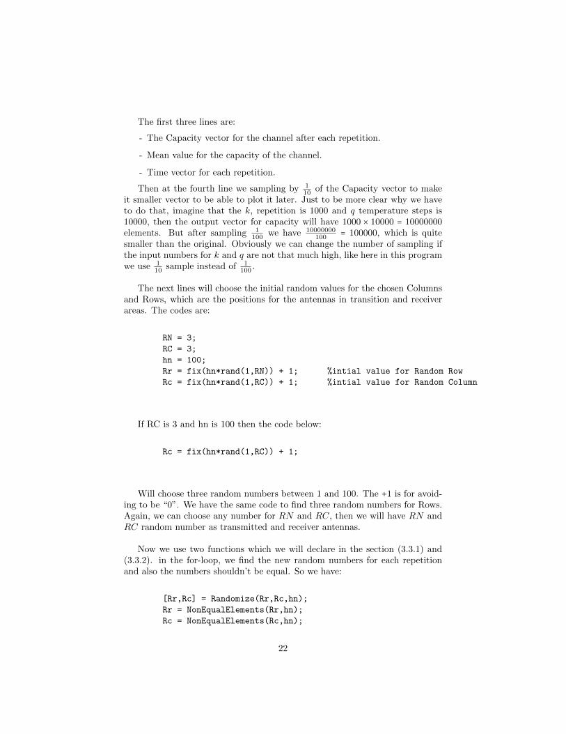
The next lines will choose the initial random values for the chosen Columnsand Rows, which are the positions for the antennas in transition and receiverareas. The codes are:

RN = 3;

RC = 3;

hn = 100;

Rr = fix(hn*rand(1,RN)) + 1; %intial value for Random Row

Rc = fix(hn*rand(1,RC)) + 1; %intial value for Random Column

If RC is 3 and hn is 100 then the code below:

Rc = fix(hn*rand(1,RC)) + 1;

Will choose three random numbers between 1 and 100. The +1 is for avoid-ing to be “0”. We have the same code to find three random numbers for Rows.Again, we can choose any number for RN and RC, then we will have RN andRC random number as transmitted and receiver antennas.

Now we use two functions which we will declare in the section (3.3.1) and(3.3.2). in the for-loop, we find the new random numbers for each repetitionand also the numbers shouldn’t be equal. So we have:

[Rr,Rc] = Randomize(Rr,Rc,hn);

Rr = NonEqualElements(Rr,hn);

Rc = NonEqualElements(Rc,hn);

22

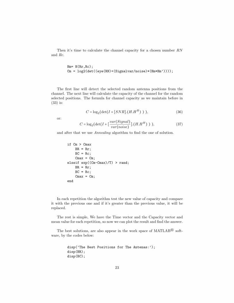
Then it’s time to calculate the channel capacity for a chosen number RNand Rc.

Hm= H(Rr,Rc);

Cm = log2(det((eye(RN)+(Signalvar/noise)*(Hm*Hm’))));

The first line will detect the selected random antenna positions from thechannel. The next line will calculate the capacity of the channel for the randomselected positions. The formula for channel capacity as we maintain before in(33) is:

C = log2(det(I + [SNR].(H.HH) ) ), (36)

or:

C = log2(det(I + [var(Signal)

var(noise)].(H.HH

) ) ), (37)

and after that we use Annealing algorithm to find the one of solution.

if Cm > Cmax

BR = Rr;

BC = Rc;

Cmax = Cm;

elseif exp((Cm-Cmax)/T) > rand;

BR = Rr;

BC = Rc;

Cmax = Cm;

end

In each repetition the algorithm test the new value of capacity and compareit with the previous one and if it’s greater than the previous value, it will bereplaced.

The rest is simple, We have the Time vector and the Capacity vector andmean value for each repetition, so now we can plot the result and find the answer.

The best solutions, are also appear in the work space of MATLAB® soft-ware, by the codes below:

disp(’The Best Positions for The Antenas:’);

disp(BR);

disp(BC);

23

The plots and results are explained in the next chapter.

3.3 Functions

MATLAB® functions are some .m files which will be used more frequently inother codes and programs. Here we create two functions to make the programsimpler to use. these two functions are used to randomize the input/outputelements and to skip choosing the same element for the inputs/outputs, if thenumber of selection is more than one.

3.3.1 Randomize

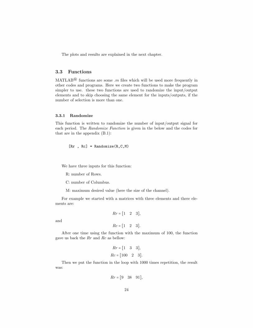
This function is written to randomize the number of input/output signal foreach period. The Randomize Function is given in the below and the codes forthat are in the appendix (B.1):

[Rr , Rc] = Randomize(R,C,M)

We have three inputs for this function:

R: number of Rows.

C: number of Columbus.

M: maximum desired value (here the size of the channel).

For example we started with a matrices with three elements and there ele-ments are:

Rr = [1 2 3],

andRc = [1 2 3].

After one time using the function with the maximum of 100, the functiongave us back the Rr and Rc as bellow:

Rr = [1 3 3],

Rc = [100 2 3].

Then we put the function in the loop with 1000 times repetition, the resultwas:

Rr = [9 38 91],

24

Rc = [94 84 36].

And we have completely different random number, between 1 and 100.

3.3.2 Skip Equality

Just because we couldn’t have the same Column’s or Row’s elements in the out-put for our algorithm, we write the following function to skip that. The relatedcodes for this function is in appendix (B.2).

RM = NonEqualElements(M,hn)

We have two inputs. One is our vector and another one is the maximumpossible value for each elements. For example imagine a vector with 10 elements,and all of them are 1 as below:

R = [ 1 1 1 1 1 1 1 1 1 1 ].

After using the function the result for R as above and the maximum possiblevalue for each element equal to 100 will be:

R = [ 1 44 82 51 70 37 49 63 55 66 ].

25

3.4 GUI

GUI 7 is a library in MATLAB®, for presentations and make the codes moreuser friendly. In this section we explain how it works and then we explain ourGUI in this project.

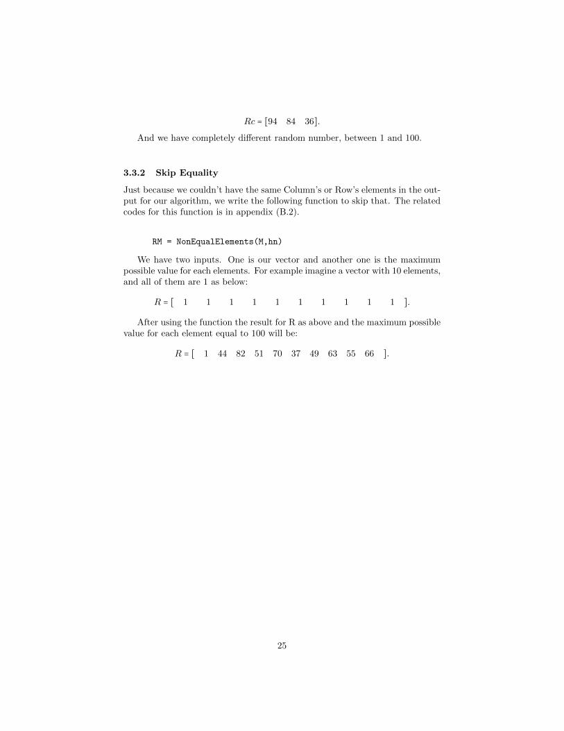
3.4.1 GUI Appearance

After running the MATLAB® software, on the top of the Main window thereis an Icon with the shape of pen in it, right beside the Simulink icon.

We can use the GUI feature by pushing this button or writing GUIDE inthe command window. After doing that, a new window will be appear.

7Graphical User Interface

26

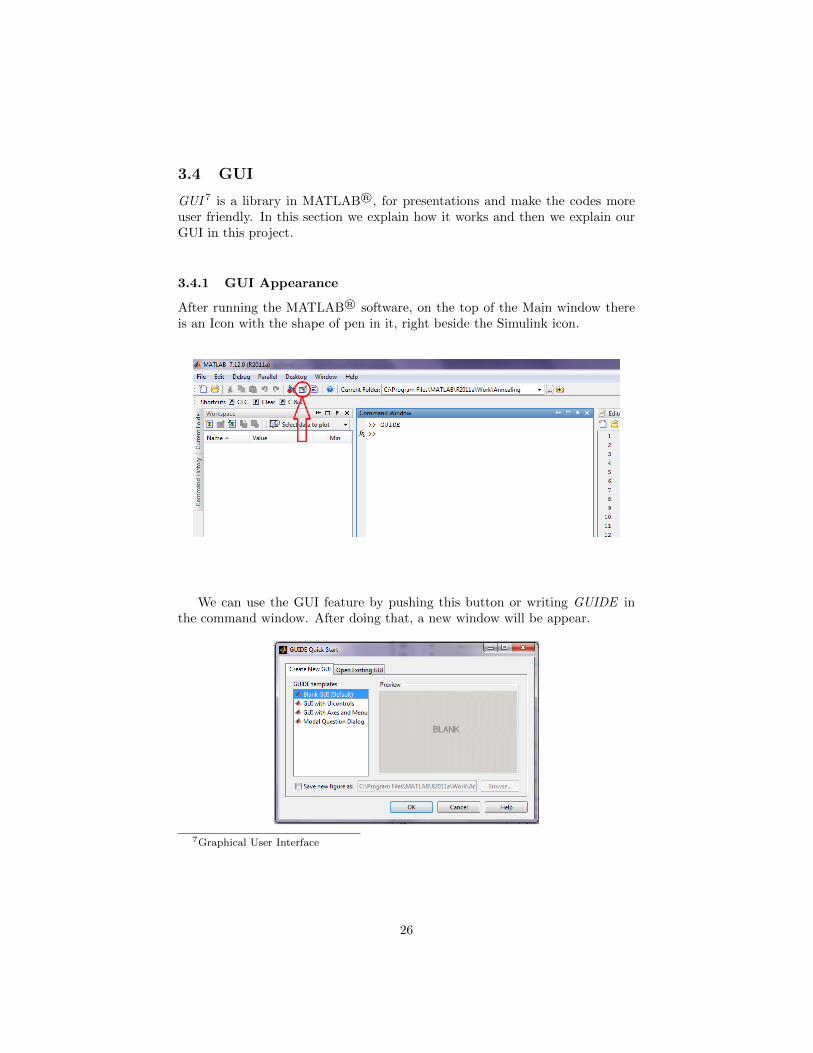
In this window you can choose what type of GUI do you need to work with,Or choose from a list which you have already made.

To start, we choose the Blank GUI from the first menu. The new windowwill be made, with the name (untitled.fig).

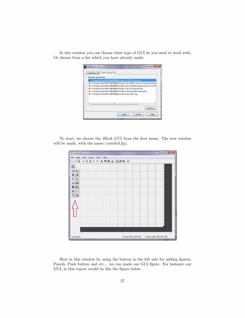
Here in this window by using the button in the left side for adding figures,Panels, Push button and etc... we can made our GUI figure. For instance ourGUI, in this report would be like the figure below.

27

By Double clicking on each selected box, in this window, the Inspector win-dow for the related box will be shown, where you can edit everything of theselected box in GUI, like the colour, size, place of the box in the whole plateand etc.

After putting everything in the right place, now you have to save the figure.By saving the figure, MATLAB® will create a .m file, where every buttonsand boxes have a definition and codes. Now we have to back to our GUI.fig,and right click on the target button or any box, and from the pop up menu,choose “View Callback” → “Callback”.MATLAB® will go to the .m file whichis already made and show the place that you have to add the related codes forthat button.

The next time you want to run the GUI, you just need to run the programlike any other .m files. MATLAB® will show the GUI window by itself. To editit again, go to the GUI button on the top of the main window or easily writeGUIDE in the command window.

3.4.2 Simulated Annealing in GUI

We just explain about how to make a GUI window, button, and etc. So in thissection we just give the reader some explanation about what does each buttondo in our GUI window and how to plot the desired figure.

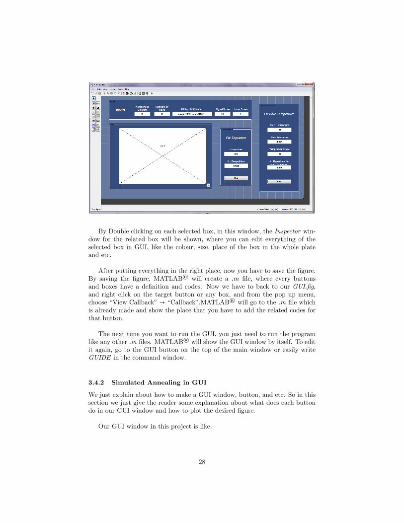
Our GUI window in this project is like:

28

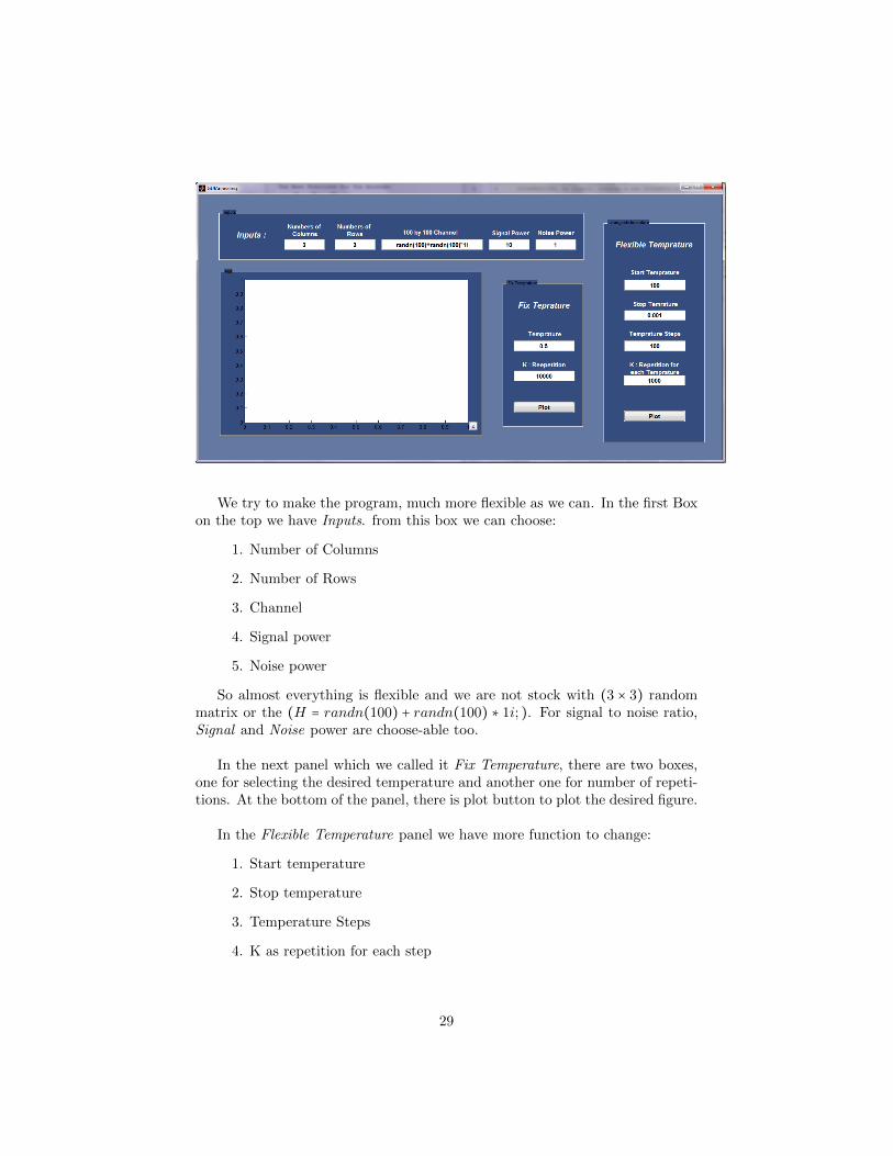
We try to make the program, much more flexible as we can. In the first Boxon the top we have Inputs. from this box we can choose:

1. Number of Columns

2. Number of Rows

3. Channel

4. Signal power

5. Noise power

So almost everything is flexible and we are not stock with (3 × 3) randommatrix or the (H = randn(100) + randn(100) ∗ 1i; ). For signal to noise ratio,Signal and Noise power are choose-able too.

In the next panel which we called it Fix Temperature, there are two boxes,one for selecting the desired temperature and another one for number of repeti-tions. At the bottom of the panel, there is plot button to plot the desired figure.

In the Flexible Temperature panel we have more function to change:

1. Start temperature

2. Stop temperature

3. Temperature Steps

4. K as repetition for each step

29

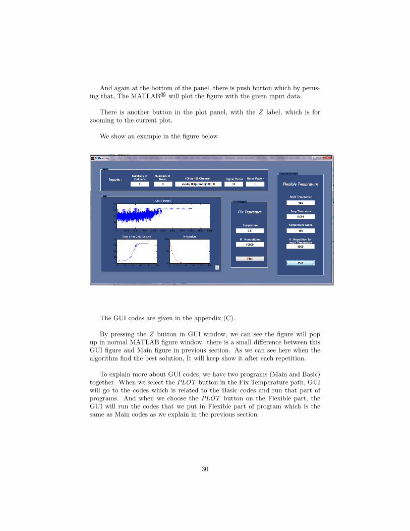
And again at the bottom of the panel, there is push button which by perus-ing that, The MATLAB® will plot the figure with the given input data.

There is another button in the plot panel, with the Z label, which is forzooming to the current plot.

We show an example in the figure below

The GUI codes are given in the appendix (C).

By pressing the Z button in GUI window, we can see the figure will popup in normal MATLAB figure window. there is a small difference between thisGUI figure and Main figure in previous section. As we can see here when thealgorithm find the best solution, It will keep show it after each repetition.

To explain more about GUI codes, we have two programs (Main and Basic)together. When we select the PLOT button in the Fix Temperature path, GUIwill go to the codes which is related to the Basic codes and run that part ofprograms. And when we choose the PLOT button on the Flexible part, theGUI will run the codes that we put in Flexible part of program which is thesame as Main codes as we explain in the previous section.

30

4 Plots and Results

In this chapter we will give you the output of the programs and then we willexplain each plot separately.

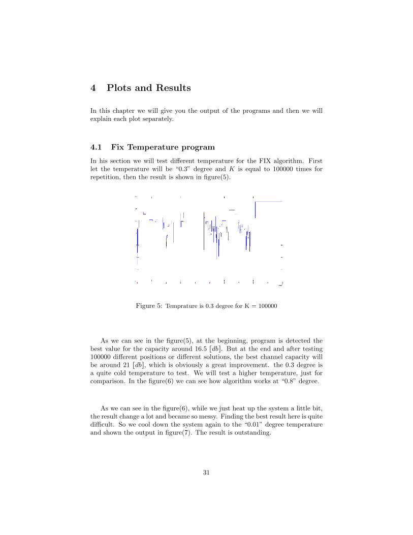
4.1 Fix Temperature program

In his section we will test different temperature for the FIX algorithm. Firstlet the temperature will be “0.3” degree and K is equal to 100000 times forrepetition, then the result is shown in figure(5).

Figure 5: Temprature is 0.3 degree for K = 100000

As we can see in the figure(5), at the beginning, program is detected thebest value for the capacity around 16.5 [db]. But at the end and after testing100000 different positions or different solutions, the best channel capacity willbe around 21 [db], which is obviously a great improvement. the 0.3 degree isa quite cold temperature to test. We will test a higher temperature, just forcomparison. In the figure(6) we can see how algorithm works at “0.8” degree.

As we can see in the figure(6), while we just heat up the system a little bit,the result change a lot and became so messy. Finding the best result here is quitedifficult. So we cool down the system again to the “0.01” degree temperatureand shown the output in figure(7). The result is outstanding.

31

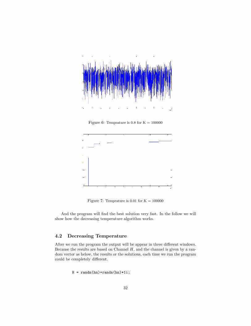
Figure 6: Temprature is 0.8 for K = 100000

Figure 7: Temprature is 0.01 for K = 100000

And the program will find the best solution very fast. In the follow we willshow how the decreasing temperature algorithm works.

4.2 Decreasing Temperature

After we run the program the output will be appear in three different windows.Because the results are based on Channel H, and the channel is given by a ran-dom vector as below, the results or the solutions, each time we run the programcould be completely different.

H = randn(hn)+randn(hn)*1i;

32

So the output for the Channel Capacity, Mean value for that and the tem-perature in one Sub-plot would be like figure(8):

Figure 8: Channel Capacity, Mean value for that and the temperature

To explain about the result in figure(8), first we draw each plot separately.

Figure 9: Channel Capacity for K = 1000 and q = 100

33

from the figure (9) we can see the algorithm will start by choosing the randomnumbers as the column and row. Then from the Boltzmann equation, we try toestimate best answer:

exp (Ci −Cmax

T) > [0,1), (38)

where Ci is the capacity of the channel for the current solution and Cmax isthe best solution. But here, because 100 is quite a big number compare to thedifference between the maximum and the current value of the channel capacity,so the exponential is almost one at the beginning, and so on all the solutionswill be accepted by algorithm. We can see here even if the current solution was10 and the maximum was 20:

exp (10 − 20

100) = 0.9048. (39)

Just because the temperature is so high, the result will be too close to 1and so almost all the selected random number in the area [0,1) will be less thanexponential and will be accepted.

But after a while, when the temperature rich to the 15 degree, then thepossibility of the acceptance is around 50 percent and the result will be improve:

exp (10 − 20

15) = 0.5134, (40)

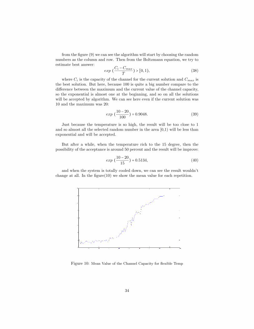
and when the system is totally cooled down, we can see the result wouldn’tchange at all. In the figure(10) we show the mean value for each repetition.

Figure 10: Mean Value of the Channel Capacity for flexible Temp

34

The mean value for channel capacity in the figure(10) shows that the resultimprove when the system cools down. The result started from around 15 [db]and after all process, finally when the system is cool enough, it reached to it’smaximum value around 21 [db].

And the best antenna positions are:

Rc = 53 6 74

Rr = 91 62 13

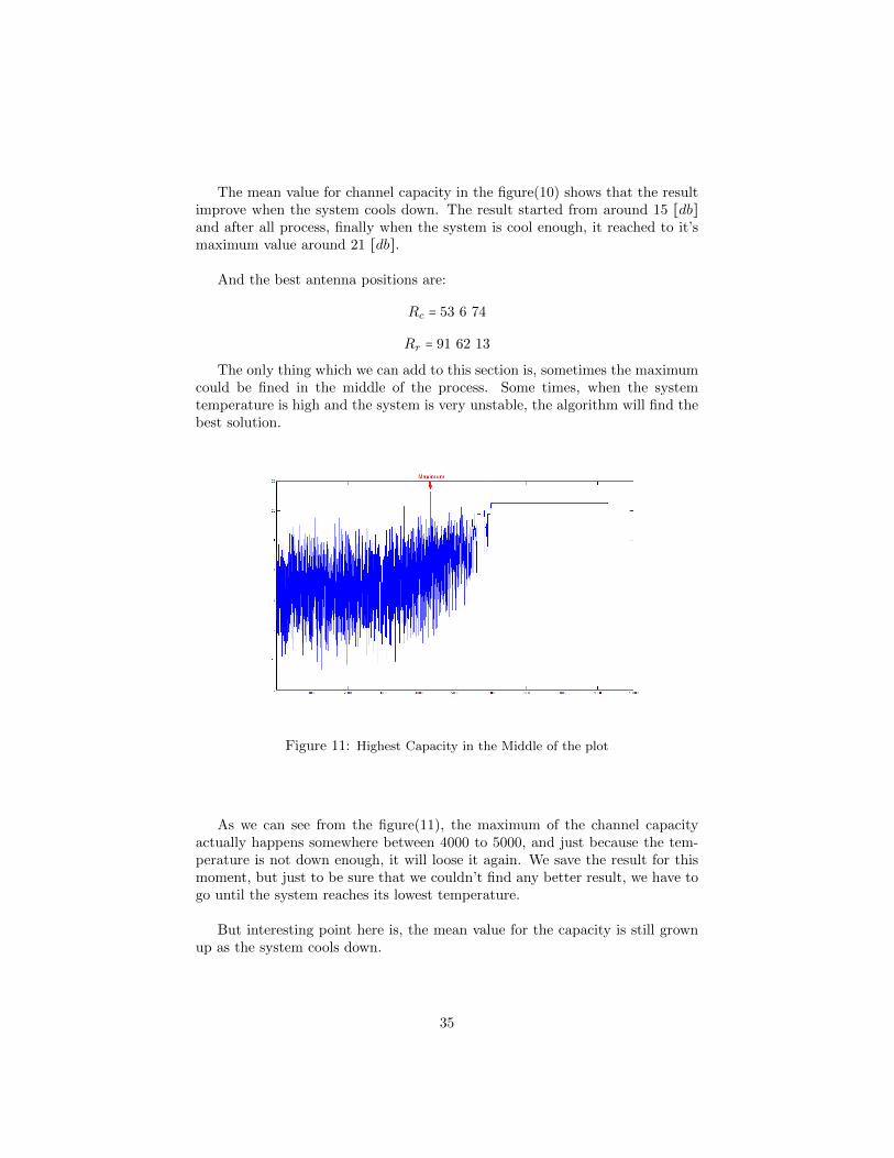
The only thing which we can add to this section is, sometimes the maximumcould be fined in the middle of the process. Some times, when the systemtemperature is high and the system is very unstable, the algorithm will find thebest solution.

Figure 11: Highest Capacity in the Middle of the plot

As we can see from the figure(11), the maximum of the channel capacityactually happens somewhere between 4000 to 5000, and just because the tem-perature is not down enough, it will loose it again. We save the result for thismoment, but just to be sure that we couldn’t find any better result, we have togo until the system reaches its lowest temperature.

But interesting point here is, the mean value for the capacity is still grownup as the system cools down.

35

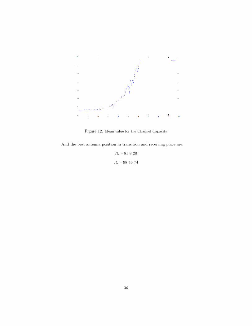
Figure 12: Mean value for the Channel Capacity

And the best antenna position in transition and receiving place are:

Rc = 81 8 20

Rr = 98 46 74

36

Conculusion

In general, we have lot’s of possible solutions for a specific problem. If solv-ing the problem takes a lot of time, there are different way to reach the answerfaster and easier. Here we choose the Annealing Simulation to find one of thebest solution. The best solution from this method, shouldn’t always be the bestpossible one, but it’s almost always is close enough to that, which we can countit as the best solution.

For this report, as we mention before, we had to find 3 position form 100,where the channel capacity is the highest. So, first we write a MATLAB codefor very basic situation, where the temperature were fix and the input/outputantenna positions were fix and we didn’t have that much freedom to select dif-ferent functionality.

Then by extending the basic program to the next level we add some func-tionality to the program, which help us to reach the better possible solution inthe less time. And finally we put every things in a GUI window.

37

5 References

References

[1] E Aarts and J Korst, Simulated Annealing and Boltzmann Ma-chines. Wiley, Chichester, UK, 1989.

[2] Van Laarhoven, Simulated annealing: theory and applications.Dordrecht Boston Norwell, MA, U.S.A, 1987.

[3] T Cover, Elements of information theory. Wiley, New York, 1991.

[4] John Proakis, Digital communications. McGraw-Hill, New York, 1995.

[5] David Brown, Managing Performance and Capacity. Prentice Hal,2011.

38

A MATLAB Programs

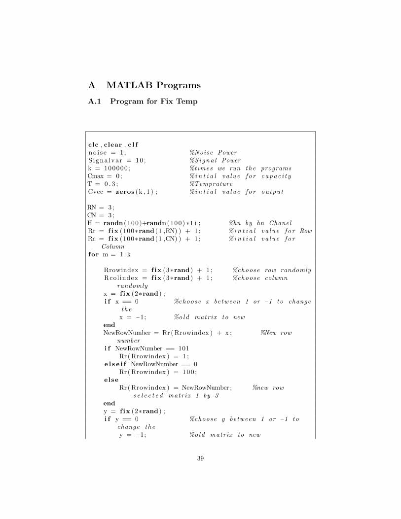
A.1 Program for Fix Temp

clc , clear , c l fno i s e = 1 ; %Noise PowerS igna lva r = 10 ; %S i g n a l Powerk = 100000; %times we run the programsCmax = 0 ; %i n t i a l v a l u e f o r c a p a c i t yT = 0 . 3 ; %TempratureCvec = zeros (k , 1 ) ; %i n t i a l v a l u e f o r output

RN = 3 ;CN = 3 ;H = randn (100)+randn (100) ∗1 i ; %hn by hn ChanelRr = f ix (100∗rand (1 ,RN) ) + 1 ; %i n t i a l v a l u e f o r RowRc = f ix (100∗rand (1 ,CN) ) + 1 ; %i n t i a l v a l u e f o r

Columnfor m = 1 : k

Rrowindex = f ix (3∗rand ) + 1 ; %choose row randomlyRcol index = f ix (3∗rand ) + 1 ; %choose column

randomlyx = f ix (2∗rand ) ;i f x == 0 %choose x between 1 or −1 to change

thex = −1; %o l d matrix to new

endNewRowNumber = Rr( Rrowindex ) + x ; %New row

numberi f NewRowNumber == 101

Rr( Rrowindex ) = 1 ;e l s e i f NewRowNumber == 0

Rr( Rrowindex ) = 100 ;else

Rr( Rrowindex ) = NewRowNumber ; %new rows e l e c t e d matrix 1 by 3

endy = f ix (2∗rand ) ;i f y == 0 %choose y between 1 or −1 to

change they = −1; %o l d matrix to new

39

endNewColNumber = Rc( Rcol index ) + y ; %new column

numberi f NewColNumber == 101

Rc( Rcol index ) = 1 ;e l s e i f NewColNumber == 0

Rc( Rcol index ) = 100 ;else

Rc( Rcol index ) = NewColNumber ;end %new column s e l e c t e d matrix

1 by 3

Hm= H(Rr , Rc) ; % random s e l e c t e d matrix fromthe H

Cm = log2 ( det ( ( eye (RN)+( S igna lva r / no i s e ) ∗(Hm∗Hm’ ) ) ) ) ;

%3 by 3 chane l Capacitance

i f Cm >= Cmax%t e s t i n g the new v a l u e o f c a p a c i t y wi th

the p e r i v o u s one%and i f i t ’ s g r e a t e r r e p l a c e i t !

BR = Rr ;BC = Rc ;Cmax = Cm;

e l s e i f exp ( (Cm−Cmax) /T) > rand ;BR = Rr ;BC = Rc ;Cmax = Cm;

end

Cvec (m) = Cmax;

enddisp ( ’The Best P o s i t i o n s f o r The Antenas : ’ ) , disp (BR) ;disp (BC) ;plot ( ( real ( Cvec ) ) )

40

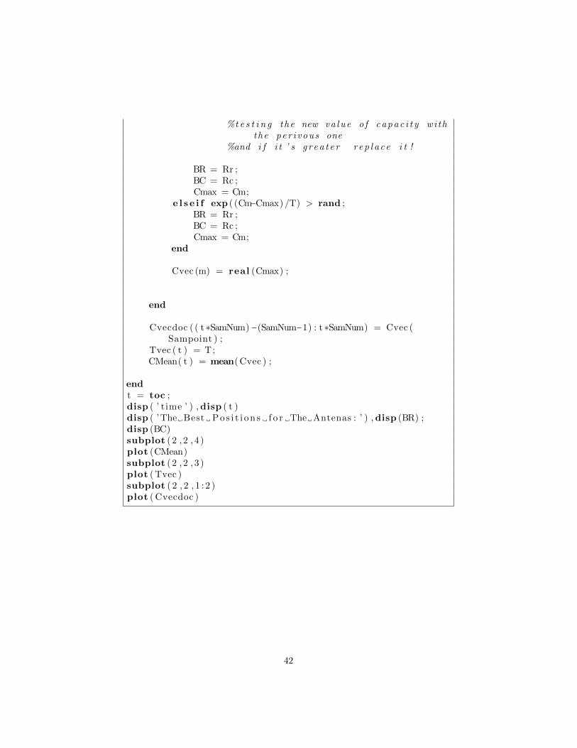
A.2 Program for Flexible Temp

t ic ;n o i s e = 1 ; %Noise PowerS igna lva r = 10 ; %S i g n a l Powerk = 1000 ; %times we run the

programsq = 100 ; %d i v i d e d Time l e n g t hCmax = 0 ; %i n t i a l v a l u e c a p a c i t yTstart = 100 ; Tstop = 0 . 0 1 ; %TempraturesT = Tstart ; %i n t i a l v a l u e f o r Ta = 10ˆ( log10 ( Tstop/ Tstart ) /q ) ; %Temprature c o e f f i c e n tCvec = zeros (k , 1 ) ; %i n t i a l v a l u e f o r

outputCMean = zeros (q , 1 ) ;Tvec = zeros (q , 1 ) ;SamNum = k /10 ;Sampoint = f ix ( linspace (1 , k ,SamNum) ) ; %Samling

i n t e r v a lCvecdoc = zeros (SamNum, 1 ) ;RN = 3 ;RC = 3 ;hn = 100 ;H = randn(hn)+randn(hn) ∗1 i ; %hn by hn ChanelRr = f ix (hn∗rand (1 ,RN) ) + 1 ; %i n t i a l Random RowRc = f ix (hn∗rand (1 ,RC) ) + 1 ; %i n t i a l Random Column

for t = 1 : qT = T∗a ;

for m = 1 : k

[ Rr , Rc ] = Randomize (Rr , Rc , hn) ;

Rr = NonEqualElements (Rr , hn ) ;Rc = NonEqualElements (Rc , hn) ;

Hm= H(Rr , Rc) ; % Random s e l e c t e d matrix H

Cm = log2 ( det ( ( eye (RN)+( S igna lva r / no i s e ) ∗(Hm∗Hm’ )) ) ) ;

% Chanel Capacitance

i f Cm > Cmax

41

%t e s t i n g the new v a l u e o f c a p a c i t y wi ththe p e r i v o u s one

%and i f i t ’ s g r e a t e r r e p l a c e i t !



end

Cvec (m) = real (Cmax) ;

end

Cvecdoc ( ( t ∗SamNum) −(SamNum−1) : t ∗SamNum) = Cvec (Sampoint ) ;

Tvec ( t ) = T;CMean( t ) = mean( Cvec ) ;

endt = toc ;disp ( ’ time ’ ) , disp ( t )disp ( ’The Best P o s i t i o n s f o r The Antenas : ’ ) , disp (BR) ;disp (BC)subplot ( 2 , 2 , 4 )plot (CMean)subplot ( 2 , 2 , 3 )plot ( Tvec )subplot ( 2 , 2 , 1 : 2 )plot ( Cvecdoc )

42

B Functions

B.1 Randomize function

function [ Rr , Rc ] = Randomize (Rr , Rc , hn)RR = length (Rr) ;RC = length (Rc) ;Rrowindex = f ix (RR∗rand ) + 1 ;Rcol index = f ix (RC∗rand ) + 1 ;x = f ix (2∗rand ) ;i f x == 0

x = −1;endNewRowNumber = Rr( Rrowindex ) + x ;i f NewRowNumber == hn+1

Rr( Rrowindex ) = 1 ;e l s e i f NewRowNumber == 0

Rr( Rrowindex ) = hn ;else

Rr( Rrowindex ) = NewRowNumber ;endy = f ix (2∗rand ) ;i f y == 0

y = −1;endNewColNumber = Rc( Rcol index ) + y ;i f NewColNumber == hn+1

Rc( Rcol index ) = 1 ;e l s e i f NewColNumber == 0

Rc( Rcol index ) = hn ;else

Rc( Rcol index ) = NewColNumber ;end

43

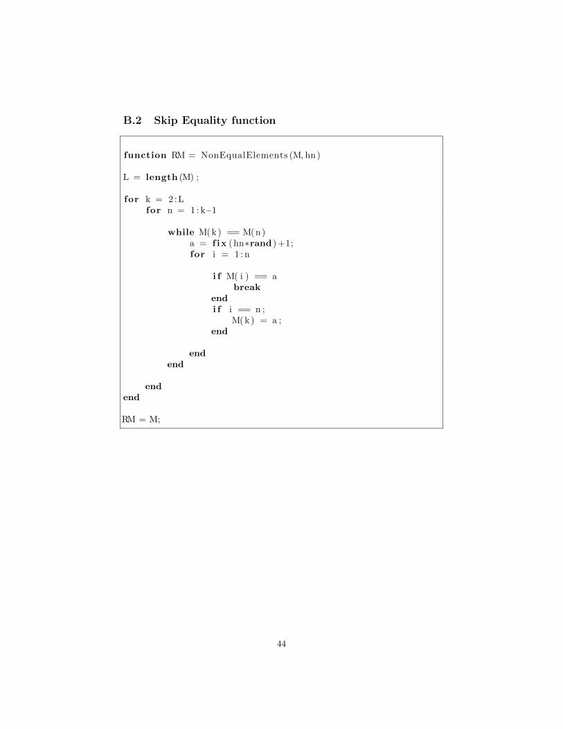
B.2 Skip Equality function

function RM = NonEqualElements (M, hn)

L = length (M) ;

for k = 2 :Lfor n = 1 : k−1

while M( k ) == M(n)a = f ix (hn∗rand ) +1;for i = 1 : n

i f M( i ) == abreak

endi f i == n ;

M( k ) = a ;end

endend

endend

RM = M;

44

C GUI codes

function varargout = GUIAnnealing ( vararg in )%GUIANNEALING M− f i l e f o r GUIAnnealing . f i g% GUIANNEALING, by i t s e l f , c r e a t e s a new

GUIANNEALING or r a i s e s the e x i s t i n g% s i n g l e t o n ∗ .%% H = GUIANNEALING r e t u r n s the handle to a new

GUIANNEALING or the handle to% the e x i s t i n g s i n g l e t o n ∗ .%% GUIANNEALING( ’ Property ’ , ’ Value ’ , . . . ) c r e a t e s a new

GUIANNEALING using the% given prop er t y v a l u e p a i r s . Unrecognized

p r o p e r t i e s are passed v i a% v ara rg in to GUIAnnealing OpeningFcn . This c a l l i n g

syntax produces a% warning when t h e r e i s an e x i s t i n g s i n g l e t o n ∗ .%% GUIANNEALING( ’CALLBACK’ ) and GUIANNEALING( ’

CALLBACK’ , hObject , . . . ) c a l l the% l o c a l f u n c t i o n named CALLBACK in GUIANNEALING.M

with the g iven input% arguments .%% ∗See GUI Options on GUIDE’ s Tools menu . Choose ”

GUI a l l o w s only one% i n s t a n c e to run ( s i n g l e t o n ) ” .%% See a l s o : GUIDE, GUIDATA, GUIHANDLES

% Edit the above t e x t to modify the response to h e l pGUIAnnealing

% Last Modif ied by GUIDE v2 .5 22−Nov−2012 16 :01 :15

% Begin i n i t i a l i z a t i o n code − DO NOT EDITg u i S i n g l e t o n = 1 ;g u i S t a t e = s t r u c t ( ’ gui Name ’ , mfilename , . . .

’ g u i S i n g l e t o n ’ , gu i S ing l e t on , . . .’ gui OpeningFcn ’ ,

@GUIAnnealing OpeningFcn , . . .

45

’ gui OutputFcn ’ ,@GUIAnnealing OutputFcn , . . .

’ gui LayoutFcn ’ , [ ] , . . .’ gu i Ca l lback ’ , [ ] ) ;

i f nargin && i s c h a r ( vararg in {1})g u i S t a t e . gu i Ca l lback = s t r 2 f u n c ( vararg in {1}) ;

end

i f nargout[ varargout {1 : nargout } ] = gui main fcn ( gu i S ta te ,

vara rg in { :} ) ;else

gui main fcn ( gu i S ta te , vara rg in { :} ) ;end% End i n i t i a l i z a t i o n code − DO NOT EDIT

% −−− Executes j u s t b e f o r e GUIAnnealing i s made v i s i b l e .function GUIAnnealing OpeningFcn ( hObject , eventdata ,

handles , vararg in )% This f u n c t i o n has no output args , see OutputFcn .% hObject handle to f i g u r e% eventda ta r e s e r v e d − to be d e f i n e d in a f u t u r e v e r s i o n

o f MATLAB% hand les s t r u c t u r e wi th hand les and user data ( see

GUIDATA)% v ara rg in unrecognized PropertyName/ PropertyValue

p a i r s from the% command l i n e ( see VARARGIN)

% Choose d e f a u l t command l i n e output f o r GUIAnnealinghandles . output = hObject ;

% Update hand les s t r u c t u r eguidata ( hObject , handles ) ;

% UIWAIT makes GUIAnnealing wai t f o r user response ( seeUIRESUME)

% u i w a i t ( hand les . f i g u r e 1 ) ;

% −−− Outputs from t h i s f u n c t i o n are re turned to thecommand l i n e .

function varargout = GUIAnnealing OutputFcn ( hObject ,eventdata , handles )

46

% varargout c e l l array f o r r e t u r n i n g output args ( seeVARARGOUT) ;

% hObject handle to f i g u r e% eventda ta r e s e r v e d − to be d e f i n e d in a f u t u r e v e r s i o n


GUIDATA)

% Get d e f a u l t command l i n e output from hand les s t r u c t u r evarargout {1} = handles . output ;

% −−− Executes on but ton p r e s s in PLOT.function PLOT Callback ( hObject , eventdata , handles )% hObject handle to PLOT ( see GCBO)% eventda ta r e s e r v e d − to be d e f i n e d in a f u t u r e v e r s i o n


GUIDATA)

function SP Callback ( hObject , eventdata , handles )% hObject handle to SP ( see GCBO)% eventda ta r e s e r v e d − to be d e f i n e d in a f u t u r e v e r s i o n


GUIDATA)

% Hints : g e t ( hObject , ’ S tr ing ’ ) r e t u r n s c o n t e n t s o f SP ast e x t

% s t r 2 d o u b l e ( g e t ( hObject , ’ S tr ing ’ ) ) r e t u r n sc o n t e n t s o f SP as a doub le

% −−− Executes during o b j e c t crea t ion , a f t e r s e t t i n g a l lp r o p e r t i e s .

function SP CreateFcn ( hObject , eventdata , handles )% hObject handle to SP ( see GCBO)% eventda ta r e s e r v e d − to be d e f i n e d in a f u t u r e v e r s i o n

o f MATLAB% hand les empty − hand les not c r e a t e d u n t i l a f t e r a l l

CreateFcns c a l l e d

% Hint : e d i t c o n t r o l s u s u a l l y have a whi te background onWindows .

47

% See ISPC and COMPUTER.i f i s p c && i s e q u a l ( get ( hObject , ’ BackgroundColor ’ ) , get (0 ,

’ de fau l tUicontro lBackgroundColor ’ ) )set ( hObject , ’ BackgroundColor ’ , ’ white ’ ) ;

end

function NP Callback ( hObject , eventdata , handles )% hObject handle to NP ( see GCBO)% eventda ta r e s e r v e d − to be d e f i n e d in a f u t u r e v e r s i o n


GUIDATA)

% Hints : g e t ( hObject , ’ S tr ing ’ ) r e t u r n s c o n t e n t s o f NP ast e x t

% s t r 2 d o u b l e ( g e t ( hObject , ’ S tr ing ’ ) ) r e t u r n sc o n t e n t s o f NP as a doub le


function NP CreateFcn ( hObject , eventdata , handles )% hObject handle to NP ( see GCBO)% eventda ta r e s e r v e d − to be d e f i n e d in a f u t u r e v e r s i o n






end

function FK Callback ( hObject , eventdata , handles )% hObject handle to FK ( see GCBO)% eventda ta r e s e r v e d − to be d e f i n e d in a f u t u r e v e r s i o n


GUIDATA)

48

% Hints : g e t ( hObject , ’ S tr ing ’ ) r e t u r n s c o n t e n t s o f FK ast e x t

% s t r 2 d o u b l e ( g e t ( hObject , ’ S tr ing ’ ) ) r e t u r n sc o n t e n t s o f FK as a doub le


function FK CreateFcn ( hObject , eventdata , handles )% hObject handle to FK ( see GCBO)% eventda ta r e s e r v e d − to be d e f i n e d in a f u t u r e v e r s i o n






end

function FT Callback ( hObject , eventdata , handles )% hObject handle to FT ( see GCBO)% eventda ta r e s e r v e d − to be d e f i n e d in a f u t u r e v e r s i o n


GUIDATA)

% Hints : g e t ( hObject , ’ S tr ing ’ ) r e t u r n s c o n t e n t s o f FT ast e x t

% s t r 2 d o u b l e ( g e t ( hObject , ’ S tr ing ’ ) ) r e t u r n sc o n t e n t s o f FT as a doub le


function FT CreateFcn ( hObject , eventdata , handles )% hObject handle to FT ( see GCBO)% eventda ta r e s e r v e d − to be d e f i n e d in a f u t u r e v e r s i o n

o f MATLAB

49

% hand les empty − hand les not c r e a t e d u n t i l a f t e r a l lCreateFcns c a l l e d




end

function Tstar t Ca l lback ( hObject , eventdata , handles )% hObject handle to Ts tar t ( see GCBO)% eventda ta r e s e r v e d − to be d e f i n e d in a f u t u r e v e r s i o n


GUIDATA)

% Hints : g e t ( hObject , ’ S tr ing ’ ) r e t u r n s c o n t e n t s o f Ts tar tas t e x t

% s t r 2 d o u b l e ( g e t ( hObject , ’ S tr ing ’ ) ) r e t u r n sc o n t e n t s o f Ts tar t as a doub le


function Tstart CreateFcn ( hObject , eventdata , handles )% hObject handle to Ts tar t ( see GCBO)% eventda ta r e s e r v e d − to be d e f i n e d in a f u t u r e v e r s i o n






end

function Tstop Cal lback ( hObject , eventdata , handles )

50

% hObject handle to Tstop ( see GCBO)% eventda ta r e s e r v e d − to be d e f i n e d in a f u t u r e v e r s i o n


GUIDATA)

% Hints : g e t ( hObject , ’ S tr ing ’ ) r e t u r n s c o n t e n t s o f Tstopas t e x t

% s t r 2 d o u b l e ( g e t ( hObject , ’ S tr ing ’ ) ) r e t u r n sc o n t e n t s o f Tstop as a doub le


function Tstop CreateFcn ( hObject , eventdata , handles )% hObject handle to Tstop ( see GCBO)% eventda ta r e s e r v e d − to be d e f i n e d in a f u t u r e v e r s i o n






end

function KC Callback ( hObject , eventdata , handles )% hObject handle to KC ( see GCBO)% eventda ta r e s e r v e d − to be d e f i n e d in a f u t u r e v e r s i o n


GUIDATA)

% Hints : g e t ( hObject , ’ S tr ing ’ ) r e t u r n s c o n t e n t s o f KC ast e x t

% s t r 2 d o u b l e ( g e t ( hObject , ’ S tr ing ’ ) ) r e t u r n sc o n t e n t s o f KC as a doub le


51

function KC CreateFcn ( hObject , eventdata , handles )% hObject handle to KC ( see GCBO)% eventda ta r e s e r v e d − to be d e f i n e d in a f u t u r e v e r s i o n






end

function Q Callback ( hObject , eventdata , handles )% hObject handle to Q ( see GCBO)% eventda ta r e s e r v e d − to be d e f i n e d in a f u t u r e v e r s i o n


GUIDATA)

% Hints : g e t ( hObject , ’ S tr ing ’ ) r e t u r n s c o n t e n t s o f Q ast e x t

% s t r 2 d o u b l e ( g e t ( hObject , ’ S tr ing ’ ) ) r e t u r n sc o n t e n t s o f Q as a doub le


function Q CreateFcn ( hObject , eventdata , handles )% hObject handle to Q ( see GCBO)% eventda ta r e s e r v e d − to be d e f i n e d in a f u t u r e v e r s i o n






end

52

% −−− Executes on s e l e c t i o n change in l i s t b o x 1 .function l i s t b o x 1 C a l l b a c k ( hObject , eventdata , handles )% hObject handle to l i s t b o x 1 ( see GCBO)% eventda ta r e s e r v e d − to be d e f i n e d in a f u t u r e v e r s i o n


GUIDATA)

% Hints : c o n t e n t s = c e l l s t r ( g e t ( hObject , ’ S tr ing ’ ) )r e t u r n s l i s t b o x 1 c o n t e n t s as c e l l array

% c o n t e n t s { g e t ( hObject , ’ Value ’ ) } r e t u r n s s e l e c t e ditem from l i s t b o x 1


function l i s tbox1 CreateFcn ( hObject , eventdata , handles )% hObject handle to l i s t b o x 1 ( see GCBO)% eventda ta r e s e r v e d − to be d e f i n e d in a f u t u r e v e r s i o n



% Hint : l i s t b o x c o n t r o l s u s u a l l y have a whi te backgroundon Windows .



end

function ed i t 10 Ca l l back ( hObject , eventdata , handles )% hObject handle to Ts tar t ( see GCBO)% eventda ta r e s e r v e d − to be d e f i n e d in a f u t u r e v e r s i o n


GUIDATA)

% Hints : g e t ( hObject , ’ S tr ing ’ ) r e t u r n s c o n t e n t s o f Ts tar tas t e x t

% s t r 2 d o u b l e ( g e t ( hObject , ’ S tr ing ’ ) ) r e t u r n sc o n t e n t s o f Ts tar t as a doub le

53


function ed i t10 CreateFcn ( hObject , eventdata , handles )% hObject handle to Ts tar t ( see GCBO)% eventda ta r e s e r v e d − to be d e f i n e d in a f u t u r e v e r s i o n






end

function ed i t 11 Ca l l back ( hObject , eventdata , handles )% hObject handle to Tstop ( see GCBO)% eventda ta r e s e r v e d − to be d e f i n e d in a f u t u r e v e r s i o n


GUIDATA)

% Hints : g e t ( hObject , ’ S tr ing ’ ) r e t u r n s c o n t e n t s o f Tstopas t e x t

% s t r 2 d o u b l e ( g e t ( hObject , ’ S tr ing ’ ) ) r e t u r n sc o n t e n t s o f Tstop as a doub le


function ed i t11 CreateFcn ( hObject , eventdata , handles )% hObject handle to Tstop ( see GCBO)% eventda ta r e s e r v e d − to be d e f i n e d in a f u t u r e v e r s i o n




% See ISPC and COMPUTER.

54

i f i s p c && i s e q u a l ( get ( hObject , ’ BackgroundColor ’ ) , get (0 ,’ de fau l tUicontro lBackgroundColor ’ ) )set ( hObject , ’ BackgroundColor ’ , ’ white ’ ) ;

end

function CK Callback ( hObject , eventdata , handles )% hObject handle to CK ( see GCBO)% eventda ta r e s e r v e d − to be d e f i n e d in a f u t u r e v e r s i o n


GUIDATA)

% Hints : g e t ( hObject , ’ S tr ing ’ ) r e t u r n s c o n t e n t s o f CK ast e x t

% s t r 2 d o u b l e ( g e t ( hObject , ’ S tr ing ’ ) ) r e t u r n sc o n t e n t s o f CK as a doub le


function CK CreateFcn ( hObject , eventdata , handles )% hObject handle to CK ( see GCBO)% eventda ta r e s e r v e d − to be d e f i n e d in a f u t u r e v e r s i o n






end

function ed i t 13 Ca l l back ( hObject , eventdata , handles )% hObject handle to Q ( see GCBO)% eventda ta r e s e r v e d − to be d e f i n e d in a f u t u r e v e r s i o n


GUIDATA)

55

% Hints : g e t ( hObject , ’ S tr ing ’ ) r e t u r n s c o n t e n t s o f Q ast e x t

% s t r 2 d o u b l e ( g e t ( hObject , ’ S tr ing ’ ) ) r e t u r n sc o n t e n t s o f Q as a doub le


function ed i t13 CreateFcn ( hObject , eventdata , handles )% hObject handle to Q ( see GCBO)% eventda ta r e s e r v e d − to be d e f i n e d in a f u t u r e v e r s i o n






end

function channe l Ca l lback ( hObject , eventdata , handles )% hObject handle to channel ( see GCBO)% eventda ta r e s e r v e d − to be d e f i n e d in a f u t u r e v e r s i o n


GUIDATA)

% Hints : g e t ( hObject , ’ S tr ing ’ ) r e t u r n s c o n t e n t s o fchannel as t e x t

% s t r 2 d o u b l e ( g e t ( hObject , ’ S tr ing ’ ) ) r e t u r n sc o n t e n t s o f channel as a doub le


function channel CreateFcn ( hObject , eventdata , handles )% hObject handle to channel ( see GCBO)% eventda ta r e s e r v e d − to be d e f i n e d in a f u t u r e v e r s i o n



56




end

function CNN Callback ( hObject , eventdata , handles )% hObject handle to CNN ( see GCBO)% eventda ta r e s e r v e d − to be d e f i n e d in a f u t u r e v e r s i o n


GUIDATA)

% Hints : g e t ( hObject , ’ S tr ing ’ ) r e t u r n s c o n t e n t s o f CNN ast e x t

% s t r 2 d o u b l e ( g e t ( hObject , ’ S tr ing ’ ) ) r e t u r n sc o n t e n t s o f CNN as a doub le


function CNN CreateFcn ( hObject , eventdata , handles )% hObject handle to CNN ( see GCBO)% eventda ta r e s e r v e d − to be d e f i n e d in a f u t u r e v e r s i o n






end

function RNN Callback ( hObject , eventdata , handles )% hObject handle to RNN ( see GCBO)

57

% eventda ta r e s e r v e d − to be d e f i n e d in a f u t u r e v e r s i o no f MATLAB

% hand les s t r u c t u r e wi th hand les and user data ( seeGUIDATA)

% Hints : g e t ( hObject , ’ S tr ing ’ ) r e t u r n s c o n t e n t s o f RNN ast e x t

% s t r 2 d o u b l e ( g e t ( hObject , ’ S tr ing ’ ) ) r e t u r n sc o n t e n t s o f RNN as a doub le


function RNN CreateFcn ( hObject , eventdata , handles )% hObject handle to RNN ( see GCBO)% eventda ta r e s e r v e d − to be d e f i n e d in a f u t u r e v e r s i o n






end

%−−−−−−−−−−−−−−−−−−−−−−−−−−−−−−−−−−−−−−−−−−−−−−−−−−−−−−−−−−−−−−−−−−−−

function uipanel4 ButtonDownFcn ( hObject , eventdata ,handles )

% hObject handle to u ipa ne l4 ( see GCBO)% eventda ta r e s e r v e d − to be d e f i n e d in a f u t u r e v e r s i o n


GUIDATA)

% −−− Executes on but ton p r e s s in pushbut ton1 .function pushbutton1 Cal lback ( hObject , eventdata , handles

)% hObject handle to pushbut ton1 ( see GCBO)

58

% eventda ta r e s e r v e d − to be d e f i n e d in a f u t u r e v e r s i o no f MATLAB

% hand les s t r u c t u r e wi th hand les and user data ( seeGUIDATA)

np = get ( handles .NP, ’ s t r i n g ’ ) ;no i s e = str2num(np) ; %Noise Power

sp = get ( handles . SP , ’ s t r i n g ’ ) ;S i gna lva r = str2num( sp ) ; %S i g n a l Power

fk = get ( handles .FK, ’ s t r i n g ’ ) ;k = str2num( fk ) ; %times we run the

programs

Cmax = 0 ; %i n t i a l v a l u e f o rt e s t i n g the maximum c a p a c i t y o f the chane l

rn = get ( handles .RNN, ’ s t r i n g ’ ) ;RN = str2num( rn ) ;

cn = get ( handles .CNN, ’ s t r i n g ’ ) ;CN = str2num( cn ) ;

f t = get ( handles .FT, ’ s t r i n g ’ ) ;T = str2num( f t ) ; %Temprature

Cvec = zeros (k , 1 ) ; %i n t i a l v a l u e f o routput

chann = get ( handles . channel , ’ s t r i n g ’ ) ;H = str2num( chann ) ; %100 by 100 Chanelhn = length (H) ;

Rr = f ix (hn∗rand (1 ,RN) ) + 1 ; %i n t i a l v a l u e f o rRandom Row

Rc = f ix (hn∗rand (1 ,CN) ) + 1 ; %i n t i a l v a l u e f o rRandom Column

%%for m = 1 : k


59


Hm= H(Rr , Rc) ;Cm = log2 ( det ( ( eye (RN)+( S igna lva r / no i s e ) ∗(Hm∗Hm’ ) ) ) ) ;

%3 by 3 chane l Capacitance

i f Cm >= Cmax %t e s t i n g the new v a l u e o fc a p a c i t y wi th the p e r i v o u s one

BR = Rr ; %and i f i t ’ s g r e a t e rr e p l a c e i t !

BC = Rc ;Cmax = Cm;


end

Cvec (m) = Cmax;

end%%

global Cvec1 ;Cvec1 = Cvec ;global Cvec1 ;global PS ;PS = 0 ;global PS ;clc

disp ( ’The Best P o s i t i o n s f o r The Antenas : ’ ) , disp (BR) ;disp (BC) ;h1 = subplot ( 1 , 1 , 1 , ’ Parent ’ , handles . axe s pane l ) ;plot ( h1 , real ( Cvec ) ) ;l e g = legend ( ’ Cost Function ’ , 3 ) ;

% −−− Executes on but ton p r e s s in pushbut ton2 .

60

function pushbutton2 Cal lback ( hObject , eventdata , handles)

% hObject handle to pushbut ton2 ( see GCBO)% eventda ta r e s e r v e d − to be d e f i n e d in a f u t u r e v e r s i o n


GUIDATA)

t ic ;

np = get ( handles .NP, ’ s t r i n g ’ ) ;no i s e = str2num(np) ; %Noise Power

sp = get ( handles . SP , ’ s t r i n g ’ ) ;S i gna lva r = str2num( sp ) ; %S i g n a l Power

ck = get ( handles .CK, ’ s t r i n g ’ ) ;k = str2num( ck ) ; %times we run the

programs

q = get ( handles .Q, ’ s t r i n g ’ ) ;q = str2num( q ) ; %d i v i d e d Time

l e n g t h

Tvec = zeros (q , 1 ) ;

rn = get ( handles .RNN, ’ s t r i n g ’ ) ;RN = str2num( rn ) ;

cn = get ( handles .CNN, ’ s t r i n g ’ ) ;CN = str2num( cn ) ;

Cmax = 0 ; %i n t i a l v a l u e f o rt e s t i n g the maximum c a p a c i t y o f the chane l

TS = get ( handles . Tstart , ’ s t r i n g ’ ) ;Tstart = str2num(TS) ;

TST = get ( handles . Tstop , ’ s t r i n g ’ ) ;Tstop = str2num(TST) ; %Tempratures

T = Tstart ; %i n t i a l v a l u e f o r T togo to the loop

a = 10ˆ( log10 ( Tstop/ Tstart ) /q ) ; %Temprature Decresmentc o e f f i c e n t

61

Cvec = zeros (k , 1 ) ; %i n t i a l v a l u e f o routput

CMAX = zeros (q , 1 ) ;Cbest = 0 ;

chann = get ( handles . channel , ’ s t r i n g ’ ) ;H = str2num( chann ) ; %100 by 100 Chanelhn = length (H) ;

SamNum = k /10 ;Sampoint = f ix ( linspace (1 , k ,SamNum) ) ; %Samling

i n t e r v a lCvecdoc = zeros (SamNum, 1 ) ;

Rr = f ix (hn∗rand (1 ,RN) ) + 1 ; %i n t i a l v a l u e f o rRandom Row

Rc = f ix (hn∗rand (1 ,CN) ) + 1 ; %i n t i a l v a l u e f o rRandom Column

for t = 1 : q

T = T∗a ;

for m = 1 : k



Hm= H(Rr , Rc) ;

% random s e l e c t e d matrixfrom the H(100 by 100)

Cm = log2 ( det ( ( eye (RN)+( S igna lva r / no i s e ) ∗(Hm∗Hm’ )) ) ) ;

% chane l Capacitance

i f Cm > Cmax %t e s t i n g the new v a l u eo f c a p a c i t y wi th the p e r i v o u s one

BR = Rr ; %and i f i t ’ s g r e a t e rr e p l a c e i t !

BC = Rc ;

62

Cmax = Cm;e l s e i f exp ( (Cm−Cmax) /T) > rand ;


end

Cvec (m) = real (Cmax) ;

end

Cvecdoc ( ( t ∗SamNum) −(SamNum−1) : t ∗SamNum) = Cvec (Sampoint ) ;

Cmaximum = max( Cvec ) ;Cvecdoc ( ( t ∗SamNum) −(SamNum−1) )= Cbest ;i f Cmaximum > Cbest ;

Cbest = Cmaximum;Cvecdoc ( ( t ∗SamNum) −(SamNum−1) )= Cbest ;

end

Tvec ( t ) = T;CMAX( t ) = mean( Cvec ) ;

end

global CMAX1;CMAX1 = CMAX;global CMAX1;

global Cvecdoc1 ;Cvecdoc1 = Cvecdoc ;global Cvecdoc1 ;

global Tvec1 ;Tvec1 = Tvec ;global Tvec1 ;

global PS ;PS = 1 ;global PS ;clc

t = toc ;

disp ( ’ time ’ ) , disp ( t )

63

disp ( ’The Best P o s i t i o n s f o r The Antenas : ’ ) , disp (BR) ;disp (BC)

h12 = subplot ( 2 , 2 , 1 : 2 , ’ Parent ’ , handles . axe s pane l ) ;plot ( h12 , Cvecdoc , ’b ’ ) ;t i t l e ( ’ Cost Function ’ , ’ Color ’ , ’w ’ ) ;

h3 = subplot ( 2 , 2 , 3 , ’ Parent ’ , handles . axe s pane l ) ;plot ( h3 ,CMAX) ;t i t l e ( ’Mean o f the Cost Function ’ , ’ Color ’ , ’w ’ ) ;

h4 = subplot ( 2 , 2 , 4 , ’ Parent ’ , handles . axe s pane l ) ;plot ( h4 , Tvec , ’ r ’ ) ;t i t l e ( ’ Temperature ’ , ’ Color ’ , ’w ’ ) ;

% −−− Executes on but ton p r e s s in t o g g l e b u t t o n 3 .function togg l ebut ton3 Ca l lback ( hObject , eventdata ,

handles )% hObject handle to t o g g l e b u t t o n 3 ( see GCBO)% eventda ta r e s e r v e d − to be d e f i n e d in a f u t u r e v e r s i o n


GUIDATA)% Hint : g e t ( hObject , ’ Value ’ ) r e t u r n s t o g g l e s t a t e o f

t o g g l e b u t t o n 3

global PS ;

i f PS == 1 ;global Cvecdoc1 ;global CMAX1;global Tvec1 ;f igure (1 )h = subplot ( 2 , 2 , 1 : 2 ) ; plot (h , Cvecdoc1 , ’b ’ ) ; t i t l e ( ’

Cost Function ’ ) ;h = subplot ( 2 , 2 , 3 ) ; plot (h ,CMAX1) ; t i t l e ( ’Mean o f Cost

Function ’ ) ;h = subplot ( 2 , 2 , 4 ) ; plot (h , Tvec1 , ’ r ’ ) ; t i t l e ( ’

Temperature ’ ) ;else

global Cvec1 ;f igure (1 )plot ( real ( Cvec1 ) ) ;l e g = legend ( ’ Cost Function ’ , 3 ) ;

end

64

SE-391 82 Kalmar / SE-351 95 Växjö Tel +46 (0)772-28 80 00 [email protected] Lnu.se/dfm

simulated annealing - diva portallnu.diva-portal.org/smash/get/diva2:608429/fulltext01.pdf ·...

Documents