Some Course Notes

SIGNAL S & SYSTEMS

Part I: Introduction to signals and systems

Signals are detectable quantities used to convey information about time-varying physical phenomena.

Common examples of signals are human speech, temperature, pressure, and stock prices. Electrical

signals, normally expressed in the form of voltage or current waveforms, are some of the easiest signals to

generate and process.

Mathematically, signals are modeled as functions of one or more independent variables. Examples of

independent variables used to represent signals are time, frequency, or spatial coordinates.

Figure 1.1 illustrates some common signals and systems encountered in different fields of engineering,

with the physical systems represented in the left-hand column and the associated signals included in the

right-hand column.

Fig. 1.1. Examples of signals and systems. (a) An electrical circuit; (c) an audio recording system; (e) a

digital camera; and (g) a digital thermometer. Plots (b), (d), (f ), and (h) are output signals generated,

respectively, by the systems shown in (a), (c), (e), and (g).

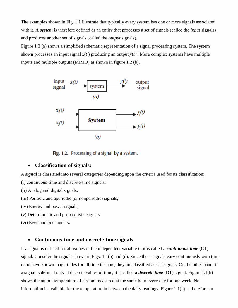
The examples shown in Fig. 1.1 illustrate that typically every system has one or more signals associated

with it. A system is therefore defined as an entity that processes a set of signals (called the input signals)

and produces another set of signals (called the output signals).

Figure 1.2 (a) shows a simplified schematic representation of a signal processing system. The system

shown processes an input signal x(t ) producing an output y(t ). More complex systems have multiple

inputs and multiple outputs (MIMO) as shown in figure 1.2 (b).

Classification of signals:

A signal is classified into several categories depending upon the criteria used for its classification:

(i) continuous-time and discrete-time signals;

(ii) Analog and digital signals;

(iii) Periodic and aperiodic (or nonperiodic) signals;

(iv) Energy and power signals;

(v) Deterministic and probabilistic signals;

(vi) Even and odd signals.

Continuous-time and discrete-time signals

If a signal is defined for all values of the independent variable t , it is called a continuous-time (CT)

signal. Consider the signals shown in Figs. 1.1(b) and (d). Since these signals vary continuously with time

t and have known magnitudes for all time instants, they are classified as CT signals. On the other hand, if

a signal is defined only at discrete values of time, it is called a discrete-time (DT) signal. Figure 1.1(h)

shows the output temperature of a room measured at the same hour every day for one week. No

information is available for the temperature in between the daily readings. Figure 1.1(h) is therefore an

example of a DT signal. In our notation, a CT signal is denoted by x(t ) with regular parenthesis, and a DT

signal is denoted with square parenthesis as follows:

x[nT ], n = 0, ±1, ±2, ±3, . . . ,

where T denotes the time interval between two consecutive samples. In the example of Fig. 1.1(h), the

value of T is one day.

Elementary signals

In this section, we define some elementary functions that will be used frequently to represent more

complicated signals. Representing signals in terms of the elementary functions simplifies the analysis and

design of linear systems.

1. Unit step function

The CT unit step function u(t ) is defined as follows:

The waveforms for the unit step functions u(t ) is shown in Fig.1.3. It is observed from Fig.1.3 that the CT

unit step function u(t ) is piecewise continuous with a discontinuity at t = 0. In other words, the rate of

change in u(t ) is infinite at t = 0.

Fig. 1.3: The waveforms for the unit step functions u(t ).

2. CT unit impulse function

The unit impulse function δ(t ), also known as the delta function, is defined as follows:

It is shown in Fig.1.6.

Fig.1.6: The unit impulse function.

The unit impulse may be visualized as a very short duration pulse of unit area. This may be expressed

mathematically as

To illustrate how the impulse function affects other functions, let us evaluate the integral

where Since , , except at t = t0 , Thus,

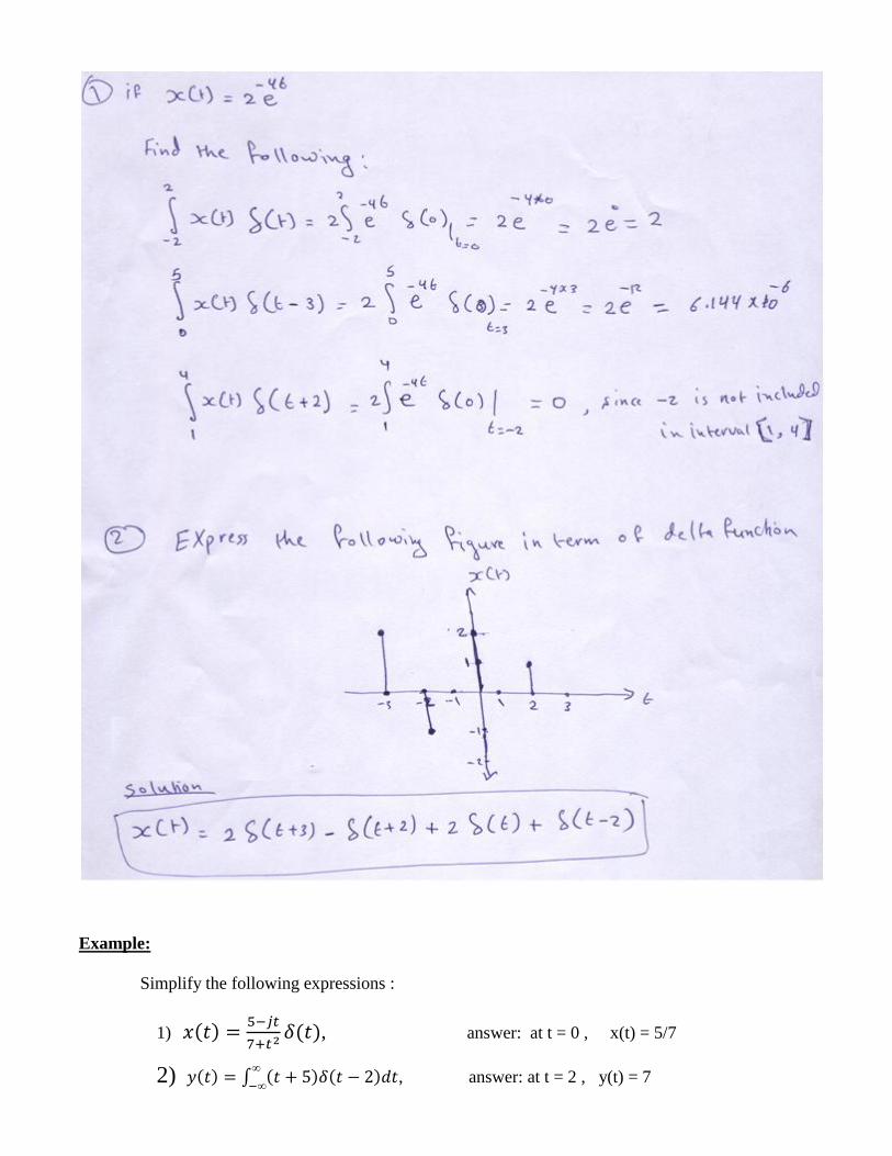
Example:

Simplify the following expressions :

1)

, answer: at t = 0 , x(t) = 5/7

2)

, answer: at t = 2 , y(t) = 7

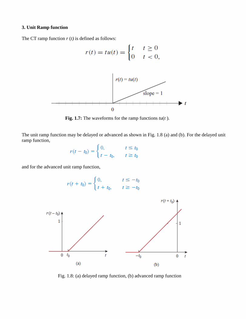
3. Unit Ramp function

The CT ramp function r (t) is defined as follows:

Fig. 1.7: The waveforms for the ramp functions tu(t ).

The unit ramp function may be delayed or advanced as shown in Fig. 1.8 (a) and (b). For the delayed unit

ramp function,

and for the advanced unit ramp function,

Fig. 1.8: (a) delayed ramp function, (b) advanced ramp function

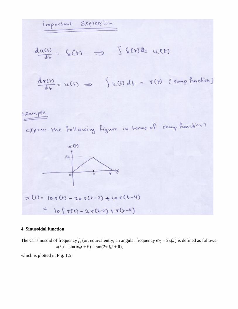
4. Sinusoidal function

The CT sinusoid of frequency fo (or, equivalently, an angular frequency ω0 = 2πfo ) is defined as follows:

x(t ) = sin(ω0t + θ) = sin(2π fot + θ),

which is plotted in Fig. 1.5

Fig. 1.9: The waveforms for CT sinusoidal functions.

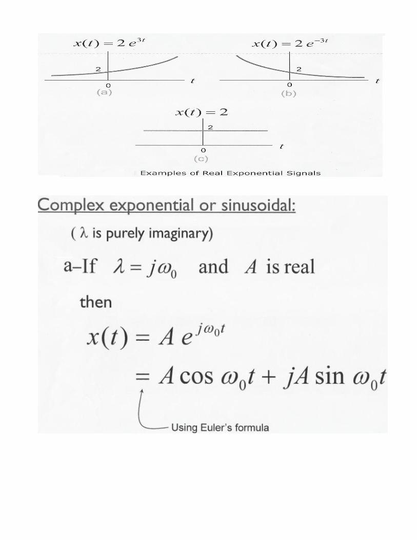
5. CT exponential function

A CT exponential function in general is represented by:

Periodic and aperiodic signals:

A CT signal x(t ) is said to be periodic if it satisfies the following property:

x(t ) = x(t + T0), at all time t and for some positive constant T0.

Where T0 is referred to as the fundamental period of x(t ).

A signal that is not periodic is called an aperiodic or non-periodic signal. Figure 1.11 shows examples of

both periodic and aperiodic signals. The reciprocal of the fundamental period of a signal is called the fun-

damental frequency. Mathematically, the fundamental frequency is expressed as follows

f0 =1/T0, for CT signals,

where T0 is the fundamental period of the CT signal. The frequency of a signal provides useful

information regarding how fast the signal changes its amplitude. The unit of frequency is cycles per

second (c/s) or hertz (Hz). Sometimes, we also use radians per second as a unit of frequency. Since there

are 2π radians (or 360◦) in one cycle, a frequency of f0 hertz is equivalent to 2π f0 radians per second. If

radians per second is used as a unit of frequency, the frequency is referred to as the angular frequency and

is given by

ω0 = 2π/T0

A familiar example of a periodic signal is a sinusoidal function represented mathematically by the

following expression:

x(t ) = A sin(ω0t + θ).

The sinusoidal signal x(t ) has a fundamental period T0 = 2π/ω0 as we prove next. Substituting t by t + T0 in

the sinusoidal function, yields x(t + T0) = A sin(ω0t + ω0T0 + θ).

Since x(t ) = A sin(ω0t + θ) = A sin(ω0t + 2kπ + θ), for k = 0,±1,±2, . . . ,

the above two expressions are equal iff ω0T0 = 2kπ. Selecting k = 1, the fundamental period is given by

T0 = 2π/ω0.

Fig. 1.11. Examples of periodic ((a), and (c), and aperiodic ((b) and (d) signals.

Examples

(i) CT sine wave: x1(t ) = sin(4πt ) is a periodic signal with period T1 = 2π/4π = 1/2;

(ii) CT cosine wave: x2(t ) = cos(3πt ) is a periodic signal with period T2 = 2π/3π = 2/3;

(iii) CT tangent wave: x3(t ) = tan(10t ) is a periodic signal with period T3 = π/10;

(iv) CT complex exponential: x4(t) = ej(2t+7)

is a periodic signal with period T4 = 2π/2 = π;

(v) CT sine wave of limited duration:

, is an aperiodic signal;

(vi) CT linear relationship: x6(t) = 2t + 5 is an aperiodic signal;

(vii) CT real exponential: x7(t) = e−2t

is an aperiodic signal.

Proposition : A signal g(t) that is a linear combination of two periodic signals, x1(t) with fundamental

period T1 and x2(t) with fundamental period T2 as follows:

g(t) = ax1(t ) + bx2(t ) is periodic iff

(rational number)

The fundamental period of g(t) is given by nT1 = mT2 provided that the values of m and n are chosen such

that the greatest common divisor (gcd) between m and n is 1 (i.e rational number).

Example

Determine if the following signals are periodic. If yes, determine the fundamental period.

(i) g1(t ) = 3 sin(4πt ) + 7 cos(3πt );

(ii) g2(t ) = 3 sin(4πt ) + 7 cos(10t ).

Solution

(i) In Example (i), we saw that the sinusoidal signals sin(4πt ) and cos(3πt ) are both periodic

signals with fundamental periods 1/2 and 2/3, respectively. Calculating the ratio of the two

fundamental periods yields:

which is a rational number. Hence, the linear combination g1(t ) is a periodic signal.

(ii) In Example (ii) , we saw that sin(4πt ) and 7cos(10t ) are both periodic signals with

fundamental periods 1/2 and π/5, respectively. Calculating the ratio of the two fundamental

periods yields:

which is not a rational number. Hence, the linear combination g2(t ) is not a periodic signal.

Deterministic and Random Signals:

Deterministic signals are those signals whose values are completely specified for any given time. Thus, a

deterministic signal can be modeled by a known function of time. Random signals are those signals that

take random values at any given time and must be characterized statistically. Random signals will not be

discussed in this text.

Deterministic signals can generally be expressed in a mathematical or graphical form. Some examples of

deterministic signals are as follows:

(1) CT sinusoidal signal: x1(t ) = 5 sin(20πt + 6);

(2) CT exponentially decaying sinusoidal signal: x2(t ) = 2e−t sin(7t ).

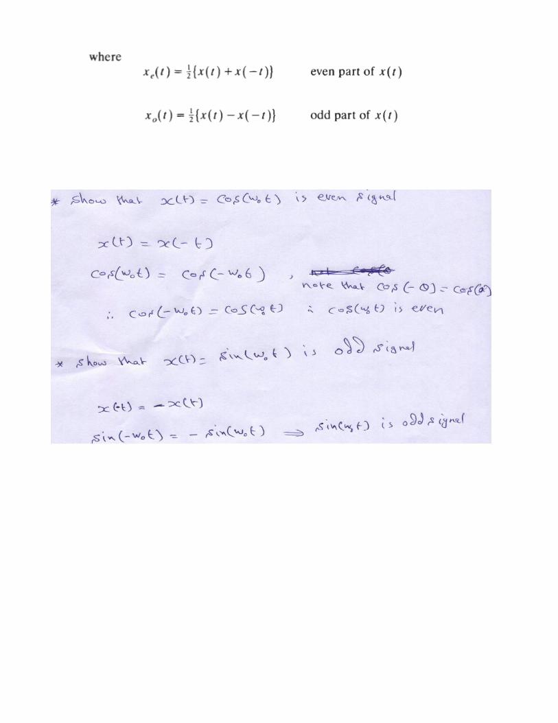
Even and Odd Signals:

A signal x ( t ) is referred to as an even signal if

x ( - t ) = x (t )

A signal x ( t ) is referred to as an odd signal if

x ( - t ) = - x ( t )

Examples of even and odd signals are shown in the following Figures:

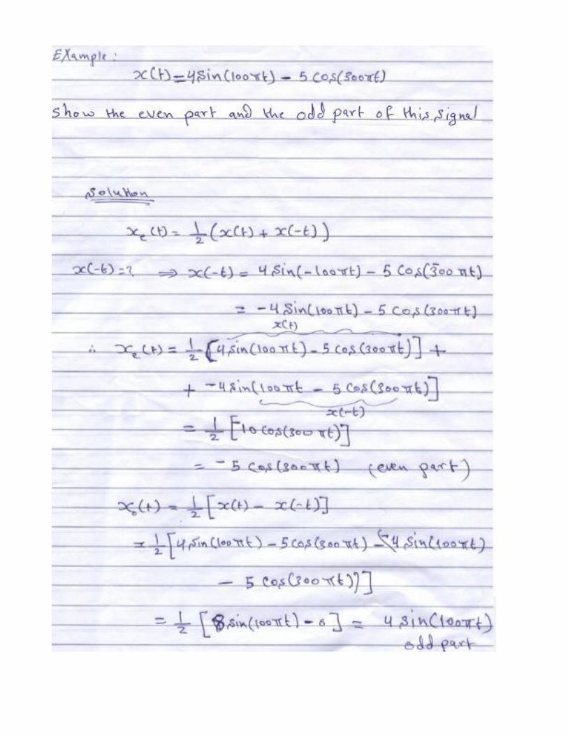
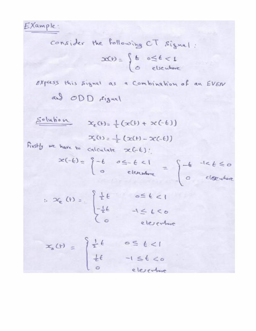
Any signal x(t) or x[n] can be expressed as a sum of two signals, one of which is even and one of which is

odd. That is,