Shift -Share Analysis: •

A Modified Approach

By Judith Z. Kalbacher*

INTRODUCTION

Traditionally, shift-share analysis has been used to describe regional growth or decline of a selected eco-nomic variable such as employment or income. The technique was appar-ently first applied by Daniel Creamer in 1942 (7, pp. 85-104),1 but it received little attention until Perloff, Dunn, Lampard, and Muth used shift share in a major work in regional analysis (13). Lowell D. Ashby, by introducing the technique to Govern-ment research, is credited for recogni-tion and popularity of the method as a tool for regional analysis.2

More recently, as analysts have turned from using descriptive regional statistics to models with predictive capabilities, several have criticized shift share. The pros and cons have been argued elsewhere and will not be presented here (3, pp. 423-425; 5, pp. 1-18; 6, p. 121; 8, pp. 115-120;

*The author is a geographer in the Economic Development Division, ESCS. Special recognition is given to Clark Edwards and Robert Coltrane, who proposed this work on relative shift-share analysis and provided guidance, critical review, and encour-agement. Appreciation is extended to Lon C. Cesal for work on various aspects of this article, and to Calvin L. Beale, the author's supervisor, for support and encouragement. Credit is also due to Vera J. Banks and Min-daugas F. Petrulis for their construc-tive review and to Suprina M. Wilson for her assistance in preparing the article.

' Italicized numbers in parentheses refer to items in References at the end of this article.

Ashby's major contributions using shift share are (1, pp. 13-20; 2).

This modified version of shift-share analy-sis presents components of regional eco-nomic growth in percentage terms. The version includes a comparative measure of industrial composition not present in traditional shift share. Key components of the modified approach are also shown in graph form to simplify the analysis of regional growth characteristics and the effects of change.

Keywords:

Shift-share analysis Regional economic growth

Components of regional economic growth Industry mix

Regional share

10, pp. 577-581). However, in work-ing with shift share, I have found that problems associated with using the technique often stem more from improper interpretation of results than from the methodology itself. When used descriptively to measure economic structure and change in a region against some norm, shift share is both useful and viable.

In this article, I use a different approach to the methodology. Tra-ditionally, results are presented as absolute numbers, which makes direct comparisons between regions and time periods difficult. In this modified approach, results are expressed as percentages to make interregional and intertemporal com-parisons easier.3 As another depar-ture, a comparative measure of industrial composition, not present in traditional shift share, is included.

3 L. H. Klaassen and J. H. P. Paelinck also use a relative form of shift-share analysis in (11, pp. 256-261). Other variations of the methodology in- clude: (4, pp. 59-68; 9, pp. 3-8; 12, pp. 283-292; 14, pp. 29-38).

•

COMPONENTS OF REGIONAL ECONOMIC

GROWTH

Both traditional and modified ver-sions of shift-share analysis divide regional economic growth into three components: standard growth, indus-try mix, and regional share. In the traditional version, an overall growth measure, the standard growth com-ponent, represents the norm against which a region's actual growth pat-terns are evaluated. Standard growth shows what growth would have been if change had occurred at the average rate of expansion in the designated reference economy.4 The amount by which actual growth is above or below this norm represents differen-tial regional growth, also termed net relative change.

Net relative change measures the shift of economic activity into or out of a region during a specified period. This shift is traceable either to the region's industrial mix or to the industries' growth performance local-ly compared with that of their coun-terparts in the reference economy (regional share).5

Because a region rarely produces specific goods and services in the same proportions as the reference economy, the region will experience more or less economic growth

4 Frequently, national growth pat-terns are selected as the standard for comparison. However, other refer-ence economies may be chosen, depending on the user's preference.

'The term locally refers to a char-acteristic of the particular economy being studied as opposed to the larger reference economy.

12 AGRICULTURAL ECONOMICS RESEARCH/VOL. 31, NO. 1, JANUARY 1979

•

depending on the industrial specialization. The industry mix component indicates whether local activity is con-centrated in sectors which, compared with the reference economy, grew faster or slower. Industry mix enables evaluation of the local economy's industrial composition. Regions with a relatively large positive industry mix component have a preponderance of fast-growth indus-tries. Such regions tend to have a higher propensity for long term growth than do regions with slower growing industries.

Growth attributed to the regional share component is a residual after standard trends and industry mix are allowed for. The regional share shows how the various industrial sectors grow in one region or another because of local economic forces. Growth performance of each industry in each region can be assessed by comparison with those of the reference economy. Here, regions in which industries are expanding more rapidly than their counterparts elsewhere are more likely to attract addi-tional economic activity.

As in traditional shift share, the modified version uses characteristics of a selected economy as a norm for com-parisons and accounts for differences between actual and standard growth in terms of industry mix and regional share. The approaches differ in two respects—the modi-fied version is expressed in percentages, and it includes a comparative measure of industrial composition. Although terms common to both versions have similar interpretations, standard growth and industry mix are defined differently. These differences and similarities are further clarified below.

THE METHODOLOGIES'

Traditional and this modified version of shift-share analysis may be described algebraically (fig. 1). Both versions require the same data; in this study, employ-ment data for nonmetropolitan counties of nine southern States were used (table 1). These nonmetro

For all data except when expressed in thousands, multiply numbers by 100 for exact correlation with data in tables.

counties serve as the designated reference economy, and nonmetro counties with predominantly black populations (50 percent or more) represent the study area.

Net Relative Change

The first step in applying shift-share analysis to em-ployment change in the predominantly black counties is to determine net relative change—the difference between actual and "standard" growth. In the traditional version, standard growth for each industry of the local region is calculated from aggregate growth in the reference region. In the modified version, specific industry growth rates for the reference region are used instead of the aggregate rate. Each industries' growth is weighted by that indus-try's importance in the reference region. This weighting introduces industry detail from the reference region into the modified shift share that is not used in the tradition-al analysis. We thus enhance interpretation of standard growth, but must redefine the industry mix component to incorporate this change.

The following equation expresses net relative change for the ith sector of the economy by the traditional version (aggregate growth is the standard):

Net Relative Changei = riRi - sRi (1)

For the modified version (industry growth is the stand-ard) the equation is:

Ri Si Net Relative Change • = r - sr

1 1R S (2)

(For an explanation of individual elements in all equa-tions, see figure 1.)

Agricultural employment data for the black counties during 1970-75 are used to exemplify the characteristics of each approach. In the traditional version, that part of the region's net relative change attributable to agricul-ture is computed as:6

3

Version Formulation

English

Actual growth minus standard growth equals net relative change

Actual growth minus standard growth equals net relative change

Traditional

Modified

industry mix

regional share

industry mix

regional share

Traditional

Modified

ri Ri s Ri = net relative change

Ri Si S = net relative change

Algebraic

(s - s) Ri

(r.z - s.) R• t

Figure 1 Traditional and modified shift-share methodologies

Ri = R= Si = S= ri = r = s • = s =

base year employment base year employment base year employment base year employment growth rate during the growth rate during the growth rate during the growth rate during the

for sector i, in the study region for all sectors combined, in the study region for sector i, in the reference region for all sectors combined, in the refe.?ence region period for sector i, in the study region period for all sectors combined, in the study region period for sector i, in the reference region period for all sectors combined, in the reference region

•

14

•

11111641.1.1111■11■

Table 1-Data for traditional and modified versions of shift-share analysis

Industry

Standard employment' Regional employment'

1970 1975 Growth rate

1970-75 1970 1975 Growth rate

1970-75

Thous. Pct. Thous. Pct.

Agriculture, forestry, and fisheries 269.3 262.4 -2.56 59.1 56.8 -3.89

Mining 59.3 75.3 26.98 2.9 3.8 31.03

Manufacturing 1,705.6 1.738.5 1.93 105.4 105.5 .09

Contract construction 198.5 233.7 17.73 16.1 19.2 19.25

Transportation, communications, and public utilities 174.5 188.8 8.19 14.9 16.7 12.08

Wholesale and retail trade 683.4 810.4 18.58 62.7 71.9 14.67

Finance, insurance, and real estate 100.9 135.3 34.09 7.7 10.5 36.36

Services 773.5 820.1 6.02 102.8 103.2 .39

Government, including military 911.8 1,061.2 16.39 92.1 107.2 16.40

Total wage and salary employment 4,876.8 5,325.7 9.20 463.7 494.8 6.71

' The economy used as a standard of comparison contains nonmetropolitan counties of Alabama, Arkansas, Georgia, Louisiana, Mississippi, North Carolina, South Carolina, Tennessee, and Virginia. Also included are Gadsden and Jefferson counties in Florida and Waller county in Texas. 'The regional economy contains a subset of the above counties, specifically counties that in 1970 had a population that was 50 percent or more black.

Source: Unpublished data from the Bureau of Economic Analysis, U.S. Dept. Commerce.

Net Relative Change = (-0.0389) (59.1)- (0.0920) (59.1) Based on the traditional version, if agricultural em- ployment had changed at the overall rate of expansion in

= (-2.3) (5.4) the reference economy (0.0920), it would have increased by 5,400; however, it factually declined by 2,300 in

= -7.7 (thousands) these counties. The net of these two figures (-7,700) measures that part of overall net relative change attribu-

In the modified version, the computation is: table to the agricultural sector of the economy.

In the modified version, each element of the equation is in relative (percentage) form to facilitate direct

Net Relative Change comparisons between regions and time periods. Actual growth is a function of the local growth rate and

( 59.1) ( 269.3) proportion employed in agriculture in the black coun- = (-0.0389) ( 0.0256) (4,876.8) (463.7) ties, while standard growth is a function of the standard

growth rate and proportion employed in agriculture in

(-0.005) - (-0.0014) the reference counties. Standard growth is measured quite differently in this version. The standard growth

-0.0036 (or, -0.36 percent) rate for agriculture is used rather than for the overall

•

15

•

economy, and agricultural employment data are used for the reference counties, not for the black counties.

For the agricultural sector then, that part of the region's net relative change traceable to agriculture (-0.0036) is computed as the difference between the sector's contribution to the overall regional growth rate (actual growth is -0.0050) and to that of the larger ref-erence economy (standard growth is -0.0014). Values for other sectors of the economy are similarly derived. Net relative change for the total economy of the black counties may be obtained either by applying aggregate data to the equations or by summing individual values for sectors.

Table 2 shows traditionally gained results for all sectors and the aggregate economy-for the black counties; table 3 presents results using the modified version. Based on either method, these counties experi-enced a net loss of jobs, traceable either to the industry mix or regional share component.

Industry Mix

The industry mix component is a function of indus-trial sectors in a region and the growth status of each sector in the reference economy. Traditionally, the mix relationship for the ith sector is expressed by:

Industry Mixi = (s1- s) Ri (3)

This component identifies the fast- and slow-growth sectors in the black counties. Industrial composition in the reference region is not considered. Inclusion of a comparative measure of industrial composition in the modified version strengthens the usefulness of the industry mix measure compared with the traditional version.

In the modified form, the mix relationship for the ith sector is expressed by:

Table 2-Traditional shift-share component values for nonmetropolitan black counties of selected southern States, 1970-75

Industry Actual growth

Standard growth

Net relative change

Industry mix

Regional share

Thousands

Agriculture, forestry, and fisheries -2.3 5.4 -7.7 -6.9 -0.8 Mining .9 .3 .6 .5 .1 Manufacturing .1 9.7 -9.6 -7.7 -1.9 Contract construction 3.1 1.5 1.6 1.4 .2 Transportation, communications,

and public utilities 1.8 1.4 .4 -.2 .6 Wholesale and retail trade 9.2 5.8 3.4 5.9 -2.5 Finance, insurance, and real estate 2.8 .7 2.1 1.9 .2 Services .4 9.4 -9.0 -3.2 -5.8 Government, including military 15.1 8.5 6.6 6.6 .0 Total wage and salary employment 31.1 ' 42.7 - 11.6 2 -1.7 2 -9.9

' Figure may be obtained by applying aggregate data to the appropriate equation or summing values for individual sectors. 'Figure may only be obtained by summing values for individual sectors.

Note: Due to rounding some of the expressed equalities did not exactly balance. In such cases, results were adjusted to compensate for rounding error. •

16

Industry Actual growth

Standard growth

Agriculture, forestry, and fisheries -0.50 -0.14

Mining .20 .33

Manufacturing .02 .67

Contract construction .67 .72

Transportation, communications and public utilities .39 .29

Wholesale and retail trade 1.98 2.60

Finance, insurance, and real estate .60 .71

Services .09 .95

Government, including military 3.26 3.07

Total wage and salary employment 6.71 9.20

Industry mix

Regional share

-0.19 -0.17

-.16 .03

-.23 -.42

-.10 .05

-.03 .13

-.09 -.53

-.14 .03

.38 -1.24

.19 .0 1_37 2-2.12

Net relative change

Percent

-0.36 -.13 -.65 -.05

.10 -.62 -.11 -.86 .19

-2.49

•

Table 3-Modified shift-share component values for nonmetropolitan black counties of selected southern States, 1970-75

• Figure may be obtained by applying aggregate data to the appropriate equation or summing values for individual sectors.

'Figure may only be obtained by summing values for individual sectors.

Note: Due to rounding some of the expressed equalities did not exactly balance. In such cases, results were adjusted to

compensate for rounding error.

•

Ri Si ) Industry Mixi = si (-R - (4)

The difference between employment proportions in each sector explicitly discloses local sectors with greater or less than standard volume of activity. These sectors most influence the study region's growth vis-a-vis other regions. The influence will be positive when employment is proportionately more in the region and negative when less, compared with the standard.

The difference between local and standard structures is weighted by the reference region's sector growth. This weight, combined with the difference in proportions, determines the magnitude of the mix value. The sign depends on whether the industry is relatively more or less concentrated in the region and whether reference industry growth was positive or negative, compared with the standard.

While the industry mix component in both shift-share

versions characterizes a given region's industrial compo-sition, the way in which growth attributed to this com-ponent is distributed among sectors differs between versions. For the agricultural sector, traditional shift share computes a mix value as follows:

Industry Mix = [(-0.0256) - (0.0920)] 59.1

= -6.9 (thousands)

and the modified version computes the sector's mix value as:

[1 ( 59.1) ( 269.3)

(463.7) (4,876.8)

= -0.0019 (or -0.19 percent)

Industry Mix = -0.0256

17

•

In the traditional version, which compares a local decline in agricultural employment with rapid general growth in the reference region, agriculture negatively influenced regional growth in employment; a loss of 6,900 jobs occurred. In the modified version, which compares local agriculture with a declining reference agriculture, the industry's mix effect was moderately negative. The black counties were more heavily com-mitted to agriculture than the reference counties. The mix value of -0.0019 equals the amount by which the overall growth rate was lowered. While both versions show negative mix values, basic conceptual differences exist between forms of the mix relationship. Under other conditions of concentration or growth, differ-ences in sign as well as magnitude may be found. Compare the column of mix values in table 2 with its counterpart in table 3.

For both versions, the industry mix value for the total economy is obtained by summing the values of individual sectors—it cannot be computed from aggre-gate data.

Regional Share

The regional share component relates growth of local sectors to that of their counterparts in the reference economy. The only difference in this component between the two versions is that the traditional uses actual figures whereas the modified uses proportions. Equation 5 defines this component in traditional shift share for the ith sector as:

Regional Sharei = (ri - si) Ri

(5)

and equation 6 for the modified version as:

Ri Regional Sharei = (ri - si) —R (6)

Each sector's growth rate in the local economy is com-pared with its rate in the reference economy and weighted by the employment ratio. The component's effect is thus stronger for industries with either a large

difference in regional and standard growth rates or a large proportion of regional employment. The effect will be positive when the regional growth rate is more and negative when less than the standard. For tradi-tional shift share, this value for agriculture equals:

Regional Share = [(-0.0389) - (-0.0256)] 59.1

= -0.8 (thousands)

For the modified version:

59.1 Regional Share = [(- 0.0389) - (-0.0256)]

= -0.0017 (or, -0.17)

Both versions indicate that agriculture in the black counties failed to keep pace with the set standard. This poor growth performance means a loss of 8,000 jobs by the traditional approach, and a lowering of the regional growth rate by 0.0017 (0.17 percent) by the modified approach.

To obtain the regional share component for the overall economy, sum values of individual sectors. The overall total reveals whether more of the study area's activity is concentrated in sectors growing faster (posi-tive value) or slower (negative value) than their coun-terparts, and, combined with the overall mix value, gives net relative change. This behavior also applies at the sector level.

RESULTS

Change in agricultural employment from 1970 to 1975 in nonmetro black counties of nine selected South-ern States did not keep pace with standards established in all nonmetro counties of these States. By traditional shift share, the black counties lost 7,700 jobs due to adverse industry mix (-6,900) and regional share (-800) effects. The modified approach, also indicating an out-ward shift of agricultural employment, measures this loss in terms of the effect on the growth rate rather than

463.7

• 18

•

actual jobs. The black counties' overall growth rate was 0.36 percent less because of the concentration and growth in agriculture. This loss traces to adverse effects from industry mix (-0.19 percent) and regional share (-0.17 percent).

As a final technical point, results of the modified approach easily convert to actual employment figures, by multiplying base year total employment in the study region by the appropriate percentage.' For instance, applying the net percentage change effect for agriculture (-0.36)) to overall employment (463,700) yields actual jobs lost of 1,700, compared with a loss of 7,700 jobs computed by the traditional method. By the same procedure, employment numbers may be computed for each component at the sector and aggregate levels. At the aggregate level, all employment figures obtained by

' The absolute figures used in traditional shift share add across regions. Percentages must be converted before they can be added.

converting relative results equal those derived from the traditional analysis, but at the sector level, only those for actual growth and regional share are equivalent. Table 4 presents actual employment figures based on the modified version.

SHIFT SHARE: A GRAPHIC TWIST

Often, shift-share analysis provides too much informa-tion for easy interpretation and understanding. Simplifi-cation is deemed necessary to clarify how internal and external factors affect a region's characteristics of growth and composition and thereby, its status with respect to other regions.

One approach is to graph industry mix and regional share, so that conditions of growth and composition are associated with quadrant location. This twist not only provides clarity but it also is useful in planning strategies for change.

•

Table 4-Converted results of the modified shift-share analysis

Industry Industry mix

Regional share

Net

Actual

Standard

relative

growth

growth

change

Thousands

Agriculture, forestry, and fisheries Mining Manufacturing Contract construction Transportation, communications,

and public utilities Wholesale and retail trade Finance, insurance, and real estate Services Government, including military Total wage and salary employment

-2.3 -0.6 -1.7 -0.9 -0.8

.9 1.5 -.6 -.7 .1

,1 3.1 -3.0 -1.1 -1.9

3.1 3.3 -.2 -.4 .2

1.8 1.3 .5 --.1 .6

9.2 12.1 -2.9 -.4 -2.5

2.8 3.3 -.5 -.7 .2

.4 4.4 -4.0 1.8 -5.8

15.1 14.2 .9 .9 .0

' 31.1 ' 42.7 -11.6 1.7 2. 9.9

' Figure may be obtained by applying aggregate data to the appropriate equation or summing values for individual sectors. Figure may only be obtained by summing values for individual sectors.

Note: Due to rounding, column sums may not exactly equal independently computed totals. Also, some of the expressed equalities did not exactly balance. In such cases, results were adjusted to compensate for rounding error.

19

• "Both the growth and composition terms in the equation may be positive or negative and they may combine in several ways to affect the overall mix value."

Graphing the Industry Mix Component

Industry mix for the aggregate economy is the sum of industry mix components for each industry calculated by equation (4):

n 5. ( Ri Si

i=1 1 S )

Both the growth and composition terms in the equation may be positive or negative and they may combine in several ways to affect the overall mix value. Figure 2 shows the mix relationship; each quadrant is associated with a unique set of growth and composition character-istics.

The vertical axis of the figure plots the industry mix value, and the horizontal axis, a variable designated the difference in employment proportions (DEP). This vari-

able indicates the divergence of local and standard indus-trial structures. At the individual sector level, DEP is simply the difference between the proportion of local and standard employment in a given industry, as expressed by the comparative composition term in the industry mix equation. For example, using the data presented in table 1, the DEP for agriculture is com-puted as follows:

( 269.3 \ 4,876.8

= .0723 (7.2 percent)

As the sum of DEP's for all sectors by definition equals zero, an alternative means of approximating the overall divergence in structures is necessary. Individual DEP's

(7)

DEP = ( 59.1 463.7

FIGURE 2

The Industry Mix (IM) Component

Quadrant 2

IM

Quadrant 1

P3 4

Combined mix effect of industries

is positive

Concentration in faster growing P2 industries

Underconcentration Overconcentration in standard DEP

growth industries PO in standard

growth industries •

P1

Concentration in

/

P4 Note: DEP is difference in

Combined mix effect of industries

is negative

Quadrant 3

Quadrant 4

more rapidly declining industries

employment proportions.

20

• "A region's position on the graph depends on the combined mix effect

of all its industries."

•

can be combined in several ways to obtain an overall measure. Two meaningful ones would be the sum of DEP's for either growing or declining industries. The DEP's of growing industries show overconcentration (positive value) or underconcentration (negative value) of local employment in industries growing in the stand-ard economy. The DEP's of declining industries show overconcentration or underconcentration in declining industries. As to interpretation of results, it makes little difference which measure is selected because one is the negative value of the other. The horizontal dimension is defined by the differences in growing industries.

In addition to the vertical and horizontal axes, 45 degree diagonals mark equal unit changes in the IM value and DEP. These lines divide each quadrant into two sections which differentiate based on industry growth rates. Within quadrants 1 and 2, for example, a location in the upper section identifies a region spe-cializing in industries with higher growth rates than one located in the lower section. Similarly, for quadrants 3 and 4, the sections closer to the vertical axis indicate concentration in industries with lower growth rates than those in the sections closer to the horizontal axis.

A region's position on the graph depends on the combined mix effect of all its industries. Change in the impacts of any industry places the region in a new loca-tion on the graph. In general, change involves vertical and horizontal movement. Movement may originate internally, by changing the local distribution of employ. ment among industries, or externally, by changing either the standard employment distribution or industry growth rates. The direction and extent of movement, of course, depends on the nature of the change.

Consider the employment data for the chosen stand-ard and reference economies. Slightly varying this data results in new graphic position. Table 5 shows values derived from the actual employment data (the DEP is -7.23 percent and the IM is -0.37 percent, represented by Po on figure 2). Table 5 also shows values after selected changes were made in the data to exemplify the effect of slightly different growth and composition characteristics.

The first change involved employment in two growing industries. The proportion of local employment in government was raised while that in wholesale and retail trade was lowered. The effect was nominal. Point P1

falls in quadrant 3 of figure 2 close to Po . The IM value is slightly lower because concentration was increased in a growth industry at the expense of a more rapidly expanding industry. The second change involved employ-ment in a declining and a growing industry. The net effect was to raise the IM value. This shift, indicated by P2, also changed the DEP from negative to positive.

Changing the standard industry growth rates has an effect similar to that produced by changing the compo-sition term. Changes 3 and 4 illustrating such effects are shown in table 4 and figure 2. The conditions presented under change 3 appear in the second quadrant. Although local employment is underrepresented in growth indus-tries, industry mix is positive due to the influence of a very rapidly expanding industry (in this case, services). Finally, the conditions shown under change 4 appear in the fourth quadrant. Here, local employment is over-represented in growth industries, but, due to the influ-ence of a rapidly declining industry (agriculture), the IM value is negative.

While it would be somewhat speculative to pinpoint ideal location on the graph, the following conclusions may be justifiably drawn. First, it is desirable for a region to maximize its industry mix value. Second, it is generally better for the region to maximize the IM value while minimizing local divergence from the chosen standard characteristics. These conditions are best met in the upper sections of the first and second quadrants. Overrepresentation in growth industries is preferable, so quadrant 1 is preferable to quadrant 2. The upper portion of quadrant 1 is, therefore, the better location.

Graphing the Regional Share Component

Regional share for the overall economy being studied equals the sum of regional share components for each industry calculated by equation (6):

n R • RS = E (ri - si)

i=1 (8)

Again, both the growth and composition terms in the equation may be positive or negative and they may

21

•

Table 5-Industry mix (IM) values after selected changes

Element Actual

values of variables Change 1' Change 2 Change 3 Change 4

Growth rates in reference region: Percent

Agriculture -2.56 -2.56 -2.56 -2.56 -102.56 Mining 26.98 26.98 26.98 26.98 26.98 Manufacturing 1.93 1.93 1.93 1.93 -50.00 Construction 17.73 17.73 17.73 17.73 17.73 Transportation, communications, and

public utilities 8.19 8.19 8.19 8.19 8.19 Wholesale and retail trade 18.58 18.58 18.58 18.58 18.58 Fire, insurance, and real estate 34.09 34.09 34.09 34.09 34.09 Services 6.02 6.02 6.02 106.02 6.02 Government 16.39 16.39 16.39 16.39 16.39

Difference in employment percentages:

Agriculture 7.23 7.23 -5.52 7.23 7.23 Mining -.59 -.59 -.59 -.59 -.59 Manufacturing -12.24 -12.24 -12.24 -12.24 -12.24 Construction -.60 -.60 -.60 -.60 -.60 Transportation, communications, and

public utilities -.37 -.37 -.37 -.37 -.37 Wholesale and retail trade -.49 -14.01 -.49 -.49 -.49 Fire, insurance, and real estate -.41 -.41 -.41 -.41 -.41 Services 6.31 6.31 6.31 6.31 6.31 Government 1.16 14.68 13.91 1.16 1.16

DEP value -7.23 -7.23 5.52 -7.23 5.01

IM value -.37 -.66 2.05 5.94 -1.25

' Changed values are underlined.

combine in several ways to affect the overall regional share value (figure 3).

The vertical axis plots the regional share value and the horizontal axis, a variable termed the sum of employ-ment proportions (SEP), which measures local efforts to bring jobs into the region. Specifically, SEP is the sum proportion of local employment in industries outpacing the growth of their standard counterparts. Comparing

the two columns of growth rates in table 1, for example, shows five industries grew faster in the group of black counties than in all nonmetro counties of the same States. Since employment levels are somewhat low for these five industries, summing the proportions employed in each yields as overall SEP value of only 0.2883 (28.83 percent). The magnitude of the SEP value indicates the degree of specialization in industries competing

• 22

•

successfully in attracting jobs to the study region. SEP ranges in value from zero to one; accordingly, the hori-zontal axis of the graph extends only in the positive direction from zero to one.

FIGURE 3

The Regional Share (RS) Component

RS

SEP P1

Po Concentration in relatively faster

Quadrant 4 declining industries

Combined share effect of industries is negative

P4

NOTE: SEP is sum of employment proportions. Because its values are always positive, Quadrants 2 and 3 are not shown.

In the figure, diagonals drawn at 45 degrees to the origin mark equal unit changes in the regional share (RS) value and SEP. These lines divide the two quad-rants on the graph into sections based on industry growth rates. Within quadrant 1, a location in the upper section nearer the vertical axis identifies a region in which local industries outpace their standard counter-parts more so than in a region located in the section closer to the horizontal axis. Similarly, in quadrant 4, location in the lower section nearer the vertical axis • indicates a region in which local industries fall behind their standard counterparts more so than in a region in the section closer to the horizontal axis.

A region's position on the graph depends on the

combined share effect of all its industries. This position shifts in response to change, which may be introduced internally by changing either the local employment distribution or industry growth rates, or externally, by changing the standard industry growth rates. The direction and extent of movement depend upon the nature of the change.

To illustrate the responsiveness of the regional share component to change, selective changes were made in the actual employment data and the regional share was recomputed to reflect new conditions (table 6).

The first change decreased the proportion of employ-ment in services and increased that in agriculture. Be-cause local growth in agriculture fell below its standard counterpart less than occurred in the service industry, the RS value rose. The original characteristics and those after the change are summarized in figure 3 at points Po and P1 , respectively. The second change in the data had a similar effect, but, in this case, the shift of employment also increased SEP, as the shift was into an industry outpacing its standard counterpart. The coordinates marked by P2 describe the new conditions.

The last two changes in the data were made to show the extent to which a region's competitive position may be influenced, first, by the presence of an exceedingly fast growing industry (change 3) and, second, by a correspondingly slow growing industry (change 4). In change 3, the local growth rate of government was raised so that it greatly exceeded the standard. Change 4 involved lowering the local growth rate of manufacturing so that such growth fell far below the standard for this industry. In accordance with the characteristic condi-tions summarized in figure 3, the coordinates reflecting these new conditions are located, in order, above the upper diagonal at P3 and below the lower diagonal at

P4 In defining the boundaries of good location on this

graph, the following objectives should be considered. The first objective, of course, is to maximize the regional share value and next, to maximize employment in indus-tries growing faster than their standard counterparts. These conditions are best met along the diagonal in quadrant 1 on the graph.

P3 Combined share effect of industries is positive

Concentration in relatively faster

Quadrant 1 growing industries

P2

23

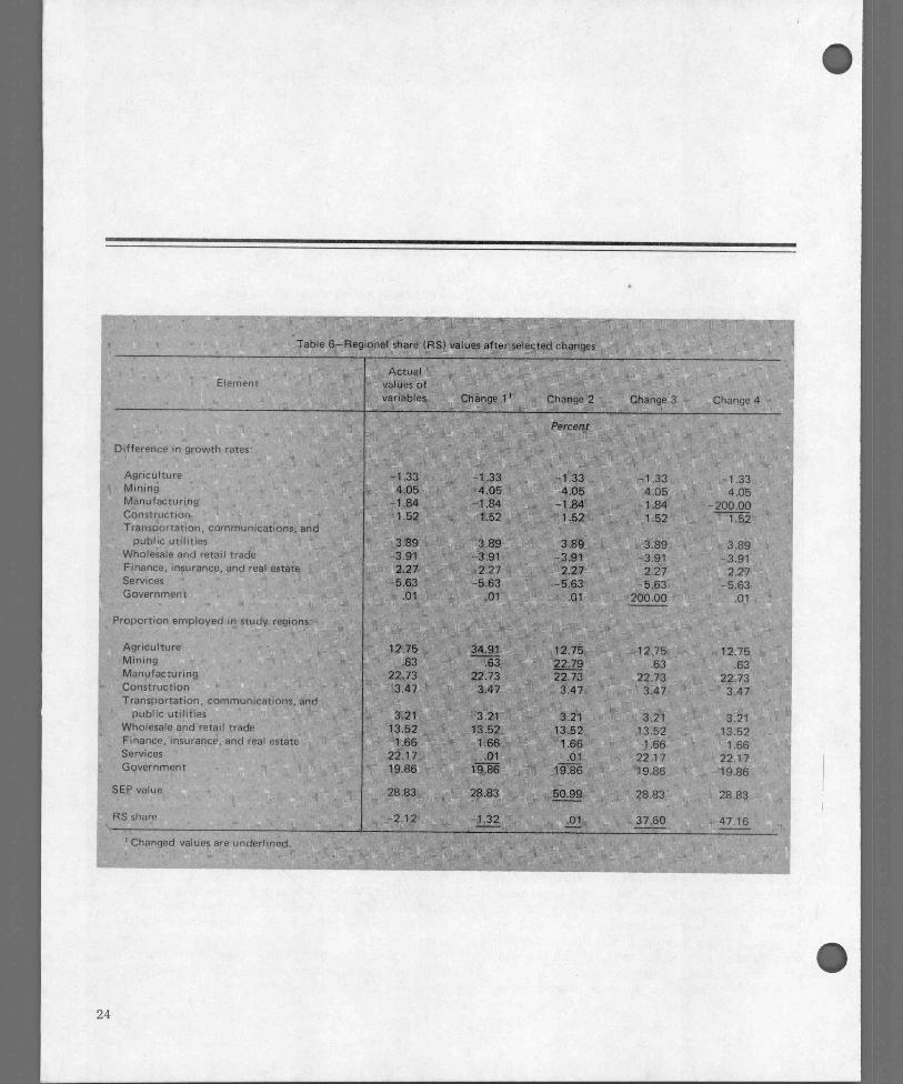
Table 6-Regional share (RS) values after selected changes

Element Actual

values of variables Change 1' Change 2 Change 3 Change 4

Difference in growth rates:

Percent

Agriculture -1.33 -1.33 -1.33 -1.33 -1.33 Mining 4.05 4.05 4.05 4.05 4.05 Manufacturing -1.84 -1.84 -1.84 -1.84 -200.00 Construction 1.52 1.52 1.52 1.52 1.52 Transportation, communications, and

public utilities 3.89 3.89 3.89 3.89 3.89 Wholeiale and retail trade -3.91 - 3.91 - 3.91 -3.91 -3.91 Finance, insurance, and real estate 2.27 2.27 2.27 2.27 2.27 Services -5.63 -5.63 -5.63 --5.63 -5.63 Government .01 .01 .01 200.00 .01

Proportion employed in study regions:

Agriculture 12.75 34.91 12.75 12.75 12.75 Mining .63 .63 22.79 .63 .63 Manufacturing 22.73 22.73 22.73 22.73 22.73 Construction 3.47 3.47 3.47 3.47 3.47 Transportation, communications, and

public utilities 3.21 3.21 3.21 3.21 3.21 Wholesale and'retail trade 13.52 13.52 13.52 13.52 13.52 Finance, insurance, and real estate 1.66 1.66 1.66 1.66 1.66 Services 22.17 .01 01 22.17 22.17 Government 19.86 19.86 19.86 19.86 19.86

SEP value 28.83 28.83 50.99 28.83 28.83

RS share -2.12 1.32 .01 37.60 -47.16

Changed values are underlined.

•

• 9.4

REFERENCES

nomic Growth: An Empirical Test." J. Regional Sci. Vol. 9, 1969.

"Shift and Share Pro-jections Revisited: A Reply." J. Regional Sci. Vol. 13, No. 1, 1973. Creamer, Daniel, "Shifts of Manufacturing Industries." In-dustrial Location and Natural Resources. U.S. Govt. Print. Off., Wash., D.C., 1943. Floyd, C. F., and C. F. Sirmans. "Shift and Share Projections Revisited." J. Regional Sci. Vol. 13, No. 1, 1973. Hellman, Daryl A. "Shift-Share Models As Predictive Tools." Growth and Change. Vol. 7, No. 3, 1976.

( 5)

•

(10) Houston, David B. "Shift and Share Analysis: A Critique." So. Econ. J. Vol. 32, 1967.

(11) Klaassen, L. H., and J. H. P. Pae-linck. "Asymmetry in Shift and Share Analysis." Regional and Urban Econ. Vol. 2, No. 3, 1972.

(12) Malizia, Emil. "Standardized Share Analysis." J. Regional Sci. Vol. 18, No. 2, 1978.

(13) Perloff, Harvey S., Edgar S. Dunn, Jr., Eric E. Lampard, and Richard F. Muth. Regions, Resources and Economic Growth. The Johns Hopkins Univ. Press, Baltimore, MD, 1960.

(14) Zimmerman, Rae. "A Variant of the Shift and Share Projec-tion Formulation." J. Regional Sci. Vol. 15, No. 1, 1975.

(1) Ashby, Lowell D. "The Geo-graphical Redistribution of Employment: An Examination of the Elements of Change." Suru. Current Business. Vol. 44, 1964.

(2) . Growth Patterns in Employment by County, 1940-50 and 1950-60. Off. Business Econ., U.S. Dept. Commerce, Wash., D.C., 1965.

(3) "The Shift and Share Analysis: A Reply." So. Econ. J. Vol. 33, No. 3, 1968.

(4) Bishop, K. C., and C. E. Simp-son."Components of Industrial Change Analysis: Problems of Alternative Approaches to In-dustrial Structure." Regional Studies. Vol. 6, 1972. Brown, H. J. "Shift and Share Projections of Regional Eco-

"Through this graphic twist to shift-share analysis, analysts can readily examine

composition and growth characteristics and the effects of change"

Merits of Graphic Approach

Through this graphic twist to shift-share analysis, analysts can readily examine composition and growth characteristics and the effects of change. The figures clarify how internal and external factors affect a region's growth components and its status with respect to other regions.

Planners will also find the graphic approach especial-ly useful, as it provides a well-structured vehicle for evaluating the impact of change. The approach may also be used simply to summarize a region's characteristics

for various time periods or to compare characteristics of numerous regions simultaneously.

CONCLUSIONS

This modified version of shift-share methodology, although not a predictive model, can be used to compare and appraise past and present economic growth patterns of regions. Regions can be classified objectively over time and their growth patterns can be compared over time and with one another.

25