Setting-less Protection: Centralized Substation Protection

Final Project Report

T-55G

Power Systems Engineering Research Center Empowering Minds to Engineer

the Future Electric Energy System

Setting-less Protection: Centralized Substation Protection

Final Project Report

Project Team A.P. Sakis Meliopoulos, Project Leader

George J. Cokkinides Georgia Institute of Technology

Graduate Students Hussain Albinali

Yuan Kong Boqi Xie

Jiahao Xie Chiyang Zhong

Georgia Institute of Technology

PSERC Publication 18-02

March 2018

For information about this project, contact:

A.P. Sakis Meliopoulos Georgia Institute of Technology School of Electrical and Computer Engineering Atlanta, Georgia 30332-0250 Phone: 404-894-2926 E-mail: sakis.m@gatech.edu

Power Systems Engineering Research Center

The Power Systems Engineering Research Center (PSERC) is a multi-university Center conducting research on challenges facing the electric power industry and educating the next generation of power engineers. More information about PSERC can be found at the Center’s website: http://www.pserc.org.

For additional information, contact:

Power Systems Engineering Research Center Arizona State University 527 Engineering Research Center Tempe, Arizona 85287-5706 Phone: 480-965-1643 Fax: 480-965-0745

Notice Concerning Copyright Material

PSERC members are given permission to copy without fee all or part of this publication for internal use if appropriate attribution is given to this document as the source material. This report is available for downloading from the PSERC website.

2018 Georgia Institute of Technology. All rights reserved.

i

Acknowledgements This targeted PSERC research project was funded by EPRI. We express our appreciation to EPRI, and especially to Paul Myrda, Technical Executive, for his support and guidance. We also express our appreciation for the support provided by PSERC’s industrial members, EPRI members, and the National Science Foundation’s Industry / University Cooperative Research Center program. The authors wish to recognize the postdoctoral researchers and graduate students at the Georgia Institute of Technology who contributed to the research and creation of project reports:

• Hussain Albinali • Yuan Kong • Boqi Xie • Jiahao Xie • Chiyang Zhong

ii

Executive Summary In recent years, there has been substantial technological progress of protective relays in substations. With the introduction of merging units and standards such as the IEC 61850, it is possible to formulate effective, reliable and self-healing centralized substation protection schemes. Such schemes utilize real-time measurements from various data acquisition equipment via standard communication protocols. These schemes perform single protective tasks (protection zone functions) and also supervise the health of the individual components of the protection system including instrumentation channel integrity, data integrity and software integrity. We refer to these schemes as centralized substation protection. Centralized substation protection can also enable condition based maintenance of protection and control systems. Setting-less protection based on dynamic state estimation is a promising technology to fulfill the objectives of centralized substation protection. The setting-less protection method was inspired from the fact that differential protection is one of the most secure protection schemes, which does not require coordination with other protection function. Differential protection simply monitors the validity of Kirchhoff’s current law in a device, i.e., the weighted sum of the currents going into a device must be equal to zero. This concept can be generalized into monitoring the validity of all other physical laws that the device must satisfy, such as Kirchhoff’s voltage law and Faraday's law. This monitoring can be done in a systematic way by use of dynamic state estimation. Dynamic state estimation (DSE) measures the consistency between measurements in the protection zone and its physical model. The method operates on measured sampled values. Accordingly, if the measurements do not fit the protection zone model, the relay detects a fault or abnormality. The DSE obtains the zone measurements in sampled value format via the process bus. The relay processes these measurements to perform dynamic state estimation in the time domain. This process determines how well the data fit the dynamic model by performing the chi-square test. Hidden failures in the instrumentation channels result in inaccurate measurements that will not fit the model of the zone under protection, even if no fault occurs in the system. Such failures could affect the scheme’s performance and cause relay mis-operation. Thus, a mechanism to detect such failures is essential for a reliable protection system. It should be noted that hidden failures affect the performance of any relaying scheme, not only setting-less relays. In prior research, numerical experiments and laboratory test based on the setting-less protection approach were performed on a number of protection problems, specifically, transmission line protection, capacitor bank protection, transformer protection, reactor protection, induction motor protection and distribution line protection. The research demonstrated that the dynamic state estimation approach provides a secure and dependable protection scheme, and does not require coordination with other devices or protection schemes while, at the same time, addresses many protection gaps. Following the above positive results previous study, the method has been extended to centralized substation protection. This report introduces a new dynamic state estimation-based centralized protection scheme (ebCSP) at the substation level. This system supplements dynamic state estimation-based protection for individual zones known as “setting-less relays” to secure their operation against hidden failures. The ebCSP communicates with the setting-less relays via the

iii

station bus and obtains essential information from each protection zone, such as phasor quantities, breakers, and disconnect status. This information is processed by the ebCSP to extract the substation topology and states. Specifically, the ebCSP performs dynamic state estimations in the quasi-dynamic domain once per cycle to detect any sort of abnormality within the substation. Upon detecting abnormalities, the ebCSP performs hypothesis testing to distinguish between faults and hidden failures. The ebCSP detects and locates hidden failures within the substation through hypothesis testing. Then, the ebCSP streams the estimated measurements that correspond to the detected bad measurements to the setting-less relay to replace the compromised measurement. Its capability to detect hidden failures and replace the compromised measurements in real time secure setting-less relays from mis-operation and ensure high dependability even with the presence of hidden failures. Such capability bridges a critical gap in protection systems. The integration of the proposed scheme and the individual zone protection form a resilient protection system that is self-immunized against hidden failures. The ebCSP concept has been tested with five numerical experiments:

• PT fuse blown • CT saturation • CT short circuit • CT reverse polarity • wrong CT ratio setting

The results show that setting-less protection is a viable approach to centralized substation protection. Project Publications: None Student Thesis:

]1[ Albinali Hussain. State Estimation-Based Centralized Substation Protection Scheme. Ph.D Dissertation, Georgia Institute of Technology, Atlanta GA, 2017.

iv

Table of Contents

1. Introduction .......................................................................................................................... 1

2. Review of Setting-less Protection ......................................................................................... 3

3. Implementation of ebCSP ..................................................................................................... 9

3.1 Measurement Model Extraction Module ........................................................................ 12

3.2 Substation-Wide Dynamic State Estimation Module ..................................................... 19

3.3 Hypothesis Testing Module ............................................................................................ 22

3.4 Data Correction Module ................................................................................................. 26

4. Numerical Experiments of ebCSP ....................................................................................... 27

4.1 Case 1: PT Fuse Blown .................................................................................................. 28

Scenario 1: Single Event, Fuse Blown of PT-4A without Fault ................................. 29

Scenario 2: Two Non-Concurrent Events, Fuse Blown of PT-4A and Phase to Phase Fault in the Distribution Line ...................................................................................... 34

Scenario 3: Two Concurrent Events, Fuse Blown of PT-4A and Phase to Phase Fault in the Distribution Line ............................................................................................... 42

4.2 Case 2: CT Short Circuit ................................................................................................ 45

Scenario 2: Concurrent events, CT-9A short circuit and power fault ......................... 48

4.3 Case 3: CT Saturation ..................................................................................................... 54

4.4 Case 4: CT Reverse Polarity ........................................................................................... 61

4.5 Case 5: CT Incorrect Ratio Settings ............................................................................... 65

5. Conclusion and future work ................................................................................................ 70

References ..................................................................................................................................... 71

v

List of Figures

Figure 2–1 Substation Level Setting-less Protective Relaying Overview ...................................... 3

Figure 2–2 Mechanism of Setting-less Protection Scheme for Components ................................. 4

Figure 2–3 Illustration of Setting-less Protection Logic ................................................................. 6

Figure 2–4 Setting-less Protection Relay Organization .................................................................. 7

Figure 2–4 Overall Approach for Component Protection............................................................... 8

Figure 3–1 Illustration of Overall Approach .................................................................................. 9

Figure 3–2 Synthesis of System Wide State Estimate from Substation State Estimates .............. 10

Figure 3–3 Architecture for Handling Sampled Values in the Substation .................................... 11

Figure 3–4 Architecture for Handling Phasor Data in the Substation .......................................... 11

Figure 3–5 Overall Architecture of the Proposed Scheme ........................................................... 12

Figure 3–7 Example Derived Measurements ................................................................................ 17

Figure 3-8 Illustration of circular buffer implementation for phasor extraction .......................... 19

Figure 3-8 Chi-square probability distribution function [11] ....................................................... 21

Figure 3-9 Flow chart of the hypothesis testing............................................................................ 25

Figure 3-10 breakdown of Time-delay for the setting-less relay. ................................................. 26

Figure 4–1 Example Test System for Numerical Experiments .................................................... 27

Figure 4–2 Single Line Diagram with Instrumentation ................................................................ 28

Figure 4–3 Outcome of the setting-less relay of the transformer zone for Scenario .................... 29

Figure 4–4 Voltage magnitude and angle from PT4 for Scenario ................................................ 30

Figure 4–5 The highest values of the normalized residual for Scenario 1 .................................... 31

Figure 4–6 The outcome of hypothesis testing for Scenario 1 ..................................................... 31

Figure 4–7 Hidden failure status in instrumentation channels for Scenario 1 .............................. 32

Figure 4–8 Setting-less relay corrected response for Scenario 1 .................................................. 33

Figure 4–9 Voltage and current waveforms of Distribution line zone side 1 for Scenario 2 ....... 35

Figure 4–10 Voltage and current waveforms of Distribution line zone side 2 for Scenario 2 ..... 35

Figure 4–11 setting-less relay response of the distribution line zone for Scenario 2 ................... 35

Figure 4–12 Setting-less relay output of the transformer zone for Scenario 2 ............................. 36

Figure 4–13 Voltage magnitude and phase angle of the distribution line side 1 for Scenario 2 .. 36

vi

Figure 4–14 Current magnitude and phase angle of the distribution line side 1 for Scenario 2 ... 38

Figure 4–15 Voltage magnitude and phase angle of PT 4 for Scenario 2 .................................... 38

Figure 4–16 The highest values of normalized residuals during the phase to phase fault for Scenario 2...................................................................................................................................... 39

Figure 4–17 The highest values of normalized residuals during the fuse blown event for Scenario 2..................................................................................................................................................... 39

Figure 4–18 The outcome of the hypothesis testing conducted by ebCSP for Scenario 2 ........... 40

Figure 4–19 Faulty zone identification for Scenario 2 ................................................................. 40

Figure 4–20 Hidden failure status in instrumentation channel for Scenario 2 ............................. 40

Figure 4–21 Corrected response of setting-less relay of transformer zone for Scenario 2 ........... 41

Figure 4–22 The highest values of normalized residuals for Scenario 3 ...................................... 43

Figure 4–23 The outcome of ebCSP for Scenario 3 ..................................................................... 44

Figure 4–24 Hidden failure status in instrumentation channels for Scenario 3 ............................ 44

Figure 4–25 Faulty zone identification from ebCSP for Scenario 3 ............................................. 44

Figure 4–26 Setting-less relay response for Scenario 1 ................................................................ 45

Figure 4–27 Highest values of normalized residual for Scenario 1 .............................................. 46

Figure 4–28 The ebCSP results for Scenario 1 ............................................................................. 47

Figure 4–29 Hidden failures identification for Scenario 1 ........................................................... 47

Figure 4–30 Setting-less relay corrected response for Scenario 1 ................................................ 48

Figure 4–31 Setting-less relay output of transformer zone for Scenario 2 ................................... 49

Figure 4–32 Setting-less relay output of distribution line zone for Scenario 2 ............................ 49

Figure 4–33 Current Phasor quantities from CT 9 of transformer Zone for Scenario 2 ............... 50

Figure 4–34 The highest values of the normalized residual for Scenario 2 .................................. 51

Figure 4–35 The outcome of ebCSP for Scenario 2 ..................................................................... 52

Figure 4–36 Faulty zone status for Scenario 2 .............................................................................. 52

Figure 4–37 Hidden failure status for Scenario 2 ......................................................................... 53

Figure 4–38 Corrected response of Setting-less relay of transformer zone for Scenario 2 .......... 54

Figure 4–39 The outcome of the setting-less relay of the transformer zone ................................ 55

Figure 4–40 The outcome of the setting-less relay of the transmission line without CT model .. 55

Figure 4–41 The outcome of the setting-less relay of the transmission line with CT model ....... 56

vii

Figure 4–42 Current phasor quantities of the primary side of the transformer ............................ 57

Figure 4–43 Current phasor quantities of the calculated primary side of CT-3 ........................... 58

Figure 4–44 The highest values of the normalized residual ......................................................... 58

Figure 4–45 The outcome of ebCSP ............................................................................................. 59

Figure 4–46 Hidden failure detection ........................................................................................... 59

Figure 4–47 Faulty zone detection ................................................................................................ 59

Figure 4–48 Corrected response of setting-less relay of transmission line zone .......................... 60

Figure 4–49 The outcome of the setting-less relay of the transformer zone ................................ 61

Figure 4–50 Angles of the Current waveform extratced from CT9 and CT 10 ............................ 62

Figure 4–51 The highest values of the normalized residual ......................................................... 63

Figure 4–52 The outcome of ebCSP ............................................................................................. 63

Figure 4–53 Hidden failure detections .......................................................................................... 63

Figure 4–54 Corrected response of setting-less relay of transformer zone .................................. 64

Figure 4–55 The outcome of the setting-less relay of the transformer zone ................................ 65

Figure 4–56 Magnitudes of the current phasor quantities of CT9 and CT 10 .............................. 66

Figure 4–57 The highest values of the normalized residual ......................................................... 67

Figure 4–58 The outcome of ebCSP ............................................................................................. 67

Figure 4–59 Hidden failure detections from ebCSP ..................................................................... 68

Figure 4-60 Corrected response Setting-less relay of transformer zone ....................................... 69

1

1. Introduction

Protection and control systems (P&C) around the world are experiencing an evolution driven by the introduction of new technologies. At the same time, P&C systems are called to protect and control an ever-evolving power system with many new complexities arising from new energy resources, particularly renewable energy resources, power electronics conversion systems and high-voltage direct current (HVDC) transmission. According to a recent forecast, renewable energy resources will comprise around 31.2% of total world power generation by 2035. A significant portion of these resources will come from wind and solar energy [[1]]. This massive deployment of new energy resources has already led to several changes in power system characteristics, including reduced fault current levels [[2]], increased dynamics and wider frequency variations to disturbances. Legacy [protection systems are typically depending on large separation between load current and fault currents. This condition is disappearing in parts of the system. In general, these changes mandate new approaches to deal with the protection and control of the modern power system. Advances in P&C technologies have increased the complexity of protection and control systems. Complexity increases the possibility of errors and reduces protection reliability. As a result, despite the great technological advances, protection mis-operations are at undesirable levels. Relay mis-operations levels are at approximate levels of 10%, as reported by the North American Electric Reliability Corporation (NERC) for the USA. Similar statistics exists for many other parts of the world. Further analysis of misoperation statistics indicates that around 65% of mis-operations are caused by settings, logic errors, mis-coordination and communications failures. These causes are characterized as hidden failures, which are defined as “permanent defect(s) that will cause a relay or a relay system to incorrectly and inappropriately remove a circuit element(s) as a direct consequence of another switching event”. This definition implies that hidden failures cause incorrect interruption to a portion of power systems because of a fault to another part of the network. Consequently, they may initiate second level contingencies in the power system network and possibly a cascading effect. In any case, relay mis-operations drastically affect power system reliability. Present day numerical relays have a limited capability to detect hidden failures and no capability to recover unless repair is performed. In addition, if a hidden failure occurs simultaneously with a fault in the system, present day relays are not capable of identifying this condition and the response of the relay could most likely be a mis-operation. In any case, if a present day relay detects a hidden failure the only option is to inhibit the protection function and rely on backup protection for the protection of the system. Specifically, the affected protection system will depend on other protection systems, unaffected by the hidden failure(s), to take the proper action. It should be apparent the protection system reliability is decreased. Relay manufacturers and researchers have proposed approaches that could minimize the effects of hidden failures and cope with other complexities. Along these lines, adaptive protection schemes and voting schemes have been proposed. Adaptive protection schemes have been proven to be complex and do not easily meet the speed that is required for protection. Voting schemes are not reliable as a hidden failure may affect several relays that participate in the voting – in this case the majority of relays may be taking a wrong decision.

2

Technology advancements have played a major role in paving the way for a new protection system capable of overcoming present day challenges. Specifically, the introduction of merging units, advancements in computational capabilities and the communication infrastructure as well as related standards enables the realization of centralized approaches for supervision of protective functions and self-healing and self-correction of the effects of hidden failures until physical repair takes place. The introduction of IEC 61850 provides the blue print to allow IEDs from various manufactures to seamlessly participate in new protection schemes. Data transfer within the substation protection and control equipment has been standardized for any application. The health of the protection and control system itself is of paramount importance for the reliability of the power grid. Today, the technology to monitor the condition of the protection and control system exists, however the methods are not well developed. There are several aspects of this problem: (a) the health and accuracy of the instrumentation, (b) the accuracy of relay settings, and (c) the condition and speed of the communications. We describe new approaches to address the issue of condition monitoring of the entire protection and control system of a substation. A dynamic state estimation based Centralized Substation Protection scheme is proposed (ebCSP), which supervises the protective relays for individual zones, detects hidden failures and corrects compromised data resulting from hidden failures. The preferred implementation of the proposed scheme uses an infrastructure of merging units and setting-less protective relays. The ebCSP monitors the operation of all protection zones in the substation, using data obtained from setting-less relays, detects data abnormalities, including hidden failures and most importantly, in case of hidden failures corrects compromised data so that the protection zones can properly operate. The proposed centralized protection scheme, along with setting-less relays, forms a resilient substation-centralized protection system capable of mitigating the limitation in conventional protection systems, including the protection of power electronic–based systems and the capability of detecting hidden failures. Descriptions of the constituent parts of the approach are provided next.

3

2. Review of Setting-less Protection

A new approach for zone protection has been introduced recently. The approach uses dynamic state estimation to determine whether a protection zone is experiencing a fault. It has been given the name “setting-less relay” because the settings are extremely simplified and requires no coordination with any other protection functions. Two pilot research projects were focused on field testing of this technology. The relay of each zone monitors the consistency between all physical laws, which the zone under protection must satisfy, and measurements taken in and around a protection zone. This process is mathematically formulated as a dynamic state estimation (DSE), which provides a quantitative assessment of how well the measurements of the zone fit its dynamic model in real time. A preferred implementation is to use merging units to obtain measurements which are streamed to the setting-less relay through a process bus. The measurements are processed with a dynamic state estimation which computes the best estimate of the protection zone states. It also computes the goodness of fit or the probability that the measurements “fit” the zone model within the accuracy of the metering used (via the well-known chi-square test). A low probability indicates abnormalities/faults in the protection zone. The chi-square test typically returns a probability of 100% for healthy protection zones and 0% for a protection zone with any type of internal fault. Setting-less relays have many advantages over conventional protection schemes: (a) they do not require coordination with any other relay functions, and (b) they can detect the fault much faster (i.e., within a few samples which translates to less than one millisecond) than conventional protection schemes. The complexity of protection schemes is greatly simplified. A schematic of the substation protection scheme where all protection zones are protected by a setting-less relay using merging units, is shown in Figure 2-1.

Figure 2-1: Schematic of Substation Level Setting-less Protective Relaying The organization of each setting-less protective relay is shown in Figure 2-2. Note that this general arrangement applies to any protection zone.

4

Figure 2-2: Organization of Setting-less Protective Relay for a Protection Zone The setting-less protection method has been inspired from the fact, that differential protection is one of the most secure protection schemes that we have and it does not require coordination with other protection function. Differential protection simply monitors the validity of Kirchhoff’s current law in a device, i.e., the weighted sum of the currents going into a device must be equal to zero. This concept can be generalized into monitoring the validity of all other physical laws that the device must satisfy, such as Kirchhoff’s voltage law, Faraday's law, etc. This monitoring can be done in a systematic way by the use of dynamic state estimation. Specifically, all the physical laws that a component must obey are expressed in the dynamic model of the component. Dynamic state estimation is used to continuously monitor the dynamic model of the component (zone) under protection. If any of the physical laws for the component under protection is violated, the dynamic state estimation will capture this condition. Thus, it is proposed to use dynamic state estimator to extract the dynamic model of the component under protection [3-10] and to determine whether the physical laws for the component are satisfied. The dynamic model of the component accurately reflects the condition of the component and the decision to trip or not to trip the component is based on the condition of the component only irrespectively of the condition (faults, etc.) of other system components. The proposed method requires a monitoring system of the component under protection that continuously measures terminal data (such as the terminal voltage magnitude and angle, the frequency, and the rate of frequency change - this task is identical to present day numerical relays), other variables such as temperature, speed, etc., as appropriate, and component status data (such as the tap setting, breaker status, etc.). The dynamic state estimation processes these measurements and extracts the real time dynamic model of the component and its operating

5

conditions. An illustrative description for the protection of a single component is provided in Figure 2–2. After estimating the operating conditions, the well-known chi-square test [8] calculates the probability that the measurement data are consistent with the component model, i.e., the physical laws that govern the operation of the component. In other words, this probability, which indicates the confidence level of the goodness of fit of the component model to the measurements, can be used to assess the health of the component. The high confidence level indicates a good fit between the measurements and the model, which indicates that the operating condition of the component is normal. However, if the component has internal faults, the confidence level would be almost zero (i.e., the very poor fit between the measurement and the component model). Figure 2–2 shows the concept of entire proposed protection for a single component. In general, the proposed method can identify any internal abnormality of the component within a cycle and trip the component immediately. Furthermore, it does not degrade the security because a relay does not trip in the event of normal behavior of the component, for example, in case of transformer protection, inrush currents or over excitation currents, since in these cases, as long as the inrush currents are consistent with the transient behavior of the transformer as dictated by the dynamic model, the method will produce a high confidence level that the transients are consistent with the model of the component. Note also that the method does not require any settings or any coordination with other relays. It is important to note that the proposed scheme will perform best when: (a) the measurements are as accurate as possible - dependent on the type of instrument transformer used, i.e., VT, CT, etc. and the instrumentation channel, i.e., control cable, etc. and (b) the accuracy of the dynamic model of the component under protection. These issues, while important, are beyond the scope of this report. These issues will be addressed in a subsequent report.

6

Figure 2-3: Generic Description of Setting-less Protection Logic The proposed protection logic is briefly illustrated in Figure 2–3. The method requires a monitoring system of the component under protection that continuously measures terminal data (such as the terminal voltage magnitude and angle, the frequency, and the rate of frequency change) and component status data (such as tap setting and temperature for transformers). The dynamic state estimation processes these measurement data with the dynamic model of the component yielding the operating conditions of the component. The implementation of the setting-less relays has been approached from an object-oriented point of view. For this purpose, the constituent parts of the approach have been evaluated and have been abstracted into a number of objects. Specifically, the setting-less approach requires the following objects:

1. the mathematical model of the protection zone 2. the physical measurements that may consist of analog and digital data 3. the mathematical model of the physical measurements 4. the mathematical model of the virtual measurements 5. the mathematical model of the derived measurements 6. the mathematical model of the pseudo measurements 7. the dynamic state estimation algorithms 8. the bad data detection and identification algorithm 9. the protection logic and trip signals 10. online parameter identification method

7

An overview of the design of the setting-less protection relay is shown in Figure 2–4.

Figure 2-4: Setting-less Protection Relay Organization This approach faces some challenges which can be overcome with present technology. A partial list of the challenges is given below:

1. Ability to perform the dynamic state estimation in real time 2. Initialization issues 3. Communications in case of a geographically extended component (i.e., lines) 4. New modeling approaches for components - connects well with the topic of modeling

requirement for GPS synchronized measurements in case of multiple independent data acquisition systems.

5. Other The modeling issue is fundamental in this approach. For success, the model must be high fidelity so that the component state estimator will reliably determine the operating status (health) of the component. For example, consider a transformer during energization. The transformer will experience high in-rush current that represent a tolerable operating condition and therefore no relay action should occur. The component state estimator should be able to "track" the in-rush current and determine that they represent a tolerable operating condition. This requires a transformer model that accurately models saturation and in-rush current in the transformer. We can foresee the possibility that a high-fidelity model used for protective relaying can be used as the main depository of the model which can provide the appropriate model for other applications. For example, for EMS applications, a positive sequence model can be computed from the high-fidelity model and send to the EMS data base. The advantage of this approach will be that the EMS model will come from a field validated model (the utilization of the model by the relay in real time provide the validation of the model). This overall approach is shown in Figure 2.4. Since protection is ubiquitous, it makes economic sense to use relays for distributed model data base that provides the capability of perpetual model validation.

Protection Zone SACQCF model

MeasurementDefinition

• Create Actual Measurement Model

• Create Virtual Measurement Model

• Create Pseudo Measurement Model

• Create Derived Measurement Model

SCAQCF Measurement Model

Setting-less Protection

Dynamic State Estimation

Error Analysis Bad Data

Detection & Identification

Model Parameter

Identification

Future

ProtectionLogic

Merging Unit

Merging Unit

Merging Unit

DataConcentrator

8

Figure 2-4: Protection Zone Model Validation and Interfaces to Other Power System Operations As any relaying scheme, setting-less relays are also vulnerable to hidden failures. Hidden failures will cause errors in the protection logic whether a legacy protection function or setting-less relay. It follows that hidden failures are critical and undermine protection reliability. Methods to detect such failures are essential for reliable protection of power system components. We propose a estimation based centralized substation protection (ebCSP) scheme to supervise all setting-less relays in a substation to secure their operation against hidden failures.

9

3. Implementation of ebCSP

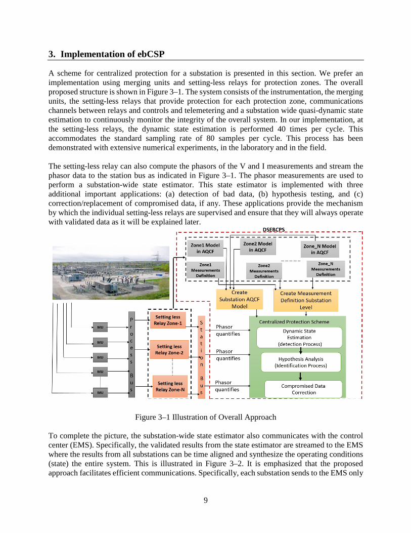
A scheme for centralized protection for a substation is presented in this section. We prefer an implementation using merging units and setting-less relays for protection zones. The overall proposed structure is shown in Figure 3–1. The system consists of the instrumentation, the merging units, the setting-less relays that provide protection for each protection zone, communications channels between relays and controls and telemetering and a substation wide quasi-dynamic state estimation to continuously monitor the integrity of the overall system. In our implementation, at the setting-less relays, the dynamic state estimation is performed 40 times per cycle. This accommodates the standard sampling rate of 80 samples per cycle. This process has been demonstrated with extensive numerical experiments, in the laboratory and in the field. The setting-less relay can also compute the phasors of the V and I measurements and stream the phasor data to the station bus as indicated in Figure 3–1. The phasor measurements are used to perform a substation-wide state estimator. This state estimator is implemented with three additional important applications: (a) detection of bad data, (b) hypothesis testing, and (c) correction/replacement of compromised data, if any. These applications provide the mechanism by which the individual setting-less relays are supervised and ensure that they will always operate with validated data as it will be explained later.

Figure 3–1 Illustration of Overall Approach To complete the picture, the substation-wide state estimator also communicates with the control center (EMS). Specifically, the validated results from the state estimator are streamed to the EMS where the results from all substations can be time aligned and synthesize the operating conditions (state) the entire system. This is illustrated in Figure 3–2. It is emphasized that the proposed approach facilitates efficient communications. Specifically, each substation sends to the EMS only

10

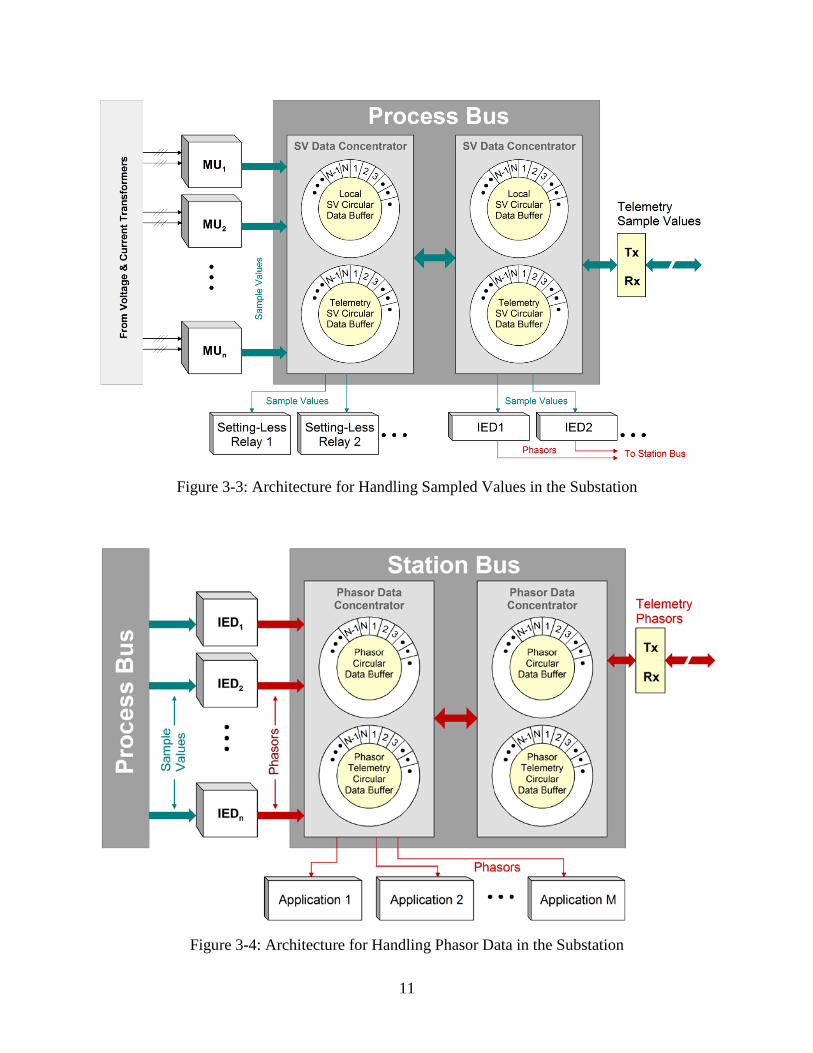
its real-time model which comprises a very small number of data. When connectivity changes, then connectivity data are transmitted by exception. Similarly, if model changes occur, the new mathematical model will be transmitted by exception. The end result is that while the merging units in a substation may be collecting data at rates of millions of data points per second, the frequency domain state (phasors) are only a few tens of data points per second and per substation. In order to better accommodate the seamless operation of each function of the system, the architecture of the system should be streamlined. Figure 3–3 and Figure 3–4 illustrate the architecture with emphasis on the data flow and data handling. Figure 3–3 shows the architecture to deal with sample values. Note that all SV are concentrated on four circular buffers which are handled with the sample value data concentrator (SVDC). The four circular buffers handle the local SVs and the telemetered SV with full redundancy. The SVDC time aligns the SVs as they may be coming from the various merging units with different time latencies and orders them in the circular buffer. Figure 3–4 shows a similar architecture for phasor data. The scheme accommodates local phasor data as well as telemetered phasor data. Finally, Figure 3–5 shows the overall architecture.

Figure 3–2 Synthesis of System Wide State Estimate from Substation State Estimates

11

Figure 3-3: Architecture for Handling Sampled Values in the Substation

Figure 3-4: Architecture for Handling Phasor Data in the Substation

12

Figure 3-5: Overall Architecture of the Proposed Scheme

The centralized protection scheme consists of four main modules, as shown in Figure 3–1. The first module is measurement model extraction, which extracts the phasor measurement model from the merging units setup file and the sampled values at the process bus. The second module is the DSE module, which performs DSE at the substation level to detect data abnormalities. The third module is the hypothesis testing module, which identifies the cause of data abnormalities in real time (hidden failures or faulty power system components). The fourth module is the compromised data correction/replacement module, which corrects/replaces compromised data with estimated data to enable the secure and dependable operation of the setting-less relays. Note that the third and fourth modules are executed only when an abnormality has been detected. Brief descriptions of each module are provided next.

3.1 Measurement Model Extraction Module

The measurement model for the substation wide dynamic state estimator is needed in phasor form and it is computed from the sample values at the process bus and the measurement definition included in the merging unit setup. Note that the so-extracted phasor measurements correspond one-to-one with the measurements collected at the merging units. The implementation of the measurement computation in phasor domain has been implemented in an object-oriented manner. We have developed a standard syntax for models and measurements which has been named State Control and Parameter Algebraic Quadratic Companion Form (SCPAQCF). The SCPAQCF is a mathematical model derived from the physical model of each power system device in the

13

substation, including the interconnecting circuits. Using the device model, the SCAQCF syntax of the measurements is computed. The SCPAQCF model and measurement development process has the following steps. Step 1: The Compact Device Model: The first step is to write the mathematical model equations for the physical power device under consideration. We refer to it as the compact device model and consists of a set of algebraic and differential equations that are linear and/or nonlinear. This is the usual way that one models a power device. Step 2: The SCPQDM Device Model: The second step is the quadratization step and it is invoked when the device compact model exhibits nonlinearities higher than two. This step is achieved by introducing new state variables. The end result is that the model consists of linear and possibly quadratic terms. The variables appearing in this form are the states of the model, the control variables of the model and the parameters of the model. The model in this format is referred to as the State, Control and Parameter Quadratized Dynamic Model (SCPQDM). The state, control and parameter quadratized device model is presented here. The specific syntax of the model has been developed under the following requirements: (a) all external equations, which include through variables, are linear differential equations and they are listed first; (b) the remaining (internal) equations are structured as follows: (b1) all equations that include differential terms are converted into linear equations and listed first together with the linear internal equations; (b2) the remaining equations are quadratic equations and are listed next. In addition, the state variables should be ordered as follows: (1) the interface states are listed first and should be corresponding to through variables; (2) the remaining state variables should be ordered so that should make the equations diagonal dominant, if possible. The standard time domain quadratized model is shown below:

1 1 1 1 1

2 2 2 2 2

3 3 3 3 3

( )( ) ( ) ( ) ( )

( )0 ( ) ( ) ( )

0 ( ) ( ) ( ) ( ) ( ) ( ) ( ) ( )

eqx equ eqp eqxd eqc

eqx equ eqp eqxd eqc

T i T ieqx equ eqp eqxx equu

d ti t Y t Y t Y t D Cdt

d tY t Y t Y t D Cdt

Y t Y t Y t t F t t F t t

= + + + +

= + + + +

= + + + + +

xx u p

xx u p

x u p x x u u p

3

3 3 3 3

( )

( ) ( ) ( ) ( ) ( ) ( )

T ieqpp

T i T i T iequx eqpx equp eqc

F t

t F t t F t t F t C

+ + + +

p

u x p x u p

14

( , , )

T i T i T ifeqx fequ feqp feqxx fequu feqpp

T i T i T ifequx feqpx fequp feqc

Y Y Y F F F

F F F C

= + + + + +

+ + + +

h x u p x u p x x u u p p

u x p x u p

Step 3: The SCPAQCF Model: The third step involves a numerical integration of the SCPQDM. The method we use is the quadratic integration method which assumes that the variables vary quadratically over the integration time step. The end result of the quadratic integration is the SCPAQCF. Note that SCPAQCF model consists of algebraic equations only as the dynamics of the model (differential terms) have been converted into algebraic equation with “past history”. Note that other numerical integration methods can be used. We found the quadratic integration has very nice properties and is not too complex. The mathematical details of this process can be found in previous publications. The end result is an algebraic companion form that is a set of linear and quadratic algebraic equations that are cast in the following standards form:

( )00

( ) ( ) ( ) ( ) ( ) ( ) ( ) ( ) ( )( )00

( ) ( ) ( ) (

T i T i T ieqx equ eqp eqxx eqpp equu

m

T i T iequx equp

i t

Y t Y t Y t t F t t F t t F ti t

t F t t F

= + + + + +

+ +

x u p x x p p u u

u x u p ) ( ) ( )T ieqpx eqt t F t B

+ −

p x

(1)

and ( ) ( ) ( ) ( )eq eqx equ eqp eq eqB N t h N t h N t h M i t h K= − − − − − − − − −x u p (2)

where ( )( ), mi t i t is the through variable (current) vector, [ ( ), ( )]mt t=x x x is the external and

internal state variables, [ ( ), ( )]mt t=u u u is the control variables, t is present time, tm is the midpoint between the present and previous time, Yeq is an admittance matrix, Feq are the nonlinear matrices.

15

Step 4: The SCPQDM Measurement Model: Any measurement is a function of the state, control and parameter vector. The quadratized model results in the following general quadratized model of a measurement.

( )( ) ( ) ( )z z z zd tz t Y t Y t D C

dt= + + +

xx u

The model also includes the measurement noise error: dMeterScale, dMeterSigmaPU Step 5: The SCPAQCF Measurement Model: The quadratized measurement model is integrated with the quadratic integration method to provide the SCPAQCF model of the measurement. The SCPAQCF measurement model has the following form:

, , , , ,T i T i T i

m x m x m u m u m ux mY F Y F F C = + + + + +

z x x x u u u u x

, ,( ) ( ) ( )m m x m u m mC N t h N t h M z t h K= − + − + − +x u

dMeterScale, dMeterSigmaPU where [ ( ), ( )]mz z t z t= is the measurement vector, [ ( ), ( )]mt t=x x x is the external and internal state

variables, [ ( ), ( )]mt t=u u u is the control variables, t is present time, tm is the midpoint between the present and previous time, the indicated matrices are dependent upon the parameters appearing in the measurement quadratized model. This model is expressed in sparsity mode and has the following form:

, , , , , ,, , ,

k k k k k kj eqx i i eqx ij i j equ i i equ ij i j eqxu ij i j eq i

i i j i i j i j iz Y x F x x Y u F u u F x u b= ⋅ + ⋅ ⋅ + ⋅ + ⋅ ⋅ + ⋅ ⋅ −∑ ∑ ∑ ∑ ∑ ∑

In general the measurements can be identified as: (a) actual measurements, (b) virtual measurements, (c) derived measurements and (d) pseudo measurements. The types of measurements will be discussed next. Actual Measurements: In general, the actual measurements can be classified as across and through measurements. Across measurements are measurements of voltages or other physical quantities at the terminals of a protection zone such as speed on the shaft of a generator/model. These quantities are typically states in the model of the component. For this reason, the across measurements has a simple model as follows:

j i j jz x x η= ± + . (3)

Through measurements are typically currents at the terminals of a device or other quantities at the terminals of a device such as torque on the shaft of a generator/motor. The quantity of a through measurement is typically a function of the state of the device. For this reason, the through

16

measurement model is extracted from the algebraic companion form, i.e., the measurement model is simply one equation of the SCACQF model, as follows:

, , , , , ,, , ,

k k k k k kj eqx i i eqx ij i j equ i i equ ij i j eqxu ij i j eq i

i i j i i j i j iz Y x F x x Y u F u u F x u b= ⋅ + ⋅ ⋅ + ⋅ + ⋅ ⋅ + ⋅ ⋅ −∑ ∑ ∑ ∑ ∑ ∑ , (4)

where the superscript k means the kth row of the matrix or the vector. Virtual Measurements: The virtual measurements represent a physical law that must be satisfied. For example, we know that at a node the sum of the currents must be zero by Kirchhoff’s current law. In this case we can define a measurement (sum of the currents); note that the value of the measurement (zero) is known with certainty. This is a virtual measurement. The model can provide virtual measurements in the form of equations that must be satisfied. Consider for example the mth SCAQCF model equation below:

, , , , , ,, , ,

0 k k k k k keqx i i eqx ij i j equ i i equ ij i j eqxu ij i j eq i

i i j i i j i j iY x F x x Y u F u u F x u b= ⋅ + ⋅ ⋅ + ⋅ + ⋅ ⋅ + ⋅ ⋅ −∑ ∑ ∑ ∑ ∑ ∑ (5)

This equation is simply a relationship among the states the component that must be satisfied. Therefore, we can state that the zero value is a measurement that we know with certainty. We refer to this as a virtual measurement. Derived Measurements: A derived measurement is a measurement that can be defined for a physical quantity by utilizing physical laws. An example derived measurement is shown in Figure 3–7. The figure illustrates a series compensated power line with actual measurements on the line side only. Then derived measurements are defined for each capacitor section. Note that the derived measurements enable the observation of the voltage across the capacitor sections.

17

dd

A B Cva vb vc

vmi

ia ib ic

iam ibm icm

mq

n

mq

mq

n

mq

mq

n

mq

d

cc

C C C

C C C

R

L

N vn

in

Rg

Actual Measurement

Derived Measurement

Derived Measurement

ii

Figure 3–7 Example Derived Measurements Pseudo Measurements: Pseudo measurements are hypothetical measurements for which we may have an idea of their expected values but we do not have an actual measurement. For example, a pseudo measurement can be the voltage at the neutral; we know that this voltage will be very small under normal operating conditions. In this case we can define a measurement of value zero but with a very high uncertainty. Summary: Eventually, all the measurement objects form the following measurement set:

( ) ( ) ( ) ( ) ( ) ( )( )

, T T T Tm m

m

x tz h x t c a x t b x t x t x t F

x tη η

= + = + + + +

, (6)

where z is the measurement vector, x the state vector, h the known function of the model, a, b are constant vectors, F are constant matrices, and η the vector of measurement errors. Phasor Extraction: The ebCSP performs dynamic state estimation in the quasi-dynamic domain, which is the domain that neglects electrical transient phenomena and uses phasor quantities. Therefore, phasor quantities need to be computed from the sample values used in the setting-less relay. These phasor quantities have been computed using Fourier series expansion, which allows us to express the sampled waveform x(t) as follows: ( ) ( ) ( )1 2cos sinx t a t a t harmonicsω ω= + +

18

To compute the parameters a1 and a2 efficiently, we propose using the circular array-based algorithm as illustrated in Figure 3-8 [13]. To explain the algorithm, consider a sampled value of x(i) and two sets of circular arrays with N entries each. The entries of the circular buffers are initialized to zero. Then the process starts by computing the values y(i) and z(i) for each sampled value as follows:

0( ) ( )cos( )y i x i W Ti=

0( ) ( )sin( )z i x i W Ti= where x(i) is the sampled value at sample i, W0 is the base frequency, and T is the period of the sampled waveform. After each sample, the values of V1(k) and V2(k) are computed as follows:

( )1

1( )

k N

i kV k y i

+ −

== ∑

2

1( ) ( )

k N

i kV k z i

+ −

== ∑

For each new sample beyond the first N samples, the values V1(k) and V2(k) are updated as follows:

1 1( ) ( 1) ( ) ( )V k V k y i y i N= − + − −

2 2( ) ( 1) ( ) ( )V k V k z i z i N= − + − − where ( )y i N− and ( )z i N− are the oldest values in the circular buffer that will be overwritten by introducing the latest values of ( )y i and ( )z i . Finally, the phasor values are computed as follows:

2( ) ( ( ) ( ))1 2x k V k V kN= +

19

Figure 3-8 Illustration of circular buffer implementation for phasor extraction

3.2 Substation-Wide Dynamic State Estimation Module

The substation-wide dynamic state estimation module operates on the entire measurement set of the substation. No other information is needed. The DSE computes the best estimate of the substation dynamic state. Subsequently, the goodness of fit between the measurements and the substation model is computed via the well-known chi-square test which calculates the probability of goodness of fit between the measurement and the substation model. This probability is also referred to as confidence level. A high probability of goodness of fit, i.e. more than 0.90 results in declaring all the data in the substation valid. In this case no further action is required. Otherwise, the hypothesis module is called to identify the root cause of the bad data via hypothesis testing and correct/replace compromised data. In the proposed scheme, the dynamic state estimation method is used to compute the best estimate of the state variables for the substation. These computed states are used to calculate the estimated measurement using the substation model. The state estimation performance is analyzed through a chi-square test, which measures the goodness of fit between the measurements and the substation model. The goodness of fit is quantified by what is known as the confidence level. Therefore, a high confidence level indicates that the measurements’ fit with the model and the substation is healthy. The following subsection details the process of the dynamic state estimation formulations.

20

Weighted Least-Square Method We have used the weighted least-square method to formulate the dynamic state estimation at the substation level. This formulation is started by expressing the measurements in terms of the state variables of the substation as follows:

( ) ( ) , ,T iz t h x Y F Cqm x qm x qmk k η η

= + = + + +

x x x

where z is the measurements; 𝑥𝑥 is the state variables; Yqm, x is the coefficient matrix of the linear terms; Fqm,x is the coefficient matrix of nonlinear terms; Cqm is the constant term; and 𝜂𝜂 is the measurement error. Then the WLS method is formulated as an optimization problem with an objective function to minimize the error as follows [11], [12], [15]:

where 𝑠𝑠𝑖𝑖 = η𝑖𝑖𝜎𝜎𝑖𝑖

, 𝑊𝑊 = 𝑑𝑑𝑑𝑑𝑑𝑑𝑑𝑑 �⋯ , 1𝜎𝜎𝑖𝑖2 ,⋯�, and 𝜎𝜎𝑖𝑖 is the standard deviation of the meter by which the

corresponding measurement 𝑧𝑧 is measured. For the nonlinear case, the solution is given with Newton’s iterative algorithm as follows: 1 1( ) ( ( ) )V V T T vx x H WH H W h x z+ −= − −

where 𝐻𝐻 is the Jacobean matrix computed as follows: ( )h xH x

δδ=

For the linear case, the solution is given as follows: 1( ) ( )T TX H WH H W Z C−= − .

Abnormality Detection Abnormality detection is achieved by performing the chi-square test, which calculates the goodness of fit between the measurement and the substation model. The goodness of fit is quantified by the confidence level. A high confidence level indicates a healthy substation, and a low confidence level indicates an abnormality. The chi-square test is computed as follows [11],

22

1 1

( )n nTi i

ii ii

h x zMinimize J s Wη ησ= =

−= = =

∑ ∑

21

2

0

( ) ( )( )n

k k

k

h x Z tξδ=

−= ∑

V m n= − 2Pr( ) ( , )P Vχ ξ ξ≤ = Confidence level= 2Pr( ) 1 ( , )P Vχ ξ ξ≥ = −

where the variable is the summation of normalized residuals, which have a Gaussian distribution within the range of –1 to 1. The variable V represents the degree of freedom, which is the difference between the number of the measurement (m) and the number of the states (n). The term is the chi-square probability distribution function, which is shown in Figure 3-8. It represents the probability that the summation of the normalized residuals is out of the bounds. In fact, it is the probability that the measurements do not fit the model. Accordingly, this probability is used to compute the confidence level which is the probability that the measurements fit the substation model.

Figure 3-8 Chi-square probability distribution function [11]

ξ

2Pr( )χ ξ≤

22

3.3 Hypothesis Testing Module

This module is initiated when the dynamic state estimation has declared the existence of bad data (data abnormality). The objective of this module is to identify the root cause of the abnormality, i.e. power fault or hidden failure. There exist three possibilities: (a) one or more power faults exist in the system, (b) one or more hidden failures, or (c) simultaneous occurrence of faults and hidden failures. The probability of having two simultaneous faults or two simultaneous hidden failures within the substation is very low. Realistically, one should consider the following possible events as most likely to occur: (a) occurrence of a hidden failure, (b) occurrence of a power fault, and (c) simultaneous occurrence of a power fault and a hidden failure. Other possible events will have insignificant probabilities of occurring simultaneously. The hypothesis testing is guided by the following observations: (a) at the substation level the redundancy is high (over 2000%) – this implies that the existence of leveraging points are not existent and therefore normalized residuals from the state estimator can be used as guidance of where the problem is located. (b) System is continuously running – this implies that any abnormal event will be captured in real time. The probability of simultaneous failure events occurring at exactly the same tie is low. Thus, the hypotheses to be considered should be limited to first order events. To identify the type and location of the abnormality, we propose using hypothesis testing. The enabler for such approach is the high redundancy in the measurements at the substation level. This redundancy minimizes the possibility of leverage point. Therefore, the measurements with abnormality will always experience higher residual error than the healthy ones. Accordingly, the hypothesis testing starts by characterizing the measurements as suspect based on the values of their normalized residuals. Typically, the measurements with the highest normalized residual are considered as suspicious measurements. The Normalized residual is computed during the DSE computation with:

( )ˆi ii

i

h x znr

σ−

=

where inr is the normalized residual for measurement i, ( )ˆih x is the calculated measurement using the estimated substation states, iz is the measurement i, and iσ is the standard deviation of the meter error. To classify the abnormality to either hidden failure or power fault we introduce the concept of device common mode criteria which enables grouping multiple suspicious measurements into one set if they are modeled by a single device and their normalized residuals exceed threshold of 2. There are two device common mode criteria; (1) a zone common mode criterion which allows grouping all the measurements associated with a zone, for which setting-less relay is operated, into a one set of suspicious measurements if their normalized residuals exceed 2. and (2) an instrumentation channel common mode criterion which enables grouping the measurements extracted from an instrumentation channel if their normalized residual exceed threshold of 2. Our design considers three types of hypotheses.

23

Hypothesis Type 1 (H1): Remove suspect measurements and rerun DSE. If probability is high (more than 0.9), then: (a) removed measurements are bad, (b) identify root cause, (c) issue diagnostics, and (d) replace bad data with estimated values. End hypothesis testing. Otherwise go to H2. Hypothesis Type 2 (H2): (determine if a fault decision is correct). For the reported faulted device, remove all internal device measurements and remove the faulted device model from the substation model. Then rerun DSE. If probability is high (more than 0.9), then: (a) the device/protection zone is truly experiencing an internal fault. Allow zone relay to trip the faulted device. End hypothesis testing. Hypothesis Type 3 (H3): This test combines type 1 and type 2 hypothesis testing to cover the case of a simultaneous fault and a hidden failure. The first hypothesis considers bad measurements only as a result of hidden failure. This hypothesis involves selecting the measurement with the highest normalized residual and subjecting it to instrumentation channel common mode criterion to identify the associated instrumentation channel. For this particular hypothesis, we also verify the measurements associated with the instrumentation channels of the adjacent phases. If they exceed a threshold of 2, they are included in the set of the suspicious measurements. The set of suspicious measurements and the models of their instrumentation channels are removed from the measurement set and substation models respectively. Then the ebCSP reruns the DSE. If this process reveals high confidence level, hidden failure is detected in the instrumentation channels corresponding to the removed models and measurements. The second hypothesis is a power fault in the zone for which the setting-less relay is operated. This hypothesis involves selecting the measurements with highest value of normalized residual and subjecting it to zone common mode criterion. If the residuals exceed a threshold of 2, the measurements are included in the set of the suspicious measurements. The set of suspicious measurements and the models of their zone are removed from the measurements set and substation model respectively. Then the ebCSP reruns the DSE. If this process reveals high confidence level power fault is detected in the zone corresponded to the removed models and measurements. The third hypothesis is both hidden failure in an instrumentation channel and power fault in a zone. The two sets of suspicious measurements considered in the previous two hypotheses are grouped as one set of suspicious measurements. Then, this set of measurements is removed with their associated models. A successful outcome of the third hypothesis indicates a detection of both hidden failure and power fault. Figure 3-9 depicts our proposed design for the hypothesis testing. The overall concept is to identify a suspicious measurement (i.e., the measurement with the highest normalized residual). Then, the suspicious measurement is verified for the device common mode criteria to identify the hypothesis under consideration and group suspicious measurements according to the selected hypothesis. More specifically, the instrumentation channel common mode criterion results in selecting the first type of hypothesis which is hidden failure in instrumentation channel. Furthermore, the zone common mode criterion results in selecting the second type of hypothesis which is power fault in

24

the corresponding zone. In case of single event, the ebCSP selects the first or second type of hypothesis based on the device common mode criteria, removes suspicious measurements from substation measurements and the corresponding device model from substation model and reruns the DSE. High confidence level indicates a successful hypothesis and abnormality is identified based on the selected hypothesis. In case of two simultaneous events the process is summarized in the following points:

1) The ebCSP starts with either hypothesis type1 or type 2 based on the qualified device common mode criterion. This hypothesis will fail because of the second abnormality.

2) The ebCSP moves to the second hypothesis during which it verifies the normalized residual for all measurements that are not included in the removal process during the first hypothesis, picks the highest normalized residual, verifies the device common mode criteria, groups the suspicious measurements, removes suspicious measurements, and reruns the DSE. This hypothesis will fail because of the second abnormality.

3) It is important to note that if the hypothesis is not successful, the removed set of measurements must be returned to the list of the measurements.

4) The DSE moves to the third hypothesis which combines the previous two types. This hypothesis should be successful in restoring high confidence level of the substation.

5) It is important to note that during the two concurrent events the redundancy in the measurements at the substation level will guarantee the convergence of the hypothesis testing. In other words, this redundancy will enable the successful performance of the hypothesis algorithm.

25

Figure 3-9: Flow chart of the hypothesis testing

26

3.4 Data Correction Module

The data correction/replacement module is executed when a hidden failure of instrumentation channels has been identified. The hypothesis testing has identified a number of compromised measurements. Then using the model of the entire substation and the real time operating conditions (both provided by the DSE) the physical quantities represented by these measurements are computed (estimated values). The computed quantities are sampled values. Subsequently, the ebCSP streams the estimated values of the compromised data into the process bus, replacing the actual data collected by the merging units. Now any computing device using the sample values at the process bus will be using corrected data. The ebCSP uses the substation states to compute the estimated values of measurements using the substation models. These calculated measurements are used to compute the sampled values corresponding to the compromised measurements with the following equation:

( ) ( )cosm m m m mx x t A tω θ= = +

where Xm is the estimated signal, Am is the estimated magnitude computed in the ebCSP, and 𝜃𝜃𝜃𝜃 is the estimated angle computed in the ebCSP. Upon calculating the sampled values of the compromised measurements, the ebCSP streams these values to the sample values circular buffers at the same rate and in sync with the merging units. Note that this data overrides the compromised data in the circular buffers. Then the setting-less relay, which suffers from hidden failures, will be automatically using the corrected data and the operation of the setting-less relay will reset accordingly. To facilitate this process, we propose introducing a delay of two cycles in the operation of the setting-less relay to allow the ebCSP to perform the computational procedures and start replacing the compromised data, if necessary, in less than two cycles. This means that the ebCSP must have the computational speed to complete its tasks in about 1.75 cycles or less. The breakdown of these two cycles is illustrated in Figure 3-10.

Figure 3-10: Breakdown of Time-delay for the setting-less relay

27

4. Numerical Experiments of ebCSP

This section describes several test cases to validate the proposed centralized protection scheme. The ebCSP concept has been tested with numerous numerical experiments. Here we present numerical results for a relatively small substation, as shown in Figure 4-1. For simplicity, we consider only five Protection Zones of the substation: (a) 115 kV Transmission Line, (b) 115 kV Bus, (c) 115/13.8 kV, 36 MVA Transformer, (d) 13.8 kV Bus, and (e) 13.8 kV Distribution Line (one of the two). The objective of the numerical experiments was to prove the concept and show that the system can be implemented on a larger scale. Figure 4-2 shows the instrumentation channels associated with the five protection zones only. The total number of SV measurements is 101. The total number of phasor measurements at the substation level is 202 (considering real and imaginary quantities for each phase). The total number of states of the substation is 38, resulting in a redundancy of 513%. Note the redundancy is lower than what will be experienced in a typical substation and therefore represents worse conditions from an actual substation case. We used this substation to demonstrate the ability of the ebCSP to detect and identify hidden failures as well as verify the occurrence of faults. The simulation included the effect of this hidden failure on the setting-less relays and the performance of the ebCSP in detecting, identifying and correcting the effects of the hidden failure. We tested the ebCSP capabilities for five types of hidden failure. The categories of hidden failures are labeled: (1) PT fuse blown, (2) CT saturation, (3) CT short circuit, (4) CT reverse polarity, and (5) Incorrect CT ratio setting. The simulation for each case includes the effect of the simulated hidden failure type in the setting-less relays and the response of the ebCSP to the event. The overview of the cases is presented in this chapter, and the corresponding result analysis are available in appendices.

Figure 4–1 Example Test System for Numerical Experiments

28

Figure 4–2 Single Line Diagram with Instrumentation

4.1 Case 1: PT Fuse Blown

The fuse blown is one of the common hidden failure modes in the PT circuits. It is simulated by modeling the fuse as an ideal switch that opens completely when the fuse blows. The fuse of the wye-wye connected PT-4, phase A (PT-4A), which provides the setting-less relays of the transformer zone with the voltage measurement of the secondary side of the transformer, was blown. This case was simulated for three scenarios: (a) single event, fuse blown of PT-4A without fault, (b) two non-simultaneous events, blown fuse of PT-4A and phase to phase fault in the distribution line, and (c) two simultaneous events, blown fuse of PT-4A and phase-to-phase fault in the distribution line. The objective of these three scenarios is to demonstrate the capability of ebCSP to distinguish between a hidden failure and a faulty zone through the hypothesis testing.

29

Scenario 1: Single Event, Fuse Blown of PT-4A without Fault

This scenario examines the effect of a single event of hidden failure on the setting-less relay and the response of the ebCSP. The simulation period is 5 seconds. The event of the blown fuse was initiated at t=2 seconds. Furthermore, the case was initially simulated with a load of 6 MW. An additional load of 6MW was switched on at t=3 seconds and switched off at t=4 seconds. The results of the setting-less relay of the transformer zone, as well as the proposed ebCSP, are presented below.

Figure 4–3 Outcome of the setting-less relay of the transformer zone for Scenario1

Setting-less Relay The waveform of the voltage measurement extracted from PT4 and recorded in the setting-less relay of the transformer zone is shown in Figure 4–3. The Figure clearly shows phase A voltage experienced a significant voltage drop as a result of the blown fuse. The Figure also depicts the response of the setting-less relay that detected abnormal conditions and its confidence level dropped. Moreover, the relay operated accordingly and initiated a trip signal, as shown in Figure 4–3. If this operation is executed, the transformer will be tripped because of the blown fuse condition, which is not a fault in the transformer. This scenario clearly displays the impact of the hidden failures on the operation of the protection system and the potential negative consequences in power system operation.

Table 4-1 Summary of the hypothesis testing for Scenario1

Hypothesis # Hypothesis Result

1 Hidden Failure in PT-4A High confidence level

11.34 kV

-11.34 kV

Transfroemr_Zone_LV_Side_Voltage_PhA (V)

11.33 kV

-11.33 kV

Transfroemr_Zone_LV_Side_Voltage_PhB (V)

11.34 kV

-11.33 kV

Transfroemr_Zone_LV_Side_Voltage_PhC (V)

100.00

0.000

Confidence_Level

1.000

0.000

Trip_Decision

1.158 s 2.794 s

30

Figure 4–4 Voltage magnitude and angle from PT4 for Scenario1

ebCSP Figure 4–4 shows the phasor quantities of the events obtained from the ebCSP. The Figure shows the voltage magnitude of phase A experienced a significant drop as a result of the blown fuse. The ebCSP responded immediately to the event, which caused the confidence level of the substation to drop, by initiating the hypothesis testing, summarized in Table 4-1. During the hypothesis testing the ebCSP scanned the values of the normalized residuals of all the measurements and selected the measurement with the highest normalized residual as a suspicious measurement. According to Figure 4–5, measurement#66 extracted from PT-4A has the highest value of the normalized residuals. Furthermore, the device common- mode criteria verification revealed that instrumentation channel common mode criterion was satisfied. Also, verifying the adjacent phases of PT-4A revealed that they did not qualify as suspicious measurements. Thus, only the measurement of PT-4A was considered as suspicious measurement. Accordingly, the hypothesis under consideration was a hidden failure in PT4, phase A. Subsequently, all the measurements extracted from PT-4A were removed from the measurement set. The dynamic state estimation was performed again starting at time: t=2 sec. The results are shown in Figure 4–5. Note that this test indicates a high confidence level after the removal of the measurements extracted from phase A of PT-4. Moreover, as an outcome of hypothesis testing (Figure 4–5), the ebCSP detected a hidden failure in the substation. In this scenario, the ebCSP issued a diagnostic, inhibited temporarily the operation of the setting-less relay. Additionally, Figure 4–5 shows the ebCSP did not detect a faulty zone because the zone common-mode criterion was not satisfied, which indicated unfaulty substation. Subsequently, the ebCSP identified exactly which instrumentation channels suffered from hidden failure as shown in Figure 4–6. The Figure shows that the ebCSP identified PT-4, phase A as the instrumentation channel suffering from hidden failure. This identification corresponds to the removed measurement. Subsequently, the ebCSP streamed estimated values of PT-4, phase A data to setting-less relay to replace the compromised data. This scenario demonstrated that measurement redundancy at the substation level makes hypothesis testing quite

8129.9

11.07 p

Transformer_Zone_LV_Voltage_Mag_PhA

11.82

-96.86

Transformer_Zone_LV_Voltage_Ang_PhA

8130.8

8089.8

Transformer_Zone_LV_Voltage_Mag_PhB

-119.1

-119.8

Transformer_Zone_LV_Voltage_Ang_PhB

8131.6

8092.2

Transformer_Zone_LV_Voltage_Mag_PhC

121.0

120.4

Transformer_Zone_LV_Voltage_Ang_PhC

0.186 s 4.802 s

31

efficient because the measurement suffering from hidden failure experienced the highest normalized residuals and therefore placed first in the removal process.

Figure 4–5 The highest values of the normalized residual for Scenario 1

Figure 4–6 The outcome of hypothesis testing for Scenario 1

200.0

-200.0

Confidence_Level

1.000

0.000

Hidden_Failure_ Status

1.000 u

-1.000 u

Faulty_ Zone_Status

0.000 s 4.992 s

32

Figure 4–7 Hidden failure status in instrumentation channels for Scenario 1

Setting-less Relay Corrected Response The ebCSP computes the substation states as an outcome of the DSE. These states are used by the ebCSP to compute the estimated measurements for each measurement used in performing the DSE including the removed measurements. Upon detecting hidden failure, the ebCSP computes the time domain waveforms using the calculated measurements, as explained. The ebCSP streams these waveforms to the setting-less relay, which suffers from the hidden failures, to override the compromised measurement. To facilitate this process a delay of 2 cycles in the setting-less relay operation is introduced. This process is depicted in Figure 4–8 where the bad signal was overridden in the relay with the calculated sampled values after 2 cycles of the fuse blown initiation. Furthermore, the confidence level of the setting-less relay responded to the bad data replacement and recovered from low confidence level as shown in Figure 4–8, which also shows that the trip signal was not initiated because of the 2-cycle delay introduced in the operation of the setting-less relay. This process demonstrates the advantage of this scheme in maintaining high security and dependability of the protection system even with the presence of hidden failures. For this example, high security was demonstrated in detecting the hidden failure, while high dependability was demonstrated by replacing the compromised data to maintain the functionality of the protection system.

1.000

0.000

PT_4A_Hidden _Failure_Detection

1.000 u

-1.000 u

PT_4B_Hidden _Failure_Detection

1.000 u

-1.000 u

PT_4C_Hidden _Failure_Detection

0.000 s 5.000 s

33

Figure 4-8: Setting-less Relay Corrected Response for Scenario 1

34

Scenario 2: Two Non-Concurrent Events, Fuse Blown of PT-4A and Phase to Phase Fault in the Distribution Line

The definition of hidden failures states that the hidden failures initiation takes place during the switching event in the network such as load switching and fault initiation. Moreover, the definition implies that the switching event might be concurrent or ahead of time in a short time window of the hidden failure. The latter is simulated in this scenario with one cycle time window. The first event is a phase to phase fault at the middle of the distribution line, initiated at t=2 seconds. One cycle later, at t=2.016s seconds, the second event of fuse blowing (i.e., hidden failure) was initiated by modeling the fuse as an ideal switch that opens completely when the fuse blows. Similar to the previous scenario, the fuse located in the primary side of the wye-wye connected PT 4, phase A, was blown. The simulation period is 5 seconds. Furthermore, the scenario was simulated initially with a load of 6 MW. An additional load of 6MW was switched on at t=3 seconds and switched off at t=4 seconds. The objective of this scenario is to test the performance of the ebCSP for two events in the substation. The results of setting-less relay of the transformer zone, as well as the proposed ebCSP, are presented below.

Setting-less Relay Figure 4–9 and Figure 4–10 show the waveforms of the event recorded in the setting-less relay of the distribution line zone. Both Figures show the line experienced a phase to phase fault between phases A and B. Figure 4–11 depicts the responses of the setting-less relay of the distribution line zone, which detected abnormal condition and caused the confidence level of the relay to drop. Consequently, the relay operated and initiated trip signals, as shown in Figure 4–11. Moreover, Figure 4–12 shows the voltage waveforms of the secondary side of the transformer zone recorded from PT4. It clearly shows that phase A experienced a significant voltage drop as a result of the blown fuse. Additionally, the setting-less relay of the transformer zone operated as demonstrated in the previous scenario. If these operations are executed, the transformer and the distribution line will be tripped because of the blown fuse and phase to phase fault, respectively. The results of the former scenario, show setting-less relay misoperation, if no correction action was inserted. On the other hand, the operation of the setting-less relay of the distribution line zone was correct because of the faulty condition. This scenario demonstrates that hidden failures can widen the power system interruptions by including healthy zones.

35

Figure 4–9 Voltage and current waveforms of Distribution line zone side 1 for Scenario 2

. Figure 4–10 Voltage and current waveforms of Distribution line zone side 2 for Scenario 2

Figure 4–11 setting-less relay response of the distribution line zone for Scenario 2

12.68 kV

-11.36 kV

Distribution_Line_Zone_Side1_Voltage_PhA (V)Distribution_Line_Zone_Side1_Voltage_PhB (V)Distribution_Line_Zone_Side1_Voltage_PhC (V)

4713.9 A

-4941.2 A

Distribution_Line_Zone_Side1_Current_PhA (A)Distribution_Line_Zone_Side1_Current_PhB (A)Distribution_Line_Zone_Side1_Current_PhC (A)

1.647 s 2.746 s

13.89 kV

-10.95 kV

Distribution_Line_Zone_Side2_Voltage_PhA (V)Distribution_Line_Zone_Side2_Voltage_PhB (V)Distribution_Line_Zone_Side2_Voltage_PhC (V)

343.1 A

-342.9 A

Distribution_Line_Zone_Side2_Current_PhA (A)Distribution_Line_Zone_Side2_Current_PhB (A)Distribution_Line_Zone_Side2_Current_PhC (A)

1.647 s 2.746 s

100.00

0.000

Confidence_Level

1.000

0.000

Trip_Decision

0.587 s 4.425 s

36

Figure 4–12 Setting-less relay output of the transformer zone for Scenario 2

Figure 4–13 Voltage magnitude and phase angle of the distribution line side 1 for Scenario 2

ebCSP Figure 4–13 and Figure 4–14 show the phasor quantities of the events recorded from the ebCSP associated with side 1 of the distribution line. The Figures show the line experienced phase to phase fault between phases A and B. Moreover, Figure 4–15 shows the phasor quantities of the voltage measurements extracted from PT4. The Figure clearly shows the voltage magnitude of phase A experienced significant voltage drop because of the blown fuse. Consequently, the ebCSP responded to the first event at t=2s (i.e., the fault in the distribution line), which caused the confidence level of the substation to drop by initiating the hypothesis testing summarized in Table 4-2 and Table 4-3. During the test, the ebCSP scanned the values of the normalized residuals of

27.24 kV

-47.18 kV

Transfroemr_Zone_LV_Side_Voltage_PhA (V)

12.69 kV

-11.33 kV

Transfroemr_Zone_LV_Side_Voltage_PhB (V)

11.34 kV

-11.34 kV

Transfroemr_Zone_LV_Side_Voltage_PhC (V)

100.00

0.000

Confidence_Level

1.000

0.000

Trip_Decision

1.399 s 3.012 s

7997.8

3922.9

Distribution_Line_Side1_Volatge_PhA_Mag

1.373

-7.809

Distribution_Line_Side1_Volatge_PhA_Ang

7970.5

3965.4

Distribution_Line_Side1_Volatge_PhB_Mag

-98.02

-120.5

Distribution_Line_Side1_Volatge_PhB_Ang

7965.5

3968.7

Distribution_Line_Side1_Volatge_PhC_Mag

120.5

119.7

Distribution_Line_Side1_Volatge_PhC_Ang

0.000 s 4.992 s

37

all the measurements and extracted the highest value. According to Figure 4–16 measurement #116, extracted from CT14, phase A and modeled by the distributing line model had the highest normalized residual. The device common mode criteria verification revealed that the zone common mode criterion associated with the distribution line was satisfied because all the measurements modeled by zone 5 experienced higher value of normalized residual that exceeded the threshold of 2. Thus, all the measurements of the distribution line were considered as a set of suspicious measurements. Accordingly, the hypothesis under consideration was power fault in the distribution line. Subsequently, the ebCSP removed these measurements from the measurement set and rerun the dynamic state estimation starting at time: t=2 sec. This process revealed high confidence level, which indicates a successful hypothesis. One cycle later at t=2.016s, the confidence level of the substation dropped and initiated the hypothesis testing again. Figure 4–17 shows the highest set of the measurement normalized residuals computed by the ebCSP during the second event. The Figure shows that the measurement#66 extracted from PT-4, phase A had the highest normalized residual. Verifying the device common mode criteria revealed that the instrumentation channel common mode criterion associated with only PT4, phase A was satisfied. Therefore, the hypothesis under consideration at t=2.016 was hidden failure in PT4, phase A. Subsequently, the ebCSP removed all measurements extracted from PT, 4 phase A from the measurements set and rerun the DSE. Figure 4–18 shows the outcome of the two hypotheses at t=2s and t= 2.016s. The Figure shows both hypotheses were successful as indicated by high confidence level for the substation. ebCSP detected a faulty zone and hidden failure in the substation, as shown in Figure 4–18. Additionally, the Figure shows that the phase to phase fault led the blown fuse event by one cycle, approximately. Moreover, the ebCSP specified which part of the substation suffered from the fault and hidden failures, as shown in Figure 4–19 and Figure 4–20, respectively. Accordingly, ebCSP issued a diagnostic, inhibited temporarily the operation of the setting-less relay of the transformer zone and permitted the operation of the setting-less relay of the distribution line zone. This simulation shows the redundancy in the measurements makes the hypothetical testing very efficient because the measurement suffering from hidden failures was placed first in the removal process.

Table 4-2 Summary of the hypothesis testing at t=2s for Scenario 2

Hypothesis # Hypothesis under consideration Result

1 Power fault in the distribution line

High confidence level

Table 4-3 Summary of the hypothesis testing at t=2.016s for Scenario 2

Hypothesis # Hypothesis under consideration Result

1 Hidden Failure in PT-4A High confidence level

38

Figure 4–14 Current magnitude and phase angle of the distribution line side 1 for Scenario 2

Figure 4–15 Voltage magnitude and phase angle of PT 4 for Scenario 2

3182.6

108.7

Distribution_Line_Side1_Current_PhA_Mag

-19.00

-45.57

Distribution_Line_Side1_Current_PhA_Ang

3008.8

117.1

Distribution_Line_Side1_Current_PhB_Mag

-135.5

-219.7

Distribution_Line_Side1_Current_PhB_Ang

453.8

120.6

Distribution_Line_Side1_Current_PhC_Mag

102.1

99.22

Distribution_Line_Side1_Current_PhC_Ang

0.000 s 4.992 s

8129.9

11.07 p

Transformer_Zone_LV_Voltage_Mag_PhA

11.82

-96.86

Transformer_Zone_LV_Voltage_Ang_PhA

8130.8

8089.8

Transformer_Zone_LV_Voltage_Mag_PhB

-119.1

-119.8

Transformer_Zone_LV_Voltage_Ang_PhB

8131.6

8092.2

Transformer_Zone_LV_Voltage_Mag_PhC

121.0

120.4

Transformer_Zone_LV_Voltage_Ang_PhC

0.186 s 4.802 s

39

Figure 4–16 The highest values of normalized residuals during the phase to phase fault for

Scenario 2

Figure 4–17 The highest values of normalized residuals during the fuse blown event for Scenario

2

40

Figure 4–18 The outcome of the hypothesis testing conducted by ebCSP for Scenario 2

Figure 4–19 Faulty zone identification for Scenario 2

Figure 4–20 Hidden failure status in instrumentation channel for Scenario 2

100.0

0.000

Confidence_Level

1.000

0.000

Hidden_Failure_DetectionFaulty_Zone_Detection

0.000 s 4.992 s

1.000 u-1.000 u

Zone_1

1.000 u-1.000 u

Zone_2

1.000 u-1.000 u

Zone_3

1.000 u-1.000 u

Zone_4

1.000 0.000

Zone_5

0.000 s 4.992 s

1.000

0.000

PT-4A_Hidden_Failure

1.000 u

-1.000 u

PT-4B_Hidden_Failure

1.000 u

-1.000 u

PT-4C_Hidden_Failure

0.000 s 4.992 s

41

Setting-less Relay Corrected Response The ebCSP computed the sampled values of the compromised measurement as explained in previous chapter. Then, it streamed these sampled values to the affected setting-less relay. These waveforms overrode the compromised measurements in the affected setting-less relay. This process is depicted in Figure 4–21, which shows that a bad signal was corrected in the setting-less relay of the transformer zone after 2 cycles of the fuse blown initiation. Furthermore, the confidence level of the setting-less relay responded to the bad data replacement and recovered from a low confidence level as shown in Figure 4–21, which also shows the trip signal was not initiated because of the 2-cycle delay introduced in the operation of the setting-less relay.

Figure 4-21: Corrected response of setting-less relay of transformer zone for Scenario 2

42

Scenario 3: Two Concurrent Events, Fuse Blown of PT-4A and Phase to Phase Fault in the Distribution Line

The two events of the previous scenarios were simulated concurrently of each other. The simulation period was 5 seconds. The sequence of events included the initiation of the blown fuse of PT-4A and the phase to phase fault at the middle of the distribution line at t=2 seconds; the fault was cleared at t=2.5 seconds. Furthermore, a 6 MW load was included during the simulation. Additionally, 6 MW was switched on and switched off at t=3 seconds and t=4 seconds, respectively. The objective of this scenario is to test the performance of the ebCSP for two simultaneous events in the substation. The results of the setting-less relays of the transformer zone and distribution line as well as of the proposed ebCSP are presented below.

Setting-less Relay As with the previous two scenarios, the setting-less relays of the transformer zone and the distribution line zone detected abnormal conditions, which caused the confidence levels of both relays to drop. Consequently, both relays initiated trip signals.

ebCSP The ebCSP responded to both events by initiating the hypothesis testing at t=2s summarized in Table 4-4. The ebCSP considered three hypotheses for this scenario. The first hypothesis was power fault in the distribution line because the highest normalized residual was experienced by measuremnt#116 as shown in Figure 4–22. This measurement extracted from CT 14, phase A and modeled by zone-5. Also, measurement#116 satisfied the zone common mode criterion of zone-5. Accordingly, the ebCSP removed zone-5 measurements from the measurements set and the zone model from the substation model and rerun the DSE. The outcome of this hypothesis was low confidence level which means unsuccessful hypothesis. The second hypothesis was a hidden failure in PT4, phase A. This hypothesis was considered because the second highest normalized residual in the measurements, which were not part of the first set of suspicious measurement considered during the first hypothesis, was experienced in measurement#66 as shown in Figure 4–22. This measurement was extracted from PT-4A. Also, this measurement satisfied the instrumentation common mode criterion of PT-4A. Subsequently the DSE removed all the measurements associated with PT4, phase A and rerun the DSE. The outcome of this hypothesis was low confidence level, which means unsuccessful hypothesis. The third hypothesis combined the previous two hypotheses. It considered both power fault in the distribution line and hidden failures in PT4, phase A. Subsequently, both set of suspicious measurements associated with distribution line and PT4, phase A were removed from the measurements set and rerun the DSE. This hypothesis was successful as shown in Figure 4–23, which shows successful hypothesis testing, indicated by a high confidence level after the elimination of both set of suspicious measurements. Moreover, as an outcome of the two-level hypothesis testing, the ebCSP detected a faulty zone and hidden failure in the substation, as shown in Figure 4–23. The ebCSP specified which part of the substation suffered from the hidden failure and the fault as shown in Figure 4–24 and Figure 4–25, respectively. Accordingly, ebCSP issued a diagnostic, inhibited temporarily the operation of the setting-less relay of the transformer zone and permitted the operation of the setting-less relay of the distribution line zone. This simulation showed that the redundancy in the measurements makes the hypothetical testing very efficient because the measurements suffering

43

from abnormalities are placed first in the elimination process through the device common-mode criteria. This scenario demonstrated the capability of the ebCSP in detecting two concurrent events; hidden failures and power fault, which represents the most challenging scenario.

Table 4-4 Summary of the hypothesis testing at t=2.0s for Scenario 3 Hypothesis Hypothesis under consideration Result

1 Power fault in distribution line Low confidence level

2 Hidden failure in PT-4A Low confidence level

3 Power fault in distribution line & Hidden failure in PT-4A

High confidence level

Figure 4-22: The highest values of normalized residuals for Scenario 3

100.0

0.000

Confidence_Level

1.000

0.000

Hidden_Failure

1.000

0.000

Faulty_Zone_Detection

0.000 s 4.992 s

44

Figure 4–23 The outcome of ebCSP for Scenario 3

Figure 4–24 Hidden failure status in instrumentation channels for Scenario 3

Figure 4–25 Faulty zone identification from ebCSP for Scenario 3

Setting-less Relay Corrected Response As in the previous scenario, the estimated measurements and their time stamps are streamed to the setting-less relay to compute the time domain waveforms. This process is similar to the scenario depicted in Figure 4–18 of Scenario2

1.000

0.000

Hidden_Failure_PT4_A

1.000 u

-1.000 u

Hidden_Failure_PT4_B

1.000 u

-1.000 u

Hidden_Failure_PT4_C

0.000 s 4.992 s

1.000 u

-1.000 u

Zone_1

1.000 u

-1.000 u

Zone_2

1.000 u

-1.000 u

Zone_3

1.000 u

-1.000 u

Zone_4

1.000

0.000

Zone_5

0.000 s 4.992 s

45

4.2 Case 2: CT Short Circuit

CT short circuit takes place when the CT terminals are shorted which results in a significant drop in the current measurement associated with the shorted CT. It is one of the critical hidden failure modes in the CT circuit that causes protection system misoperation. This case examines the responses of the setting-less relay and the ebCSP to this type of hidden failure in the CT circuit. Therefore, phase A of CT9(CT-9A), which provides the setting-less relay of the transformer zone with current measurement for the secondary side of the transformer, was shorted. This type of hidden failure is modeled by shorting the CT terminals during the initiation of the event. Two scenarios were considered; (1) Single event of hidden failure; CT-9A short circuit and (2) Two simultaneous events of hidden failure; CT-9A short circuit and power fault in the distribution line.

Scenario 1: Single Event, CT-9A short circuit This scenario examines the responses of the setting-less relay and the ebCSP to a single event of hidden failure. The sequence of events started at t=2s during which 6 MW load was switched on and CT 9, phase A was shorted. The simulation started initially with 6 MW load and lasted for 5s. The results of the setting-less relay, as well as the proposed ebCSP, for the simulated event are presented below.

Setting-less Relay Figure 4–26 shows the current waveforms recorded from CT-9A experienced a significant drop because of the CT short circuit. Moreover, the Figure shows the setting-less relay responded to the event indicated by the drop in the confidence level. Accordingly, the relay initiated a trip signal to isolate the transformer. This response is a relay misoperation because no power fault exists in the system, which demonstrates the effect of the hidden failures.

Figure 4–26 Setting-less relay response for Scenario 1

ebCSP The ebCSP responded to the event by initiating the hypothesis testing, which is summarized in Table 4-5. During hypothesis testing the ebCSP scanned the values of the normalized residuals of

398.5 A

-398.5 A

Transformer_LV_CT_9A (A)

696.4 A

-696.4 A

Transformer_LV_CT_9B (A)

685.4 A

-685.8 A

Transformer_LV_CT_9C (A)

100.00

3.631

Confidence_Level

1.000

0.000

Trip_Decision

1.559 s 2.623 s

46

all the measurements and extracted the highest value. According to Figure 4–27, measurement#72 extracted from CT-9A has the highest normalized residual. Subsequently, the ebCSP verified the common mode criteria, which revealed the instrumentation channel common mode criterion associated with CT-9A was satisfied. Accordingly, the hypothesis under consideration was a hidden failure in CT-9A. Therefore, all the measurements extracted from CT-9A were removed from the measurements set and the ebCSP re-performed the dynamic state estimation. The output of the new DSE is shown in Figure 4–28 which depicts high confidence level following the removal process that took place at t=2s. Furthermore, Figure 4–28 shows the ebCSP detected hidden failure because of the satisfaction of the instrumentation channel common mode criterion. Additionally, the ebCSP specified exactly the location of the hidden failure that corresponded to the removed measurements as shown in Figure 4–29. Accordingly, ebCSP issued a diagnostic, inhibited temporarily the operation of the setting-less relay of the transformer zone. It is important to note that the hypothesis testing and the re-performance of the DSE took place only for one time sample that corresponds to the initiation of the abnormality.

Table 4-5 Summary of the hypothesis testing at t=2s for Scenario 1

Hypothesis # Hypothesis Result

1 Power fault in the distribution line

High confidence level

Figure 4–27 Highest values of normalized residual for Scenario 1

47

Figure 4–28 The ebCSP results for Scenario 1

Figure 4–29 Hidden failures identification for Scenario 1

Corrected Setting-less Response Figure 4–30 shows the corrected response of the setting-less relay. This Figure shows that the detected bad signal from CT-9 was overridden by the calculated measurements computed in the ebCSP. These calculated sampled values corresponding to the bad signal were streamed from the ebCSP to the setting-less relay with their time stamps to override the compromised measurement. Furthermore, the confidence level of the setting-less relay responded to the replacement of the bad data and recovered to a high level, as shown in Figure 4–30, which also shows that the trip signal was not initiated because of the two-cycle delay introduced in the operation of the setting-less relay.

100.0

0.000

Confidence_Level

1.000

0.000

Hidden_Failure_Detection

1.000 u

-1.000 u

Faulty_Zone_Detection

0.000 s 4.992 s

1.000

0.000

CT_9A_Hidden_Failure

1.000 u

-1.000 u

CT_9B_Hidden_Failure

1.000 u

-1.000 u

CT_9C_Hidden_Failure

0.000 s 4.992 s

48

Figure 4–30 Setting-less relay corrected response for Scenario 1

Scenario 2: Concurrent events, CT-9A short circuit and power fault

This scenario tests the response of the ebCSP for two concurrent events, CT short circuit in CT9, phase A and phase to phase fault in the 13.8 kV feeder. Both events were initiated simultaneously at t=2s. Moreover, the fault was cleared at 2.5s. The simulation was started with load of 12 MW and lasted for 5s. The response of both Setting-less relays and ebCSP are presented below

Setting-less Relay Figure 4–31 shows the Setting-less relay of the transformer zone. Moreover, the Figure shows that the relay responded to the event of CT short circuit as indicated by the drop in the confidence level. Subsequently, the relay initiated a trip signal to isolate the transformer zone. Furthermore, the response of the setting-less relay for the distribution line is depicted in Figure 4–32, which shows that the relay responded to the phase to phase fault and initiated a trip signal. Therefore, this scenario resulted in the tripping of two zones (i.e., the transformer and the distribution line). If the relays’ operations are executed, the transformer and the distribution line will be tripped because of the CT short circuit and phase to phase fault, respectively. The former scenario results in isolating the transformer because of the CT short circuit, which is not a faulty condition.

49

Figure 4–31 Setting-less relay output of transformer zone for Scenario 2

Figure 4–32 Setting-less relay output of distribution line zone for Scenario 2

647.7 A

-647.7 A

Transformer_LV_Current_CT_9A (A)

4148.9 A

-4642.8 A

Transformer_LV_Current_CT_9B (A)

642.0 A

-642.3 A

Transformer_LV_Current_CT_9C (A)

99.71

0.000

Confidence_Level

1.000

0.000

Trip_Decision

1.410 s 3.080 s

50

ebCSP The phasor quantities of the current waveform recorded from CT-9 are shown in Figure 4–33. The Figure clearly shows that the current magnitude of phase A experienced a significant drop because of the CT short circuit condition. The ebCSP responded to the event by initiating the hypothesis testing summarized in Table 4-6. The table shows three hypotheses were considered because of the two simultaneous events. The first two hypotheses considered only one device (i.e., full zone or instrumentation channel) during the removal process, which all failed to achieve high confidence level. On the other hand, the third hypothesis was successful. This hypothesis was power fault in the distribution line and hidden failure in CT-9A. The process started by selecting the measurement with the highest normalized residual and verifying the device common mode criteria. According to Figure 4–34 measurement#92 extracted from CT-12A and modeled by the zone-5 had the highest normalized residual. This measurement satisfied the device common mode criterion associated with zone 5 and therefore, all the measurements modeled by zone 5 were selected as first set of the suspicious measurements. Then, the measurement with the second highest normalized residual value, which was not part of the first set of suspicious measurements, was selected as second suspicious measurement and subjected to common mode criteria. According to Figure 4–34, this measurement was measurement #72 which satisfied the instrumentation channels common mode criterion associated with CT9, phase A. Therefore, the third hypothesis under consideration was a fault in the distribution feeder and a hidden failure in CT9, phase A which both were considered in the previous two hypotheses. Hence, the ebCSP removed all the measurements and the models associated with these devices. This removal process results in high confidence level, which indicates a successful hypothesis. Figure 4–35 depicts the result of the ebCSP, which shows both fault and hidden failure were detected as a result of the two level hypothesis testing. Additionally, the ebCSP located the portions of the system that suffer from the abnormalities as shown in Figure 4–36 and Figure 4–37.

Figure 4–33 Current Phasor quantities from CT 9 of transformer Zone for Scenario 2

458.1

33.90 n

Transformer_Zone_LV_CT9A_Mag

161.2

-179.7

Transformer_Zone_LV_CT9A_Ang

2939.0

219.8

Transformer_Zone_LV_CT9B_Mag

44.80

-32.43

Transformer_Zone_LV_CT9B_Ang

454.2

224.9

Transformer_Zone_LV_CT9C_Mag

-77.45

-80.17

Transformer_Zone_LV_CT9C_Ang

0.000 s 4.992 s

51

Table 4-6 Summary of the hypothesis testing at t=2.0s for Scenario 2

Hypothesis #

Hypothesis Result

1 Power fault in distribution line

Low confidence level

2 Hidden failure in CT-9A Low confidence level

3 Power fault in distribution line & Hidden failure in C9-9A

High confidence level

Figure 4–34 The highest values of the normalized residual for Scenario 2

52

Figure 4–35 The outcome of ebCSP for Scenario 2

Figure 4–36 Faulty zone status for Scenario2

100.0

0.000

Confidence_Level

1.000

0.000

Hidden_Failure_Detection

1.000

0.000

Faulty_Zone_Detection

0.000 s 4.992 s

1.000 u

-1.000 u

Zone_1

1.000 u

-1.000 u

Zone_2

1.000 u

-1.000 u

Zone_3

1.000 u

-1.000 u

Zone_4

1.000

0.000

Zone_5

0.000 s 4.992 s

53

Figure 4–37 Hidden failure status for Scenario 2

Setting-less Relay Corrected Response Figure 4–38 shows the corrected response of the setting-less relay. This Figure shows that the detected bad signal from CT-9 has been replaced by the calculated measurement computed in the ebCSP. The calculated sampled values are streamed from the DSBCPS to the Setting-less relay with their time stamps to override the compromised measurements in the Setting-less relay. Furthermore, the confidence level of the setting-less relay responded to the replacement of the bad data and recovered to a high level, as shown in Figure 4–38, which also shows that the trip signal was not initiated because of the two-cycle delay introduced in the operation of the setting-less relay.

1.000

0.000

CT-9A_Hidden_Failure_Detection

1.000 u

-1.000 u

CT-9B_Hidden_Failure_Detection

1.000 u

-1.000 u

CT-9C_Hidden_Failure_Detection

0.000 s 4.992 s

54

Figure 4–38 Corrected response of Setting-less relay of transformer zone for Scenario 2

4.3 Case 3: CT Saturation

CT saturation is one of the common hidden failure modes that might cause relay misoperation. This mode of hidden failure is modeled and simulated to test the response of the setting-less relay and the ebCSP. specifically, CT-3, phases A and B, which provide the setting-less relay of the transmission line zone with the current measurement, were modeled to saturate during phase to phase fault in the primary side of the transformer. The model entailed increasing the CT burden to a higher level that drives the CT to saturate during fault condition. Moreover, we increased the short circuit level of the source to drive a higher short-circuit current. The sequence of events started by initiating phase to phase fault inside the transformer at t=1.5 seconds; the fault was cleared at around t=2 seconds. The case was simulated during a no-load condition. The performance of the setting-less relay for the transformer zone, as well as the proposed ebCSP, is presented below.

Setting-less Relay Figure 4–39 shows the current waveforms of the primary side of the transformer depicted from the setting-less relay of the transformer zone. It shows that the transformer zone experienced phase to phase fault between phase A and phase B. Moreover, Figure 4–39 depicts the relay operations for this event, which shows that the confidence level of the relay dropped and the trip signal was

55

initiated. This operation is correct, given the fault within the transformer zone. Figure 4–40 and Figure 4–41 show the output of the setting-less relays of the transmission line zone. Both Figures show that the current waveforms of CT3, phase A and phase B are distorted because of the CT saturation. The response of the setting-less relay depends on whether the CT model was included in the overall zone model. In the event the CT model is not included, the relay will operate and initiate a trip signal as shown in Figure 4–40, because the saturated wave violates the overall transmission line model. This action is considered as a relay misoperation because of hidden failure. However, if the CT model is included with the zone models, the relay will not operate as shown in Figure 4–41; this is because the CT model captures the saturation condition.

Figure 4–39 The outcome of the setting-less relay of the transformer zone

Figure 4–40 The outcome of the setting-less relay of the transmission line without CT model

10.49 kA

-11.87 kA

Tansformer_Zone_HVSide_Current_PhA (A)

11.87 kA

-10.51 kA

Tansformer_Zone_HVSide_Current_PhB (A)

0.183 A

-78.30 mA

Tansformer_Zone_HVSide_Current_PhC (A)

100.0

-0.257 n

Confidence_Level

1.000

-2.572 p

Trip_Decision

1.152 s 2.613 s

8697.5 A

-8616.3 A

Transmission_Line_Current_PhA (From CT 3A) (A)

8608.5 A

-8693.6 A

Transmission_Line_Current_PhB (From CT 3B) (A)

15.56 A

-9.597 A

Transmission_Line_Current_PhC (From CT 3C) (A)

100.0

0.000

Confidence_Level

1.000

0.000

Trip_Decision

1.195 s 2.715 s

56

Figure 4–41 The outcome of the setting-less relay of the transmission line with CT model

ebCSP Figure 4–42 depicts the phasor quantities of the current measurement of the primary side of the transformer, clearly showing that the transformer experienced phase to phase fault in the primary side of the transformer. Moreover, Figure 4–42 shows the phasor quantities of the current measurement extracted from CT-3. There is a notable reduction in the current magnitude of phase A and phase B because of the CT saturation. The ebCSP responded to both events by initiating the hypothesis testing summarized in Table 4-7. There were three hypotheses under consideration. The first two considered a single event of either hidden failure or power fault, which both failed to restore high confidence level of the substation. The third hypothesis combined the previous two hypotheses by considering both power fault in the transformer and hidden failure in CT 3A and B. The selection of these two hypotheses was based on the values of the normalized residuals. As shown in Figure 4–44, measurement#42 experienced the highest normalized residual. This measurement satisfied the transformer common mode criterion and therefore, all transformer measurements were grouped as a set of suspicious measurements. Furthermore, measurement #25 experienced the second highest normalized residual of the measurements that were not included in the first set of suspicious measurements. These measurements satisfied the instrumentation channel common mode criterion of CT3 phases A and B. Accordingly, all measurements extracted from CT3A and CT3B were grouped as a second set of suspicious measurements. Subsequently, The ebCSP removed both set of suspicious measurements from the measurements set and rerun the DSE. This hypothesis was successful as indicated by the high confidence level of the substation as shown in Figure 4–43. Moreover, as an outcome of the two-level hypothesis testing, the ebCSP detected a faulty zone and hidden failure

8697.5 A

-8616.3 A

Transmission_Line_Current_PhA (From CT_3A) (A)

8608.5 A

-8693.6 A

Transmission_Line_Current_PhB (From CT_3B) (A)

15.55 A

-9.496 A

Transmission_Line_Current_PhC (From CT_3C) (A)

100.0

0.000

Confidence_Level

1.000 u

-1.000 u

Trip_Decision

1.235 s 2.307 s

57

in the substation as shown in Figure 4–43. Furthermore, the ebCSP specified which part of the substation suffered from hidden failures and the fault as shown in Figure 4–44 and Figure 4–45, respectively. This simulation also shows that the redundancy in the measurements makes two-level hypothesis testing very efficient because the measurements that display abnormalities experienced the highest normalized residuals which placed them first in the removal process.

Table 4-7 Summary of the hypothesis testing at t=1.5s Hypothesis # Hypothesis under consideration Result

1 Power fault in Transformer Low confidence level 2 Hidden failure in CT-3A and 3B Low confidence level

3 Power fault in Transformer & Hidden failure in C3-A and 3B High confidence level

Figure 4–42 Current phasor quantities of the primary side of the transformer

9023.1

4.003

Transformer_HV_Side_PhA_Mag

-3.204

-38.04

Transformer_HV_Side_PhA_Ang

9003.8

4.208

Transformer_HV_Side_PhB_Mag

178.6

-154.2

Transformer_HV_Side_PhB_Ang

13.56

4.370

Transformer_HV_Side_PhC_Mag

92.11

-88.51

Transformer_HV_Side_PhA_Ang

0.000 s 4.992 s

58

Figure 4–43 Current phasor quantities of the calculated primary side of CT-3

Figure 4–44 The highest values of the normalized residual

5188.3

4.017

CT3_Primary_Current_PhA_Mag

233.6

114.0

CT3_Primary_Current_PhA_Ang

5187.5

4.202

CT3_Primary_Current_PhB_Mag

69.28

-51.63

CT3_Primary_Current_PhB_Ang

13.56

4.371

CT3_Primary_Current_PhC_Mag

-87.89

-268.5

CT3_Primary_Current_PhC_Ang

0.000 s 4.992 s

59

Figure 4–45 The outcome of ebCSP

Figure 4–46 Hidden failure detection

Figure 4–47 Faulty zone detection

100.0

0.000

Confidence_Level

1.000

0.000

Hidden_Failure_Detection

1.000

0.000

Faulty Zone_Detection

0.000 s 4.992 s

1.000

0.000

CT-3A_Hidden_Failure_Detection

1.000

0.000

CT-3B_Hidden_Failure_Detection

1.000 u

-1.000 u

CT-3C_Hidden_Failure_Detection

0 000 s 4 992 s

1.000 u-1.000 u

Zone_1_Fault_Detection

1.000 u-1.000 u

Zone_2_Fault_Detection

1.000 0.000

Zone_3__Fault_Detection

1.000 u-1.000 u

Zone_4_Fault_Detection

1.000 u-1.000 u

Zone_5_Fault_Detection

0.000 s 4.992 s

60

Setting-less Relay Corrected Response As with the previous cases, the ebCSP streamed the calculated sampled values corresponding to the detected bad signals to the setting-less relay of the transmission line zone to override the bad signals. This process is depicted in Figure 4–45.

Figure 4–48 Corrected response of setting-less relay of transmission line zone

61

4.4 Case 4: CT Reverse Polarity

CT reverse polarity is one type of hidden failures in the CT circuit. Typically, this event occurs following pre-commissioning activities for a new substation or maintenance activities for an existing substation. In either case, the problem remains hidden following the energization until the affected zone is loaded. This case simulates the CT reverse polarity to analyze the response of both the setting-less relay and the ebCSP. Specifically, we modeled CT-10 phases A, B, and C, which provide the setting-less relay of the transformer zone with the current measurements, with reverse polarity by swapping the terminals of each CT at the relay terminals. The sequence of events starts with energizing the substation at t=0 s with no load. Then, the transformer is loaded with 15 MW at t=3 s. The response of the setting-less relay and the ebCSP is presented below.

Setting-less Relay Figure 4–49 shows the current waveforms of the secondary side of the transformer depicted from the setting-less relay of the transformer zone. The Figure shows 180 degree-phase shift between the current waveforms extracted from CT 9 (i.e., the healthy CT) and CT 10 because of the reverse polarity. Figure 4–49 also depicts the setting-less relay operation for this event, which shows that the relay operated and initiated a trip signal to isolate the transformer. This response is a relay misoperation because of the hidden failure. This case demonstrated the negative consequences of the hidden failure in power system operation, which requires a proper action.

Figure 4–49 The outcome of the setting-less relay of the transformer zone

806.6 A

-806.6 A

CT-9A Primary Current (A)CT-10A Primary Current (A)

812.9 A

-812.9 A

CT-9B Primary Current (A)CT-10B Primary Current (A)

797.7 A

-797.7 A

CT-9C Primary Current (A)CT-10C Primary Current (A)

100.0

0.000

Confidence_Level

1.000

0.000

Trip_Decision

2.879 s 3.483 s

62

ebCSP Figure 4–50 shows the angles of the current waveforms extracted from CT-10 compared to the angles of current waveforms extracted from CT-9. The ebCSP responded to the event of the hidden failure by initiating hypothesis testing, during which the ebCSP verified the values of the normalized residuals of the measurements and extracted the highest value. According to Figure 4–51, measurement #78, extracted from CT-10 phase A experienced the highest normalized residual. This measurement was subjected to device common mode criteria verification, which revealed the instrumentation channel common mode criterion associated with CT-10, phases A, B, and C was satisfied. Accordingly, the hypothesis under consideration was hidden failures in CT-10 phases A, B and C. Subsequently all measurement extracted from these instrumentation channels were grouped as suspicious measurements and removed from the measurements set. The ebCSP rerun the DSE which revealed high confidence level as shown in Figure 4–52. This indicates a successful hypothesis. Accordingly, the ebCSP detected hidden failures within the substation and did not detect any faulty zones. Additionally, the ebCSP precisely identified the instrumentation channels that suffer from the hidden failures, as shown in Figure 4–53. This case demonstrates the advantage of redundancy in the measurements, which makes the hypothesis testing very efficient by placing the detected faulty measurements first during the removal process.

Figure 4–50 Angles of the Current waveform extratced from CT9 and CT 10

Table 4-8 Summary of the hypothesis testing at t=3s Hypothesis # Hypothesis under consideration Result

1 Hidden Failure in PT-4A High confidence level

118.7

-171.8

CT-9A Primary Current Angle

12.11

-76.09

CT-10A Primary Current Angle

69.96

-0.625

CT-9B Primary Current Angle

179.7

-112.6

CT-10B Primary Current Angle

-51.98

-134.1

CT-9C Primary Current Angle

128.0

45.94

CT-10C Primary Current Angle

0.000 s 4.992 s

63

Figure 4–51 The highest values of the normalized residual

Figure 4–52 The outcome of ebCSP

Figure 4–53 Hidden failure detections

100.0

0.000

Confidence_Level

1.000

0.000

Hidden_Failure_Detection

1.000 u

-1.000 u

Faulty Zone_Detection

0.000 s 4.992 s

1.000

0.000

CT-10A_Hidden_Failure_Detection

1.000

0.000

CT-10B_Hidden_Failure_Detection

1.000

0.000

CT-10C_Hidden_Failure_Detection

0.000 s 4.992 s

64

Corrected Response of Setting-less Relay Similar to the previous cases, the detected bad waveform in the setting-less relay were overridden by the corresponding calculated sampled values computed in the ebCSP and streamed to the setting-less relay as shown in Figure 4–54. This process results in confidence level recovery and elimination of the trip signal.

Figure 4–54 Corrected response of setting-less relay of transformer zone

65

4.5 Case 5: CT Incorrect Ratio Settings

Another common hidden failure that could affect protection system operation is the incorrect CT ratio setting. It is usually a protection engineer’s responsibility to provide the relay setting, which includes the CT ratio. Therefore, if the engineer sets the ratio incorrectly or the technician implements it in the relay inaccurately, the relay will have the incorrect setting. Subsequently, the setting-less relay will read the incorrect primary current values and might misoperate. Generally, this event occurs following pre-commissioning activities for a new substation or maintenance activities for an existing substation. In both cases, the problem remains hidden following the energization until the affected zone starts to be loaded. This case examines the effect of the wrong CT ratio setting in the setting-less relays and ebCSP. More specifically, the ratio associated with CT-10, phases A, B, and C, which provide the setting-less relay of the transformer zone with the current measurements, is set to 1000/5 instead of 4000/5 (i.e., the correct ratio). The sequence of events starts by energizing the substation at t=0 seconds with no load. Then, the transformer is loaded with 15 MW at t=3 seconds. The results of the setting-less relays of the transformer zone, as well as the proposed ebCSP, are presented below.

Setting-less Relay Figure 4–55 shows the current waveforms of the secondary side of the transformer seen in the setting-less relay of the transformer zone. It shows a drop in the current measurement of CT-10 compared to CT-9 because of the wrong CT ratio. Figure 4–55 also depicts the setting-less relay operation for this event, which shows that the relay operated and initiated a trip signal to isolate the transformer. This response is a relay misoperation because there was no faulty condition in the transformer.

Figure 4–55 The outcome of the setting-less relay of the transformer zone

ebCSP Figure 4–56 shows the magnitude of the phasor currents extracted from CT-9 and CT-10. The Figure clearly shows the reduction in the current magnitude seen by the ebCSP because of the

806.6 A

-805.5 A

CT_10A_Primary Current (A)CT_9A_Primary Current (A)

810.8 A

-812.9 A

CT_10B_Primary Current (A)CT_9B_Primary Current (A)

797.7 A

-796.6 A

CT_10C_Primary Current (A)CT_10C_Primary Current (A)

100.0

2.636 n

Confidence_Level

1.000

0.000

Trip_Decision

2.288 s 3.667 s

66

wrong CT ratio. This event caused the confidence level of the substation to drop. Therefore, ebCSP initiated hypothesis testing (Table 4-9), during which the ebCSP verified the values of the normalized residuals of all the measurements and extracted the highest value. According to Figure 4–57, the measurement #81 extracted from CT-10, phase B has the highest normalized residual. Hence, the ebCSP selected this measurement as suspicious measurement and subjected it to device common-mode criterion. For this case, the instrumentation channel common mode criterion associated with CT-10, phases A, B and C was satisfied. Therefore, the hypothesis under consideration was hidden failure in CT-10, phases A, B and C. Subsequently, the ebCSP removed all the measurements extracted from CT10 and rerun the DSE. Figure 4–58 shows that this hypothesis was successful and resulted in a high confidence level. Moreover, The ebCSP managed to detect hidden failures within the substation and did not detect a faulty zone. Additionally, the ebCSP identified the instrumentation channels that suffer from the hidden failures, which is CT-10 as shown in Figure 4–59. As in the previous cases, we see the advantage of the redundancy at the substation level in making the hypothesis testing very efficient.

Figure 4–56 Magnitudes of the current phasor quantities of CT9 and CT 10

Table 4-9 Summary of the hypothesis testing at t=3s

Hypothesis # Hypothesis under consideration Result

1 Hidden Failure in PT-4A High confidence level

570.9

0.149

CT-9A Primary Current MagCT-10A Primary Current Mag

575.3

0.159

CT-9B Primary Current MagCT-10B Primary Current Mag

564.9

0.198

CT-9C Primary Current MagCT-10C Primary Current Mag

0.000 s 4.992 s

67

Figure 4–57 The highest values of the normalized residual

Figure 4–58 The outcome of ebCSP

100.0

0.000

Confidence_Level

1.000

0.000

Hidden_Failure_Detection

1.000 u

-1.000 u

Faulty Zone_Detection

0.000 s 4.992 s

68

Figure 4–59 Hidden failure detections from ebCSP

Corrected Response of Setting-less Relay Similar to the previous cases, the response of the setting-less relay is corrected by replacing the detected bad measurements, as shown in Figure 4-60. The ebCSP streamed the calculated sampled values corresponding to the bad signal to override the bad measurements in the setting-less relay of the transformer zone. Accordingly, the confidence level recovered and the relay did not initiate the trip signal.

1.000

0.000

CT-10A_Hidden_Failure_Detection

1.000

0.000

CT-10B_Hidden_Failure_Detection

1.000

0.000

CT-10C_Hidden_Failure_Detection

0.000 s 4.992 s

69

Figure 4-60 Corrected response Setting-less relay of transformer zone

70

5. Conclusion and future work

In this report, we presented a dynamic state estimation-based centralized substation protection scheme (ebCSP) to secure the protection system of a substation against hidden failures. The ebCSP supervises all the individual protection zone relays within a substation, detects and identifies hidden failures, and corrects the compromised data. We have employed the dynamic state estimation to detect any substation abnormality, and a data correction module is able to replace compromised data with valid data. We have tested the ebCSP with numerous numerical experiments that demonstrated the capabilities of the proposed ebCSP. They showed that the scheme exploits the huge redundancy in measurements at the substation level that makes hypothesis testing quite efficient. Also, it can be concluded from the numerical examples that the scheme is capable of detecting other types of hidden failures in the instrumentation channels. The research proposed the integration of ebCSP with the newly emerged concept of setting-less relays to ensure its secure and dependable operation even in the presence of hidden failures. The concept of ebCSP can be easily applied with legacy protection zone relays. Whether a substation is equipped with legacy-protective relays or setting-less relays, the ebCSP closes a critical gap in protection systems, namely securing the operation of relays in the case of hidden failures while maintaining high dependability. The integration of the proposed scheme and the individual zone protection schemes forms a resilient protection system that is self-immunized against hidden failures. The ebCSP performs DSE at the substation level using all the available measurements at the substation and the substation model, which consists of the model of different devices within the substation. This modeling approach can be enhanced by including the model of the instrumentation channels along with the main devices. The advantage of such a step is to increase the accuracy of the DSE by eliminating the error generated by considering an ideal instrumentation channel. This step will increase the computational burden of the ebCSP. Therefore, a thorough evaluation of the most optimal approach to include the models of instrumentation channels is needed. As a matter of fact, after an investigation of how this can be implemented, it has been concluded that the error correction can be achieved at the merging unit level individually for each channel utilizing the model of that channel. This is on-going work.

71

References

[1] C. Lins, L.E. Williamson, S. Leitner, and S. Teske, “10 years of renewable energy progress,” REN21 Secretariat, Paris, France, 2014.

[2] R. Li, C. Booth, A. Dyśko, A. Roscoe, H. Urdal and J. Zhu, "Protection challenges in future converter dominated power systems: Demonstration through simulation and hardware tests," International Conference on Renewable Power Generation (RPG 2015), Beijing, 2015, pp. 1-6. I

[3] Meliopoulos, A. P. Sakis; Anjan Bose. PSERC Publication 10-17, Substation of the Future: A Feasibility Study, October 2010.

[4] Meliopoulos, A. P. Sakis; G. Cokkinides, R. Huang, E. Farantatos, S. Choi, Y. Lee. Wide Area Dynamic Monitoring and Stability Controls. IREP Symposium 2010, Bulk Power System Dynamics and Control VIII, Buzios, Brazil, August 1-6, 2010.

[5] Meliopoulos A. P. Sakis; and George Cokkinides. Power System Relaying: An Introduction, Book in Preparation, 980 pages.

[6] Meliopoulos, A. P. Sakis; George Cokkinides, Renke Huang, Evangelos Farantatos, Sungyun Choi, Yonghee Lee and Xuebei Yu. Smart Grid Technologies for Autonomous Operation and Control. IEEE Transactions on Smart Grid, vol. 2, no. 1, March 2011.

[7] Choi, Sungyun; Yonghee Lee, George Cokkinides and A. P. Sakis Meliopoulos. Transformer Dynamic State Estimation Using Quadratic Integration. Proceedings of the 2011 Power Systems Conference & Exposition, Phoenix, AZ, March 20-23, 2011.

[8] Choi, Sungyun; Yonghee Lee, George Cokkinides, and A. P. Meliopoulos. Dynamically Adaptive Transformer Protection Using Dynamic State Estimation. Proceedings of the PAC World Conference 2011, Dublin, Ireland, June 27-30, 2011.

[9] Meliopoulos, A. P. Sakis; George Cokkinides, Sungyun Choi, Evangelos Farantatos, Renke Huang and Yonghee Lee. Symbolic Integration and Autonomous State Estimation: Building Blocks for an Intelligent Power Grid. Proceedings of the 2011 ISAP, Xersonissos, Crete, Greece, September 25-28, 2011.

[10] Meliopoulos, A. P. Sakis; George Cokkinides, Zhenyu Tan, Sungyun Choi, Yonghee Lee, and Paul Myrda. Setting-less Protection: Feasibility Study. Proceedings of the of the 46st Annual Hawaii International Conference on System Sciences, Maui, Hawaii, January 7-10, 2013.

[11] A. P. Meliopoulos, “Operating State Estimation,” in Power System Modeling, Analysis and Control, Ch.7 unpublished.

[12] A. Ali and G. E. Antonio, "Bad data detection and identification," in Power System State Estimation: Theory and Implementation, 2nd ed., vol. 3. J. Peters, Ed. New York: McGraw-Hill, pp. 15–67, 1964.

[13] A. P. Meliopoulos and G. J. Cokkinides, “Basic Concepts,” in Power System Relaying: Theory and Applications, Ch.2, unpublished.

[14] A. P. Meliopoulos, G. J. Cokkinides, and G. Stefopoulos, ”Quadratic Integration Method”, Proceedings of the 2005 International Power System Transients Conference (IPST 2005), Montreal, Canada, June 19-23, 2005.

[15] A. Mukhtar, “Weighted Least Square Estimation” in Electric Power System State Estimation, 1st ed. Artech House, 2012.

72

[16] R. E. Mackiewicz, "Overview of IEC 61850 and Benefits," 2006 IEEE PES Power Systems Conference and Exposition, Atlanta, GA, 2006, pp. 623-630.

[17] Communication networks and systems for power utility automation – Part 7-1: Basic communication structure - Principles and models, IEC Standard 61850-7-1, Ed. 2, Mar., 2010.

[18] D. Hou, and D. Dolezilek, “IEC 61850 – What it can and cannot offer to traditional protection schemes,” Presented at the 1st Annual Protection, Automation and Control World Conference, 2010.

[19] R. Mackiewicz and H. Falk, “Insight in IEC 61850: What is it?” Presentation, 2012. [20] Zhu Yongli, Wang Dewen, Wang Yan and Zhao Wenqing, "Study on interoperable

exchange of IEC 61850 data model," 2009 4th IEEE Conference on Industrial Electronics and Applications, Xi'an, 2009, pp. 2724-2728.

[21] Communication networks and systems for power utility automation – Part 7-4: Basic communication structure – Compatible logical node classes and data object classes, IEC Standard 61850-7-4, Ed. 2, Mar. 2010.

[22] Communication networks and systems for power utility automation – Part 7-2: Basic information and communication structure - Abstract communication service interface (ACSI), IEC Standard 61850-7-2, Ed. 2, Mar. 2010.

[23] “IEC 61850 information model concepts and update for distributed energy resources (DER) use cases and functions,” A white paper ,Smart Grid Interoperability Panel (SGIP), Wakefield, MA , October 2015.

[24] Communication networks and systems for power utility automation – Part 6: Configuration description language for communication in electrical substations related to IEDs, IEC Standard 61850-6, Ed. 2, Mar. 2010.

[25] D. M. E. Ingram, P. Schaub, R. R. Taylor and D. A. Campbell, "Performance Analysis of IEC 61850 Sampled Value Process Bus Networks," in IEEE Transactions on Industrial Informatics, vol. 9, no. 3, pp. 1445-1454, Aug. 2013.

[26] Ryan L. O’Fallon, Dean A. Klas, Timothy Tibbals, and Saurabh Shah “IEC 61850 MMS SCADA Network Optimization for IEDs,” Presented at Rockwell Automation on the Move, Spokane, WA.

[27] “The future of the global power sector preparing for emerging opportunities and threats,” Deloitte, London, 2015

[28] Communication networks and systems for power utility automation – Part 9-2: Specific Communication Service Mapping (SCSM) – Sampled values, IEC Standard 61850-9-2, Ed. 2, Mar. 2010.

[29] D. Ingram, and B. Smellie, “Solving Electrical Substation Timing Problems.” Tekron Whitepaper, October 2014.

[30] P. A. Crossley, H. Guo and Z. Ma, "Time synchronization for transmission substations using GPS and IEEE 1588," in CSEE Journal of Power and Energy Systems, vol. 2, no. 3, pp. 91-99, Sept. 2016.

[31] K. Behrendt, and K. Fodero, “The perfect time: An examination of time-synchronization techniques,” presented at the 32nd Annual Western Protective Relay Conference, 2005.

[32] J. McGhee and M. Goraj, "Smart High Voltage Substation Based on IEC 61850 Process Bus and IEEE 1588 Time Synchronization," 2010 First IEEE International Conference on Smart Grid Communications, Gaithersburg, MD, 2010, pp. 489-494.

73

[33] H. Kirrmann, P. Rietmann, and S. Kunsman, “Network redundancy using IEC 62439,” PAC World, Autumn 2008.

[34] H. Kirrmann, "Seamless redundancy", In ABB Review: Special Report IEC 61850, August 2010.

[35] C. Wester, M. Adamiak and J. Vico, "IEC61850 protocol - practical applications in industrial facilities," 2011 IEEE Industry Applications Society Annual Meeting, Orlando, FL, 2011, pp. 1-7.

[36] H. A. Retty, “Evaluation and standardizing of phasor data concentrators,” MSc Dissertation, Virginia Polytechnic Institute and State University, 2013.

[37] Power System Relaying Committee, “IEEE Guide for phasor data concentrator requirements for power system protection, control, and monitoring,” 2013.

[38] M. Kanabar, M. G. Adamiak and J. Rodrigues, "Optimizing Wide Area Measurement System architectures with advancements in Phasor Data Concentrators (PDCs)," 2013 IEEE Power & Energy Society General Meeting, Vancouver, BC, 2013, pp. 1-5.

[39] B. Baumgartner, C. Riesch, and M. Rudigier, “IEEE 1588/PTP: The future of time synchronization in the electric power industry,” OMICRON electronics GmbH, Klaus, Austria.