session 3 rodney urban paper final and lightning/soil resistivity testing... · earthing, lightning...

Session Three: Accurate Soil Resistivity Testing for Power System Earthing

Earthing, Lightning & Surge Protection Forum – IDC Technologies 1

Session Three: Accurate Soil Resistivity Testing for

Power System Earthing

Rodney Urban, Karl Mardira Principal Consultant, AECOM

Abstract Soil resistivity data is of fundamental importance in performing earthing system analyses. Reliable data is required to achieve good correlation between design and measured earthing system performance. The findings of numerous soil resistivity tests in the Sydney area for rail system earthing design is presented in this paper. The installations were inside the rail corridor where testing was often very restricted or not possible due to hazards, space limitations and adjacent buried metallic services or structures. A comparison of the results indicates the possible variation of soil resistivity at various depths over small distances and how this can be accommodated in the design process

Introduction A power system earthing design must be both effective and efficient. That is, it must provide a common voltage reference and low impedance fault current path to allow the protection system to reliably clear abnormal or fault conditions while limiting the grid voltage rise and transfer earth potentials to tolerable limits, thereby ensuring the safety of personnel and public in the vicinity of the installation. The design must also be practical, maintainable and easily constructible at minimal cost.

An effective design will provide a margin of compliance with minimum performance criteria that is appropriate to uncertainties implicit to the design inputs. This is to ensure acceptable performance of the installed earthing system and avoid expensive remediation designs that may be required if actual and design performance do not correlate.

The ability of a group of metallic conductors such as a substation earth grid to conduct current effectively into the soil depends on the resistivity of the soil and the variation thereof in the 3D soil volume surrounding the grid. Two distinct soil profiles with the same average resistivity within the 3D volume can have very different step, touch and transfer voltage performance. Local variations in soil resistivity near the surface may greatly affect step and touch voltage performance, while large variation deeper down can significantly affect the value of transfer EPR to buried metal structures and services.

Power system earthing is therefore a specific design process with accurate soil resistivity data the most important input, given that the most significant source of uncertainty in the process is the variation in soil resistivity. Prescribed test methods provide average resistivity values along 2D traverses. It would therefore require a multitude of traverse locations and directions to build up a 3D account of the actual soil resistivity in the area surrounding the site. Standard industry software packages are also limited to simplified soil resistivity models.



It may also not be possible to conduct comprehensive tests near the installation site due to physical space constraints, buried metal services and access restrictions to private land. Such constraints are particularly relevant inside electrified rail corridors, such as the 1500V DC system in Sydney. Limited available space is often shared with other buried services such as telecommunications, water and gas pipelines. Ideally, soil resistivity measurements should be made in an area free of buried metal services, which may interfere with test data when the resistance of the current path through metal pipeline becomes lower than that through the soil alone.

Other factors that influence soil resistivity testing include tight design and construction time frames which limit access to site and may require coordination with site preparation works. Community engagement is also an increasingly important aspect in rail system developments. As installations encroach on residential, industrial and environmental areas, consenting processes for installations become more demanding. The community liaison for the project may request that access to private land be limited or avoided altogether. The approval process for the test plan may also have a long lead time and approval may only be granted for a specific day or limited time period.

It is important to be able to respond to the numerous constraints with an efficient yet comprehensive soil resistivity test plan that will enable the designer to assess the level of uncertainty in the soil resistivity model used in the design process. This will ensure that a cost effective earthing system design can be developed and will meet minimum performance criteria.

This paper highlights important considerations for an effective soil resistivity test plan. Typical site constraints are identified and their influence of soil resistivity data discussed. The discussions are supported with practical case studies. Methods of best accommodating soil resistivity model uncertainties into the earthing designs are also discussed and examples presented.

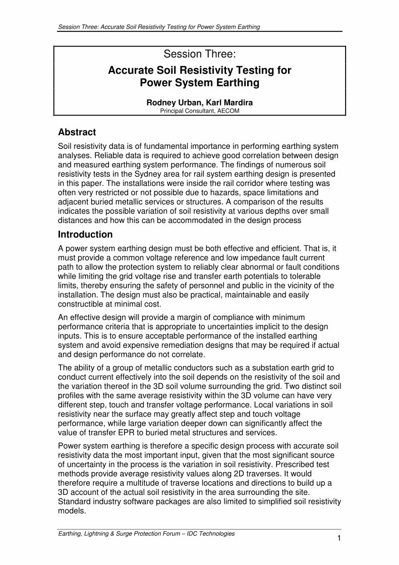
Soil Resistivity Measurement Methods Numerous methods have been developed to determine the resistivity of soil and variations thereof in a specific plane (e.g. vertically). The most accurate of these methods is the four probe method [1] illustrated in Figure 1.

Figure 1: Four electrode soil resistivity test method with equal probe spacing (Wenner)

Current is injected into the soil between using two probes (C1 and C2). The current diverges from the buried surface of the probes into the soil in a spherical pattern. The size of the spherical current expansion within the volume of soil is limited by the distance between the two current probes. Two voltage probes are then inserted into the ground between the two current probes such that all electrodes form a straight traverse. The voltage between the



measurement probes is recorded with a high impedance voltmeter. The ratio of measured voltage to injected current gives the average resistance of the current path through the soil, the apparent resistance. The relationship between the apparent resistance and average soil resistivity is derived from the probe depths and the separation between the probes. If the probes are inserted to a depth less than 5% of the probe spacing and the probe spacings are uniform (i.e. the Wenner method), the relationship simplifies to that included in Figure 1, which is easy to implement in the field during testing. The probe spacing is then increased to an appropriate maximum value to determine the variation of soil resistivity with increased depth.

Figure 2: Four electrode test method with unequal probe spacing (Schlumberger)

It may not be possible to maintain a uniform probe spacing at all sites due to physical barriers or buried obstacles. If these obstacles do not interfere with the soil tests along the traverse, an unequal probe spacing can be used, with the distance between adjacent current and voltage rods varied to suite (i.e. Schlumberger method). The modified relationship between apparent resistance and average soil resistivity is included in Figure 2 for the unequal probe spacing.

The measured soil resistivity test data is then entered into a design software package such as the RESAP module of CDEGS and a simplified single layer or multilayer soil profile derived using iterative curve fitting algorithms.

Soil Resistivity Test Plans A Dial-Before-U-Dig search and Detailed Site Survey are requested at the initiation of the design. The data provided indicates the approximate location and construction type for all buried metal services near the installation site. The data is then scaled and mapped onto satellite images of the area. This allows easy identification of preferred test traverses for the design. An example layout drawing, with test plan indicated, is included in Figure 3.

An understanding of the specific construction methods used by the various services and pipeline utilities is very important when determining the preferred location of test traverses. Construction methods have also changed over time with the advent of new coating technologies. It may therefore be useful, for critical locations, to know the year of construction for a particular pipeline. Fortunately, most new gas, fuel and water pipeline installations will have high quality polyethylene coatings to prevent corrosion. These have excellent insulation properties and will not cause interference to soil resistivity test data unless significantly damaged. Many older cast iron pipelines are direct buried with no insulating coating but are constructed in short sections (typically less than 10m) with insulating rubber joints between adjacent sections. These will



also not significantly affect measurements unless the small probe spacing tests are within a few meters of the pipeline.

Figure 3: Buried services layout example with soil resistivity test plan

Geotechnical data is often available for the installation site as part of the civil and structural designs for the installation. Soil resistivity tests can then be conducted at geotechnical test locations and correlations identified between the soil resistivity and geotechnical test data. The most important features of the geotechnical test data, as concerns soil resistivity modelling is the identified depth of ground water and the main classification of soil types with associated layer thickness. By associating a specific range of soil resistivity value to a distinct soil layer, soil profiles can be constructed at installation locations where accurate soil resistivity testing is not feasible but geotechnical data is available.

Variations in the depth of ground water have a significant effect on the resistivity of certain soils (but not all soils). These effects, if present, are therefore seasonal with soil drying during extended dry periods causing an increase in the resistivity of the first few meters of clayey type soil layers. It is therefore very important that the date of the test, the rainfall on the test day and days leading up to the test are recorded. Rainfall patterns for the area can then be referred to using historical data in order to determine how the derived soil model may vary seasonally. It is important that such variations are accommodated in the earthing system design.

The Electricity Authority of New South Wales Earthing Handbook [2] provides useful data regarding the recorded seasonal variation of soil resistivity at various test sites throughout the Sydney area. Similar references for other areas are equally useful when determining appropriate seasonal variations in soil resistivity for the design process (i.e. to limit input uncertainty).

The length of each test traverse (i.e. the maximum probe spacing) must be appropriate to the depth of the soil which must be interrogated. This is determined by the size of the required earth grid. The basic guideline is that the depth to which the soil is interrogated is typically about that of the maximum



probe spacing. This is however only valid for small to moderate variations in soil resistivity with increasing depth. A soil profile comprising a very high resistivity middle layer just below the surface may require very large probe spacings to get sufficient test current into the lower resistivity bottom layer such that you can accurately determine its value.

At sites where the maximum possible length of a test traverse is restricted, there may still be value in measuring the apparent resistance at short probe spacings at the installation site. Variations at the surface are typically more pronounced due to construction activity and small geological features, while those deeper down typically vary less over smaller distances. Large probe spacing measurements further from the installation site can be used to derive the depth and resistivity of the bottom soil layers while the small probe spacing measurements can be used to derive the actual soil resistivity of the top soil in which the electrodes will be installed. Care must however be exercised in interpreting soil resistivity data from restricted test traverses.

The above mentioned considerations for developing an effective soil resistivity test plan are next discussed with the aid of three case studies. The final test plan and soil test results are presented. Features of the final design that accommodate the assessed uncertainty in the soil resistivity model are also discussed.

Case Study 1 – Using Geotechnical Input Data The first case study involves a number of earth grid designs that formed part of upgrade works along 5km of duplicated track in Western Sydney. These included earthing system designs for a new traction substation, passenger station supply and signalling supply upgrades at two existing stations.

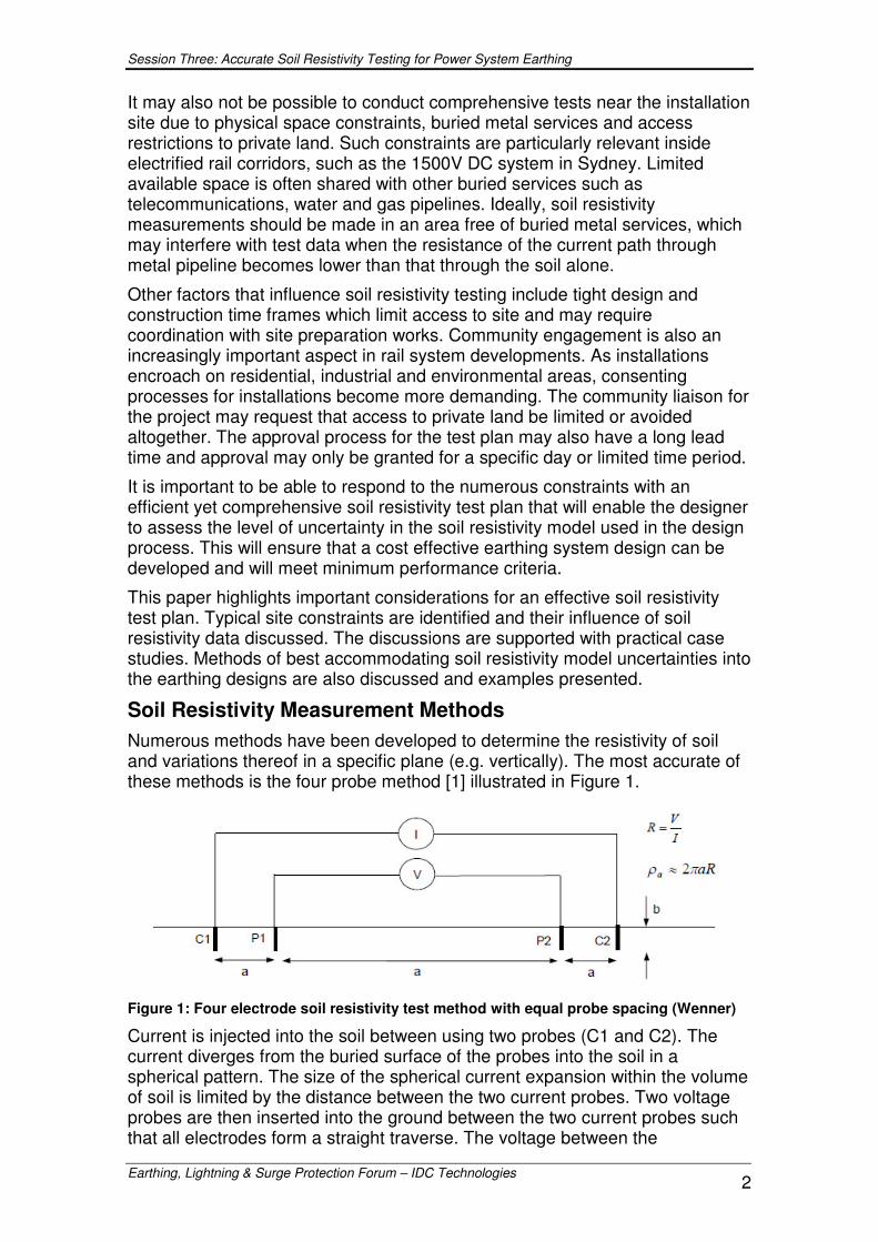
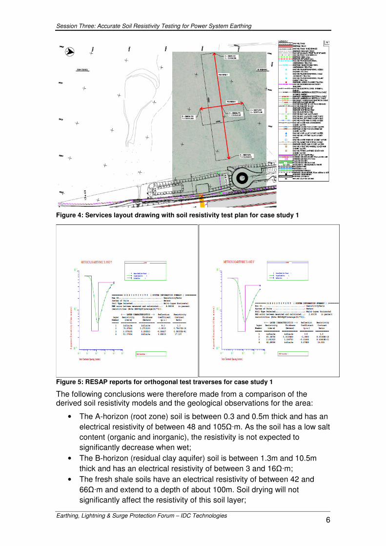
The new passenger station is located on pasture land with no records of buried metal services. The location therefore facilitated a long test traverse centred at the installation site, as well as along a traverse normal to the primary traverse. The test traverse locations are indicated in Figure 4 along with the RESAP modelling reports included in Figure 5.

The soil resistivity profiles derived at various locations along the route are summarized in Table 1. They exhibit a common profile, including an extremely low resistivity middle layer. There were no buried metal services or structures indicated on the layout maps and there was a strong correlation between data measured along the orthogonal test traverses. The feature was however unusual and was identified as having a significant impact on the earthing system designs for the project. Geological references for the region were therefore sought to understand the reason for the observed soil electrical properties and the level of uncertainty associated with variations of it along the route.

Geological observations in [3] noted that the area comprises Wianamatta shales with scattered zones of fracture porosity in the weathered shale allowing saline ground water to rise to the surface, causing surface salting. The source of the salt is windblown aerosols which accumulate in the clay subsoil aquifer. The recorded soil salinity in the area is about 19g/litre which is very high. The reference also noted that the thickness of the aquifer varied from about 1m on hill crests to 12m on valley floors (typically 10m near the midpoint).



Figure 4: Services layout drawing with soil resistivity test plan for case study 1

Figure 5: RESAP reports for orthogonal test traverses for case study 1

The following conclusions were therefore made from a comparison of the derived soil resistivity models and the geological observations for the area:

• The A-horizon (root zone) soil is between 0.3 and 0.5m thick and has an electrical resistivity of between 48 and 105��m. As the soil has a low salt content (organic and inorganic), the resistivity is not expected to significantly decrease when wet;

• The B-horizon (residual clay aquifer) soil is between 1.3m and 10.5m thick and has an electrical resistivity of between 3 and 16��m;

• The fresh shale soils have an electrical resistivity of between 42 and 66��m and extend to a depth of about 100m. Soil drying will not significantly affect the resistivity of this soil layer;



Location GPS Layer Resistivity[�·m] Thickness[m]

Top 105 0.4

Middle 4 4.5 Quakers Hill

Station (test 2)

X = 289277.485 Y = 1266561.495

Bottom 66 �

Top 76 0.3

Middle 3 1.3

Relocated Schofields

Station (test 3 & 4)

X = 288086.276 Y = 1269043.185

Bottom 42 �

Top 49 0.5

Middle 16 10.5 Reycroft (midway) (test 1)

X = 288086.276 Y = 1269043.185

Bottom 48 �

Top 48 0.3

Middle 3 1.3 New Schofields

Substation (test 5)

X = 288086.276 Y = 1269043.185

Bottom 42 �

Table 1: Soil resistivity models along project route

While there had been no rain on the day of the soil tests, there had been significant rainfall in the weeks leading up to the tests. There was therefore a concern, given the nature of the most significant feature of the soil model (i.e. the middle soil aquifer layer), that soil drying may significantly affect the seasonal performance of the earthing systems. All designs therefore considered a 100% increase in resistivity of the middle soil layer. This value was consistent with recorded seasonal variations in an adjacent region, documented in the NSW Earthing Handbook [2]. It was therefore expected to accommodate the assessed level of uncertainty in the input data without resulting in an overly elaborate and expensive earthing system.

The project design phase continued for more than a year. During this time, various grid resistance measurements were conducted on existing installations and additional soil resistivity tests were conducted at specific locations along the route. Tests taken during dry spells indicated no significant change in soil resistivity in the middle soil layer. The design feature included to accommodate soil drying was therefore proven to be conservative.

The final design for the project involved a new earth grid for a pole mount transformer. The installation was adjacent to sensitive signalling equipment and within 10m of a frequented public platform and access footpath at an existing station. The required design criteria were therefore onerous. Furthermore, there was no space available in the congested rail corridor (including direct buried tracer wires associated with the signalling cables) to do meaningful soil resistivity testing. Geotechnical data was however available for test locations adjacent to the relevant pole. This data indicated that the clayey aquifer previously identified was 5m deep and 0.5m below the surface. The soil resistivity model in the area was therefore adjusted (depth and thickness of middle layer) for use in the design.

It was found by CDEGS modelling that it was not possible to accommodate a 100% increase in middle layer resistivity with a reasonable design due to significant public hazards adjacent to the installation. It was therefore decided to ignore soil drying, based on the confidence gained in the accuracy of the soil resistivity models and the expected variation due to soil drying. The design,



which had a minimum 15% margin of compliance, was therefore approved for construction.

An off-frequency current injection test [1] was subsequently conducted to verify the performance of the installed earthing system. The verification test results were within 5% of the calculated design values. It was therefore possible to successfully design the critical earthing system without requiring soil resistivity test data at the actual installation site. Instead, geotechnical data, correlations between geotechnical and electrical resistivity data and a measure of the expected seasonal variations in soil electrical behaviour were used as inputs into the design.

Case Study 2 – Accommodating Probe Spacing Restrictions The next case study involves an 11kV padmount substation earth grid with cable screen bonded UGOH transition pole earth electrode adjacent to a system substation with substantial buried earth grid. Soil resistivity tests were conducted using the Wenner method along a traverse orthogonal to the grid to mitigate the effect of the buried structure on the data. The maximum possible probe spacing along this traverse was 40m. The RESAP modelling report is included in Figure 6 and the derived soil profile is summarized in Table 2.

Figure 6: RESAP report for soil resistivity test traverse for case study 2

Location GPS Layer Resistivity

[�·m] Thickness

[m]

Top 98 1.13

Middle 1 48 2.04

Middle 2 319 10.5 SD17

34° 01’ 41.38’’ S 151° 03’ 33.87’’ E

Bottom 58 �

Table 2: Soil resistivity model for the UGOH pole earth electrode design for case study 2

The most significant feature of the derived soil profile is a thick, high-resistivity middle soil layer. Geotechnical investigations in the area confirmed the presence of a substantial sandstone shelf a few meters below the surface. In order to achieve a suitably low resistivity and limit the earth grid voltage rise to



an acceptable level, an 18m vertical earth electrode was used in the design to prevent interference to sensitive signalling installations adjacent to the pole. The 40m probe spacing limit was considered adequate for this design. To limit excessive transfer voltage to nearby metal pipelines and signalling installations, the vertical electrode was insulated from the low-resistivity top soil layers.

The critical soil parameters, as regards the performance of the earth grid, are the resistivity and depth of the bottom soil layer in which the electrode is buried. The traverse centre point was located at the pole base and far from any buried metal services or structures. The derived soil profile was therefore considered accurate for the electrode design and the design implemented.

A verification test using the Fall-of-Potential method [1] was undertaken on the installed pole earth electrode. This was done to verify the EPR risk assessment which was based on the design performance calculations. The design grid resistance for the pole earth electrode was 21�. The measured earth resistance of the installed electrode was 10�, which is substantially lower than the design value. A review of the modelling error considered that if the depth of the middle/bottom layer interface was incorrectly modelled, the earth resistance would have either remained almost unchanged (interface higher than expected) or increased (interface lower than expected). Since the installed value is lower than the design value, it was concluded that the resistivity of the bottom soil layer was incorrect in the soil model used for the design.

A review of the design process concluded that the calculation error was due to inadequate resistivity data between 10m and 30m probe spacings along the test traverse. The average resistivity at small probe spacings is about 100�m, that of the top soil layer. It decreases slightly before the probe spacing exceeds the depth of the top/middle layer interface. The much higher resistivity middle layer steadily increases the average resistivity as a weighted average of the two layers (first inflection point) until the probe spacing is much larger than the thickness of the top soil layer and the average resistivity value flattens off to that of the middle layer resistivity. When the probe spacing exceeds the depth of the middle/bottom layer interface, the average resistivity begins to steadily decrease (second inflection point). The calculated value of the bottom soil layer is taken from the gradient of the fitted curve after the second inflection point. It is important to note that there is only a single data point on this section of the curve. The bottom layer resistivity is therefore determined by the gradient between the second-last and last measured data points and its accuracy depends on the assumption that the second-last point is the exact point of inflection. Measurements were made at probe spacings of 0.5m, 1m, 2m, 3m, 4m ,6m, 8m, 10m, 15m, 20m and 40m as specified in the generic test plan.

An accurate soil profile could have been derived from the maximum 120m traverse but required refined probe spacings between 10m and 30m to determine the correct location of the inflection point and therefore the gradient of the final curve section. The following conclusions were made:

• The selected test traverse location and extent was appropriate for the soil structure and design;

• It was correct to follow the generic test plan with set probe spacings initially;



• The data points should have been plotted on graph paper during the test;

• The critical design parameters should have been identified in light of the observed hazards and basic soil structure;

• The dependence of the bottom layer soil resistivity on the observed inflection point of the plotted curve and the lack of data points on the final curve section should have been flagged as inadequate for the purposes of the design;

• Refined probe spacings between 10m and 30m should have been used during the tests.

Case Study 3 – Influence of Buried services The final case study involved the design of a padmount substation in Western Sydney. The services layout and test plan for the soil resistivity measurements are indicated in Figure 7. A second traverse, at 45° to the first was chosen to determine the possible interference to the data caused by the water pipeline adjacent to the first test traverse. The test locations are not ideal due to space limitation and adjacent buried metallic services. Traverse 1 runs parallel to the metal pipeline. The separation distance is about 5m.

Figure 7: Services layout drawing with soil resistivity test plan for case study 3

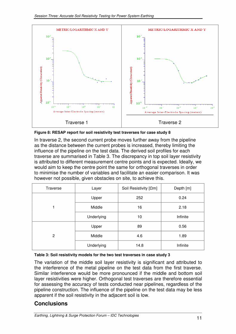
The RESAP modelling reports are included in Figure 8 for both test traverses. The ‘best-fit’ soil resistivity models are both three layer soil profiles. The resistivity curve on traverse 1 which runs parallel to the metallic pipe shows a degree of interference with the test data after the 1m probe spacing. This is because the distance between voltage probes and current probes is increasing while the distance between the metallic pipe and the current probe remains constant (5m).The resistance of the current path between the current probes through the metal pipeline becomes increasingly lower than the current path through the soil. This causes the influence of the metallic pipe to become larger with increased probe spacing. This can be seen at the test results after 1m probe spacing.

Legend

Metallic Water Services

Traverse

Proposed Substation

1

2



Traverse 1

Traverse 2

Figure 8: RESAP report for soil resistivity test traverses for case study 8

In traverse 2, the second current probe moves further away from the pipeline as the distance between the current probes is increased, thereby limiting the influence of the pipeline on the test data. The derived soil profiles for each traverse are summarised in Table 3. The discrepancy in top soil layer resistivity is attributed to different measurement centre points and is expected. Ideally, we would aim to keep the centre point the same for orthogonal traverses in order to minimise the number of variables and facilitate an easier comparison. It was however not possible, given obstacles on site, to achieve this.

Traverse Layer Soil Resistivity [�m] Depth [m]

Upper 252 0.24

Middle 16 2.18 1

Underlying 10 Infinite

Upper 89 0.56

Middle 4.6 1.89 2

Underlying 14.8 Infinite

Table 3: Soil resistivity models for the two test traverses in case study 3

The variation of the middle soil layer resistivity is significant and attributed to the interference of the metal pipeline on the test data from the first traverse. Similar interference would be more pronounced if the middle and bottom soil layer resistivities were higher. Orthogonal test traverses are therefore essential for assessing the accuracy of tests conducted near pipelines, regardless of the pipeline construction. The influence of the pipeline on the test data may be less apparent if the soil resistivity in the adjacent soil is low.

Conclusions



• The most significant sources of uncertainty in the earthing system design process are the variations in the resistivity of the soil surrounding the earthing system and seasonal variations thereof.

• An effective earthing system design must accommodate the level of uncertainty in the design inputs in a practical, constructible and maintainable design at minimal cost. This requires an accurate assessment of the uncertainties.

• Buried services, physical obstacles and project related access limitations constrain the accuracy of soil resistivity measurement data.

• Service layout maps, geotechnical data and published meteorological data can be used to assess the optimal soil model and uncertainty thereof for the design process.

• Soil resistivity test data should be plotted during measurements in order to identify possible inaccuracies that can be reduced by further testing at/near the test site.

References [1] IEEE 81, Guide for Measuring Earth Resistivity, Ground Impedance and

Surface Potentials of a Ground system, 1983.

[2] Electricity Authority of New South Wales, Earthing Handbook, Sydney, 1975.

[3] G. McNally, “Shale, Salinity and Groundwater in Western Sydney”, Australian Geomechanics Vol. 39 No. 3, September 2004.

session 3 rodney urban paper final and lightning/soil resistivity testing... · earthing, lightning...

Documents