sergei grudinin, maria garkavenko, andrei kazennov

HAL Id: hal-01516719https://hal.inria.fr/hal-01516719

Submitted on 25 Jul 2017

HAL is a multi-disciplinary open accessarchive for the deposit and dissemination of sci-entific research documents, whether they are pub-lished or not. The documents may come fromteaching and research institutions in France orabroad, or from public or private research centers.

L’archive ouverte pluridisciplinaire HAL, estdestinée au dépôt et à la diffusion de documentsscientifiques de niveau recherche, publiés ou non,émanant des établissements d’enseignement et derecherche français ou étrangers, des laboratoirespublics ou privés.

Copyright

Pepsi-SAXS : an adaptive method for rapid and accuratecomputation of small-angle X-ray scattering profiles

Sergei Grudinin, Maria Garkavenko, Andrei Kazennov

To cite this version:Sergei Grudinin, Maria Garkavenko, Andrei Kazennov. Pepsi-SAXS : an adaptive method for rapidand accurate computation of small-angle X-ray scattering profiles. Acta Crystallographica SectionD: Biological Crystallography, International Union of Crystallography, 2017, D73, pp.449 - 464.�10.1107/S2059798317005745�. �hal-01516719�

https://hal.inria.fr/hal-01516719

https://hal.archives-ouvertes.fr

electronic reprint

ISSN: 2059-7983

journals.iucr.org/d

Pepsi-SAXS: an adaptive method for rapid and accuratecomputation of small-angle X-ray scattering profiles

Sergei Grudinin, Maria Garkavenko and Andrei Kazennov

Acta Cryst. (2017). D73, 449–464

IUCr JournalsCRYSTALLOGRAPHY JOURNALS ONLINE

Copyright c⃝ International Union of Crystallography

Author(s) of this paper may load this reprint on their own web site or institutional repository provided thatthis cover page is retained. Republication of this article or its storage in electronic databases other than asspecified above is not permitted without prior permission in writing from the IUCr.

For further information see http://journals.iucr.org/services/authorrights.html

Acta Cryst. (2017). D73, 449–464 Grudinin et al. · Pepsi-SAXS

http://journals.iucr.org/d/

https://doi.org/10.1107/S2059798317005745

http://journals.iucr.org/services/authorrights.html

http://crossmark.crossref.org/dialog/?doi=10.1107/S2059798317005745&domain=pdf&date_stamp=2017-04-27

research papers

Acta Cryst. (2017). D73, 449–464 https://doi.org/10.1107/S2059798317005745 449

Received 1 July 2015

Accepted 15 April 2017

Edited by S. Wakatsuki, Stanford

University, USA

Keywords: Pepsi-SAXS; small-angle scattering;

multipole expansion.

Supporting information: this article has

supporting information at journals.iucr.org/d

Pepsi-SAXS: an adaptive method for rapid andaccurate computation of small-angle X-rayscattering profiles

Sergei Grudinin,a,b,c* Maria Garkavenkod and Andrei Kazennovd

aUniversite Grenoble Alpes, LJK, F-38000 Grenoble, France, bCNRS, LJK, F-38000 Grenoble, France, cInria, France, anddMoscow Institute of Physics and Technology, Dolgoprudniy, Russian Federation. *Correspondence e-mail:

[email protected]

A new method called Pepsi-SAXS is presented that calculates small-angle X-rayscattering profiles from atomistic models. The method is based on the multipoleexpansion scheme and is significantly faster compared with other testedmethods. In particular, using the Nyquist–Shannon–Kotelnikov samplingtheorem, the multipole expansion order is adapted to the size of the modeland the resolution of the experimental data. It is argued that by using theadaptive expansion order, this method has the same quadratic dependence onthe number of atoms in the model as the Debye-based approach, but with amuch smaller prefactor in the computational complexity. The method has beensystematically validated on a large set of over 50 models collected from theBioIsis and SASBDB databases. Using a laptop, it was demonstrated that Pepsi-SAXS is about seven, 29 and 36 times faster compared with CRYSOL, FoXS andthe three-dimensional Zernike method in SAStbx, respectively, when tested ondata from the BioIsis database, and is about five, 21 and 25 times fastercompared with CRYSOL, FoXS and SAStbx, respectively, when tested on datafrom SASBDB. On average, Pepsi-SAXS demonstrates comparable accuracy interms of !2 to CRYSOL and FoXS when tested on BioIsis and SASBDBprofiles. Together with a small allowed variation of adjustable parameters, thisdemonstrates the effectiveness of the method. Pepsi-SAXS is available at http://team.inria.fr/nano-d/software/pepsi-saxs.

1. Introduction

Small-angle scattering is one of the fundamental techniquesfor the structural study of biological systems. Small-angleX-ray scattering (SAXS) is a type of small-angle scattering inwhich X-rays are scattered elastically from the sample and arethen collected at very small angles. Compared with otherstructure-determination methods, SAXS experiments are verysimple conceptually, and thanks to advances in instrumenta-tion (Spilotros & Svergun, 2014), the SAXS technique,particularly solution-state SAXS, has become very popular inrecent years as a complement to other methods in structuralbiology (Graewert & Svergun, 2013; Putnam et al., 2007).SAXS also allows some of the restrictions of other experi-mental techniques to be overcome; for example, it is applic-able to systems of all sizes, it allows the study of particles insolution, it is very fast and it destroys the sample onlymarginally. On the downside, SAXS can only determine thedistance distribution function of the electron density at aresolution above nanometres; however, it can distinguishconformations of a protein at subnanometre resolution(Zheng & Tekpinar, 2011).

Over the years, a number of computational tools have beendeveloped for the analysis of solution-state SAXS curves,

ISSN 2059-7983

# 2017 International Union of Crystallography

electronic reprint

calculation of theoretical profiles and low-resolution recon-struction of model shapes. The most prominent of them is theATSAS package developed at EMBL Hamburg (Petoukhov etal., 2012). To test a structural hypothesis or to construct amodel system based on a SAXS experiment, an accurate andrapid calculation of a model SAXS profile is required. Therunning time of a computational method depends, amongother things, on the number of atoms in the model N and thenumber of points in the scattering curve M. Tools that directlyuse the Debye equation have a cost of O(N2), whereas toolsthat use a linear approximation to the scattering equationhave a cost of O(N). Generally speaking, the same type ofcalculation should be repeated for each point in the scatteringcurve, which determines the worst-case performance asO(N2M). Keeping in mind that the typical values of M and Nare several thousand, this running time usually prohibits theperformance of any kind of multiple model assessment. Thus,much effort has been devoted in recent years to reducing therunning time of SAXS computational tools without degradingthe quality of their approximations. Below, we give a briefoverview of the most notable computational methods for thecalculation of theoretical SAXS profiles given an atomicmodel as input. A deeper discussion of different computa-tional techniques can be found elsewhere (Rambo & Tainer,2013b).

The most popular method is the CRYSOL program devel-oped by Svergun and coworkers (Svergun et al., 1995). Thismethod uses the theory of multipole expansions of scatteringintensity initially developed by Stuhrmann (Stuhrmann,1970b). The running time of the initial implementation of themethod had a linear dependence on both the number of atomsin the molecule N and the number of points in the scatteringcurve M as O(NM). A more recent version of the program,however, maps experimental scattering intensities and asso-ciated errors onto a sparser grid (Petoukhov et al., 2012), thusreducing the computational cost to O(N + M). The method isgenerally very fast, but has the major disadvantage of asimplistic representation of the hydration shell of the sampleusing a two-dimensional angular function (Stuhrmann, 1970a).The SASSIM method is very similar to CRYSOL, but thehydration shell is defined in terms of spherical harmonics andis calculated using a Lebedev grid (Merzel & Smith, 2002).

Another popular program, FoXS, uses a linear approx-imation to the Debye scattering equation, which decouples thedependency of the running time on the number of atoms N ina model and the number of points in the scattering curve M asO(N2 + MN) (Schneidman-Duhovny et al., 2010, 2013). Whencreated, the program was notably faster compared with theinitial implementation of CRYSOL when tested on experi-mental curves with several thousands of points. However, thelater development of CRYSOL, as we demonstrate below,outperforms FoXS for nearly all test cases.

A logical extension of the multipole expansion method is acomputational scheme that uses three-dimensional Zernikepolynomials for the representation of the electron density(Liu, Poon et al., 2012). Here, the angular dependence of thescattering amplitudes on the scattering vector is described,

similarly to that in CRYSOL, using spherical harmonics, butthe radial dependence is expanded using a set of orthogonalfunctions. The computational complexity of this method isO(N + M); however, the hidden time-limiting step is thecomputation of the three-dimensional Zernike moments. Inorder to calculate them, atomic models are mapped onto athree-dimensional grid, the size of which can be adjustedaccording to the resolution of the data.

Recently, some other linear scaling schemes have beenproposed. The golden-ratio scheme described by Watson &Curtis (2013) uses Euler’s formula to compute the rotationallyaveraged scattering intensity I(q) by evaluating I(q) in severalscattering directions using the exact expression for I(q) at agiven wavevector q. The orientations of the q vectors aretaken from a quasi-uniform spherical grid generated by thegolden ratio. The hierarchical algorithm for fast summation ofthe Debye equation by Gumerov et al. (2012) is similar to thefast multipole method (FMM) and is based on a hierarchicalspatial decomposition of electron density using local harmonicexpansions and translation operators for these expansions. Itscomputational cost is O(N logN).

Some efforts have been made to obtain a more precisedescription of solvation. The AXES method uses explicitwater molecules equilibrated in a water box using molecular-dynamics (MD) simulations to accurately model the scatteringamplitudes of the surface and displaced solvent (Grishaev etal., 2010). Another method calculates hydration-shell inten-sities from MD trajectories of water molecules around a fixedprotein (Park et al., 2009). The AquaSAXS method models thenon-uniform hydration shell of a protein by taking advantageof recently developed methods that compute the solventdistribution around a given solute on a three-dimensional grid,such as the Poisson–Boltzmann–Langevin formalism or thethree-dimensional reference interaction-site model (Poitevinet al., 2011).

Finally, to increase the speed of calculations, several coarse-grained schemes have been proposed. For example, one recentmethod is based on the Debye formula and a set of scatteringform factors for dummy-atom representations of amino acids(Stovgaard et al., 2010). The Fast-SAXS-pro (Yang et al., 2009)algorithm uses the Debye-based approach and coarse-grainedresidue-level and nucleotide-level structure factors. Themethod explicitly takes into account the nonhomogeneousdistribution within the hydration layer by assigning a differentscaling factor for dummy water molecules according to theirproximity to protein and DNA/RNA. Finally, the method ofZheng & Tekpinar (2011) uses a one-bead-per-residue coarse-grained protein representation coupled with the elasticnetwork model. The hydration shell is modelled implicitly bycombining each residue and its nearby implicit water mole-cules into a composite representation.

Here, we present Pepsi-SAXS (where ‘Pepsi’ stands for‘polynomial expansions of protein structures and inter-actions’), a new implementation of the multipole-basedscheme proposed by Stuhrmann (Stuhrmann, 1970b). Overall,our method is significantly faster compared with CRYSOL,FoXS and the three-dimensional Zernike implementation in

research papers

450 Grudinin et al. ! Pepsi-SAXS Acta Cryst. (2017). D73, 449–464

electronic reprint

the SAStbx package (Liu, Hexemer et al., 2012), as wedemonstrate below using a large number of test cases. Ourmethod has the following features. Firstly, we use a very fastmodel for computation of the hydration shell based on auniform grid of points. Secondly, we use the adaptive orderof the multipole expansion. More precisely, according to theNyquist–Shannon–Kotelnikov sampling theorem (Marks,2008), we determine the required expansion order using theradius of gyration of the model’s hydration shell and the valueof the maximum scattering vector qmax. Thirdly, we representthe scattering intensity curve using a cubic spline interpola-tion, which allows us to significantly speed up the running timeof our method. Finally, we introduce partial scattering inten-sities to rapidly fit the theoretical curve to the experimentalcurve using an exhaustive search in two adjustable parameters.We should also mention that we pay particular attention whenderiving parameters for the form factors, especially those forcharged and resonance groups.

2. Theory

Here, we follow the scattering theory initially described byH. B. Stuhrmann and later revised by D. Svergun (Stuhrmann,1970b; Svergun, 1991; Svergun et al., 1995). The sphericallyaveraged scattering intensity I(q) from a single moleculeimmersed in a solvent with bulk scattering density " can bewritten as

IðqÞ ¼ hjAaðqÞ % "AcðqÞ þ #"AbðqÞj2i!; ð1Þ

where Aa(q) is the scattering amplitude from the molecule invacuum, Ac(q) is the scattering amplitude from the excludedvolume and Ab(q) is that from the hydration shell, which isassumed to have a scattering density that differs from the bulkvalue by #" (Svergun et al., 1995). We should mention thatthroughout the paper we use the following definition of thescattering vector q: q = 4$sin%/&, where 2% is the scatteringangle and & is the wavelength. Owing to the spherical aver-aging of the intensity, it is very convenient to introduce themultipole expansion of the scattering intensities and ampli-tudes in the spherical coordinates system (Stuhrmann, 1970b).Using this expansion up to the maximum expansion order L,we can rewrite the intensity as

IðqÞ ’PL

l¼0

Pl

m¼%l

jAlmðqÞ % "ClmðqÞ þ #"BlmðqÞj2; ð2Þ

where Alm(q), Blm(q) and Clm(q) are the expansion coeffi-cients of the amplitudes Aa(q), Ab(q) and Ac(q), respectively(Svergun et al., 1995). Given the atomic coordinates of amolecule consisting of N atoms expressed in the sphericalcoordinate system ri ' (ri, !i) and the corresponding formfactors fi(q), we can write the vacuum scattering-amplitudeexpansion coefficients as

AlmðqÞ ¼ 4$il PN

i¼1

fiðqÞjlðqriÞY(lmð!iÞ; ð3Þ

where jl(qri) are the spherical Bessel functions and Y(lmð!iÞ are

the complex-conjugated spherical harmonics. Similarly, giventhe coordinates of the hydration shell of the molecule sampledat Nhs points, its expansion coefficients can be written as

BlmðqÞ ¼ 4$ilhðqÞPNhs

i¼1

jlðqriÞY(lmð!iÞ; ð4Þ

where h(q) is the form factor of a water molecule scaled withthe ratio of the bulk water density to the density of thesampling points in the hydration shell. Finally, the excludedvolume contribution can be written as

ClmðqÞ ¼ 4$ilPN

i¼1

giðqÞjlðqriÞY(lmð!iÞ; ð5Þ

where gi(q) are the form factors of the dummy atoms centredat the positions of molecular atoms ri.

2.1. Form factors and unified atomic groups

Computation of the expansion coefficients Alm(q), Blm(q)and Clm(q) requires knowledge of the form factors fi(q), gi(q)and hi(q). For the calculation of form factors for the individualatoms, we use the five-Gaussian approximation with coeffi-cients taken from Waasmaier & Kirfel (1995):

f ðqÞ ¼ c þP5

i¼1

ai expð%biq2Þ: ð6Þ

However, structural databases such as the Protein Data Bank(PDB; Berman et al., 2000) typically provide the coordinatesof only non-H atoms. Therefore, it is useful to introduceunified atomic groups with the positions located at the centresof the nuclei of heavy atoms and the corresponding scatteringparameters computed for the heavy atoms with covalentlybonded H atoms. For example, the form factor for such agroup fCHn

, with n H atoms attached to a C heavy atom, can becomputed using the Debye equation as follows,

fCHnðqÞ2 ¼ fCðqÞ

2 þ n2fHðqÞ2 þ 2nfHðqÞ

sinðqrHÞqrH

; ð7Þ

where fC and fH are the atomic form factors for C and H atomsgiven by the five-Gaussian approximation (6), and rH is thedistance between C and H atoms. The distances rH betweenthe heavy atom and H atoms in various atomic groups typicalfor biological molecules are taken from Allen et al. (2004)and are listed in Table 1. We should note that a simpler

research papers

Acta Cryst. (2017). D73, 449–464 Grudinin et al. ! Pepsi-SAXS 451

Table 1Crystallographic distances between heavy atoms and their attached Hatoms (Allen et al., 2004).

Various atomic groups typical for biological molecules are listed.

Atomic group Distance to the H atom (A)

C(sp3)—H 1.099C(sp3)—H2 1.092C(sp3)—H3 1.059C(sp2)—H 1.077C(arom)—H 1.083O(alc)—H 0.967O(acid)—H 1.015N—H 1.009N+—H 1.033

electronic reprint

approximation holds for practical values of the scatteringvector q (Harker, 1953),

fCHnðqÞ ¼ fCðqÞ þ nfHðqÞ

sinðqrHÞqrH

; ð8Þ

which can also be derived from spherical averaging of thescattering amplitudes instead of the scattering intensities.

We explicitly introduced individual form factors for thecharged groups carboxylate, phosphate, guanidine and ammo-nium. Form factors for NH+, NH2

+ and NH3+ from guanidine

and ammonium groups were approximated according to themodel of the electron distribution in the ammonium ion(Banyard & March, 1961). More specifically, we modelled thecentral spherical charge cloud with six electrons around the Nnucleus with unperturbed H electron distributions centred noton the protons but inwards along the N—H bonds at 0.76 ofthe N—H separation distance. We also paid particular atten-tion to the resonance forms of the charged groups carboxylate,phosphate and guanidine. More precisely, we modelled theform factors of the resonance groups as a linear combinationof the nonresonance form factors. Given the analytic form ofthe atomic form factors for unified atomic groups (8), wecomputed their five-Gaussian approximations, which weretabulated for later use. Table 2 lists the obtained coefficients.

2.2. Form factors for dummy atoms

Following Fraser et al. (1978), we express the form factorsof the dummy atoms through the observed displaced solventvolumes Vi as

giðqÞ ¼ Vi expð%$q2V2=3i Þ: ð9Þ

Following Svergun et al. (1995), we introduce the effectiveatomic radius r0, an adjustable parameter that scales theobserved displaced solvent volumes according to

Viðr0Þ ¼4

3$r3

i

r30

r3m

; ð10Þ

where ri are the tabulated actual values of atomic group radiiand rm are the actual average radii of atomic groups. Changingthe adjustable parameter to #r ' r0 % rm, we can expand theprevious expression to the first order in #r using the Maclaurinseries as

giðq; #rÞ ¼ Vi expð%$q2V2=3i Þ 1 þ #r

rm

ð3 % 2$q2V2=3i Þ

! "

þ Oð#r2Þ: ð11Þ

This equation can be further simplified to the form ofexpressions (12) and (13) from Svergun et al. (1995) as

giðq; #rÞ ¼ Vi expð%$q2V2=3i Þ 1 þ #r

rm

3 % 4$

3

# $2=3

2$q2r2m

" #( )

þ Oð#r2Þ; ð12Þ

with the term independent of #r being the reference dummy-atoms form factor gi(q) and the term in the curly bracketsbeing the adjustable overall expansion factor G(q, #r). We caneven simplify the second term further, dropping the depen-dence on q. Using the last expression, the excluded volume

research papers


Table 2Coefficients of the five-Gaussian approximation as given by (6) for different unified atomic groups.

The approximation was calculated according to (8) at 950 points for values of q in the range (0, 0.95) using the nonlinear least-squares Levenberg–Marquardtalgorithm. The standard deviations of the approximations do not exceed 10%4 for all of the form factors. The unified atomic groups include sp2, sp3 and aromatic Catoms with one or several H atoms attached, carboxylate or phosphate resonance O atoms, O atoms and S atoms with an attached H atom, neutral and charged Natoms with one or several H atoms attached, and the N atoms of the guanidine group.

C(sp3)—H C(sp3)—H2 C(sp3)—H3 C(sp2)—H C(arom)—H O(alc)—H O(acid)—H O(resonance)

a1 2.909530 3.275723 3.681341 2.909457 2.168070 0.456221 3.213280 0.688944a2 0.485267 0.870037 1.228691 0.484873 1.275811 3.219608 0.463019 2.929687a3 1.516151 1.534606 1.549320 1.515916 1.561096 0.812773 0.815724 0.416472a4 0.206905 0.395078 0.574033 0.207091 0.742395 2.666928 2.664450 2.606983a5 1.541626 1.544562 1.554377 1.541518 %6.151144 1.380927 1.384266 1.319232b1 13.933084 13.408502 13.026207 13.934162 12.642907 21.503498 13.383078 29.319200b2 23.221524 23.785175 24.131974 23.229153 18.420069 13.397134 21.362223 6.572228b3 41.990403 41.922444 41.869426 41.991425 41.768517 34.547137 34.531415 64.951658b4 4.974183 5.019072 4.984373 4.983276 1.535360 5.826620 5.823549 16.267799b5 0.679266 0.724439 0.765769 0.679898 %0.045937 0.412902 0.410805 0.455640c 0.337670 0.377096 0.409294 0.338296 7.400917 0.463202 0.458919 0.537548

N—H N—H2 N—H+ N—H2+ N—H3

+ (N—H) (guanine) (N—H2) (guanine) S—H

a1 1.650531 1.904157 1.426540 3.823896 1.882162 3.630164 1.792216 0.570042a2 0.429639 1.942536 0.426903 0.531490 1.933200 0.228310 0.724464 6.337416a3 2.144736 2.435585 1.878894 1.713620 2.465843 1.869734 2.347044 1.641643a4 1.851894 0.730512 1.608251 0.322552 0.927311 0.170550 1.903020 5.398549a5 1.408921 1.379728 1.200216 1.287502 1.190889 1.440894 1.313042 1.527982b1 10.603730 10.803702 10.652268 10.305028 10.975157 10.267139 10.830060 11.447986b2 6.987283 10.792421 7.017651 25.631593 10.956008 25.118086 6.846763 1.197657b3 29.939901 29.610479 29.878525 30.215026 29.208572 30.241288 29.579607 55.401032b4 10.573859 6.847755 10.619493 3.576178 6.663555 3.412776 10.800018 22.420955b5 0.611678 0.709687 0.631765 0.506824 0.843650 0.486644 0.720448 2.356552c 0.510589 0.603738 0.456024 0.317728 0.597322 0.323504 0.583312 1.523944

electronic reprint

amplitudes Clm(q, #r) can be adjusted through the referencevalues Clm(q) as

Clmðq; #rÞ ¼ ClmðqÞGðq; #rÞ; ð13Þ

where the reference amplitudes Clm(q) are computed onlyonce using the reference dummy-atoms form factors gi(q). Tocompute the excluded volumes and radii of the unified atomicgroups, we used the parameters provided in Svergun et al.(1995).

2.3. Hydration shell

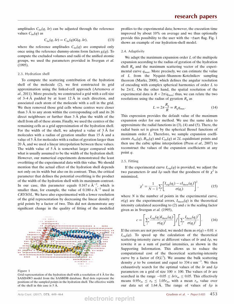
To compute the scattering contribution of the hydrationshell of the molecule (2), we first constructed its gridapproximation using the linked-cell approach (Artemova etal., 2011). More precisely, we constructed a grid with a cell sizeof 3–4 A padded by at least 12 A in each direction, andassociated each atom of the molecule with a cell in the grid.We then removed those grid cells whose centres were closerthan 3 A to any atom within the corresponding cell and its 26direct neighbours or further than 3 A plus the width of theshell from all of these atoms. Finally, we used the centres of theremaining cells as a grid approximation of the hydration shell.For the width of the shell, we adopted a value of 3 A formolecules with a radius of gyration smaller than 15 A and avalue of 5 A for molecules with a radius of gyration larger than20 A, and we used a linear interpolation between these values.The width value of 5 A is somewhat larger compared withwhat is usually assumed to be the width of the hydration shell.However, our numerical experiments demonstrated the leastoverfitting of the experimental data with this value. We shouldmention that the actual effect of the hydration shell dependsnot only on its width but also on its contrast. Thus, the criticalparameter that defines the potential overfitting is the productof the width of the hydration shell with its maximum contrast.In our case, this parameter equals 0.167 e A%2, which issmaller than, for example, the value of 0.180 e A%2 used inCRYSOL. We have also experimented with a lower resolutionof the grid representation by decreasing the linear density ofgrid points by a factor of two. This did not demonstrate anysignificant change in the quality of fitting of the modelled

profiles to the experimental data; however, the execution timeimproved by about 10% on average and we thus optionallyprovide this possibility to the user with the -fast flag. Fig. 1shows an example of our hydration-shell model.

2.4. Adaptivity

We adapt the maximum expansion order L of the multipoleexpansion according to the radius of gyration of the hydrationshell Rg and the maximum scattering vector of the experi-mental curve qmax. More precisely, we can estimate the valueof L from the Nyquist–Shannon–Kotelnikov samplingtheorem (Marks, 2008), which defines the angular resolutionof encoding with complex spherical harmonics of order L tobe 2$/L. On the other hand, the spatial resolution of theexperimental data is R = 2$/qmax; thus, we can relate the tworesolutions using the radius of gyration Rg as

L ¼ 2$Rg

R¼ Rgqmax: ð14Þ

This expression provides the default value of the maximumexpansion order for our method. We use the same idea toapproximate the radial functions in (3), (4) and (5). There, theradial basis set is given by the spherical Bessel functions ofmaximum order L. Therefore, we sample expansion coeffi-cients Alm(q), Blm(q) and Clm(q) at 2L equidistant points andthen use the cubic spline interpolation (Press et al., 2007) toreconstruct the values of the expansion coefficients at anypoint q.

2.5. Fitting

If the experimental curve Iexp(q) is provided, we adjust thetwo parameters #r and #" such that the goodness of fit !2 isminimized,

!2 ¼ 1

N % 1

Pj

IexpðqjÞ % cItheorðqjÞ'ðqjÞ

! "2

; ð15Þ

where N is the number of points in the experimental curve,'(q) are the experimental errors, Itheor(q) is the theoreticalintensity calculated according to (2) and c is the scaling factorgiven as in Svergun et al. (1995),

c ¼P

j

IexpðqjÞItheorðqjÞ'ðqjÞ

2

" #% P

j

ItheorðqjÞ2

'ðqjÞ2

" #

: ð16Þ

If the errors are not provided, we model them as '(q) = 0.01 )Iexp(q). To speed up the calculation of the theoreticalscattering-intensity curve at different values of #r and #", werewrite it as a sum of partial intensities, as shown in theSupporting Information. This allows us to reduce thecomputational cost of the theoretical scattering-intensitycurve by a factor of O(L2). We assume the bulk scatteringdensity " to be constant and equal to 334 e nm%3. We thenexhaustively search for the optimal values of the #r and #"parameters on a grid of size 100 ) 100. The values of #r aresearched in the range %0.05 * #r/rm * 0.05. This effectivelymeans 0.95rm * r0 * 1.05rm, with a mean rm value overour data set of 1.64 A. The range of values of #" is

research papers


Figure 1Grid representation of the hydration shell with a resolution of 4 A for theSASDAW3 model from the SASBDB database. Red dots represent thepositions of the sampled points in the hydration shell. The effective widthof the shell in this case is 5 A.

electronic reprint

0 * #" * 33.4 e nm%3. We should note that upon request fromthe user we allow the contrast of the hydration shell #" to beslightly negative up to %15 e nm%3. Indeed, as has beendemonstrated by X-ray diffraction, neutron and, morerecently, X-ray reflectivity studies of water–hydrophobicinterfaces, there is an unambiguous and distinguishabledensity-depleted interfacial region near hydrophobic inter-faces (Iiyama et al., 1995; Mezger et al., 2011; Chattopadhyay etal., 2010; Uysal et al., 2013). At these interfaces, the waterdensity drops below the bulk value. There is, however, acertain controversy about the width and the density of thisdepletion region (Uysal et al., 2013). We should admit thatprotein surfaces are never fully hydrophobic. Nonetheless, weallow negative #" values upon request from the user. Below,we report the results for the two cases. We should also notethat some experimental measurements have a systematic errorin the determination of the intensity values. To account for thiserror, we can optionally introduce the offset constant ( andrewrite the goodness of fit as shown in the Supporting Infor-mation.

2.6. Benchmarks

We tested our methods using two benchmarks constructedfrom structural models with corresponding experimental

SAXS profiles. We collected experimental data from two largedatabases dedicated to the study of biological molecules usingSAXS experiments. The first database is BioIsis, which wasdesigned by Dr Robert P. Rambo at the Lawrence BerkeleyNational Laboratory (Hura et al., 2009). It currently contains99 SAXS scattering profiles of biological molecules and theircomplexes with both known and unknown structure. The firstentry in BioIsis is dated 2009. The second database is the SmallAngle Scattering Biological Data Bank (SASBDB), poweredby the Biological Small Angle Scattering Group at EuropeanMolecular Biology Laboratory Hamburg Outstation (Valen-tini et al., 2015). This database contains 125 scattering profiles.The first data for SASBDB were collected in 1998. For ourtests, we collected all of the experimental scattering profilesfrom the two databases that had corresponding atomic models.Overall, we use 28 entries from BioIsis and 23 entries fromSASBDB. The models from BioIsis range from 424 to 23 149atoms, with an average of 6676 atoms. The models fromSASBDB range from 602 to 25 761 atoms, with an average of6443 atoms.

2.7. Details of implementation

The presented method was implemented using the C++programming language and compiled with the gcc-4.8

research papers


Table 3Comparison of four methods, CRYSOL, FoXS, SAStbx (using the three-dimensional Zernike technique and data-reduction option) and Pepsi-SAXS,when fitting modelled intensity profiles to experimental data collected from the BioIsis database.

For each method, we provide the value of ! and the running time measured in seconds for each of the scattering profiles. We also list the number of atoms in themodels along with the average values of ! and running time.

CRYSOL FoXS SAStbx Pepsi-SAXS

Structure BioIsis ID No. of atoms ! Time (s) ! Time (s) ! Time (s) ! Time (s)

Rab1 adenylation (AMPylation) protein BID_1DRRAP 6395 1.98 0.84 1.66 2.61 0.93 5.71 1.51 0.19Abscisic acid receptor PYR1 BID_1PYR1P 2924 1.39 0.61 2.03 0.74 2.80 2.25 2.33 0.04Rubredoxin BID_1RBDGP 424 7.61 0.46 7.05 0.12 0.14 1.01 7.24 0.03Superoxide reductase BID_1SPXGP 4060 3.40 0.66 4.62 1.10 7.37 2.41 1.67 0.05Monomeric PF1674 BID_1TSPHP 1381 6.28 0.57 7.96 0.31 21.28 1.97 6.22 0.03Endo-1,4-)-xylanase II BID_1XYNTP 1480 0.99 0.52 1.03 0.33 1.07 1.41 0.93 0.0328 bp DNA BID_28BPDD 1107 0.49 0.51 0.79 0.36 0.64 1.83 0.56 0.03S-Adenosylmethionine riboswitch mRNA BID_2SAMRR 2086 2.42 0.56 2.46 0.48 2.63 1.90 2.46 0.04Superoxide dismutase BID_APSODP 2229 3.45 0.60 3.66 0.56 6.85 1.91 3.58 0.06Ubiquitin-like modifier-activating enzyme ATG7 C-terminal

domainBID_ATG7CP 5318 2.54 0.74 2.16 1.76 2.74 4.02 2.19 0.06

Complement C3b-Efb (from S. aureus) BID_C3BEFP 12833 2.41 1.18 1.75 7.49 2.86 10.67 1.63 0.19Complement C3b + Efb (staphylococcal) BID_C3BSAP 12255 0.12 1.11 0.12 6.85 0.26 8.18 0.12 0.18Glucose isomerase BID_GIKCLP 12176 7.83 1.09 7.27 6.15 26.27 5.36 7.34 0.27Glucose isomerase BID_GISRUP 12176 7.99 1.09 4.69 6.15 22.42 5.70 3.38 0.28Human regulator of chromosome condensation (RCC1) BID_HRCC1P 3158 1.29 0.59 1.77 0.85 1.52 2.72 1.59 0.05Immunoglobulin-like domains 1 and 2 of the protein tyrosine

phosphatase LAR3BID_LAR12P 1633 1.44 0.51 1.49 0.41 3.08 2.00 1.85 0.04

Lysozyme BID_LYKCLP 1394 9.39 0.54 7.74 0.29 4.67 1.34 9.41 0.04Hen egg-white lysozyme BID_LYSOZP 1001 2.54 0.49 2.56 0.22 2.23 1.21 2.62 0.03MnmE in the nucleotide-free state BID_MNME1P 6518 0.89 0.84 0.88 2.46 0.72 4.50 0.85 0.18E. coli MnmE–MnmG complex in the nucleotide-free state BID_MnmEGP 16291 1.86 1.30 1.87 10.96 2.12 10.59 1.84 0.15A. aeolicus MnmG BID_MnmG1P 10534 1.40 0.99 1.50 5.07 2.12 8.94 1.44 0.10A. aeolicus MnmG + tRNA BID_MnmG2X 11184 1.70 1.03 1.71 5.66 5.71 7.32 1.75 0.19E. coli MnmG + NbMnmG1 BID_MnmG3P 11562 1.79 1.06 2.06 5.99 1.79 7.89 2.05 0.35E. coli MnmE–MnmG complex bound to GDP-AlFx BID_MnmGEP 23149 3.16 1.70 2.69 21.72 9.46 5.94 2.87 0.35DNA double-strand break repair protein MRE11 BID_MRERAP 12148 0.72 1.07 1.19 6.41 3.81 7.73 1.29 0.15Cu/Zn superoxide dismutase BID_NMSODP 2309 1.04 0.55 1.05 0.56 0.91 1.94 0.97 0.04Interleukin (IL)-33 with primary receptor ST2 BID_ST2ILP 3760 0.10 0.63 0.10 1.05 0.13 2.92 0.11 0.05Ketoreductase-enoylreductase didomain BID_ZGDWKP 5505 2.00 0.70 2.49 1.75 1.18 3.38 1.61 0.04

Average 6678 2.79 0.81 2.73 3.51 4.92 4.38 2.55 0.12

electronic reprint

compiler on Linux, the clang compiler on Mac OS and theMSVC compiler on Windows systems. To speed up computa-tions of the expansion coefficients in (3), (4) and (5), we usesingle instruction–multiple data (SIMD) instructions whenpossible. We also use multi-threaded computations for theevaluation of the expansion coefficients, as well as for thefitting procedure, if multiple CPU cores are available.

The test benchmarks were run on a MacBook Pro Mid 2015laptop with a 2.8 GHz Intel Core i7 processor and 16 GB1600 MHz DDR3 RAM. Pepsi-SAXS can optionally providethe output formatted using JSON, and change the initiallyguessed angular units of the experimental profile. On demandfrom the user, we allow negative contrast of the hydrationshell using the -neg flag. We also provide a coarser repre-sentation of the hydration shell with the -fast flag, which alsoimproves the execution time by about 10%. By default, themaximum scattering angle is set to 0.5 A%1. The user canchange it using the -ms flag. Finally, the user can optionallyrequire fitting of the experimental profile with constantbackground noise using the -cst flag.

3. Results

To demonstrate the speed and accuracy of the present method,we conducted seven numerical experiments using large

amounts of experimental data. In the experiments, wecompared the performance of Pepsi-SAXS with those of threewidely used methods: CRYSOL v.2.8.2 (Svergun et al., 1995;Petoukhov et al., 2012), FoXS (Schneidman-Duhovny et al.,2010) and SAStbx (Liu, Hexemer et al., 2012). We should notethat SAStbx provides implementations of three differentmethods, but we have specifically chosen the novel three-dimensional Zernike technique, with the ‘data_reduct’ and‘solvent_scale’ options set to ‘true’. We did not use morecomputational methods for the comparison because a recentstudy of the FoXS method (Schneidman-Duhovny et al., 2013)demonstrated an advantage in speed and accuracy of FoXSand CRYSOL over other tested programs.

In the first series of tests, we aimed to compare the fourmethods using the data from the BioIsis database. Moreprecisely, we measured the goodness of fit for the modelledintensities to the experimental SAXS profiles (15) and thecorresponding timings. Table 3 lists the results of the tests.Pepsi-SAXS outperforms the other methods in running timefor all of the test profiles. On average, Pepsi-SAXS is aboutseven times faster compared with CRYSOL, and 29 and 36times faster compared with FoXS and SAStbx, respectively. Aswould be expected, for small molecules the difference inrunning time between Pepsi-SAXS and CRYSOL becomes

research papers


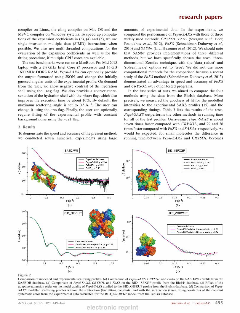
Figure 2Comparison of modelled and experimental scattering profiles. (a) Comparison of Pepsi-SAXS, CRYSOL and FoXS on the SASDAW3 profile from theSASBDB database. (b) Comparison of Pepsi-SAXS, CRYSOL and FoXS on the BID_1SPXGP profile from the BioIsis database. (c) Effect of theadaptive expansion order on the model quality of Pepsi-SAXS applied to the BID_GISRUP profile from the BioIsis database. (d) Comparison of Pepsi-SAXS modelled scattering profiles without the subtraction (two fitting constants) and with the subtraction (three fitting constants) of the constantsystematic error from the experimental data calculated for the BID_ZGDWKP model from the BioIsis database.

electronic reprint

larger, and the difference between Pepsi-SAXS and FoXSbecomes smaller. For large molecules, however, FoXS issignificantly slower compared with CRYSOL and Pepsi-SAXS. For example, Pepsi-SAXS computes the scatteringprofile for the BID_MnmGEP model about 62 times fastercompared with FoXS. We should mention that the reportedspeedup critically depends on the number of available CPUcores. Thus, we performed an additional artificial test andexecuted Pepsi-SAXS on a single CPU core. The averagerunning time over the BioIsis data set in this case was 0.36 s,which was still several times smaller compared with CRYSOLand other methods.

Regarding the accuracy of the modelled profiles, on averagePepsi-SAXS produces scattering curves that are very similar tothose computed by CRYSOL and FoXS, with approximatelythe same ! values, if these are computed for the same range ofscattering angles. We should specifically mention that in all ofthe tests we have restricted the maximum scattering anglesof Pepsi-SAXS to the default value of 0.5 A%1. This wasperformed for the rigorous comparison of the ! values withthe results of CRYSOL and FoXS. We should also mentionthat in some cases of noisy experimental data FoXS restrictsthe maximum scattering angles even further, thus producing !values that are higher on average. This, however, does not

necessarily mean that the quality of the computed profilesis worse compared with the results from Pepsi-SAXS andCRYSOL. SAStbx generally provides a significantly worsequality of fit and is thus excluded from the detailed compar-ison. Figs. 2(b), 2(c) and 2(d) show three examples of modelledscattering profiles from the BioIsis database. More plots,together with the residuals of the scattering profiles, can befound in Supplementary Fig. S1. Generally, we can concludethat Pepsi-SAXS computes scattering profiles that arecomparable to the other two methods. Below, we will alsostudy the effect of the adaptive resolution in comparison withCRYSOL in more detail.

We should also mention that a smaller ! value achievedusing a certain method for a scattering profile does notnecessarily mean a better quality of the computed profile.Generally, one should be concerned about possible flexibilityand conformational heterogeneity of the modelled proteins.Also, some of the models from the two benchmarks are notcrystallographic structures but were produced with molecular-dynamics simulations or MODELLER (Webb & Sali, 2014),for example. Therefore, small values of ! for some of themodels indicate potential overfitting of the experimentalprofiles rather than demonstrating the superiority of the fittingmethod. Finally, we should add that different methods use

research papers


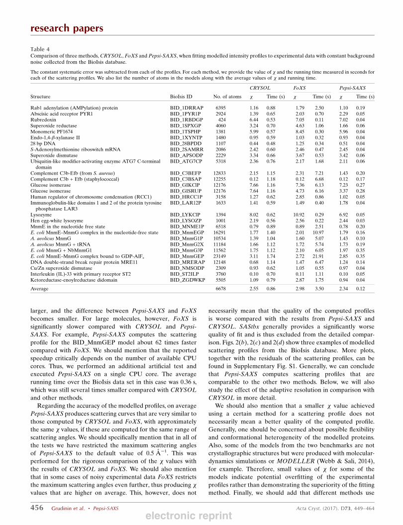
Table 4Comparison of three methods, CRYSOL, FoXS and Pepsi-SAXS, when fitting modelled intensity profiles to experimental data with constant backgroundnoise collected from the BioIsis database.

The constant systematic error was subtracted from each of the profiles. For each method, we provide the value of ! and the running time measured in seconds foreach of the scattering profiles. We also list the number of atoms in the models along with the average values of ! and running time.

CRYSOL FoXS Pepsi-SAXS

Structure BioIsis ID No. of atoms ! Time (s) ! Time (s) ! Time (s)

Rab1 adenylation (AMPylation) protein BID_1DRRAP 6395 1.16 0.88 1.79 2.50 1.10 0.19Abscisic acid receptor PYR1 BID_1PYR1P 2924 1.39 0.65 2.03 0.70 2.29 0.05Rubredoxin BID_1RBDGP 424 6.44 0.53 7.05 0.11 7.02 0.04Superoxide reductase BID_1SPXGP 4060 3.24 0.70 4.63 1.06 1.66 0.06Monomeric PF1674 BID_1TSPHP 1381 5.99 0.57 8.45 0.30 5.96 0.04Endo-1,4-)-xylanase II BID_1XYNTP 1480 0.95 0.59 1.03 0.32 0.93 0.0428 bp DNA BID_28BPDD 1107 0.44 0.48 1.25 0.34 0.51 0.04S-Adenosylmethionine riboswitch mRNA BID_2SAMRR 2086 2.42 0.60 2.46 0.47 2.45 0.04Superoxide dismutase BID_APSODP 2229 3.34 0.66 3.67 0.53 3.42 0.06Ubiquitin-like modifier-activating enzyme ATG7 C-terminal

domainBID_ATG7CP 5318 2.36 0.76 2.17 1.68 2.11 0.06

Complement C3b-Efb (from S. aureus) BID_C3BEFP 12833 2.15 1.15 2.31 7.21 1.43 0.20Complement C3b + Efb (staphylococcal) BID_C3BSAP 12255 0.12 1.18 0.12 6.68 0.12 0.17Glucose isomerase BID_GIKClP 12176 7.66 1.16 7.36 6.13 7.23 0.27Glucose isomerase BID_GISRUP 12176 7.64 1.16 4.73 6.16 3.37 0.28Human regulator of chromosome condensation (RCC1) BID_HRCC1P 3158 1.27 0.62 2.85 0.86 1.02 0.05Immunoglobulin-like domains 1 and 2 of the protein tyrosine

phosphatase LAR3BID_LAR12P 1633 1.41 0.59 1.49 0.40 1.78 0.04

Lysozyme BID_LYKClP 1394 8.02 0.62 10.92 0.29 6.92 0.05Hen egg-white lysozyme BID_LYSOZP 1001 2.19 0.56 2.56 0.22 2.44 0.03MnmE in the nucleotide free state BID_MNME1P 6518 0.79 0.89 0.89 2.51 0.78 0.20E. coli MnmE–MnmG complex in the nucleotide-free state BID_MnmEGP 16291 1.77 1.40 2.01 10.97 1.79 0.16A. aeolicus MnmG BID_MnmG1P 10534 1.39 1.04 1.60 5.07 1.43 0.10A. aeolicus MnmG + tRNA BID_MnmG2X 11184 1.66 1.12 1.72 5.74 1.73 0.19E. coli MnmG + NbMnmG1 BID_MnmG3P 11562 1.75 1.12 2.10 6.05 1.97 0.35E. coli MnmE–MnmG complex bound to GDP-AlFx BID_MnmGEP 23149 3.11 1.74 2.72 21.91 2.85 0.35DNA double-strand break repair protein MRE11 BID_MRERAP 12148 0.68 1.14 1.47 6.47 1.24 0.14Cu/Zn superoxide dismutase BID_NMSODP 2309 0.93 0.62 1.05 0.55 0.97 0.04Interleukin (IL)-33 with primary receptor ST2 BID_ST2ILP 3760 0.10 0.70 0.11 1.11 0.10 0.05Ketoreductase-enoylreductase didomain BID_ZGDWKP 5505 1.09 0.79 2.87 1.75 0.94 0.04

Average 6678 2.55 0.86 2.98 3.50 2.34 0.12

electronic reprint

different ranges of fitting parameters, and also differentmodels for the hydration shell, which consequently contributedifferently to the potential overfitting of experimental data.

Ideally, a reference data set of native structures supple-mented with experimental SAXS profiles along with non-native decoys should be established for the evaluation ofSAXS algorithms. Different methods can then be tested onthis data set by scoring the non-native decoys. The absence ofoverfitting in a SAXS method can be confirmed, for example,if the native structures have the lowest ! values among all ofthe scored decoys. To support our method, we should say thatwe use a small range of adjustable parameters compared withother methods such as CRYSOL and FoXS. Thus, we believethat Pepsi-SAXS does not have any significant overfitting ofexperimental data.

In the second series of tests, we compared the threemethods, excluding SAStbx, on the same data from BioIsis, butthis time measuring the goodness of fit for the modelledintensities to the experimental SAXS profiles and the corre-sponding timings for data with a constant systematic error (seeequation 3 in the Supporting Information). Table 4 lists thedetailed results of the tests. For all three of the methods, therunning time became only marginally larger. Regarding theaccuracy of the models, both Pepsi-SAXS and CRYSOLimproved the value of ! by about 9% on average, while FoXSunexpectedly worsened the averaged value of !. Fig. 2(d)shows an example of fitting for two profiles calculated byPepsi-SAXS with and without the constant systematic error inthe experimental curve. We can see a drastic improvement in

the model when subtracting the constant noise from theexperimental data.

In the third series of tests, we compared the four methodson the data from SASBDB. Here, we again first measured thegoodness of fit for the modelled intensities to the experimentalSAXS profiles (15) and the corresponding timings. Table 5 liststhe detailed results of the tests. Similarly to the previous tests,Pepsi-SAXS significantly outperforms the other methods inrunning time. Here, on average, Pepsi-SAXS is about fivetimes faster compared with CRYSOL, and 21 and 25 timesfaster compared with FoXS and SAStbx, respectively. Thespeedup in the running time of Pepsi-SAXS compared withthe other methods is somewhat smaller compared with theprevious tests owing to the on average higher expansionorders used here. More precisely, for SASBDB Pepsi-SAXSuses an average expansion order of 19, while for BioIsis it usesan order of 14. Regarding the accuracy of the modelledprofiles, on average Pepsi-SAXS, CRYSOL and FoXS achievethe same values of ! if these are computed using the samerange of scattering angles. SAStbx was not able to processhalf of the scattering profiles. It was again the slowest methodamong the four. Fig. 2(a) shows an example of modelledscattering profiles from this database. The model (SASDAW3)has a complex shape, thus we expected the quality of theCRYSOL modelled profile to be lower compared with profilesbuilt with FoXS and Pepsi-SAXS. Supplementary Fig. S1shows all of the scattering plots for SASBDB for the threemethods together with the residuals of the scatteringprofiles.

research papers


Table 5Comparison of four methods, CRYSOL, FoXS, SAStbx (using the three-dimensional Zernike technique and data-reduction option) and Pepsi-SAXS,when fitting modelled intensity profiles to experimental data collected from the SASBDB database.

For each method, we provide the value of ! and the running time measured in seconds for each of the scattering profiles. We also list the number of atoms in themodels along with the average values of ! and running time. SAStbx failed for some of the profiles; the corresponding values for ! and time are marked with a dash.

CRYSOL FoXS SAStbx Pepsi-SAXS

Structure SASBDB ID No. of atoms ! Time (s) ! Time (s) ! Time (s) ! Time (s)

Lysozyme C SASDAC2 1001 1.21 0.53 1.22 0.23 1.01 1.33 1.24 0.07Ubiquitin-60S ribosomal protein L40 SASDAQ2 602 3.08 0.51 3.10 0.16 3.67 1.14 3.00 0.07Myoglobin in PBS SASDAH2 1247 2.20 0.55 2.36 0.29 2.13 1.36 2.13 0.07Catalase in PBS SASDA92 16432 3.15 1.35 3.62 10.62 3.36 6.99 3.16 0.37Methyltransferase WbdD SASDAJ6 12662 1.22 1.11 1.04 6.94 — — 1.35 0.12Alcohol dehydrogenase in PBS SASDA52 10327 3.24 1.02 4.04 4.71 — — 2.94 0.26Calmodulin–peptide complex SASDAN4 1297 2.91 0.55 3.96 0.33 — — 3.48 0.08Psi-producing oxygenase A SASDA45 25761 9.70 1.89 13.83 24.30 — — 9.44 0.79Cysteine desulfurase IscS dimer SASDAV6 6118 1.30 0.80 1.88 2.14 — — 1.27 0.14Factor H CCP modules 12 to 13 SASDA25 951 1.70 0.52 1.73 0.28 1.27 1.90 1.56 0.07Heterotetramer of histidine protein kinase and response

regulatorSASDAA7 8124 1.05 0.87 1.06 3.47 1.77 5.80 1.05 0.11

ComE–comcde complex SASDAB7 5909 1.30 0.75 1.25 2.07 3.01 3.88 1.21 0.09LytTR–comcde complex SASDAC7 3605 1.18 0.63 1.17 1.15 — — 1.26 0.06Myomesin-1 SASDAK5 3231 1.59 0.64 1.65 1.15 2.23 3.52 1.82 0.09IcsS, IscU and CyaY dimeric complex SASDA27 9872 2.87 0.98 4.10 4.62 1.90 7.39 2.81 0.30Iron–sulfur cluster assembly scaffold IscU monomer SASDAW6 1014 1.19 0.53 1.24 0.26 — — 1.25 0.07Geminin–Cdt1 2:1 heterotrimer SASDAV3 2435 1.98 0.61 2.55 0.67 — — 2.61 0.10Geminin–Cdt1 4:2 heterohexamer SASDAW3 5362 3.35 0.78 3.16 1.99 3.29 5.03 2.94 0.17Apo XMRV RT SASDAV5 5366 1.12 0.77 1.19 1.89 0.87 5.40 1.13 0.18XMRV RT + DNA/RNA hybrid SASDAW5 6340 0.92 0.82 0.87 2.40 — — 0.91 0.20Protein CyaY monomer SASDAX6 863 1.15 0.53 1.21 0.20 — — 1.22 0.08Annexin-A4 SASDAJ5 2510 5.16 0.61 5.26 0.65 3.93 2.06 5.09 0.08Pyruvate decarboxylase SASDAX2 17157 0.81 1.36 0.82 11.24 0.90 8.35 0.83 0.29

Average 6443 2.32 0.81 2.71 3.56 2.26 4.17 2.33 0.17

electronic reprint

In the fourth series of tests, we again compared the threemethods, excluding SAStbx, on the data from SASBDB andmeasured the goodness of fit with a constant systematic error(see equation 3 in the Supporting Information) and thecorresponding timings. Table 6 lists the detailed results of thetests. As before, the running time becomes only marginallylarger. Regarding the accuracy of the models, Pepsi-SAXSimproves the value of ! by 8% on average, CRYSOL improvesit by 6% and FoXS again shows no improvement in fit.

For the fifth test, we decided to compare the running time ofthe four methods if a user computes a scattering profilewithout fitting it to the experimental data. Here, we consid-ered two scenarios: a profile with 51 points, as used to be thedefault option in CRYSOL, and a profile with 512 points,which better corresponds to modern experimental measure-ments. Table 7 lists the timings for all four methods run onatomic models from the BioIsis and SASBDB databases. Forthe 51-point profile, Pepsi-SAXS is on average about threetimes faster compared with CRYSOL, and 19 and 27 timesfaster compared with FoXS and SAStbx, respectively. With the512-point profile, Pepsi-SAXS, FoXs and SAStbx increase thetimings only marginally. However, the running time ofCRYSOL depends linearly on the number of points in thescattering profile. Therefore, its timing increases about tentimes.

In the sixth series of tests, we compared the effect of theadaptive choice of the multipole expansion order using datafrom the BioIsis and SASBDB databases. To do so, we firstfixed the expansion order to the value of 15, which is used by

default in CRYSOL, and ran Pepsi-SAXS in comparison withCRYSOL. We then chose the value of the expansion orderadaptively according to (14) and ran the two programs again.Table 8 lists the details of the comparisons. As we can see fromthis table, using the default expansion order of 15, Pepsi-SAXSdemonstrates a very similar quality of models compared withCRYSOL, with a slightly smaller value of !. Adaptive reso-lution lowers the value of ! for the two methods: by about 1%for CRYSOL and about 2% for Pepsi-SAXS. We attribute themore pronounced effect of the adaptive resolution in Pepsi-SAXS to the different model of the hydration shell in ourmethod. Fig. 2(c) shows an example of scattering profilesplotted at a different expansion order in comparison with theexperimental curve for a large molecule (BID_GISRUP). Wecan see a pronounced difference between the curves at largevalues of q, which corresponds to a fine resolution in real spacethat is not well encoded using low-multipole expansion orders.All scattering profiles for experimental data collected from theBioIsis and SASBDB databases and computed using Pepsi-SAXS, CRYSOL and FoXS can be found in SupplementaryFig. S1.

Finally, in the seventh series of tests, we compared thevalues of two adjustable parameters, r0 and #", for the threemethods, excluding SAStbx, on data from the BioIsis andSASBDB databases. In the case of FoXS, we computed thevalues of r0 and #" by rescaling its internal fitting parametersc1 and c2 as suggested by the authors (Schneidman-Duhovny etal., 2010). Table 9 lists the adjustable parameters along withthe mean values and the standard deviations for the three

research papers


Table 6Comparison of three methods, CRYSOL, FoXS and Pepsi-SAXS, when fitting modelled intensity profiles to experimental data with constant backgroundnoise collected from the SASBDB database.

The constant systematic error was subtracted from each of the profiles. For each method, we provide the value of ! and the running time measured in seconds foreach of the scattering profiles. We also list the number of atoms in the models along with the average values of ! and running time.


Structure SASBDB ID No. of atoms ! Time (s) ! Time (s) ! Time (s)

Lysozyme C SASDAC2 1001 1.21 0.61 1.22 0.24 1.23 0.09Ubiquitin-60S ribosomal protein L40 SASDAQ2 602 3.07 0.58 3.10 0.16 2.99 0.09Myoglobin in PBS SASDAH2 1247 2.10 0.63 2.40 0.29 2.10 0.09Catalase in PBS SASDA92 16432 2.93 1.44 4.07 10.53 2.97 0.39Methyltransferase WbdD SASDAJ6 12662 1.14 1.17 1.13 6.98 1.19 0.13Alcohol dehydrogenase in PBS SASDA52 10327 2.54 1.11 5.41 4.72 2.46 0.28Calmodulin–peptide complex SASDAN4 1297 2.32 0.61 4.05 0.33 3.12 0.11Psi-producing oxygenase A SASDA45 25761 9.67 1.98 14.95 24.33 8.48 0.82Cysteine desulfurase IscS dimer SASDAV6 6118 1.28 0.85 1.93 2.13 1.27 0.15Factor H CCP modules 12 to 13 SASDA25 951 1.42 0.59 1.74 0.27 1.25 0.09Heterotetramer of histidine protein kinase and response

regulatorSASDAA7 8124 1.04 0.93 1.07 3.47 1.05 0.14

ComE–comcde complex SASDAB7 5909 1.18 0.82 1.32 2.04 1.11 0.09LytTR–comcde complex SASDAC7 3605 1.16 0.69 1.17 1.15 1.26 0.07Myomesin-1 SASDAK5 3231 1.57 0.72 1.66 1.16 1.64 0.10IcsS, IscU and CyaY dimeric complex SASDA27 9872 2.62 1.06 5.17 4.63 2.57 0.33Iron–sulfur cluster assembly scaffold IscU monomer SASDAW6 1014 1.19 0.61 1.26 0.26 1.25 0.09Geminin–Cdt1 2:1 heterotrimer SASDAV3 2435 1.94 0.62 3.13 0.65 1.80 0.12Geminin–Cdt1 4:2 heterohexamer SASDAW3 5362 2.94 0.88 3.19 2.04 2.90 0.19Apo XMRV RT SASDAV5 5366 1.11 0.85 1.21 1.94 1.10 0.21XMRV RT + DNA/RNA hybrid SASDAW5 6340 0.90 0.91 0.87 2.35 0.90 0.23Protein CyaY monomer SASDAX6 863 1.10 0.60 1.21 0.20 1.12 0.09Annexin-A4 SASDAJ5 2510 5.09 0.67 5.28 0.63 5.06 0.11Pyruvate decarboxylase SASDAX2 17157 0.81 1.43 0.83 11.26 0.82 0.30

electronic reprint

methods. We can see that all of the methods agree on anaverage value of the effective atomic radius r0 of 1.64 A.However, the standard deviation of this parameter in FoXSand Pepsi-SAXS is only 0.05 A, which constitutes 3% of theaverage value and is several times smaller compared with thestandard deviation of 0.18 A in CRYSOL. We should note that

if we double the width of the search window for the r0 para-meter to make it more comparable with the CRYSOL settings,the quality of fit to the experimental data improves onlymarginally (see Supplementary Table S2).

Regarding the second adjustable parameter, the contrast ofthe hydration shell #", all of the methods provide different

research papers


Table 7Comparison of four methods, CRYSOL, FoXS, SAStbx (using the three-dimensional Zernike technique) and Pepsi-SAXS, when calculating intensityprofiles for models collected from the BioIsis and SASBDB databases.

No fitting to experimental data was performed. For each method, we provide two running times measured in seconds when calculating the intensity profile with 512points and with 51 points, correspondingly. We also list the number of atoms in the models along with the average values of running times. SAStbx failed for someof the profiles; the corresponding values of timings are marked with dashes.

Structure Database ID No. of atoms CRYSOL FoXS SAXStbx Pepsi-SAXS

Rab1 adenylation (AMPylation) protein BID_1DRRAP 6395 3.55/0.44 2.46/2.05 5.24/5.11 0.14/0.13Abscisic acid receptor PYR1 BID_1PYR1P 2924 1.80/0.25 0.69/0.62 2.18/2.14 0.04/0.04Rubredoxin BID_1RBDGP 424 0.70/0.13 0.10/0.08 0.99/0.96 0.01/0.01Superoxide reductase BID_1SPXGP 4060 2.25/0.31 1.04/0.97 2.33/2.26 0.05/0.05Monomeric PF1674 BID_1TSPHP 1381 1.14/0.17 0.28/0.24 1.90/1.87 0.02/0.02Endo-1,4-)-xylanase II BID_1XYNTP 1480 1.16/0.18 0.31/0.26 1.39/1.38 0.02/0.0228 bp DNA BID_28BPDD 1107 0.97/0.16 0.35/0.19 1.71/1.69 0.02/0.03S-Adenosylmethionine riboswitch mRNA BID_2SAMRR 2086 1.43/0.21 0.46/0.37 1.85/1.83 0.03/0.04Superoxide dismutase BID_APSODP 2229 1.50/0.22 0.52/0.43 1.83/1.83 0.03/0.04Ubiquitin-like modifier-activating enzyme ATG7 C-terminal

domainBID_ATG7CP 5318 2.86/0.38 1.71/1.50 3.90/3.97 0.09/0.09

Complement C3b-Efb (from S. aureus) BID_C3BEFP 12833 6.65/0.81 7.20/6.79 10.16/10.19 0.35/0.36Complement C3b + Efb (staphylococcal) BID_C3BSAP 12255 6.47/0.77 6.59/6.13 8.23/8.05 0.32/0.33Glucose isomerase BID_GIKClP 12176 5.87/0.73 6.08/5.88 5.47/5.52 0.25/0.24Glucose isomerase BID_GISRUP 12176 6.09/0.73 6.12/5.90 6.01/6.10 0.25/0.24Human regulator of chromosome condensation (RCC1) BID_HRCC1P 3158 1.91/0.26 0.84/0.71 2.81/2.79 0.05/0.04Immunoglobulin-like domains 1 and 2 of the protein tyrosine

phosphatase LAR3BID_LAR12P 1633 1.25/0.19 0.41/0.30 1.98/1.98 0.03/0.03

Lysozyme BID_LYKClP 1394 1.13/0.17 0.28/0.24 1.38/1.29 0.02/0.02Hen egg-white lysozyme BID_LYSOZP 1001 0.96/0.15 0.21/0.18 1.30/1.19 0.02/0.02MnmE in the nucleotide-free state BID_MNME1P 6518 3.46/0.44 2.42/2.10 4.43/4.48 0.13/0.13E. coli MnmE–MnmG complex in the nucleotide-free state BID_MnmEGP 16291 8.42/0.98 10.76/10.11 10.33/10.87 0.55/0.55A. aeolicus MnmG BID_MnmG1P 10534 5.56/0.68 5.12/4.72 9.35/9.46 0.33/0.28A. aeolicus MnmG + tRNA BID_MnmG2X 11184 5.67/0.68 5.66/5.16 7.50/7.36 0.32/0.28E. coli MnmG + NbMnmG1 BID_MnmG3P 11562 6.17/0.74 6.14/5.60 8.14/7.99 0.31/0.33E. coli MnmE–MnmG complex bound to GDP-AlFx BID_MnmGEP 23149 12.29/1.39 21.79/20.63 5.80/6.03 1.84/1.29DNA double-strand break repair protein MRE11 BID_MRERAP 12148 6.18/0.75 6.41/5.98 7.75/7.68 0.35/0.30Cu/Zn superoxide dismutase BID_NMSODP 2309 1.56/0.25 0.56/0.46 2.01/2.04 0.04/0.04Interleukin (IL)-33 with primary receptor ST2 BID_ST2ILP 3760 2.20/0.31 1.08/0.89 3.09/2.93 0.07/0.07Ketoreductase-enoylreductase didomain BID_ZGDWKP 5505 2.98/0.38 1.75/1.58 3.47/3.38 0.10/0.10Lysozyme C SASDAC2 1001 0.97/0.16 0.21/0.17 1.28/1.27 0.02/0.02Ubiquitin-60S ribosomal protein L40 SASDAQ2 602 0.79/0.13 0.14/0.10 1.14/1.11 0.01/0.01Myoglobin in PBS SASDAH2 1247 1.08/0.17 0.26/0.21 1.37/1.34 0.02/0.02Catalase in PBS SASDA92 16432 8.02/0.96 10.64/10.22 7.33/6.94 0.34/0.32Methyltransferase WbdD SASDAJ6 12662 6.70/0.80 6.94/6.49 9.23/8.85 0.39/0.38Alcohol dehydrogenase in PBS SASDA52 10327 5.20/0.65 4.65/4.46 5.19/5.07 0.22/0.21Calmodulin–peptide complex SASDAN4 1297 1.14/0.18 0.31/0.22 —/— 0.02/0.03Psi-producing oxygenase A SASDA45 25761 13.11/1.50 24.28/23.6 13.95/14.2 0.87/0.84Cysteine desulfurase IscS dimer SASDAV6 6118 3.22/0.41 2.15/1.95 3.90/3.71 0.09/0.10Factor H CCP modules 12 to 13 SASDA25 951 0.94/0.15 0.25/0.16 1.90/1.90 0.02/0.02Heterotetramer of histidine protein kinase and response

regulatorSASDAA7 8124 4.24/0.53 3.49/3.03 6.00/5.72 0.19/0.18

ComE–comcde complex SASDAB7 5909 3.20/0.40 2.05/1.83 4.14/4.00 0.11/0.10LytTR–comcde complex SASDAC7 3605 2.16/0.28 1.13/0.86 —/— 0.07/0.07Myomesin-1 SASDAK5 3231 2.04/0.28 1.11/0.76 3.60/3.57 0.09/0.09IcsS, IscU and CyaY dimeric complex SASDA27 9872 4.99/0.61 4.59/4.19 7.24/7.49 0.25/0.23Iron–sulfur cluster assembly scaffold IscU monomer SASDAW6 1014 0.99/0.16 0.26/0.17 —/— 0.02/0.02Geminin–Cdt1 2:1 heterotrimer SASDAV3 2435 1.65/0.23 0.65/0.50 2.29/2.18 0.04/0.04Geminin–Cdt1 4:2 heterohexamer SASDAW3 5362 3.16/0.39 1.99/1.60 4.94/4.97 0.12/0.11Apo XMRV RT SASDAV5 5366 3.06/0.40 1.95/1.57 5.46/5.65 0.15/0.14XMRV RT + DNA/RNA hybrid SASDAW5 6340 3.45/0.46 2.37/2.02 5.34/5.25 0.16/0.15Protein CyaY monomer SASDAX6 863 0.95/0.15 0.19/0.14 —/— 0.02/0.02Annexin-A4 SASDAJ5 2510 1.65/0.23 0.62/0.51 2.04/1.98 0.03/0.03Pyruvate decarboxylase SASDAX2 17157 8.41/1.01 11.22/10.95 8.58/8.52 0.40/0.38

Average 6572.0 3.59/0.45 3.51/3.25 4.63/4.60 0.18/0.17

electronic reprint

mean values. More precisely, CRYSOL allows variationof #" between 0 and 60 e nm%3, with an average of22.4 + 21.7 e nm%3. FoXS allows negative values of #" in therange ,27 * #" * 54 e nm%3. Thus, its average #" is lower

compared with that computed by CRYSOL and equals 16.6 +22.2 e nm%3. In our model, by default, we allow only positivevalues of #" up to one tenth of the bulk density value of33.4 e nm%3. As a result, our mean value of the contrast of the

research papers


Table 8Comparison of CRYSOL with Pepsi-SAXS when using adaptive multipole expansion orders.

Experimental data were collected from the BioIsis and SASBDB databases. For each method, we provide the value of ! and the running time measured in secondswhen using the default expansion order of 15 and the adaptive expansion order. We also list the number of atoms in the models and the order of the adaptivemultipole expansion, along with the average values of ! and running time.

Expansion order = 15 Adaptive expansion order

CRYSOL Pepsi-SAXS CRYSOL Pepsi-SAXS

Structure Database IDNo. ofatoms !

Time(s) !

Time(s) Order !

Time(s) !

Time(s)

Rab1 adenylation (AMPylation) protein BID_1DRRAP 6395 1.98 0.82 1.55 0.13 24 1.79 1.10 1.51 0.18Abscisic acid receptor PYR1 BID_1PYR1P 2924 1.39 0.59 2.30 0.05 10 1.39 0.51 2.33 0.04Rubredoxin BID_1RBDGP 424 7.61 0.45 7.42 0.03 5 7.78 0.38 7.24 0.03Superoxide reductase BID_1SPXGP 4060 3.40 0.63 1.67 0.06 11 3.40 0.57 1.67 0.05Monomeric PF1674 BID_1TSPHP 1381 6.28 0.49 6.13 0.04 7 6.28 0.43 6.22 0.03Endo-1,4-)-xylanase II BID_1XYNTP 1480 0.99 0.50 0.93 0.04 7 0.99 0.43 0.93 0.0328 bp DNA BID_28BPDD 1107 0.49 0.48 0.57 0.04 11 0.49 0.46 0.56 0.03S-Adenosylmethionine riboswitch mRNA BID_2SAMRR 2086 2.42 0.53 2.51 0.05 9 2.40 0.46 2.46 0.03Superoxide dismutase BID_APSODP 2229 3.45 0.57 3.58 0.06 15 3.45 0.59 3.58 0.06Ubiquitin-like modifier-activating enzyme ATG7 C-terminal

domainBID_ATG7CP 5318 2.54 0.71 2.23 0.08 13 2.53 0.66 2.19 0.06

Complement C3b-Efb (from S. aureus) BID_C3BEFP 12833 2.41 1.15 1.57 0.16 18 2.45 1.34 1.63 0.19Complement C3b + Efb (staphylococcal) BID_C3BSAP 12255 0.12 1.10 0.12 0.14 18 0.12 1.28 0.12 0.17Glucose isomerase BID_GIKCLP 12176 7.83 1.09 6.85 0.15 23 7.86 1.47 7.34 0.26Glucose isomerase BID_GISRUP 12176 7.99 1.09 5.43 0.15 23 6.39 1.45 3.38 0.26Human regulator of chromosome condensation (RCC1) BID_HRCC1P 3158 1.29 0.59 1.63 0.06 11 1.29 0.53 1.59 0.05Immunoglobulin-like domains 1 and 2 of the protein tyrosine

phosphatase LAR3BID_LAR12P 1633 1.44 0.51 1.90 0.05 10 1.43 0.48 1.85 0.03

Lysozyme BID_LYKCLP 1394 9.39 0.53 9.42 0.05 11 9.39 0.50 9.41 0.04Hen egg-white lysozyme BID_LYSOZP 1001 2.54 0.49 2.60 0.04 8 2.54 0.43 2.62 0.03MnmE in the nucleotide-free state BID_MNME1P 6518 0.89 0.82 0.84 0.14 24 0.86 1.13 0.85 0.18E. coli MnmE–MnmG complex in the nucleotide-free state BID_MnmEGP 16291 1.86 1.31 1.85 0.18 16 1.85 1.38 1.84 0.15A. aeolicus MnmG BID_MnmG1P 10534 1.40 1.04 1.45 0.13 11 1.39 0.85 1.44 0.10A. aeolicus MnmG + tRNA BID_MnmG2X 11184 1.70 1.04 1.76 0.15 21 1.71 1.33 1.75 0.18E. coli MnmG + NbMnmG1 BID_MnmG3P 11562 1.79 1.07 3.13 0.14 27 1.78 1.69 2.05 0.35E. coli MnmE–MnmG complex bound to GDP-AlFx BID_MnmGEP 23149 3.16 1.71 2.82 0.26 19 3.20 2.19 2.87 0.35DNA double-strand break repair protein MRE11 BID_MRERAP 12148 0.72 1.08 1.32 0.14 17 0.72 1.18 1.29 0.14Cu/Zn superoxide dismutase BID_NMSODP 2309 1.04 0.55 0.96 0.05 10 1.05 0.49 0.97 0.04Interleukin (IL)-33 with primary receptor ST2 BID_ST2ILP 3760 0.10 0.64 0.11 0.07 13 0.10 0.59 0.11 0.05Ketoreductase-enoylreductase didomain BID_ZGDWKP 5505 2.00 0.72 1.62 0.07 12 2.01 0.64 1.61 0.04Lysozyme C SASDAC2 1001 1.21 0.53 1.24 0.08 11 1.21 0.50 1.24 0.07Ubiquitin-60S ribosomal protein L40 SASDAQ2 602 3.08 0.51 2.99 0.08 10 3.08 0.47 3.00 0.07Myoglobin in PBS SASDAH2 1247 2.20 0.55 2.12 0.08 12 2.20 0.52 2.13 0.07Catalase in PBS SASDA92 16432 3.15 1.34 3.40 0.22 25 3.10 2.02 3.16 0.37Methyltransferase WbdD SASDAJ6 12662 1.22 1.11 1.23 0.17 13 1.30 1.00 1.35 0.12Alcohol dehydrogenase in PBS SASDA52 10327 3.24 1.03 2.95 0.17 23 3.16 1.36 2.94 0.26Calmodulin–peptide complex SASDAN4 1297 2.91 0.55 3.48 0.09 14 2.92 0.54 3.48 0.09Psi-producing oxygenase A SASDA45 25761 9.70 1.88 8.78 0.33 29 9.79 3.63 9.44 0.79Cysteine desulfurase IscS dimer SASDAV6 6118 1.30 0.80 1.28 0.13 20 1.30 0.91 1.27 0.14Factor H CCP modules 12 to 13 SASDA25 951 1.70 0.51 1.56 0.08 13 1.70 0.50 1.56 0.07Heterotetramer of histidine protein kinase and response

regulatorSASDAA7 8124 1.05 0.87 1.10 0.11 20 1.01 1.06 1.05 0.12

ComE–comcde complex SASDAB7 5909 1.30 0.75 1.23 0.09 17 1.27 0.80 1.21 0.09LytTR–comcde complex SASDAC7 3605 1.18 0.64 1.29 0.07 16 1.15 0.66 1.26 0.06Myomesin-1 SASDAK5 3231 1.59 0.63 1.76 0.08 21 1.65 0.73 1.82 0.09IcsS, IscU and CyaY dimeric complex SASDA27 9872 2.87 0.99 2.77 0.17 26 2.85 1.42 2.81 0.30Iron–sulfur cluster assembly scaffold IscU monomer SASDAW6 1014 1.19 0.56 1.25 0.09 13 1.19 0.52 1.25 0.07Geminin–Cdt1 2:1 heterotrimer SASDAV3 2435 1.98 0.62 2.57 0.10 17 1.99 0.64 2.61 0.10Geminin–Cdt1 4:2 heterohexamer SASDAW3 5362 3.35 0.77 2.85 0.13 24 3.17 1.10 2.94 0.17Apo XMRV RT SASDAV5 5366 1.12 0.78 1.16 0.13 23 1.10 1.00 1.13 0.18XMRV RT + DNA/RNA hybrid SASDAW5 6340 0.92 0.82 0.91 0.14 23 0.92 1.06 0.91 0.20Protein CyaY monomer SASDAX6 863 1.15 0.54 1.22 0.08 11 1.15 0.50 1.22 0.08Annexin-A4 SASDAJ5 2510 5.16 0.60 5.08 0.10 16 5.16 0.63 5.09 0.09Pyruvate decarboxylase SASDAX2 17157 0.82 1.36 0.82 0.18 24 0.82 2.01 0.83 0.29

Average 6572.0 2.58 0.81 2.50 0.11 16.18 2.55 0.94 2.45 0.14

electronic reprint

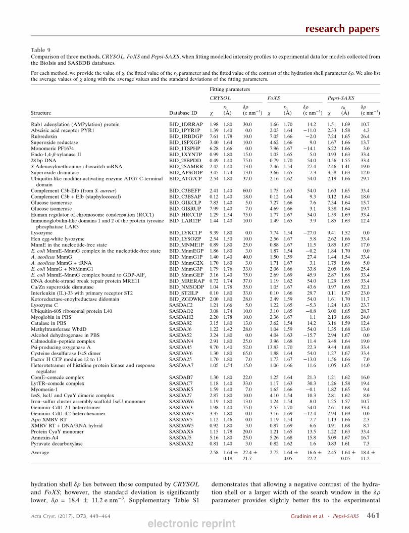
hydration shell #" lies between those computed by CRYSOLand FoXS; however, the standard deviation is significantlylower, #" = 18.4 + 11.2 e nm%3. Supplementary Table S1

demonstrates that allowing a negative contrast of the hydra-tion shell or a larger width of the search window in the #"parameter provides slightly better fits to the experimental

research papers


Table 9Comparison of three methods, CRYSOL, FoXS and Pepsi-SAXS, when fitting modelled intensity profiles to experimental data for models collected fromthe BioIsis and SASBDB databases.

For each method, we provide the value of !, the fitted value of the r0 parameter and the fitted value of the contrast of the hydration shell parameter #". We also listthe average values of ! along with the average values and the standard deviations of the fitting parameters.

Fitting parameters


Structure Database ID !r0

(A)#"(e nm%1) !

r0

(A)#"(e nm%1) !

r0

(A)#"(e nm%1)

Rab1 adenylation (AMPylation) protein BID_1DRRAP 1.98 1.80 30.0 1.66 1.70 14.2 1.51 1.69 10.7Abscisic acid receptor PYR1 BID_1PYR1P 1.39 1.40 0.0 2.03 1.64 %11.0 2.33 1.58 4.3Rubredoxin BID_1RBDGP 7.61 1.78 10.0 7.05 1.66 %2.0 7.24 1.65 26.4Superoxide reductase BID_1SPXGP 3.40 1.64 10.0 4.62 1.66 9.0 1.67 1.66 13.7Monomeric PF1674 BID_1TSPHP 6.28 1.66 0.0 7.96 1.67 %14.1 6.22 1.66 3.0Endo-1,4-)-xylanase II BID_1XYNTP 0.99 1.80 15.0 1.03 1.65 5.0 0.93 1.63 33.428 bp DNA BID_28BPDD 0.49 1.40 75.0 0.79 1.70 54.0 0.56 1.55 33.4S-Adenosylmethionine riboswitch mRNA BID_2SAMRR 2.42 1.40 13.0 2.46 1.54 27.4 2.46 1.41 19.0Superoxide dismutase BID_APSODP 3.45 1.74 13.0 3.66 1.65 7.3 3.58 1.63 12.0Ubiquitin-like modifier-activating enzyme ATG7 C-terminal

domainBID_ATG7CP 2.54 1.80 37.0 2.16 1.62 54.0 2.19 1.66 29.7

Complement C3b-Efb (from S. aureus) BID_C3BEFP 2.41 1.40 60.0 1.75 1.63 54.0 1.63 1.65 33.4Complement C3b + Efb (staphylococcal) BID_C3BSAP 0.12 1.40 18.0 0.12 1.64 9.3 0.12 1.64 18.0Glucose isomerase BID_GIKCLP 7.83 1.40 5.0 7.27 1.66 7.6 7.34 1.64 15.7Glucose isomerase BID_GISRUP 7.99 1.40 7.0 4.69 1.66 3.1 3.38 1.64 19.7Human regulator of chromosome condensation (RCC1) BID_HRCC1P 1.29 1.54 75.0 1.77 1.67 54.0 1.59 1.69 33.4Immunoglobulin-like domains 1 and 2 of the protein tyrosine

phosphatase LAR3BID_LAR12P 1.44 1.40 10.0 1.49 1.65 3.9 1.85 1.63 12.4

Lysozyme BID_LYKCLP 9.39 1.80 0.0 7.74 1.54 %27.0 9.41 1.52 0.0Hen egg-white lysozyme BID_LYSOZP 2.54 1.50 10.0 2.56 1.67 5.8 2.62 1.66 33.4MnmE in the nucleotide-free state BID_MNME1P 0.89 1.80 25.0 0.88 1.67 11.5 0.85 1.67 17.0E. coli MnmE–MnmG complex in the nucleotide-free state BID_MnmEGP 1.86 1.80 3.0 1.87 1.54 %0.2 1.84 1.70 0.0A. aeolicus MnmG BID_MnmG1P 1.40 1.40 40.0 1.50 1.59 27.4 1.44 1.54 33.4A. aeolicus MnmG + tRNA BID_MnmG2X 1.70 1.80 3.0 1.71 1.67 3.1 1.75 1.66 5.0E. coli MnmG + NbMnmG1 BID_MnmG3P 1.79 1.76 33.0 2.06 1.66 33.8 2.05 1.66 25.4E. coli MnmE–MnmG complex bound to GDP-AlFx BID_MnmGEP 3.16 1.40 75.0 2.69 1.69 45.9 2.87 1.68 33.4DNA double-strand break repair protein MRE11 BID_MRERAP 0.72 1.74 37.0 1.19 1.62 54.0 1.29 1.65 33.4Cu/Zn superoxide dismutase BID_NMSODP 1.04 1.78 35.0 1.05 1.67 43.6 0.97 1.66 32.1Interleukin (IL)-33 with primary receptor ST2 BID_ST2ILP 0.10 1.80 33.0 0.10 1.66 29.7 0.11 1.67 23.0Ketoreductase-enoylreductase didomain BID_ZGDWKP 2.00 1.80 28.0 2.49 1.59 54.0 1.61 1.70 11.7Lysozyme C SASDAC2 1.21 1.66 5.0 1.22 1.65 %5.3 1.24 1.63 23.7Ubiquitin-60S ribosomal protein L40 SASDAQ2 3.08 1.74 10.0 3.10 1.65 %0.8 3.00 1.65 28.7Myoglobin in PBS SASDAH2 2.20 1.78 10.0 2.36 1.67 1.1 2.13 1.66 24.0Catalase in PBS SASDA92 3.15 1.80 13.0 3.62 1.54 14.2 3.16 1.59 12.4Methyltransferase WbdD SASDAJ6 1.22 1.42 28.0 1.04 1.59 54.0 1.35 1.68 13.0Alcohol dehydrogenase in PBS SASDA52 3.24 1.80 0.0 4.04 1.63 %15.7 2.94 1.67 0.0Calmodulin–peptide complex SASDAN4 2.91 1.80 25.0 3.96 1.68 11.4 3.48 1.64 19.0Psi-producing oxygenase A SASDA45 9.70 1.40 52.0 13.83 1.70 22.3 9.44 1.68 33.4Cysteine desulfurase IscS dimer SASDAV6 1.30 1.80 65.0 1.88 1.64 54.0 1.27 1.67 33.4Factor H CCP modules 12 to 13 SASDA25 1.70 1.80 7.0 1.73 1.67 %13.0 1.56 1.66 7.0Heterotetramer of histidine protein kinase and response

regulatorSASDAA7 1.05 1.54 15.0 1.06 1.66 11.6 1.05 1.65 14.0

ComE–comcde complex SASDAB7 1.30 1.80 22.0 1.25 1.64 21.3 1.21 1.62 16.0LytTR–comcde complex SASDAC7 1.18 1.40 33.0 1.17 1.63 30.3 1.26 1.58 19.4Myomesin-1 SASDAK5 1.59 1.40 7.0 1.65 1.66 %0.1 1.82 1.65 9.4IcsS, IscU and CyaY dimeric complex SASDA27 2.87 1.80 10.0 4.10 1.54 10.3 2.81 1.62 8.0Iron–sulfur cluster assembly scaffold IscU monomer SASDAW6 1.19 1.80 13.0 1.24 1.54 8.0 1.25 1.57 10.7Geminin–Cdt1 2:1 heterotrimer SASDAV3 1.98 1.40 75.0 2.55 1.70 54.0 2.61 1.68 33.4Geminin–Cdt1 4:2 heterohexamer SASDAW3 3.35 1.80 0.0 3.16 1.69 %12.4 2.94 1.69 0.0Apo XMRV RT SASDAV5 1.12 1.46 0.0 1.19 1.54 7.7 1.13 1.66 2.3XMRV RT + DNA/RNA hybrid SASDAW5 0.92 1.80 3.0 0.87 1.69 6.6 0.91 1.68 8.7Protein CyaY monomer SASDAX6 1.15 1.78 20.0 1.21 1.65 13.5 1.22 1.63 33.4Annexin-A4 SASDAJ5 5.16 1.80 25.0 5.26 1.68 15.8 5.09 1.67 16.7Pyruvate decarboxylase SASDAX2 0.81 1.40 3.0 0.82 1.62 1.6 0.83 1.61 7.3

Average 2.58 1.64 +0.18

22.4 +21.7

2.72 1.64 +0.05

16.6 +22.2

2.45 1.64 +0.05

18.4 +11.2

electronic reprint

profiles. However, this choice of adjustable parameters mightoverfit the actual experimental data.

4. Discussion

In this section, we will first discuss the general considerationsthat affect the performance of our method, and we will thenalso examine the particular details of the implementation.Given the number of atoms in a model N, and the number ofpoints in the scattering profile M, our Pepsi-SAXS approachachieves the asymptotically best performance, in terms of Nand M, of O(N + M). Methods with such a performance aregenerally considered as a class of linear scaling methods.However, when speaking about asymptotic complexity, weshould also take into account the effect of the expansionorder L, such that the complexity of our method becomesO(L3N + M). In principle, according to (14), the optimalexpansion order L is proportional to the linear size of themolecular model, and thus L3 is proportional to the number ofatoms in the model N. Therefore, effectively, the asymptoticcomplexity of the Pepsi-SAXS method, as well as the three-dimensional Zernike and some other multipole expansion-based approaches, reads O(N 2 + M), with the same leadingterm O(N 2) as in the complexity of the binning techniques forthe Debye equation, for example that implemented in FoXS.We should also note that the complexity of the recent versionof CRYSOL for typical values of L and M is higher comparedwith the complexity of Pepsi-SAXS and the three-dimensionalZernike approach, since CRYSOL computes scatteringamplitudes at a fixed number of scattering points. Regardlessof the O(N 2) asymptotic complexity of our method, it has avery low prefactor compared with Debye-based techniques,and thus it is much faster in practice. Also, Pepsi-SAXS andother multipole expansion-based approaches do not requirethe single-Gaussian approximation of the form factors, whichincreases the accuracy of these methods.

One of the factors that strongly affects the quality of thescattering model is the description of the hydration shell. Ourmethod (see Fig. 1) uses a grid-based approximation, with theeffective width varying from 3 to 5 A depending on the size ofthe modelled molecule. The maximum allowed width of 5 A issomewhat larger compared with the value used in CRYSOLand some other methods. However, we use a smaller searchwindow for the value of the relative contrast of the hydrationshell compared with CRYSOL and FoXS, for example. Also,this value agrees with more recent developments, for example,with the hydration-shell intensities computed from MDtrajectories (Park et al., 2009), where a width of 7 A or larger issuggested. Finally, a recent X-ray reflectivity study suggests ahydration-gap width of up to 9 A (Chattopadhyay et al., 2010).Our representation of the hydration shell describes internalwater cavities and surface pockets more accurately comparedwith the models built using a two-dimensional angularenvelope function, for example that in CRYSOL. Figs. 2(a)and 2(b) demonstrate the overall superior quality of modelledscattering profiles built with Pepsi-SAXS for models withcomplex shapes. On the other hand, our hydration model is

more prone to overfitting. We should mention that theshortcomings of the simplified two-dimensional angularrepresentation of the hydration layer were discussed in theoriginal CRYSOL paper (Svergun et al., 1995), where it wasclaimed that it still correctly describes the outer hydrationshell.

Another factor that influences the quality of the scatteringmodel is the description of the excluded solvent. Our modelof the excluded solvent is derived from the approximationintroduced by Fraser et al. (1978) and closely follows themodel used in CRYSOL. More precisely, we use the first-orderMaclaurin expansion in the scaling parameter (12) of themodel of Fraser and coworkers. We have also run tests usinga more detailed second-order expansion approximation;however, it did not provide any notable improvement in themodel quality. The zero-order q-independent approximation,surprisingly, does not change the goodness of fit either. Weattribute these marginal differences between the models of theexcluded solvent to a relatively high level of noise of thecurrent profiles at large scattering angles.

The goodness of fit between the modelled intensities andthe experimental profiles is influenced by the number of fittingparameters in the modelled scattering profile. The Aqua-SAXS, FoXS and SAStbx methods effectively use the sameadjustable parameters as Pepsi-SAXS and CRYSOL. Themethod of Zheng & Tekpinar (2011) uses a single adjustableparameter: the relative contrast of the hydration shell. TheAXES procedure replaces the atomic radii multiplier and thetotal excluded volume, which are applied to the model data,by the solvent/buffer rescaling factor and the constant offsetapplied to the measured data. Thanks to the partial scatteringintensities (see equations 1 and 2 in the Supporting Informa-tion), the computation of the scattering profile in Pepsi-SAXStakes only a constant time. Thus, we are able to search for theoptimal values of the adjustable parameters exhaustively on aregular grid. Some other methods, however, use minimizationtechniques for this purpose, such as the least-square mini-mization with boundaries (Petoukhov et al., 2012), the Powellminimization (Grishaev et al., 2010) etc.

We should mention that the optimization of the free para-meters is very important for the quality of the resulting fit. Forexample, if we decrease the difference in the density of thehydration shell with respect to the bulk water, the resultingmean ! for the two benchmarks increases by more than afactor of two (see Supplementary Table S1). Alternatively, ifwe assume a constant difference in the density of the hydra-tion shell, d" = 18 e nm%1, the obtained mean ! increases byabout one third (see Supplementary Table S1). Searching forthe fitting parameters less exhaustively on a grid of 10 ) 10gives a reasonably good fit, with a mean ! that is higher byabout 4% compared with the reference value (see Supple-mentary Table S2). However, if we perform the search moreexhaustively using a ten times denser grid of 1000 ) 1000 (seeSupplementary Table S2), the mean ! value does not change.

Regarding the adaptive choice of the multipole expansionorder, Table 8 clearly demonstrates the advantage of ouradaptive technique in terms of model quality. We should also

research papers


electronic reprint

mention that, on average, the timing of Pepsi-SAXS with theadaptive expansion order increases only marginally withrespect to the timing with the fixed order of 15 used by defaultin CRYSOL. Fig. 2(c) shows an example when the adaptivitysignificantly improves the quality of the model. It is importantto mention that the the use of the cubic spline makescomputations much faster, but does not affect the overallquality of fit, as can be seen from Supplementary Table S1.

We should note that the sampling theorem has been widelyused in scattering studies for model-quality estimation anddata reduction (Rambo & Tainer, 2013a; Feigin et al., 1987).Thorough studies of the analysis of information content insmall-angle scattering curves using the sampling theorem havebeen conducted by Moore (1980) and Taupin & Luzzati(1982). The sampling theorem states that the scattering-intensity profile I(q) can be fully defined by its values atdmaxqmax/$ points, where dmax is the maximum extension of theatomistic model. In our case, however, we use the samplingtheorem to estimate the maximum expansion order of thespherical harmonics basis, Lmax = dmaxqmax/2, and thus ourestimation differs from that stated above by a factor of $/2.Strictly speaking, the estimation of the maximum expansionorder has to be related to the maximum extension dmax ratherthan Rg, as is stated in (14). However, we discovered that wecan relax this estimation to a typically smaller number usingthe radius of gyration of the solvation shell instead of themaximum extension, such that the quality of fit does notdegrade, whereas the running time of Pepsi-SAXS becomesabout three times smaller.

We have also discovered a drastic effect of form factors forthe charged groups on the quality of the scattering model. Forexample, introducing the explicit form factors for the chargedresonance guanidine groups decreased the mean value of ! byabout 3%. Other form factors for the charged groups alsoaffect the model quality favourably, although not as much asthose of guanidine (see Supplementary Table S2). It is alsovery important to correctly account for the H atoms, which arerarely present in PDB models. Supplementary Table S2 liststhe results of the modelled scattering profiles computed withthe approximation that no H atoms are present in the model.As one can see, such a rude approximation leads to a resultingmean ! that is increased by about 13%.

Finally, we would like to mention that small values of !do not necessarily indicate a good scattering model. This isbecause proteins in solution can be flexible or conformation-ally heterogeneous, their structural models can be imprecise,different fitting methods use different ranges of adjustableparameters and different models of the hydration shell etc. AsRambo & Tainer (2013b) recently suggested, a reference dataset should be established for the evaluation and developmentof SAXS algorithms. This will allow a thorough evaluation ofexisting computational methods, which falls outside the scopeof the current work. Nonetheless, Pepsi-SAXS has alreadybeen successfully applied to select putative near-nativeconformations of the TbbVSP1 complex (Jamwal et al., 2015)from 10 000 models generated with the Ensemble Optimiza-tion Method (Tria et al., 2015). The best selected conformation

overlaid well with the ab initio model calculated usingDAMAVER (Volkov & Svergun, 2003).

5. Conclusion

We present a new method called Pepsi-SAXS that calculatessmall-angle X-ray scattering profiles from atomistic models.Our method is based on the multipole expansion scheme andhas the following distinct features. Firstly, we use a very fastmodel for the scattering contribution from the hydration shellbased on a uniform grid of points. Secondly, we use theadaptive resolution of the multipole expansion estimatedaccording to the Nyquist–Shannon–Kotelnikov samplingtheorem. Thirdly, we represent the scattering-intensity curveusing a cubic spline interpolation, which allows us to signifi-cantly speed up the running time of our method. Fourthly,we introduce partial scattering intensities to rapidly fit themodelled profiles to the experimental data using an exhaustivesearch in two adjustable parameters. Finally, we introduceindividual form factors for charges and resonance groups,which increase the quality of the modelled scattering profiles.

To demonstrate the accuracy and efficiency of the Pepsi-SAXS method, we systematically validated it with seven seriesof tests using a large number (more than 50) of experimentalprofiles collected from the BioIsis and SASBDB databases.Overall, the Pepsi-SAXS method is significantly fastercompared with the CRYSOL, FoXS and SAStbx (with thethree-dimensional Zernike option) methods with scatteringprofiles that are of the same quality on average. Using alaptop, we demonstrated that Pepsi-SAXS is about seven, 29and 36 times faster compared with CRYSOL, FoXS andSAStbx, respectively, when tested on data from the BioIsisdatabase, and is about five, 21 and 25 times faster comparedwith CRYSOL, FoXS and SAStbx, respectively, when testedon data from SASBDB. We claim that we avoid overfitting ofexperimental profiles owing to a very much smaller allowedvariation of the adjustable parameters.

Notably, we argue that the multipole expansion-basedschemes (such as Pepsi-SAXS, CRYSOL and the three-dimensional Zernike approach) have the same quadraticdependence on the number of atoms in the model as theDebye approach when using the adaptive resolution of themultipole expansion. Thus, these schemes are only more effi-cient owing to a much smaller prefactor in the complexity ofthese methods. Pepsi-SAXS is available at http://team.inria.fr/nano-d/software/pepsi-saxs. We have also developed a GUIinterface for Pepsi-SAXS that will be distributed as a pluginfor the modular software platform SAMSON at https://www.samson-connect.net.

Acknowledgements

The authors thank Dr Adam Round from EMBL Grenoble,France for critical assessment of the method; Dr Robert P.Rambo from Diamond Light Source, Didcot, England for hishelp with data entries from the BioIsis database; Dr FabriceRastello from Inria Grenoble, France for advice on code

research papers

Acta Cryst. (2017). D73, 449–464 Grudinin et al. ! Pepsi-SAXS 463electronic reprint

optimization; Andrey Krivoy from MIPT Moscow for someinitial developments in the code; Dr Valentin Gordeliy fromIBS Grenoble, France and FZJ Julich, Germany and Dr JoseTeixeira from LLB CEA Saclay, France for their comments onthe density of the hydration layer of a protein; and, finally, DrDavid W. Ritchie from Inria Nancy, France for suggestingthe Pepsi-SAXS acronym. This work was supported by theAgence Nationale de la Recherche (grant ANR-11-MONU-006-01). It was also partially supported by the Helmholtz–Russia Joint Research Group (Russian Foundation for BasicResearch research project 13-04-91320 and Helmholtz Asso-ciation of German Research Centres project ID HRJRG-401).MG and AK thank the 5TOP100 program of the Ministry forEducation and Science of the Russian Federation.

References

Allen, F., Watson, D., Brammer, L., Orpen, A. & Taylor, R. (2004).International Tables for Crystallography, Vol. C, edited by E.Prince, pp. 790–811. Dordrecht: Springer. https://doi.org/10.1107/97809553602060000621.

Artemova, S., Grudinin, S. & Redon, S. (2011). J. Comput. Chem. 32,2865–2877.

Banyard, K. E. & March, N. H. (1961). Acta Cryst. 14, 357–360.Berman, H. M., Westbrook, J., Feng, Z., Gilliland, G., Bhat, T.,

Weissig, H., Shindyalov, I. N. & Bourne, P. E. (2000). Nucleic AcidsRes. 28, 235–242.

Chattopadhyay, S., Uysal, A., Stripe, B., Ha, Y., Marks, T. J.,Karapetrova, E. A. & Dutta, P. (2010). Phys. Rev. Lett. 105, 037803.

Feigin, L., Svergun, D. I. & Taylor, G. W. (1987). Structure Analysis bySmall-angle X-ray and Neutron Scattering. New York: Springer.

Fraser, R. D. B., MacRae, T. P. & Suzuki, E. (1978). J. Appl. Cryst. 11,693–694.

Graewert, M. A. & Svergun, D. I. (2013). Curr. Opin. Struct. Biol. 23,748–754.

Grishaev, A., Guo, L., Irving, T. & Bax, A. (2010). J. Am. Chem. Soc.132, 15484–15486.

Gumerov, N. A., Berlin, K., Fushman, D. & Duraiswami, R. (2012). J.Comput. Chem. 33, 1981–1996.

Harker, D. (1953). Acta Cryst. 6, 731–736.Hura, G. L., Menon, A. L., Hammel, M., Rambo, R. P., Poole, F. L. II,

Tsutakawa, S. E., Jenney, F. E. Jr, Classen, S., Frankel, K. A.,Hopkins, R. C., Yang, S., Scott, J. W., Dillard, B. D., Adams,M. W. W. & Tainer, J. A. (2009). Nature Methods, 6, 606–612.

Iiyama, T., Nishikawa, K., Otowa, T. & Kaneko, K. (1995). J. Phys.Chem. 99, 10075–10076.

Jamwal, A., Round, A. R., Bannwarth, L., Bryan, C. V., Belrahli, H.,Yogavel, M. & Sharma, A. (2015). J. Biol. Chem. 290, 30498–30513.

Liu, H., Hexemer, A. & Zwart, P. H. (2012). J. Appl. Cryst. 45,587–593.

Liu, H., Poon, B. K., Janssen, A. J. E. M. & Zwart, P. H. (2012). ActaCryst. A68, 561–567.

Marks, R. J. II (2008). Handbook of Fourier Analysis and itsApplications. Oxford University Press.

Merzel, F. & Smith, J. C. (2002). Acta Cryst. D58, 242–249.Mezger, M., Reichert, H., Ocko, B. M., Daillant, J. & Dosch, H.

(2011). Phys. Rev. Lett. 107, 249801.Moore, P. B. (1980). J. Appl. Cryst. 13, 168–175.Park, S., Bardhan, J. P., Roux, B. & Makowski, L. (2009). J. Chem.

Phys. 130, 134114.Petoukhov, M. V., Franke, D., Shkumatov, A. V., Tria, G., Kikhney,

A. G., Gajda, M., Gorba, C., Mertens, H. D. T., Konarev, P. V. &Svergun, D. I. (2012). J. Appl. Cryst. 45, 342–350.

Poitevin, F., Orland, H., Doniach, S., Koehl, P. & Delarue, M. (2011).Nucleic Acids Res. 39, W184–W189.

Press, W. H., Teukolsky, S. A., Vetterling, W. T. & Flannery, B. P.(2007). Numerical Recipes: The Art of Scientific Computing, 3rd ed.,Cambridge University Press.

Putnam, C. D., Hammel, M., Hura, G. L. & Tainer, J. A. (2007). Q.Rev. Biophys. 40, 191–285.

Rambo, R. P. & Tainer, J. A. (2013a). Nature (London), 496, 477–481.Rambo, R. P. & Tainer, J. A. (2013b). Annu. Rev. Biophys. 42,

415–441.Schneidman-Duhovny, D., Hammel, M. & Sali, A. (2010). Nucleic

Acids Res. 38, W540–W544.Schneidman-Duhovny, D., Hammel, M., Tainer, J. A. & Sali, A.

(2013). Biophys. J. 105, 962–974.Spilotros, A. & Svergun, D. I. (2014). Encyclopedia of Analalytical

Chemistry, pp. 1–34. New York: Wiley. https://doi.org/10.1002/9780470027318.a9447.

Stovgaard, K., Andreetta, C., Ferkinghoff-Borg, J. & Hamelryck, T.(2010). BMC Bioinformatics, 11, 429.

Stuhrmann, H. B. (1970a). Z. Phys. Chem. 72, 177–184.Stuhrmann, H. B. (1970b). Acta Cryst. A26, 297–306.Svergun, D. I. (1991). J. Appl. Cryst. 24, 485–492.Svergun, D., Barberato, C. & Koch, M. H. J. (1995). J. Appl. Cryst. 28,

768–773.Taupin, D. & Luzzati, V. (1982). J. Appl. Cryst. 15, 289–300.Tria, G., Mertens, H. D. T., Kachala, M. & Svergun, D. I. (2015).

IUCrJ, 2, 207–217.Uysal, A., Chu, M., Stripe, B., Timalsina, A., Chattopadhyay, S.,

Schleputz, C. M., Marks, T. J. & Dutta, P. (2013). Phys. Rev. B, 88,035431.

Valentini, E., Kikhney, A. G., Previtali, G., Jeffries, C. M. & Svergun,D. I. (2015). Nucleic Acids Res. 43, D357–D363.

Volkov, V. V. & Svergun, D. I. (2003). J. Appl. Cryst. 36, 860–864.Waasmaier, D. & Kirfel, A. (1995). Acta Cryst. A51, 416–431.Watson, M. C. & Curtis, J. E. (2013). J. Appl. Cryst. 46, 1171–1177.Webb, B. & Sali, A. (2014). Curr. Protoc. Bioinform. 47, 5.6.1–

5.632.Yang, S., Park, S., Makowski, L. & Roux, B. (2009). Biophys. J. 96,

4449–4463.Zheng, W. & Tekpinar, M. (2011). Biophys. J. 101, 2981–2991.

research papers


electronic reprint

sergei grudinin, maria garkavenko, andrei kazennov

Documents