Sequence miningSequence mining is a topic of data mining concerned with finding statistically relevant patterns between

data examples where the values are delivered in a sequence.[1] It is usually presumed that the values are

discrete, and thus time series mining is closely related, but usually considered a different activity.

Sequence mining is a special case of structured data mining.

There are several key traditional computational problems addressed within this field. These include

building efficient databases and indexes for sequence information, extracting the frequently occurring

patterns, comparing sequences for similarity, and recovering missing sequence members. In general,

sequence mining problems can be classified as string mining which is typically based onstring processing

algorithms and itemset mining which is typically based on association rule learning.

Contents

  [hide] 

1   String Mining

2   Itemset Mining

3   Variants

4   Application

5   Algorithms

6   See also

7   References

8   External links

String Mining [edit]

String mining typically deals with a limited alphabet for items that appear in a sequence, but the sequence

itself may be typically very long. Examples of an alphabet can be those in the ASCII character set used in

natural language text, nucleotide bases 'A', 'G', 'C' and 'T' in DNA sequences, or amino acids for protein

sequences. In biology applications analysis of the arrangement of the alphabet in strings can be used to

examine gene and protein sequences to determine their properties. Knowing the sequence of letters of

a DNA aprotein is not an ultimate goal in itself. Rather, the major task is to understand the sequence, in

terms of its structure and biological function. This is typically achieved first by identifying individual regions

or structural units within each sequence and then assigning a function to each structural unit. In many

cases this requires comparing a given sequence with previously studied ones. The comparison between

the strings becomes complicated when insertions, deletions and mutations occur in a string.

A survey and taxonomy of the key algorithms for sequence comparison for bioinformatics is presented by

Abouelhoda & Ghanem (2010), which include:[2]

Repeat-related problems: that deal with operations on single sequences and can be based on exact

string matching orapproximate string matching methods for finding dispersed fixed length and

maximal length repeats, finding tandem repeats, and finding unique subsequences and missing (un-

spelled) subsequences.

Alignment problems: that deal with comparison between strings by first aligning one or more

sequences; examples of popular methods include BLAST for comparing a single sequence with

multiple sequences in a database, and ClustalW for multiple alignments. Alignment algorithms can be

based on either exact or approximate methods, and can also be classified as global alignments,

semi-global alignments and local alignment. See sequence alignment.

Itemset Mining[edit]

Some problems in sequence mining lend themselves discovering frequent itemsets and the order they

appear, for example, one is seeking rules of the form "if a {customer buys a car}, he or she is likely to

{buy insurance} within 1 week", or in the context of stock prices, "if {Nokia up and Ericsson Up}, it is likely

that {Motorola up and Samsung up} within 2 days". Traditionally, itemset mining is used in marketing

applications for discovering regularities between frequently co-occurring items in large transactions. For

example, by analysing transactions of customer shopping baskets in a supermarket, one can produce a

rule which reads "if a customer buys onions and potatoes together, he or she is likely to also buy

hamburger meat in the same transaction".

A survey and taxonomy of the key algorithms for item set mining is presented by Han et al. (2007).[3]

The two common techniques that are applied to sequence databases for frequent itemset mining are the

influential apriori algorithm and the more-recent FP-Growth technique.

Variants[edit]

The traditional sequential pattern mining is modified including some constraints and some behaviour.

George and Binu (2012) have integrated three significant marketing scenarios for mining promotion-

oriented sequential patterns.[4] The promotion-based market scenarios considered in their research are 1)

product Downturn, 2) product Revision and 3) product Launch (DRL). By considering these, they

developed a DRL-Prefix Span algorithm (tailored from of the Prefix Span) for mining all length DRL

patterns.

Application[edit]

With a great variation of products and user buying behaviors, shelf on which products are being displayed

is one of the most important resources in retail environment. Retailers can not only increase their profit

but, also decrease cost by proper management of shelf space allocation and products display. To solve

this problem, George and Binu (2013) have proposed an approach to mine user buying patterns using

PrefixSpan algorithm and place the products on shelves based on the order of mined purchasing

patterns.[5]

Algorithms[edit]

Commonly used algorithms include:

GSP Algorithm

Sequential PАttern Discovery using Equivalence classes  (SPADE)

Apriori algorithm

FreeSpan

PrefixSpan

MAPres [6]

See also[edit]

Association rule learning

Data Mining

Process mining

Sequence analysis  (Bioinformatics)

Sequence clustering

Sequence labeling

string (computer science)

Sequence alignment

Time series

Association rule learningn data mining, association rule learning is a popular and well researched method for discovering

interesting relations between variables in large databases. It is intended to identify strong rules

discovered in databases using different measures of interestingness.[1] Based on the concept of strong

rules, Rakesh Agrawal et al.[2] introduced association rules for discovering regularities between products

in large-scale transaction data recorded by point-of-sale (POS) systems in supermarkets. For example,

the rule   found in the sales data of a supermarket would

indicate that if a customer buys onions and potatoes together, he or she is likely to also buy hamburger

meat. Such information can be used as the basis for decisions about marketing activities such as, e.g.,

promotional pricing or product placements. In addition to the above example from market basket

analysis association rules are employed today in many application areas including Web usage

mining, intrusion detection,Continuous production and bioinformatics. As opposed to sequence mining,

association rule learning typically does not consider the order of items either within a transaction or

across transactions.

Contents

  [hide] 

1   Definition

2   Useful Concepts

3   Process

4   History

5   Alternative measures of interestingness

6   Statistically sound associations

7   Algorithms

o 7.1   Apriori algorithm

o 7.2   Eclat algorithm

o 7.3   FP-growth algorithm

o 7.4   GUHA procedure ASSOC

o 7.5   OPUS search

8   Lore

9   Other types of association mining

10   See also

11   References

12   External links

o 12.1   Bibliographies

o 12.2   Implementations

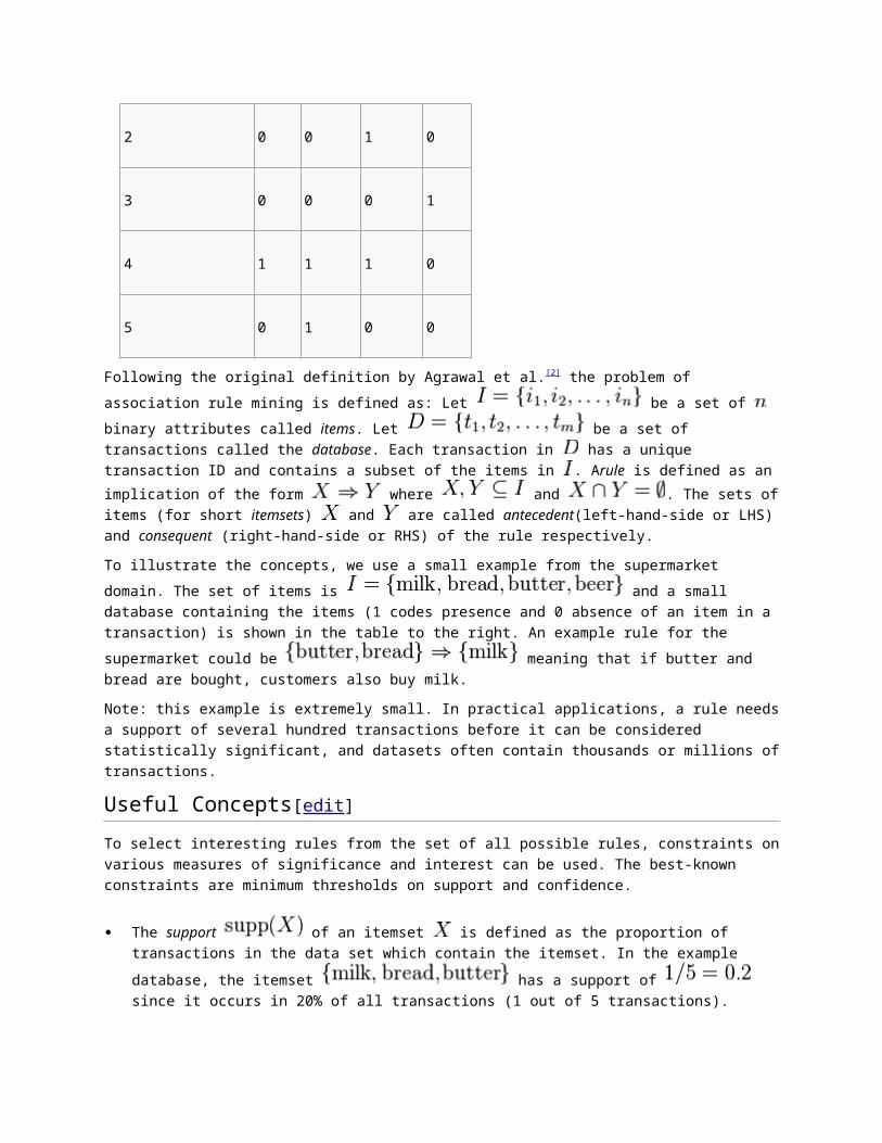
Definition[edit]

Example database with 4 items and 5 transactions

transaction ID milk bread butter beer

1 1 1 0 0

2 0 0 1 0

3 0 0 0 1

4 1 1 1 0

5 0 1 0 0

Following the original definition by Agrawal et al.[2] the problem of association rule mining is defined as:

Let   be a set of   binary attributes called items. Let   

be a set of transactions called the database. Each transaction in   has a unique transaction ID and

contains a subset of the items in  . Arule is defined as an implication of the form   

where   and  . The sets of items (for short itemsets)   and   are

called antecedent(left-hand-side or LHS) and consequent (right-hand-side or RHS) of the rule

respectively.

To illustrate the concepts, we use a small example from the supermarket domain. The set of items

is   and a small database containing the items (1 codes

presence and 0 absence of an item in a transaction) is shown in the table to the right. An example rule for

the supermarket could be   meaning that if butter and bread are

bought, customers also buy milk.

Note: this example is extremely small. In practical applications, a rule needs a support of several hundred

transactions before it can be considered statistically significant, and datasets often contain thousands or

millions of transactions.

Useful Concepts[edit]

To select interesting rules from the set of all possible rules, constraints on various measures of

significance and interest can be used. The best-known constraints are minimum thresholds on support

and confidence.

The support   of an itemset   is defined as the proportion of transactions in the data set

which contain the itemset. In the example database, the itemset   has a

support of   since it occurs in 20% of all transactions (1 out of 5 transactions).

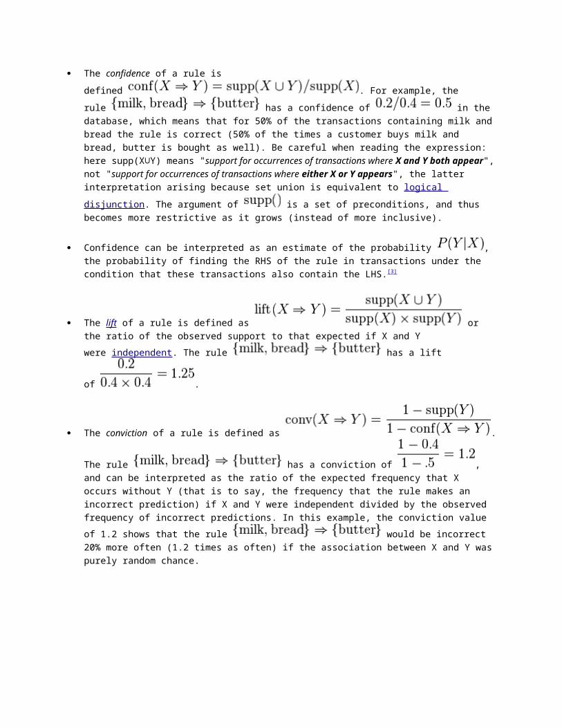
The confidence of a rule is defined  . For

example, the rule   has a confidence of   in the

database, which means that for 50% of the transactions containing milk and bread the rule is correct

(50% of the times a customer buys milk and bread, butter is bought as well). Be careful when reading

the expression: here supp(X∪Y) means "support for occurrences of transactions where X and Y both

appear", not "support for occurrences of transactions where either X or Y appears", the latter

interpretation arising because set union is equivalent to logical disjunction. The argument of   

is a set of preconditions, and thus becomes more restrictive as it grows (instead of more inclusive).

Confidence can be interpreted as an estimate of the probability  , the probability of finding

the RHS of the rule in transactions under the condition that these transactions also contain the LHS.[3]

The lift of a rule is defined as   or the ratio of the

observed support to that expected if X and Y were independent. The

rule   has a lift of  .

The conviction of a rule is defined as  . The

rule   has a conviction of  , and can be

interpreted as the ratio of the expected frequency that X occurs without Y (that is to say, the

frequency that the rule makes an incorrect prediction) if X and Y were independent divided by the

observed frequency of incorrect predictions. In this example, the conviction value of 1.2 shows that

the rule   would be incorrect 20% more often (1.2 times as often)

if the association between X and Y was purely random chance.

Process[edit]

Frequent itemset lattice, where the color of the box indicates how many transactions contain the combination of items. Note

that lower levels of the lattice can contain at most the minimum number of their parents' items; e.g. {ac} can have only at

most   items. This is called thedownward-closure property.[2]

Association rules are usually required to satisfy a user-specified minimum support and a user-specified

minimum confidence at the same time. Association rule generation is usually split up into two separate

steps:

1. First, minimum support is applied to find all frequent itemsets in a database.

2. Second, these frequent itemsets and the minimum confidence constraint are used to form rules.

While the second step is straightforward, the first step needs more attention.

Finding all frequent itemsets in a database is difficult since it involves searching all possible itemsets (item

combinations). The set of possible itemsets is the power set over   and has size   (excluding the

empty set which is not a valid itemset). Although the size of the powerset grows exponentially in the

number of items   in  , efficient search is possible using the downward-closure property of support[2]

[4] (also called anti-monotonicity[5]) which guarantees that for a frequent itemset, all its subsets are also

frequent and thus for an infrequent itemset, all its supersets must also be infrequent. Exploiting this

property, efficient algorithms (e.g., Apriori[6] and Eclat[7]) can find all frequent itemsets.

History[edit]

The concept of association rules was popularised particularly due to the 1993 article of Agrawal et al.,[2] which has acquired more than 6000 citations according to Google Scholar, as of March 2008, and is

thus one of the most cited papers in the Data Mining field. However, it is possible that what is now called

"association rules" is similar to what appears in the 1966 paper[8] on GUHA, a general data mining method

developed by Petr Hájek et al.[9]

Alternative measures of interestingness[edit]

Next to confidence also other measures of interestingness for rules were proposed. Some popular

measures are:

All-confidence[10]

Collective strength[11]

Conviction[12]

Leverage[13]

Lift (originally called interest)[14]

A definition of these measures can be found here. Several more measures are presented and compared

by Tan et al.[15] Looking for techniques that can model what the user has known (and using this models as

interestingness measures) is currently an active research trend under the name of "Subjective

Interestingness"

Statistically sound associations[edit]

One limitation of the standard approach to discovering associations is that by searching massive numbers

of possible associations to look for collections of items that appear to be associated, there is a large risk

of finding many spurious associations. These are collections of items that co-occur with unexpected

frequency in the data, but only do so by chance. For example, suppose we are considering a collection of

10,000 items and looking for rules containing two items in the left-hand-side and 1 item in the right-hand-

side. There are approximately 1,000,000,000,000 such rules. If we apply a statistical test for

independence with a significance level of 0.05 it means there is only a 5% chance of accepting a rule if

there is no association. If we assume there are no associations, we should nonetheless expect to find

50,000,000,000 rules. Statistically sound association discovery[16][17] controls this risk, in most cases

reducing the risk of finding any spurious associations to a user-specified significance level.

Algorithms[edit]

Many algorithms for generating association rules were presented over time.

Some well known algorithms are Apriori, Eclat and FP-Growth, but they only do half the job, since they

are algorithms for mining frequent itemsets. Another step needs to be done after to generate rules from

frequent itemsets found in a database.

Apriori algorithm[edit]

Main article: Apriori algorithm

Apriori[6] is the best-known algorithm to mine association rules. It uses a breadth-first search strategy to

count the support of itemsets and uses a candidate generation function which exploits the downward

closure property of support.

Eclat algorithm[edit]

Eclat[7] is a depth-first search algorithm using set intersection.

FP-growth algorithm[edit]

FP stands for frequent pattern.

In the first pass, the algorithm counts occurrence of items (attribute-value pairs) in the dataset, and stores

them to 'header table'. In the second pass, it builds the FP-tree structure by inserting instances. Items in

each instance have to be sorted by descending order of their frequency in the dataset, so that the tree

can be processed quickly. Items in each instance that do not meet minimum coverage threshold are

discarded. If many instances share most frequent items, FP-tree provides high compression close to tree

root.

Recursive processing of this compressed version of main dataset grows large item sets directly, instead

of generating candidate items and testing them against the entire database. Growth starts from the

bottom of the header table (having longest branches), by finding all instances matching given condition.

New tree is created, with counts projected from the original tree corresponding to the set of instances that

are conditional on the attribute, with each node getting sum of its children counts. Recursive growth ends

when no individual items conditional on the attribute meet minimum support threshold, and processing

continues on the remaining header items of the original FP-tree.

Once the recursive process has completed, all large item sets with minimum coverage have been found,

and association rule creation begins.

[18]

GUHA procedure ASSOC[edit]

GUHA is a general method for exploratory data analysis that has theoretical foundations in observational

calculi.[19]

The ASSOC procedure[20] is a GUHA method which mines for generalized association rules using

fast bitstrings operations. The association rules mined by this method are more general than those output

by apriori, for example "items" can be connected both with conjunction and disjunctions and the relation

between antecedent and consequent of the rule is not restricted to setting minimum support and

confidence as in apriori: an arbitrary combination of supported interest measures can be used.

OPUS search[edit]

OPUS is an efficient algorithm for rule discovery that, in contrast to most alternatives, does not require

either monotone or anti-monotone constraints such as minimum support.[21] Initially used to find rules for a

fixed consequent[21][22] it has subsequently been extended to find rules with any item as a consequent.[23] OPUS search is the core technology in the popular Magnum Opusassociation discovery system.

Lore[edit]

A famous story about association rule mining is the "beer and diaper" story. A purported survey of

behavior of supermarket shoppers discovered that customers (presumably young men) who buy diapers

tend also to buy beer. This anecdote became popular as an example of how unexpected association rules

might be found from everyday data. There are varying opinions as to how much of the story is true.[24] Daniel Powers says:[24]

In 1992, Thomas Blischok, manager of a retail consulting group at Teradata, and his staff prepared an

analysis of 1.2 million market baskets from about 25 Osco Drug stores. Database queries were developed

to identify affinities. The analysis "did discover that between 5:00 and 7:00 p.m. that consumers bought

beer and diapers". Osco managers did NOT exploit the beer and diapers relationship by moving the

products closer together on the shelves.

Other types of association mining[edit]

Contrast set learning is a form of associative learning. Contrast set learners use rules that differ

meaningfully in their distribution across subsets.[25]

Weighted class learning is another form of associative learning in which weight may be assigned to

classes to give focus to a particular issue of concern for the consumer of the data mining results.

High-order pattern discovery techniques facilitate the capture of high-order (polythetic) patterns or

event associations that are intrinsic to complex real-world data. [26]

K-optimal pattern discovery provides an alternative to the standard approach to association rule

learning that requires that each pattern appear frequently in the data.

Generalized Association Rules hierarchical taxonomy (concept hierarchy)

Quantitative Association Rules categorical and quantitative data [27]

Interval Data Association Rules e.g. partition the age into 5-year-increment ranged

Maximal Association Rules

Sequential pattern mining discovers subsequences that are common to more than minsup sequences

in a sequence database, where minsup is set by the user. A sequence is an ordered list of transactions.[28]

Sequential Rules discovering relationships between items while considering the time ordering. It is

generally applied on a sequence database. For example, a sequential rule found in database of

sequences of customer transactions can be that customers who bought a computer and CD-Roms, later

bought a webcam, with a given confidence and support.

See also[edit]

Sequence mining

Production system

Data miningFrom Wikipedia, the free encyclopedia

  (Redirected from Data Mining)

Not to be confused with analytics, information extraction, or data analysis.

Data mining (the analysis step of the "Knowledge Discovery in Databases" process, or KDD),[1] an

interdisciplinary subfield ofcomputer science,[2][3][4] is the computational process of discovering patterns in

large data sets involving methods at the intersection ofartificial intelligence, machine learning, statistics,

and database systems.[2] The overall goal of the data mining process is to extract information from a data set

and transform it into an understandable structure for further use.[2] Aside from the raw analysis step, it involves

database and data management aspects, data pre-processing, model and inference considerations,

interestingness metrics,complexity considerations, post-processing of discovered structures, visualization,

and online updating.[2]

The term is a buzzword,[5] and is frequently misused to mean any form of large-scale data or information

processing (collection,extraction, warehousing, analysis, and statistics) but is also generalized to any kind

of computer decision support system, includingartificial intelligence, machine learning, and business

intelligence. In the proper use of the word, the key term isdiscovery[citation needed], commonly defined as "detecting

something new". Even the popular book "Data mining: Practical machine learning tools and techniques with

Java"[6] (which covers mostly machine learning material) was originally to be named just "Practical machine

learning", and the term "data mining" was only added for marketing reasons.[7] Often the more general terms

"(large scale)data analysis", or "analytics" – or when referring to actual methods, artificial

intelligence and machine learning – are more appropriate.

The actual data mining task is the automatic or semi-automatic analysis of large quantities of data to extract

previously unknown interesting patterns such as groups of data records (cluster analysis), unusual records

(anomaly detection) and dependencies (association rule mining). This usually involves using database

techniques such as spatial indices. These patterns can then be seen as a kind of summary of the input data,

and may be used in further analysis or, for example, in machine learning and predictive analytics. For example,

the data mining step might identify multiple groups in the data, which can then be used to obtain more accurate

prediction results by a decision support system. Neither the data collection, data preparation, nor result

interpretation and reporting are part of the data mining step, but do belong to the overall KDD process as

additional steps.

The related terms data dredging, data fishing, and data snooping refer to the use of data mining methods to

sample parts of a larger population data set that are (or may be) too small for reliable statistical inferences to

be made about the validity of any patterns discovered. These methods can, however, be used in creating new

hypotheses to test against the larger data populations.

Data mining uses information from past data to analyze the outcome of a particular problem or situation that

may arise. Data mining works to analyze data stored in data warehouses that are used to store that data that is

being analyzed. That particular data may come from all parts of business, from the production to the

management. Managers also use data mining to decide upon marketing strategies for their product. They can

use data to compare and contrast among competitors. Data mining interprets its data into real time analysis

that can be used to increase sales, promote new product, or delete product that is not value-added to the

company.

Contents

  [hide] 

1     Etymology   

2     Background   

o 2.1      Research and evolution   

3     Process   

o 3.1      Pre-processing   

o 3.2      Data mining   

o 3.3      Results validation   

4     Standards   

5     Notable uses   

o 5.1      Games   

o 5.2      Business   

o 5.3      Science and engineering   

o 5.4      Human rights   

o 5.5      Medical data mining   

o 5.6      Spatial data mining   

o 5.7      Sensor data mining   

o 5.8      Visual data mining   

o 5.9      Music data mining   

o 5.10      Surveillance   

o 5.11      Pattern mining   

o 5.12      Subject-based data mining   

o 5.13      Knowledge grid   

6     Reliability / Validity   

7     Privacy concerns and ethics   

8     Software   

o 8.1      Free open-source data mining software and applications   

o 8.2      Commercial data-mining software and applications   

o 8.3      Marketplace surveys   

9     See also   

10      References   

11      Further reading   

12      External links   

Etymology[edit]

In the 1960s, statisticians used terms like "Data Fishing" or "Data Dredging" to refer to what they considered

the bad practice of analyzing data without an a-priori hypothesis. The term "Data Mining" appeared around

1990 in the database community. At the beginning of the century, there was a phrase "database mining"™,

trademarked by HNC, a San Diego-based company (now merged into FICO), to pitch their Data Mining

Workstation;[8] researchers consequently turned to "data mining". Other terms used include Data Archaeology,

Information Harvesting, Information Discovery, Knowledge Extraction, etc. Gregory Piatetsky-Shapiro coined

the term "Knowledge Discovery in Databases" for the first workshop on the same topic (1989) and this term

became more popular in AI and Machine Learning Community. However, the term data mining became more

popular in the business and press communities.[9]Currently, Data Mining and Knowledge Discovery are used

interchangeably.

Background[edit]

The manual extraction of patterns from data has occurred for centuries. Early methods of identifying patterns in

data include Bayes' theorem (1700s) and regression analysis (1800s). The proliferation, ubiquity and

increasing power of computer technology has dramatically increased data collection, storage, and manipulation

ability. As data sets have grown in size and complexity, direct "hands-on" data analysis has increasingly been

augmented with indirect, automated data processing, aided by other discoveries in computer science, such

as neural networks, cluster analysis, genetic algorithms (1950s), decision trees (1960s), and support vector

machines (1990s). Data mining is the process of applying these methods with the intention of uncovering

hidden patterns[10] in large data sets. It bridges the gap from applied statistics and artificial intelligence (which

usually provide the mathematical background) to database management by exploiting the way data is stored

and indexed in databases to execute the actual learning and discovery algorithms more efficiently, allowing

such methods to be applied to ever larger data sets.

Research and evolution[edit]

The premier professional body in the field is the Association for Computing Machinery's (ACM) Special Interest

Group (SIG) onKnowledge Discovery and Data Mining (SIGKDD). Since 1989 this ACM SIG has hosted an

annual international conference and published its proceedings,[11] and since 1999 it has published a

biannual academic journal titled "SIGKDD Explorations".[12]

Computer science conferences on data mining include:

CIKM Conference  – ACM Conference on Information and Knowledge Management

DMIN Conference  – International Conference on Data Mining

DMKD Conference  – Research Issues on Data Mining and Knowledge Discovery

ECDM Conference  – European Conference on Data Mining

ECML-PKDD Conference  – European Conference on Machine Learning and Principles and Practice of

Knowledge Discovery in Databases

EDM Conference  – International Conference on Educational Data Mining

ICDM Conference  – IEEE International Conference on Data Mining

KDD Conference  – ACM SIGKDD Conference on Knowledge Discovery and Data Mining

MLDM Conference  – Machine Learning and Data Mining in Pattern Recognition

PAKDD Conference  – The annual Pacific-Asia Conference on Knowledge Discovery and Data Mining

PAW Conference  – Predictive Analytics World

SDM Conference  – SIAM International Conference on Data Mining (SIAM)

SSTD Symposium  – Symposium on Spatial and Temporal Databases

WSDM Conference  – ACM Conference on Web Search and Data Mining

Data mining topics are also present on many data management/database conferences such as the ICDE

Conference, SIGMOD Conference and International Conference on Very Large Data Bases

Process[edit]

The Knowledge Discovery in Databases (KDD) process is commonly defined with the stages:

(1) Selection

(2) Pre-processing

(3) Transformation

(4) Data Mining

(5) Interpretation/Evaluation.[1]

It exists, however, in many variations on this theme, such as the Cross Industry

Standard Process for Data Mining (CRISP-DM) which defines six phases:

(1) Business Understanding

(2) Data Understanding

(3) Data Preparation

(4) Modeling

(5) Evaluation

(6) Deployment

or a simplified process such as (1) pre-processing, (2) data

mining, and (3) results validation.

Polls conducted in 2002, 2004, and 2007 show that the

CRISP-DM methodology is the leading methodology used by

data miners.[13][14][15] The only other data mining standard

named in these polls was SEMMA. However, 3-4 times as

many people reported using CRISP-DM. Several teams of

researchers have published reviews of data mining process

models,[16][17] and Azevedo and Santos conducted a

comparison of CRISP-DM and SEMMA in 2008.[18]

Pre-processing[edit]

Before data mining algorithms can be used, a target data set

must be assembled. As data mining can only uncover

patterns actually present in the data, the target data set must

be large enough to contain these patterns while remaining

concise enough to be mined within an acceptable time limit.

A common source for data is a data mart or data warehouse.

Pre-processing is essential to analyze the multivariate data

sets before data mining. The target set is then cleaned. Data

cleaning removes the observations containing noiseand

those with missing data.

Data mining[edit]

Data mining involves six common classes of tasks:[1]

Anomaly detection  (Outlier/change/deviation detection)

– The identification of unusual data records, that might

be interesting or data errors that require further

investigation.

Association rule learning  (Dependency modeling) –

Searches for relationships between variables. For

example a supermarket might gather data on customer

purchasing habits. Using association rule learning, the

supermarket can determine which products are

frequently bought together and use this information for

marketing purposes. This is sometimes referred to as

market basket analysis.

Clustering  – is the task of discovering groups and

structures in the data that are in some way or another

"similar", without using known structures in the data.

Classification  – is the task of generalizing known

structure to apply to new data. For example, an e-mail

program might attempt to classify an e-mail as

"legitimate" or as "spam".

Regression  – Attempts to find a function which models

the data with the least error.

Summarization  – providing a more compact

representation of the data set, including visualization

and report generation.

Sequential pattern mining  – Sequential pattern mining

finds sets of data items that occur together frequently in

some sequences. Sequential pattern mining, which

extracts frequent subsequences from a sequence

database, has attracted a great deal of interest during

the recent data mining research because it is the basis

of many applications, such as: web user analysis, stock

trend prediction, DNA sequence analysis, finding

language or linguistic patterns from natural language

texts, and using the history of symptoms to predict

certain kind of disease.

Results validation[edit]

This section is missing information about non-classification tasks in data mining. It only covers machine learning. This concern has been noted on the talk page where whether or not 

to include such information may be discussed. (September 2011)

The final step of knowledge discovery from data is to verify

that the patterns produced by the data mining algorithms

occur in the wider data set. Not all patterns found by the data

mining algorithms are necessarily valid. It is common for the

data mining algorithms to find patterns in the training set

which are not present in the general data set. This is

called overfitting. To overcome this, the evaluation uses

a test set of data on which the data mining algorithm was not

trained. The learned patterns are applied to this test set and

the resulting output is compared to the desired output. For

example, a data mining algorithm trying to distinguish "spam"

from "legitimate" emails would be trained on a training set of

sample e-mails. Once trained, the learned patterns would be

applied to the test set of e-mails on which it had not been

trained. The accuracy of the patterns can then be measured

from how many e-mails they correctly classify. A number of

statistical methods may be used to evaluate the algorithm,

such as ROC curves.

If the learned patterns do not meet the desired standards,

then it is necessary to re-evaluate and change the pre-

processing and data mining steps. If the learned patterns do

meet the desired standards, then the final step is to interpret

the learned patterns and turn them into knowledge.

Standards[edit]

There have been some efforts to define standards for the

data mining process, for example the 1999 European Cross

Industry Standard Process for Data Mining (CRISP-DM 1.0)

and the 2004 Java Data Mining standard (JDM 1.0).

Development on successors to these processes (CRISP-DM

2.0 and JDM 2.0) was active in 2006, but has stalled since.

JDM 2.0 was withdrawn without reaching a final draft.

For exchanging the extracted models – in particular for use

in predictive analytics – the key standard is the Predictive

Model Markup Language (PMML), which is an XML-based

language developed by the Data Mining Group (DMG) and

supported as exchange format by many data mining

applications. As the name suggests, it only covers prediction

models, a particular data mining task of high importance to

business applications. However, extensions to cover (for

example) subspace clustering have been proposed

independently of the DMG.[19]

Notable uses[edit]

See also category: Applied data mining

Games[edit]

Since the early 1960s, with the availability of oracles for

certain combinatorial games, also called tablebases (e.g. for

3x3-chess) with any beginning configuration, small-

board dots-and-boxes, small-board-hex, and certain

endgames in chess, dots-and-boxes, and hex; a new area

for data mining has been opened. This is the extraction of

human-usable strategies from these oracles. Current pattern

recognition approaches do not seem to fully acquire the high

level of abstraction required to be applied successfully.

Instead, extensive experimentation with the tablebases –

combined with an intensive study of tablebase-answers to

well designed problems, and with knowledge of prior art (i.e.

pre-tablebase knowledge) – is used to yield insightful

patterns. Berlekamp (in dots-and-boxes, etc.) and John

Nunn (in chess endgames) are notable examples of

researchers doing this work, though they were not – and are

not – involved in tablebase generation.

Business[edit]

Data mining is the analysis of historical business activities,

stored as static data in data warehouse databases, to reveal

hidden patterns and trends. Data mining software uses

advanced pattern recognition algorithms to sift through large

amounts of data to assist in discovering previously unknown

strategic business information. Examples of what businesses

use data mining for include performing market analysis to

identify new product bundles, finding the root cause of

manufacturing problems, to prevent customer attrition and

acquire new customers, cross-sell to existing customers, and

profile customers with more accuracy.[20] In today’s world raw

data is being collected by companies at an exploding rate.

For example, Walmart processes over 20 million point-of-

sale transactions every day. This information is stored in a

centralized database, but would be useless without some

type of data mining software to analyse it. If Walmart

analyzed their point-of-sale data with data mining techniques

they would be able to determine sales trends, develop

marketing campaigns, and more accurately predict customer

loyalty.[21] Every time we use our credit card, a store loyalty

card, or fill out a warranty card data is being collected about

our purchasing behavior. Many people find the amount of

information stored about us from companies, such as

Google, Facebook, and Amazon, disturbing and are

concerned about privacy. Although there is the potential for

our personal data to be used in harmful, or unwanted, ways

it is also being used to make our lives better. For example,

Ford and Audi hope to one day collect information about

customer driving patterns so they can recommend safer

routes and warn drivers about dangerous road conditions.[22]

Data mining in customer relationship

management applications can contribute significantly to the

bottom line.[citation needed] Rather than randomly contacting a

prospect or customer through a call center or sending mail, a

company can concentrate its efforts on prospects that are

predicted to have a high likelihood of responding to an offer.

More sophisticated methods may be used to optimize

resources across campaigns so that one may predict to

which channel and to which offer an individual is most likely

to respond (across all potential offers). Additionally,

sophisticated applications could be used to automate

mailing. Once the results from data mining (potential

prospect/customer and channel/offer) are determined, this

"sophisticated application" can either automatically send an

e-mail or a regular mail. Finally, in cases where many people

will take an action without an offer, "uplift modeling" can be

used to determine which people have the greatest increase

in response if given an offer. Uplift modeling thereby enables

marketers to focus mailings and offers on persuadable

people, and not to send offers to people who will buy the

product without an offer. Data clusteringcan also be used to

automatically discover the segments or groups within a

customer data set.

Businesses employing data mining may see a return on

investment, but also they recognize that the number of

predictive models can quickly become very large. Rather

than using one model to predict how many customers

will churn, a business could build a separate model for each

region and customer type. Then, instead of sending an offer

to all people that are likely to churn, it may only want to send

offers to loyal customers. Finally, the business may want to

determine which customers are going to be profitable over a

certain window in time, and only send the offers to those that

are likely to be profitable. In order to maintain this quantity of

models, they need to manage model versions and move on

to automated data mining.

Data mining can also be helpful to human resources (HR)

departments in identifying the characteristics of their most

successful employees. Information obtained – such as

universities attended by highly successful employees – can

help HR focus recruiting efforts accordingly. Additionally,

Strategic Enterprise Management applications help a

company translate corporate-level goals, such as profit and

margin share targets, into operational decisions, such as

production plans and workforce levels.[23]

Another example of data mining, often called the market

basket analysis, relates to its use in retail sales. If a clothing

store records the purchases of customers, a data mining

system could identify those customers who favor silk shirts

over cotton ones. Although some explanations of

relationships may be difficult, taking advantage of it is easier.

The example deals with association rules within transaction-

based data. Not all data are transaction based and logical, or

inexact rules may also be present within a database.

Market basket analysis has also been used to identify the

purchase patterns of the Alpha Consumer. Alpha Consumers

are people that play a key role in connecting with the

concept behind a product, then adopting that product, and

finally validating it for the rest of society. Analyzing the data

collected on this type of user has allowed companies to

predict future buying trends and forecast supply demands.

[citation needed]

Data mining is a highly effective tool in the catalog marketing

industry.[citation needed] Catalogers have a rich database of

history of their customer transactions for millions of

customers dating back a number of years. Data mining tools

can identify patterns among customers and help identify the

most likely customers to respond to upcoming mailing

campaigns.

Data mining for business applications is a component that

needs to be integrated into a complex modeling and decision

making process. Reactive business intelligence (RBI)

advocates a "holistic" approach that integrates data

mining, modeling, and interactive visualization into an end-

to-end discovery and continuous innovation process

powered by human and automated learning.[24]

In the area of decision making, the RBI approach has been

used to mine knowledge that is progressively acquired from

the decision maker, and then self-tune the decision method

accordingly.[25]

An example of data mining related to an integrated-circuit

(IC) production line is described in the paper "Mining IC Test

Data to Optimize VLSI Testing."[26] In this paper, the

application of data mining and decision analysis to the

problem of die-level functional testing is described.

Experiments mentioned demonstrate the ability to apply a

system of mining historical die-test data to create a

probabilistic model of patterns of die failure. These patterns

are then utilized to decide, in real time, which die to test next

and when to stop testing. This system has been shown,

based on experiments with historical test data, to have the

potential to improve profits on mature IC products.

Science and engineering[edit]

In recent years, data mining has been used widely in the

areas of science and engineering, such

as bioinformatics, genetics, medicine,education and electrica

l power engineering.

In the study of human genetics, sequence mining helps

address the important goal of understanding the mapping

relationship between the inter-individual variations in

human DNA sequence and the variability in disease

susceptibility. In simple terms, it aims to find out how the

changes in an individual's DNA sequence affects the risks of

developing common diseases such as cancer, which is of

great importance to improving methods of diagnosing,

preventing, and treating these diseases. The data mining

method that is used to perform this task is known

as multifactor dimensionality reduction.[27]

In the area of electrical power engineering, data mining

methods have been widely used for condition monitoring of

high voltage electrical equipment. The purpose of condition

monitoring is to obtain valuable information on, for example,

the status of the insulation(or other important safety-related

parameters). Data clustering techniques – such as the self-

organizing map (SOM), have been applied to vibration

monitoring and analysis of transformer on-load tap-changers

(OLTCS). Using vibration monitoring, it can be observed that

each tap change operation generates a signal that contains

information about the condition of the tap changer contacts

and the drive mechanisms. Obviously, different tap positions

will generate different signals. However, there was

considerable variability amongst normal condition signals for

exactly the same tap position. SOM has been applied to

detect abnormal conditions and to hypothesize about the

nature of the abnormalities.[28]

Data mining methods have also been applied to dissolved

gas analysis (DGA) in power transformers. DGA, as a

diagnostics for power transformers, has been available for

many years. Methods such as SOM has been applied to

analyze generated data and to determine trends which are

not obvious to the standard DGA ratio methods (such as

Duval Triangle).[28]

Another example of data mining in science and engineering

is found in educational research, where data mining has

been used to study the factors leading students to choose to

engage in behaviors which reduce their learning,[29] and to

understand factors influencing university student retention.

[30] A similar example of social application of data mining is its

use in expertise finding systems, whereby descriptors of

human expertise are extracted, normalized, and classified so

as to facilitate the finding of experts, particularly in scientific

and technical fields. In this way, data mining can

facilitate institutional memory.

Other examples of application of data mining methods

are biomedical data facilitated by domain ontologies,

[31] mining clinical trial data,[32] and traffic analysis using SOM.

[33]

In adverse drug reaction surveillance, the Uppsala

Monitoring Centre has, since 1998, used data mining

methods to routinely screen for reporting patterns indicative

of emerging drug safety issues in the WHO global database

of 4.6 million suspected adverse drug reactionincidents.

[34] Recently, similar methodology has been developed to

mine large collections of electronic health records for

temporal patterns associating drug prescriptions to medical

diagnoses.[35]

Data mining has been applied software artifacts within the

realm of software engineering: Mining Software Repositories.

Human rights[edit]

Data mining of government records – particularly records of

the justice system (i.e. courts, prisons) – enables the

discovery of systemic human rights violations in connection

to generation and publication of invalid or fraudulent legal

records by various government agencies.[36][37]

Medical data mining[edit]

In 2011, the case of Sorrell v. IMS Health, Inc., decided by

the Supreme Court of the United States, ruled

that pharmacies may share information with outside

companies. This practice was authorized under the 1st

Amendment of the Constitution, protecting the "freedom of

speech."[38]

Spatial data mining[edit]

Spatial data mining is the application of data mining methods

to spatial data. The end objective of spatial data mining is to

find patterns in data with respect to geography. So far, data

mining and Geographic Information Systems (GIS) have

existed as two separate technologies, each with its own

methods, traditions, and approaches to visualization and

data analysis. Particularly, most contemporary GIS have only

very basic spatial analysis functionality. The immense

explosion in geographically referenced data occasioned by

developments in IT, digital mapping, remote sensing, and the

global diffusion of GIS emphasizes the importance of

developing data-driven inductive approaches to geographical

analysis and modeling.

Data mining offers great potential benefits for GIS-based

applied decision-making. Recently, the task of integrating

these two technologies has become of critical importance,

especially as various public and private sector organizations

possessing huge databases with thematic and

geographically referenced data begin to realize the huge

potential of the information contained therein. Among those

organizations are:

offices requiring analysis or dissemination of geo-

referenced statistical data

public health services searching for explanations of

disease clustering

environmental agencies assessing the impact of

changing land-use patterns on climate change

geo-marketing companies doing customer segmentation

based on spatial location.

Challenges in Spatial mining: Geospatial data repositories

tend to be very large. Moreover, existing GIS datasets are

often splintered into feature and attribute components that

are conventionally archived in hybrid data management

systems. Algorithmic requirements differ substantially for

relational (attribute) data management and for topological

(feature) data management.[39] Related to this is the range

and diversity of geographic data formats, which present

unique challenges. The digital geographic data revolution is

creating new types of data formats beyond the traditional

"vector" and "raster" formats. Geographic data repositories

increasingly include ill-structured data, such as imagery and

geo-referenced multi-media.[40]

There are several critical research challenges in geographic

knowledge discovery and data mining. Miller and Han[41] offer

the following list of emerging research topics in the field:

Developing and supporting geographic data

warehouses (GDW's): Spatial properties are often

reduced to simple aspatialattributes in mainstream data

warehouses. Creating an integrated GDW requires

solving issues of spatial and temporal data

interoperability – including differences in semantics,

referencing systems, geometry, accuracy, and position.

Better spatio-temporal representations in

geographic knowledge discovery: Current geographic

knowledge discovery (GKD) methods generally use very

simple representations of geographic objects and spatial

relationships. Geographic data mining methods should

recognize more complex geographic objects (i.e. lines

and polygons) and relationships (i.e. non-Euclidean

distances, direction, connectivity, and interaction

through attributed geographic space such as terrain).

Furthermore, the time dimension needs to be more fully

integrated into these geographic representations and

relationships.

Geographic knowledge discovery using diverse data

types: GKD methods should be developed that can

handle diverse data types beyond the traditional raster

and vector models, including imagery and geo-

referenced multimedia, as well as dynamic data types

(video streams, animation).

Sensor data mining[edit]

Wireless sensor networks can be used for facilitating the

collection of data for spatial data mining for a variety of

applications such as air pollution monitoring.[42] A

characteristic of such networks is that nearby sensor nodes

monitoring an environmental feature typically register similar

values. This kind of data redundancy due to the spatial

correlation between sensor observations inspires the

techniques for in-network data aggregation and mining. By

measuring the spatial correlation between data sampled by

different sensors, a wide class of specialized algorithms can

be developed to develop more efficient spatial data mining

algorithms.[43]

Visual data mining[edit]

In the process of turning from analogical into digital, large

data sets have been generated, collected, and stored

discovering statistical patterns, trends and information which

is hidden in data, in order to build predictive patterns.

Studies suggest visual data mining is faster and much more

intuitive than is traditional data mining.[44][45][46] See

also Computer vision.

Music data mining[edit]

Data mining techniques, and in particular co-

occurrence analysis, has been used to discover relevant

similarities among music corpora (radio lists, CD databases)

for the purpose of classifying music into genres in a more

objective manner.[47]

Surveillance[edit]

Data mining has been used to stop terrorist programs under

the U.S. government, including the Total Information

Awareness (TIA) program, Secure Flight (formerly known as

Computer-Assisted Passenger Prescreening System

(CAPPS II)), Analysis, Dissemination, Visualization, Insight,

Semantic Enhancement (ADVISE),[48] and the Multi-state

Anti-Terrorism Information Exchange (MATRIX).[49]These

programs have been discontinued due to controversy over

whether they violate the 4th Amendment to the United States

Constitution, although many programs that were formed

under them continue to be funded by different organizations

or under different names.[50]

In the context of combating terrorism, two particularly

plausible methods of data mining are "pattern mining" and

"subject-based data mining".

Pattern mining[edit]

"Pattern mining" is a data mining method that involves

finding existing patterns in data. In this context patterns often

meansassociation rules. The original motivation for

searching association rules came from the desire to analyze

supermarket transaction data, that is, to examine customer

behavior in terms of the purchased products. For example,

an association rule "beer ⇒ potato chips (80%)" states that

four out of five customers that bought beer also bought

potato chips.

In the context of pattern mining as a tool to identify terrorist

activity, the National Research Council provides the following

definition: "Pattern-based data mining looks for patterns

(including anomalous data patterns) that might be associated

with terrorist activity — these patterns might be regarded as

small signals in a large ocean of noise."[51][52][53] Pattern

Mining includes new areas such aMusic Information

Retrieval (MIR) where patterns seen both in the temporal

and non temporal domains are imported to classical

knowledge discovery search methods.

Subject-based data mining[edit]

"Subject-based data mining" is a data mining method

involving the search for associations between individuals in

data. In the context of combating terrorism, the National

Research Council provides the following definition: "Subject-

based data mining uses an initiating individual or other

datum that is considered, based on other information, to be

of high interest, and the goal is to determine what other

persons or financial transactions or movements, etc., are

related to that initiating datum."[52]

Knowledge grid[edit]

Knowledge discovery "On the Grid" generally refers to

conducting knowledge discovery in an open environment

using grid computingconcepts, allowing users to integrate

data from various online data sources, as well make use of

remote resources, for executing their data mining tasks. The

earliest example was the Discovery Net,[54][55] developed

at Imperial College London, which won the "Most Innovative

Data-Intensive Application Award" at the ACM SC02

(Supercomputing 2002) conference and exhibition, based on

a demonstration of a fully interactive distributed knowledge

discovery application for a bioinformatics application. Other

examples include work conducted by researchers at

the University of Calabria, who developed a Knowledge Grid

architecture for distributed knowledge discovery, based

on grid computing.[56][57]

Reliability / Validity[edit]

Data mining can be misused, and can also unintentionally

produce results which appear significant but which do not

actually predict future behavior and cannot be reproduced on

a new sample of data. See Data dredging.

Privacy concerns and ethics[edit]

Some people believe that data mining itself is ethically

neutral.[58] While the term "data mining" has no ethical

implications, it is often associated with the mining of

information in relation to peoples' behavior (ethical and

otherwise). To be precise, data mining is a statistical method

that is applied to a set of information (i.e. a data set).

Associating these data sets with people is an extreme

narrowing of the types of data that are available. Examples

could range from a set of crash test data for passenger

vehicles, to the performance of a group of stocks. These

types of data sets make up a great proportion of the

information available to be acted on by data mining methods,

and rarely have ethical concerns associated with them.

However, the ways in which data mining can be used can in

some cases and contexts raise questions regarding privacy,

legality, and ethics.[59] In particular, data mining government

or commercial data sets for national security or law

enforcement purposes, such as in the Total Information

Awareness Program or inADVISE, has raised privacy

concerns.[60][61]

Data mining requires data preparation which can uncover

information or patterns which may compromise

confidentiality and privacy obligations. A common way for

this to occur is through data aggregation. Data aggregation

involves combining data together (possibly from various

sources) in a way that facilitates analysis (but that also might

make identification of private, individual-level data deducible

or otherwise apparent).[62] This is not data mining per se, but

a result of the preparation of data before – and for the

purposes of – the analysis. The threat to an individual's

privacy comes into play when the data, once compiled,

cause the data miner, or anyone who has access to the

newly compiled data set, to be able to identify specific

individuals, especially when the data were originally

anonymous.

It is recommended that an individual is made aware of the

following before data are collected:[62]

the purpose of the data collection and any (known) data

mining projects

how the data will be used

who will be able to mine the data and use the data and

their derivatives

the status of security surrounding access to the data

how collected data can be updated.

In America, privacy concerns have been addressed to some

extent by the US Congress via the passage of regulatory

controls such as the Health Insurance Portability and

Accountability Act (HIPAA). The HIPAA requires individuals

to give their "informed consent" regarding information they

provide and its intended present and future uses. According

to an article in Biotech Business Week', "'[i]n practice, HIPAA

may not offer any greater protection than the longstanding

regulations in the research arena,' says the AAHC. More

importantly, the rule's goal of protection through informed

consent is undermined by the complexity of consent forms

that are required of patients and participants, which

approach a level of incomprehensibility to average

individuals."[63] This underscores the necessity for data

anonymity in data aggregation and mining practices.

Data may also be modified so as to become anonymous, so

that individuals may not readily be identified.[62] However,

even "de-identified"/"anonymized" data sets can potentially

contain enough information to allow identification of

individuals, as occurred when journalists were able to find

several individuals based on a set of search histories that

were inadvertently released by AOL.[64]

Software

Educational data mining

Educational Data Mining (EDM) describes a research field concerned with the application of data

mining to information generated as a consequence of students interacting with computer-based learning

environments (e.g., intelligent tutoring systems). At a high level, the field seeks to develop methods for

exploring these interaction traces in order to understand how people learn in the context of such systems.[1] A key area of EDM is mining computer logs of student performance.[2] Another key area is mining

enrollment data.[3] Key uses of EDM include predicting student performance, and studying learning in

order to recommend improvements to current educational practice. EDM can be considered one of

the learning sciences, as well as an area of data mining. A related field is learning analytics.

Contents

  [hide] 

1   EDM methods

2   Classifiers for EDM

3   Process Mining from Educational Data

4   Applications

5   Publication Venues

6   The use of Educational Data Mining in the KDD Cup

7   References

EDM methods[edit]

The types of EDM method are related to those found in data mining in general, but with some differences

based on the unique features of educational data.

Ryan Baker [4] classifies the areas of EDM as follows:

Prediction

Classification

Regression

Density estimation

Clustering

Relationship mining

Association rule mining

Correlation mining

Sequential pattern mining

Causal data mining

Distillation of data for human judgment

Discovery with models

Baker and Kalina Yacef claim that discovery with models is particularly prominent in EDM, as compared

to data mining in general. In discovery with models, a model of a phenomenon is developed through any

process that can be validated in some fashion (most commonly, prediction or knowledge engineering),

and this model is then used as a component in another analysis, such as prediction or relationship

mining.

Classifiers for EDM[edit]

Classification has many applications in modern educational technology. Here are lists of main principles

and classification approaches used in EDM.[5]

Main Principles

Discriminative or Probabilistic Classifier

Classification Accuracy

Overfitting

Linear and Nonlinear Class Boundaries

Data Preprocessing

Classification Approaches

Decision Trees

Bayesian Classifiers

Neural Networks

K-Nearest Neighbor Classifiers

Support Vector Machines

Linear Regression

Comparison

Process Mining from Educational Data[edit]

The following is the process of mining educational data.[6]

Process mining consists of three subfields:

Conformance checking

Model discovery

Model extension ( For example: ProM framework.)

Process Mining Educational Data Set:

Data Preparation

Visual Mining with Dotted Chart Analysis

Conformance Analysis

Conformance Checking

LTL Analysis

Process Discovery with Fuzzy Miner

Applications[edit]

A list of the primary applications of EDM is provided by Cristobal Romero and Sebastian Ventura.[7] In

their taxonomy, the areas of EDM application are:

Analysis and visualization of data

Providing feedback for supporting instructors

Recommendations for students

Predicting student performance

Student modeling

Detecting undesirable student behaviors

Grouping students

Social network analysis

Developing concept maps

Constructing courseware

Planning and scheduling

Statistical classificationIn machine learning and statistics, classification is the problem of identifying to which of a set

of categories (sub-populations) a new observation belongs, on the basis of a training set of data

containing observations (or instances) whose category membership is known. The individual observations

are analyzed into a set of quantifiable properties, known as various explanatory variables, features, etc.

These properties may variously be categorical (e.g. "A", "B", "AB" or "O", for blood type), ordinal (e.g.

"large", "medium" or "small"),integer-valued (e.g. the number of occurrences of a part word in an email)

or real-valued (e.g. a measurement of blood pressure). Some algorithms work only in terms of discrete

data and require that real-valued or integer-valued data be discretized into groups (e.g. less than 5,

between 5 and 10, or greater than 10). An example would be assigning a given email into "spam" or "non-

spam" classes or assigning a diagnosis to a given patient as described by observed characteristics of the

patient (gender, blood pressure, presence or absence of certain symptoms, etc.).

An algorithm that implements classification, especially in a concrete implementation, is known as

a classifier. The term "classifier" sometimes also refers to the mathematical function, implemented by a

classification algorithm, that maps input data to a category.

In the terminology of machine learning, classification is considered an instance of supervised learning, i.e.

learning where a training set of correctly-identified observations is available. The

corresponding unsupervised procedure is known as clustering (or cluster analysis), and involves grouping

data into categories based on some measure of inherent similarity (e.g. the distance between instances,

considered as vectors in a multi-dimensional vector space).

Terminology across fields is quite varied. In statistics, where classification is often done with logistic

regression or a similar procedure, the properties of observations are termed explanatory

variables (or independent variables, regressors, etc.), and the categories to be predicted are known as

outcomes, which are considered to be possible values of the dependent variable. In machine learning, the

observations are often known as instances, the explanatory variables are termed features (grouped into

a feature vector), and the possible categories to be predicted are classes. There is also some argument

over whether classification methods that do not involve astatistical model can be considered "statistical".

Other fields may use different terminology: e.g. in community ecology, the term "classification" normally

refers to cluster analysis, i.e. a type of unsupervised learning, rather than the supervised learning

described in this article.

Contents

  [hide] 

1   Relation to other problems

2   Frequentist procedures

3   Bayesian procedures

4   Binary and multiclass classification

5   Feature vectors

6   Linear classifiers

7   Algorithms

8   Evaluation

9   Application domains

10   See also

11   References

12   External links

Relation to other problems[edit]

Classification and clustering are examples of the more general problem of pattern recognition, which is

the assignment of some sort of output value to a given input value. Other examples are regression, which

assigns a real-valued output to each input; sequence labeling, which assigns a class to each member of a

sequence of values (for example, part of speech tagging, which assigns a part of speech to each word in

an input sentence); parsing, which assigns a parse tree to an input sentence, describing the syntactic

structure of the sentence; etc.

A common subclass of classification is probabilistic classification. Algorithms of this nature

use statistical inference to find the best class for a given instance. Unlike other algorithms, which simply

output a "best" class, probabilistic algorithms output a probability of the instance being a member of each

of the possible classes. The best class is normally then selected as the one with the highest probability.

However, such an algorithm has numerous advantages over non-probabilistic classifiers:

It can output a confidence value associated with its choice (in general, a classifier that can do this is

known as a confidence-weighted classifier)

Correspondingly, it can abstain when its confidence of choosing any particular output is too low

Because of the probabilities output, probabilistic classifiers can be more effectively incorporated into

larger machine-learning tasks, in a way that partially or completely avoids the problem of error

propagation.

Frequentist procedures[edit]

Early work on statistical classification was undertaken by Fisher,[1][2] in the context of two-group problems,

leading to Fisher's linear discriminant function as the rule for assigning a group to a new observation.[3] This early work assumed that data-values within each of the two groups had a multivariate normal

distribution. The extension of this same context to more than two-groups has also been considered with a

restriction imposed that the classification rule should be linear.[3][4] Later work for the multivariate normal

distribution allowed the classifier to be nonlinear:[5] several classification rules can be derived based on

slight different adjustments of theMahalanobis distance, with a new observation being assigned to the

group whose centre has the lowest adjusted distance from the observation.

Bayesian procedures[edit]

Unlike frequentist procedures, Bayesian classification procedures provide a natural way of taking into

account any available information about the relative sizes of the sub-populations associated with the

different groups within the overall population.[6] Bayesian procedures tend to be computationally

expensive and, in the days before Markov chain Monte Carlo computations were developed,

approximations for Bayesian clustering rules were devised.[7]

Some Bayesian procedures involve the calculation of group membership probabilities: these can be

viewed as providing a more informative outcome of a data analysis than a simple attribution of a single

group-label to each new observation.

Binary and multiclass classification[edit]

Classification can be thought of as two separate problems - binary classification and multiclass

classification. In binary classification, a better understood task, only two classes are involved, whereas

multiclass classification involves assigning an object to one of several classes.[8] Since many classification

methods have been developed specifically for binary classification, multiclass classification often requires

the combined use of multiple binary classifiers.

Feature vectors[edit]

Most algorithms describe an individual instance whose category is to be predicted using a feature

vector of individual, measurable properties of the instance. Each property is termed a feature, also known

in statistics as an explanatory variable (or independent variable, although in general different features

may or may not be statistically independent). Features may variously be binary ("male" or

"female"); categorical (e.g. "A", "B", "AB" or "O", for blood type); ordinal (e.g. "large", "medium" or

"small"); integer-valued (e.g. the number of occurrences of a particular word in an email); or real-

valued (e.g. a measurement of blood pressure). If the instance is an image, the feature values might

correspond to the pixels of an image; if the instance is a piece of text, the feature values might be

occurrence frequencies of different words. Some algorithms work only in terms of discrete data and

require that real-valued or integer-valued data be discretized into groups (e.g. less than 5, between 5 and

10, or greater than 10).

The vector space associated with these vectors is often called the feature space. In order to reduce the

dimensionality of the feature space, a number of dimensionality reduction techniques can be employed.

Linear classifiers[edit]

A large number of algorithms for classification can be phrased in terms of a linear function that assigns a

score to each possible category k by combining the feature vector of an instance with a vector of weights,

using a dot product. The predicted category is the one with the highest score. This type of score function

is known as a linear predictor function and has the following general form:

where Xi is the feature vector for instance i, βk is the vector of weights corresponding to category k,

and score(Xi, k) is the score associated with assigning instance i to category k. In discrete

choice theory, where instances represent people and categories represent choices, the score is

considered the utility associated with person i choosing category k.

Algorithms with this basic setup are known as linear classifiers. What distinguishes them is the

procedure for determining (training) the optimal weights/coefficients and the way that the score is

interpreted.

Examples of such algorithms are

Logistic regression  and multinomial logit

Probit regression

The perceptron algorithm

Support vector machines

Linear discriminant analysis .

Algorithms[edit]

This article is in a list format that may be better presented using prose. You

can help by converting this article to prose, if appropriate. Editing help is

available. (May 2012)

The most widely used classifiers are the neural network (multi-layer perceptron), support vector

machines, k-nearest neighbours, Gaussian mixture model, Gaussian, naive Bayes, decision

tree and RBF classifiers.[citation needed]

Examples of classification algorithms include:

Linear classifiers

Fisher's linear discriminant

Logistic regression

Naive Bayes classifier

Perceptron

Support vector machines

Least squares support vector machines

Quadratic classifiers

Kernel estimation

k-nearest neighbor

Boosting (meta-algorithm)

Decision trees

Random forests

Neural networks

Gene Expression Programming

Bayesian networks

Hidden Markov models

Learning vector quantization

Evaluation[edit]

Classifier performance depends greatly on the characteristics of the data to be classified. There is no

single classifier that works best on all given problems (a phenomenon that may be explained by

the no-free-lunch theorem). Various empirical tests have been performed to compare classifier

performance and to find the characteristics of data that determine classifier performance.

Determining a suitable classifier for a given problem is however still more an art than a science.

The measures precision and recall are popular metrics used to evaluate the quality of a classification

system. More recently, receiver operating characteristic (ROC) curves have been used to evaluate

the tradeoff between true- and false-positive rates of classification algorithms.

As a performance metric, the uncertainty coefficient has the advantage over simple accuracy in that it

is not affected by the relative sizes of the different classes. [9] Further, it will not penalize an algorithm

for simply rearranging the classes.

Application domains[edit]

Classification problems has many applications. In some of these it is employed as a data

mining procedure, while in others more detailed statistical modeling is undertaken.

Computer vision

Medical imaging  and medical image analysis

Optical character recognition

Video tracking

Drug discovery  and development

Toxicogenomics

Quantitative structure-activity relationship

Geostatistics

Speech recognition

Handwriting recognition

Biometric  identification

Biological classification

Statistical natural language processing

Document classification

Internet search engines

Credit scoring

Pattern recognition

RegressionRegression could refer to:

Regression (psychology), a defensive reaction to some unaccepted impulses

Regression analysis, a statistical technique for estimating the relationships among variables. There

are several types of regression:

Linear regression model

Simple linear regression

Logistic regression

Nonlinear regression

Nonparametric regression

Robust regression

Stepwise regression

Regression toward the mean, a common statistical phenomenon

Regression (economics), Ludwig von Mises' theorem that tries to explain why money is demanded in

its own right

Software regression, the appearance of a bug which was absent in a previous revision

Regression testing, a software testing method which seeks to uncover regression bugs

Infinite regress, a problem in epistemology

Marine regression, coastal advance due to falling sea level, the opposite of marine transgression

Regression (medicine), a characteristic of diseases to express lighter symptoms without disappearing

totally

Age regression in therapy

Past life regression, a process claiming to retrieve memories of previous lives

Density estimation

In probability and statistics, density estimation is the construction of an estimate, based on

observed data, of an unobservable underlying probability density function. The unobservable density

function is thought of as the density according to which a large population is distributed; the data are

usually thought of as a random sample from that population.

A variety of approaches to density estimation are used, includingParzen windows and a range of data

clustering techniques, includingvector quantization. The most basic form of density estimation is a

rescaled histogram.

Contents

  [hide] 

1   Example of density estimation

o 1.1   Script for example

2   See also

3   References

4   External links

Example of density estimation[edit]

We will consider records of the incidence of diabetes. The following is quoted verbatim[citation needed] from

the data set description:

A population of women who were at least 21 years old, of Pima Indian heritage and living near

Phoenix, Arizona, was tested for diabetes according to World Health Organization criteria. The

data were collected by the US National Institute of Diabetes and Digestive and Kidney Diseases.

We used the 532 complete records.

In this example, we construct three density estimates for "glu" (plasma glucose concentration),

one conditional on the presence of diabetes, the second conditional on the absence of diabetes, and

the third not conditional on diabetes. The conditional density estimates are then used to construct the

probability of diabetes conditional on "glu".

The "glu" data were obtained from the MASS package of the R programming language. Within 'R', ?

Pima.tr and ?Pima.te give a fuller account of the data.

The mean of "glu" in the diabetes cases is 143.1 and the standard deviation is 31.26. The mean of

"glu" in the non-diabetes cases is 110.0 and the standard deviation is 24.29. From this we see that, in

this data set, diabetes cases are associated with greater levels of "glu". This will be made clearer by

plots of the estimated density functions.

The first figure shows density estimates of p(glu | diabetes=1), p(glu | diabetes=0), and p(glu). The

density estimates are kernel density estimates using a Gaussian kernel. That is, a Gaussian density

function is placed at each data point, and the sum of the density functions is computed over the

range of the data.

Estimated density of p(glu | diabetes=1) (red), p(glu | diabetes=0) (blue), and p(glu) (black).

From the density of "glu" conditional on diabetes, we can obtain the probability of diabetes conditional

on "glu" via Bayes' rule. For brevity, "diabetes" is abbreviated "db." in this formula.

The second figure shows the estimated posterior probability p(diabetes=1 | glu). From these

data, it appears that an increased level of "glu" is associated with diabetes.

Estimated probability of p(diabetes=1 | glu).

Script for example