sensor based condition monitoring - bridge-project.eu based condition monitoring . authors: ......
TRANSCRIPT

Building Radio frequency IDentification for the Global Environment
Sensor based condition monitoring
Authors: Paul Bowman, Jason Ng (BT), Mark Harrison, Tomás Sánchez López (Cambridge), Alexander Illic (ETH)
June 2009 This work has been partly funded by the European Commission contract No: IST-2005-033546

About the BRIDGE Project:
BRIDGE (Building Radio frequency IDentification for the Global Environment) is a 13 million Euro RFID project running over 3 years and partly funded (€7,5 million) by the European Union. The objective of the BRIDGE project is to research, develop and implement tools to enable the deployment of EPCglobal applications in Europe. Thirty interdisciplinary partners from 12 countries (Europe and Asia) are working together on : Hardware development, Serial Look-up Service, Serial-Level Supply Chain Control, Security; Anti-counterfeiting, Drug Pedigree, Supply Chain Management, Manufacturing Process, Reusable Asset Management, Products in Service, Item Level Tagging for non-food items as well as Dissemination tools, Education material and Policy recommendations. For more information on the BRIDGE project: www.bridge-project.eu This document results from work being done in the framework of the BRIDGE project. It does not represent an official deliverable formally approved by the European Commission.
This document:
This deliverable provides a contextual model for sensor-based condition monitoring within supply chains. Its purpose is to explain for the Track & Trace Analytics framework developed in D3.2 could be extended to support the ability to monitor condition of products as they move through supply chains.
Disclaimer:
Copyright 2007 by (Cambridge, BT, ETH) All rights reserved. The information in this document is proprietary to these BRIDGE consortium members This document contains preliminary information and is not subject to any license agreement or any other agreement as between with respect to the above referenced consortium members. This document contains only intended strategies, developments, and/or functionalities and is not intended to be binding on any of the above referenced consortium members (either jointly or severally) with respect to any particular course of business, product strategy, and/or development of the above referenced consortium members. To the maximum extent allowed under applicable law, the above referenced consortium members assume no responsibility for errors or omissions in this document. The above referenced consortium members do not warrant the accuracy or completeness of the information, text, graphics, links, or other items contained within this material. This document is provided without a warranty of any kind, either express or implied, including but not limited to the implied warranties of merchantability, satisfactory quality, fitness for a particular purpose, or non-infringement. No licence to any underlying IPR is granted or to be implied from any use or reliance on the information contained within or accessed through this document. The above referenced consortium members shall have no liability for damages of any kind including without limitation direct, special, indirect, or consequential damages that may result from the use of these materials. This limitation shall not apply in cases of intentional or gross negligence. Because some jurisdictions do not allow the exclusion or limitation of liability for consequential or incidental damages, the above limitation may not apply to you. The statutory liability for personal injury and defective products is not affected. The above referenced consortium members have no control over the information that you may access through the use of hot links contained in these materials and does not endorse your use of third-party Web pages nor provide any warranty whatsoever relating to third-party Web pages.

BRIDGE – Building Radio frequency IDentification solutions for the Global Environment
WP3: Sensor based condition monitoring, D3.6 3/95

BRIDGE – Building Radio frequency IDentification solutions for the Global Environment
WP3: Sensor based condition monitoring, D3.6 4/95
TABLE OF CONTENTS EXECUTIVE SUMMARY ...................................................................................................................... 6
GLOSSARY............................................................................................................................................ 8
1 INTRODUCTION ......................................................................................................................... 10
2 SENSOR-ENABLED RFID TECHNOLOGIES ....................................................................... 11
2.1 CLASSIFICATION OF RFID TECHNOLOGY ................................................................................ 11 2.2 CLASSIFICATION OF CONDITION-MONITORING SENSORS ........................................................ 13
2.2.1 Continuous monitoring sensors ............................................................ 13 2.2.2 Discrete monitoring sensors ................................................................. 14
2.3 SENSOR ENABLED SUPPLY CHAIN USE CASES ......................................................................... 15 2.3.1 Continuous condition monitoring example ............................................ 15 2.3.2 Discrete condition monitoring example ................................................. 19
2.4 PHYSICAL AND VIRTUAL INTEGRATION .................................................................................... 21 2.5 CONFIDENCE LEVEL OF SENSOR-ENABLED INFORMATION ...................................................... 22 2.6 INTERPRETATION OF SENSOR-ENABLED EVENTS .................................................................... 24
3 SUPPLY CHAIN SENSOR SUPPORT: INTEGRATION OF OGC SENSOR WEB ENABLEMENT AND EPC NETWORK ARCHITECTURES ......................................................... 29
3.1 BACKGROUND .......................................................................................................................... 29 3.1.1 EPC Network ....................................................................................... 29 3.1.2 OGC Sensor Web Enablement (SWE) ................................................. 29
3.2 INITIAL SIDE-BY-SIDE COMPARISON ......................................................................................... 30 3.2.1 Similarities between architectures: ....................................................... 30 3.2.2 Differences ........................................................................................... 30
3.3 IDENTIFIED SYNERGIES AND RECOMMENDATIONS ................................................................... 31 3.4 CASE STUDY: FRESH MEAT TRACEABILITY .............................................................................. 32
3.4.1 Background .......................................................................................... 33 3.4.2 Functionality ......................................................................................... 33
3.4.2.1 Data Capture ......................................................................................................... 33
3.4.2.2 Data Retrieval ........................................................................................................ 35
3.4.2.3 Alerts ..................................................................................................................... 36
3.4.3 Sensor disposition and ID assignation ................................................. 37 3.4.3.1 Ambient sensors .................................................................................................... 37
3.4.3.2 Sensors in reusable assets .................................................................................... 39
3.4.3.3 Multiple sensors ..................................................................................................... 40
3.4.3.4 Structure of the matching repository for multiple sensors ...................................... 41
3.5 SUMMARY ................................................................................................................................. 42
4 FACTORS RELATING TO CONDITION OF OBJECTS ...................................................... 43
4.1 CONDITION OF PERISHABLE OBJECTS ..................................................................................... 43 4.1.1 Material composition ............................................................................ 44 4.1.2 Physical changes and mechanical processing. .................................... 46 4.1.3 Environmental factors (temperature, humidity, gas concentrations) ..... 46 4.1.4 Temperature ........................................................................................ 46 4.1.5 Humidity and respiration ...................................................................... 47 4.1.6 Gases .................................................................................................. 47 4.1.7 Activities of micro-organisms ................................................................ 47 4.1.8 Reaction kinetics .................................................................................. 48
• CONDITION OF PERISHABLE FOODS: SUMMARY ...................................................................... 50 4.2 CONDITION OF MECHANICAL EQUIPMENT - VIBRATION ANALYSIS ............................................ 50
5 CONDITION MONITORING ANALYTICAL STUDIES ......................................................... 54

BRIDGE – Building Radio frequency IDentification solutions for the Global Environment
WP3: Sensor based condition monitoring, D3.6 5/95
5.1 VALUE OF SENSOR INFORMATION FOR THE MANAGEMENT OF PERISHABLE GOODS ............ 54 5.1.1 Background .......................................................................................... 54 5.1.2 Literature Review ................................................................................. 55 5.1.3 Analytical Studies ................................................................................. 56
5.1.3.1 Simulation model ................................................................................................... 56
5.1.3.2 The Model for Quality Loss and Consumer Perception ......................................... 58
5.1.3.3 Sensor-aware Heuristic ......................................................................................... 59
5.1.4 Simulation Results ............................................................................... 61 5.1.4.1 Base case analysis ................................................................................................ 61
5.1.4.2 Sensitivity Analysis ................................................................................................ 63
5.1.5 Summary ............................................................................................. 66 5.2 EFFECT OF SENSOR INFORMATION FOR THE MANAGEMENT OF PERISHABLE GOODS .......... 66
5.2.1 Background .......................................................................................... 66 5.2.1.1 Perishable Goods in Supply Chains ...................................................................... 66
5.2.1.2 Carbon Footprint .................................................................................................... 68
5.2.2 Analytical Studies ................................................................................. 68 5.2.2.1 Simulation model ................................................................................................... 69
5.2.3 Simulation Results ............................................................................... 70 5.2.3.1 Base case analysis ................................................................................................ 71
5.2.3.2 Total impact analysis ............................................................................................. 72
5.2.4 Summary ............................................................................................. 74
6 RELATED RFID AND SENSOR STANDARDS .................................................................... 75
6.1 ISO/IEC STANDARDS............................................................................................................... 77 6.2 IEEE STANDARDS .................................................................................................................... 78 6.3 OGC STANDARDS ................................................................................................................... 79 6.4 OTHER STANDARDISATION DOCUMENTS ................................................................................. 81 6.5 SUMMARY ................................................................................................................................. 82
7 END-USER QUERIES FOR CONDITION MONITORING .................................................... 84
8 REFERENCES ............................................................................................................................ 89

BRIDGE – Building Radio frequency IDentification solutions for the Global Environment
WP3: Sensor based condition monitoring, D3.6 6/95
Executive Summary This deliverable provides a contextual model for sensor-based condition monitoring within supply chains. Its purpose is to explain for the Track & Trace Analytics framework developed in D3.2 could be extended to support the ability to monitor condition of products as they move through supply chains. Extension to support sensor data is not straightforward, since sensor data can be much more complex in nature than simple observation of IDs at locations and times. Furthermore, there is not a simple linear relationship between sensor data and the condition of the object being monitored. It is necessary to understand what kind of object it is, how its condition can deteriorate over time, which factors accelerate the degradation of condition - and how sensor information can be used to detect signs of degradation of condition at an early stage. The report begins by considering different ways in which sensor information can be combined with RFID/EPC observations, either through sensor-enabled tags or through a virtual integration in which sensor data from ambient sensors in the environment are correlated with the observed locations of objects at different times. We also consider different kinds of sensing, such as continuous monitoring or detection and logging of discrete events and provide supply chain examples for where each type of sensing is appropriate. We then consider physical and virtual integration of sensor data and the confidence level of information obtained from sensors, explaining the various factors that need to be taken into account when using sensors. Such factors include accuracy and precision, calibration, drift, hysteresis, linearity, range, resolution, sensitivity, sampling rate, stability and proximity to the object being monitored, especially when a physical property such as temperature may not have reached equilibrium at all locations. We also discuss the interpretation of sensor data and in particular when sensor data exceeds a specified threshold; it may be necessary to record not only that the threshold was exceeded but also how many times, by how much and for what period of time, since each of these dimensions may affect the condition differently. Having considered the characteristics of sensor data and the potential problems in its interpretation, we now consider the various factors that relate sensor data to condition, focusing on sensor-based monitoring of perishable goods as well as vibrational analysis of mechanical machinery (including vehicles). We provide an analytical study about the value of sensor information for the management of perishable foods, investigating how sensor data can be used to pre-sort and remove items at the distribution centre to optimise for profit and perceived quality in store, with greater reliability than can be achieved by simple visual inspection by employees or customers. We also examine how sensor information can be used to reduce waste and greenhouse gas emissions, through sorting and removal of items that would otherwise arrive in an unsellable condition. We perform a cost benefit analysis and find that in most situations, the benefits outweigh the costs of attaching sensors to reusable assets such as reusable plastic containers used for transporting fresh produce and even result in reduced waste and reduced greenhouse gas emissions, even when considering the small additional weight of the sensors. We provide a summary of current standards for handling sensor information, with particular focus on the Sensor Web Enablement standards from the Open Geospatial Consortium, which appear to be a promising candidate for use in tandem with the EPC Network architecture. We examine the synergies and provide a recommendation about how a monitoring application for fresh meat traceability could use data streams from both the EPC Network and the Sensor Web Enablement architectures, considering both the situation where sensor-enabled tags are attached

BRIDGE – Building Radio frequency IDentification solutions for the Global Environment
WP3: Sensor based condition monitoring, D3.6 7/95
to the products or their containers - and also when only ambient sensors in the environment are available. We have also identified a number of high-level track & trace queries that could be useful for monitoring condition of goods. Some of these are described in further detail in D3.5.

BRIDGE – Building Radio frequency IDentification solutions for the Global Environment
WP3: Sensor based condition monitoring, D3.6 8/95
Glossary 3PL Third-Party Logistics Provider ALE Application Level Events API Application Programming Interface BAP Battery Assisted Passive BS Base Station CRN Common Random Number DC Distribution Centre DCE Distributed Computing Environment DS Discovery Service EIPRO Environmental Impact of Products EN European Norm EPC Electronic Product Code EPCIS Electronic Product Code Information Service FEFO First Expire First Out FIFO First In First Out FMCG Fast Moving Consumer Goods FPSC Folding Plastic Security Container GHG Greenhouse Gas GIAI Global Individual Asset Identifier GLN Global Location Number GRAI Global Reusable Asset Identifier GTIN Global Trade Item Number GWP Global Warming Potential HQFO Highest-Quality-First-Out HTTP HyperText Transfer Protocol I2C Inter-IC Bus [Philips] IBC Intermediate Bulk Container IEC International Electrotechnical Commission IEEE Institute of Electronic and Electrical Engineers ISO International Organization for Standardization ITU International Telecommunications Union KPI Key Performance Indicator LCA Life Cycle Assessments LED Light-Emitting Diode LIFO Last In First Out LQFO Lowest-Quality-First-Out NCAP Network Capable Application Processor NPV Net Present Value

BRIDGE – Building Radio frequency IDentification solutions for the Global Environment
WP3: Sensor based condition monitoring, D3.6 9/95
NRFID Networked RFID O&M Observation and Measurements OASIS Organisation for the Advancement of Structured Information Standards OGC Open Geospatial Consortium ONS Object Name Service OOS Out-of-stock OSF Open Software Foundation PSAM Pointer to Sensor Address Map RFID Radio Frequency IDentification ROI Return On Investment RPC Reusable Plastic Crate RTI Returnable Transport Item SAM Sensor Address Map SAS Sensor Alert Service SGTIN Serialized Global Trade Item Number SKU Stock Keeping Unit SOS Sensor Observation Service SPI Serial Peripheral Interface Bus SPS Sensor Planning Service SRSL Shortest-Remaining-Shelf-Life SRU Shelf Ready Unit SSCC Serial Shipping Container Code SSD Simple Sensor Data Block SSLT Site sub location type SSLTA Site Sub-Location. Type Attributes SWE Sensor Web Enablement TEDS Transducer Electronic Data Sheet TIM Transducer Interface Module TML Transducer Markup Language TTI Time Temperature Indicator UHF Ultra-High Frequency UII Unique Item Identifier ULD Unit Load Device URI Uniform Resource Identifier URL Uniform Resource Locator USB Universal Serial Bus VOI Value-of-Information WIP Work In Progress XML eXtensible Markup Language
BRIDGE – Building Radio frequency IDentification solutions for the Global Environment
WP3: Sensor based condition monitoring, D3.6 10/95
1 Introduction This task will develop contextual models to infer the condition of each product using sensor information such as temperature, pressure, humidity and shock. Such information may be directly attributed to an object (through tags or embedded sensors) or may be inferred through the object’s context (for example, the humidity of the warehouse). Information from this contextual model will be used to enhance the management and control of the products. For example, a contextual model may be developed to indicate the condition of the product throughout the supply chain. When perishable goods are stored or transported, the variations of temperature will affect its life. Implementation challenges, process and technical requirements such as sensor placement, battery life of sensors, sensor clock accuracy will be discussed in detail. Thus, this contextual model will provide an indication on how to improve logistic decision-making with regard to the products’ conditions. Moreover, simulation studies will be conducted to quantify the economic and ecological value of sensor information and to support the contextual model. Supply chains are used to transport produce from various sources through a network of distribution channels via warehouses and distribution centres using all modes of transport. Typically, there is a need to track goods to ensure that they physically arrive at their correct destination and at the appropriate time. It is also necessary to be able to query tracking systems to ascertain where goods currently are, the route along which they have been transported, when they might arrive, where they were last seen and so forth. When either perishable goods are to be transported there is an extra dimension that is of interest and that is the general condition of the goods. This task will explore the potential, limitations and interpretation of data obtained from condition monitoring using sensors. The benefits obtained from using sensors mean that ideally there is less of a requirement to have to perform a visual inspection which might involve opening packaging or send off a sample for analysis. Instead there is the potential for increased automation and reliable logging of data for traceability, quality assurance and stock control. A further benefit is the ability to estimate a quality status of an item that might otherwise be difficult or impractical to determine.

BRIDGE – Building Radio frequency IDentification solutions for the Global Environment
WP3: Sensor based condition monitoring, D3.6 11/95
2 Sensor-enabled RFID Technologies Sensor-enabled RFID tags are a combination of a sensor with RFID and generally have some memory, limited processing and require a power source. These devices have the potential of adding additional capabilities to track/trace through the monitoring of conditions such as temperature, contamination, shock, humidity, etc. Therefore, besides EPC-related information, sensor-enabled RFID tags can also capture and transmit sensor information depending on the type of sensors and the business application.
For some considerable time there has been the need to deploy sensors, of some description, throughout supply chains and in warehouses to control storage and shipping conditions. Some of these sensing systems might be directly incorporated into the local environmental control systems such as thermostats or hygrostats while monitoring and logging systems and processes could range from chart recorders, manual records or simply triggering an alarm when limits are breached. These approaches are perfectly valid and tailored to meet the requirements for specific products and particular locations.
However, when considering a complex global supply chain there can be a large number of parties handling the same goods at many different locations each with their own technology and procedures to ensure compliance while under their control and responsibility. Without appropriate measurement standards and common data exchange standards there is potentially a large volume of valuable data that remains locked up in bespoke systems and practices. The emerging EPCglobal standards [EPCglobal] are an enabler for the sharing of data between partners and their customers.
There are different strategies for obtaining relevant condition monitoring information. Sensors can either be simply associated directly with the items or produce of interest or attached to an RTI (Returnable Transport Item) that is being used to transport the goods. In some cases, the sensor might even be incorporated into the product itself. There is also a wide range of sensing options available from simple disposable TTI (Time Temperature Indicators) that require a visual inspection to data loggers having either a fixed wired connection or using a wireless link, such as IEEE 802.15.1 (Bluetooth), IEEE 802.15.4 (used by ZigBee) or IEEE 802.11 (Wi-Fi) to transfer data to a datastore or real-time monitoring system.
The technology that is well suited to supply chain applications is RFID and when this is applied in conjunction with an EPCglobal network there is the potential for very powerful monitoring of the supply network.
2.1 Classification of RFID technology The technology used for RFID is not new and there are many different variants ranging from battery-less simple tags that only provide a unique ID when powered by an interrogator, to battery powered tags that can actively communicate IDs or other information. An overview of the different tag classes and their basic functionality is shown in Table 1.

BRIDGE – Building Radio frequency IDentification solutions for the Global Environment
WP3: Sensor based condition monitoring, D3.6 12/95
Table 1 EPCglobal tag classes
Class 0 (Gen 1) Passive, pre-programmed read only
Class 1 Passive write once, read many
Class 1 (Gen 2) Passive, read/write
Class 2 Multiple read/write passive tags
Class 3 Read/write and either semi-passive or active tags with an integrated sensing capability and allowing sensor data to be written to the tag’s memory.
Class 4 Active, read/write tags and ability to communicate with other tags and readers
Class 5 An enhanced version of Class 4 tags and able to communicate with other devices as well as readers.
This report will focus on the use of basic RFID tags with an integrated sensing capability. The basic elements of a typical UHF semi-passive tag ISO18000-6C compliant tag are shown in Figure 1. One example is the CAEN A927Z, which has the capacity to store 4000 time-stamped samples (16 Kbytes), with a programmable sampling interval and programmable temperature thresholds,. Although these tags communicate with a reader (interrogator) by scavenging power from a tag reader’s RF signal, they generally rely on a separate battery. The prime reason for incorporating a battery is to maintain the internal clock, perform sensing at intervals and store data if required. This reliance on a dedicated power source is currently one of the main limitations of these tags and, depending on design and configuration, they typically have a nominal life of about 3 to 5 years before the battery fails.
SensorLow power microcotroller
Memory
RF front-end
Figure 1 A typical Class 3 RFID tag with sensor
When an RFID tag is in the read range of a tag reader then a considerable amount of data can be generated as the tag repeatedly responds to the reader. To manage this, Application Level Events (ALE) is a software standard for managing filtering, controlling and consolidating EPC [EPC] data from tag readers thus minimising any unnecessary network traffic. It also ensures that the onwards data is transmitted in a standard format.
EPC Information Service (EPCIS) [EPCIS] is an EPCglobal standard interface specification that facilitates the sharing and exchange of Electronic Product Code (EPC) related information between collaborating partners in a supply chain.
Figure 2 shows the RFID hardware and associated software that could be expected for a basic installation.

BRIDGE – Building Radio frequency IDentification solutions for the Global Environment
WP3: Sensor based condition monitoring, D3.6 13/95
Raw Tag Read Layer
Application Level Event (ALE) Layer
EPCIS
Enterprise Applications
Tag Reader
Figure 2 RFID tags, reader and EPC Network layers
2.2 Classification of condition-monitoring sensors Although the diversity of supply chains (and in particular the supply chains used to transport items under controlled conditions) is extensive, the key aims are similar. On arrival at a destination it might be important to know if the product has been subject to any extreme conditions or not, if problems occurred then where were the problems and how significant are they? In some cases, a problem might have been identified and appropriate action taken, in other cases, it might be necessary to return or dispose of the items.
With today’s current technologies, the commercial justification for using sensor-enabled RFID tags is no longer limited by traditional constraints such as size and price, and they are now commercially available as active or semi-passive tags. Passive versions can be anticipated in the future if the power consumption of the sensing circuitry becomes sufficiently low or non-electrical sensors are used. In the broadest context, the sensor elements of sensor-enabled RFID tags, that are currently available, can be classified into two broad categories: 1) continuous monitoring and 2) discrete (event) monitoring.
2.2.1 Continuous monitoring sensors A continuous monitoring sensor provides time-related data samples that can be recorded at known intervals. Since the data can be collected at either regular or irregular intervals, any exceptional instances that occur during the course of the monitoring process can thus be stored. These sensors are ideally suited to goods that can degrade over time (e.g. as a result of temperature, humidity, etc).
In the case of perishable goods there is generally a need to monitor produce for a continuous variable which can result in a degradation of quality, creation of a hazard, reduction of value or reduced shelf life, etc [OTA, 1979] [Robinson, 2001]. These degradations are associated with continuous variables and are often for more fundamental parameters such as temperature or humidity, etc. However, other parameters can also be sensed to indicate the presence of gases, etc.

BRIDGE – Building Radio frequency IDentification solutions for the Global Environment
WP3: Sensor based condition monitoring, D3.6 14/95
The following example, in Figure 3, shows an item passing through a supply chain from manufacturer to retailer. The monitoring and logging of the temperature parameter along the path allows detection of excursions that exceed specified limits or threshold values.
Figure 3 Continuous sensing in a supply chain
When real-world environmental conditions such as temperature or humidity are to be monitored the parameters of interest are, by their nature, analogue quantities that will vary with time. The subsequent impact of exceeded thresholds of such parameters on items being stored or transported is likely to be complex and specific to individual classes of products. There is also the possibility of a compounding effect of different parameters. For example, fresh produce in a low humidity environment might be less susceptible to raised temperature but in a high humidity environment a raised temperature could have a more significant impact and bring about a faster deterioration.
Continuous monitoring has its pros and cons. On the positive side, the rich information is useful for evaluating the impact of condition changes in key processes along the supply chain for more detailed analysis. However on the negative side, continuous data generally requires a power source, extra memory and additional components, which add to the cost, reliability, life and size of the tag.
2.2.2 Discrete monitoring sensors In contrast to the discrete monitoring case, the above scenario is repeated here but this time replacing the continuous monitoring sensor with a sensor that will respond to a single event e.g. a shock sensor. This discrete monitoring type sensor provides a single binary state regarding the condition characteristic of the tagged item. It detects whether the item has been subjected to any discrete event such as an occurrence of a damaging shock that exceeds acceptable limits.
For example, in Figure 4 a simple discrete shock monitoring sensor, with no ability to record a timestamp, has been attached to a fragile item that needs to be transported with care. The sensor status is initialised as “valid” at the time when the item leaves the manufacturer’s site for distribution along the supply chain. If the item is exposed to a drop or a shock that is beyond a pre-specified acceptable range at any point of time during the course of

BRIDGE – Building Radio frequency IDentification solutions for the Global Environment
WP3: Sensor based condition monitoring, D3.6 15/95
transportation, the sensor will trigger the status to be “invalid” thus informing an inbound recipient that the particular item has not been handled properly at some point along the chain, which in turn could lead to appropriate action.
Figure 4 Sensing discrete events in a supply chain
Discrete monitoring sensors have their advantages and disadvantages. On the one hand, the sensor does not require additional memory space due to the “true/false” binary characteristic thus making it a cheap and simple solution. On the other hand, since there might not be any timing information as typically associated with continuous data collection, tracking down the origin of the event might be limited to corresponding RFID read points, provided that the state of the sensor was also interrogated at each read point.
2.3 Sensor enabled supply chain use cases
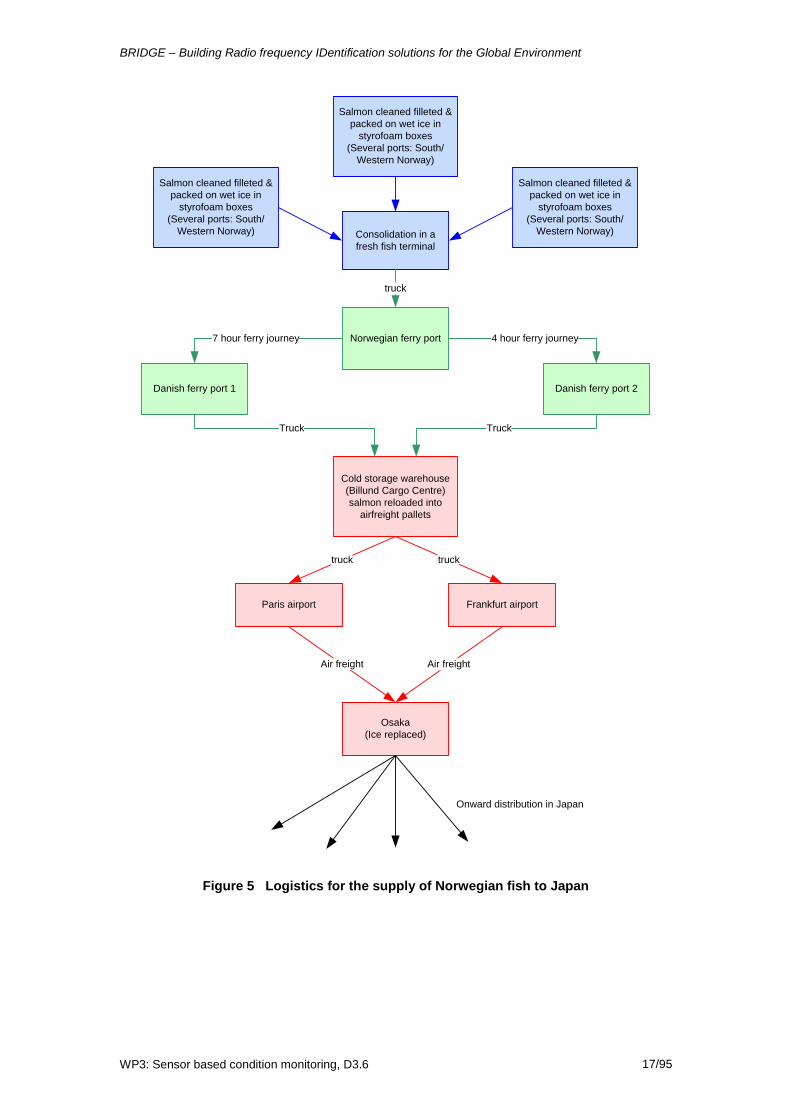
2.3.1 Continuous condition monitoring example In an operation such as industrial-scale fishing, when fish has been caught it is graded by size, washed, chilled and weighed into individual batches which could be in excess of 300kg. In addition to this, basic information, typically including the species, date and time of the catch, fishing location, batch weight and seabed temperature, would be recorded. Clearly, temperature control is essential and is an effective way of slowing bacterial growth, maintaining quality and minimising spoilage. Conversely, high temperatures will cause an increase in the rate of bacterial growth, enzyme activity and also other chemical reactions. To overcome these time-related problems, reliable temperature management is essential to guarantee that the product arrives at its final destination in the best possible condition. Discrete monitoring of the temperature at set time-intervals or process gates may fail to reveal critical breaches in the environmental constraints. To illustrate the challenge, the logistics for the supply of salmon from Norway to Japan [Petersen, 2004] are shown in Figure 5. Fresh salmon that has been filleted and packed on wet ice from several Norwegian ports is consolidated at a fresh fish terminal and then transported by road to a port bound for Denmark. There are two ferry routes that are used and which take different time durations. Once off the ferry,

BRIDGE – Building Radio frequency IDentification solutions for the Global Environment
WP3: Sensor based condition monitoring, D3.6 16/95
the journey continues again by road to a cargo centre, which is affiliated to the various airlines, in Billund. At the Billund cargo centre, the salmon is repacked onto airfreight containers all within an unbroken cold storage chain. From Billund, the fish is transported by road again to either Paris or Frankfurt and flown to Osaka. Once in Osaka, the ice used in the packing is replaced before onward distribution to the final destinations. As can be expected, in this example, there are a number of separate temperature controlled environments that the salmon moved in and out of. Apart from that, there are a number of different parties that have responsibility for ensuring that the cold chain is not broken. In a scenario such as this, there will be a number of statutory checks and controls that have to be performed at each stage of the chain. However, these will not be at item or case level and will be heavily reliant on strict adherence to the handling procedures. To illustrate the different temperature information sources that might be expected in a supply chain, Figure 6 shows a cold supply chain, similar to the above example, from a supplier, through a cold storage facility to an onwards distribution network. In each of these fixed-facility locations, continuous ambient temperature logging is expected that is independent of the chilling plant control. Between each of the fixed locations there would be handling on and off vehicles, containers and aircraft, etc; and these different modes of transport will have yet different devices for monitoring temperature. Again, these temperature monitoring devices are designed for the specific mode of transport and normally rely on manual checks by the receiving party at the destination. As with most supply chains, there are well-established procedures and basic technologies to ensure that products are maintained in optimum condition. There are, however, inevitable failures of systems and processes that can be due to a number of factors:
• Breaks in the cold chain (goods transferred to an uncontrolled environment for a period of time)
• Items stored or transported in an incorrect area or environment (e.g. frozen items in a cool rather than refrigerated area resulting in a freeze-thaw-freeze cycle)
• Inadequate refrigeration on a vehicle for the climate (e.g. unexpected heat wave, significant traffic delays, etc)
• Adjacent packing of ambient or non-cooled products with chilled or frozen products
• Items placed in an airline container, ULD (unit load device) and left on the tarmac in full sunshine for an extended duration
• Human error (or even attempts to mask problems that have occurred and might be undetected)
BRIDGE – Building Radio frequency IDentification solutions for the Global Environment
WP3: Sensor based condition monitoring, D3.6 17/95
Salmon cleaned filleted & packed on wet ice in
styrofoam boxes(Several ports: South/
Western Norway) Consolidation in a fresh fish terminal
Norwegian ferry port
truck
Danish ferry port 1
7 hour ferry journey
Danish ferry port 2
4 hour ferry journey
Cold storage warehouse(Billund Cargo Centre) salmon reloaded into
airfreight pallets
truck truck
Paris airport Frankfurt airport
Osaka(Ice replaced)
Air freightAir freight
Onward distribution in Japan
Salmon cleaned filleted & packed on wet ice in
styrofoam boxes(Several ports: South/
Western Norway)
Salmon cleaned filleted & packed on wet ice in
styrofoam boxes(Several ports: South/
Western Norway)
Truck Truck
Figure 5 Logistics for the supply of Norwegian fish to Japan

BRIDGE – Building Radio frequency IDentification solutions for the Global Environment
WP3: Sensor based condition monitoring, D3.6 18/95
Supplier’s facility temperature Cold storage facility
temperatureVehicle temperature
check
Onward supply chain temperature log
RFID read events
Temperature threshold
Supplier Transport Cold storage facility Transport Onward
distribution
Sensor enabled RFID tag measurements0
1
2
3
4
5
6
7
Time
Tem
p
Figure 6 Sources of temperature data along a cold supply chain
Sensor-enabled RFID is a means of maintaining a complete independent temperature check across the supply chain down to item level. This is illustrated in Figure 6 by the dotted line and blue data samples. It can be noted that the data measured by the sensor-enabled RFID tag does not track the ambient temperatures recorded at the locations. Note also, that in the first transport section of the journey, a number of excursions above the pre-defined temperature threshold have been detected. With current temperature management systems there will be a number of disparate sources of data available; these are likely to be for local use with acceptance/rejection when goods are transferred to and from various locations. Using sensor-enabled RFID (with RFID readers installed at strategic points throughout the supply chain and an underlying EPC network architecture), then either temperature data can be queried across the whole chain or alerts triggered to highlight any potential problems. In either case an accurate time record can be derived, to within the accuracy of the tag's real-time clock, as to when an exception occurred. The purpose and business value of queries about the temperature will depend on the party concerned. For example:
• A supplier might want to be reassured that his goods will arrive in perfect condition.
• A logistics company could ensure that transport conditions are optimal for the items being transported and possibly minimise the energy used to chill the vehicle compartment.
• An end customer (distributor) would have an increased level of confidence that the items received have been transported in the correct conditions.
By contrast, alerts made on the temperature data could: • Trigger the supplier to prepare a replacement shipment
• Enable an end customer to source alternative stock from another source.
An additional benefit of optimised stock control can be derived from sensor-enabled RFID data. This will be discussed in Section 5.

BRIDGE – Building Radio frequency IDentification solutions for the Global Environment
WP3: Sensor based condition monitoring, D3.6 19/95
2.3.2 Discrete condition monitoring example The following use case illustrates an example of discrete condition monitoring in a supply chain. The example is illustrated in Figure 7 and shows the supply chain for the shipment of delicate equipment from the manufacturer in the Far East through to the final location in the Republic of Ireland. Only details of the supply chain from a European distribution centre to a single end country could be obtained but extrapolation to cover the supply chain to the manufacturer’s complete global customer base, and the associated problems, can easily be envisaged. The main challenge when shipping these units is to ensure that they are transported upright throughout the whole journey. If the unit is tilted then they are rendered unusable and require a service engineer to be flown from the Far East to carry out remedial work and checks, etc. Failing that, the units will have to be returned to the manufacturer. The end customer for the units has outsourced the local supply, installation, commissioning and ongoing maintenance to a UK based supplier. The supplier receives the units from the manufacturer’s logistics company at a large DC in Leicestershire (UK). Here they will be offloaded, stored and then transferred to a shipper who takes receipt of the items in Manchester and will route them by road and ferry to a warehouse in Belfast. When installation at the customer’s site is required, a unit will be initially transferred to another smaller site in Dublin before the final move to the customer’s site. Despite the application of single-use passive tilt sensors to the loads, checks were not always made en route to see if individual units had been tilted. In some cases, it was only at the time of installation that the engineers were aware of an earlier problem. Given the high cost and inconvenience caused by a unit that had been tilted, a decision was taken to re-route the units (shown as red arrows in the figure) directly to Dublin and then use road freight to Belfast until required. In this case, single use (non-RFID) indicators were used but have the following limitations:
• They cannot provide absolute values such as the maximum amount of tilt the unit was exposed to or how often the limit was exceed etc.
• They cannot provide any form of time-stamping so there is no possibility of knowing when the limit was exceeded or inferring who was responsible for the mishandling
• Visual inspection is required and all personnel handling the item need to be made aware of the requirement to keep the products upright.
The above limitations could be overcome by using sensor-enabled RFID tags and readers at strategic points in the supply chain. In fact, these devices would be reusable (up to the life of the battery) and, as a minimum, give a timestamp when limits were exceeded. Sensor-enabled RFID would permit the following alerts and actions to be triggered, at or in near real time, based on sensor information:
• Alert to the manufacturer, to schedule an engineer for corrective action
• Alert to inform people handling the unit of its condition before they start to move it & redirect if necessary due to a problem
• Alert to inform the end user that item will not be ready for immediate use

BRIDGE – Building Radio frequency IDentification solutions for the Global Environment
WP3: Sensor based condition monitoring, D3.6 20/95
Transferred to a different vehicle
Transferred to a different vehicle
Original supply route
Units moved to Belfast for temporary storage
Manufacturer(Far East)
Slovakia/Czech Republic via
mainland European port?
LeicestershireDC
Manchester
Belfast warehouse
Dublin warehouse
Destination
Destination
Destination
Destination
Receipt of units from manufacturers distribution chain
Alternative route direct to Dublin
using 3PL
Receipt of units from manufacturers distribution chain
Figure 7 Tilt sensitive logistics from Far East to Ireland
BRIDGE – Building Radio frequency IDentification solutions for the Global Environment
WP3: Sensor based condition monitoring, D3.6 21/95
2.4 Physical and Virtual integration The integration of RFID and sensors in typical sensor-enabled RFID technologies can be achieved using two separate methodologies as shown below:
1) Physical integration: The sensor(s) is connected physically with the RFID tag, and sensor data is read by the RFID reader.
2) Virtual integration: The sensor(s) data is collected independently of the RFID tag, and the integration process is done virtually in the network.
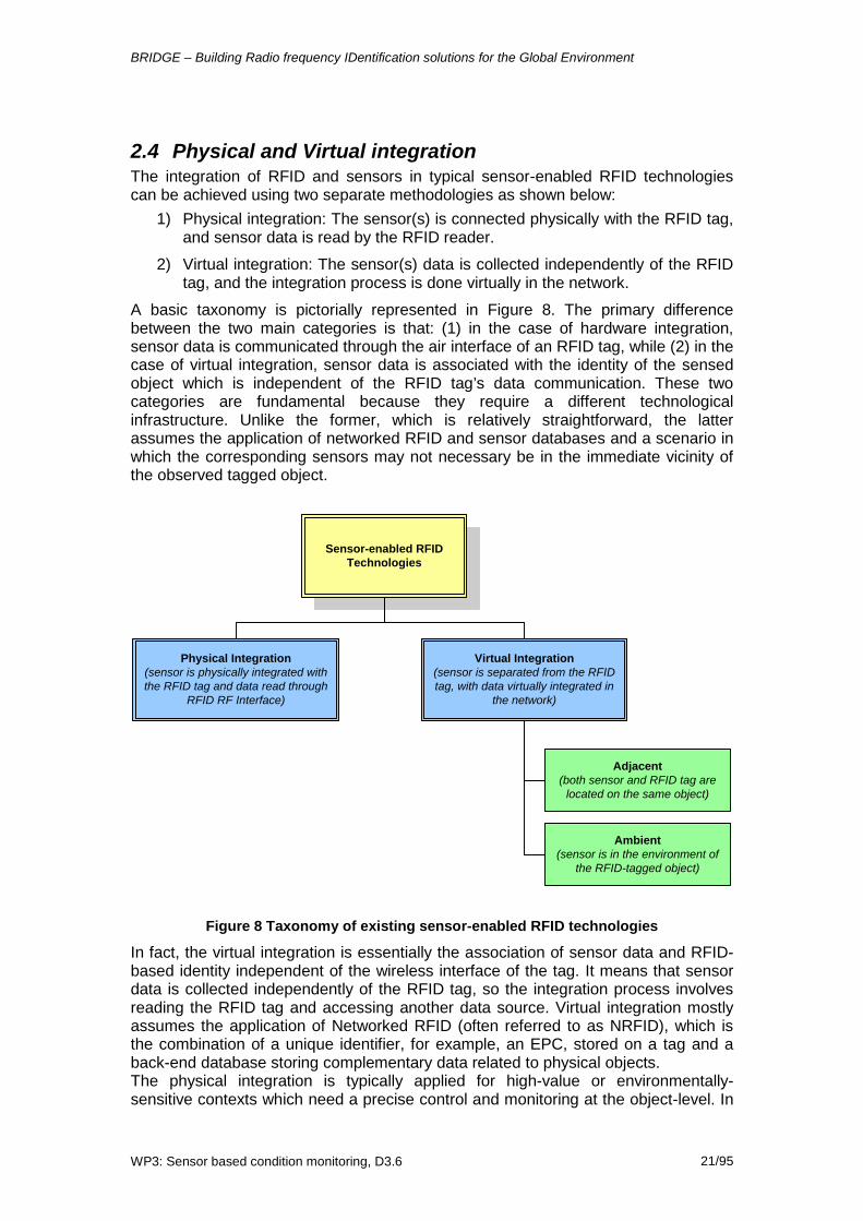
A basic taxonomy is pictorially represented in Figure 8. The primary difference between the two main categories is that: (1) in the case of hardware integration, sensor data is communicated through the air interface of an RFID tag, while (2) in the case of virtual integration, sensor data is associated with the identity of the sensed object which is independent of the RFID tag’s data communication. These two categories are fundamental because they require a different technological infrastructure. Unlike the former, which is relatively straightforward, the latter assumes the application of networked RFID and sensor databases and a scenario in which the corresponding sensors may not necessary be in the immediate vicinity of the observed tagged object.
Sensor-enabled RFIDTechnologies
Physical Integration(sensor is physically integrated withthe RFID tag and data read through
RFID RF Interface)
Virtual Integration(sensor is separated from the RFIDtag, with data virtually integrated in
the network)
Adjacent(both sensor and RFID tag are
located on the same object)
Ambient(sensor is in the environment of
the RFID-tagged object)
Figure 8 Taxonomy of existing sensor-enabled RFID technologies
In fact, the virtual integration is essentially the association of sensor data and RFID-based identity independent of the wireless interface of the tag. It means that sensor data is collected independently of the RFID tag, so the integration process involves reading the RFID tag and accessing another data source. Virtual integration mostly assumes the application of Networked RFID (often referred to as NRFID), which is the combination of a unique identifier, for example, an EPC, stored on a tag and a back-end database storing complementary data related to physical objects. The physical integration is typically applied for high-value or environmentally-sensitive contexts which need a precise control and monitoring at the object-level. In

BRIDGE – Building Radio frequency IDentification solutions for the Global Environment
WP3: Sensor based condition monitoring, D3.6 22/95
contrast, the virtual integration is more suitable for objects where its attributes can be monitored externally by means of a single sensor commonly shared among multiple objects. The latter hence poses a more cost effective solution when compared with the former in the context of low-value goods and business applications with high monitoring tolerance.
2.5 Confidence level of sensor-enabled information The confidence level of the sensor-enabled RFID technologies is dependent on a number of parameters. The factors that will have an impact on the uncertainty are likely to be application dependent, and include the various factors listed in Table 2.
Table 2 Physical factors affecting measurement uncertainty
Accuracy Accuracy of the measurement relative to a reference Precision The degree of refinement in a measurement, calculation, or
specification, especially as represented by the number of digits or decimal places given. Can also be considered as the degree of reproducibility of a measurement.
Calibration The measure of error when compared with reference to an absolute value
Drift A variation of accuracy over time Hysteresis A ‘memory’ effect resulting in a delay before a reliable
measurement is obtained Linearity Constant relationship between input parameter and output value Range Measurement constraint between an upper and lower bound Resolution Related to precision Sensitivity Ability to detect small values and small changes in value Sampling rate
A sampling period is the measure of the time interval between samples. The sampling rate is the reciprocal of this, typically expressed as the number of samples per unit time (e.g. number of samples per second)
Stability Influence on accuracy and precision relative to time Apart from the calibration and individual characteristics of the physical reader and tags, the largest source of uncertainty is mainly due to where the sensors tags are located in relation to the object being monitored. This is especially true when taking into consideration the micro-climate that exists among the items in an enclosed setup (such as a warehouse, container, truck, etc). To illustrate the case, Figure 9 depicts the three commonly used locations for the placement of sensors in an enclosed environment (e.g. temperature sensors within a lorry environment). For ease of explanation, the temperatures recorded at these locations are labelled as: te (environment temperature), tr (RTI temperature) and tc (product core temperature).

BRIDGE – Building Radio frequency IDentification solutions for the Global Environment
WP3: Sensor based condition monitoring, D3.6 23/95
te
trtc
Figure 9 Confidence levels for the three different sensing locations
The measurement te, also known as ambient temperature, reflects the temperature of the environment. Such ambient measurement is mandatory and widely applied across the industry; but the trade-off of such implementation is that its readings do not always reflect the actual temperature of the product itself, tc. To measure the actual core temperature tr of the product, the best practice is to physically place the sensors within or near to the product itself. Such measurements are highly accurate but the cost of implementation can easily escalate with the number of individual loaded items, and these implementations could also sometimes be impractical. As a compromise between cost and accuracy, the measurement tr are recorded instead at the RTI (Returnable Transport Item) level. Such measurements typically possess less uncertainty and are relatively low cost. As a rule of thumb, the confidence level at each placement location of the sensor, ordered in decreasing uncertainty, can be summarised as follows: ( 1 ) Confidence ( tc ) > Confidence ( tr ) > Confidence ( te )
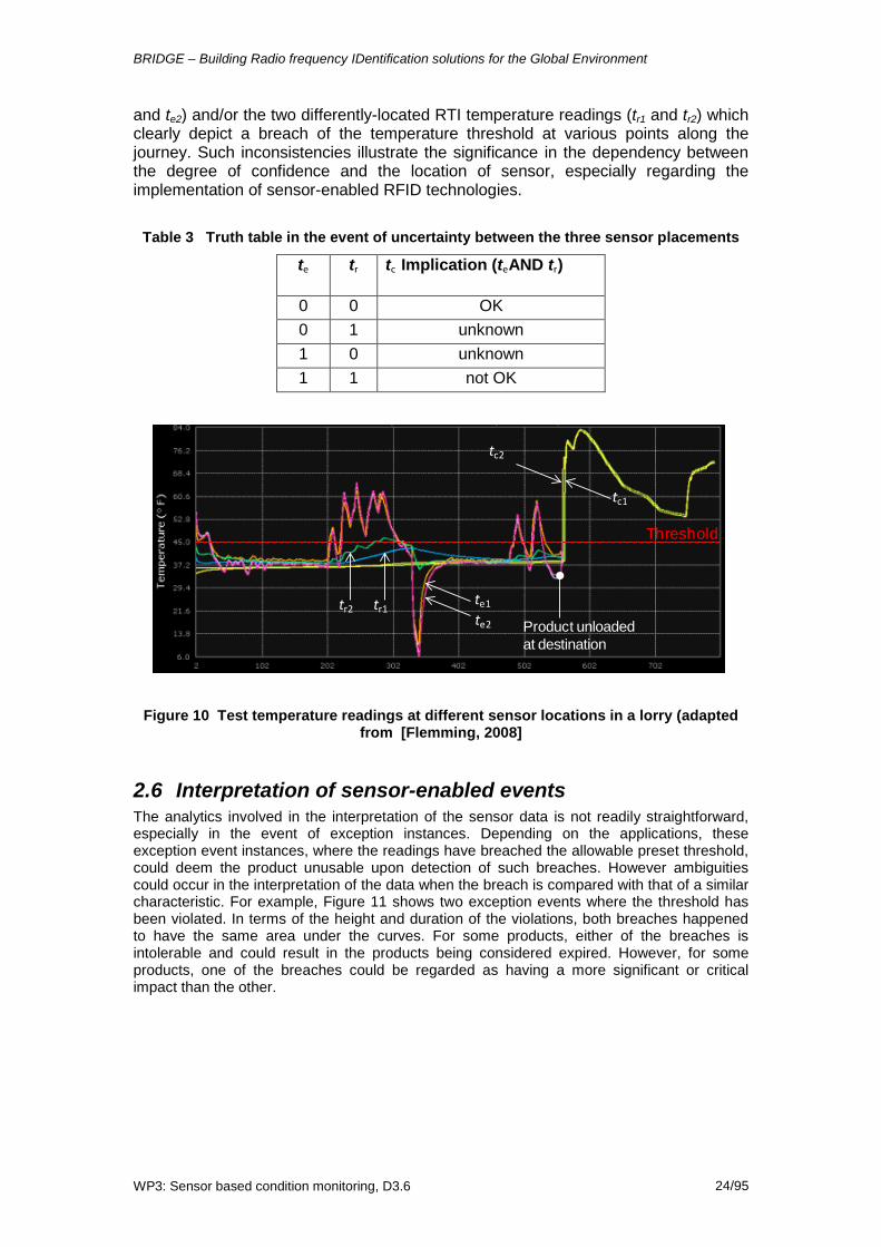
To understand the implication of sensor placement on temperature uncertainties, one can consider a scenario where the measurement of te, and tr are both implemented and monitored in order to infer the actual core temperature of the product itself. Without the presence of the core temperature reading, there is large uncertainty in the condition of the product, especially in the event of exception instances where the product has exceeded its allowable temperature threshold (which hence deemed its products unusable). Table 3 summarizes such ambiguity instances where the measurement of te, and tr are used to infer the condition status of the core product. As can be seen from the table, in the event where there are no exception events (i.e. te= 0 and tr= 0), we can safely infer that the condition of the core product is “OK”; and in the event where exception events are registered in both the te, and tr measurements (i.e. te= 1 and tr= 1), we can infer that the condition of the core product is likely to be “not OK”. However if either of the te, or tr readings record conflicting measurements, the condition status of the core product becomes less certain. To translate that to a real-life example, Figure 10 illustrates the temperature readings recorded at the different sensor locations of a refrigerated lorry carrying loads of perishable goods. In the trial experiment [Flemming, 2008], the refrigerated door of the lorry has been opened and closed to unload some of the goods, at various points of the transportation journey, until the arrival of our goods at their destination. As illustrated in the figure, the core temperature readings (tc1 and tc2) taken at two different locations within the item show that the temperature condition of the product is maintained throughout its entire journey. This is, however, in contradiction with the two differently-located environment temperature readings (te1
BRIDGE – Building Radio frequency IDentification solutions for the Global Environment
WP3: Sensor based condition monitoring, D3.6 24/95
and te2) and/or the two differently-located RTI temperature readings (tr1 and tr2) which clearly depict a breach of the temperature threshold at various points along the journey. Such inconsistencies illustrate the significance in the dependency between the degree of confidence and the location of sensor, especially regarding the implementation of sensor-enabled RFID technologies.
Table 3 Truth table in the event of uncertainty between the three sensor placements
te tr tc Implication (teAND tr)
0 0 OK 0 1 unknown 1 0 unknown 1 1 not OK
tr2te1
te2
tc1
tr1
tc2
Threshold
Product unloaded at destination
Figure 10 Test temperature readings at different sensor locations in a lorry (adapted from [Flemming, 2008]
2.6 Interpretation of sensor-enabled events The analytics involved in the interpretation of the sensor data is not readily straightforward, especially in the event of exception instances. Depending on the applications, these exception event instances, where the readings have breached the allowable preset threshold, could deem the product unusable upon detection of such breaches. However ambiguities could occur in the interpretation of the data when the breach is compared with that of a similar characteristic. For example, Figure 11 shows two exception events where the threshold has been violated. In terms of the height and duration of the violations, both breaches happened to have the same area under the curves. For some products, either of the breaches is intolerable and could result in the products being considered expired. However, for some products, one of the breaches could be regarded as having a more significant or critical impact than the other.

BRIDGE – Building Radio frequency IDentification solutions for the Global Environment
WP3: Sensor based condition monitoring, D3.6 25/95
Same area under curve
Threshold Threshold
Figure 11 Ambiguity example in the interpretation of exception events.
Apart from similar ambiguity characteristics, the way the sensor data has breached the threshold value could play an important role in the interpretation of the data as well. Figure 12 summarises the three typical dimensions commonly employed in the interpretation of exception events: (1) how many times have the exception events occurred, (2) how high/severe are the exception events, and (3) how long do the exception events last?
(1) How many?
(2) How high?
(3) How long?
Figure 12 Three typical dimensions in the interpretation of exception events
As can be seen from the figure, there are a number of ways that the data might exceed pre-determined thresholds. To illustrate the point, let’s examine, in details, the scenario pertaining to each dimension of the event’s interpretation. Figure 13 depicts an instance of the “how many” scenario. As shown in the figure, the exception events in both graphs occur over similar time duration, but the number of times the violations have been breached differs considerably. For products that are sensitive to the frequency of the breach, the lower graph could thus still result in the product as usable as that corresponding to the upper graph.

BRIDGE – Building Radio frequency IDentification solutions for the Global Environment
WP3: Sensor based condition monitoring, D3.6 26/95
0
5
10
15
20
25
0 10 20 30 40 50
0
5
10
15
20
25
0 10 20 30 40 50
Figure 13 “How many” ambiguity scenario
Figure 14 depicts an instance of the “how high” scenario. As seen in the figure, there is a single exception measurement sample that exceeds the threshold by a considerable amount than the other. For some products, these single exception events are trivial and do not cause any significant impact to the condition of the products. However for some products which are sensitive to the height of the breach, the lower graph could deem the product more usable than for the upper graph.

BRIDGE – Building Radio frequency IDentification solutions for the Global Environment
WP3: Sensor based condition monitoring, D3.6 27/95
0
5
10
15
20
25
0 10 20 30 40 50
0
5
10
15
20
25
0 10 20 30 40 50
Figure 14 “How high” ambiguity scenario
Figure 15 depicts an instance of the “how long” scenario. As seen in the figure, the time duration of the exception events differ from one another despite the fact that their frequencies of occurrences are rather similar. For some products which are sensitive to the duration of the breach, the graph at the bottom could be rather tolerable when contrasted with that at the top.

BRIDGE – Building Radio frequency IDentification solutions for the Global Environment
WP3: Sensor based condition monitoring, D3.6 28/95
0
5
10
15
20
25
0 10 20 30 40 50
0
5
10
15
20
25
0 10 20 30 40 50
Figure 15 “How long” ambiguity scenario
In summary, the interpretation of the exception data with regards to its event characteristics and the way the events have occurred is not simple. Depending on the applications, some dimensions of interpretation would be considered more sensitive than the other and would have more significant impact to the condition of the products. The rationale for these dimensions to take higher precedence very much depends on the behavioural properties of the condition of the product; and these will be further elaborated in Section 4.

BRIDGE – Building Radio frequency IDentification solutions for the Global Environment
WP3: Sensor based condition monitoring, D3.6 29/95
3 Supply chain sensor support: Integration of OGC Sensor Web Enablement and EPC network architectures
This section discusses the addition of sensor support to the Supply Chain data gathering services by means of integrating the EPC Network and the OGC Sensor Web Enablement architectures. The objective of this task is to show an alternative integration strategy in which the existing RFID/EPC Network standards are not extended to support new functionalities (i.e. sensor data), but they are linked at an application software layer with other well established standards that implement the required functionality. The EPC Network and the OGC Sensor Web Enablement architectures are chosen due to their leading position in supporting two different technologies: Networked RFID and Web-based sensor systems. The section starts by reviewing the main features of these two architectures and identifying potential synergies. In the second part of the section, a fresh meat traceability case study is used to show step-by-step how the two architectures could be linked and which challenges this strategy would face. Finally, the section proposes a few architectural additions in order to support a flexible set of sensor dispositions, namely ambient sensors, sensors in reusable assets (e.g. RTIs) and multiple sensors per product.
3.1 Background
3.1.1 EPC Network The EPC Network architectural framework is a set of standards for defining, discovering, recording and retrieving unique IDs (EPCs) and related information. The EPC Network currently focuses on observations of uniquely identified objects and the associations between objects, locations, business transactions and business context throughout supply chain processes.
Clients of the EPC Network are able to access event information obtained from RFID systems by querying the EPC Information Services (EPCIS) [EPCIS] interfaces. RFID tag reads are filtered, enriched with business context and stored in on-line repositories, as well as being pushed to clients that have subscribed to queries that match the events. Application Level Events (ALE) provides a standard interface for clients to specify filtering criteria. ALE v1.1 [ALE] also provides methods for reading and writing to tags. The Reader Management standard and recently ratified Discovery, Configuration and Initialisation standard allow for configuration and monitoring of readers. A management application can be used to monitor the health of readers and reader networks. Two systems can be used to obtain the addresses of relevant repositories: The Object Name Service (ONS) [ONS] returns addresses of authoritative information for a particular EPC class; typically it returns the address of the manufacturer's EPC Information Service (EPCIS) repository. Discovery Services provide authenticated authorized clients with addresses of information resources provided by multiple organisations that claim to hold information for an individual EPC and allow multiple organizations to register such assertions and create protected links to their information resources – i.e. other sources of information can be found in addition to information provided by the manufacturer of the product.
3.1.2 OGC Sensor Web Enablement (SWE) OGC SWE [OGCSWE] is a set of standards defined on top of general geospatial standards by the Open Geospatial Consortium. The aim of the SWE is to define architectures and models for defining, discovering, configuring and retrieving sensors and sensor data, in the framework of distributed Web systems. This set of standards provides models to describe sensor data (SensorML [SensorML] and TML [TML, 2007]. The standards also describe how to transform this data into higher-level meaningful information (Observations and Measurements [O&M]). The role of the Sensor

BRIDGE – Building Radio frequency IDentification solutions for the Global Environment
WP3: Sensor based condition monitoring, D3.6 30/95
Observation Service (SOS) [SOS] is to receive observation queries from the clients and respond according to the sensors and sensor systems that are under its management. SOS also gives clients access to the information about the sensors themselves and their capabilities (metadata described in SensorML or TML). Due to the complexity that an observation query might involve, a planning service (Sensor Planning Service – SPS [SPS]) is also defined, through which clients can request query feasibility prior to querying for the data itself. A Sensor Alert Service (SAS) [SAS] provides ways of alerting clients about particular sensor conditions, either by synchronous or asynchronous means (the latter using the Web Notification Service – WNS [WNS]. Finally, a generic catalogue (repository) service (CS) is defined by OGC that can be used within the SWE used in its CS-W extension for discovering data [CS].The OGC SWE standards are described in more detailed in section 6.3
3.2 Initial side-by-side comparison
3.2.1 Similarities between architectures: Table 4 Similarities between EPC Network and OGC SWE and involved standards
EPC Network OGC SWE
Repository of observations & data EPCIS SOS
Discovery Services Discovery Services CS-W Catalogue
Filtering ALE, Reader Protocol SOS (SAS & SPS)
Single point-of-entry queries EPCIS query interfaces SOS (SAS & SPS)
Alerting service EPCIS/ALE standing queries SAS & WNS
3.2.2 Differences • OGC SWE data sources (either sensors or sensor systems) need to register to the
capture service before data can be pulled. Registering aids the query / discovery of sensor by attributes in which the service is based.
• OGC SWE doesn't require global IDs, and thus does not offer any service similar to ONS. To access data of a particular sensor by ID, a query with the data of interest has to precede the data query itself, which returns a locally unique ID.
o There is no specification on how to construct these IDs, and they are supposed to be auto-generated by the system. However, nothing stops developers from tweaking the response of the system with these IDs, so in practice, any ID could be used, as long as is, at least, locally unique.
• The EPC Network provides mechanisms for ALE reports or results of EPCIS queries to be directed to a URI address specified by the user that registered the standing query. OGC SWE supports WNS inside the SAS standard.
• Although more a design decision than a difference, OGC SWE alerts are not originated in the data repository. Instead, there is a separate service independent from the repository to which alerts are sent directly from the data sources. This service, called SAS, just forwards the alerts to any registered client.
• OGC SWE has no concept of base station(BS) or reader management, and treats sensors, sensor nodes and sensor systems as equivalent data sources that have to fulfil the requirements of the standards (registrations, answer to queries, data delivery, etc).

BRIDGE – Building Radio frequency IDentification solutions for the Global Environment
WP3: Sensor based condition monitoring, D3.6 31/95
• There is no planning element in the EPC Network, partly due to the simpler requirements of data capturing and greater homogeneity / limited complexity of the EPCIS event data model1
• The EPC Network does not specify the delivery of data through other mechanisms rather than interface responses, although multiple message transport bindings are permitted
.
2
3.3 Identified synergies and recommendations
. OGC SWE supports multiple ways of data delivery though WNS (although WNS is particularly suitable for asynchronous communication of alerts and planning responses)
• Use SensorML for describing sensor metadata and sensor data model.
• Investigate if TML provides any additional concept needed
• Use SOS/SPS methodologies for querying and filtering sensor data and metadata. This implies:
o Adopt the Observation and Measurements (O&M) [O&M] standards since SOS works mostly with these and not directly with SensorML (which is used only for describing metadata)
o Require that sensor nodes / Base Stations discover / register to the local SOS service
o It is inappropriate to use EPCIS 1.0 to store sensor events and metadata because the current EPCIS 1.0 query language is not sufficiently expressive or flexible.
• The sensor IDs used by SOS don't have a defined format. URIs for the sensorIDs could be used, which are transferred at registration time.
o From the point of view of SOS, it is not important if a registration is done by a sensor, a sensor node, a Base Station (BS) or another system. In this sense, a BS could register the sensor nodes or the BS could be registered as a sensor system providing all the sensor capabilities of their sensor nodes.
o SOS could be queried either by EPC or sensor data / metadata.
• Orchestration of separate repositories and discovery services o EPCIS would be used for supply chain related events, and if sensor data is
required, SOS should be queried.
o SOS could be queried first if it is necessary to obtain object IDs / data that have certain capabilities. Then EPCs obtained from SOS could be used to query EPCIS for relevant supply chain transactions (i.e. which objects were in contact with a particular EPC)
o SOS addresses could be added to ONS or Discovery Services as additional service types, alongside EPCIS
o Separate discovery services for sensor data and EPC Network data are possible but probably not desirable. An integrated discovery service could support queries that involve both EPCs/transactions and sensor information (e.g. obtain addresses of nodes which participated in a particular transaction and which support certain sensor capabilities)
Although both the OGC SWE and the EPC Network include their own discovery services (CS-W and EPC Network Discovery respectively),
1 EPCIS can return a 'QueryTooComplex' or 'QueryTooLarge' exception, which is probably the
nearest equivalent. 2 EPCIS supports a general purpose notification URI to allow results of standing query subscriptions
to be delivered via any mechanism indicated by that URI.

BRIDGE – Building Radio frequency IDentification solutions for the Global Environment
WP3: Sensor based condition monitoring, D3.6 32/95
it would probably be easier to extend the EPC Network Discovery Services to support sensor metadata as defined in OGC SWE. EPC Network Discovery requirements include some very specific requirements about protecting confidentiality of information that could otherwise reveal volumes and flows of goods, so it would probably be the more complex problem to solve.
o An interface to ease the process of querying multiple repositories and services could be developed, such as an enhancement to the Event Gathering Layer developed in BRIDGE WP3, Task 3.2
• SOS has no direct way of updating dynamic metadata. It would probably be good to define an additional optional operation called UpdateSensor in order to update sensor dynamic data, or extend the current RegisterSensor to allow sensor metadata updates. Metadata is information about the sensor (currently encoded in SensorML in the OGC SWE) that is not the data it produces. Dynamic metadata is metadata that can be configured in the sensor, such as reported ranges, reporting format, and so on.
3.4 Case Study: Fresh meat traceability
Breeding Slaughtering Dissection Packaging / Selling
In trucks On pallets or other reusable
assets
On pallets or other reusable
assets
Into trays
F1
F2
F3
F4
S1
S2
S3
P1
P2
FP D1
D2
R1
R2
R3
C1
C2
C3
C4
CattleFarm
Slaughter house
Processing Further processing
Distribution center
Retail End consumer
Generic Process
Supply Chain Scenario
Shipping Receiving
Transport to further
processing
Transport to Slaughterhouse
Figure 16 Fresh meat use case

BRIDGE – Building Radio frequency IDentification solutions for the Global Environment
WP3: Sensor based condition monitoring, D3.6 33/95
3.4.1 Background The objective of this scenario is to judge if the proposed merging of the OGC SWE framework and the EPC Network would provide sufficient functionality to enable real-life condition monitoring and tracking. This scenario assumes that:
• For each item to be monitored, RFID data is read and stored in a local EPC network instance (EPCIS), and sensor data is read and stored in a SOS instance. This means that, as a principle, we assume that the sensor readings can be unequivocally and automatically matched with a specific item3
o For RFID only, at least once at each supply chain step (preferably upon arrival) and once every time aggregation and decomposition occurs. Aggregation and decomposition is recorded and stored in the EPCIS of the entity where the event is generated.
. We further assume that the data capture happens in the following way:
o For sensor information, at least once at the arrival at each supply chain step, and then periodically according to any real-time needs for the condition to be monitored.
• Either a catalogue service exists at each supply chain step that points to the SOS and that can be accessed by the sensors/sensor gateway, or a generic gateway at each step is able to read the sensor data without sensor reconfiguration and is configured to contact the SOS of that step (the last being very similar to what RFID readers do).
• Once the address of the SOS is known, the system in place (be it individual sensors or a certain gateway) registers every sensor source. This happens prior to the first data capture at each step.
• Discovery services would be functional and either there are no security and privacy issues involved in the data sharing or they are addressed by the implementation of the discovery services.
As a general statement, these assumptions mean that for each relevant item in the supply chain, mechanisms exist that allow its ID and sensor data to be read and stored in EPC Network and OGC SWE instances respectively, with the desired periodicity and granularity, and that discovery and catalogue services exist that allow the access to that data from a given (authorised) client.
3.4.2 Functionality As the functionality of our particular scenario, we will require that:
1. Sensor and ID information is captured and stored in both OGC SWE and EPC network respectively, with appropriate cross-referencing mechanisms
2. This information can be retrieved for historical data analysis
3. An alert is sent to the client if the temperature of the meat, at any stage of the supply chain, exceeds a certain threshold. Note that the time accuracy of this depends on how often the data is read. Periodic updates are assumed.
3.4.2.1 Data Capture Regarding the first functionality point, it is achieved by meeting the previously listed assumptions: at each stage of the supply chain, ID and sensor data are independently captured by each architecture. 3 Another option, such as the use of ambient sensors, will be discussed at the end of the
discussion.

BRIDGE – Building Radio frequency IDentification solutions for the Global Environment
WP3: Sensor based condition monitoring, D3.6 34/95
Regarding the RFID architecture, this section does not discuss in detail how the information flows from tags to Information Services since this is a widely documented elsewhere [EPCglobal]. Typically, the EPC Network architecture for a supply chain is replicated at each step (e.g. Farm, Slaughter house, Distribution centre, etc ) such that each has its own implementations of Readers, ALE [ALE] and EPCIS [EPCIS]. Via interaction with the ONS [ONS] and Discovery Services, supply chain clients can gather all the information distributed in the databases across the whole supply chain (or, at least, the information they have permission to access).
In a similar way, an OGC SWE architecture for a supply chain would be distributed in the same way. This is not a design limitation, but rather an implementation decision based on the notion that the organizations that govern each supply chain step want to have control over the data that is produced in their step of the supply chain. This implementation decision is analogous to that of the EPC Network.
For simplicity, we will ignore the OGC SWE components that are not fundamental for obtaining the functionality that we require. This only includes the SPS, since an alerting service (SAS + WNS) is very desirable for a scenario involving sensor data. However, note that we could proceed without the alerting service and limit our knowledge to an analysis of the historical data when the meat arrives at the retailer.
SOS
BS
Filter
Sensors / sensor systems
SAS
WNS
Client Interface
SOS
BS
Filter
Sensors / sensor systems
Discovery(CS-W)
SAS
WNS
SOS
BS
Filter
Sensors / sensor systems
SAS
WNS
Farmer Slaughter house
Retail. . .
Figure 17 Possible OGC SWE installation for the Supply Chain
Figure 17 depicts a possible installation of the OGC SWE for our Supply Chain scenario. Note that the only non-replicated shared component is the catalogue service, which clients (sensor devices, Base Stations and other clients) use to discover SOS instances in a similar way to how Discovery Services are used in the EPC Network to discover EPCIS instances. Regarding the replication of components by each organisation, it is worth considering sensor values and how they are used to represent the condition of a given item (meat, in our case). It may be reasonable to think that for a sensor value that is associated with meat, the criteria used to raise alarms would be the same across its supply chain, post-slaughter. For example, if it is decided that above +5 °C, a beef product is in danger of being spoiled, this threshold value would apply regardless of at which step of the supply chain the meat is. It is also true, however, that alarm recipients would probably vary, so a single service with a single subscription will not suffice. The design of SAS allows for sensors to advertise their capabilities and clients to define alerts regarding those capabilities. It could be possible, thus, to provide a central alert service to which a sensor belonging to a meat item would advertise

BRIDGE – Building Radio frequency IDentification solutions for the Global Environment
WP3: Sensor based condition monitoring, D3.6 35/95
and to which any client could subscribe independently. This could solve the component replication issue in that it is not necessary for the same sensor to advertise in every supply chain step. However, it would not solve the problem of multiple subscriptions with the same criteria, since there is no mechanism to support the discovery of existing subscriptions. In any case, providing a centralized SAS service would create a similar problem to that of creating a centralized SOS: In the SAS design, sensors publish their data to the service, which effectively becomes a hub through which all the sensor readings, IDs and timestamps pass. This would surely become a confidentiality concern for the various organizations that send the data. We can thus conclude that the replication of SAS+WNS in all the supply chain steps is probably the best solution.
For a sensor to be able to publish data in a SOS repository, it must first register with the repository. The registration could be done by the sensor itself (in which case the sensor/sensor node needs to be able to encode XML messages) or could be done by the BS on behalf of the sensor. The registration will only be used while the item remains within that organization4
We have described so far how both the ID data and the RFID data are stored in distributed databases (EPCIS and SOS) along the supply chain. We now need a mechanism that will match both data streams and that can be queried seamlessly. The SOS returns a RegisterSensor response upon registering a sensor. This response includes an AssignedSensorID, which by default will be randomly chosen by the SOS. We would like, however, to know this ID beforehand or, more specifically, be able to inject a known ID instead of letting the SOS choose one for us. The reason for this is that without a known ID it would be impossible to retrieve information about a specific sensor, a step that is required in order to match EPCNetwork IDs and OGC SWE sensor data. To be able to control the assignment of the sensorID, we could include this information as part of the SensorDescription when registering the sensor, and program the SOS so it will read, assign and return this ID as a response of the registration. This identifier is described as “of type anyURI” by the SOS specification. Section
. Note that the address of the SOS is not known a-priori by the sensor (each SOS from each organisation has a different address). The sensor would thus need to discover the SOS using the Discovery Service. Once that happens and a sensor is registered, data can be published and can be queried or discovered by clients. In case the registration is done by a BS on behalf of one or multiple sensors, the BS could be pre-installed with the address of the SOS. Other combinations are also possible. For example, the BS (active tag reader) could know the address of the SOS and let the sensor nodes learn it when they first communicate. In this case, the sensors would still register to the SOS by themselves but no discovery mechanism would be necessary.
3.4.3 will discuss which type of ID should be injected into the SOS registration.
3.4.2.2 Data Retrieval The methodology that we are proposing here combines two independent architectures. For this reason, a client should either invoke independent procedures to retrieve data from them, or we should provide an orchestration component that takes unified client requests and coordinates the connection with both architectures to provide a unified answer. In any case, the intention of this section is to prove that meaningful condition information unequivocally linked to “legacy” EPC information can be obtained by using the approach presented here.
For similar reasons as explained in the previous section, we will not explain in detail the intricacies of EPC Network data retrieval. We will assume, however, that the goals of accessing additional sensor data from the OGC SWE architecture are the following:
o To be able to obtain condition data for meat (or other perishable goods) associated with a specific EPC and for a particular time period and/or location.
o To be able to issue alarms under particular conditions (e.g. relating to food safety)
4 Interestingly, it seems that there is no operation to cancel a registration. This means that once the data of a sensor has been inserted after registration, it can't be deleted.

BRIDGE – Building Radio frequency IDentification solutions for the Global Environment
WP3: Sensor based condition monitoring, D3.6 36/95
o Once an alarm is raised, to be able to analyse the trace of the offending meat product in order to determine partners potentially responsible for unsafe handling conditions.
o To be able to query historical condition data.
Sensor data is sent to the SOS encoded in Observations as specified by the O&M OGC SWE specification. The O&M specification is very complete and flexible, and includes among other things time stamps and multiple ways of defining locations. In the EPC Network, time-stamped records are captured at the EPCIS layer and include two types of locations, the ReadPointID and the BusinessLocationID. A match between the OGC SWE and EPC network time-stamps might be trivial if understood correctly. Regarding the locations, it is evident that O&M allows much more complex specifications (e.g. geometric areas). It is also evident, however, that it would be possible to use similar location IDs in both architectures in order to ease the integration of both sensor and ID data streams. To this extent, we may thus want to extend the Observations sent by the sensor nodes with custom fields called ReadPointID and BusinessLocationID. This extension would be most suitable for fixed sensors (I.e. ambient sensors) as presented in Section 3.4.3.1.
The SOS supports two types of queries that are of interest to our proposal. The first query is called getObservation and allows a client to request the retrieval of any type of data according to the O&M structure. This includes location and time. The second query is called getObservationById and allows the retrieval of data directly based on sensor IDs. As explained earlier, by being aware of which sensorIDs represent which product (i.e. by controlling their assignation), it would be straightforward to retrieve both ID and condition data based on the product instance identifier (EPC).
Finally, alarms naturally provide the ID of the offending sensor when they are triggered. They also inherently provide the time that the alarm was produced. Additionally, further sensor details can be accessed by querying the SOS with the same sensor ID. It would also be possible to extract the EPC and timestamp of a meat product from an alarm and use that information to query the Discovery Service and relevant EPCIS (or the SOS) to obtain a trace of what happened prior to the alarm being triggered.
3.4.2.3 Alerts The Sensor Alerting Service (SAS) of the OGC SWE specification supports the subscription and triggering of alerts based on sensor data. SAS works independently from SOS, so sensors wishing to participate in alerts also need to subscribe to SAS even if they already subscribed to SOS. One of the advantages of this approach is that the sensor description doesn't need to be the same (e.g. it is possible to register a single alarm for a set of sensors). Unfortunately, for this same reason the SensorID returned from SAS upon registration is unrelated to the SensorID returned by SOS. Let's assume that our interest is to receive alarms from specific items. In this case, we would like to be able to inject the SensorID and so relate it to the product, the same way we registered the sensor with the SOS. For this purpose, the sensor would have to send the ID to the SAS in its advertisement (Advertise operation), so SAS can use the injected ID as the SensorID instead of generating one ID by itself. Unlike the O&M, the SAS specification, which has not been updated since 2006, does not provide a wildcard field that can contain extra information, although the description of SensorID specifies a “Unique ID for every registered sensor, usually set by SAS”. In any case, we could easy extend the XML encoding of an Advertise request to include an extra ID field, and program the logic of the SAS so this ID would be used as the SensorID in the Advertise response. From that moment, all the operations that refer to any alert coming from that sensor will include the injected ID that is related to the relevant product.
Sensors register their capabilities, while subscribers register their interest in specific conditions of those capabilities. SAS offers an interface for clients to discover and subscribe to alerts of registered sensors. Once registered sensors have been discovered, SAS provides a language to allow clients to express filters that specify which sensor data they want to receive. In this way, only the sensor data that passes through the filter will be forwarded to the clients. This sensor data is encoded together with the SensorID and timestamp.
SAS uses XMPP (Extensible Messaging and Presence Protocol) to allow clients to subscribe to a particular stream of sensor data. Subsequent alerts are delivered either by the XMPP

BRIDGE – Building Radio frequency IDentification solutions for the Global Environment
WP3: Sensor based condition monitoring, D3.6 37/95
protocol itself, or by other means using the WNS OGC specification (supporting protocols such as e-mail, HTTP, SMS, or FAX). Once the alerts have been received, clients can extract the information and request further information from other services (e.g. SOS or EPCIS Network) if necessary.
3.4.3 Sensor disposition and ID assignation As mentioned in section 3.4.2, the assumption for the previous argumentation was that any sensor data can be matched unequivocally with a particular item, specifically via the EPC of the product. Technically, this could be achieved either by using a single sensor tag in each product or by combining one sensor tag and one passive tag. In the former case, the Base Station and Reader used for capturing data would be the same for both the EPC Network and the OGC SWE, and in the latter case they would be different. Since the handling of sensor data at any level of the EPC Network is not yet standardized, it is likely that an actual implementation would have to use standard passive RFID tags together with some proprietary sensor tags (e.g. wireless sensor nodes). In this case, it would be necessary to be able to map the ID of the sensors to the ID of the products they are representing. There might be several ways of assuring this mapping, and they might depend on the disposition of the sensors in relation to the product that needs to be monitored. However, it is paramount to devise a system that would be flexible enough to adapt to all the possible disposition scenarios. This section discusses the most relevant of these scenarios and tries to design a cross-reference mechanism that satisfies all of them.
3.4.3.1 Ambient sensors We now consider the use of “ambient” sensors and item-level passive tags. In this approach, the sensors are located in the environment that surrounds the actual meat items, and a middleware layer is used to extrapolate the ambient sensor readings to each item. In this case, the matching of sensor data and identification data is not one-to-one, but one-to-many, as one sensor reading would be assigned to all the items that were located, at the same time, in the area of influence5
The implementation of this latest option bears a certain difficulty and needs the development of a software layer with access to both the EPC Network architecture and the OGC SWE. This software layer could be a more complex version of the orchestration component that was mentioned earlier. For each piece of integrated information requested by the client, a comparison of location should take place from records of the EPCIS and SOS. For example,
of the sensor. Technically, the difficulty of the implementation of this approach resides in how to decide which sensor reading is assigned to which item. It could be argued that the most straightforward way would be to do this by matching locations, either by developing a simple locationID comparison (e.g. Reader 1 is located in Room 2, so all the sensor values from Room 2 are assigned to any item read by Reader 1) or by comparing geographical locations (e.g. Reader 1 is located in coordinates (x,y,z), and the area of influence of Sensor 2 is determined by the polygon W. If (x,y,z) is contained in polygon W, then readings from Reader 1 will be assigned to Sensor 2). Furthermore, we should make an approximation of how long an item has remained within a given area of influence of a sensor. Doing so would involve taking into account that a passive RFID reading point is discrete, and depending on the travelling speed of the item it could have remained in a certain area for a longer or shorter time.
5 We must not confuse Sensor Range and the area of influence of a sensor. A sensor range extends exactly to the area where the sensor can physically capture a particular phenomena (or, at least, the area that has been determined that the sensor can capture the phenomena lie within a particular confidence value). A sensor area of influence is the area represented by a particular sensor, as determined a priori. A sensor area of influence could be equal or smaller than the sensor range. Typically, sensor ranges overlap between adjacent sensors, but sensor areas of influence do not.
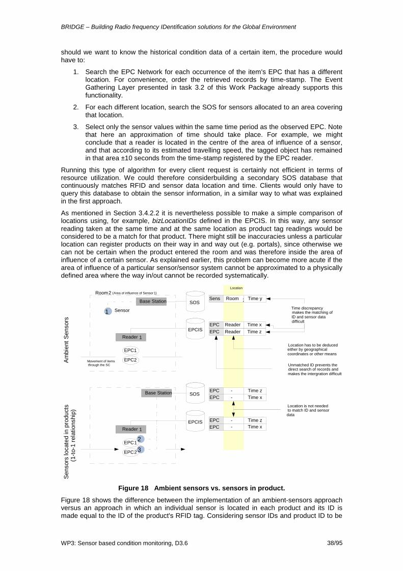
BRIDGE – Building Radio frequency IDentification solutions for the Global Environment
WP3: Sensor based condition monitoring, D3.6 38/95
should we want to know the historical condition data of a certain item, the procedure would have to:
1. Search the EPC Network for each occurrence of the item's EPC that has a different location. For convenience, order the retrieved records by time-stamp. The Event Gathering Layer presented in task 3.2 of this Work Package already supports this functionality.
2. For each different location, search the SOS for sensors allocated to an area covering that location.
3. Select only the sensor values within the same time period as the observed EPC. Note that here an approximation of time should take place. For example, we might conclude that a reader is located in the centre of the area of influence of a sensor, and that according to its estimated travelling speed, the tagged object has remained in that area ±10 seconds from the time-stamp registered by the EPC reader.
Running this type of algorithm for every client request is certainly not efficient in terms of resource utilization. We could therefore considerbuilding a secondary SOS database that continuously matches RFID and sensor data location and time. Clients would only have to query this database to obtain the sensor information, in a similar way to what was explained in the first approach.
As mentioned in Section 3.4.2.2 it is nevertheless possible to make a simple comparison of locations using, for example, bizLocationIDs defined in the EPCIS. In this way, any sensor reading taken at the same time and at the same location as product tag readings would be considered to be a match for that product. There might still be inaccuracies unless a particular location can register products on their way in and way out (e.g. portals), since otherwise we can not be certain when the product entered the room and was therefore inside the area of influence of a certain sensor. As explained earlier, this problem can become more acute if the area of influence of a particular sensor/sensor system cannot be approximated to a physically defined area where the way in/out cannot be recorded systematically.
EPC 1
Reader 1
1 Sensor
Room 2 (Area of influence of Sensor 1)
EPC 2
SOS
EPCISEPC 1Reader 1 Time xEPC 2Reader 1Time z
Sens 1Room 2 Time y
EPC1
Reader 1
EPC2
SOS
EPCIS
EPC 1 - Time z
2
3
Base Station
Base StationEPC 2 - Time x
EPC 1 - Time zEPC 2 - Time x
Location
Location is not needed to match ID and sensor data
Time discrepancy makes the matching of ID and sensor data difficult
Sens
ors
loca
ted
in p
rodu
cts
(1-to
-1 re
latio
nshi
p)A
mbi
ent S
enso
rs
Location has to be deduced either by geographical coordinates or other means
Unmatched ID prevents the direct search of records and makes the intergration difficult
Movement of items through the SC
Figure 18 Ambient sensors vs. sensors in product.
Figure 18 shows the difference between the implementation of an ambient-sensors approach versus an approach in which an individual sensor is located in each product and its ID is made equal to the ID of the product's RFID tag. Considering sensor IDs and product ID to be

BRIDGE – Building Radio frequency IDentification solutions for the Global Environment
WP3: Sensor based condition monitoring, D3.6 39/95
equal is a rather simplistic approach, but enough for the purpose of understanding the implications on the use of ambient sensors or where there is only one sensor per product instance. Other options regarding the number of sensor per product and unequal IDs are discussed in the following sections.
3.4.3.2 Sensors in reusable assets Rather than attaching sensors to each individual product, it also possible to attach them to the reusable assets (i.e. RTIs) that transport those products along the supply chain. Examples of these reusable assets are trays, pallets or even containers. This option may be desirable due to the fact that it reduces cost in the potentially costly sensor devices, both reducing their numbers and making them reusable. We now discuss how this scenario would affect the proposed architecture.
A shared sensor device in a reusable asset carrying several meat products implies that there can not be a one-to-one correspondence between sensor ID and product ID. The question that we should answer is therefore, given a product's EPC, how to find out the ID of the sensor of the reusable asset in which it was stored or transported. Of course, if the reusable asset changes in any way (e.g. aggregation of pallets, change to a new reusable asset) we should also be able to find this out.
Probably the first possibility that comes to mind is to use some kind of aggregation-disaggregation tracking service that records when a product has been put in a reusable asset as well as when is has been removed. The EPC Network already enables this by means of aggregation events within the EPCIS event data model, and the Event Gathering Layer developed in BRIDGE WP3 provides a mechanism for automatically following such changes of aggregation. By using this functionality, we could ultimately know which reusable asset was transporting which product at any point in the supply chain. The problem with this approach is that, for the EPC Network to be able to capture the reusable asset's ID data (and thus record the aggregation events), the reusable asset must have a tag that can be read by the EPC Network readers. Now, to achieve this, we could either use special tags that can be read by both the OGC SWE gateways and the RFID readers (i.e. EPC compatible sensor tag), or we could have a separate device for the sensor data (e.g. sensor node) and RFID data (e.g. passive RFID tag). In the former case, there is no such well-established device. In the latter case, we find the additional problem of how to match the ID or EPC of the passive tag with the sensor device ID so we can associate the sensor reading with the reusable asset and hence with the products transported with it. For example, imagine that the EPC Network has recorded all the aggregation events along the supply chain of trays with the meat products. Therefore we know which product has been in which tray and when. The OGC SWE's SOS has collected sensor data from all the trays, and has assigned to the sensors in those trays some ID, either automatically or by some kind of strategy as explained earlier in Section 3.4.2. We need to be able to match the sensor ID with the tray ID in order to infer the condition of those meat products. In this respect, we find the following possibilities:
1. The company in charge of managing the reusable assets makes sure that the sensor device in the tray knows the EPC of the tag in the tray. A mechanism is set so this EPC is assigned as the ID of the tray’s sensor.
2. The company in charge of managing the reusable assets assigns any ID to the sensor device in the tray, but makes sure that there is a networked and automatic way of matching both IDs. An example could be an EPCIS server discoverable via ONS containing this correspondence between the EPC for each tray provided by the company and the IDs of the sensors that it contains. Ideally the sensor IDs should be globally unique in this situation.
3. The matching is done using location and time of the readings. The problem with this approach is that there must be an unequivocal match of time and place for both the data captured by the OGC SWE gateway and the RFID reader. This assumption might be reasonable for reading one tray at a time, making sure that both RFID antennae only capture data from that tray. However, if multiple trays are read at the same time, it is not possible to distinguish which sensor data came from where in an accurate way.

BRIDGE – Building Radio frequency IDentification solutions for the Global Environment
WP3: Sensor based condition monitoring, D3.6 40/95
3.4.3.3 Multiple sensors
Client
EPC(P)Sensor 1EPC(S1)Sensor 1EPC(S1)
Sensor 2EPC(S2)
SOS
BS
FilterALE
EPCIS
Reader
ALE
EPCIS
Reader
ALE
EPCIS
Reader
ALE
EPCIS
Reader
EPCIS
Product Sensor1 Sensor2
EPC(P) EPC(S1) EPC(S2)
... ... ...
EPC(P) aggregated withEPC(S1) and EPC(S2)
Sensor 1 and Sensor 2registered individuallywith IDs EPC(S1) and
EPC(S2)
Manufacturerlogistics or others
Product / re-usable asset
ONS
Figure 19 Players with several sensor devices per product or reusable asset
When a sensor is registered with the OGC SWE, it does not need to do so as an individual sensor, but it might register a sensor system (e.g. sensor node) which can provide several sensor readings. This registry will have a single sensorID, no matter from how many physical sensor devices the information comes from. This is analogous to the concept of a 'logical reader' at the ALE layer [ALE] of the EPC Network or a 'readPoint' at the EPCIS [EPCIS] layer of the EPC Network.
Reusable assets: Option number 2 in Section3.4.3.2 could provide more flexibility if several sensor devices were to be installed in the same reusable asset (e.g. large containers or pallets). In this case, it is still advisable to use a single reusable asset ID, although several passive tags with the same ID might be distributed around the asset to improve the reading success. However, it might be problematic to assign the same ID to more than one sensor device. Firstly, multiple registrations with the same ID are not supported, and a mechanism should be devised in order to allow only one registration to the SOS. Secondly, information arriving to the SOS with the same sensor ID would be treated as coming from the same device, and stored as such. This could result in problems such as different locations, clock synchronisation and others. Furthermore, any top-down communication to the sensor devices would be rendered unusable unless the same message should be transmitted to all the sensor devices. Obviously, in any case the sensor devices must be identical so the

BRIDGE – Building Radio frequency IDentification solutions for the Global Environment
WP3: Sensor based condition monitoring, D3.6 41/95
registration information is the same. A registration as a single sensor system could also be possible and would allow the sensor devices to be different, but a mechanism at the base station should be put in place to register the system and merge the messages of the various sensor devices in a single report. Option 2 would allow association of any number of sensor device IDs with a single reusable asset ID. Option 2 thus appears as the more flexible and feasible of the alternatives.
Products: We might want to attach several sensor devices to a single product in a similar way to how we attach several sensor devices to a single reusable asset. The discussion and conclusions of this are also similar to what was discussed in Section3.4.3.2. The only difference is that the EPCIS containing the matching table would have to be managed by either the manufacturer who tags the products, or some third party in charge of installing and managing the sensor devices.
Figure 19 depicts the players that would be necessary using option number 2 and several sensors per product or reusable asset.
3.4.3.4 Structure of the matching repository for multiple sensors Figure 19 shows how clients can match the EPCs of the products/reusable assets and sensor devices by querying a repository held by the manufacturer/logistics company (i.e. matching repository). Although that repository could be of any kind, as long as it answers the question of which sensor devices belong to which reusable asset or product, Figure 19 suggests the use of an EPCIS repository. The main reason for this suggestion is that something similar to EPCIS aggregation events could be also utilized to record the association of products/reusable asset IDs with the IDs of the sensor devices attached to them. In this way, standard and existing methods can be used as well for the matching repository and the interfaces that offer its services to clients and repository holders. Furthermore, because ONS supports multiple service types (and Discovery Services are likely to do so), EPCIS can be easily referenced by existing EPC Network services and thus be integrated inside the EPC Network architecture which already exists in the proposed integrated implementation.
An interesting discussion can be held around the semantics of the existing EPCIS aggregation events and the purpose of the repository. EPCIS aggregation events have been initially designed to track physical 'containment' relationships along the supply chain. Although the relationship between e.g. a pallet and the sensors located on it is also a physical relationship, the aggregation is more likely to happen only once at the beginning of the supply chain, and in the case of reusable assets or location, probably remain like that over a period of time throughout many supply chain cycles of many products carried by the reusable asset. Of course, using EPCIS aggregation events would allow one to change this relationship at any point (e.g. a sensor is broken in transport and replaced in some middle-point), which is nevertheless beneficial in terms of flexibility. However, there might be problems of interpretation by application software when all the items inside a reusable asset have been removed (e.g. it receives an EPCIS aggregation event with action field set to 'DELETE' and childEPCs field set to null), since they might think that also the sensors associated with the reusable asset have been removed, even when it is not the case.
Given the difference in semantics, it might be appropriate to define a new sub-type of EPCIS event that is structurally similar to an aggregationEvent but that would encompass our intended meaning; the semantics of this new sub-type of EPCIS event would not be the same as the aggregation event issued when items are added or removed from the reusable asset, so no confusion about removal of sensors could occur. For the sake of clarity, we could call this new event association event instead of aggregation event. For fixed sensors, the parentID could also be a bizLocation (rather than the event simply occurring at a bizLocation), and this case would represent an association between one or more sensors and a location of the type discussed in Section3.4.3.1 For sensors attached to reusable assets, the parentID could be the EPC or ID of the reusable asset, while the childEPCs field could contain a list of the IDs of one or more sensors associated with that asset.
Other fields such as bizStep, disposition, or bizTransactionList would probably not be used in this new type of aggregation type, although they are already optional fields in the EPCIS specification.

BRIDGE – Building Radio frequency IDentification solutions for the Global Environment
WP3: Sensor based condition monitoring, D3.6 42/95
3.5 Summary We have seen how an independent installation of the EPC Network and the OGC SWE allows a client to retrieve supply chain data based both on ID and sensor conditions in an integrated way. The only additional development needed for this approach to work is an orchestration engine able to access both architectures and interpret the retrieved data in terms of both location and time. Very limited or no additional modification of current standards is needed. A cattle meat supply chain was used as an example, providing all the expected functionality of a condition-based supply chain, including the generation of alerts in real-time and the track and trace of meat products based on ID and sensor data. We have also seen the complexity of various implementation approaches to the system, and discussed how sensors can be distributed either in the environment surrounding the monitoring products, in reusable assets where the products are transported or attached to the products themselves. We concluded that the most flexible approach involves an additional networked repository where identities of sensors and products can be cross-referenced, since this allows the use of unlimited sensor devices per product. We note that in principle these associations between sensor IDs and EPCs of physical objects could even be recorded within EPCIS repositories, as an associationEvent, a proposed new subtype of EPCIS event, similar to an aggregationEvent, but with subtly different semantics.

BRIDGE – Building Radio frequency IDentification solutions for the Global Environment
WP3: Sensor based condition monitoring, D3.6 43/95
4 Factors relating to condition of objects In this section, we will focus primarily on two distinct kinds of objects:
1) perishable objects such as foods, beverages, pharmaceuticals and vaccines
2) objects and assemblies that are subject to mechanical wear and vibration
4.1 Condition of perishable objects The deterioration of perishable objects can lead to a decrease in the aesthetic appeal (such as discolourations, blemishes, and unusual smells), as well as a reduction in nutritional value (e.g. due to loss of vitamins) and potentially the production of poisonous toxins, such as those produced by the bacteria Salmonella and Escherichia Coli.
Sometimes the degradation of foods is readily visible as changes of texture or discolouration, such as the blackening of banana skins as the fruit ripens then passes peak ripeness. In other situations, the degradation might not be so readily visible, even though the efficacy of the object has been degraded. (This may be the case for pharmaceuticals and vaccines).
In other cases, thermal cycling and especially freeze-thaw cycles can result in damage to cell structures or phase separations of emulsions [Robinson, 2001].
Sensors [Kress-Rogers, 1993] can be used in two distinct ways:
1) to monitor the environmental conditions before (and during) deterioration
2) to monitor the factors that indicate the extent of progress or rate of degradation (e.g. discolouration, production of heat or specific gases)
For monitoring environmental conditions, key environmental factors include:
Table 5
Factor Sensor type for detection of pre-conditions
gases such as oxygen, carbon dioxide, ethylene
Gas sensors
relative humidity Humidity sensors high temperatures Temperature (maximum exposure) temperature fluctuations Temperature (maximum, minimum, history) low temperatures (chill injury) Temperature (minimum exposure) exposure to light Photodetectors physical handling (e.g. bruising). Shock sensors & vibration sensors
It is important to note that there is not always a straightforward linear relationship between a sensor measurement (such as temperature) and the quality or safety of a product. The relationship is often complex and may need to consider a number of possible reactions (decay mechanisms), as well as the micro-organisms and enzymes that catalyse those reactions - and in turn, how their activity depends on environmental conditions, such as temperature, humidity, acidity, concentrations of gases such as oxygen, etc.
Furthermore, it is not possible to develop a single universal guideline that is applicable to all kinds of perishable objects. Although there are some general principles, it is also important to be aware of the exceptions to the rules. For example, low temperatures extend the shelf life of many foods, by lowering reaction rates - but can result in chill injuries to tomatoes, squashes and bananas. Likewise, ethene gas can be used to promote the ripening of fruit such as bananas but can result in rapid wilting of freshly cut flowers.
Various reports and handbooks on food science [Norman, 1988] and food chemistry [Belitz, 2004] provide tables that describe the modes of deterioration, expected shelf life [Jones,

BRIDGE – Building Radio frequency IDentification solutions for the Global Environment
WP3: Sensor based condition monitoring, D3.6 44/95
1994] and the critical environmental factors that must be considered for each category of perishable or semi-perishable food.
The fact that a particular object is perishable means that over a period of time and exposure to particular conditions in its immediate environment, its quality may degrade, as a result of chemical and biological reactions.
The rate at which these reactions occur depends upon a number of factors including:
1) material composition (e.g. balance of fats, sugars, carbohydrates, proteins, water content)
2) physical changes/mechanical processing (puncturing, peeling, slicing, pulping)
3) environmental factors such as temperature, humidity, ambient gases, etc.
4) activities of micro-organisms (bacteria, yeasts, moulds) and enzymes and their sensitivity to temperature, humidity, acidity etc.
5) the reaction kinetics of the chemical and biological reactions - whether first order reactions or second-order reactions
The following sections provide a summary of a number of factors that affect the condition of a perishable object (typically fresh foods). However, it is always advisable to study handbooks and relevant scientific studies to understand the specific vulnerabilities of each particular kind of perishable object, since each has its own characteristics. Only then can a suitable customised strategy for monitoring condition be determined. Furthermore, studies of the specific sensitivities, vulnerabilities and decay mechanisms can inform users about the compatibility of co-locating different kinds of perishable products during storage or transportation.
4.1.1 Material composition The different chemical constituents of a food product can decay according to different chemical reactions and with different dependencies on temperature, humidity or moisture content and the enzymes or micro-organisms that are required to catalyse the reaction.
There is certainly no single guideline for how to handle all perishable products. For example, lower temperatures will generally reduce the rate of a chemical reaction. Although many reaction rates become much slower at low temperatures, some foods are particularly susceptible to chill injury because low temperatures can damage the internal cell membranes at low temperature, making such foods more vulnerable to attack by micro-organisms.
Table 6lists a number of reaction pathways, including some of the pre-requisite conditions, as well as some of the detectable by-products of the reaction.

BRIDGE – Building Radio frequency IDentification solutions for the Global Environment
WP3: Sensor based condition monitoring, D3.6 45/95
Table 6
Reaction Required conditions
Detectable by-products Sensor type
Fermentation of sugars
Microaerophilic environments, bacteria (usually lactic acid bacteria)
Alcohols, then organic acides (methanoic, ethanoic, butyric acids) detectable as lower pH value (increased acidity)
Acidity sensor
Hydrolysis of starches & cellulose
Enzymes Water-soluble sugars
Decomposition of proteins
Bacteria - mainly Clostridium
Pungent gases such as indole, ammonia, hydrogen sulphide
Gas sensors
Oxidation of alcohols
Oxidizing agents (including oxygen in air)
Aldehydes and organic acids such as ethanoic (acetic) acid. Detectable as decrease in pH value
Acidity sensors
Photosynthesis Water, carbon dioxide and light
Sugars and oxygen gas Gas sensors
Respiration of plants
Sugars + oxygen Carbon dioxide + water vapour
Gas sensors, humidity sensors
Photo-oxidation of proteins and lipids in milk
Visible light, fat, proteins
Polymerisation of proteins. Changes in taste and in optical absorption spectrum
Spectrometers
Photolysis of vitamins in milk
Visible / UV light, vitamins, oxygen
Increases in aldehyde content, resulting in changes of flavour
Chemical sensors and spectrometers
Photo-oxidation of potatoes
Visible light, starch
Chlorophyll - green colouration Solanine alkaloid - bitter and poisonous
Spectrometers
Oxidative rancidity
Unsaturated fats, high temperature
Unsaturated fats are oxidized to form peroxides, which decompose to form aldehydes, ketones and hydrocarbons
Gas sensors, Spectrometers
Darkening/browning of peeled fruits
Oxidative enzymes + oxygen in air
Colourless naturally occurring phenols are converted to coloured quinones
Spectrometers
From the second column of Table 6 , we notice that key pre-requisites to sense are:
1) the concentration of various gases including oxygen, carbon dioxide, water vapour (and also ethylene, (which acts as a ripening enzyme))
2) temperature levels
3) exposure to light (considering both the intensity and exposure period, as well as the spectral profile of the light (the energy of an individual photon of light is inversely related to its wavelength, such that short-wavelength ultra-violet light is more energetic than longer wavelength visible light)).

BRIDGE – Building Radio frequency IDentification solutions for the Global Environment
WP3: Sensor based condition monitoring, D3.6 46/95
From the third and fourth columns of Table 6, we notice that the key techniques that can be used to sense the rate or extent of such reactions include detection of:
1) gases and humidity (e.g. carbon dioxide, ammonia, ketones, hydrogen sulphide, water vapour)
2) changes in acidity (pH value)
3) changes in optical absorption or reflection spectrum
We also note that the possible reactions depend on the chemical constituents of the food - and that the choice of sensors and selection of thresholds also needs to be fine-tuned for each kind of perishable product [Potter, 1988].
4.1.2 Physical changes and mechanical processing. Many fruit and vegetables have naturally evolved mechanisms that extend their life. These can include:
1) antioxidants within the juice or pulp, such as ascorbic acid (vitamin C)
2) antioxidants within the pith or peel, such as hesperidin and punicalagin
3) physical barrier layers such as the skin or peel of fruit or the shell of an egg, which provide a partial barrier to water, oxygen, micro-organisms, as well as offering some protection against puncturing and light exposure.
4) Cell membrane barriers within the fruit, that limit or regulate exposure to enzymes
Micro-organisms (such as bacteria, yeasts and moulds) and their spores exist almost everywhere, including the surfaces of fruit and vegetables.
When fruit and vegetables are physically changed (through peeling, slicing, puncturing, pulping and juicing), the natural barrier layers are breached and there is an opportunity for micro-organisms and enzymes to catalyse reactions that lead to degradation.
For this reason, it can be more difficult to maintain the quality and freshness of fruit and vegetables after processing into juices and pulps. This means that when considering techniques for sensor-based condition monitoring, it is important to distinguish between the monitoring of whole fruit and vegetables with their natural hermetic seals intact, versus physically processed derivatives, such as fruit juice or pulp, which may have greater vulnerability and hence shorter shelf life.
4.1.3 Environmental factors (temperature, humidity, gas concentrations)
4.1.4 Temperature Many chemical reactions require energy to be provided in order to initiate the reaction and transform the reactants into products. The required energy is called the activation energy and differs from one reaction to another, although many reactions have similar values of the activation energy. The energy can be provided by light or by heat. Temperature plays a very important role in increasing the rates of many chemical reactions. The reaction rate describes the rate at which reactants are converted into products. The rate of many chemical reactions has a temperature dependence according to the Arrhenius rate law:
Rate constant k = A exp(-Ea / RT) (1)
where Ea is the activation energy in J/mole, R is the molar gas constant (≈ 8.314 J/mole/K) and T is the absolute temperature in Kelvin (0°C ≈ 273.15 K, 100°C ≈ 373.15 K). A is a pre -factor that is independent of temperature.
Since many chemical reactions have activation energies of around 50 kJ/mole, it can be said that the rate of reactions that occur around room temperature often doubles for every 10 Kelvins increase in temperature.

BRIDGE – Building Radio frequency IDentification solutions for the Global Environment
WP3: Sensor based condition monitoring, D3.6 47/95
This can be derived as follows:
Taking logarithms of both sides of equation (1),
ln (k) = ln (A) –Ea / RT
Differentiating with respect to absolute temperature T,
d (ln k) / dT = Ea / (R T2)
Hence ∆(ln k) = ∆T. Ea / (R T2)
For T ≈ 293 K (room temperature) and ∆T = 10K, ∆ (ln k) ≈ 0.701
exp( ∆(ln k) ) ≈ 2
i.e. the rate constant doubles for each 10 K increase in temperature for reactions operating around room temperature and having activation energies Ea ≈ 50kJ/mole.
However, certain foods are particularly susceptible to chill injury. A major cause of chill injury is the disruption to cell membranes and also cracking of skins (due to thermal compression and expansion), through which micro-organisms can find an opening, through which they can attack the food and cause decay.
Foods (such as milk and ice-cream) that contain emulsions of fat and water components can be damaged after repeated freeze-thaw cycles that cause the fat and water components to separate, as well as growth of crystals of ice and other materials, such as lactose. This results in loss of desired texture.
4.1.5 Humidity and respiration Some reactions, such as photosynthesis require water molecules as one of the reactants. Conversely, respiration of plants and animals can also release water vapour as sugars are oxidised, releasing energy, water and carbon dioxide. This can lead to the build-up of condensation within packaging unless the packaging allows the water vapour to escape [Robertson, 1998] [Mathlouthi, 1994].
4.1.6 Gases Oxygen molecules account for approximately 21% of air by volume. Oxygen is a reactive gas that causes oxidation reactions, such as corrosion of iron and other metals as well as combustion of hydrocarbons and carbohydrates. Many naturally occurring chemicals in foodstuffs are susceptible to oxidation reactions by atmospheric oxygen or other oxidising agents. Examples include the oxidation of ethanol to ethanoic acid (acetic acid). In the presence of ultra-violet light, oxygen can be converted into an even more reactive gas, called ozone, which can play a role in photo-oxidation reactions. Foods that contain one or more carbon-carbon double bonds (C=C) are particularly susceptible to photo-oxidation reactions.
Oxidation can be inhibited by antioxidants such as ascorbic acid (vitamin C).
Carbon dioxide can react with water molecules to form a weak acid, called carbonic acid. This can result in some sour taste but can also be beneficial as a protective atmosphere, particularly for limiting the growth of bacteria that cannot tolerate acidic conditions.
4.1.7 Activities of micro-organisms Moulds, yeasts and bacteria are all micro-organisms that rely on foodstuffs for growth and replication. Many micro-organisms occur naturally in the environment and as microflora on the surfaces of fruit and vegetables. Some are harmless and can even have desirable properties, such as adding flavouring to meats and cheese. Others are capable of producing toxins, resulting in food poisoning and even death.
The growth of many micro-organisms depends on the availability of water or water vapour or relative humidity. These micro-organisms can catalyse reactions that lead to the ripening and ultimately the decay of foods, either directly or through the release of enzymes. Micro-organisms can only grow when the availability of water (or equivalently the equilibrium relative
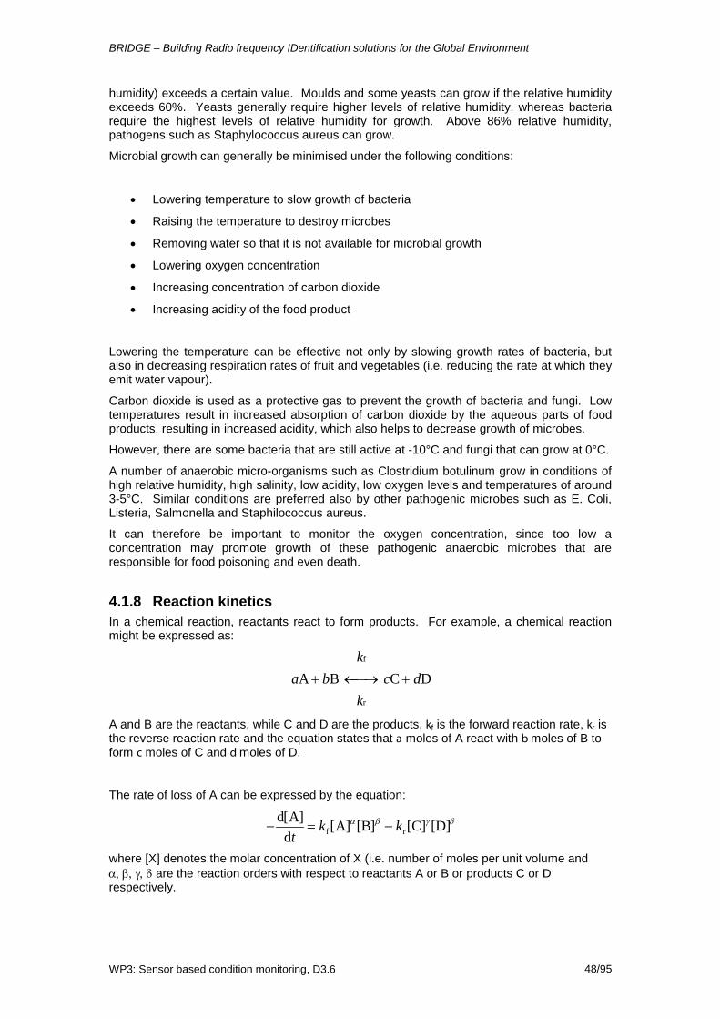
BRIDGE – Building Radio frequency IDentification solutions for the Global Environment
WP3: Sensor based condition monitoring, D3.6 48/95
humidity) exceeds a certain value. Moulds and some yeasts can grow if the relative humidity exceeds 60%. Yeasts generally require higher levels of relative humidity, whereas bacteria require the highest levels of relative humidity for growth. Above 86% relative humidity, pathogens such as Staphylococcus aureus can grow.
Microbial growth can generally be minimised under the following conditions:
• Lowering temperature to slow growth of bacteria
• Raising the temperature to destroy microbes
• Removing water so that it is not available for microbial growth
• Lowering oxygen concentration
• Increasing concentration of carbon dioxide
• Increasing acidity of the food product
Lowering the temperature can be effective not only by slowing growth rates of bacteria, but also in decreasing respiration rates of fruit and vegetables (i.e. reducing the rate at which they emit water vapour).
Carbon dioxide is used as a protective gas to prevent the growth of bacteria and fungi. Low temperatures result in increased absorption of carbon dioxide by the aqueous parts of food products, resulting in increased acidity, which also helps to decrease growth of microbes.
However, there are some bacteria that are still active at -10°C and fungi that can grow at 0°C.
A number of anaerobic micro-organisms such as Clostridium botulinum grow in conditions of high relative humidity, high salinity, low acidity, low oxygen levels and temperatures of around 3-5°C. Similar conditions are preferred also by other pathogenic microbes such as E. Coli, Listeria, Salmonella and Staphilococcus aureus.
It can therefore be important to monitor the oxygen concentration, since too low a concentration may promote growth of these pathogenic anaerobic microbes that are responsible for food poisoning and even death.
4.1.8 Reaction kinetics In a chemical reaction, reactants react to form products. For example, a chemical reaction might be expressed as:
aA + bB kf
← → kr
cC + dD
A and B are the reactants, while C and D are the products, kf is the forward reaction rate, kr is the reverse reaction rate and the equation states that a moles of A react with b moles of B to form c moles of C and d moles of D.
The rate of loss of A can be expressed by the equation:
−d[A]dt
= kf [A]α[B]β − kr [C]γ [D]δ
where [X] denotes the molar concentration of X (i.e. number of moles per unit volume and α, β, γ, δ are the reaction orders with respect to reactants A or B or products C or D respectively.
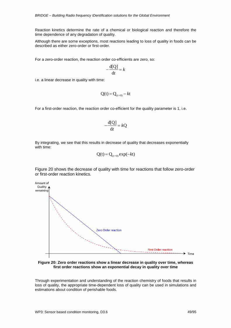
BRIDGE – Building Radio frequency IDentification solutions for the Global Environment
WP3: Sensor based condition monitoring, D3.6 49/95
Reaction kinetics determine the rate of a chemical or biological reaction and therefore the time dependence of any degradation of quality.
Although there are some exceptions, most reactions leading to loss of quality in foods can be described as either zero-order or first-order.
For a zero-order reaction, the reaction order co-efficients are zero, so:
−d[Q]dt
= k
i.e. a linear decrease in quality with time:
Q(t) = Q(t =0) − kt
For a first-order reaction, the reaction order co-efficient for the quality parameter is 1, i.e.
−d[Q]dt
= kQ
By integrating, we see that this results in decrease of quality that decreases exponentially with time:
Q(t) = Q(t =0) exp(−kt)
Figure 20 shows the decrease of quality with time for reactions that follow zero-order or first-order reaction kinetics.
Figure 20: Zero order reactions show a linear decrease in quality over time, whereas
first order reactions show an exponential decay in quality over time
Through experimentation and understanding of the reaction chemistry of foods that results in loss of quality, the appropriate time-dependent loss of quality can be used in simulations and estimations about condition of perishable foods.

BRIDGE – Building Radio frequency IDentification solutions for the Global Environment
WP3: Sensor based condition monitoring, D3.6 50/95
• Condition of perishable foods: Summary The condition of a perishable food product is not a single measure, but rather a combination of measures including aesthetic appearance, texture, flavour, nutritional value. Each of these qualities depends on the degree of freshness of the food since harvesting and the conditions under which it has been handled (during processing, storage and transportation). Depending on the chemical composition and structure of the food product, each will have its own specific vulnerabilities and decay mechanisms and the biological and chemical reactions that cause decay or degradation and their reaction rate kinetics (and hence the speed of the decay) are influenced in turn by environmental factors such as temperature, humidity, concentrations of gases and mechanical damage (e.g. bruising, puncturing). The growth of pathogenic microbes is a particular concern, not only affecting actual and perceived food quality but more importantly, food safety. Lowering of humidity, temperature and pH value, together with the use of modified gas environments can inhibit or slow their growth - so sensors have a role to play in monitoring and detecting the conditions under which such pathogenic microbes could grow, as well as the integrity of any protective environments during transportation or storage.
To develop a contextual model for determining the condition, remaining shelf life and safety of a specific perishable food product, it is necessary to take all these factors into account when choosing what properties to sense and the algorithms that transform the sensor measurements into measures of condition, both in terms of quality (e.g. nutritional value, customer satisfaction) and food safety. There are always a number of anomalies and exceptions, so it is always advisable to consult specialised handbooks on food safety and shelf life.
4.2 Condition of mechanical equipment - vibration analysis Mechanical equipment and machinery with moving parts can be subject to failures, resulting from wear, mechanical strain, unbalancing of loads etc. Data from vibration sensors can be analysed in order to detect the early signs of instability that ultimately lead to failure and breakdown, so that corrective maintenance and repair activity can be undertaken prior to failure [Bogert, 1963] [Meirovitch, 1986] [Newland, 1989] [Norton, 2003]. Condition-based maintenance and health management of assets is becoming an important tool for many organisations, in particular those with high-value machinery or those who are responsible for fleets of assets that require cost-effective servicing and maintenance. In the past, scheduled maintenance activities were performed and parts replaced either at regular time intervals or after a particular number of hours of usage or operational cycles. The lifetime of such parts or time span between such maintenance activities was usually determined to ensure a high probability of uptime or availability of the equipment, but this included a safety margin, since there is a statistical variation in the time to failure of each part or of the machine as a whole. In contrast, condition-based maintenance offers the prospect of being able to only perform maintenance or replacement of parts when it is actually necessary, as a result of continuous or intermittent monitoring of signals such as the noise and vibrations from the equipment. The previous section was concerned with analysis of sensor data that is collected for perishable foods during storage and transit through supply chains. The supply chain context to this work is that monitoring of vibration data can be used as a trigger for planning maintenance activities and ordering of replacement parts, as well as having an impact on the production schedule for products that rely upon the availability of such equipment for their manufacture. A number of techniques can be used for condition monitoring, including monitoring of current and voltage levels for electrical equipment such as motors and pumps, analysis of debris resulting from wear and abrasion. Vibration analysis can be used for continuous of intermittent monitoring of equipment with moving parts. During normal stable operation, the machinery has stable noise and vibration frequency

BRIDGE – Building Radio frequency IDentification solutions for the Global Environment
WP3: Sensor based condition monitoring, D3.6 51/95
spectra. However, as parts become worn, strained or imbalanced, the noise and vibration spectrum changes, generally increasing in amplitude over a relatively short time period prior to failure. A simple approach for analysing data from vibration sensors is to calculate the crest factor, which is the ratio of the peak amplitude to the root mean square (r.m.s.) amplitude. The crest factor can be used to detect impulsive vibrations, such as those produced by damaged bearings when the crest factor exceeds 3.5. By analysing data from vibration sensors in the frequency domain, it is possible to detect subtle changes in the vibration spectrum at a much earlier stage, since it is then possible to detect the increasing amplitude of specific frequency components of the vibration spectrum, relative to other frequency components, even though the increase of those specific components may not be so noticeable in the overall amplitude of the noise or vibration spectrum, when averaged across all frequency components or over time.
Figure 21: By Fourier transforming vibration data to the frequency domain, changes in the amplitudes of specific frequency components can be detected with much greater
sensitivity than by inspection of r.m.s. amplitudes in the time domain
Furthermore, it is possible to use the vibration spectrum in the frequency domain in order to perform fault diagnosis, if detailed knowledge of the machine is available, such as the rotational speed of various axles, number of gear teeth in gearwheels, geometry of bearings etc. Vibration data is often collected using piezoelectric or piezoresistive transducers. These must be positioned appropriately on the machine in order to ensure direct transmission paths to the part being monitored and avoid contamination of the signals with vibrations from other machine parts. Many data samples are collected at closely spaced periodic time intervals and averaging can be used to improve the signal/noise ratio. In order to transform the signal into the frequency domain for analysis, it is necessary to apply a Fourier transform. The classical Fourier transform is defined as:
F(ω) =12π
f (t) e− iωtdt−∞
∞
∫
The corresponding inverse Fourier transform is given by:
f (t) =12π
F(ω) eiωtdω−∞
∞
∫

BRIDGE – Building Radio frequency IDentification solutions for the Global Environment
WP3: Sensor based condition monitoring, D3.6 52/95
In practice, the data that is sampled is not collected between infinite time intervals in the past and future, but within discrete time intervals or windows. This means that effectively the data that is being transformed is the multiplicative product of the infinite data series and a 'top-hat' function corresponding to the sampling window. Because the Fourier Transform of a product of two function is the convolution of their separate Fourier Transforms, the result of sampling within a time window is that the ideal frequency spectrum is convolved with a sinc function (sinc(x) = sin(x) / x) that is the Fourier Transform of the 'top-hat' window function. As shown in Figure 22, the larger the time window, the narrower the width of the sinc function and therefore less 'blurring' of the true frequency spectrum.
Figure 22: A sampling window spanning a time period T is transformed into a sinc
function whose width is inversely proportional to T
Another distortion effect results from the discrete periodic sampling rate. In this case, the sampled data is effectively the product of the true signal multiplied by a periodic array of delta functions, separated in time by the sampling period. Again, because the Fourier Transform of a product is the convolution of the Fourier Transforms of each of the two signals that are multiplied together. As shown in Figure 23, the Fourier Transform of an infinite periodic array of delta functions with period ∆T is an infinite periodic array of delta functions with spacing 2π/∆T. This leads to an effect known as aliasing, which places a limit on the frequency range that can be analysed for a given sampling rate.
Figure 23: A sampling function or Dirac comb of delta functions with temporal spacing
∆T is Fourier transformed into another Dirac comb, with spacing 2π/∆T
Therefore, when a vibration signal is sampled for a finite time period T, with samples being taken periodically with period ∆T, the sampled signal is the original signal, multiplied by a top hat function of width T, multiplied by the periodic array of delta functions with temporal spacing ∆T. The resulting Fourier transform of the sampled signal will be the Fourier transform of the true signal, convolved with the sinc function, convolved with the array of delta functions with frequency spacing 2π/∆T. The larger the sampling window T and the smaller the sampling period ∆T, the closer the Fourier transform of the sampled signal is to the Fourier transform of the true signal. Digital computing technology allows Fourier Transforms to be calculated efficiently using Fast Fourier Transforms (FFT). The FFT algorithm significantly reduces the number of computing operations required.

BRIDGE – Building Radio frequency IDentification solutions for the Global Environment
WP3: Sensor based condition monitoring, D3.6 53/95
Vibrations seldom consist of pure sinusoidal waveforms, so harmonics can arise, typically at multiples of the fundamental frequency. For example, the Fourier Transform of a square wave waveform consists not only of the fundamental frequency but also harmonics at odd integer multiples of that frequency, i.e. 3f0, 5f0, 7f0, etc. It can be useful to analyse the relative strength of harmonics in relation to the fundamental frequencies, since this can also be an indication of instability that might lead to breakdown. Techniques known as power cepstrum analysis and complex cepstrum analysis can be used for investigating periodicity in the frequency spectrum, just as Fourier Transforms can be used for investigating periodicity in the time-based vibration data. The power cepstrum is the inverse Fourier transform of the logarithm of the power spectrum of a signal. It can be used to identify periodicity in the frequency spectrum, as well as the detection and removal of echoes from the vibration spectrum. The complex cepstrum is the inverse Fourier transform of the logarithm of the forward Fourier transform of the time-dependent signal, x(t). It can be used for deconvolution of a signal in the quefrency domain, then transformation back to the time domain. This is possible because the complex cepstrum contains information about the magnitude and phase of the signal. Other techniques that can be used for vibration analysis include auto-correlation and cross-correlation methods, as well as dual signal analysis. Dual signal analysis is useful for identifying and ranking different transmission paths for vibrations by analysing the time delay between closely correlated signals. Impulse-response functions can be used to determine the structural modes of vibration of a complex structure or machine. Typically an impulsive input (such as a hammer containing a calibrated force transducer) is used to strike the object - and the vibration sensors record the transient output response. Dual signal analysis is used to calculate the impulse-response function of a particular object or system. From this brief summary, it is apparent that digital signal processing of data from vibration sensors can be used to detect early signs of imminent failure and can even be used to analyse the root cause of the defect that is causing the instability. Further discussion on techniques for analysing vibration data are outside the scope of this deliverable, although the reader is advised to refer to various textbooks on vibration analysis for further details, including case study examples on particular kinds of mechanical equipment and couplings. It is by now apparent that condition of a mechanical part or machine is not something that is trivially or linearly related to the raw output of a vibration sensor, but rather that it is something that can be determined through mathematical analysis of the data, together with detailed knowledge of the design and normal angular speeds of rotating, oscillating or reciprocating parts within the machine. As mentioned earlier, this discussion of analysis of vibration data focuses on its use as an early warning mechanism for imminent failures, such that it can be used as a trigger for supply chain operations that need to happen in order to avoid disruption, by scheduling condition-based maintenance, ordering of spare parts likely to be required (especially if there is a long lead time), as well as adjusting production schedules to anticipate downtime and non-availability of the machinery at least during the planned maintenance operations. Having said that, there are reports of detrimental effects of low-frequency vibrations on perishable goods - so there can be a case for also monitoring the shocks and vibrations of goods during transportation.

BRIDGE – Building Radio frequency IDentification solutions for the Global Environment
WP3: Sensor based condition monitoring, D3.6 54/95
5 Condition Monitoring Analytical Studies
5.1 Value of Sensor Information for the Management of Perishable Goods
As mentioned in Section 4, the lifetime of perishable goods is influenced by environmental conditions such as temperature, relative humidity, and shock. Sensors can monitor these parameters and enhance logistic decision-making based on the actual quality level of goods. In this simulation study we will show that a sensor based approach is superior to established practices even when considering the abilities of individuals to judge the goods’ quality by visual and tactile inspections. With sensor information, retailers can achieve higher profits, increased resource efficiency, higher quality, and a reduced amount of perished goods on the sales floor.
5.1.1 Background Perishable goods such as fruits, fresh cut produce, meat, and dairy products are of utmost importance for the retail grocery business. Not only are perishables a major direct source of revenue as they account for over 50 percent of the $400 billion annual turnover of the US retail grocery industry [First , 2005]. Their availability, presentation, and perceived quality even appear to be more important to consumers’ store choice than the availability of branded products [Goldman, 2002] [Krider, 2000] [Tsiros, 2005], only exceeded by the factors store cleanliness and price. In fact, the importance of perishable goods for the retail sector has been widely accepted. Their management, however, constitutes a severe challenge for retailers and their supply chain partners alike. Improper storage, transport, and handling conditions often result in unsellable products and lead to out-of-stock situations. The impact of inefficient management of perishables also becomes apparent on a broader economic scale. For instance, ten million tons or ten percent of the total industrial and commercial waste in the UK [DEFRA, 2007] are caused by perishable food products. Putting these figures into relation with average grocery margins of two to six percent [DEFRA, 2006] illustrates the potential of improving profitability by reducing waste. Beyond profitability, the ecological side effects of the food supply are of major concern as well. Between 20 and 30 percent of the carbon dioxide equivalent emissions in Europe are caused by producing, transporting, preparing, and storing perishable food products [EU, 2006]. Cutting down the wastage of such goods therefore constitutes a considerable leverage for reducing the emission of greenhouse gases. The limited lifetime and the deteriorating quality of perishable goods over time contribute greatly to the complexity of their management. The major challenge, however, stems from the dependency of the remaining lifetime and quality on environmental factors such as temperature, relative humidity, and shock. In most supply chain operations, these factors are difficult to control. Even if the products are distributed using carefully designed state-of-the-art processes, variations in environmental conditions occur that often lead to quality drops [Sloof, 1996]. These quality drops may only affect parts of the shipment, which are either caused by temperature changes in certain areas of a container, often referred to as micro-climates, or due to vibrations of different amplitude depending on the placement of a palette within the consignment. Consequently, even shipments which have the same best before date and leave the producers with a homogeneous level of quality may arrive at the retailer with different quality levels. The variations are often difficult to assess by merely visual or tactile inspections. Perceptible changes in colour and consistency mostly become apparent only during the later stages of a product's life

BRIDGE – Building Radio frequency IDentification solutions for the Global Environment
WP3: Sensor based condition monitoring, D3.6 55/95
(i.e. mostly on the sales floor), and therefore human-sense-based examinations are hardly able to aid decision making with respect to the future distribution of products. As a result, inherent supply chain problems are often not recognised when they occur, deficient shipments are further processed as planned even if the product will be spoilt before reaching the end-customer, and products on the sales floor cannot be arranged in an optimal way with respect to their remaining shelf life. While the human senses have only a limited capability to assess the intrinsic product properties, modern sensor technologies can help to provide the required information. Tracking environmental parameters such as temperature and vibration for individual logistic units allows problems in the supply chain to be spotted and the actual quality levels of individual products to be more precisely predicted [Sahin, 2007], all of which aids the decision making with respect to the future distribution of products. As the costs of sensor and communication technologies have decreased dramatically over the last decade, electronic quality monitoring techniques have become attractive to a wider range of supply chain applications. The value of such approaches with respect to the management of fast moving perishable goods, however, is not yet fully clear. Therefore, the goal of this study is to compare a sensor-based management approach of perishable goods with a widely established process based on perceptible quality changes by consumers and employees. We use a computer simulation method to explore and quantify the value of sensor information in a typical retail supply chain. We optimize both the traditional and the sensor-based approach for profit and measure the respective resource efficiency dependent on several supply chain, product, and user parameters.
5.1.2 Literature Review Topics related to the management of perishable goods are frequently addressed in management research. In the context of this study, key aspects are issuing policies and, in the broader sense, quality models for perishable goods. We provide a brief overview of the most relevant contributions below. In his comprehensive literature review [Nahmias, 1982] outlined several streams of research in the field of perishable inventory theory. He grouped the research streams into the two fields of ‘fixed-life perishable inventory’ and ‘continuously deteriorating inventory’. An important finding was that the fixed-lifetime assumption of perishable goods according to which all goods are “equally fresh” on arrival should be replaced by a more realistic hypothesis. Nahmias suggested describing the lifetime with a general life-time function instead, and argued that the investigated issuing policies were limited to Last-In-First-Out (LIFO) and First-In-First-Out (FIFO) approaches due to the focus on the fixed-life perishable problem. Both types of policies are time-based strategies which prioritize items according to the total elapsed time (i.e. age) that an item has been in storage regardless of the goods’ actual quality conditions. The literature reviews of [Raafat, 1991] and later [Goyal, 2001] showed that researchers picked up the challenges proposed by [Nahmias, 1982]. Raafat, Goyal, and Giri recognized a shift from the previously dominant fixed-life perishable inventory publications towards the area of continuously deteriorating inventory. [Wells, 1989] were among the first to publish an issuing policy based on the actual quality of an item. Motivated by temperature-aware chemical sensors, so-called Time-Temperature Indicators (TTI), they developed a type of Shortest-Remaining-Shelf-Life (SRSL) issuing policy. Their policy took into account that every individual item can have a different deterioration history and thus a different remaining shelf life. They conducted computer simulations and showed that for frozen goods the SRSL policy outperformed LIFO and FIFO policies. The results outlined the value of sensor-based strategies for the special case of frozen goods. In contrast to most fresh perishable goods, frozen goods do not show quality changes that can be easily evaluated by visual and tactile inspections. Therefore, Wells and Singh left the
BRIDGE – Building Radio frequency IDentification solutions for the Global Environment
WP3: Sensor based condition monitoring, D3.6 56/95
abilities of employees or consumers unconsidered that allow them to roughly estimate the quality of at least some products. In order to demonstrate how valuable the actual quality information of products is for a supply chain, [Ferguson, 2006] studied an example where a supplier shared the actual stock-age distribution with a retailer to reduce the number of low quality items. By using this information, it was possible to optimize the replenishment behaviour of the simulated retailer and thereby its profit. While their work included several extensive analyses covering different issuing policies and demand sensitivity to product freshness, they, similar to Wells and Singh [Wells, 1989], did not take into account that consumers and employees could possess at least a limited ability to make decisions based on perceptible quality features. In contrast, our model optimizes the flow of goods with regard to the difference between actual and perceptible quality changes. A publication that took the consumer’s perspective into account is the work of [Vaughan, 1994]. He investigated a scenario where consumer-realized product expiration in-store or shortly after a purchase had a negative impact on a retailer’s profit that far exceeded the loss from stock-outs. He treated the age at which a vendor outdates a product as a decision variable and showed that, by a suitable choice thereof, the consumer experience could be improved. However, the optimisation of Vaughan is focused solely on the retail store level and thus has no impact on improving logistic decisions at an earlier stage, which can be used to prevent the unnecessary distribution of low quality items to the store. Though [Osvald, 2008] did not investigate issuing policies for perishable goods, their work is also relevant for this study as they were among the first to utilize the difference between actual and perceptible quality changes in a perishable supply chain context. A major finding was that this approach offered new possibilities to prevent products from perishing. Their solution for a routing problem decreased the unnecessary time products spent in vehicles and thus reduced the number of perished items. To the best of our knowledge, no paper has been published which studies the value of sensor information while taking into account the consumers’ or employees’ abilities and behaviour based on the perception of visual quality features of products. We have developed a simple heuristic for a two-level supply chain consisting of a supplier and retailer that reduce the number of in-store perished goods and increase profit. In our model, we consider a continuous (s, S) ordering policy with fixed and variable costs and positive lead-times. We compare a sensor-based solution with a traditional approach under the two important issuing policies of selecting expiring products or freshest products first. Against this background, we aim to extend the existing body of knowledge in the following four ways. We provide 1) heuristics that can be applied in practice for nearly all perishable products, 2) a quantitative analysis of the value of sensor information for the management of perishable goods based on simulation studies, 3) a full sensitivity analysis of our approach, and 4) a discussion of the impact of our findings on the retailer/supplier relationship.
5.1.3 Analytical Studies
5.1.3.1 Simulation model Base case parameters and the supply chain configuration stem from a research project with a major Swiss retailer. The basis for our analysis is a typical setting in the retail industry. A retailer with inventory I sells a perishable product at price cp to consumers and receives replenishments from a larger supplier. As Figure 24 shows, the supplier ships the goods to the retailer’s local distribution centre where they are transhipped and delivered to their final destination, the retail store. During the

BRIDGE – Building Radio frequency IDentification solutions for the Global Environment
WP3: Sensor based condition monitoring, D3.6 57/95
transhipment, employees at the local distribution centre pre-sort the consignment according to the issuing policy used at the retail store. In practice, no additional personnel are required because the pre-sorting could simply be achieved during the picking operation by means of an additional sort parameter on the picking list. For each delivery step, we assume a positive lead-time of l1 and l2, respectively. The product of interest is a short life perishable commodity, which leaves the supplier with an initial quality level M. A product is outdated once its quality level falls below a threshold CAQ. At the beginning of each simulated day, a routine check is performed at the retail store to remove outdated products and to adjust the inventory records accordingly. Consumer demand at the retail store is discrete and follows a Poisson distribution with rate of λ per period. Demand is directly satisfied from the retailer’s stock. Unmet demands are lost. The retailer’s stock is replenished according to a continuous (s,S) replenishment policy. Each replenishment order incurs fixed costs cK and purchasing costs cW per ordered item.
Figure 24 The model of the simulated supply chain
We assume that replenishments from the supplier to the retailer’s local distribution centre are exposed to fluctuating environmental parameters caused by micro-climates, temperature variations, and shock that affect the quality levels of the items in the consignment. The disturbances do not affect all the items of a load equally [Dabbene, 2008], [McRoberts, 2003]. As a result, the variability in the distribution of the quality levels increases. To account for these characteristics, we assume that during each day of transport the quality level of each individual item is randomly dropped according to an exponential distribution with mean μq. We refer to this function as the quality drop function. In order to differentiate between the effects of stock-aging at the supplier’s end and quality drops during transport or handling, we assume that the supplier has ample capacity and composes its shipments of fresh goods with the maximum quality level M. Note that with stock aging at the supplier’s end, the variability of the quality level distribution would be even greater. Table 10 summarises all parameters and variables used in our simulation. For our experiments, we compare two different scenarios. In the first one, temperature data about the products is not gathered and therefore employees must base their decisions on discernible visual changes of the individual items. We refer to this scenario as the “classical approach”. In the second scenario, sensors attached to transport cases (i.e. reusable plastic crates) record temperature deviations and therefore allow decisions based on effective quality levels of products to be made. Employees can use this information to make informed decisions beyond their visual capabilities. At the local distribution centre, they pre-sort the items according to the actual quality level. In addition, a heuristic determines how many cases of the shipment should be delivered to the retail store or should be discarded immediately because of an overly low quality. We refer to this scenario as the “sensor-enhanced approach”.
Table 7 Variables and parameters used in the simulation

BRIDGE – Building Radio frequency IDentification solutions for the Global Environment
WP3: Sensor based condition monitoring, D3.6 58/95
Reorder level Order-up-to level
Number of simulation runs Duration of a simulation run [d]
Initial quality level of products leaving the supplier stock Mean consumer demand per period Transport time from supplier to distribution centre Transport time from distribution centre to retail store Selling price per item Purchasing costs per item Retail margin One period holding costs per item at the retail level Fixed costs per order Mean of quality drop function
Minimum customer accepted quality level Maximum discernible quality level
Total number of sold items per simulation run Total holding amount per simulation run (VIW + VDW) Total amount of waste per simulation run Total number of replenishments per simulation run
5.1.3.2 The Model for Quality Loss and Consumer Perception Without sensor technologies, the quality level of a product can still be estimated by its discernible visible6 features. The assumption that employees and consumers treat all
instances of a product the same regardless of their visual appearance would introduce a bias towards the sensor-enhanced approach. Thus, the baseline for our investigation
is a more realistic quality loss model, such as used by [Osvald, 2008], in which consumers and employees have limited abilities to reason about the quality level of a
product depending on the product characteristics. In the quality loss model, a perishable product has a maximum lifetime only under optimal environmental
conditions. The lifetime is divisible into two phases (cf.
Figure 25Figure 25). At point t = 0 the product has the highest quality. During the first phase t ∈ [0,A], the actual quality is decreasing, but with no discernible changes to a consumer or an employee. When the quality level falls below the maximum discernible quality level α, noticeable changes (at point A) start in one or more of the quality parameters. During the second phase t ∈ [A,B], the changes continue up to point B. Beyond point B, the product becomes unsellable and must be discarded without any salvage value. The biggest potential for optimisation based on sensor
6 For simplicity, we do not include other inspection types such as taste, smell, etc. in this study.

BRIDGE – Building Radio frequency IDentification solutions for the Global Environment
WP3: Sensor based condition monitoring, D3.6 59/95
information is therefore in the area of t ∈ [0,A] where any changes in, for example, the order of issuing will be invisible to the consumer’s eye.
Figure 25 An illustration of the quality loss model showing the difference between
effective and visible quality (adapted from [Osvald, 2008])
In our simulation model, consumers base their buying decisions on the previously illustrated quality loss model. To account for different consumer needs and marketing strategies, we apply our heuristics with respect to the two most important quality-based issuing models, namely the Highest-Quality-First-Out (HQFO) and Lowest-Quality-First-Out (LQFO) policy, which are the quality-based counterparts of the time-based issuing policies Last-In-First-Out (LIFO) and First-In-First-Out (FIFO). In the HQFO policy, consumers always pick items with the highest quality first. A typical example of where a HQFO policy is used is in bagel stores, where fresh items are sold first. Only if all the fresh items are depleted, bagels from the previous day are used to satisfy the demand. In the LQFO policy, consumer demand is satisfied with items of the lowest quality first. Typical examples are “load-from-the-back” shelves, such as those used for fresh cut produce/salad, where consumers are forced to pick items in a certain order. While consumers are able to distinguish the quality of products in t ∈ [A,B], products in t ∈ [0,A] will be perceived as having the same high quality. By using sensors attached to reusable transport crates, the difference between effective quality and visual quality in t ∈ [0,A] can be exploited to increase the resource efficiency (and thus the profit), while retaining the same high quality level from the consumer perspective.
5.1.3.3 Sensor-aware Heuristic The sensor-aware heuristic optimizes the operations at the retailer’s distribution centre by 1) removing items of an overly low quality and 2) by pre-sorting an incoming shipment according to the selected issuing policy at the retail store. In the following, we provide definitions relevant for the description of these two steps. Let G(t) = {1,2,…,X} denote an incoming shipment at time t which contains |G(t)| = X items. The first elements of G(t) will be issued first to a consumer. Based on the previously described quality loss model, ex(t) denotes the effective quality of an item x at point t and vx(t) the visible quality of an item x at point t. The time at which an item x leaves the supplier is expressed by sx. At sx, every item has the initial quality level M, which decreases over time at rate a. The maximum discernible visible quality is denoted as V. The quality drop that affects items between the supplier and the retailer’s distribution centre is defined as d. With these definitions, we can describe the effective quality of a specific item for any given time with the following functions:
( 2 )
The visible quality of an item x at time t is therefore defined as:

BRIDGE – Building Radio frequency IDentification solutions for the Global Environment
WP3: Sensor based condition monitoring, D3.6 60/95
( 3 ) The first step is to remove those items of an overly low quality. We consider items to have an overly low quality if they are below the sellable quality level CAQ. This condition can be violated 1) already at the distribution centre or 2) at the arrival time at the retail store. With l2 being the lead-time from the distribution centre to the retail store, the items that should be further shipped are defined as: ( 4 )
The second step of our heuristics is to pre-sort the remaining items of the shipment to optimize the order with respect to the selected issuing policy at the retail store. For this simulation study, we investigate LQFO and HQFO issuing policies. In general, the LQFO case is preferred by retailers as items with the lowest quality get sold first and thus fewer items expire. For the LQFO case, all the elements x of G’(t) are sorted in ascending order by their effective quality ex(t). However, as consumers often demand items with the highest quality, the HQFO case is equally important. While retaining the consumers’ perceived quality, we can utilize the sensor information to optimize the area beyond the maximum discernible quality level for the retailer. To achieve this goal, we divide G’(t) into two different sets G’1(t) and G’2(t) with G’1(t) ∪ G’2(t) = G’(t). The sets can be described by the following equations: ( 5 )
The set G’1(t) contains all the items whose quality on their arrival at the retail store can be distinguished by a consumer, G’2(t) contains the remaining items whose quality is so high that a consumer could not detect any differences. While the HQFO policy implies that we have to sort G’1(t) in descending order of quality levels, consumers will experience no difference if we change the order in the set G’2(t) to an ascending order, which is better for the retailer.
While the sensor-aware operations can base the sorting and removal decisions on the effective quality of items ex(t), employees and consumers can only rely on the visible quality
vx(t) of items. To illustrate the previously described sorting heuristics, we consider the following example of a HQFO case, where a shipment was exposed to temperature variations
and has the discrete, unsorted quality values as depicted in the first line of Figure
26
Figure 26. With a maximum discernible quality level MDQ = 2, employees are able to achieve the sorting results illustrated in the second line. While the items on the left can easily be sorted, the remaining four items are still in random order as an employee will perceive them as being of the same high quality. With sensor information, the employees know the effective quality. Thus, the order can further be optimised.

BRIDGE – Building Radio frequency IDentification solutions for the Global Environment
WP3: Sensor based condition monitoring, D3.6 61/95
Figure 26 An example of sorting in a HQFO policy by visible quality features only, or by utilizing sensor data for a maximum discernible quality level of two
In the following, we put the heuristics into action by simulating the scenarios of sensor-based versus classical approaches to satisfy consumer demands according to the selected issuing policy.
5.1.4 Simulation Results
5.1.4.1 Base case analysis The base case for our simulation studies is a fresh, short life commodity (such as strawberries) with an initial quality level M of eight points at the supplier level and daily demand of six trade units per day at a selling price cp of $24 per trade unit (each trade unit consisting of twelve sellable consumer units at $2). The purchasing price cw is $12 per trade unit, which corresponds to a retail margin cm of 50 percent. In addition, fixed replenishment costs ck of $12 per order occur. Both transport lead-times l1 and l2 are set to one day. Due to temperature variations during loading at the supplier’s end, transport from the supplier to the distribution centre, and unloading at the distribution centre, the effective quality level of each product is assumed to have randomly dropped according to an exponential distribution with mean μq = 0.75 days. Holding costs ch per unit per day are set to $1 for the retail store. We measure the performance of our heuristics by using the profit function of equation6. For one simulation run, VS is the number of sold items, VH the holding amount, VR the number of replenishments, VIW the number of perished goods at the store level (in-store waste), VDW the number of removed items at the distribution level (distribution waste), and VW = VIW + VDW the total amount of waste. Note that we assume no penalty for perished goods other than the lost margin. ( 6 )
The simulations were executed on a high performance cluster and written in the Python programming language. In our simulation program, the classical and the sensor-enhanced scenarios were compared with the same parameters for a simulated time of 600 days and N=100 replications. The first 100 days were removed as a warm-up period according to the method outlined by [Law, 2001]. Thus, the simulated time T equalled 500 days. For variance reduction, the widely recommended and used common random number (CRN) approach was applied to both the demand arrivals distribution and the quality drop distribution. With a search over 0 < s ≤ S ≤ 40, the optimal values for (s,S) with respect to profit were determined. In the following, M1* denotes the optimal found configuration for the classical approach, whereas M2* denotes the optimal found configuration for the sensor-enhanced approach. We explore the cases of LQFO and HQFO separately.
Table 8 A base case comparison of the classical approach (M1) versus the sensor-enabled approach (M2)
LQFO HQFO M1* M2* Change M1* M2* Change ( ) (22, 32) (22, 32) (20,29) (20,29)

BRIDGE – Building Radio frequency IDentification solutions for the Global Environment
WP3: Sensor based condition monitoring, D3.6 62/95
Profit 25541 25976 +1.70% 20345 21730 +6.81% Sold units 2861 2875 +0.49% 2588 2639 +1.97% Holding amount 4524 4633 +2.41% 3218 3350 +4.10% Total waste 88.6 58.2 -
34.31% 335.9 262.0 -
22.00% In-store waste 88.6 29.3 -
66.93% 335.9 241.7 -
28.04% Replenishments 267.18 265.87 -0.49% 288.31 287.11 -0.42% Perceived quality 1.5814 1.6449 +4.02% 1.8705 1.9160 +2.43% Effective quality 2.0467 1.9677 -3.86% 2.7804 2.6290 -5.45% OOS 4.80% 4.34% -9.58% 13.89% 12.18% -
12.31% Table 8 shows the results and averaged performance metrics for the simulation runs. The profit increase of the sensor-based approach over the classical approach amounts to 1.70 percent in the LQFO and to 6.81 percent in the HQFO case. The 99 percent confidence interval for the mean profit increase is 0.2 percent in the LQFO case and 0.46 percent in the HQFO case. As Table 8 shows, the profit increase is based mainly on the decreased number of unsellable goods (-34.31 percent for LQFO and -28.04 percent for HQFO) and the decreased number of out-of-stocks (-9.58 percent for LQFO and -12.31 percent for HQFO). This confirms that the sensor-based approach is more resource efficient than the traditional approach. As fewer products are thrown away, the holding costs rise slightly as the retail shelf space is better utilized. From a consumer’s perspective, the shopping experience is improved considerably. Although the effective quality decreases, the quality perceived by consumers increases by 4.02 percent in the LQFO and 2.43 percent in the HQFO case respectively. Moreover, in-store waste which could have a negative impact on consumers is dramatically reduced. By intelligent sorting and the removal of only 0.9 percent in the LQFO case (0.07 percent in the HQFO case) at the distribution level, the amount of in-store waste decreases by 66.93 percent in the LQFO case (by 28.04 percent in the HQFO case). In conclusion, the sensor-based approach achieved its goal of increased resource efficiency while at the same time improving the consumer experience and reducing the amount of in-store waste. While the sensor-based approach yields additional profit, it also induces additional costs. In our simulation, we focus on improving a process for a single product of a retailer. We assume that the fixed infrastructure for reading sensors is already installed for use with multiple products and also multiple sensor-based applications. Thus, the primary cost driver for a deployment of our proposed sensor-based approach is sensor costs. Sensors with temperature logging capabilities are available as semi-active RFID tags with a battery lifetime of three to six years (depending on the logging interval). An initial investment is needed to equip enough existing reusable logistic items with temperature logging sensors. Sensor costs are denoted as cS. For the base case, we need approximately 50 reusable logistic units equipped with sensors, which translates into an initial investment of C0 = 50 * cS. As sensors may be damaged during operations, we assume a replacement rate of 20 percent/year, which translates into yearly costs of Cy = 20% * C0. With a targeted ROI in three years, we get the following results with a Net Present Value (NPV) calculation7
7
for the maximum allowable sensor costs. For the LQFO case, costs per sensor may be up to $16.29, while in the HQFO the costs per sensor may be up to
, where represents the annual interest rate of eight percent.

BRIDGE – Building Radio frequency IDentification solutions for the Global Environment
WP3: Sensor based condition monitoring, D3.6 63/95
$51.86 to achieve a ROI in three years. Considering current market prices for temperature logging sensors (about $15 to $25), the proposed sensor-based approach seems feasible from a cost perspective.
5.1.4.2 Sensitivity Analysis The sensitivity analysis allows us to investigate the applicability of our results to a wide area of different scenarios beyond the base case by choosing different parameter values. We conducted a set of experiments that comprised a full factorial design for all combinations of the following parameters:
As we explored LQFO and HQFO policies separately, our sensitivity analysis comprises a total of 2 * 3645 = 7290 design points. For each design point, we searched for the profit-wise optimal (s,S) replenishment parameters for M1 and M2. Each experiment was replicated ten times with different random number initialisations based on the CRN technique. Thus, our sensitivity analysis comprised a total of 12,355,200 experiments.Table 9 reports the average results across all experiments for each fixed parameter value and with respect to the selected issuing policy. We show the increase in profit when using the sensor-supported heuristics M2* relative to the traditional approach M1* (cf. Equation 7). Following the framework of [Ketzenberg, 2007], we refer to this measure as Value-of-Information (VOI). The VOI is defined as follows:
( 7 )
The individual rows can be interpreted as follows: the selected parameter value is fixed, while all combinations of the remaining parameters are allowed. Each measure represents the average value of the resulting design points. For example, setting the consumer demand parameter to a value of six units per day results in a VOI of 3.6 percent in the LQFO and a VOI of 3.9 percent in the HQFO case. Columns four to six explain how selected dependent variables contribute to the VOI. The variable ΔVS hereby represents the increased sales revenue, ΔVIW the cost reduction for avoided in-store waste, and ΔVW the total additional costs for perished and removed items compared with the classical approach. We briefly discuss the effect of individual parameter changes below.
Table 9 The results of the sensitivity analysis
LQFO issuing HQFO issuing Parameters
Values VOI VOI
Demand
4 3.6%
1.3% 7.3%
0.9% 3.9% 5.4% 5.5%
-0.5%
6 2.5%
1.4% 5.1% 0.5% 3.5% 3.0% 4.6% 0.5
%
8 1.9%
1.1% 3.8% 0.3% 2.1% 1.0% 4.1% 0.9
% Maximum discernible quality level
0 7.6%
3.6% 7.2% 2.5% 6.8% 3.0% 7.2% 2.5
%
1 3.3%
1.2% 5.3% 0.9% 4.2% 3.0% 4.9% 1.1
%

BRIDGE – Building Radio frequency IDentification solutions for the Global Environment
WP3: Sensor based condition monitoring, D3.6 64/95
2 1.1%
0.6% 4.3% -
0.1% 2.3% 2.8% 4.0% 0.2%
3 0.5%
0.5% 4.0% -
0.3% 1.0% 2.4% 3.5%
-0.4%
max 0.2%
0.5% 3.9% -
0.4% 0.0% 1.2% 2.7%
-0.5%
Quality drop
0.50 1.3%
0.2% 1.9% 0.7% 1.9% 1.1% 1.9% 0.9
%
0.75 2.6%
1.5% 5.1% 0.5% 3.1% 2.6% 4.7% 0.7
%
1.00 3.7%
2.3% 8.5%
0.3% 4.0% 4.4% 8.1%
-0.3%
Initial quality level
7 3.6%
2.4% 8.6%
0.1% 3.9% 4.5% 8.1%
-0.4%
8 2.4%
1.1% 4.5% 0.7% 3.0% 2.4% 4.1% 0.6
%
9 1.6%
0.5% 2.4% 0.7% 2.1% 1.3% 2.5% 1.0
%
Lead-time
1 0.6%
0.1% 0.5% 0.4% 1.2% 1.2% 0.8% 0.7
%
2 2.4%
0.8% 3.3% 1.0% 3.5% 2.2% 3.5% 1.4
%
3 5.7%
3.8%
15.0% -
0.2% 5.8% 6.2% 15.7%
-1.6%
Retail margin
0.25 7.1%
5.8%
18.9% 1.0%
6.4% 18.0% 18.9%
-5.0%
0.50 2.8%
1.1% 5.7% 0.8% 4.0% 3.4% 5.3% 0.8
%
0.75 1.6%
0.6% 2.4% 0.3% 2.0% 0.5% 2.7% 0.9
%
Fixed ordering costs
6 1.6%
0.9% 4.2% 0.3% 2.1% 1.7% 4.1% 0.4
%
12 2.5%
1.2% 5.0% 0.5% 3.0% 2.6% 4.6% 0.6
%
18 3.4%
1.7% 5.6% 0.7% 3.7% 3.4% 5.0% 0.6
% As one may expect, the VOI increases when the maximum discernible quality decreases. When the maximum discernible quality level is set to zero, employees and consumers cannot distinguish the quality of any items. Thus, the VOI is high and reaches 7.6 percent for the LQFO and 6.8 percent for the HQFO case. When the maximum discernible quality level is set to maximum, employees and consumers can easily distinguish the quality difference between one item and another one. The VOI is hereby only achieved by the removal of items with an overly low level of quality at the distribution centre and averages 0.2 percent for the LQFO case and 0.0 percent for the HQFO case. The removal of items at the distribution centre corrects the

BRIDGE – Building Radio frequency IDentification solutions for the Global Environment
WP3: Sensor based condition monitoring, D3.6 65/95
inventory position faster and thus implies a faster replenishment, which leads to increased sales ΔVS by avoiding stock-outs. Another parameter which is related to the uncertainty between effective and visual quality is the mean of the quality drop function. As the mean increases, the impact of random quality drops becomes more pronounced. The more products are affected by micro-climates, shock, etc., the more valuable is the sensor information to estimate their effective quality. For a quality drop mean of 0.50, the VOI equals 1.3 percent and for a mean of 1.0 the VOI equals 3.7 percent in the LQFO case. The values for the HQFO case follow the same correlation, but are generally higher due to the increased sales in comparison to the classical approach. The initial quality level (i.e. the quality level when leaving the supplier) has a strong but easy to explain effect on the utility of the heuristic. A reduction in the initial quality level from nine to seven leads to a clear profit increase from 1.6 percent to 3.6 percent in the LQFO case. The main reason is that short-life products are more sensitive to uncertainties in product lifetime, and the quality level of such products is more likely to fall below the sellable threshold where they cannot be sold at the retailer. More products are likely to perish on the sales floor, and discarding them at the distribution centre (i.e. selecting only the freshest for delivery) reduces in-store waste and out-of-stocks at the retailer. It also reduces ordering costs since the pre-selection leads to longer average shelf life and bigger replenishment lot sizes. Consequently, higher initial quality levels reduce the benefits of the heuristic. These observations are in line with the fact that the characteristics of perishability can be neglected given a long product lifetime (i.e. an extremely high initial quality level). Combining the previous line of arguments is helpful to understand the effect of changes in lead time from the supplier to the distribution centre. The longer the shipment procedure takes, the more likely quality drops are (which are assumed to occur independently from previous events), thus reducing the average time to life and its variance. The latter – under the assumption of independency among the events – reduces the value of the heuristics as assumptions on the actual quality level are more likely to be valid, and sensor data becomes less important8
The demand rate influences the average time a product remains on a shelf before it eventually gets sold. Increasing the demand reduces the average required quality level of a product. Predictions about the remaining quality become less important as the products are more likely to be sold before they go off. Consequently, the relative profit gain of the sensor-aware heuristic decreases with growing demand. Interestingly, due to the sensitivity of the sales increase in the HQFO case, the VOI is higher in comparison to the LQFO case.
. However, this effect is overcompensated by the reduction of the goods’ quality levels when arriving at the distribution centre, which has the same implication of a reduced initial quality level as discussed before. Consequently, the VOI increases in correlation with the lead-time. For the LQFO case, the VOI amounts up to 5.7 percent and up to 5.8 percent for the HQFO case.
Instead of varying the sales price and wholesale price separately, we look at the margin per item. As expected, the value of the sensor based heuristics increases with a decreasing margin as more products have to be sold to compensate for one perished item. The effects of changes to the fixed ordering costs are also well reflected by the simulation results. Higher cost per order forces the retailer to reduce the replenishment frequency and buy in larger quantities. The average time that products
8Assuming that quality drops were more likely for a given consignment when a previous quality drop had occurred (e.g. when a consignment is placed far away from an air conditioner throughout the shipment), this would further increase the value of the sensor-aware heuristics.

BRIDGE – Building Radio frequency IDentification solutions for the Global Environment
WP3: Sensor based condition monitoring, D3.6 66/95
remain on the shelf increases, and the pre-selection at the distributor’s end becomes more important. With the sensitivity analysis, we have explored the correlation between several parameters on the VOI. On average, the profit increase against the classical approach is 2.5 percent for the LQFO and 2.9 percent for the HQFO case.
5.1.5 Summary We have quantified the value of sensor information for the management of perishable goods in a retail supply chain with respect to HQFO and LQFO issuing policies. In particular, we have studied the effect of random quality drops between the supplier and retailer on the retailer’s performance. With the proposed sensor-based heuristics, we were able to remove items of an overly low quality and pre-sort them at the distribution centre beyond the visual capabilities of employees and consumers. By using a quality loss model that considers the quality experience of consumers, we have not only optimized for profit, but also increased the perceived quality of sold goods and reduced the number of expired goods on the sales floor. In-store expiries are of particular importance as they might negatively impact on the consumer’s buying behaviour. While we have just considered a linear supply chain with a single source of quality drops in our simulation model, our results can potentially be extended to improve a complete supply chain. Without sensor information, the effects of improper storage, transport, or handling of items just become apparent as an increased number of expired goods on the sales floor. At the store level, it is then no longer possible to distinguish whether goods have expired because of a weak link in the supply chain or simply because of a lack of consumer demand. We reason that our results might therefore be particularly relevant for the supplier to retailer relationship as the number of removed goods at the distribution centre can be seen as a new performance measurement. All the items that our heuristics would remove at the distribution centre could be prevented due to improved operations at the link between supplier and retailer. In this line, we provide an initial starting point for aligning incentives that reward suppliers that have better transport quality due to improved cooling systems or more careful employees.
5.2 Effect of Sensor Information for the Management of Perishable Goods
The direct profit and loss considerations, as delineated in the previous study, are only one part of the equation. The food supply’s environmental footprint is of major concern as well. In Europe, between 20 and 30 percent of the greenhouse gas (GHG) emissions result from producing, transporting, preparing, and storing perishable food products [EU, 2006]. The growing demand for refined food in Asia will further aggravate the development. Pervasive computing and sensor technologies offer a great potential to improve the efficiency of the food supply chain – and perishable food products are an almost ideal starting point for realizing major improvements.
5.2.1 Background
5.2.1.1 Perishable Goods in Supply Chains Perishable goods are susceptible to fluctuations in environmental parameters such as relative humidity, temperature, or shock. As temperature is one of the key

BRIDGE – Building Radio frequency IDentification solutions for the Global Environment
WP3: Sensor based condition monitoring, D3.6 67/95
parameters for product spoilage, the current practice is to track the temperature within a container through a temperature logger. Frequently, analogue Partlow recorders are used to measure the return air flow and thereby provide an indication for the condition state of the cargo. The recorder’s display is usually located on the outside of a container. Today, decisions whether to accept or reject shipments are often made on the basis of a Partlow chart. However, the goods within a container are not exposed to a uniform temperature level. The example of Chiquita Brands International [O’Connor, 2006] shows that the temperature distribution within a single container can vary up to 35 percent from pallet to pallet. These variations, which are often referred to as micro-climates, sometimes lead to whole loads of incoming shipments being rejected. The spread in temperature depends on the ambient temperature, the total air circulation rate and distribution, the temperature level of the air delivered to the container, exposure to the sun, and the respiration heat of the goods. In conclusion, information provided by ambient temperature measurement is not sufficient to assess the temperature conditions of goods during transport and storage, and a more fine grained temperature tracking method is required to assess the impact on individual cases. Due to high variability of temperature levels even inside a single container, recent developments show a trend towards more fine grained temperature measurement through logging devices that are co-located with the goods. A few examples for these devices are depicted in Figure 27.
Figure 27 Different temperature tracking technologies: TTI label (source: Vitsab), data logger (source: MadgeTech), and a semi-passive RFID tag (source: Caen)
The first picture shows a so-called Time-Temperature Indicator (TTI), which is based on chemical, physical, or microbiological reactions. These TTIs can be used only once and indicate quality problems with a colour code based on the accumulated time and temperature history of a product. The second picture shows a data logger device which calculates the product’s quality based on time and temperature and visualizes the result with an LED. In contrast to the TTI, it can be used multiple times, has a battery life of 90 days and allows the temperature history to be read out through a serial interface. The last picture shows a semi-passive RFID tag equipped with a temperature sensor. The sensor tag has a battery life of five years and allows the temperature history to be read out through a radio frequency (RF) interface. In comparison to the other two technologies, the sensor tag allows for real-time data integration in supply chains. Recent advances aim for even smaller RFID tags with multiple integrated sensors for gas, humidity, temperature, light, and vibration measurements.

BRIDGE – Building Radio frequency IDentification solutions for the Global Environment
WP3: Sensor based condition monitoring, D3.6 68/95
5.2.1.2 Carbon Footprint Depending on the product category and targeted consumer group, companies are used to optimize their supply chain processes for cost, speed, quality, safety, and other key performance indicators. GHG emissions only recently appeared on the list of important target figures. However, alongside the ongoing debate on climate change, a growing number of companies start to collect the emission data that results from their production and service provision. GHG or carbon accounting methods may not only be applied to countries or organisations but also to individual products. On a product level, life cycle assessments (LCA) help to determine what is often referred to as the carbon footprint of goods. The carbon footprint ideally includes emissions related to production, transportation, storage, use, recycling/disposal, and loss rates and may also capture other climate gases such as methane that are accounted for after multiplication with an impact factor and expressed as CO2-equivalents. Another measure that is important in the context of emission reductions are the CO2 abatement costs. They express how much a stakeholder has to invest in order to lower the emission by a certain amount. For some investments, the abatement cost can be negative. Energy-saving lamps, for example, may not only reduce GHG emissions but also save money due to lower electricity bills that make up for higher one-time costs. We will use the concept of abatement costs to evaluate the implications of the sensor-based supply chain application.
5.2.2 Analytical Studies Similarly, this study will use the example of strawberries in Switzerland to investigate the effect of sensor information for profit increase and carbon footprint reduction in retail supply chains. The selected analysis methodology is computer simulation. Simulation modelling was deemed appropriate as it represents a powerful and flexible way to explore, evaluate, and analyze parameters of complex systems such as supply chains for which a full-scale roll-out with sensor technologies is still too costly in practice. Following an iterative process, the simulation parameters have been elicited in several discussions and were validated with industry experts. The Swiss consume approximately 16,500tonnes of strawberries per year. As the domestic crop yield is only able to satisfy a demand of 5,500tonnes and due to seasonality of the product, the resulting gap of 66 percent needs to be filled by imports from neighbouring countries and other countries. Suppliers and distribution routes change frequently and quality drops are likely to occur between the supplier and retailer. While strawberries are famous to consumers for their delicious taste, retailers perceive them as a difficult product class with high loss rates. Sensors can be used to reduce these high loss rates by tracking the fluctuations in environmental parameters on a case level. In this context, the order of which items are depleted from stock or shelf, defined by the so-called issuing policy, is important to minimize the number of perished items. Studies show that the use of a sensor based First-Expire-First-Out (FEFO) issuing policy can increase a retailer’s profit tremendously [Giannakourou, 2003] [Dada, 2008]. However, the use of sensors in a supply chain introduces not only additional costs, but also additional emissions required for manufacturing, transporting, and disposing of sensors. While the impact on profit is often positive, the impact of sensor-based management approaches on emission levels is yet to be explored. With this background, we simulate the supply chain of a particular retailer, which wants to evaluate sensor technologies with regard to its impact on profits and emission levels. In particular, we investigate the carbon footprint of products, expressed as Global Warming Potential (GWP) in kg CO2 equivalents as defined in the CML 2001 method [Frischknecht, 2005]. We compare a conventional scenario

BRIDGE – Building Radio frequency IDentification solutions for the Global Environment
WP3: Sensor based condition monitoring, D3.6 69/95
based on the widely established First-In-First-Out (FIFO) issuing policy against a sensor based scenario with FEFO issuing. In the sensor based scenario, Reusable Plastic Containers (RPC), which are used to transport items throughout the supply chain, are equipped with temperature sensors. The FEFO issuing policy is enabled through the knowledge of the temperature history, which allows calculation of the remaining keeping quality of products in a RPC.
5.2.2.1 Simulation model The basis for our analysis is based on a typical setting in the retail industry, as previously described in Section 5.1.3.1, Figure 24, depicts the model of the supply chain set-up employed in the simulation studies. For ease of reading, Table 10 summarises all parameters and variables used in this study. Table 10 Variables and parameters used in the simulation (units in squared brackets)
Reorder level Order-up-to level
Number of simulation runs Duration of a simulation run [d]
Initial keeping quality of products leaving the supplier’s stock Mean consumer demand per period Lead time from supplier to distribution centre Lead time from distribution centre to retail store Selling price per item Purchasing costs per item Retail margin One period holding costs per item at the retail level Fixed costs per order Mean of quality drop function Total number of sold items per simulation run Total holding amount per simulation run
Total amount of waste at the distribution centre per simulation run Total amount of waste at the retail store (in-store waste) per simulation run Total amount of waste per simulation run ( ) The number of procured items per simulation run Total number of replenishment orders per simulation run
We measure the performance of the simulated scenarios by using the profit function as previously shown in equation 5. In the comparison of the conventional and the sensor enhanced approach, we rely on the concept of Value of Information (VOI). The VOI in inventory replenishment is defined as the marginal improvement that a system achieves through the use of additional information, in our case the actual keeping quality, relative to the conventional approach. We define Profit*(X) as the profit optimal configuration of a scenario X. The profit optimal configuration Profit*(X) is obtained with a full search over the replenishment parameter pair (s,S) with a sufficiently large maximum stock level for the selected demand and product lifetime parameters (search range: 0 < s ≤ S ≤ 40). With U1 being the conventional and U2 being the sensor enhanced scenario, the VOI, previously defined in equation 4, can be re-expressed as follows:
( 8 )
For a given profit optimal configuration Profit*(X), the resulting carbon footprint per product is represented by CF(X). We define CF*(U2) as the emission optimal

BRIDGE – Building Radio frequency IDentification solutions for the Global Environment
WP3: Sensor based condition monitoring, D3.6 70/95
configuration of U2 with the lowest carbon footprint and a profit equal or greater than U1. The weight of one trade unit is defined as g. The carbon footprint calculation is based on the sum of the emissions generated through food production, transport from supplier to distribution centre, transport from distribution centre to retail store, cool storage, and disposal (due to spoilage of products). As equation 8 shows, the sum of these emission steps is divided by the number of sold products to obtain the carbon footprint of a product in the scenario. (9)
5.2.3 Simulation Results The base case for our simulation studies covers strawberries with an initial keeping quality M of eight days at the supplier’s end and daily demand of six trade units per day at a selling price cp of $60 per trade unit. The trade units are procured at purchasing price cw of $30 per trade unit, which corresponds to a retail margin cm of 50 percent. A trade unit consists of ten sellable consumer units of 520g (500g Strawberries plus 20g cardboard box), which are transported in a foldable Reusable Plastic Crate (RPC) with the dimensions of 600mmx400mmx133mm and a tare weight of 1.2kg. In the sensor-enhanced approach, a semi-passive RFID tag (weight 40g) is attached to the RPC to monitor the temperature during handling, transport, and storage. The RPC is rented from a container pooling provider for $1.5 per rotation with the sensor attached and for $0.75 per rotation without the sensor attached. The renting costs are based on current market prices (including transportation, collection, cleaning) assuming ten rotations per year, a RPC life of five years, a sensor life of five years, sensor costs of $35, and a loss rate of 0.5 percent per rotation. In addition to the RPC rental costs, fixed replenishment costs ck of $12 per order occur. Products are procured from suppliers in European Union (EU) neighbour countries with a lead time l1 of two days, a transport distance d1 of 500km from the distribution centre, and face a mean quality drop of μq = 0.75 days. The lead time l2 from the distribution centre to the retail store is set to one day with a transport distance d2 of 100km. Holding costs ch per unit per day are set to $1 for the retail store. To calculate the carbon footprint for each simulation run we use equation 8 with the following specific emission factors (based on the ecoinvent [Frischnecht, 2005] and GEMIS [IAE, 2008] database): Production of one trade unit of strawberries (10x500g strawberries, 10x20g cardboard box, 1x1.2kg RPC with proportionate emissions per rotation)
Production of one trade unit of strawberries with sensor attached (same as above plus 1x40g temperature sensor attached to the RPC with proportionate emissions per rotation)
Transport from supplier to distribution centre (road freight, lorry 7.5-16t)
Transport from distribution centre to retail store (road freight, lorry 7.5-16t)
Cooling during transport and storage

BRIDGE – Building Radio frequency IDentification solutions for the Global Environment
WP3: Sensor based condition monitoring, D3.6 71/95
Waste management/disposal (excluding RPC and sensor disposal emissions)
The simulations were executed on a high performance cluster and written in the Python programming language. In our simulation program, the classical and the sensor-enhanced scenarios were compared with the same parameters for a simulated time of 600 days and N = 100 replications. The first 100 days were removed as a warm-up period according to the method outlined by [Law, 2001]. Thus, the simulated time equalled 500 days. For variance reduction, the widely recommended common random number (CRN) approach was applied to both the demand arrivals distribution and the quality drop distribution. A full-factorial sensitivity analysis of the parameters of a similar structured supply chain model can be found in [Ilic, 2008].
5.2.3.1 Base case analysis Table 11 shows the results and averaged performance metrics for the simulation runs with respect to profit optimal and emission optimal configurations. The left and middle columns represent the profit optimal configurations for U1, the classical approach and for U2, the sensor-enhanced approach. The profit increase of U2 over U1, namely the VOI, amounts to 8.49 percent. The 99 percent confidence interval for the mean profit increase is 0.2 percent. As Table 11 shows, the profit increase is based mainly on the decreased number of unsellable goods (-35.99 percent) and the decreased number of out-of-stocks (-36.83 percent). This confirms that the sensor-based approach is more resource efficient than the traditional approach. Since fewer products are thrown away, the holding costs rise as the retail shelf space is better utilized (+33.50 percent). By sensor enhanced sorting due to the FEFO policy, the amount of in-store waste decreases by 49.92 percent. Interestingly, this has also positive impact on the emission levels. Due to sensor information, the total emissions (which are driven by the number of sold units) are reduced by 0.66 percent. However, the real impact on emission levels is even greater. The carbon footprint per sold trade unit is reduced by 0.61 percent as resource efficiency increases. In conclusion, while having optimized for profit, the sensor enhanced approach was also superior to the classical approach with respect to the carbon footprint. In the base case, the costs and emissions associated with the introduction of the sensor technology into the supply chain are therefore negligible in comparison to the benefits achieved.
Table 11 Base case results for profit and emission optimal configurations
Profit*(U1) Profit*(U2) Change CF*(U2) Change ( ) (23, 30) (23, 35) (18, 27) Profit [$] 73,964 80,243 +8.49% 74,854 +1.20% Carbon footprint [g CO2] 2,977 2,958 -0.61% 2,887 -3.02% Sold units 2,866 2,918 +1.79% 2,623 -8.48% Holding amount 4,023 5,371 +33.50% 3,075 -23.56% Total waste 192 123 -35.99% 53 -72.56% In-store waste 192 96 -49.92% 27 -86.18% Replenishments 379 233 -38.53% 267 -29.57% Out-of-stock (OOS) rate 4.63% 2.93% 12.73%
While the left and middle column represent the profit optimal solution, there are also configurations that reduce the carbon footprint even further while still achieving a

BRIDGE – Building Radio frequency IDentification solutions for the Global Environment
WP3: Sensor based condition monitoring, D3.6 72/95
profit increase in comparison to U1. The emission optimal solution CF*(U2) is found by searching for a configuration of U2 with a minimal carbon footprint CF and a profit level less or equal than Profit*(U1). The results are depicted in the third column of Table 11. We can see that the carbon footprint can be reduced by 3.02 percent at a profit gain of 1.20 percent. Due to a lower reorder point, the replenishment frequency is higher than in both profit optimal configurations of U1 and U2. The result is a reduced safety stock with lower holding costs (-23.56 percent) and a tremendous waste reduction of -72.56 percent. However, this makes the emission optimal configuration susceptible to out of stock situations. Out-of-stock increases from 4.63 percent to 12.73 percent and thus represents a significant amount of lost sales. In a next analysis step, we will balance between profit optimal and emission optimal solutions with an abatement cost analysis.
Figure 28 Abatement cost analysis of the base case
Figure 28 shows the CO2 abatement cost analysis of the base case. This analysis investigates the costs per unit sold in relation to a carbon footprint reduction per product sold against the classical approach without sensors. We can see that the profit optimal configuration with sensors reduces the carbon footprint by 20g CO2 while achieving additional profits of $0.11 per unit sold. By selecting a different replenishment configuration, a retailer can realize greater emission reductions while still achieving equal or higher profits than in the conventional approach. This emission optimal area is flagged by the red circle on the right side of Figure 28.
5.2.3.2 Total impact analysis While the base case only investigates the sourcing option “EU, short distance”, we aim to assess the impact of sensor information also in other typical settings of the Swiss strawberry case. Therefore, we vary the simulation parameters and sourcing options according to the seasonality characteristics described above. In particular, we run our simulation for the following scenarios and the parameter sets: Scenario 1, “Switzerland, national”, 3.5-7.5t lorry
Scenario 2, “EU, short distance”, 7.5-16t lorry
Scenario 3, “EU, long distance”, lorry16-32t
Scenario 4, “International, med. distance”, airplane

BRIDGE – Building Radio frequency IDentification solutions for the Global Environment
WP3: Sensor based condition monitoring, D3.6 73/95
Based on the above mentioned parameter sets, an additional number of 4,680 experiments with 10 replications per experiment were conducted. Similar to the simulation runs in the base case, the profit optimal configurations of U1 and U2 were determined and compared. The simulation results with respect to profit increase (top picture) and emission reduction (bottom picture) relative to the non-sensor approach are displayed in Figure 29. While both the profit increase and the emission reduction was substantial in the base case (scenario 2), we can see that in scenario 1 the emissions caused by the carbon footprint of the sensors outweighs the achieved reduction. On the contrary, the sensor costs and sensor emissions are negligible for scenario 3 and scenario 4.
Figure 29 Profit increase and emission reduction in the selected scenarios
When transferring these simulation results back to the initial example of strawberries in Switzerland, we can estimate the value of sensor information on a larger scale with respect to profit increase and emission reductions. Table 12 shows the summarised results. The total profit increase due to sensor information is $6.6 million per year (eight percent) and the achieved emission reduction amounts to 359tonnes CO2 (two percent). With the trade-off between profit optimal and emission optimal supply chain configurations, further emission reductions are possible while still retaining a profit-positive relation compared to the conventional approach.
Table 12 Total impact of profit-optimal sensor solutions for strawberries in Switzerland

BRIDGE – Building Radio frequency IDentification solutions for the Global Environment
WP3: Sensor based condition monitoring, D3.6 74/95
Total Scenario 1
Scenario 2
Scenario 3
Scenario 4
Demand p.a. [t] 16,500 5,500 4,290 4,290 2,420 Demand p.a. [# trade units]
3,300,000 1,100,000 858,000 858,000 484,000
Profit [in $1000] 80,983 30,274 22,140 16,079 12,489 Profit increase [in $1000]
6,604 1,047 1457 3277 822
Emissions [t CO2] 21,054 2,282 2,554 3,888 12,330 Emission reduction [t CO2]
-359 36 -16 -185 -194
Purchasing volume [t]
18,250 5,551 4,577 5,540 2,582
Purchasing vol. reduction [t]
-518 -39 -106 -313 -60
5.2.4 Summary Sensor technology can help to significantly increase the profits when dealing with perishable goods. Moreover, the technology has the potential for considerably improving the resource efficiency of the related processes. As our results show, emission reductions induced from avoiding waste and reducing the number of shipments more than compensate for the emissions related to sensor production and usage. A particularly valuable learning is that in certain but highly relevant scenarios the abatement costs are negative – that is, companies that use sensor technology effectively not only save money but also lower their carbon footprint. Other beneficial environmental effects (such as less land use) and monetary effects (such as better image of the company and price premium for suitably handled products) are not even included in this consideration. Based on these results, we can recommend with confidence exploring and putting into practice similar supply chain applications. Future research should include the development of novel issuing policies that make use of the enhanced insights into the history of products, the consideration of other environmental parameters such as vibration and shock, the design of low-cost monitoring devices, and the development of solutions where products actively control their environmental conditions.

BRIDGE – Building Radio frequency IDentification solutions for the Global Environment
WP3: Sensor based condition monitoring, D3.6 75/95
6 Related RFID and sensor standards The need for considering sensors in relation with RFID is becoming clearer. An important number of recent national and international projects have sensor support within their requirements. It is also evident that, after many years of research and building applications on top of RFID technology, new application domains require more complex scenarios that take into consideration not only ID information, but also additional data such as condition of products or objects. Examples of this increasing interest can be found even inside BRIDGE work packages. For instance, WP1 tasks, in particular task 1.6, have described scenarios where sensor information plays an important role on service provision. The interest on sensor data related to RFID has not been limited to state of the art projects, but also to the various standardisation bodies that have had a traditional involvement with RFID technologies. Many of the RFID protocol layers that need adaptation to deal with sensor data (e.g. air interfaces) are already on the verge of publishing their first ratified versions, and many other layers that are not so critical, such as application commands, have already formed committees and are making steady progress in their documents. The most relevant standardisation bodies working in this are ISO/IEC and IEEE. Sensors and sensor data are, of course, not of exclusive interest to RFID related applications. Sensors are used in many other applications such as environment monitoring, industrial monitoring, vehicle health management, etc, which need not be related with RFID. Some standardisation bodies have developed important standards in this area over the years, sometimes in parallel with (and independently of) their efforts on RFID. IEEE, for example, started over 15 years ago setting the foundations of the IEEE 1451 [Lee, 2008] set of standards. There are also other sensor standardisation bodies that never had a well-defined involvement with RFID. The clearest example is the Open Geospatial Consortium (OGC), whose Sensor Web Enablement (SWE) is of particular interest. RFID-independent sensor standards can be of great value to the RFID community, since they can be adapted to work together with existing RFID standards. IEEE, in a privileged position due to the broad range of its standards, has already considered an extension to the IEEE 1451 family to include RFID, and as we will see later, has already collaboration with other standardisation bodies to integrate existing RFID and sensor standards. An important amount of research is recently being dedicated to integrate OGC SWE and the IEEE 1451 standard [Song, 2008].

BRIDGE – Building Radio frequency IDentification solutions for the Global Environment
WP3: Sensor based condition monitoring, D3.6 76/95
Figure 30 Distribution of RFID and sensor standards
Figure 30 depicts the distribution of the standards on RFID and sensors that were included in this study. The objective was to survey, first, any standard that integrates both technical areas, and second, other important standards that only include sensors. This study does not include standards that only deal with RFID. Three main standardisation bodies are evident. First, ISO/IEC has been working on the extension of its RFID standards to include sensor data, which includes the families of standards ISO/IEC 24753, 18000 and 15961. Second, IEEE has been working in extending its sensor standards with RFID functionality, namely in the family of standards IEEE 1451. Finally OGC has developed a family of sensor standards aimed for web services, the SWE, which is remarkably complete. A couple of other standards are also analysed. The OASIS Common Alerting Protocol [CAP], although not directly related with either sensor or RFID, is presented due to its popularity in sending alerts, which are often generated in sensor readings. Note that many of these standards, most notably the ones that integrate both RFID and sensors, are not completed and are represented in Figure 30 with a dashed outer line. This survey is thus based on the latest drafts at the moment of the writing. Please note that the authors are not members of any of the standards' body development teams, and so these drafts might not be entirely up to date. Figure 31 depicts the relationship among IEEE and ISO RFID/Sensor standards, and it will be useful to understand the discussion on the rest of the section. The IEEE 1451.7 specifies the records that need to be kept on tag memory, together with a series of commands that need to be supported. The air interface needs also to support the sensor commands and other additional mechanisms for addressing the sensor data inside the tag memory. The sensor drivers understand the memory layout while using a particular air interface, and its processing can be considered parallel to what the tag driver does with encoded item-tag data. Finally, [ISO/IEC 25753] converts the raw data into meaningful sensor values and also instructions from the applications (ISO/IEC 15961-4) into IEEE 1451.7 commands.

BRIDGE – Building Radio frequency IDentification solutions for the Global Environment
WP3: Sensor based condition monitoring, D3.6 77/95
Figure 31 Relation among IEEE and ISO RFID/sensor standards (based on “RFID & Sensors SC31 & IEEE Status Report”, Paul Chartier, Project Editor [ISO/IEC 24753]
The rest of this section reviews each one of the standards mentioned in Figure 30, paying special attention to the interactions between them. A summary matrix, highlighting the contributions of each standard, is included at the end of the section.
6.1 ISO/IEC standards
Stat
us
18600-6: Draft (this report is based on [ISO/IEC 18000-6].Meeting in May 2009 that among other things will discuss how to engineer the location of the sensors with respect to the tag memory and controller. This is part of chapter 12. 24753.2: Draft (this report is based on [ISO/IEC CD 24753.2]). Target publication date: 2010-10-31 (According to ISO web site). No news found on the development of the standard since May 2008 15961.4: Not started. Project editor appointed February 2008. A 12 months extension has been proposed in order to align with [ISO/IEC 24753]
The ISO/IEC 18000 [ISO/IEC 18000-1] describes a passive backscatter RFID system for item identification. Part 1 of the standard is a reference architecture and definition of parameters to be standardized, while the other six parts describe air interfaces for various frequency ranges. Part 6 describes a RFID system operating in the 860 MHz to 960 MHz frequency range. The fact that sensor considerations are incorporated in this part, and that the EPCglobal UHF Class 1 Gen 2 air interface specification is included as “Type C” of the standard, makes the ISO/C 18000-6 a target for this survey. Part 6 of ISO/IEC 18000 specifies the physical interactions between interrogators and tags, the interrogator and tag operating procedures and commands, and the collision arbitration scheme used to identify a specific tag in a multiple-tag environment. [ISO/IEC 18000-6] specifies four communication types. Type C tags offer simple and full function sensor support based on the [ISO/IEC 24753.2] and IEEE 1451.7 standards respectively:
BRIDGE – Building Radio frequency IDentification solutions for the Global Environment
WP3: Sensor based condition monitoring, D3.6 78/95
o Simple Sensor:A simple sensor is factory-programmed. Its objective is to provide a simple sensor data block (SSD) appended to the object-related unique identifier, using the delivery mechanism defined by the air protocol interface. The SSD includes information about the type of sensor (only temperature, relative humidity, impact, tilt and time-temperature integration are supported), configuration and alarm status (on/off). More complex sensor output than an on/off alarm status is possible, such as 8 bit sensor values.
o Full Function Sensor:Full Function Sensors provide greater flexibility than Simple Sensors, supporting a greater variety of sensor types and measurement spans, enabling thresholds to be set within a wider range and by capturing and processing different types of data. Unlike simple sensors, full function sensors require a dedicated dialogue with the interrogator, and may be programmed by the user multiple times.
The objective of [ISO/IEC 24753.2] is to provide common encoding rules for identifying sensors, their functions and their delivered measurements (both simple and full-function sensors). It also defines the process rules for related functionality such as to start and stop a particular sensor's monitoring function, to access the sensor data and to carry out basic processing to convert the sensor data into meaningful information for an application. This latest feature also supports [IEEE 1451.7] Type 001 sensors. Further information about these types of sensors is provided in the IEEE standards Section6.2 [ISO/IEC 24753.2] also describes the use of sensor drivers that provide the rules about how a particular air interface protocol supports sensors. They also provide conversion between ISO/IEC 15961-4 application commands and calls to command codes supported by a particular RFID tag. The [ISO/IEC 24753.2] annexes specify two supported sensor drivers, the ISO/IEC 18000-6C and ISO/IEC 18000-6 TOTAL. [ISO/IEC 24753.2] also specifies the Sensor Address Map (SAM) and a pointer to it (PSAM). The SAM contains the memory address and range of each sensor, allowing access to sensor configuration and data through the use of air interface commands. The SAM uses 2 bytes to specify the number of available sensors, and 6 bytes for each sensor entry. As Figure 30 shows, the transfer of sensory information and other related data to and from the application, supported by appropriate application commands, is the scope of ISO/IEC 15961-4. No information has been found on the progress of this standard (further information about this is provided at the beginning of this section on the status text box)
6.2 IEEE standards
Stat
us
1451.7: Draft (this report is based on [IEEE P1451.7 / D.7] Latest draft January 2009. Other general references for the IEEE 1451 are [Song, 2008] and
[Wobscha, 2008].
The IEEE 1451 family of standards aims to provide a standard way of accessing any type of transducer regardless of the type, manufacturer and underlying information network. An IEEE 1451 smart transducer has the capabilities for self-identification, self-description, self-diagnosis, self-calibration, location-awareness, time-awareness, data processing, reasoning, data fusion, alert notification, standard-based data formats, and communication protocols. An IEEE 1451 transducer system is composed of two main components, the Transducer Interface Module (TIM) and the Network Capable Application Processor (NCAP). The TIM also contains a Transducer Electronic Data Sheet (TEDS)

BRIDGE – Building Radio frequency IDentification solutions for the Global Environment
WP3: Sensor based condition monitoring, D3.6 79/95
containing calibration and operating data in order to produce results in standard SI units. A common hardware and software interface is used to pass data between the NCAP and the TIM. Whilst the software interface remains unchanged, the hardware interfaces include standard interfaces such as RS-232, USB, CAN, IEEE 802.11, Bluetooth, and ZigBee (over 802.15.4), and are specified by IEEE 1451 in separate documents. The NCAP searches its interfaces for TIMs upon initialization, and then downloads a copy of the TIM's TEDS to its memory. The NCAP will use the TEDS to apply corrections to the TIMs readings, and then transfer them over an external network using HTTP and XML. There are 7 parts in the IEEE 1451 standard. Parts 0 and 1 focus on defining general concepts within the standard, such as reading and writing from transducers and TEDS, control commands to the TIM and common interface communications between NCAPs themselves or other nodes in the system. The rest of the parts define transducer-to-NCAP and TEDS for various communication protocols. Part 7 defines the communication methods and data formats for transducers (sensors and actuators) communicating with RFID tags. A smart transducer conforming to the IEEE 1451.7 standard has the following elements:
o The Communications Protocol, which provides the direct link between the outside world and the smart transducer. The following air interfaces are compliant: ISO/IEC 18000 (2-4,6,7), ISO/IEC 24730 (2,5)
o The Command Structure, which provide the instructions to control the transducers. Examples of supported commands are “Read Sensor-Identifier”, “Read Single-Memory-Record” or “Read Primary-Characteristics-TEDS”. These commands form the payload for specific air interface commands. The 1451.7 commands are extracted from the transport command received by the RFID tag, and passed to the sensor component for processing. The sensor response when received by the RFID component is encapsulated in the air interface transport response.
o The TEDS, containing the capabilities and configuration information for each transducer. It contains Primary Sensor Characteristics such as Sensor Type (Annex A of the standard contains 28 sensor types with their units), sensor map (indicating the capabilities of a sensor such as maximum, minimum, variance, deviation, etc), data transmission format, scale factors and data uncertainty.
o The Transducer Data, which constitutes the results of sensor measurements.
The data available for extraction from each sensor consists of the sensor identifier (64 bits, encoded and locked by the manufacturers), the TEDS, the Sampling and Configuration Record (tailoring the TEDS configuration parameters to specific applications), the Event Administration Record (for calculating how many sensor words are stored for various measurement codes), and the Event Record (encoding the output of sensors in binary format as specified by the standard) This standard currently supports four types of physical connections, listed in this Annex C. These types are Serial Bus, 1-Wire, SPI and I2C
6.3 OGC Standards
s
SensorML & TML: Sensor Markup Language and Transducer markup Language.
Version 1.0 (2007). [SensorML] [TML]

BRIDGE – Building Radio frequency IDentification solutions for the Global Environment
WP3: Sensor based condition monitoring, D3.6 80/95
O&M: Observations & Measurements. Version 1.0 (2007), Part 1 and Part 2 [O&M, 2007a] [O&M, 2007b] SOS: Sensor Observation Service. Version 1.0 (2007) [SOS]) SPS: Sensor Planning Service. Version 1.0 (2007) [SPS] SAS: Sensor Alert Service. Version 0.9 (2007) [SAS] WNS: Web Notification Service. Version 0.0.9 (2005) [WNS] CS: Catalogue Services. Version 2.0.2 (2007) [CS]
The Open Geospatial Consortium (OGC) is an international industry consortium with more than 330 companies, government agencies, research organizations, and universities participating in a consensus process to develop publicly available interface standards. The OGC's Sensor Web Enablement (SWE) [OGCSWE] initiatives are establishing the interfaces and protocols that will enable a “Sensor Web” through which applications and services will be able to access sensors of all types over the Web. The OGC-SWE is rooted in a common framework for the description of sensors and systems and the processing of sensor observations. In this respect, two standards are specified: the Sensor ML and the TransducerML (where ML stands for Mark-up Language). Both standards bear a certain overlap. TML does not address the end user or how to represent the data. SensorML can better handle complex systems by modelling all transducer components and processes and enabling arbitrary chaining of processes. Both standards encode sensor data and its description in XML. The Observation and Measurements standard (O&M) defines how to pack sensor data into higher-level meaningful information, called observations. The O&M model is intended to provide a basic output or user-oriented information model for sensor web and related applications. In comparison, TML and SensorML have process or provider-oriented data models. These are usually used to describe data at an early stage in the data processing and value adding chain. Sensor Observation Service (SOS) provides an API (Application Programming Interface) for managing deployed sensors and retrieving sensor data and specifically “observation” data. Its role is to receive observation queries from the clients and respond according to the sensors and sensor systems that are under its management. The SOS leverages the O&M specification for modelling sensor observations and the TML and SensorML specifications for modelling sensors and sensor systems. Due to the complexity that an observation query might involve, a planning service (Sensor Planning Service – SPS) is also defined, through which clients can request query feasibility prior to querying for the data itself. Specifically, the document specifies interfaces for requesting information describing the capabilities of a SPS for determining the feasibility of an intended sensor planning request, for submitting such a request, for inquiring about its status, for updating or cancelling it, and for requesting information about further OGC Web services that provide access to the data collected by the requested task. A Sensor Alert Service (SAS) provides ways of alerting clients about particular sensor conditions. SAS accepts registrations both from sensors that are able to send alerts like “above a HIGH threshold” and sensors that are just able to send the current observation. SAS is effectively a registry of sensor advertisements, which include sensor descriptions encoded in SensorML. A client will then subscribe to the SAS for a certain offering, and in this way the published alerts from the sensor will be forwarded to the client. Value filters are permitted in each subscription. Asynchronous notifications are permitted by using also an OGC Web Notification Service (WNS). The WNS supports the forwarding of HTTP-based messages to recipients based on arbitrary protocols such as email, Short Message Service (SMS), Instant Messaging (IM), automated phone calls or faxes. Finally, a generic catalogue (repository) service (CS) is defined by the OGC, and it can be used within the SWE in its CS-W extension for discovering transducer data.

BRIDGE – Building Radio frequency IDentification solutions for the Global Environment
WP3: Sensor based condition monitoring, D3.6 81/95
The SWE standards are interrelated with each other to form a communication framework, although many of its components may exist as “standalone”. Figure 32 depicts these relationships.
Figure 32 Relationship between OGC SWE standards
6.4 Other standardisation documents OpenGIS Filter Encoding [OpenGIS, 2005] defines generic filter expression that constrain the property values of an object type in order to identify a subset of object instances. The goal of this specification is to describe an XML encoding of the OGC Common Catalogue Query Language (CQL) as a system neutral representation of a query predicate. OSF “Standardized Performance Instrumentation and Interface Specification for Monitoring DCE-Based Applications”, RFC33.0 [OSF, 1995]: This standard describes functional specifications for a performance measurement access and control interface and content implementations within the Distributed Computing Environment (DCE) RPC library. This standard is, thus, based on software components (instrumentations) on the framework of the OSF (Open Software Foundation) DCE. Although specific to this framework, it bears relevance due to the description on sensors and the metrics that are associated with them. OASIS Common Alerting Protocol (CAP) [CAP]: The CAP provides an open, non-proprietary digital message format for all types of alerts and notifications. It does not address any particular application or telecommunications method. CAP is used by the United States’ National Oceanic and Atmospheric Administration Weather Radio and the Emergency Alert System (EAS), and is also the basis for the ITU Recommendation X.1303. Some of the capabilities of CAP are flexible geographic targeting, multilingual and multi-audience messaging, phased and delayed effective times and expirations, enhanced message update and cancellation features, template support for framing complete and effective warning messages and facility for digital images and audio.

BRIDGE – Building Radio frequency IDentification solutions for the Global Environment
WP3: Sensor based condition monitoring, D3.6 82/95
6.5 Summary Table 1 presents a summary of all the reviewed RFID and sensor standards and their most important features. The rightmost column also describes any found implementation of the standards, since this information might prove valuable for any party attempting to implement any of these standards. As outlined in the introduction and detailed throughout this section, many of the standards also have interactions among each other. Although some details of these interactions are presented in Table 13, Figure 33 depicts a graphical representation of these interactions together with a summary of the standards functionalities.
Figure 33 Simplified summary matrix with interactions between standards.
(Red arrows point to inherited functionality from other standards, while blue arrows mean that part of that functionality is developed in the standard itself.)

BRIDGE – Building Radio frequency IDentification solutions for the Global Environment
WP3: Sensor based condition monitoring, D3.6 83/95
Table 13 Summary matrix of RFID and sensor standards

BRIDGE – Building Radio frequency IDentification solutions for the Global Environment
WP3: Sensor based condition monitoring, D3.6 84/95
7 End-user queries for condition monitoring
Activity Questions for RFID enhanced Manufacturing Data Discovery
Analysis Implementation (at the EGL)
Interested party
(Client/Producer)
Sensor Observations (EGL should be connected to SOS)
What are the capabilities of SOS server X?
API provided by SOS. Returns information such as the service provider and filter capabilities.
Implementing SOS provides this API
Client
What sensor data is available for item X for the time period Y?
API provided by SOS. The query is done via Offering (URI of sensor resource) and observedProperty (specific details on what is required from the sensor), which were specified when the sensor was registered. If the query needs to specify the SensorID (or item's EPC) instead of offering Offering and observedProperty, a previous query to obtain the sensor capabilities document must be done. The way SOS works is that the sensors normally register with SOS as providing high level Offering rather than raw data, so queries to sensor data are done on particular conditions (e.g Chemical Presence). Filtering is partially done by registering concrete capabilities about the sensor. In any case, raw sensor data can also be registered and it is also possible to filter values when querying that data by using the OGC Filter Encoding implementation.
Implementing SOS provides this API, although some orchestration would be necessary if sensor data needs to be requested by EPC rather than by sensor registration properties.
What sensor data is available for item X at location Y?
Alerts (EGL should be connected to SAS)
What is the description of sensor X? (also provided by SOS)
API provided by SAS. X is the ID of the sensor as returned by SAS, which will be its EPC or other ID controlled by our integrated system
Implementing SAS provides this API
Client
What is the description of alert X? API provided by SAS. X is the ID of the alert as Implementing Client

BRIDGE – Building Radio frequency IDentification solutions for the Global Environment
WP3: Sensor based condition monitoring, D3.6 85/95
returned by SAS. SAS provides this API
What are the capabilities of SAS server X?
API provided by SAS. Returns information such as the service provider, implemented operations, notification capabilities, etc.
Implementing SAS provides this API
Client
What alerts are being subscribed according to filter X? (where the value of this filter is specified in the SAS specification)
EGL could store all the criteria of subscriptions so they can be queried and on-going alerts returned according to these criteria.
Storage and query mechanisms should be decided for the EGL in order to implement this query.
Client
When does subscription X expire? The SAS subscription operation returns the expiration of the subscription. SAS 0.9 does not provide subscription discovery. The EGL should store valid on-going subscriptions to answer this query. X is the SubscriptionID returned at subscription time.
Return “expires” attribute as obtained from subscription operation for SubscriptionID 'X'
Client
What is the XMPP channel used for subscription X?
The SAS subscription operation returns the channel of the subscription. SAS 0.9 does not provide subscription discovery. The EGL should store valid on-going subscriptions to answer this query. X is the SubscriptionID returned at subscription time.
Return “AlertChannel” attribute as obtained from subscription operation for SubscriptionID 'X'
Client
Reusable assets and multiple sensor per asset
Which sensors are associated with reusable asset X?
For multiple sensors or sensor nodes in one reusable asset, we would like to know their IDs given the RTI's ID
Query to the database (e.g. EPCIS) of the manufacturer or
Client

BRIDGE – Building Radio frequency IDentification solutions for the Global Environment
WP3: Sensor based condition monitoring, D3.6 86/95
logistics provider
Is sensor X co-located with other sensors in the same asset / reusable asset? Which are the IDs of the other sensors / item / reusable asset?
For multiple sensors or sensor nodes in one reusable asset, we would like to know all their IDs and the reusable asset ID given one of the sensor IDs
Query to the database (e.g. EPCIS) of the manufacturer or logistics provider
Client
What is all the sensor information related to reusable asset X?
Use other queries to find the IDs of all the sensors in a reusable asset and then query the sensor independently
Query to the database (e.g. EPCIS) of the manufacturer or logistics provider, followed by a query to the SOS service
Client
Sensor configuration details
What is the confidence level of the readings for factor X in item Y at time T and/or location Z?
Sensors might not be attached to items but in their vicinity (e.g ambient sensors). It is interesting to know how confident can we be about the information we have about a particular asset
Requires preliminary experiments to determine temperature gradients and offsets and time to reach thermal equilibrium
Client / producer
What is the accuracy / precision / resolution / sensitivity / sampling rate of sensor X on item Y?
All static information related with the physical factors affecting measurement uncertainty.
Client / producer
General sensor information
What is the threshold for sensor Y of asset X?
Both continuous and discrete Client / producer
What is the complete temperature If object X has its own sensor with mobile Client /

BRIDGE – Building Radio frequency IDentification solutions for the Global Environment
WP3: Sensor based condition monitoring, D3.6 87/95
history of object X? communications capabilities, it should be possible for the temperature to be communicated to a data repository via a GSM/3G data link. Otherwise, the implementation may rely on 1) being able to send sensor data through a local WLAN network where available or 2) sensor data collected from containers/assets or locations associated with object X at various time intervals during transit, storage or usage. The latter approach relies on the Event Gathering Layer and/or non-probabilistic track & trace algorithms to determine all locations and time intervals, then retrieval of sensor data from each associated location/asset/container, together with correction to take into account calibration of sensors and temperature gradients due to thermal non-equilibrium conditions.
producer
Report about any places and times where the temperature of object X exceeded threshold T
As above, but with additional filtering to only report where the temperature exceeded the threshold. Note that this may need to take into account correction factors between sensor value and actual temperature.
Client / producer
Attempt to monitor temperature of object X at all future times and alert as soon as the temperature exceeds threshold T by percentage P for duration D
Similar to the above, but involving standing queries with Discovery Services to be notified of new custodians, standing queries with EPCIS repositories to be notified of new locations, then subscriptions to Sensor Observation Services to subscribe to sensor data as soon as it is available. Convert the resulting data to temperature and report only when the value exceeds the threshold by a percentage P for duration D.
Client / producer
Quality What is the quality of item X at supply chain point Y?
Quality can be given with a percentage. We can assume that when the item left from manufacturer,
Manufacturer / Supplier

BRIDGE – Building Radio frequency IDentification solutions for the Global Environment
WP3: Sensor based condition monitoring, D3.6 88/95
quality was 100%. Calculating the quality can be done using the information in Section 4.
In which order should I display items <EPC list>
Based on the quality of items at the retailer selling point, I want to know which items should I sell first to minimize wastage - please refer to section 5.1
Retailer
Should I remove item X from the supply chain at location Y?
Based on the quality and an estimation of its drop until selling point, I want to know if is worth to keep a certain perishable item on the supply chain. Removing items that will be spoiled before they arrive to the retailer saves money on transportation costs and reduces carbon footprint
Distributor / Wholesaler
How long before item X will be spoiled?
Depends on type of item, whether whole or processed, decay mechanisms and their reaction kinetics and dependence on temperature, humidity etc. Using an estimation based on the quality lost by a perishable item until its present moment, how long will it take to be spoiled with similar conditions
Distributor / Wholesaler / Retailer
What is the distribution of quality loss for item's X supply chain?
We want to know which links of the supply chain are responsible for most of the item's quality loss. Returns a list of supply chain links and what percentage of the item's quality was lost while in the custody of each of them.
Manufacturer / Supplier
What is the time distribution of quality loss for item's X supply chain?
The same, but the quality loss is given as compared to time periods (e.g. for each day, how much quality was lost). Optionally a time period can be given to narrow down search
Manufacturer / Supplier
Carbon footprint What is the carbon footprint of item X?
From its production to the present moment. Not the main focus for this deliverable.
Manufacturer / Retailer / Consumer

BRIDGE – Building Radio frequency IDentification solutions for the Global Environment
8 References [ALE] Application Level Events http://www.epcglobalinc.org/standards/ale . [Belitz, 2004] Hans-Dieter Belitz, W. G., „Food chemistry“, Hans-Dieter Belitz, Werner Grosch, Peter Schieberle, Birkäuser, ISBN 3540408177, 2004. [Bogert, 1963] B. P. Bogert, M. J. R. Healy, and J. W. Tukey: "The Quefrency Alanysis of Time Series for Echoes: Cepstrum, Pseudo Autocovariance, Cross-Cepstrum and Saphe Cracking". Proceedings of the Symposium on Time Series Analysis (M. Rosenblatt, Ed) Chapter 15, 209-243. New York: Wiley, 1963. [CAP] Common Alerting Protocol. (2005). Common Alerting Protocol. Date: October 2005. v. 1.1. [CS] OpenGIS® Catalogue Services Specification. Date: 2007-02-23. Version 2.0.2, Corrigendum 2 Release., 2007. [Dabbene, 2008]. Dabbene, F.P., "Optimisation of fresh-food supply chains in uncertain environments," Biosystems Engineering, 99 (3), 348-371. [Dada, 2008] Dada, A. and F. Thiesse, “Sensor Applications in the Supply Chain: The Example of Quality-Based Issuing of Perishables”, in The Internet of Things. p. 140-154, 2008. [DEFRA, 2006] DEFRA, “Economic Note on UK Grocery Retailing”, Department for Environment Food and Rural Affairs, London, United Kingdom, 2006. [DEFRA, 2007] DEFRA, “Report of the Food Industry Sustainability Strategy Champions' Group on Food Transport”, Department for Environment Food and Rural Affairs, London, United Kingdom, 2007. [EPC] EPCglobal, “Electronic Product Codes” – defined in EPCglobal Tag Data Standard http://www.epcglobalinc.org/standards/tds. [EPCglobal] EPCglobal, Architecture Framework v. 1.2, http://www.epcglobalinc.org/standards/architecture. [EPCIS] EPCglobal, EPC Information Services http://www.epcglobalinc.org/standards/epcis. [EU, 2006] European Commission, "Environmental Impact of Products (EIPRO): Analysis of the life cycle environmental impacts related to the final consumption of the EU-25," Technical Report EUR 22284 EN, European Commission, Brussels, Belgium, 2006. [Feguson, 2006] Ferguson, M. A., "Information Sharing to Improve Retail Product Freshness of Perishables," Production and Operations Management, 15 (1), 57-73., 2006. [First, 2005] First Research, "Grocery Stores and Supermarkets Industry Profile," (accessed April 10, 2008), NAICS Code: 44511, First Research, Raleigh, USA, 2005. [Flemming, 2008] Flemming, R. (n.d.). Challenges of Cargo Loss Prevention in the Food Industry. s.l. . Retrieved 2008 [Frischknecht, 2005] Frischknecht, R., et al., “The ecoinvent Database: Overview and Methodological Framework”. International Journal of Life Cycle Assessment, 10(1): p. 3-9, 2005. [Giannakourou, 2003] Giannakourou, M.C. and P.S. Taoukis, “Application of a TTI-based Distribution Management System for Quality Optimization of Frozen Vegetables at the Consumer End”. Journal of Food Science, 68(1): p. 201-209, 2003. [Goldman, 2002] Goldman, A. S., "Barriers to the advancement of modern food retail formats: theory and measurement," Journal of Retailing, 78 (4), 281-295., 2002. [Goyal, 2001] Goyal, S. K., "Recent trends in modeling of deteriorating inventory," European Journal of Operational Research, 134 (1), 1-16., 2001. [IAE, 2008] Institute for Applied Ecology, “Global Emission Model for Integrated Systems (GEMIS)”. Darmstadt, Germany, 2008.

BRIDGE – Building Radio frequency IDentification solutions for the Global Environment
[IEEE 1451.7] Standard for a Smart Transducer Interface for Sensors and Actuators – Transducers to Radio Frequency Identification (RFID) Systems Communication Protocols and Transducer Electronic Data Sheet (TEDS) Formats. [IEEE P1451.7 / D.07] Draft Standard for Smart Transducer Interface for Sensors and Actuators - Transducers to Radio Frequency Identification (RFID) Systems Communication Protocols and Transducer Electronic Data Sheet Formats, 2009. [Ilic, 2008] Ilic, A., T. Staake, and E. Fleisch, “The Value of Sensor Information for the Management of Perishable Goods – A Simulation Study”. Bits-to-Energy Lab Working Paper, 2008. [ISO/IEC 18000-1]. ISO/IEC 18000-1, Information technology — Radio frequency identification for item management — Part 1: Reference architecture and definition of parameters to be standardized. [ISO/IEC 18000-6] IEEE standard draft (2008-12-16) Information technology— Radio frequency identification for item management— Part 6: Parameters for air interface communications at 860 MHz to 960 MHz, 2008. [ISO/IEC 24753]. ISO/IEC 24753, Information technology — Automatic Identification and Data Capture techniques — Radio frequency identification (RFID) for item management — Application protocol: encoding and processing rules for sensors and batteries. [ISO/IEC CD 24753.2] IEEE standard draft (2008-05-19): Information technology — Radio frequency identification (RFID) for item management — Application protocol: encoding and processing rules for sensors and batteries, 2008. [Jones, 1994] Jones, C. M., “Shelf Life Evaluation of Foods”, Edited by C. M. D. Man & A. A. Jones, Blackie Academic & Professional (1994), ISBN 0751400335, 1994. [Ketzenberg, 2007] Ketzenberg, M.E., et al., “A framework for the value of information in inventory replenishment. European Journal of Operational Research”, 182(3): p. 1230-1250, 2007. [Kress-Rogers, 1993] Kress-Rogers, E., “Instrumentation and Sensors for the Food Industry”, Edited by , Butterworth Heinemann, ISBN 0750611537, 1993. [Krider, 2000] Krider, R. E., "Product perishability and multistore grocery shopping," Journal of Retailing and Consumer Services, 7 (1), 1-18, 2000. [Law, 2001] Law, A. M., “Simulation Modeling and Analysis”. McGraw-Hill Higher Education, 2001. [Lee, 2008] Lee, E. Y., “Understanding IEEE 1451—Networked Smart Transducer Interface Standard”. IEEE Instrumentation & Measurement Magazine, April 2008. [Mathlouthi, 1994] Mathlouthi, M., “Food packaging and Preservation”, Edited by M. Mathlouthi, Blackie Academic & Professional (1994) ISBN 075140182X, 1994. [McRoberts, 2003] McRoberts, N. A., "The Challenge of Connecting Pre-Harvest and Post-Harvest Sector Concepts of Quality in Food Production," in International Conference on Quality in Chains, 2003 [Meirovitch, 1986] Leonard Meirovitch, “Elements of Vibration Analysis”. McGraw-Hill, ISBN 0071002715, 1986. [Nahmias, 1982] Nahmias, S., “Perishable Inventory Theory: A Review”. Operations Research, 30(4), 680-708., 1982. [Newland, 1989] D. E. Newland, “Mechanical vibration analysis and computation”. Longman Scientific & Technical, ISBN 0582027446, 1989. [Norman, 1988] Norman N. Potter and Joseph H. Hotchkiss, “Food Science”, 1988. [Norton, 2003] Michael Norton and Denis Karczub, “Fundamentals of Noise and Vibration Analysis for Engineers”. Cambridge University Press. ISBN 0521499135, 2003. [O&M, 2007a] Observations and Measurements – Part 1 - Observation schema. Date: 2007-12-08, version 1.0, 2007. [O&M, 2007b] Observations and Measurements – Part 2 – Sampling Features. Date: 2007-12-08, version 1.0, 2007.

BRIDGE – Building Radio frequency IDentification solutions for the Global Environment
[O’Connor, 2006] O'Connor, M.C., “Cold-Chain Project Reveals Temperature Inconsistencies”, 2006. [OGCSWE] OGC® Sensor Web Enablement: Overview And High Level Architecture, OGC White paper. Version 3, Date: 2007-12-28. [ONS] Object Naming Service http://www.epcglobalinc.org/standards/ons. [OpenGIS, 2005] Filter Encoding. OpenGIS Filter Encoding Implementation Specification. Date: 2005-05-03. Version 1.1.0., 2005. [OSF, 1995] OSF “Standardized Performance Instrumentation and Interface Specification for Monitoring DCE-Based Applications”, RFC33.0, 1995. [Osvald, 2008] Osvald, A. and L.Z. Stirn,” A vehicle routing algorithm for the distribution of fresh vegetables and similar perishable food”. Journal of Food Engineering, 85(2): p. 285-295, 2008. [OTA, 1979] Office of Technical Assessment, Congress of the United States, “Open Shelf-Life Dating of Foods”. Retrieved from http://govinfo.library.unt.edu/ota/Ota_5/DATA/1979/7911.PDF [Petersen, 2004] Petersen, T. &. Nielsen L.D., “Fresh salmon from Norway to Japan - a case study of a global supply chain. World Transport Politics and Practice”, 10 (3), 12-17, 2004. [Potter, 1988] Norman N, Potter, Joseph H. Hotchkiss, “Food Science, 5th Edition”, Springer Verlag, ISBN 083421265X, 1988. [Raafat, 1991] Raafat, F., "Survey of Literature on Continuously Deteriorating Inventory Models," The Journal of the Operational Research Society, 42 (1), 27-37, 1991. [Robertson, 1998] Gordon L. Robertson, M. D., “Food Packaging: Principles and Practice”, Gordon L. Robertson, Marcel Dekker, ISBN 0824701755., 1998. [Robinson, 2001] Robinson, N. A., “Food Shelf Life Stability: Chemical, Biological and Microbiological Changes”, Edited by N. A. Michael Eskin & David S. Robinson, CRC Press, ISBN 0849389763, 2001. [Sahin, 2007] Sahin, E., et al., “Ensuring supply chain safety through time temperature integrators”. The International Journal of Logistics Management, 18(1), 2007. [SAS] OGC® Sensor Alert Service Implementation Specification. Date: 2007-05-14, Version: 0.9.0 (Candidate OpenGIS® interface standard), 2007. [SensorML] OpenGIS® Sensor Model Language (SensorML) Implementation Specification. Date: 2007-07-17, version 1.0., 2007. [Sloof, 1996] Sloof, M., L.M.M. Tijskens, and E.C. Wilkinson, “Concepts for modelling the quality of perishable products”. Trends in Food Science & Technology, 7(5): p. 165-171, 1996. [Song, 2008] Eugene Y. Song, K. B. “STWS: A Unified Web Service for IEEE 1451 Smart Transducers”, IEEE Transactions on Instrumentation and Measurement, 2008, 1749-1756, 2008. [SOS] Sensor Observation Service. (2007). Sensor Observation Service. Date: 2007-10-26, Version: 1.0., 2007. [SPS] Sensor Planning Service. (2007). OpenGIS® Sensor Planning Service Implementation Specification. Date: 2007-08-02, Version: 1.0., 2007. [TML] OpenGIS® Transducer Markup Language (TML) Implementation Specification. Date: 2007-07-02, version 1.0.0., 2007. [Tsiros, 2005] Tsiros and Heilman, T., "The Effect of Expiration Dates and Perceived Risk on Purchasing Behavior in Grocery Store Perishable Categories," Journal of Marketing, 69 (2), 114-129, 2005. [Vaughan, 1994] Vaughan, T. S., "A Model of the Perishable Inventory System with Reference to Consumer- Realized Product Expiration," The Journal of the Operational Research Society, 45 (5), 519-528, 1994.

BRIDGE – Building Radio frequency IDentification solutions for the Global Environment
[Wells, 1989] Wells, J.H. and R.P. Singh, “A Quality-based Inventory Issue Policy for Perishable Foods”. Journal of Food Processing and Preservation, 12(4): p. 271-292, 1989. [WNS] Web Notification Service. (2006). [15] Draft OpenGIS® Web Notification Service Implementation Specification. Date: 2006-11-18. Version 0.0.9, 2006. [Wobscha, 2008] Wobscha, D., “Networked Sensor Monitoring Using the Universal IEEE 1451 Standard”, Darold Wobschall, IEEE Instrumentation & Measurement Magazine, April 2008.

Appendix

BRIDGE – Building Radio frequency IDentification solutions for the Global Environment
WP 3.6: Condition Monitoring Interview Guidelines Introduction This task will develop contextual models to monitor the condition of each product using sensor information such as temperature, pressure, humidity and shock – information from this contextual model will be used to enhance inventory control. For example, a contextual model may be developed to indicate the condition of the product throughout the supply chain. For example, when perishable goods are stored or transported, the variations of temperature will affect its life. Therefore this contextual model will provide an indication on whether the perishable goods are still in good condition when needed.
Objective The purpose of the interviews is to solicit information from the users and manufacturers of sensor enabled technologies to obtain an insight into their current products, operations and key drivers. The interview should not be limited to descriptions of existing technical offerings but should also explore future business options that might be possible or desirable if a sensor-enabled RFID/EPC network solution is implemented.
Interview Guidelines Note that many users or manufacturers will not have a sensor-enabled RFID infrastructure. The following questions are thus targeted to view how their operations can be improved if an EPC network based sensor-enabled RFID infrastructure is put in place.
1. Background information:
Business info
• Company name/Interviewee/brief general business info/etc
• Country(ies) of operation
• User’s principle activity OR manufacturer’s key market segment (e.g.: perishables/high-tech/fragile goods)
General issues
• Key issues/problems in the sensor-enabled RFID context
• Experience of sensor-enabled RFID? Trial/Rollout planned? If not, why not?
• Would there be a significant deployment issue if sensor-enabled RFID were to be incorporated (retro fit vs. new fit)
• What parameters are currently sensed? (E.g.: Temperature, Humidity, Shock, Vibration, Others?). How long is the data stored for and where is it stored?
Other • Other related questions related to its business context
2. Please describe the business context in which sensor information is useful or currently being employed in your operation? (e.g. how are sensor-enabled RFID technologies used within the business operation and what are the associated benefits?)
3. What business decisions are based on sensor data: Product acceptance/rejection, products scrap, change of expiry date, reduce value of goods, sold off faster
4. Please give an overview of your existing or planned sensor-enabled RFID operations. What are the limitations/issues/problems of the systems?
BRIDGE – Building Radio frequency IDentification solutions for the Global Environment
5. What would be the input parameters you need to perform item(s) condition queries for your company’s operations? (e.g.: EPC identifiers, location/time of observations, exception thresholds, etc.)
6. Please indicate the output you would require from a sensor-enabled RFID condition monitoring system to fulfil queries related to the tagged items for your company’s operations? (e.g. full log history of sensor data, when/what/where sensor data was detected and recorded, exception flag(s) when a threshold has been reached, etc.)
7. Cost/accuracy trade-off: What is the level of accuracy required for your sensor information? (e.g.: warehouse, stock/batch unit (on RTI) or individual item.)
8. Would you (a) need to gain access or (b) be willing to share your sensor information with either your upstream/downstream supply chain partners? If not, why not? Is this because there is no business need, there are commercial/security issues…, etc.
9. Business justifications: Do you envisage or do you find it useful to have a sensor-enabled RFID system for your business operation (e.g.: cost-benefit justification)? Or do your peers OR upstream/ downstream supply chain partners see a need (or competitive advantage) to have such information?
10. Business barriers: What is seen as the barriers to adoption of sensor enabled RFID tags? (E.g.: battery limitations, reusability, data storage limitations, reliability, accuracy, calibration, maintenance/replacement, cost etc.)
11. How significant an issue is security and how is it managed? How is access to stored data on tags also managed?
12. How are sensor-enabled RFID tags calibrated for accuracy and is the time clock on the tag, if any, synchronised? What would the impact be to the operations if there was doubt raised as a result of these issues?