sensor and simulation notes -...
TRANSCRIPT

Sensor and Simulation Notes
Note 495
December 2004
Further Developments in Ultra-Wideband Antennas Built Into Parachutes
Lanney M. Atchley, Everett G. Farr, and Donald E. Ellibee Farr Research, Inc.
Larry L. Altgilbers
U.S. Army / Space and Missile Defense Command
Abstract We continue our investigation here of the Parachute Impulse Radiating Antenna, or Para-IRA. This device is intended to radiate a large electromagnetic impulse from the air over a large area of ground. This system includes a parachute and deployment system, a high-voltage Marx generator, and an antenna. In two earlier papers we characterized a number of low-voltage systems, but here we study high-voltage systems. We begin with a study of flashover at the feed point, and we show how it can be prevented with proper design. We then characterize our system by radiating a high-voltage signal from the antenna on the ground. In addition, we carry out aerodynamic testing to study the shape of the paraboloidal reflector and the stability of the parachute during descent. Finally, we attempt to improve the shape of the reflector with a collapsible compression ring mounted around the circumference of the reflector.

2
Table of Contents 1. Introduction............................................................................................................................... 3 1.1 Background .................................................................................................................. 3 1.2 Methodology ................................................................................................................ 3 2. Feed Point Testing .................................................................................................................... 4 2.1 Para-IRA Description ................................................................................................... 4 2.2 SMA to RG220 Adaptor............................................................................................... 4 2.3 Test Setup ..................................................................................................................... 5 2.4 Test Results .................................................................................................................. 6 3. High Voltage Indoor Testing .................................................................................................... 8 3.1 Applied Physical Electronics High Voltage Pulser ...................................................... 8 3.2 Dummy Load................................................................................................................ 8 3.3 High-Voltage Containment Chamber........................................................................... 8 3.4 Marx Testing ................................................................................................................ 9 4. Field within the Feed Arms..................................................................................................... 13 4.1 Feed Point Arcing....................................................................................................... 13 4.2 Feed Point Configurations.......................................................................................... 13 4.3 Test Data..................................................................................................................... 14 4.4 Conclusions ................................................................................................................ 15 5. Low-Voltage Testing .............................................................................................................. 17 5.1 Low Voltage Test Fixture........................................................................................... 17 5.2 Low Voltage Feed Point Tests ................................................................................... 17 5.3 Feed Point Comparison and Selection........................................................................ 18 6. High-Voltage Outdoor Testing ............................................................................................... 20 6.1 Test Purpose ............................................................................................................... 20 6.2 Procedure.................................................................................................................... 20 6.3 Far Field and Clear Time Determination ................................................................... 20 6.4 Test Setup ................................................................................................................... 21 6.5 Pulser Output Measurements...................................................................................... 23 6.6 Boresight Measurements ............................................................................................ 24 6.7 Off Boresight Measurements...................................................................................... 26 6.8 Comparison with Previous Test Results..................................................................... 27 6.9 Lessons Learned ......................................................................................................... 28 7. Aerodynamic Testing.............................................................................................................. 30 8. Collapsible Compression Ring ............................................................................................... 33 9. Conclusions............................................................................................................................. 35 References.................................................................................................................................... 36
3
1. Introduction We seek here a way to combine a compact high-voltage pulse generator with a compact antenna. When mounted onto a parachute, such a device should radiate a large ultra-wideband (UWB) electric field over a large area on the ground. To achieve this goal, we have been studying an Impulse Radiating Antenna mounted onto a parachute, a configuration known as the Para IRA (PI). In two earlier papers [1,2] we demonstrated the low-voltage properties of a Para-IRA, and we carried out some simple aerodynamic tests. Here we continue the development by building and characterizing a high-voltage Para-IRA, and by carrying out more extensive aerodynamic tests. The design goal was to fit the system into a compact package with a volume of approximately 10 liters, including antenna, parachute, pulse generator and deployment mechanisms. Because of the high voltage of the source, we also investigated the breakdown characteristics of the feed arms near the focus. After building the high-voltage Para-IRA, we characterized its radiated field strength and radiation pattern. We also experimented with a variety of feed point configurations, in order to study the tradeoff between high-voltage standoff and high-frequency performance. We studied the aerodynamic properties of the Para-IRA with a combination of static testing on the ground and drop testing from an aircraft. Static testing is a simple way to evaluate the parachute’s response to wind loads. Drop testing allows us to determine the stability of the system and the shape of the reflector while descending. We drove the Para-IRA with a compact high-voltage Marx generator built by Applied Physics Electronics LLC, (APE) and ARC Technology. The device is capable of about 120 kV impulse output into 50 ohms. It has a risetime of about 220 ps, depending on the conditions under which it is operated. We characterize here the output of that source. We begin now with a description of the Para-IRA and series of feed point tests carried out at low voltage.

4
2. Feed Point Testing 2.1 Para-IRA Description We show the Para-IRA prototype reflector in Figure 2.1. The reflector is sewn from Swift Textile’s Leno 20 X 40. In this figure we show two views of the prototype mounted on a wood frame for electrical testing. This prototype is 48 inches in diameter with F/D = 1.
Figure 2.1. Two views of the mesh Para IRA prototype.
2.2 SMA to RG220 Adaptor We next investigated feed point configurations. We are faced with a compromise between high-frequency response and high-voltage standoff at the feed point of the Para-IRA. To investigate the magnitude of the problem, we built the SMA to RG220 adaptor shown in Figure 2.2. RG 220 is the output cable used by the ARC-Tech Marx and is used for the final high-voltage prototype testing.
Figure 2.2. SMA to RG220 adaptor.

5
2.3 Test Setup We used this adaptor in different configurations to investigate the pulse and frequency response of various connections to the Para-IRA. The test setup for time domain reflectometry (TDR) and low-voltage radiation testing is shown in Figure 2.3.
SMA to RG220 Adaptor Mesh Prototype
PSPL 4015C
Tektronix TDS8000 DSO
80E04Sampling Head
TEM-1-100 Sensor
Trigger Line
RemotePulserHead
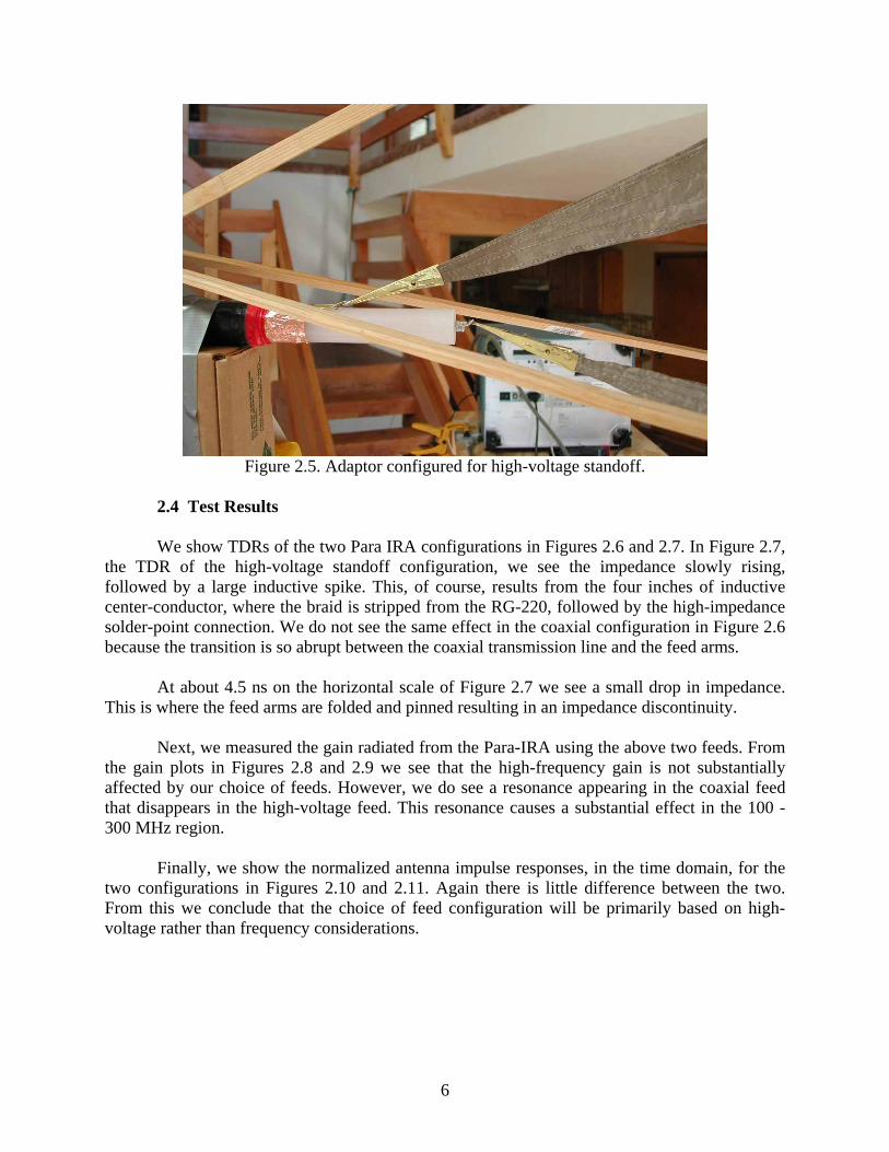
Figure 2.3. TDR and radiation setup to investigate the pulse generator to Para-IRA connection. Figure 2.4 shows the adaptor covered with copper tape to simulate the best possible high-frequency configuration. Figure 2.5 shows the adaptor configured for high voltage standoff. For the configuration of Figure 2.4 the excess material of the lower feed arms was folded and pinned to keep the feed arms taut.
Figure 2.4. Adaptor configured coaxially.
6
Figure 2.5. Adaptor configured for high-voltage standoff.
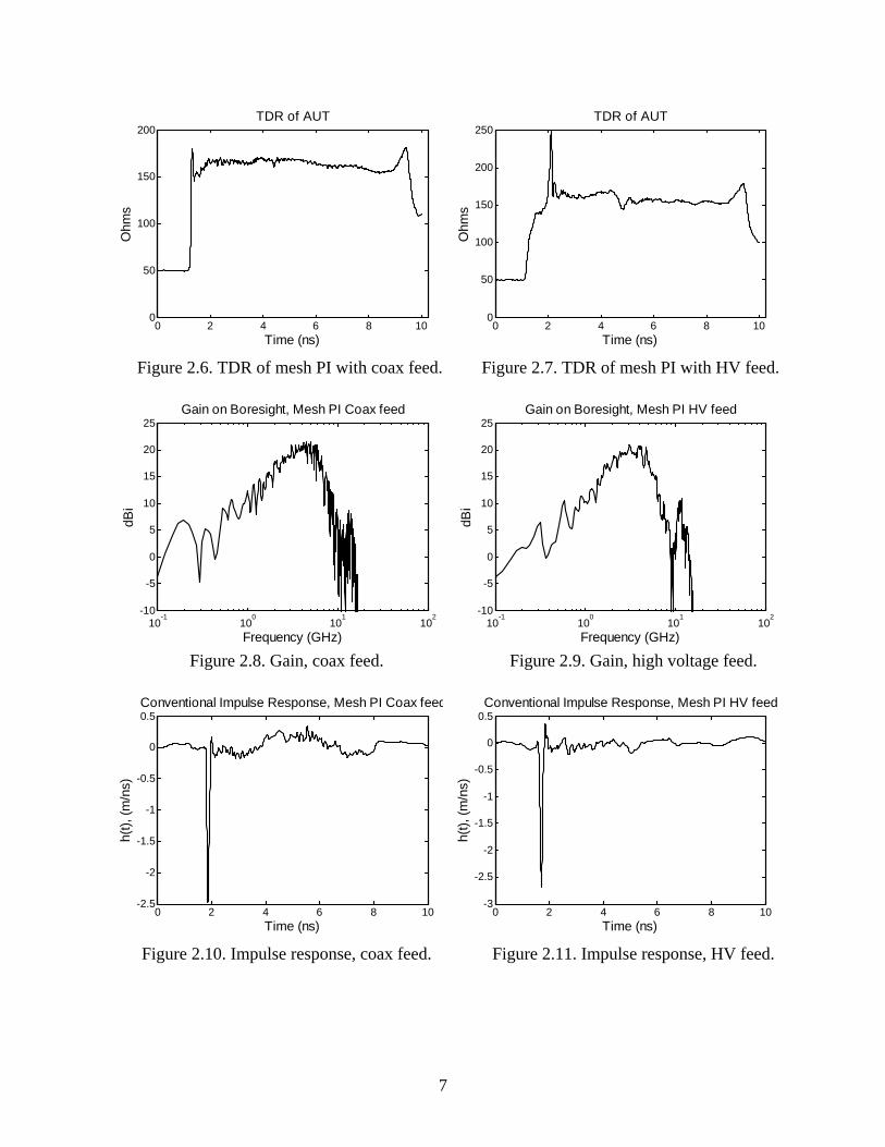
2.4 Test Results We show TDRs of the two Para IRA configurations in Figures 2.6 and 2.7. In Figure 2.7, the TDR of the high-voltage standoff configuration, we see the impedance slowly rising, followed by a large inductive spike. This, of course, results from the four inches of inductive center-conductor, where the braid is stripped from the RG-220, followed by the high-impedance solder-point connection. We do not see the same effect in the coaxial configuration in Figure 2.6 because the transition is so abrupt between the coaxial transmission line and the feed arms. At about 4.5 ns on the horizontal scale of Figure 2.7 we see a small drop in impedance. This is where the feed arms are folded and pinned resulting in an impedance discontinuity. Next, we measured the gain radiated from the Para-IRA using the above two feeds. From the gain plots in Figures 2.8 and 2.9 we see that the high-frequency gain is not substantially affected by our choice of feeds. However, we do see a resonance appearing in the coaxial feed that disappears in the high-voltage feed. This resonance causes a substantial effect in the 100 - 300 MHz region.
Finally, we show the normalized antenna impulse responses, in the time domain, for the two configurations in Figures 2.10 and 2.11. Again there is little difference between the two. From this we conclude that the choice of feed configuration will be primarily based on high-voltage rather than frequency considerations.
7
0 2 4 6 8 100
50
100
150
200TDR of AUT
Time (ns)
Ohm
s
0 2 4 6 8 100
50
100
150
200
250TDR of AUT
Time (ns)
Ohm
s
Figure 2.6. TDR of mesh PI with coax feed. Figure 2.7. TDR of mesh PI with HV feed.
10-1
100
101
102
-10
-5
0
5
10
15
20
25Gain on Boresight, Mesh PI Coax feed
Frequency (GHz)
dBi
10-1
100
101
102
-10
-5
0
5
10
15
20
25Gain on Boresight, Mesh PI HV feed
Frequency (GHz)
dBi
Figure 2.8. Gain, coax feed. Figure 2.9. Gain, high voltage feed.
0 2 4 6 8 10-2.5
-2
-1.5
-1
-0.5
0
0.5Conventional Impulse Response, Mesh PI Coax feed
Time (ns)
h(t),
(m/n
s)
0 2 4 6 8 10-3
-2.5
-2
-1.5
-1
-0.5
0
0.5Conventional Impulse Response, Mesh PI HV feed
Time (ns)
h(t),
(m/n
s)
Figure 2.10. Impulse response, coax feed. Figure 2.11. Impulse response, HV feed.

8
3. High Voltage Indoor Testing It was necessary to determine the characteristics of the ARC Technology Marx generator to ensure that we were applying an appropriate voltage to the Para-IRA. To make the required measurements accurately and without harming either personnel or instrumentation, we constructed a dummy load and a chamber for containing high voltages and radiated fields. We also developed a high-voltage fast-risetime derivative sensor. 3.1 Applied Physical Electronics High Voltage Pulser The 17-stage, ARC Technology Marx generator (manufactured by Applied Physical Electronics) is shown in Figure 3.1. It is approximately 1.1 meters (43 in.) long, 7.6 cm (3 in.) in diameter and weighs 6.4 kg (14 pounds). The end flanges are 11.4 cm (4.5 in.) in diameter. The output of the generator is an RG-220 coaxial cable 1.52 m (5 ft.) long, shown directly above the Marx. The output voltage is about 100 kV and the risetime is around 250 ps. Farr Research and ARC Technology jointly measured the Marx output voltage using the two different methods, a CVR, and a capacitively coupled pickoff probe built from an SMA panel-mount connector.
Figure 3.1. ARC Technology Marx generator.
3.2 Dummy Load We constructed a dummy load to test the Marx generator by terminating a section of RG-220 with a high-voltage 50-ohm 200-watt resistor. The RG-220 connects to the Marx output. We then used a Current-Viewing Resistor (CVR) to measure the Marx output. We found that energy from the dummy load terminating the Marx radiates directly into the recording oscilloscope, generating noise in our data. To solve that problem we surrounded the dummy load with a 30-gallon metal drum. The drum, when sealed with copper braid, effectively contains the fields generated in the wire-wound terminating resistor. 3.3 High-Voltage Containment Chamber We built a high-voltage, RF containment chamber from four, 85-gallon, steel drums. We cut up the drums and welded them back together to make a large steel cylinder with easily removable top and bottom. The chamber is lowered over prototype Para-IRA feed arms and transition section and then sealed. The ARC Technology pulser feeds the chamber from the bottom. The chamber is shown in Figure 3.2.

9
Figure 3.2. High voltage RF containment chamber.
3.4 Marx Testing 3.4.1 Current Viewing Resistor and SMA Pickoff We measured the output of the second, temporary, Marx using ARC Technology’s current viewing resistor (CVR) and the Farr Research SMA pickoff. The CVR sensor measures the current in the cable. In this design, the cable jacket is cut, a portion of the cable jacket is removed, and a number of resistors are inserted in parallel across the gap, thereby creating a low resistance in series with the outer cable jacket. The voltage across these resistors is proportional to the current in the coax. The SMA pickoff senses the derivative of the voltage in the coaxial cable. It is fabricated from a “sawed-off” SMA connector that is inserted through a small hole in the cable jacket. We show the SMA pickoff in Figure 3.3 and the SMA and CVR sensors as installed on the RG-220 cable in Figure 3.4.

10
Figure 3.3. Left: SMA connector modified as a sensor. Right: Sensor and hose clamp.
Figure 3.4. SMA sensor (left) and CVR sensor (right) installed onto the Marx output cable.
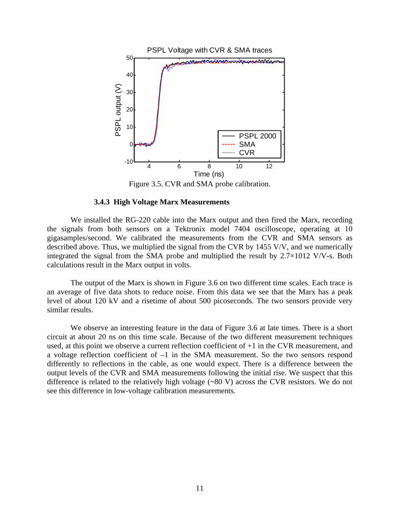
3.4.2 CVR and Pickoff Calibration We calibrated the CVR and SMA sensors as described in [3] by driving the cable with a known source, a Picosecond Pulse Laboratory model 2000D pulse generator. This has approximately a 48-volt output with a 300 ps risetime. We recorded the output from the CVR and SMA sensors on a Tektronix model TDS7404 oscilloscope operating at 10 gigasamples/second. We numerically integrated the SMA output and found a scalar that matches the integrated SMA data to the driving waveform. Similarly we found a scalar that matches the CVR data to the driving function. The scaled CVR and SMA data are shown in Figure 5.5, along with the output of the PSPL 2000D pulse generator. The calibration factor for the SMA is 2.7×10¹² V/V-s, and the calibration factor for the CVR is 1450 V/V.
11
4 6 8 10 12-10
0
10
20
30
40
50PSPL Voltage with CVR & SMA traces
Time (ns)
PS
PL
outp
ut (V
)
PSPL 2000SMACVR
Figure 3.5. CVR and SMA probe calibration.
3.4.3 High Voltage Marx Measurements We installed the RG-220 cable into the Marx output and then fired the Marx, recording the signals from both sensors on a Tektronix model 7404 oscilloscope, operating at 10 gigasamples/second. We calibrated the measurements from the CVR and SMA sensors as described above. Thus, we multiplied the signal from the CVR by 1455 V/V, and we numerically integrated the signal from the SMA probe and multiplied the result by 2.7×10¹² V/V-s. Both calculations result in the Marx output in volts. The output of the Marx is shown in Figure 3.6 on two different time scales. Each trace is an average of five data shots to reduce noise. From this data we see that the Marx has a peak level of about 120 kV and a risetime of about 500 picoseconds. The two sensors provide very similar results. We observe an interesting feature in the data of Figure 3.6 at late times. There is a short circuit at about 20 ns on this time scale. Because of the two different measurement techniques used, at this point we observe a current reflection coefficient of +1 in the CVR measurement, and a voltage reflection coefficient of –1 in the SMA measurement. So the two sensors respond differently to reflections in the cable, as one would expect. There is a difference between the output levels of the CVR and SMA measurements following the initial rise. We suspect that this difference is related to the relatively high voltage (~80 V) across the CVR resistors. We do not see this difference in low-voltage calibration measurements.

12
5 10 15 20 25-50
0
50
100
150Marx Output Voltage (CVR & SMA)
Time (ns)
Mar
x ou
tput
(kV
)
CVRSMA
9 9.5 10 10.5 11
0
50
100
150Marx Output Voltage (CVR & SMA)
Time (ns)
Mar
x ou
tput
(kV
)
CVRSMA
Figure 3.6. Marx output measured by CVR (solid) and SMA (dashed) probes.

13
4. Field within the Feed Arms 4.1 Feed Point Arcing When the feed point is not optimized we experience arcing. Figure 4.1 shows the integrated voltage output of the Prodyn model B-100 B-dot sensor and BIB1F balun combination (lower trace) and the Marx output voltage (upper trace). The integrated balun output voltage is scaled such that the two traces should overlay in the absence of arcing or reflections.
5 10 15 20
0
0.2
0.4
0.6
0.8
1
Overlay of integrated averaged raw data
Time (ns)
Nor
mal
ized
Mar
x O
utpu
t
Figure 4.1. Normalized Marx output (upper) and scaled B-100 sensor voltage (lower).
This data was taken at a reduced Marx charge, so the output level was approximately 100 kV. We are seeing feed-point arcing at about 40 kV Marx output level. Note that this was the initial setup with no precautions against arcing. Melting across the cable dielectric is visible where surface arcing occurred. 4.2 Feed Point Configurations We tested three feed point configurations for the Para-IRA by measuring the Marx output and the field generated within the feed arms. Our methodology was to start at a non-arcing configuration, regardless of its transmission-line or aerodynamic properties, then incrementally improve its characteristics. The first configuration is the baseline shown in Figure 4.2. The bare RG-220 dielectric is approximately 15.2 cm (6 in.) long. The second configuration (not pictured) tested is similar to baseline configuration except that feed arm separation was reduced to about 6.3 cm (2.5 in.). The third configuration tested is a shortened feed arm shown in Figure 7.3. Here the RG-220 dielectric is approximately 10.2 cm (4 in.) long.

14
Figure 4.2. Baseline feedpoint. Figure 4.3. Shortened feed point.
4.3 Test Data
We compare the Marx outputs and the magnetic field within the feed arms for the three configurations in Figures 4.4 through 4.9. During the shortened feed test, Figures 4.8 and 4.9, the Marx arced internally. This internal arcing is unrelated to the feed point length, but it does mean that the truncated Marx output (and possible internal Marx reflections) invalidates any data past the initial peak in these two figures. This data provides a basis for optimizing the feed point. Here we are looking at the initial peak only. Structure past the first peak is related to reflections and is not of interest. In Figure 4.8 the Marx is arcing internally, but we still see the first peak so the data remains valid for that time.
0 5 10 15 20 25
-40
-20
0
20
40
60
80
100
120
140Marx Output Voltage
Time (ns)
Mar
x ou
tput
(kV
)
0 5 10 15 20 250
500
1000
1500
2000
2500
3000
3500
4000H Within the Feedarms
Time (ns)
H (A
/m)
Figure 4.4. Marx output baseline configuration. Figure 4.5. H, baseline configuration.

15
0 5 10 15 20 25
-40
-20
0
20
40
60
80
100
120
140Marx Output Voltage
Time (ns)
Mar
x ou
tput
(kV
)
0 5 10 15 20 25-500
0
500
1000
1500
2000
2500
3000
3500
4000H Within the Feedarms
Time (ns)
H (A
/m)
Figure 4.6. Marx output reduced separation. Figure 4.7. H, reduced separation.
0 5 10 15 20 25
-40
-20
0
20
40
60
80
100
120
140Marx Output Voltage
Time (ns)
Mar
x ou
tput
(kV
)
0 5 10 15 20 25-500
0
500
1000
1500
2000
2500
3000
3500
4000H Within the Feedarms
Time (ns)
H (A
/m)
Figure 4.8. Marx output shortened feed point. Figure 4.9. H, shortened feed point. (Note that the Marx is arcing internally here.) 4.4 Conclusions The reduced separation and shortened feed point measurement define the minimum dimensions at which we can operate without feed point arcing. In other words, if the center conductor is not separated by at least this minimum distance from the outer-conductor feed arms, then arcing occurs at the feed point. Feed point arcing should not be confused with internal Marx arcing, which seems to be a function of the number of Marx firings accumulated before replacing the Marx liner (discussed above). If the feed length is shorter than the 10.2 cm (4 in.) length of the shortened feed, then arcing occurs at the feed point. The magnetic field measurement gives us a relative indication of feed point effectiveness between configurations. From these measurements, it is apparent that the reduced separation yields the highest field strength. In that configuration, we obtain over 2000 A/m initial peak versus about 1500 A/m initial peak in the baseline and shortened feed. From this we conclude that minimizing the separation is the best configuration for increasing the field radiating to the
16
reflector. An alternative feed was considered with a sharper arm divergence at the feed point to accommodate higher voltages. The shortened feed seems to have little effect on the radiated field compared to the baseline. Our conclusion is that the field launch is sensitive to the angular displacement, but less sensitive to the actual length of the feed.

17
5. Low-Voltage Testing 5.1 Low Voltage Test Fixture We tested a variety of feed points at low voltage in order to study their effect on the field launched between the feed arms. The low voltage test fixture is shown in Figure 5.1. The feed point configuration depends on the final design of high voltage Marx generator to feed arm transition device. With the low voltage fixture we were able to test various connections to optimize the transition. Several copper and silver colored tips for modifying the feed arms are visible on the plywood base.
Figure 5.1. Low voltage test fixture.
5.2 Low Voltage Feed Point Tests
We built several transition configurations, for testing with the low-voltage fixture, to find the best transition between the Marx generator and the Para-IRA feed arms. Figure 5.2 shows the basic configurations: a flush cut transition and zipper transitions of different lengths. Additionally we tested a very long transition to determine how the risetime will be affected. We found, not surprisingly, that increased high-voltage isolation is obtained with a long expanse of coaxial dielectric stripped of the outer conductor slows the risetime. Figure 5.3 shows photographs of the actual transitions.

18
Figure 5.2. Transition concepts: Flush cut, short zipper, long zipper.
Figure 5.3. Transition implementations: Flush cut, short zipper, long zipper, high voltage.
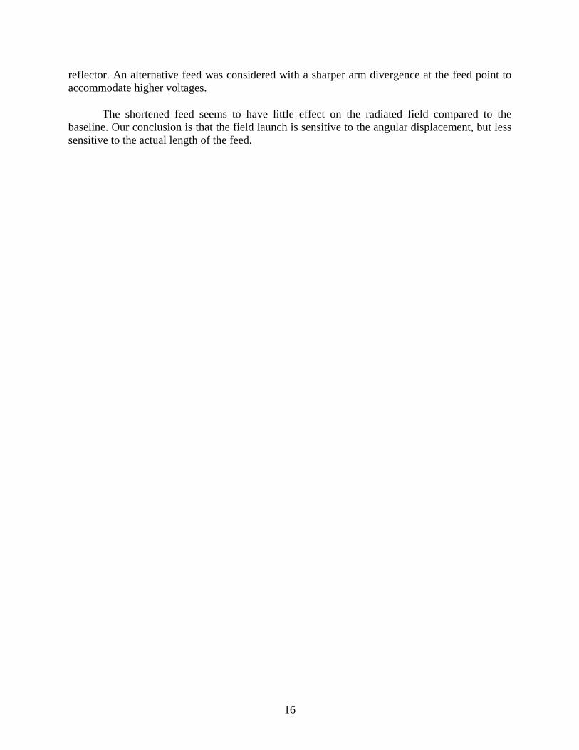
5.3 Feed Point Comparison and Selection We recorded the leading edge and peak field strength from each transition and we show the results in Figure 5.4. The flush transition shows the highest fidelity to the input step. The zipper and high-voltage transitions all show some overshoot. The 6.4-cm (2.5-in) zipper transition provides the best risetime and peak field strength, followed by the 3.8-cm (1.5-in) zipper. The long high-voltage transition has the slowest risetime and shows a pronounced ring. Ultimately for our high-voltage testing we chose the flush-cut transition to retain fidelity. An extended center conductor and dielectric 10.2 cm (4 in.) long was adequate to maintain the required high-voltage standoff.
19
0 0.2 0.4 0.6 0.8 1 1.2 1.4 -500
0
500
1000
1500
2000
2500
3000
3500
4000 Overlay of Flush and 1-1/2" & 2-1/2 Zipper
Time (ns)
Out
put (
V/m
)
Flush1 1/2" Zipper2 1/2" ZipperHigh Voltage Transition
Figure 5.4. Comparison between four feed configurations.
20
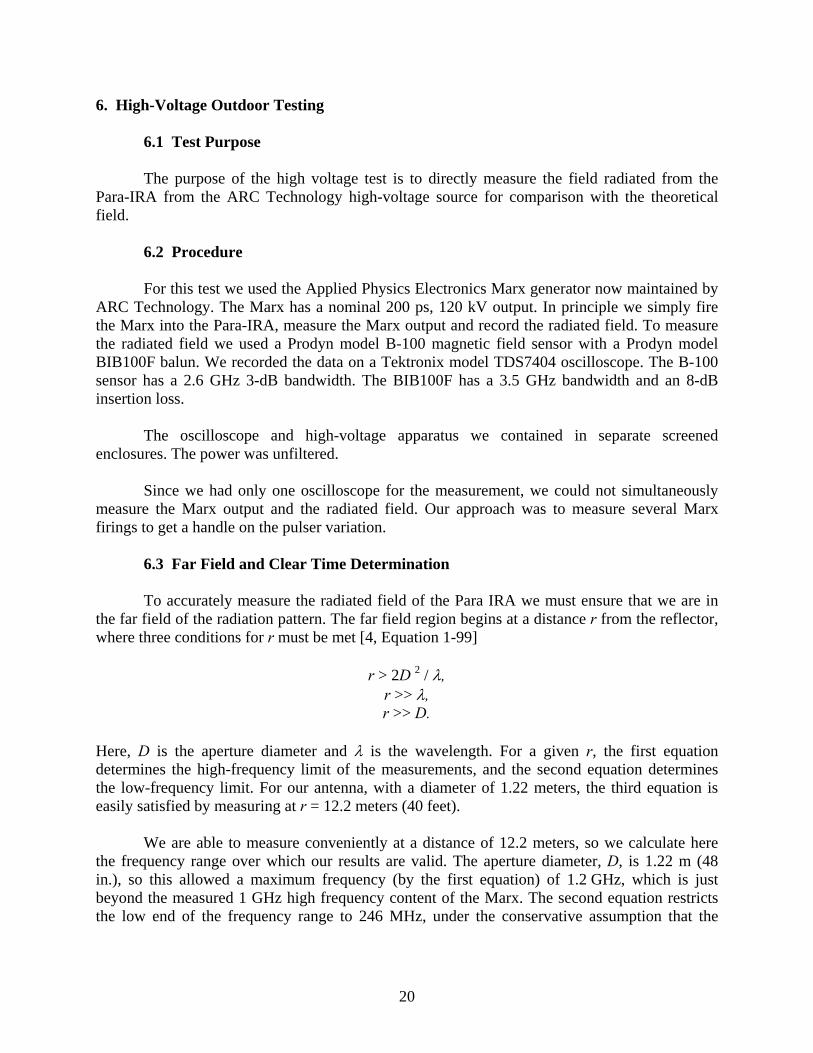
6. High-Voltage Outdoor Testing 6.1 Test Purpose The purpose of the high voltage test is to directly measure the field radiated from the Para-IRA from the ARC Technology high-voltage source for comparison with the theoretical field. 6.2 Procedure For this test we used the Applied Physics Electronics Marx generator now maintained by ARC Technology. The Marx has a nominal 200 ps, 120 kV output. In principle we simply fire the Marx into the Para-IRA, measure the Marx output and record the radiated field. To measure the radiated field we used a Prodyn model B-100 magnetic field sensor with a Prodyn model BIB100F balun. We recorded the data on a Tektronix model TDS7404 oscilloscope. The B-100 sensor has a 2.6 GHz 3-dB bandwidth. The BIB100F has a 3.5 GHz bandwidth and an 8-dB insertion loss. The oscilloscope and high-voltage apparatus we contained in separate screened enclosures. The power was unfiltered. Since we had only one oscilloscope for the measurement, we could not simultaneously measure the Marx output and the radiated field. Our approach was to measure several Marx firings to get a handle on the pulser variation. 6.3 Far Field and Clear Time Determination To accurately measure the radiated field of the Para IRA we must ensure that we are in the far field of the radiation pattern. The far field region begins at a distance r from the reflector, where three conditions for r must be met [4, Equation 1-99] r > 2D 2 / λ, r >> λ, r >> D. Here, D is the aperture diameter and λ is the wavelength. For a given r, the first equation determines the high-frequency limit of the measurements, and the second equation determines the low-frequency limit. For our antenna, with a diameter of 1.22 meters, the third equation is easily satisfied by measuring at r = 12.2 meters (40 feet). We are able to measure conveniently at a distance of 12.2 meters, so we calculate here the frequency range over which our results are valid. The aperture diameter, D, is 1.22 m (48 in.), so this allowed a maximum frequency (by the first equation) of 1.2 GHz, which is just beyond the measured 1 GHz high frequency content of the Marx. The second equation restricts the low end of the frequency range to 246 MHz, under the conservative assumption that the

21
symbol “>>” means “at least 10 times greater than.” So our measurements are valid over the frequency range, f, of
246 MHz < f < 1.2 GHz, and it could be argued that they are valid even lower with a less restrictive interpretation of the “>>” symbol. A related parameter of concern is clear time before ground reflections. Assume that both the Para-IRA reflector and the receiving antenna are the same height, h, above the ground. The path length difference between a direct ray and a ground-bounce ray for a separation of r = 12.2 meters and h = 3 meters (10 feet) will be about 1.4 meters or 4.7 nanoseconds. We will see approximately 4.7 ns of direct signal before the ground-reflected signal appears in the data. 6.4 Test Setup Figure 6.1 shows the instrumentation setup and physical layout. We show photographs of the test site in Figure 6.2. In this figure on the left of the top photograph we see the Para-IRA reflector on a tripod. Next is the Marx generator mounted on the wooden 2x4’s. The fiberglass ladder seen between the Marx and the B-dot sensor on the far tripod is only for setup and was removed during testing. The corner of a screen box can be seen in the lower left foreground. The bottom photograph shows detail of the reflector attached to the RG-220 cable coming from the Marx. We oriented the Para-IRA for a horizontal electric-field to minimize pickup on the vertical cables needed for charge lines and data cables.
A i r
TDS 7404
12.2 m(40 ft)
BounceGround TDS 7404
HV PSLV PS
Trig Gen
Marx
Screen Enclosure
MeshPara-IRA
B-100 SensorBIB-101F Balun
3.0 m(10 ft)
6.8 m
(22.4 ft)
Figure 6.1. Test instrumentation diagram.

22
Figure 6.2 Instrumentation layout (top) and detail of the Para-IRA mesh reflector (bottom).

23
6.5 Pulser Output Measurements We took ten shots on the Marx at 80% full charge (24 kV) to avoid damaging the Marx liner. The results are in Figure 6.3. The Marx output was processed by deconvolving the long data cable and pickoff impulse responses from the raw data. This data is an attempt to determine the pulser repeatability. We measured the risetime of the ten pulses to the first peak using the FWHM of the derivative. The average rise time of the ten pulses is 213 picoseconds compared to 200 ps nominal.
0 1 2 3 4 5-20
0
20
40
60
80
100
12010 Marx @ 80 percent charge
Time (ns)
Mar
x ou
t (kV
)
Figure 6.3. Overlay of 10 Marx pulses at 24 kV charge.
Next we went to full voltage (30 kV charge) on the Marx for three shots. Figure 6.4 is an overlay of the three shots. The repeatability seems to have suffered a bit at the higher levels. The output seems a bit too low also. We have 17.7 cm. (7 in.) of cable between the measurement pickoff and the feed point, corresponding to about 1.75 ns of clear time. The negative reflection occurring at about 2.5 ns on the horizontal scale is the reflection from the feed point. We measured the risetime time of the three pulses to the first peak using the FWHM of the derivative. The average rise time is 223 picoseconds and the average peak about 81 kV.
24
0 1 2 3 4 5-20
0
20
40
60
80
100
1203 Marx Outputs @ 100 percent charge
Time (ns)
Mar
x ou
t (kV
)
Figure 6.4. Overlay of three Marx pulses at 30 kV charge.
6.6 Boresight Measurements 6.6.1 Boresight Electric Field Predictions We provide here predictions of the field on boresight. The boresight electric field generated by the Para-IRA is determined from equations [5, equations 2.3 and 2.4] as:
dtdV
fcraE
grad π
τ2
=
where: Erad = radiated field, V/m τ = voltage transmission coefficient from the feed cable to the antenna, unitless (2) a = reflector radius, m (0.61 m) r = radial distance from the antenna, meters c = 3x10⁸ m/s fg = ratio of antenna impedance to free space impedance, unitless (200/377)ff V = source voltage For the Para-IRA, τ = 2, assuming a perfect balun design for a 50-ohm to 200-ohm impedance transition. The maximum source voltage divided by the risetime can approximate the derivative of the source voltage, dV/dt. Simplifying the above equation with the above values and approximations, we have
25
rrad t
Vr
E max-9 s101.7 ×
=
where: Vmax = maximum source voltage, volts tr = pulse risetime, seconds
We measured the Advanced Physical Electronics compact Marx pulser to have an initial peak voltage of 80 kV with a risetime of 220 ps. For this source fed into the antenna the resultant radiated field on boresight at 12.2 m is will be:
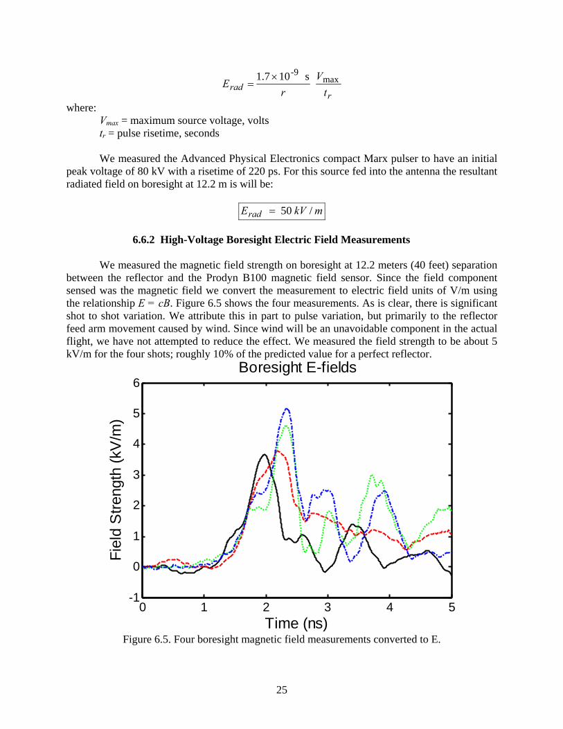
mkVErad /50= 6.6.2 High-Voltage Boresight Electric Field Measurements We measured the magnetic field strength on boresight at 12.2 meters (40 feet) separation between the reflector and the Prodyn B100 magnetic field sensor. Since the field component sensed was the magnetic field we convert the measurement to electric field units of V/m using the relationship E = cB. Figure 6.5 shows the four measurements. As is clear, there is significant shot to shot variation. We attribute this in part to pulse variation, but primarily to the reflector feed arm movement caused by wind. Since wind will be an unavoidable component in the actual flight, we have not attempted to reduce the effect. We measured the field strength to be about 5 kV/m for the four shots; roughly 10% of the predicted value for a perfect reflector.
0 1 2 3 4 5-1
0
1
2
3
4
5
6Boresight E-fields
Time (ns)
Fiel
d S
treng
th (k
V/m
)
Figure 6.5. Four boresight magnetic field measurements converted to E.

26
We attribute the lower-than-predicted field strength to several causes. First the predictive equation presumes a matching balun, which is not present in the test configuration, so there is a 50-ohm to 200 ohm mismatch at the feed point. Additionally, while we chose the best physical transition between the pulser and antenna to maintain pulse fidelity, to prevent arcing at the feed point we have a long, inductive feed presenting another impedance mismatch. Next, the wind was blowing during the test which deforms the feed arms significantly and unpredictably. 6.6.3 Low-Voltage Boresight Electric Field Measurements We tested this same reflector at an indoor range using a Kentech ASG1 pulse generator just before the high-voltage field testing. This generator has a 200-volt output with a 100-picosecond risetime. During this test the Para-IRA configuration was much more controlled. The feed arms were stretched and fixed in-place and wind was not a factor. For this low-voltage test we used the same sensor and balun as during the Marx test. The separation between antennas, r, for this indoor test was 6.8 meters, which is just short of the far-field measurement zone. This implies a small error inherent in this measurement. Calculating radiated electric field from the equation above predicts the electric-field strength to be 500 V/m. We measured 110 V/m for the field strength. We attribute the difference between the theoretical and measured values to the idealization of the equation including balun matching and the imperfections inherent in any physical implementation. The differences between the indoor and outdoor measurement are attributed primarily to wind effects distorting the reflector and feed arms. 6.7 Off Boresight Measurements Continuing now from the high-voltage outdoor measurements described in Section 6.6.2, we measured the field off-boresight in the E-plane. To do so, we moved the magnetic field sensor in five-degree steps to twenty degrees off boresight, keeping the 12.2 meter separation. We made two measurements at each off-boresight position. The off boresight fields are shown in Figure 6.6 through 6.9 again converted to electric field.
0 1 2 3 4 5-1
0
1
2
3
4
5
65-deg off boresight E-fields
Time (ns)
Fiel
d S
treng
th (k
V/m
)
0 1 2 3 4 5-1
0
1
2
3
4
5
610-deg off boresight E-fields
Time (ns)
Fiel
d S
treng
th (k
V/m
)
Figure 6.6. Two measurements at 5O. Figure 6.7. Two measurements at 10O.

27
0 1 2 3 4 5-1
0
1
2
3
4
5
615-deg off boresight E-fields
Time (ns)
Fiel
d S
treng
th (k
V/m
)
0 1 2 3 4 5-1
0
1
2
3
4
5
620-deg off boresight E-fields
Time (ns)
Fiel
d S
treng
th (k
V/m
)
Figure 6.8. Two measurements at 15O. Figure 6.9. Two cB measurements at 20O.
6.8 Comparison with Previous Test Results Finally, we compare the gain of the Para-IRA to that of the collapsible IRA. In Figure 6.10 we show the boresight realized gain of the Para-IRA [1, Figure 6.5]. Below it in Figure 6.11, we show the gain of the Farr Research commercial Collapsible Impulse Radiating Antenna, model CIRA-2 [6, Figure 4.5]. As the comparison shows, the gains are close, and the peak values for both are in the low-to-mid-20 dB range. With the exception of containing unresolved low frequency resonances, the mesh reflector compares well in gain and bandwidth to the commercial CIRA.
10-1
100
101
102
-10
-5
0
5
10
15
20
25
30Effective Gain on Boresight, Mesh PI term
Frequency (GHz)
dBi
Figure 6.10. The realized (effective) gain of the mesh prototype Para-IRA on boresight.

28
Figure 6.11. Gain of the CIRA on boresight, from [6, Figure 4.5]
6.9 Lessons Learned
• With the oscilloscope screen box opened, we had very large noise signal obscuring the data. Closing the screen box lid reduced the noise to acceptable levels. For quality testing we should have double walled screen boxes with filtered power.
• The Marx occasionally self-triggered, and this behavior became more frequent as the test
progressed. Consequently, some data are acquired on self-triggered Marx shots. Self-triggered shots are less repeatable than triggered shots.
• Low-level low-frequency ring is observed during magnetic field measurements. But it is
small enough to have little or no effect on the data, or data processing. • The present trigger system is somewhat unreliable. Towards the end of the test, the
trigger pulse may have been punching through the trigger cable, because the pulser became increasingly erratic and difficult to fire. If the Marx is to be used again on a test, we recommend either procuring a new trigger generator system that will be more immune to punch-through, or a Marx modification such that it triggers at a lower voltage.
• The present Marx generator is marginally reliable, because it would punch through after
five hundred to six hundred shots. This may be insufficient for its intended use.
• The magnetic field measurements obtained during outside testing with the fabric feed arms are more variable than we would like. Any wind causes the arms to flap. We

29
“cheated” by stapling narrow foam board strips to the arms to reduce the movement, but we still had significant flapping, which resulted in large field variations.
• The magnetic field variation may be due to pulser variation or feed arm flapping. We will
need two oscilloscopes simultaneously acquiring data to remove the pulser variation to isolate the problem.
30
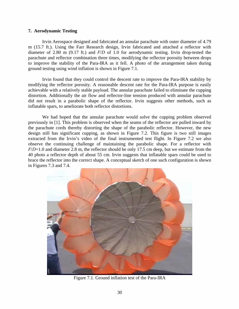
7. Aerodynamic Testing Irvin Aerospace designed and fabricated an annular parachute with outer diameter of 4.79 m (15.7 ft.). Using the Farr Research design, Irvin fabricated and attached a reflector with diameter of 2.80 m (9.17 ft.) and F/D of 1.0 for aerodynamic testing. Irvin drop-tested the parachute and reflector combination three times, modifying the reflector porosity between drops to improve the stability of the Para-IRA as it fell. A photo of the arrangement taken during ground testing using wind inflation is shown in Figure 7.1. Irvin found that they could control the descent rate to improve the Para-IRA stability by modifying the reflector porosity. A reasonable descent rate for the Para-IRA purpose is easily achievable with a relatively stable payload. The annular parachute failed to eliminate the cupping distortion. Additionally the air flow and reflector-line tension produced with annular parachute did not result in a parabolic shape of the reflector. Irvin suggests other methods, such as inflatable spars, to ameliorate both reflector distortions. We had hoped that the annular parachute would solve the cupping problem observed previously in [1]. This problem is observed when the seams of the reflector are pulled inward by the parachute cords thereby distorting the shape of the parabolic reflector. However, the new design still has significant cupping, as shown in Figure 7.2. This figure is two still images extracted from the Irvin’s video of the final instrumented test flight. In Figure 7.2 we also observe the continuing challenge of maintaining the parabolic shape. For a reflector with F/D=1.0 and diameter 2.8 m, the reflector should be only 17.5 cm deep, but we estimate from the 40 photo a reflector depth of about 55 cm. Irvin suggests that inflatable spars could be used to brace the reflector into the correct shape. A conceptual sketch of one such configuration is shown in Figures 7.3 and 7.4.
Figure 7.1. Ground inflation test of the Para-IRA

31
Figure 7.2. Two profiles of the Para-IRA during the final test flight.
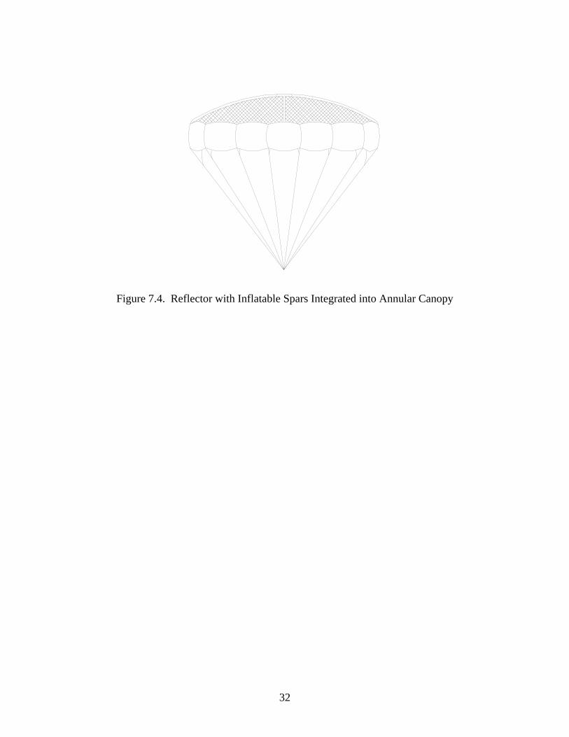
Figure 7.3 shows one variant of the Reflector with inflatable spars alone, while Figure 7.4 shows the Reflector with inflatable spars integrated into an Annular Canopy. It may be useful to investigate some variation of this in the future, in order to achieve a reflector that is more smooth.
Figure 7.3. Reflector with Inflatable Spars, Side View (Top) and Top View (Bottom)
Inflatable Spars
Metallized Mesh
Inflatable Spars
Mesh (Typ. 4 Places)
32
Figure 7.4. Reflector with Inflatable Spars Integrated into Annular Canopy
33
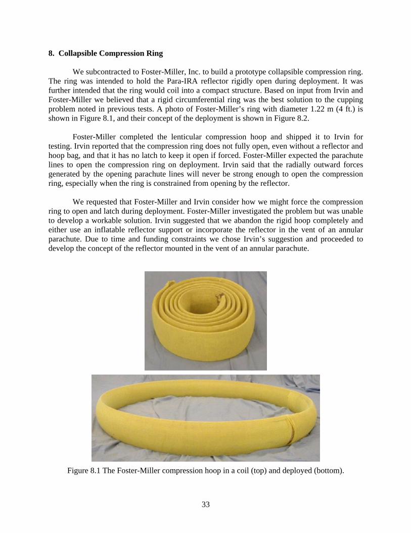
8. Collapsible Compression Ring We subcontracted to Foster-Miller, Inc. to build a prototype collapsible compression ring. The ring was intended to hold the Para-IRA reflector rigidly open during deployment. It was further intended that the ring would coil into a compact structure. Based on input from Irvin and Foster-Miller we believed that a rigid circumferential ring was the best solution to the cupping problem noted in previous tests. A photo of Foster-Miller’s ring with diameter 1.22 m (4 ft.) is shown in Figure 8.1, and their concept of the deployment is shown in Figure 8.2. Foster-Miller completed the lenticular compression hoop and shipped it to Irvin for testing. Irvin reported that the compression ring does not fully open, even without a reflector and hoop bag, and that it has no latch to keep it open if forced. Foster-Miller expected the parachute lines to open the compression ring on deployment. Irvin said that the radially outward forces generated by the opening parachute lines will never be strong enough to open the compression ring, especially when the ring is constrained from opening by the reflector. We requested that Foster-Miller and Irvin consider how we might force the compression ring to open and latch during deployment. Foster-Miller investigated the problem but was unable to develop a workable solution. Irvin suggested that we abandon the rigid hoop completely and either use an inflatable reflector support or incorporate the reflector in the vent of an annular parachute. Due to time and funding constraints we chose Irvin’s suggestion and proceeded to develop the concept of the reflector mounted in the vent of an annular parachute.
Figure 8.1 The Foster-Miller compression hoop in a coil (top) and deployed (bottom).
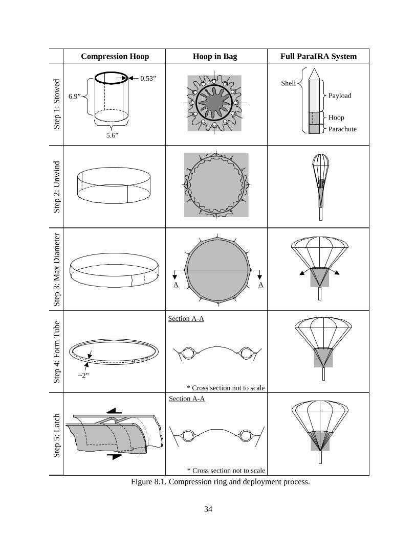
34
6.9”
5.6”
0.53”
Compression Hoop Hoop in Bag Full ParaIRA SystemSt
ep 1
: Sto
wed
St
ep 2
: Unw
ind
St
ep 3
: Max
Dia
met
er
Step
4: F
orm
Tub
eSt
ep 5
: Lat
ch
Payload
Hoop Parachute
Shell
~2”
* Cross section not to scale
* Cross section not to scale
A A
Section A-A
Section A-A
Figure 8.1. Compression ring and deployment process.
35
9. Conclusions We have completed a series of tests to study the properties of Parachute Impulse Radiating Antennas, or Para-IRAs at both low and high voltages. We tested several configurations for driving the Para-IRA with the Marx generator. We obtained the best pulse shape with the shortest feed at the narrowest angle, with a flush-cut outer-conductor on the pulser cable. However, this configuration is a poor choice for high-voltage standoff. For this reason, we ultimately fed the Para-IRA with a 10.2 cm (4 in.) length of cable stub, from which the outer conductor was removed. We experimented with the ARC Technology Marx generator. We improved its reliability by replacing the internal acrylic liner with a UHMW polyethylene liner, in order to increase the number of shots before punch-through. Reliable triggering remains a challenge, and we obtained peak voltages of around 120 kV. This is somewhat less that we expected from a 17-stage Marx that is charged to 30 kV. We measured the radiated field of the Para-IRA when driven at full voltage, and we found the field strength is lower than originally predicted. A number of effects could have lowered the radiated field, including deformation of the antenna by the wind, physically large components, and a pulse shape that is less than ideal. The high-voltage Para-IRA radiated field levels were about ten percent of the predicted values. This value is down from the indoor testing which yielded an empirical field strength of about twenty percent of the predicted value. To maintain a smooth surface on the reflector, we tried mounting it to a parachute with an annular design. However, during static ground tests and airborne drop tests we still observed significant cupping of the reflector near the attachment points. The annular parachute and reflector combination remain an interesting design because its descent rate is adjustable, which provides stability during descent. But the annular design of the parachute did not eliminate gore cupping in the reflector. In another attempt to address the cupping problem, we worked with Foster-Miller, Inc. to develop a rigid compression ring to hold the circumference round. However, the compression ring did not open with sufficient force, so it could not be locked into the open position. We found no remedy for this problem, so that approach will likely be abandoned. To address the cupping problem on the reflector, one option is to investigate an inflatable spar system as described in Section 7. This should maintain the rigidity of the circumference and the parabolic shape of the reflector and support system. While this would increase the complexity of the Para-IRA, it may well be necessary. The stability of descent of our Para-IRA also remains a challenge, because we observed oscillations in the pointing angle of the antenna of 10-20°. This may be acceptable in a some systems that require broad coverage, but it may be a concern if a more precise aim is required. The instability arises because the high-mass pulser is located too close to the parachute. In our tests, we placed the pulser near the focus of the reflector, with F/D=1. However, for maximum
36
stability, the center of mass is normally positioned below the canopy a distance of 2-3 times the diameter of the canopy. We cannot increase the F/D ratio of the reflector beyond unity without degrading the performance of the antenna. We can try two approaches for lowering the center of mass of the load on the parachute. First, we could add a weight well below the pulser. This weight might be a battery, or it might be a dead weight. Note that the use of a dead weight will make it more difficult to maintain size and weight constraints of the system. Alternatively, we could position the pulser well below the focus of the reflector, and feed the antenna with a long cable. In our version of the Para-IRA, we used RG-220 cable to feed the antenna. This cable is not easily bent or coiled, so a long length of it cannot be easily fitted into a small package. Thus, a smaller cable may be needed, which would limit the driving voltage. Acknowledgement We are pleased to acknowledge the support of U.S. Army / Space and Missile Defense Command for funding this work. References 1. L. M. Atchley, E. G. Farr, J. S. Tyo, and Larry L. Altgilbers, Development and Testing of a
Parachute Deployable Impulse Radiating Antenna, Sensor and Simulation Note 465, March2002.
2. L. M. Atchley, E. G. Farr, and L. L. Altgilbers, Experimental Studies of Scale-Model and
Full-Scale IRAs Mounted on Parachutes, Sensor and Simulation Note 478, July 2003. 3. E. G. Farr, L. M. Atchley, D. E. Ellibee, and L. L. Altgilbers, A Comparison of Two Sensors
Used to Measure High-Voltage, Fast-Risetime Signals in Coaxial Cable, Measurement Note 58, March 2004.
4. W. L. Stutzman and G. A. Thiele, Antenna Theory and Design, 2nd edition, Wiley, 1998. 5. E. G. Farr, C. E. Baum, Time Domain Characterization of Antennas with TEM Feeds, Sensor
and Simulation Note 426, October 1998. 6. L. H. Bowen, E. G. Farr, and W. D. Prather, An Improved Collapsible Impulse Radiating
Antenna, Sensor and Simulation Note 444, April 2000.