Send in the Clones?

Hedge Fund Replication Using Futures Contracts

Nicolas P.B. Bollen†

Gregg S. Fisher

This version: July 3, 2012

Abstract

Replication products strive to offer investors some of the benefits of hedge funds while avoiding their high fees, illiquidity, and opacity. We test whether a replication algorithm can deliver the diversification and high Sharpe ratio that investors seek. Our procedure constructs monthly clone returns out-of-sample using fully collateralized futures positions held for one-month, with position sizes determined using rolling window regressions. Clone returns have high correlation with their hedge fund targets, indicating replication is possible. Clones also have high correlation with a buy-and-hold investment in stocks, however, and neither the targets nor their clones demonstrate successful time variation in factor loadings.

†Bollen is the E. Bronson Ingram Professor of Finance, Owen Graduate School of Management, Vanderbilt University. Email nick.bollen@owen.vanderbilt.edu. Phone (615) 343-5029. Fisher is President and Chief Investment Officer of Gerstein Fisher. Thanks to Spencer Hezzelwood for excellent research assistance. Bob Whaley, Jacob Sagi, and seminar participants at Vanderbilt University provided useful comments.

1  

Send in the Clones? Hedge Fund Replication Using Futures Contracts

1. Introduction

The hedge fund industry recovered quickly from the contraction experienced in the post-financial

crisis period, with aggregate assets under management exceeding $2 trillion during Q1 2012.1

Several issues continue to keep many investors on the sidelines, however, including a spate of

insider-trading scandals, opaque holdings, and high fees. In an effort to cater to the demand for

an alternative investment that offers some of the benefits of hedge funds while avoiding these

problems, a number of financial institutions have developed a new set of products using

relatively liquid, transparent, and low-cost strategies. The goal of this article is to determine the

performance and appropriate use of these hedge fund clones.

Most hedge fund replication products attempt to mimic the future time series properties

of a target fund or fund index by constructing a portfolio of investable factors that matches the

target’s historical returns as closely as possible.2 The factors represent investments in asset

classes such as equities, fixed income, and commodities. The dynamic nature of the target’s

actual unobserved trading strategy requires that the composition of the clone portfolio changes

over time. To achieve this, hedge fund replication is an iterative process, in which the target’s

exposures to the factors are re-estimated periodically and the allocation weights of the clone are

adjusted accordingly.

To understand what clones can and cannot capture, it is useful to consider the classic

decomposition of managerial skill into security selection and market timing. Because the target’s

actual positions are unknown, it is impossible to try to capture security selection. This limitation

is reflected in the generic building blocks of replication products: liquid securities such as futures

contracts or ETFs. What factor-based replication can offer, however, is a procedure for

attempting to match the factor timing activity of a target. As hedge fund managers trade, the

correlation between fund returns and those of the investable factors change. These changes are

then translated by the replication procedure into new allocation weights. If managers have timing

skill, then the clone will feature higher allocation to a factor during periods of high returns. To

                                                            1 HFR Market Microstructure HF Industry Report – Q1 2012. 2 See, for example, descriptions of IndexIQ’s offerings at www.indexiq.com and a series of exchange traded notes designed by Credit Suisse at https://notes.credit-suisse.com/csfbnoteslogin/etn/csetns.asp.

2  

test the effectiveness of factor-based replication, therefore, we employ several tests of market

timing ability.

We choose the Dow Jones Credit Suisse hedge fund indexes as our target investments.

These indexes are asset-weighted portfolios of hedge funds selected on the basis of capacity and

other operational risk requirements. We choose to replicate hedge fund indexes as opposed to

individual funds since University endowments, pension funds, and other institutional investors

typically invest in portfolios of funds.3 To create the clones, we use a parsimonious set of five

liquid futures contracts to permit low-cost exposure to major asset classes. The clone procedure

is based around a series of rolling window regressions to estimate the time varying exposure of

the hedge fund indexes to the asset classes. Each regression yields a set of allocation weights

which are then used to construct a clone portfolio that is held for one-month out-of-sample. We

vary implementation details, such as the estimation window length, to determine their impact on

clone performance.

Our methodology is similar to that of Hasanhodzic and Lo (2007), who estimate linear

factor models using returns of individual hedge funds for the purpose of constructing replicating

portfolios. We make three contributions. First, the set of factors used by Hasanhodzic and Lo are

not all investable, including, for example, the Goldman Sachs Commodity Index and the spread

between the Lehman BAA Corporate Bond Index and the Lehman Treasury Index. In contrast,

all of our factors are returns on liquid futures contracts. Second, their sample period ends in

2005, prior to the global financial crisis. Our sample extends an additional six years, allowing us

to comment on clone performance directly before and after the turmoil that has defined

investments ever since. Third, and perhaps most important, we argue that the only way clones

can add value is by capturing the factor timing activity of the target, thereby motivating our

analysis of the market timing ability of the clones.

The rest of the paper proceeds as follows. Section 2 reviews relevant prior literature on

hedge fund replication, factor models, and market timing. Section 3 provides details about the

data used in the study and presents some of the empirical methods. The cloning procedure and

empirical results are described in Section 4. Section 5 offers a brief summary with concluding

remarks.                                                             3 In addition, Bollen (2012) argues that the ability of factor models to explain individual fund returns is quite limited.

3  

2. Prior Literature

2.1. Competing Replication Procedures

There are two main approaches to replicating hedge funds. Factor-based replication takes

positions in liquid instruments to match the target fund’s exposures to a number of risk factors.

Factor-based clones are typically assessed by their ability to mimic the returns of the target fund

out-of-sample. Distribution-based replication uses complex trading strategies to match the

historical return distribution of the target fund. Distribution-based clones are typically assessed

by their ability to mimic the distribution of the target fund out-of-sample, either the

unconditional distribution, as in Amin and Kat (2003), or the bivariate distribution of the target

fund return and the return of some other asset such as a stock market index, as in Kat and Palaro

(2005).

We focus on factor-based replication for three reasons. First, using a distribution as the

basis for replication requires a relatively long time period to establish the target distribution ex-

ante using historical returns, estimate the resulting clone’s distribution ex-post, and asses its

similarity to that of the target. Using the necessarily long time series is problematic since hedge

fund return distributions are highly transitory given the freedom with which managers can

change investment strategies and leverage ratios. Furthermore, Amenc et al. (2008) show that

distribution-based clones achieve out-of-sample success only over long assessment periods of at

least six years. It is unlikely that investors would have the patience to wait six years before

evaluating investment performance.

Second, the distribution-based clones rely on relatively sophisticated mathematical

techniques, which can be traced to Dybvig (1988), to create a high-frequency trading system. For

many investors the appeal of clones is their transparency. While the distribution-based clone’s

trade engine can be explicitly defined and shared with investors, for many it will remain a black

box. Third, by construction, distribution-based clones do not attempt to match the month-by-

month returns of a target fund, and so have difficulty matching the conditional distribution of

target returns. The exception to this is the bivariate distribution target of Kat and Palaro (2005),

but in their out-of-sample tests they fail to match target returns during volatile periods.

4  

2.2. Factor Models and Factor-Based Clones

The mechanics of factor-based replication can be attributed to Sharpe (1992), who infers

asset allocation choices using a linear factor model to measure the relation between the returns of

an investment vehicle and those of standard asset classes. Sharpe then applies the model to a

sample of open-end mutual funds and shows how estimates of factor loadings correspond to the

expected asset mix of each fund given their stated investment style. As discussed by Fung and

Hsieh (2001), the combination of a linear structure and buy-and-hold factors is inappropriate for

analysis of hedge funds given the non-linear relation between hedge fund returns and those of

standard assets. Non-linearities can be generated by dynamic exposure via relatively high

frequency trading and by positions in securities with option-like payoffs such as credit default

swaps. Linear factor models can capture dynamic exposure to an underlying asset or strategy if

factor loadings are allowed to change over time. This is the approach implicit in our use of

rolling estimation windows when establishing clone portfolios, as described below.

Like Hasanhodzic and Lo (2007), Amenc et al. (2008) test the out-of-sample performance

of factor-based clones. When comparing one-month out-of-sample clone returns to their target

returns they find correlations typically below 0.50 and low regression R-squared. They conclude

that linear-based clones do not work well, and argue that a major weakness is the inability of

linear factor models to capture the time varying exposure of hedge funds to underlying factors.

Amenc et al. conclude that non-linear factor models may be the solution. Amenc et al. (2010)

study whether non-linear factor models can improve the performance of factor-based clones by

estimating a regime-switching model as well as a model of stochastic exposures using a Kalman

filter. Perhaps not surprisingly, the in-sample fit of these models with time varying factor

exposures is superior to that of fixed exposures. More importantly, the out-of-sample

performance is no better and in many cases is inferior to the simpler model, suggesting a risk of

over-fitting.

In this paper, we employ rolling estimation windows to allow for time varying exposures

to underlying asset classes. Though somewhat crude, the results in Amenc et al. (2010) illustrate

that more sophisticated techniques are plagued by over-fitting and poor out-of-sample

performance. In addition, a natural consequence of a rolling window is that factor exposures can

5  

evolve smoothly over time, depending on the length of the estimation window, resulting in a

relatively low rate of portfolio turnover in the clone.

2.3. Estimating Market Timing Ability in Factor Models

As described in Section 1, an appropriate goal for factor-based replication is to capture

the market timing ability of a target. There are two ways to estimate market timing ability in the

context of a factor model.

First, one can estimate exposures to factors that are constructed to reflect the returns of

active market timing strategies. Fung and Hsieh (2001), for example, develop a family of trend-

following factors to capture dynamic exposures of funds to various asset classes including

equities, bonds, currencies, and commodities. These factors are constructed from portfolios of

options in order to replicate a look-back straddle, which in turn generates payoffs equivalent to a

successful market timer. While these factors have been widely adopted in hedge fund research to

characterize the risk and return profile of hedge funds, they are problematic in the context of

replication because they are not readily investable. We limit the set of factors to futures contracts

in order to construct a low-cost, liquid investment vehicle.

Second, one can use a model that allows for exposures to standard asset classes that vary

conditional on the magnitude of asset returns. Treynor and Mazuy (1966), for example, specify a

quadratic relation between the returns of a fund and those of the market, allowing for a larger

exposure during higher market returns. Similarly, Henriksson and Merton (1981) use a piece-

wise linear relation between the returns of a fund and those of the market, allowing for different

levels of exposure when the market return is above or below a certain level. We use both of these

factor models to measure the timing ability of the hedge fund indexes and their clones.

To set expectations, note that prior literature provides limited evidence of market timing

ability in hedge funds. Chen (2007) and Chen and Liang (2007) find some evidence of market

timing in small subsets of funds. Chen and Liang study the timing ability in a sample of 221

funds that are either explicitly categorized as belonging in a market timing style or describe

themselves as such in their prospectus. They find that these funds feature, both individually and

collectively, some ability to vary equity market exposure in advance of market moves. Chen

6  

finds no evidence of equity market timing ability in a broader sample of funds, but some

evidence of the ability to time bond and currency in global macro and managed futures funds.

Griffin and Xu (2009) examine timing ability using equity holdings of hedge funds observed

from quarterly SEC Form 13F filings. They find no evidence that hedge fund managers can

rotate capital among different styles in advance of high returns.

3. Data and Empirical Methods

3.1. Hedge Fund Indexes

Monthly returns of 10 Dow Jones Credit Suisse indexes are used as our targets.4 The set

includes a broad index as well as nine strategy-focused sub-indexes. The indexes are constructed

by Credit Suisse Hedge Index LLC using an asset-weighted average return of hedge funds in the

Credit Suisse Hedge Fund Database, formerly known as the Credit Suisse/Tremont Hedge Fund

Database. To be included in an index, a fund must meet a number of requirements, including

assets under management of at least $50 million, current audited financial statements, and a

minimum 12-month track record. To avoid a censoring bias, liquidating funds are kept in an

index until the liquidation is complete, thereby generating a more accurate reflection of hedge

fund performance.

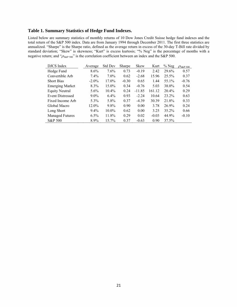
Summary statistics for the 10 indexes, as well as the total return of the S&P 500 for

comparison, are listed in Table 1 using the full sample from January 1994 through December

2011. The broad Hedge Fund Index handily outperforms the S&P 500 over this period, with

comparable average return but only half the volatility, resulting in an annualized Sharpe ratio of

0.73 for the Hedge Fund Index versus 0.37 for the S&P 500. Note, however, that the correlation

between the two is a relatively high 0.57. The other indexes feature substantial variation in

performance, four of which generate lower Sharpe ratios than the S&P 500. Annualized average

returns range from –2.0% for the Short Bias Index to 12.0% for the Global Macro Index.

Annualized standard deviations range from 5.8% for the Fixed Income Arbitrage Index to 17.0%

for the Short Bias Index.

                                                            4 Data downloaded from www.hedgeindex.com.

7  

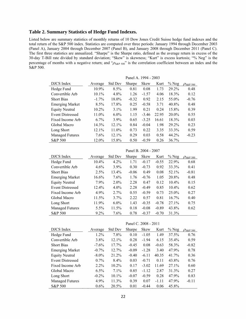
Table 2 shows the same statistics computed over three subsets of the data: 1994 – 2003,

2004 – 2007, and 2008 – 2011. Dramatic variation exists across the subsets, as one would expect

given the impact of the financial crisis in the most recent period. The Hedge Fund Index, for

example, features Sharpe ratios of 0.81, 1.71, and 0.10 over the three periods, respectively. The

non-stationarity in index return distributions displayed here illustrates the difficulty in replication

procedures that focus on matching the return distribution of a target. Importantly, correlations

between the hedge fund indexes and the S&P 500 have general increased over time. The Hedge

Fund Index has a correlation of 0.48 in the first period, rising to 0.68 in the second and 0.76 in

the most recent period. This result suggests that our ability to match hedge fund returns may

improve over time as correlations with systematic risk factors increase.

3.2. Replication Building Blocks

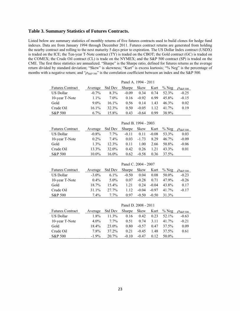
We use positions in five futures contracts to construct clones for each hedge fund index. 

Futures contract returns are generated from holding the nearby contract and rolling to the next

maturity 5 days prior to expiration. The US Dollar Index contract (USDX) is traded on the ICE;

the Ten-year T-Note contract (TY) is traded on the CBOT; the Gold contract (GC) is traded on

the COMEX; the Crude Oil contract (CL) is trade on the NYMEX; and the S&P 500 contract

(SP) is traded on the CME. Summary statistics over the full sample, and three subsets, are listed

in Table 3. Over the full sample, Crude Oil has the highest average return and standard deviation,

16.1% and 32.3%, respectively. Gold delivers a slightly higher Sharpe ratio than Crude Oil, 0.56

as compared to 0.50. Correlations between each contract and the S&P 500 are generally low, and

in many cases negative. The US Dollar contract, for example, features a correlation of ‒0.25 over

the full sample and ‒0.63 over the most recent period, as dollar-denominated assets were in high

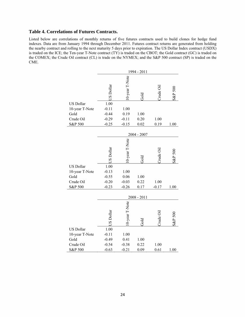
demand during the crisis. Correlations between each pair of contracts are listed in Table 4. The

US Dollar and Ten-year T-Note contracts are negatively related to all other assets, with the

exception of the Ten-year T-Note and Gold pair. These two assets feature a correlation of 0.41 in

the most recent period as investors world-wide fled to safe assets.

One might question our choice of building blocks given the large number of potential

candidates and the standard sets of factors used in hedge fund research. The Fung and Hsieh

(2004) seven-factor model, for example, is the most widely adopted set of factors used in

8  

academic studies of hedge fund risk. We have two concerns which lead us to the five factors

described above. First, as mentioned in Section 2, some of the Fung and Hsieh factors are not

readily investable. In particular, implementing the trend-following strategies introduced in Fung

and Hsieh (2001) would require a great deal of trading in derivative securities. While they may

be useful for describing the types of assets and strategies hedge funds use, in the context of this

replication study they are not as relevant. Second, though we are using an out-of-sample

procedure for assessing the performance of the clones, searching over a potentially large set of

factors raises the specter of data-mining. A large enough set almost guarantees we could

construct clones that appear to perform well, but then we lose the benefit of an out-of-sample

assessment.

Given investor demand for a product that can help diversify holdings of standard asset

classes, one might also question our choice of the S&P 500 and Ten-year T-Note contracts.

There are two reasons why we include them. First, recall our goal is to replicate the time series of

returns of a hedge fund or hedge fund index. If the match between the target and the clone

returns is tight, then the clone will inherit the salient features of the target, including its

correlation with other assets. Whether the S&P 500 and Ten-year T-Note contracts help match

the target is an empirical question which our analysis will answer. Second, our replication

procedure allows for negative and time varying factor exposures, so even a clone consisting

solely of these two contracts could deliver low correlation with a buy-and-hold investment in

stocks and bonds.

3.3. Clone construction

Clones are constructed by estimating coefficients of a linear factor model each month.

Coefficients are used as position sizes for the five futures contracts. Positions are entered with a

one month delay to realistically reflect the actions of the replication methodology in real time as

described below.

To construct the clone return for month t, we use data through month t – 2. So, for

example, the clone return for January would be based on a regression using data through the

prior November. This represents a one month lag between the end of an index reporting period

and establishing the futures positions for replicating the index. The index performance is

9  

typically available on the 15th of a given month, so the procedure in effect allows for a two-week

period between obtaining the most recent index return and establishing the futures positions. The

clone return for January, for example, would be based on index returns through November,

which would be available in mid-December. The requisite futures positions would then be

entered at the end of December. See Figure 1 for a timeline that illustrates the sequence of

events.

A five-factor regression run on date t – 2 and using T observations is expressed as:

(1) 5

, , , ,1

1, 2i j i k k j i jk

r r j t T t

where ri is the excess return of the index and rk is the return of one of five factors. This

regression differs from standard factor models because, following Hasanhodzic and Lo (2007),

we have suppressed the intercept, which is typically labeled alpha. Alpha is a primary measure of

fund performance, and can be interpreted as the capturing the security selection ability of a

manager. Note in our context, however, that it is impossible to replicate alpha; indeed, in the

language of regression, the intercept is the averaged unexplained return. By omitting the

intercept we are forcing the factors to play a larger role fitting the target’s returns. A chief

concern of “regression through the origin” is that estimates of will be biased. We will assess

this by focusing on out-of-sample tests of the clone’s ability to fit the target return.

We conduct the exercise with four different estimation periods of T = 12, 24, 36, and 48

months. Since this is a regression of excess index returns on the realizable returns of futures

positions, the coefficients can be interpreted as percentage allocation weights of clone capital

to notional futures positions. Given the coefficient estimates, computing the clone return rc for

date t begins with the date t fitted value of the regression:

(2) 5

, , ,1

c t i k k tk

r r

We assume that the futures positions are “fully collateralized” meaning that for every dollar of

notional exposure, positive or negative, a dollar of cash is set aside in an interest bearing

account. This assumption makes the coefficients easy to interpret – a coefficient of 1.0 means

100% of the clone assets are invested in the associated contract. We assume that cash earns the

10  

one-month LIBOR rate. In addition, we sum the absolute values of the from the regressions,

where a negative simply indicates a short position in the futures contract. The sum of the

absolute values indicates the percentage of the clone’s capital that is deployed as notional futures

exposure. If this sum is less than 100%, we assume the remainder of a clone’s capital is earning

LIBOR. If the sum exceeds 100%, we assume the excess over 100% is borrowed at LIBOR plus

100 basis points.

We do not account for trading costs hence returns will be slightly upward-biased. Direct

transaction costs are minimal in futures markets, typically much less than $1 per contract. The

primary cost of constructing the clone will consist of salaries for the traders and risk managers

that are required to implement and oversee the plan. Management fees of 100 to 200 basis points

are typical in hedge funds – but for a mechanical algorithm like the one used here, a more

modest fee is likely more appropriate. By excluding this from our clone return we are providing

an upper-bound on the clone’s performance.

3.4. Measuring Clone Performance

By construction the clones have no way of capturing alpha, the average unexplained

return of the target, and can only hope to deliver performance by matching the dynamic factor

exposures of the target. To measure the information content of targets and clones, therefore, we

will use two standard market timing tests to determine whether changes in factor loadings occur

at the right time, i.e. whether factor loadings increase prior to high factor returns and decrease

prior to low factor returns.

In the first test, we use the Henriksson and Merton (1981) timing model which allows for

two different levels of factor exposure. The model is estimated using the following regression:

(3)

5 5

, , , , , ,1 1

, , ,and 1 when 0 else 0

i j i k k j k k j k j i jk k

k j k j k j

r r I r

I r I

where k is the incremental loading on factor k during months with a positive factor return. Note

we include the intercept here because the objective is to measure the market timing coefficient as

11  

accurately as possible. For robustness, we also estimate parameters for the Treynor Mazuy

(1967) timing model using the following regression:

(4) ,

5 52

, , , ,1 1

k ji j i k k j k i jk k

r r r

A positive k coefficient in the Treynor Mazuy regression can be interpreted as an exposure that

is increasingly positive when factor returns are positive and increasingly negative when factor

returns are negative – resulting in a U-shape relation between the returns of the investment

vehicle and the returns of the factors.

In the second test, we use a log-odds ratio to determine whether factor loadings are higher

during months when factor returns are above their mean. Specifically, the relation between the

factor loadings and subsequent returns is measured by whether the factor loading estimated using

data through month t – 2 is above or below its mean and whether the factor return in month t is

above or below its mean, allowing for a one-month lag in clone construction. Let HH denote the

number of months when the factor loading is High and the subsequent return is High, LL the

number of months when both are Low, HL the number of months when the factor loading is

High and the subsequent return is Low, and LH the number of months when the factor loading is

Low and the subsequent return is High. The normalized Log-Odds ratio equals

(5) 1 1 1 1ln / /HH LL HL LH HH LL HL LH

and is distributed standard normal.

4. Replication Performance

4.1. In-sample fit

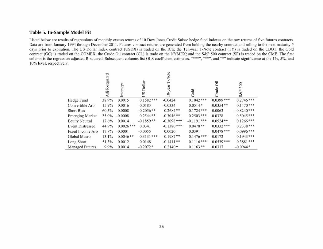
Before proceeding to the replication analysis, we examine the relation between hedge

fund index returns and those of the five futures contracts. For each index, we regress hedge fund

index returns in excess of the 1-month LIBOR rate on the raw returns of the five futures

contracts. The reason that we regress excess index returns on raw futures returns is that standard

cost-of-carry futures pricing models imply that futures returns do not reflect compensation for

the time value of money, whereas hedge fund index returns do. For this analysis we include an

12  

intercept, as is standard, so that regression coefficients and adjusted R-squared can be interpreted

in the usual way as we are interested here in assessing the in-sample fit of the factors.

Table 5 shows results using the full sample of 1994 through 2011. In-sample fit, as

measured by the adjusted R-squared of each regression, ranges from 9.9% for the Managed

Futures Index to 60.3% for the Short Bias Index, and averages 30.5% across the styles. These

low levels of fit are consistent with prior studies. One might be troubled by the low level of in-

sample fit for our indexes, since our ultimate goal is to generate a reasonable match out-of-

sample. Note, however, that in almost all cases the indexes feature a statistically significant

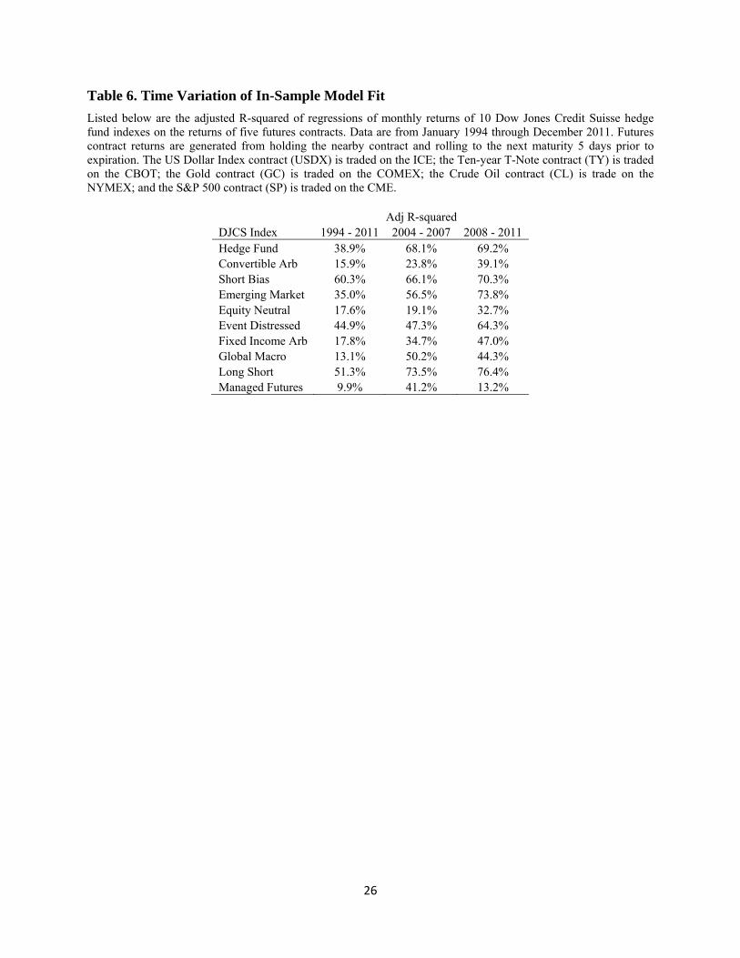
relation to four or five of the factors. More importantly, in-sample fit can be improved by

allowing for time varying exposures of the indexes to underlying factors, reflecting the trading

strategies of constituent fund managers. To illustrate, we report in Table 6 the adjusted R-

squared from regressions using two subsets of the data: 2004 – 2007 and 2008 – 2011. In many

cases the increase in adjusted R-squared as compared to the full sample is substantial. The Hedge

Fund Index, for example, features a 38.9% adjusted R-squared over the full sample as compared

to 68.1% and 69.2%, respectively, for the two latter periods. This result motivates our use of

rolling window estimation periods in the out-of-sample analysis.

4.2. Clone details

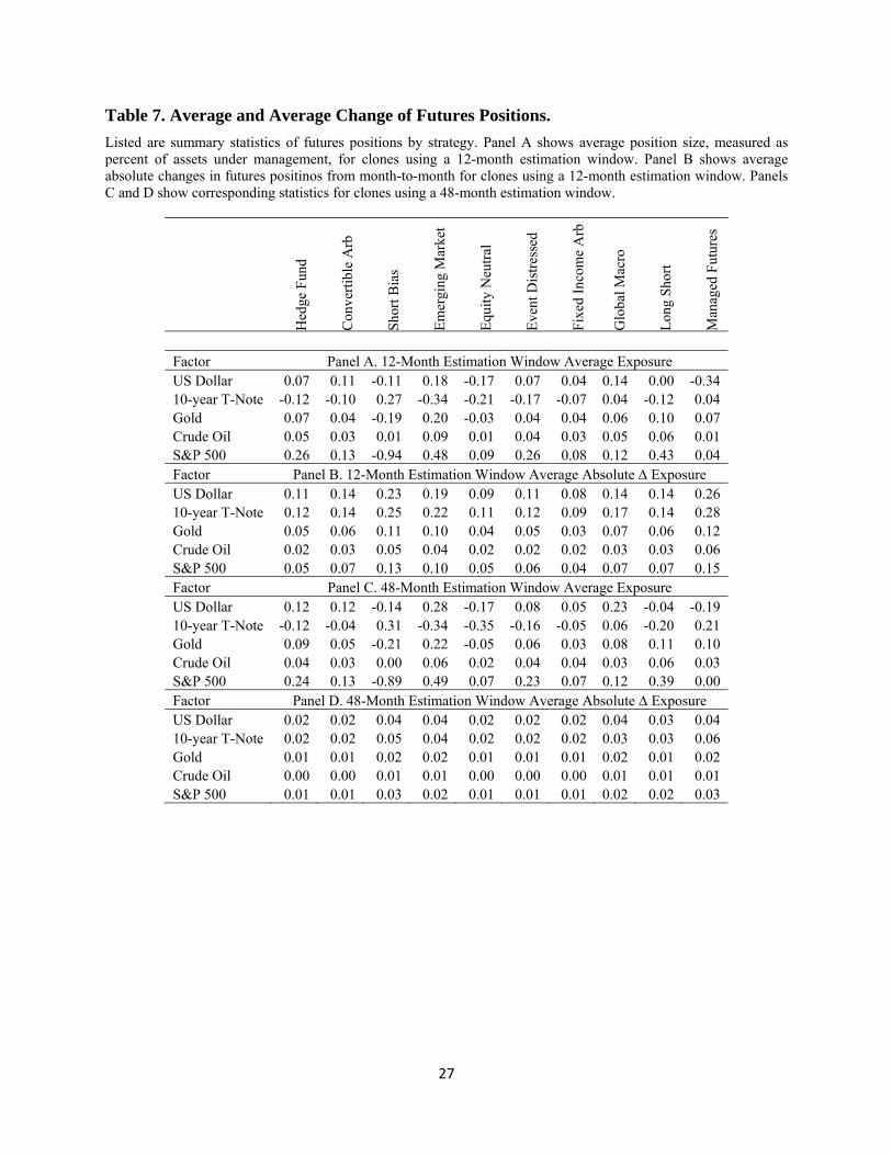
We present summary statistics of the exposures generated by the cloning algorithm

described in Section 3. The average position sizes and typical monthly changes are listed in

Table 7. Panels A and B show the average coefficient and the average absolute change in each

coefficient from month to month for the 12-month clone. The average positions in Panel A are

quite small, typically below 0.25 in absolute value, save for the ‒0.94 recorded on the S&P 500

factor for the Short Bias Index. The average absolute changes in Panel B, however, are

significant, often above 0.10. This means a typical month would involve a trade equal to 10% of

assets under management for each factor. Panels C and D show the corresponding statistics for

the 48-month estimation window. The average positions are comparable to the results in Panel A,

but the changes are much smaller, consistent with the idea that the estimated factor loading each

month is actually an average of a dynamic factor loading, hence the average will be more stable

the longer is the estimation window.

13  

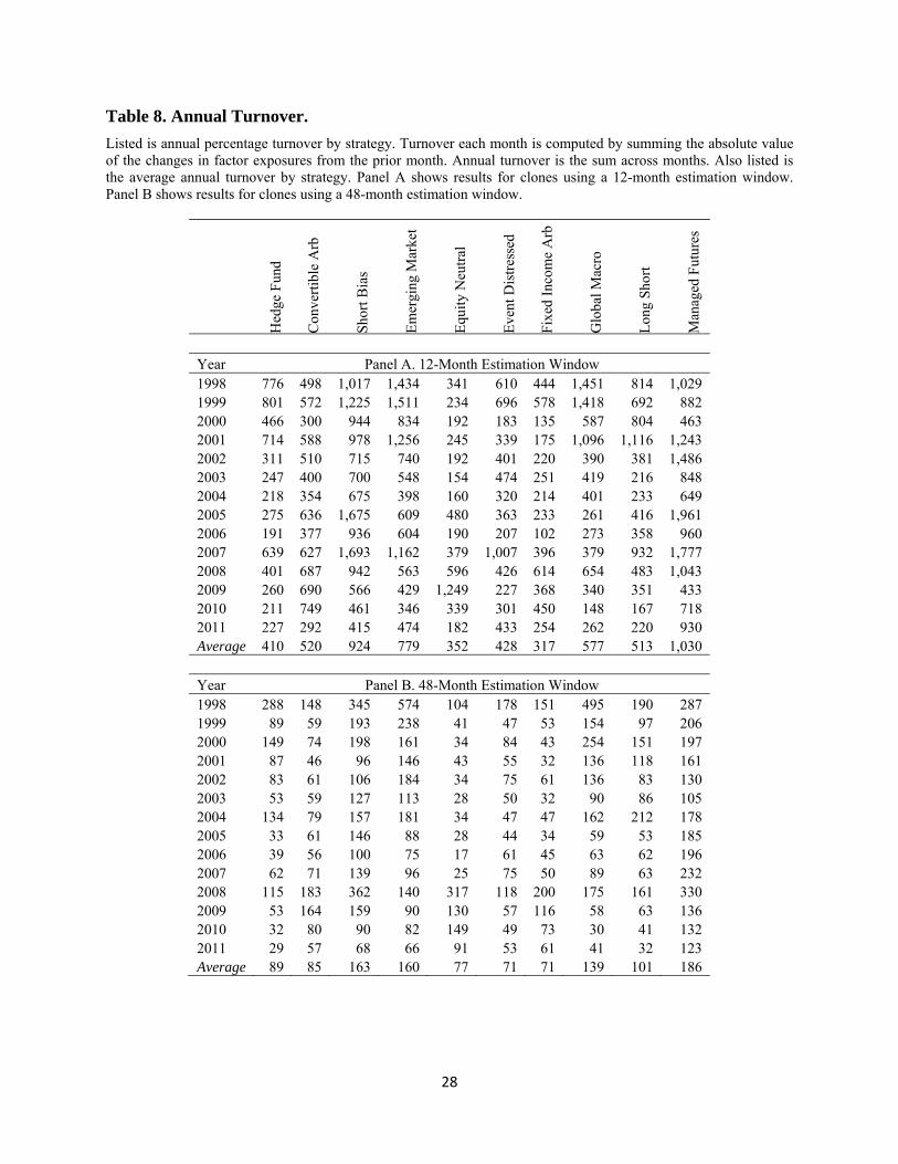
Table 8 shows the annual percentage turnover each year for each index. The annual

turnover equals the sum of the absolute value of the change in exposures each month. Panel A

shows the results for the 12-month estimation window. Several features stand out. First, there is

substantial variation across time and across indexes. High levels of turnover are observed around

the sharp climb and collapse of the dot-com era in 1998 and 2001, respectively. Turnover is also

high during the financial crisis years of 2007 – 2009. Turnover is highest for the Managed

Futures Index, averaging 1030% per year, and lowest for Fixed Income Arbitrage, at 317% per

year. Panel B shows results for the 48-month window. The time series patterns in turnover are

similar, but the magnitudes are much smaller. The Managed Futures Index is again the highest,

but with an average annual turnover of 186%. The Hedge Fund Index has an average turnover of

410% in Panel A but only 89% in Panel B, which is quite modest, similar to many mutual funds.

These results indicate that the length of the estimation window has a dramatic impact on

the size of positions as well as turnover, and is likely the most important variable for

implementing a cloning procedure.

4.3. Out-of-sample performance of clones

We measure the ability of clones to fit index returns out of sample by comparing the

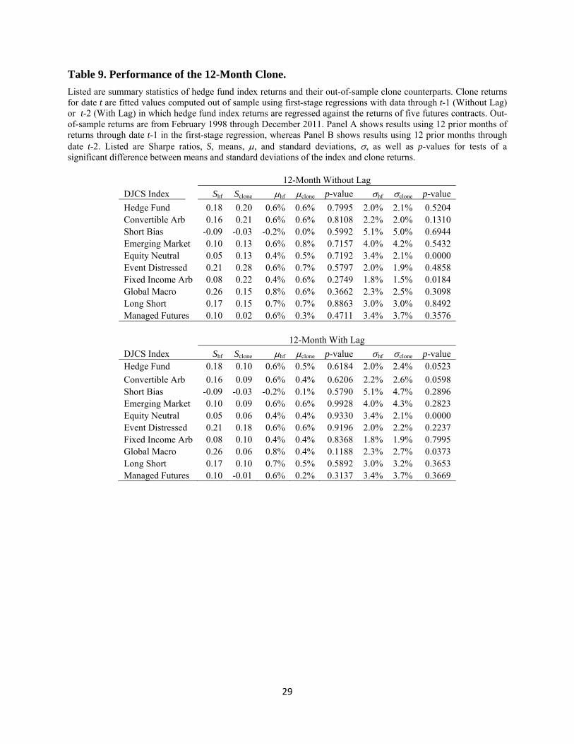
index returns to the clone returns from February 1998 through December 2011.5 Table 9 shows

results using 12-month estimation windows. Listed are monthly Sharpe ratios, average returns,

and standard deviations, as well as p-values of tests for a significant difference between the

averages and standard deviations of clones and indexes. Panel A lists statistics assuming no lag

between the end of the estimation period and the opening of futures positions necessary to

replicate the index. As described in Section 3, this is infeasible given that index returns are

typically not available until the 15th of a month, but the results show the hypothetical

performance in absence of this market friction. For the first seven indexes listed, the clones

deliver a higher Sharpe ratio than the index. The Hedge Fund Index delivers a Sharpe ratio of

0.18 compared to 0.20 for the clone, for example. In almost all cases there is no significant

difference between the average returns and standard deviations of the clones and the indexes. In

                                                            5 Since we use estimation windows up to 48 months long, data from 1994 through 1997 are used exclusively for measuring exposures. With a one-month lag, the first out-of-sample observation is February 1998.

14  

Panel B, however the clone performance weakens considerably with a one-month lag in portfolio

construction. For the Hedge Fund Index, for example, the Sharpe ratio drops to 0.10. This result

shows how implementation details are extremely important in determining the actual

performance of the replicating positions.

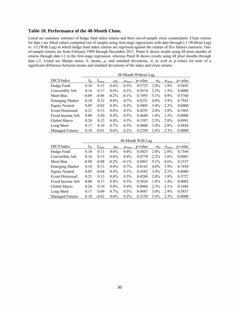
Table 10 shows results using a 48-month estimation period. Without a lag, four of the

clones deliver Sharpe ratios above their indexes, whereas three do with a one-month lag. In most

cases, however, average returns are not statistically significantly different across the clones and

indexes. In four of the clones, there is a significant difference in standard deviations, but in all

cases the clones have lower volatility. These results indicate that the clone performance may be

considered a reasonable alternative to the indexes.

Interestingly, a naïve strategy of maintaining equal weights on each of the five factors

generally outperforms the clones, and even the hedge fund indexes themselves. Over the same

time period as the results listed in Tables 9 and 10, a strategy of maintaining futures positions

each with notional value equal to 20% of assets under management, fully collateralized with

funds earning LIBOR, would have generated a monthly Sharpe ratio of over 0.22. This exceeds

all of the clones formed using the one-month lag. Naturally past performance is no guarantee of

future success, and events during the sample period were extreme by historical standards. That

said, the fact that an equally-weighted portfolio tends to outperform both the clones and the

targets suggests that simple alternatives may have merit.

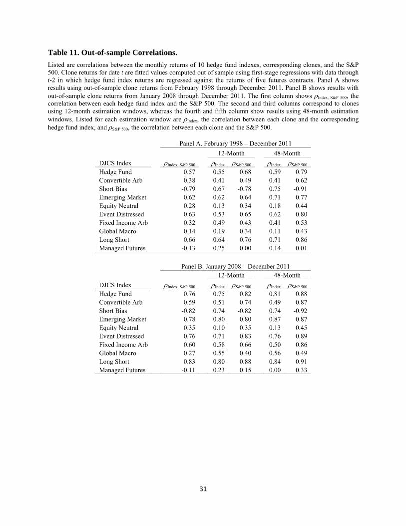
Table 11 provides some more insight regarding the match between the hedge fund

indexes and the corresponding clones. Listed are three types of correlations: the correlation

between each index and the S&P 500 total return, Index, S&P 500, the correlation between each

clone and the corresponding index, Index, and the correlation between each clone and the S&P

500, S&P 500. Panel A shows results using the full out-of-sample period February 1998 through

December 2011. The first column indicates the correlation between each index and the S&P 500.

The Long Short Index has the highest correlation of 0.66. The next two columns involve clones

that use a 12-month estimation window. Here the correlations between the clones and the

indexes are comparable to correlations between the indexes and the S&P 500. The Hedge Fund

Index, for example, features a correlation with the S&P 500 of 0.57, whereas its correlation with

the clone is 0.55. Note, however, that the correlation between the clone and the S&P 500 is

15  

higher, at 0.68. In most cases, this pattern is repeated. For the 48-month clone in the last two

columns, the correlation between the clones and the S&P 500 is generally higher still. This result

is unsettling because one of the primary reasons for seeking an alternative investment, or its

clone, is to achieve diversification from standard asset classes such as large cap U.S. equities.

Panel B of Table 11 shows correlations computed over the more recent period of 2008 –

2011. Here the correlations between clones and their indexes are higher than before, but the

correlation between clones and the S&P 500 often exceeds 0.80. In some respects this may not

be a big surprise. Risky assets in general became more highly correlated in the wake of the

financial crisis.

4.4. Market timing ability and dynamic factor loadings

The prior subsection shows that we do have some ability to match time series properties

of hedge fund indexes by using backward-looking rolling window regressions to estimate factor

loadings, and using these to establish portfolio weights going forward. However, the

performance of the clones is inferior to a simple strategy of equally weighting the five futures-

based factors. A remaining question is whether the poor performance of the clones is due to the

construction methodology, perhaps because the backward-looking estimates always provide stale

information, or is due to tracking a target which itself does not contain useful information

regarding future returns. As mentioned previously, the performance of the clones is completely

attributable to the dynamic nature of factor exposures inferred from the hedge fund indexes,

since the clones are constructed directly from the index factor loadings. Thus, to measure the

performance of the clones, and the indexes themselves, we assess their market timing

performance.

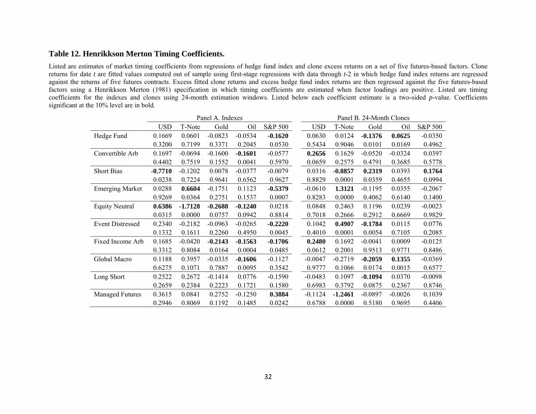
In Table 12, we list Henrikkson Merton timing coefficients for the indexes and the clone

with a 24-month estimation window.6 Listed below each coefficient is a two-sided p-value;

coefficients significant at the 10% level are in bold. As described in Section 3, positive

coefficients indicate that exposures are higher when factor returns are above zero, consistent with

timing ability, whereas negative coefficients indicate that exposures are lower when factor

                                                            6 Results for other estimation windows are qualitatively similar and omitted for the sake of brevity.

16  

returns are above zero. Panel A shows the results for the indexes. The vast majority of timing

coefficients are statistically insignificant. In 11 cases out of 50, the coefficients are significant

but negative, and in only three cases are they positive and significant. These results indicate the

indexes themselves do not feature successful time variation in factor loadings. Naturally, since

the indexes do not feature timing ability then it hardly seems likely that the clones would either.

Panel B confirms this: in six cases the coefficients are positive and significant and in six cases

the coefficients are negative and significant.

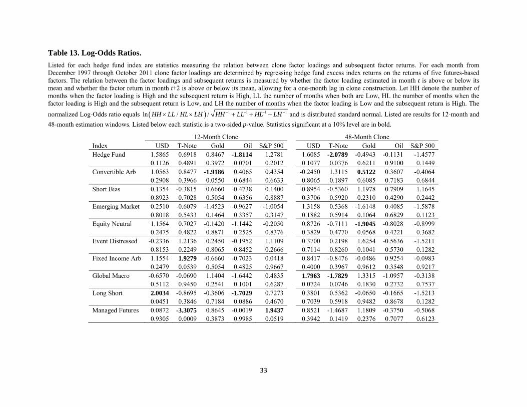
As discussed in Bollen and Busse (2001), regressions of market timing models tend to

lack power when using monthly data and results can be sensitive to the assumed functional form.

For this reason we also use a log-odds ratio for robustness. Here we count the number of months

in which factor loadings and subsequent returns are simultaneously above or below their mean,

and compare it to the number of months when factor loadings are high and returns are low or

vice versa. Table 13 shows the resulting log-odds ratios for each index and factor, for both the

12-month clone and the 48-month clone. A positive ratio indicates effective timing. Consistent

with the results of our Henrikkson Merton analysis, there is no evidence of market timing. The

number of positive and significant coefficients is equal to the number expected under the null

hypothesis of no ability, three for the case of the 12-month clone and two for the case of the 48-

month clone.

5. Conclusion

Hedge fund replication products constitute a relatively new choice for investors in their

pursuit of alternative investments. We analyze the performance of hedge fund clones constructed

by taking time varying positions in five liquid futures contracts. The targets we attempt to

replicate are the Credit Suisse hedge fund indexes.

Our results are mixed. On the one hand, we are able to construct clones with out-of-

sample correlations with their respective targets that exceed 0.50 for seven or eight of the

indexes, depending on the estimation window length chosen. The clone of the broad Hedge Fund

Index, for example, features a correlation with the index of 0.75 using a 12-month window and

0.81 with a 48-month window. On the other hand, the Sharpe ratios of clones are generally

inferior to those of the hedge fund indexes, and annual returns of clones are often below those of

17  

the indexes. Our ability to match the time-series properties of hedge fund indexes appears to be

largely the result of matching the exposure of the indexes to the equity market, which calls into

question the benefit of a supposedly alternative investment. In addition, standard market timing

regressions and log-odds ratio tests indicate that neither the clones nor the target indexes feature

market timing ability.

Despite the poor performance of the clones relative to the targets, there is still utility in

our replication procedure. For example, a portable alpha strategy, in which individual funds are

selected based on their potential for alpha generation, requires an algorithm for eliminating

systematic risk, as described in Kung and Pohlman (2004). Even market neutral funds can have

residual exposure, as shown in Patton (2009), hence the need for this type of hedging to make a

pure play on alpha generation. In the context of our study, the rolling window factor model

regressions indicate the size of the futures positions one should take to remove systematic risk

exposure. Such a strategy can aid risk budgeting for large institutional portfolios such as

university endowments and pension plans.

18  

References

Amenc, Noel, Walter Gehin, Lioinel Martellini, and Jean-Christophe Meyfredi. (2008) “Passive Hedge Fund Replication: A Critical Assessment of Existing Techniques” Journal of Alternative Investments, 69-83.

Amenc, Noel, Lioinel Martellini, and Jean-Christophe Meyfredi. (2010) “Passive Hedge Fund Replication – Beyond the Linear Case” European Financial Management 16, 191-210.

Amin, Gaurav, and Harry Kat. (2003) “Hedge Fund Performance 1990-2000: Do the ‘Money Machines’ Really Add Value?” Journal of Financial and Quantitative Analysis 38, 251-274.

Andrews, Donald W.K., Inpyo Lee, and Werner Ploberger. (1996) “Optimal Changepoint Tests for Normal Linear Regression” Journal of Econometrics 70, 9-38.

Bollen, Nicolas. (2012) “Zero-R2 Hedge Funds and Market Neutrality” Journal of Financial and Quantitative Analysis, forthcoming.

Bollen, Nicolas, and Jeffrey Busse. (2001) “On the Timing Ability of Mutual Fund Managers” Journal of Finance 56, 1075-1094.

Bollen, Nicolas, and Robert Whaley. (2009) “Hedge Fund Risk Dynamics: Implications for Performance Appraisal” Journal of Finance 59, 711-753.

Chen, Yong. (2007) “Timing Ability in the Focus Market of Hedge Funds” Journal of Investment Management 5, 66-98.

Chen, Yong, and Bing Liang. (2007) “Do Market Timing Hedge Funds Time the Market?” Journal of Financial and Quantitative Analysis 42, 827-856.

Dybvig, Peter (1988). “Distributional Analysis of Portfolio Choice” Journal of Business 61, 369-393.

Fung, William, and David Hsieh. (2001) “The Risk in Hedge Fund Strategies: Theory and Evidence from Trend Followers” Review of Financial Studies 14, 313-341.

Fung, William, and David Hsieh. (2004) “Hedge Fund Benchmarks: A Risk Based Approach” Financial Analysts Journal 60, 65-80.

Griffin, John, and Jin Xu. (2009) “How Smart are the Smart Guys? A Unique View from Hedge Fund Stock Holdings” Review of Financial Studies 22, 2531-2570.

Hasanhodzic, Jasmina, and Andrew Lo. (2007) “Can Hedge-Fund Returns be Replicated? The Linear Case” Journal of Investment Management 5, 5-45.

Henrikkson, Roy, and Robert Merton. (1981) “On Market Timing and Investment Performance of Managed Portfolios. II. Statistical Procedures for Evaluating Forecasting Skills” Journal of Business 54, 513-533.

Kat, Harry, and Helder Palaro. (2005) “Who Needs Hedge Funds? A Copula-Based Approach to Hedge Fund Return Replication” City University Working Paper.

Kung, Edward, and Larry Pohlman. (2004) “Portable Alpha” Journal of Portfolio Management 30, 78-87.

19  

Patton, Andrew. (2009) “Are Market Neutral Hedge Funds Really Market Neutral?” Review of Financial Studies 22, 2495-2530.

Patton, Andrew and Tarun Ramadorai. (2012) “On the High-Frequency Dynamics of Hedge Fund Risk Exposures” Journal of Finance, forthcoming.

Sharpe, William. (1992) “Asset allocation: Management style and performance measurement” Journal of Portfolio Management, 7-19.

Treynor, Jack, and Kay Mazuy. (1966) “Can Mutual Funds Outguess the Market?” Harvard Business Review 44, 131-136.

20  

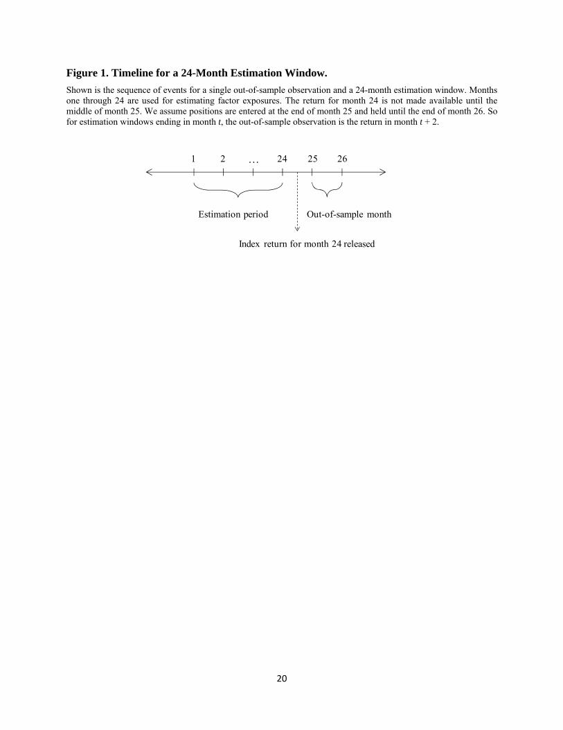
Figure 1. Timeline for a 24-Month Estimation Window.

Shown is the sequence of events for a single out-of-sample observation and a 24-month estimation window. Months one through 24 are used for estimating factor exposures. The return for month 24 is not made available until the middle of month 25. We assume positions are entered at the end of month 25 and held until the end of month 26. So for estimation windows ending in month t, the out-of-sample observation is the return in month t + 2.

1 2 … 24 25 26

Estimation period Out-of-sample month

Index return for month 24 released

21  

Table 1. Summary Statistics of Hedge Fund Indexes.

Listed below are summary statistics of monthly returns of 10 Dow Jones Credit Suisse hedge fund indexes and the total return of the S&P 500 index. Data are from January 1994 through December 2011. The first three statistics are annualized. “Sharpe” is the Sharpe ratio, defined as the average return in excess of the 30-day T-Bill rate divided by standard deviation; “Skew” is skewness; “Kurt” is excess kurtosis; “% Neg” is the percentage of months with a negative return; and “S&P 500” is the correlation coefficient between an index and the S&P 500.

DJCS Index Average Std Dev Sharpe Skew Kurt % Neg S&P 500 Hedge Fund 8.6% 7.6% 0.73 -0.19 2.42 29.6% 0.57 Convertible Arb 7.4% 7.0% 0.62 -2.68 15.96 25.5% 0.37 Short Bias -2.0% 17.0% -0.30 0.65 1.44 55.1% -0.76 Emerging Market 8.3% 15.0% 0.34 -0.76 5.03 38.0% 0.54 Equity Neutral 5.6% 10.4% 0.24 -11.85 161.12 20.4% 0.29 Event Distressed 9.0% 6.4% 0.93 -2.24 10.64 23.2% 0.63 Fixed Income Arb 5.3% 5.8% 0.37 -4.39 30.39 21.8% 0.33 Global Macro 12.0% 9.8% 0.90 0.00 3.78 26.9% 0.24 Long Short 9.4% 10.0% 0.62 0.00 3.25 35.2% 0.66 Managed Futures 6.5% 11.8% 0.29 0.02 -0.03 44.9% -0.10 S&P 500 8.9% 15.7% 0.37 -0.63 0.90 37.5%

22  

Table 2. Summary Statistics of Hedge Fund Indexes.

Listed below are summary statistics of monthly returns of 10 Dow Jones Credit Suisse hedge fund indexes and the total return of the S&P 500 index. Statistics are computed over three periods: January 1994 through December 2003 (Panel A), January 2004 through December 2007 (Panel B), and January 2008 through December 2011 (Panel C). The first three statistics are annualized. “Sharpe” is the Sharpe ratio, defined as the average return in excess of the 30-day T-Bill rate divided by standard deviation; “Skew” is skewness; “Kurt” is excess kurtosis; “% Neg” is the percentage of months with a negative return; and “S&P 500” is the correlation coefficient between an index and the S&P 500.

Panel A. 1994 - 2003

DJCS Index Average Std Dev Sharpe Skew Kurt % Neg S&P 500 Hedge Fund 10.9% 8.5% 0.81 0.08 1.73 29.2% 0.48 Convertible Arb 10.1% 4.8% 1.26 -1.57 4.06 18.3% 0.12 Short Bias -1.7% 18.0% -0.32 0.92 2.15 55.0% -0.76 Emerging Market 8.5% 17.8% 0.25 -0.58 3.71 40.8% 0.48 Equity Neutral 10.2% 3.1% 1.99 0.21 0.24 15.8% 0.39 Event Distressed 11.0% 6.0% 1.15 -3.46 22.95 20.0% 0.55 Fixed Income Arb 6.7% 3.9% 0.65 -3.25 16.61 18.3% 0.03 Global Macro 14.3% 12.1% 0.84 -0.04 1.98 29.2% 0.23 Long Short 12.1% 11.0% 0.73 0.22 3.35 33.3% 0.59 Managed Futures 7.6% 12.1% 0.29 0.03 0.58 44.2% -0.23 S&P 500 12.0% 15.8% 0.50 -0.59 0.26 36.7%

Panel B. 2004 - 2007

DJCS Index Average Std Dev Sharpe Skew Kurt % Neg S&P 500 Hedge Fund 10.4% 4.2% 1.71 -0.17 -0.55 22.9% 0.68 Convertible Arb 4.6% 3.9% 0.30 -0.73 0.92 33.3% 0.41 Short Bias 2.5% 13.4% -0.06 0.49 0.08 52.1% -0.81 Emerging Market 16.6% 7.6% 1.76 -0.76 1.05 20.8% 0.48 Equity Neutral 7.9% 2.0% 2.28 0.47 0.12 10.4% 0.15 Event Distressed 12.4% 4.0% 2.28 -0.49 0.85 10.4% 0.62 Fixed Income Arb 4.9% 2.7% 0.55 -0.59 0.73 25.0% 0.27 Global Macro 11.5% 3.7% 2.22 0.57 0.81 16.7% 0.40 Long Short 11.9% 6.0% 1.43 -0.35 -0.78 27.1% 0.75 Managed Futures 5.5% 11.5% 0.18 -0.08 -0.89 43.8% 0.62 S&P 500 9.2% 7.6% 0.78 -0.37 -0.70 31.3%

Panel C. 2008 - 2011

DJCS Index Average Std Dev Sharpe Skew Kurt % Neg S&P 500 Hedge Fund 1.2% 7.8% 0.10 -1.05 1.49 37.5% 0.76 Convertible Arb 3.8% 12.1% 0.28 -1.94 6.15 35.4% 0.59 Short Bias -7.6% 17.7% -0.45 0.08 -0.63 58.3% -0.82 Emerging Market -0.7% 12.7% -0.09 -1.28 3.40 47.9% 0.78 Equity Neutral -8.0% 21.2% -0.40 -6.11 40.35 41.7% 0.36 Event Distressed 0.7% 8.4% 0.03 -0.71 0.11 43.8% 0.76 Fixed Income Arb 2.2% 10.2% 0.17 -3.02 11.69 27.1% 0.60 Global Macro 6.5% 7.1% 0.85 -1.12 2.87 31.3% 0.27 Long Short -0.2% 10.1% -0.07 -0.59 0.28 47.9% 0.83 Managed Futures 4.9% 11.3% 0.39 0.07 -1.11 47.9% -0.11 S&P 500 0.6% 20.5% 0.01 -0.44 0.06 45.8%

23  

Table 3. Summary Statistics of Futures Contracts.

Listed below are summary statistics of monthly returns of five futures contracts used to build clones for hedge fund indexes. Data are from January 1994 through December 2011. Futures contract returns are generated from holding the nearby contract and rolling to the next maturity 5 days prior to expiration. The US Dollar Index contract (USDX) is traded on the ICE; the Ten-year T-Note contract (TY) is traded on the CBOT; the Gold contract (GC) is traded on the COMEX; the Crude Oil contract (CL) is trade on the NYMEX; and the S&P 500 contract (SP) is traded on the CME. The first three statistics are annualized. “Sharpe” is the Sharpe ratio, defined for futures returns as the average return divided by standard deviation; “Skew” is skewness; “Kurt” is excess kurtosis; “% Neg” is the percentage of months with a negative return; and “S&P 500” is the correlation coefficient between an index and the S&P 500.

Panel A. 1994 - 2011

Futures Contract Average Std Dev Sharpe Skew Kurt % Neg S&P 500 US Dollar -0.7% 8.3% -0.09 0.34 0.74 52.3% -0.25 10-year T-Note 1.1% 7.0% 0.16 -0.92 6.99 45.8% -0.15 Gold 9.0% 16.1% 0.56 0.14 1.43 46.3% 0.02 Crude Oil 16.1% 32.3% 0.50 -0.05 1.12 41.7% 0.19 S&P 500 6.7% 15.8% 0.43 -0.64 0.99 38.9%

Panel B. 1994 - 2003

Futures Contract Average Std Dev Sharpe Skew Kurt % Neg S&P 500 US Dollar -0.8% 7.7% -0.11 0.11 -0.08 53.3% 0.03 10-year T-Note 0.2% 7.4% 0.03 -1.73 8.29 46.7% -0.09 Gold 1.3% 12.3% 0.11 1.00 2.66 50.8% -0.06 Crude Oil 13.3% 32.0% 0.42 0.26 1.21 43.3% 0.01 S&P 500 10.0% 16.0% 0.62 -0.58 0.36 37.5%

Panel C. 2004 - 2007

Futures Contract Average Std Dev Sharpe Skew Kurt % Neg S&P 500 US Dollar -3.0% 6.1% -0.50 0.04 0.08 50.0% -0.23 10-year T-Note 0.4% 5.0% 0.07 -0.28 0.71 47.9% -0.26 Gold 18.7% 15.4% 1.21 0.24 -0.04 43.8% 0.17 Crude Oil 31.1% 27.7% 1.12 -0.04 -0.97 41.7% -0.17 S&P 500 7.4% 7.7% 0.97 -0.50 -0.50 31.3%

Panel D. 2008 - 2011

Futures Contract Average Std Dev Sharpe Skew Kurt % Neg S&P 500 US Dollar 1.8% 11.3% 0.16 0.42 0.23 52.1% -0.63 10-year T-Note 4.0% 7.7% 0.51 0.74 3.11 41.7% -0.21 Gold 18.4% 23.0% 0.80 -0.57 0.47 37.5% 0.09 Crude Oil 7.8% 37.2% 0.21 -0.45 1.48 37.5% 0.61 S&P 500 -1.9% 20.7% -0.10 -0.47 0.12 50.0%

24  

Table 4. Correlations of Futures Contracts.

Listed below are correlations of monthly returns of five futures contracts used to build clones for hedge fund indexes. Data are from January 1994 through December 2011. Futures contract returns are generated from holding the nearby contract and rolling to the next maturity 5 days prior to expiration. The US Dollar Index contract (USDX) is traded on the ICE; the Ten-year T-Note contract (TY) is traded on the CBOT; the Gold contract (GC) is traded on the COMEX; the Crude Oil contract (CL) is trade on the NYMEX; and the S&P 500 contract (SP) is traded on the CME.

1994 - 2011

US

Dol

lar

10-y

ear

T-N

ote

Gol

d

Cru

de O

il

S&

P 5

00

US Dollar 1.00 10-year T-Note -0.11 1.00 Gold -0.44 0.19 1.00 Crude Oil -0.29 -0.11 0.20 1.00 S&P 500 -0.25 -0.15 0.02 0.19 1.00

2004 - 2007

US

Dol

lar

10-y

ear

T-N

ote

Gol

d

Cru

de O

il

S&

P 5

00

US Dollar 1.00 10-year T-Note -0.13 1.00 Gold -0.55 0.06 1.00 Crude Oil -0.20 -0.03 0.22 1.00 S&P 500 -0.23 -0.26 0.17 -0.17 1.00

2008 - 2011

US

Dol

lar

10-y

ear

T-N

ote

Gol

d

Cru

de O

il

S&

P 5

00

US Dollar 1.00 10-year T-Note -0.11 1.00 Gold -0.49 0.41 1.00 Crude Oil -0.54 -0.38 0.22 1.00 S&P 500 -0.63 -0.21 0.09 0.61 1.00

25  

Table 5. In-Sample Model Fit

Listed below are results of regressions of monthly excess returns of 10 Dow Jones Credit Suisse hedge fund indexes on the raw returns of five futures contracts. Data are from January 1994 through December 2011. Futures contract returns are generated from holding the nearby contract and rolling to the next maturity 5 days prior to expiration. The US Dollar Index contract (USDX) is traded on the ICE; the Ten-year T-Note contract (TY) is traded on the CBOT; the Gold contract (GC) is traded on the COMEX; the Crude Oil contract (CL) is trade on the NYMEX; and the S&P 500 contract (SP) is traded on the CME. The first column is the regression adjusted R-squared. Subsequent columns list OLS coefficient estimates. “***”, “**”, and “*” indicate significance at the 1%, 5%, and 10% level, respectively.

Adj

R-s

quar

ed

Inte

rcep

t

US

Dol

lar

10-y

ear

T-N

ote

Gol

d

Cru

de O

il

S&

P 5

00

Hedge Fund 38.9% 0.0015 0.1582 *** -0.0424 0.1042 *** 0.0399 *** 0.2746 *** Convertible Arb 15.9% 0.0016 0.0183 -0.0334 0.0514 * 0.0354 ** 0.1470 *** Short Bias 60.3% 0.0008 -0.2056 ** 0.2684 ** -0.1724 *** 0.0063 -0.8240 *** Emerging Market 35.0% -0.0008 0.2544 ** -0.3046 ** 0.2503 *** 0.0328 0.5045 *** Equity Neutral 17.6% 0.0014 -0.1859 ** -0.3098 *** -0.1191 *** 0.0524 ** 0.1266 *** Event Distressed 44.9% 0.0026 *** 0.0341 -0.1380 *** 0.0478 ** 0.0332 *** 0.2338 *** Fixed Income Arb 17.8% -0.0001 -0.0055 0.0020 0.0391 0.0478 *** 0.0996 *** Global Macro 13.1% 0.0046 ** 0.3131 *** 0.1987 ** 0.1476 *** 0.0172 0.1943 *** Long Short 51.3% 0.0012 0.0148 -0.1411 ** 0.1116 *** 0.0539 *** 0.3881 *** Managed Futures 9.9% 0.0014 -0.2072 * 0.2140 * 0.1163 ** 0.0317 -0.0944 *

 

26  

Table 6. Time Variation of In-Sample Model Fit

Listed below are the adjusted R-squared of regressions of monthly returns of 10 Dow Jones Credit Suisse hedge fund indexes on the returns of five futures contracts. Data are from January 1994 through December 2011. Futures contract returns are generated from holding the nearby contract and rolling to the next maturity 5 days prior to expiration. The US Dollar Index contract (USDX) is traded on the ICE; the Ten-year T-Note contract (TY) is traded on the CBOT; the Gold contract (GC) is traded on the COMEX; the Crude Oil contract (CL) is trade on the NYMEX; and the S&P 500 contract (SP) is traded on the CME.

Adj R-squared DJCS Index 1994 - 2011 2004 - 2007 2008 - 2011 Hedge Fund 38.9% 68.1% 69.2% Convertible Arb 15.9% 23.8% 39.1% Short Bias 60.3% 66.1% 70.3% Emerging Market 35.0% 56.5% 73.8% Equity Neutral 17.6% 19.1% 32.7% Event Distressed 44.9% 47.3% 64.3% Fixed Income Arb 17.8% 34.7% 47.0% Global Macro 13.1% 50.2% 44.3% Long Short 51.3% 73.5% 76.4% Managed Futures 9.9% 41.2% 13.2%

   

27  

Table 7. Average and Average Change of Futures Positions.

Listed are summary statistics of futures positions by strategy. Panel A shows average position size, measured as percent of assets under management, for clones using a 12-month estimation window. Panel B shows average absolute changes in futures positinos from month-to-month for clones using a 12-month estimation window. Panels C and D show corresponding statistics for clones using a 48-month estimation window.

Hed

ge F

und

Con

vert

ible

Arb

Sho

rt B

ias

Em

ergi

ng M

arke

t

Equ

ity N

eutr

al

Eve

nt D

istr

esse

d

Fixe

d In

com

e A

rb

Glo

bal M

acro

Lon

g Sh

ort

Man

aged

Fut

ures

Factor Panel A. 12-Month Estimation Window Average Exposure US Dollar 0.07 0.11 -0.11 0.18 -0.17 0.07 0.04 0.14 0.00 -0.34 10-year T-Note -0.12 -0.10 0.27 -0.34 -0.21 -0.17 -0.07 0.04 -0.12 0.04 Gold 0.07 0.04 -0.19 0.20 -0.03 0.04 0.04 0.06 0.10 0.07 Crude Oil 0.05 0.03 0.01 0.09 0.01 0.04 0.03 0.05 0.06 0.01 S&P 500 0.26 0.13 -0.94 0.48 0.09 0.26 0.08 0.12 0.43 0.04 Factor Panel B. 12-Month Estimation Window Average Absolute Exposure US Dollar 0.11 0.14 0.23 0.19 0.09 0.11 0.08 0.14 0.14 0.26 10-year T-Note 0.12 0.14 0.25 0.22 0.11 0.12 0.09 0.17 0.14 0.28 Gold 0.05 0.06 0.11 0.10 0.04 0.05 0.03 0.07 0.06 0.12 Crude Oil 0.02 0.03 0.05 0.04 0.02 0.02 0.02 0.03 0.03 0.06 S&P 500 0.05 0.07 0.13 0.10 0.05 0.06 0.04 0.07 0.07 0.15 Factor Panel C. 48-Month Estimation Window Average Exposure US Dollar 0.12 0.12 -0.14 0.28 -0.17 0.08 0.05 0.23 -0.04 -0.19 10-year T-Note -0.12 -0.04 0.31 -0.34 -0.35 -0.16 -0.05 0.06 -0.20 0.21 Gold 0.09 0.05 -0.21 0.22 -0.05 0.06 0.03 0.08 0.11 0.10 Crude Oil 0.04 0.03 0.00 0.06 0.02 0.04 0.04 0.03 0.06 0.03 S&P 500 0.24 0.13 -0.89 0.49 0.07 0.23 0.07 0.12 0.39 0.00 Factor Panel D. 48-Month Estimation Window Average Absolute Exposure US Dollar 0.02 0.02 0.04 0.04 0.02 0.02 0.02 0.04 0.03 0.04 10-year T-Note 0.02 0.02 0.05 0.04 0.02 0.02 0.02 0.03 0.03 0.06 Gold 0.01 0.01 0.02 0.02 0.01 0.01 0.01 0.02 0.01 0.02 Crude Oil 0.00 0.00 0.01 0.01 0.00 0.00 0.00 0.01 0.01 0.01 S&P 500 0.01 0.01 0.03 0.02 0.01 0.01 0.01 0.02 0.02 0.03

28  

Table 8. Annual Turnover.

Listed is annual percentage turnover by strategy. Turnover each month is computed by summing the absolute value of the changes in factor exposures from the prior month. Annual turnover is the sum across months. Also listed is the average annual turnover by strategy. Panel A shows results for clones using a 12-month estimation window. Panel B shows results for clones using a 48-month estimation window.

Hed

ge F

und

Con

vert

ible

Arb

Sho

rt B

ias

Em

ergi

ng M

arke

t

Equ

ity N

eutr

al

Eve

nt D

istr

esse

d

Fixe

d In

com

e A

rb

Glo

bal M

acro

Lon

g Sh

ort

Man

aged

Fut

ures

Year Panel A. 12-Month Estimation Window 1998 776 498 1,017 1,434 341 610 444 1,451 814 1,029 1999 801 572 1,225 1,511 234 696 578 1,418 692 882 2000 466 300 944 834 192 183 135 587 804 463 2001 714 588 978 1,256 245 339 175 1,096 1,116 1,243 2002 311 510 715 740 192 401 220 390 381 1,486 2003 247 400 700 548 154 474 251 419 216 848 2004 218 354 675 398 160 320 214 401 233 649 2005 275 636 1,675 609 480 363 233 261 416 1,961 2006 191 377 936 604 190 207 102 273 358 960 2007 639 627 1,693 1,162 379 1,007 396 379 932 1,777 2008 401 687 942 563 596 426 614 654 483 1,043 2009 260 690 566 429 1,249 227 368 340 351 433 2010 211 749 461 346 339 301 450 148 167 718 2011 227 292 415 474 182 433 254 262 220 930 Average 410 520 924 779 352 428 317 577 513 1,030

Year Panel B. 48-Month Estimation Window 1998 288 148 345 574 104 178 151 495 190 287 1999 89 59 193 238 41 47 53 154 97 206 2000 149 74 198 161 34 84 43 254 151 197 2001 87 46 96 146 43 55 32 136 118 161 2002 83 61 106 184 34 75 61 136 83 130 2003 53 59 127 113 28 50 32 90 86 105 2004 134 79 157 181 34 47 47 162 212 178 2005 33 61 146 88 28 44 34 59 53 185 2006 39 56 100 75 17 61 45 63 62 196 2007 62 71 139 96 25 75 50 89 63 232 2008 115 183 362 140 317 118 200 175 161 330 2009 53 164 159 90 130 57 116 58 63 136 2010 32 80 90 82 149 49 73 30 41 132 2011 29 57 68 66 91 53 61 41 32 123 Average 89 85 163 160 77 71 71 139 101 186

29  

Table 9. Performance of the 12-Month Clone.

Listed are summary statistics of hedge fund index returns and their out-of-sample clone counterparts. Clone returns for date t are fitted values computed out of sample using first-stage regressions with data through t-1 (Without Lag) or t-2 (With Lag) in which hedge fund index returns are regressed against the returns of five futures contracts. Out-of-sample returns are from February 1998 through December 2011. Panel A shows results using 12 prior months of returns through date t-1 in the first-stage regression, whereas Panel B shows results using 12 prior months through date t-2. Listed are Sharpe ratios, S, means, , and standard deviations, , as well as p-values for tests of a significant difference between means and standard deviations of the index and clone returns.

12-Month Without Lag

DJCS Index Shf Sclone hf clone p-value hf clone p-value

Hedge Fund 0.18 0.20 0.6% 0.6% 0.7995 2.0% 2.1% 0.5204 Convertible Arb 0.16 0.21 0.6% 0.6% 0.8108 2.2% 2.0% 0.1310 Short Bias -0.09 -0.03 -0.2% 0.0% 0.5992 5.1% 5.0% 0.6944 Emerging Market 0.10 0.13 0.6% 0.8% 0.7157 4.0% 4.2% 0.5432 Equity Neutral 0.05 0.13 0.4% 0.5% 0.7192 3.4% 2.1% 0.0000 Event Distressed 0.21 0.28 0.6% 0.7% 0.5797 2.0% 1.9% 0.4858 Fixed Income Arb 0.08 0.22 0.4% 0.6% 0.2749 1.8% 1.5% 0.0184 Global Macro 0.26 0.15 0.8% 0.6% 0.3662 2.3% 2.5% 0.3098 Long Short 0.17 0.15 0.7% 0.7% 0.8863 3.0% 3.0% 0.8492 Managed Futures 0.10 0.02 0.6% 0.3% 0.4711 3.4% 3.7% 0.3576

12-Month With Lag

DJCS Index Shf Sclone hf clone p-value hf clone p-value Hedge Fund 0.18 0.10 0.6% 0.5% 0.6184 2.0% 2.4% 0.0523

Convertible Arb 0.16 0.09 0.6% 0.4% 0.6206 2.2% 2.6% 0.0598 Short Bias -0.09 -0.03 -0.2% 0.1% 0.5790 5.1% 4.7% 0.2896 Emerging Market 0.10 0.09 0.6% 0.6% 0.9928 4.0% 4.3% 0.2823 Equity Neutral 0.05 0.06 0.4% 0.4% 0.9330 3.4% 2.1% 0.0000 Event Distressed 0.21 0.18 0.6% 0.6% 0.9196 2.0% 2.2% 0.2237 Fixed Income Arb 0.08 0.10 0.4% 0.4% 0.8368 1.8% 1.9% 0.7995 Global Macro 0.26 0.06 0.8% 0.4% 0.1188 2.3% 2.7% 0.0373 Long Short 0.17 0.10 0.7% 0.5% 0.5892 3.0% 3.2% 0.3653 Managed Futures 0.10 -0.01 0.6% 0.2% 0.3137 3.4% 3.7% 0.3669

30  

Table 10. Performance of the 48-Month Clone.

Listed are summary statistics of hedge fund index returns and their out-of-sample clone counterparts. Clone returns for date t are fitted values computed out of sample using first-stage regressions with data through t-1 (Without Lag) or t-2 (With Lag) in which hedge fund index returns are regressed against the returns of five futures contracts. Out-of-sample returns are from February 1998 through December 2011. Panel A shows results using 48 prior months of returns through date t-1 in the first-stage regression, whereas Panel B shows results using 48 prior months through date t-2. Listed are Sharpe ratios, S, means, , and standard deviations, , as well as p-values for tests of a significant difference between means and standard deviations of the index and clone returns.

48-Month Without Lag

DJCS Index Shf Sclone hf clone p-value hf clone p-value Hedge Fund 0.18 0.12 0.6% 0.5% 0.5725 2.0% 1.9% 0.5493 Convertible Arb 0.16 0.17 0.6% 0.5% 0.5674 2.2% 1.5% 0.0000 Short Bias -0.09 -0.06 -0.2% -0.1% 0.7493 5.1% 4.9% 0.5760 Emerging Market 0.10 0.12 0.6% 0.7% 0.8231 4.0% 3.9% 0.7543 Equity Neutral 0.05 -0.02 0.4% 0.2% 0.5005 3.4% 2.2% 0.0000 Event Distressed 0.21 0.13 0.6% 0.5% 0.4255 2.0% 1.8% 0.1965 Fixed Income Arb 0.08 0.20 0.4% 0.5% 0.4688 1.8% 1.3% 0.0000 Global Macro 0.26 0.12 0.8% 0.5% 0.1397 2.3% 2.0% 0.0991 Long Short 0.17 0.10 0.7% 0.5% 0.4800 3.0% 2.8% 0.4844 Managed Futures 0.10 -0.01 0.6% 0.2% 0.2258 3.4% 2.3% 0.0000

48-Month With Lag

DJCS Index Shf Sclone hf clone p-value hf clone p-value Hedge Fund 0.18 0.11 0.6% 0.4% 0.5025 2.0% 2.0% 0.7544 Convertible Arb 0.16 0.13 0.6% 0.4% 0.4770 2.2% 1.6% 0.0001 Short Bias -0.09 -0.08 -0.2% -0.1% 0.8467 5.1% 4.6% 0.2157 Emerging Market 0.10 0.13 0.6% 0.7% 0.8142 4.0% 3.9% 0.7450 Equity Neutral 0.05 -0.04 0.4% 0.1% 0.4382 3.4% 2.2% 0.0000 Event Distressed 0.21 0.13 0.6% 0.5% 0.4288 2.0% 1.8% 0.3727 Fixed Income Arb 0.08 0.17 0.4% 0.5% 0.5826 1.8% 1.4% 0.0002 Global Macro 0.26 0.10 0.8% 0.4% 0.0960 2.3% 2.1% 0.1488 Long Short 0.17 0.09 0.7% 0.5% 0.4687 3.0% 2.9% 0.5857 Managed Futures 0.10 -0.02 0.6% 0.2% 0.2150 3.4% 2.3% 0.0000

31  

Table 11. Out-of-sample Correlations.

Listed are correlations between the monthly returns of 10 hedge fund indexes, corresponding clones, and the S&P 500. Clone returns for date t are fitted values computed out of sample using first-stage regressions with data through t-2 in which hedge fund index returns are regressed against the returns of five futures contracts. Panel A shows results using out-of-sample clone returns from February 1998 through December 2011. Panel B shows results with out-of-sample clone returns from January 2008 through December 2011. The first column shows Index, S&P 500, the correlation between each hedge fund index and the S&P 500. The second and third columns correspond to clones using 12-month estimation windows, whereas the fourth and fifth column show results using 48-month estimation windows. Listed for each estimation window are Index, the correlation between each clone and the corresponding hedge fund index, and S&P 500, the correlation between each clone and the S&P 500.

Panel A. February 1998 – December 2011

12-Month 48-Month

DJCS Index Index, S&P 500 Index S&P 500 Index S&P 500Hedge Fund 0.57 0.55 0.68 0.59 0.79 Convertible Arb 0.38 0.41 0.49 0.41 0.62 Short Bias -0.79 0.67 -0.78 0.75 -0.91 Emerging Market 0.62 0.62 0.64 0.71 0.77 Equity Neutral 0.28 0.13 0.34 0.18 0.44 Event Distressed 0.63 0.53 0.65 0.62 0.80 Fixed Income Arb 0.32 0.49 0.43 0.41 0.53 Global Macro 0.14 0.19 0.34 0.11 0.43 Long Short 0.66 0.64 0.76 0.71 0.86 Managed Futures -0.13 0.25 0.00 0.14 0.01

Panel B. January 2008 – December 2011 12-Month 48-Month

DJCS Index Index, S&P 500 Index S&P 500 Index S&P 500Hedge Fund 0.76 0.75 0.82 0.81 0.88 Convertible Arb 0.59 0.51 0.74 0.49 0.87 Short Bias -0.82 0.74 -0.82 0.74 -0.92 Emerging Market 0.78 0.80 0.80 0.87 0.87 Equity Neutral 0.35 0.10 0.35 0.13 0.45 Event Distressed 0.76 0.71 0.83 0.76 0.89 Fixed Income Arb 0.60 0.58 0.66 0.50 0.86 Global Macro 0.27 0.55 0.40 0.56 0.49 Long Short 0.83 0.80 0.88 0.84 0.91 Managed Futures -0.11 0.23 0.15 0.00 0.33

32  

Table 12. Henrikkson Merton Timing Coefficients.

Listed are estimates of market timing coefficients from regressions of hedge fund index and clone excess returns on a set of five futures-based factors. Clone returns for date t are fitted values computed out of sample using first-stage regressions with data through t-2 in which hedge fund index returns are regressed against the returns of five futures contracts. Excess fitted clone returns and excess hedge fund index returns are then regressed against the five futures-based factors using a Henrikkson Merton (1981) specification in which timing coefficients are estimated when factor loadings are positive. Listed are timing coefficients for the indexes and clones using 24-month estimation windows. Listed below each coefficient estimate is a two-sided p-value. Coefficients significant at the 10% level are in bold.

Panel A. Indexes Panel B. 24-Month Clones USD T-Note Gold Oil S&P 500 USD T-Note Gold Oil S&P 500 Hedge Fund 0.1669 0.0601 -0.0823 -0.0534 -0.1620 0.0630 0.0124 -0.1376 0.0625 -0.0350 0.3200 0.7199 0.3371 0.2045 0.0530 0.5434 0.9046 0.0101 0.0169 0.4962 Convertible Arb 0.1697 -0.0694 -0.1600 -0.1601 -0.0577 0.2656 0.1629 -0.0520 -0.0324 0.0397 0.4402 0.7519 0.1552 0.0041 0.5970 0.0659 0.2575 0.4791 0.3685 0.5778 Short Bias -0.7710 -0.1202 0.0078 -0.0377 -0.0079 0.0316 -0.8857 0.2319 0.0393 0.1764 0.0238 0.7224 0.9641 0.6562 0.9627 0.8829 0.0001 0.0359 0.4655 0.0994 Emerging Market 0.0288 0.6604 -0.1751 0.1123 -0.5379 -0.0610 1.3121 -0.1195 0.0355 -0.2067 0.9269 0.0364 0.2751 0.1537 0.0007 0.8283 0.0000 0.4062 0.6140 0.1400 Equity Neutral 0.6386 -1.7128 -0.2688 -0.1240 0.0218 0.0848 0.2463 0.1196 0.0239 -0.0023 0.0315 0.0000 0.0757 0.0942 0.8814 0.7018 0.2666 0.2912 0.6669 0.9829 Event Distressed 0.2340 -0.2182 -0.0963 -0.0265 -0.2220 0.1042 0.4907 -0.1784 0.0115 0.0776 0.1332 0.1611 0.2260 0.4950 0.0045 0.4010 0.0001 0.0054 0.7105 0.2085 Fixed Income Arb 0.1685 -0.0420 -0.2143 -0.1563 -0.1706 0.2480 0.1692 -0.0041 0.0009 -0.0125 0.3312 0.8084 0.0164 0.0004 0.0485 0.0612 0.2001 0.9513 0.9771 0.8486 Global Macro 0.1188 0.3957 -0.0335 -0.1606 -0.1127 -0.0047 -0.2719 -0.2059 0.1355 -0.0369 0.6275 0.1071 0.7887 0.0095 0.3542 0.9777 0.1066 0.0174 0.0015 0.6577 Long Short 0.2522 0.2672 -0.1414 0.0776 -0.1590 -0.0483 0.1097 -0.1094 0.0370 -0.0098 0.2659 0.2384 0.2223 0.1721 0.1580 0.6983 0.3792 0.0875 0.2367 0.8746 Managed Futures 0.3615 0.0841 0.2752 -0.1250 0.3884 -0.1124 -1.2461 -0.0897 -0.0026 0.1039 0.2946 0.8069 0.1192 0.1485 0.0242 0.6788 0.0000 0.5180 0.9695 0.4406

33  

Table 13. Log-Odds Ratios.

Listed for each hedge fund index are statistics measuring the relation between clone factor loadings and subsequent factor returns. For each month from December 1997 through October 2011 clone factor loadings are determined by regressing hedge fund excess index returns on the returns of five futures-based factors. The relation between the factor loadings and subsequent returns is measured by whether the factor loading estimated in month t is above or below its mean and whether the factor return in month t+2 is above or below its mean, allowing for a one-month lag in clone construction. Let HH denote the number of months when the factor loading is High and the subsequent return is High, LL the number of months when both are Low, HL the number of months when the factor loading is High and the subsequent return is Low, and LH the number of months when the factor loading is Low and the subsequent return is High. The

normalized Log-Odds ratio equals 1 1 1 1ln / /HH LL HL LH HH LL HL LH and is distributed standard normal. Listed are results for 12-month and

48-month estimation windows. Listed below each statistic is a two-sided p-value. Statistics significant at a 10% level are in bold.

12-Month Clone 48-Month Clone Index USD T-Note Gold Oil S&P 500 USD T-Note Gold Oil S&P 500 Hedge Fund 1.5865 0.6918 0.8467 -1.8114 1.2781 1.6085 -2.0789 -0.4943 -0.1131 -1.4577 0.1126 0.4891 0.3972 0.0701 0.2012 0.1077 0.0376 0.6211 0.9100 0.1449 Convertible Arb 1.0563 0.8477 -1.9186 0.4065 0.4354 -0.2450 1.3115 0.5122 0.3607 -0.4064 0.2908 0.3966 0.0550 0.6844 0.6633 0.8065 0.1897 0.6085 0.7183 0.6844 Short Bias 0.1354 -0.3815 0.6660 0.4738 0.1400 0.8954 -0.5360 1.1978 0.7909 1.1645 0.8923 0.7028 0.5054 0.6356 0.8887 0.3706 0.5920 0.2310 0.4290 0.2442 Emerging Market 0.2510 -0.6079 -1.4523 -0.9627 -1.0054 1.3158 0.5368 -1.6148 0.4085 -1.5878 0.8018 0.5433 0.1464 0.3357 0.3147 0.1882 0.5914 0.1064 0.6829 0.1123 Equity Neutral 1.1564 0.7027 -0.1420 -1.1442 -0.2050 0.8726 -0.7111 -1.9045 -0.8028 -0.8999 0.2475 0.4822 0.8871 0.2525 0.8376 0.3829 0.4770 0.0568 0.4221 0.3682 Event Distressed -0.2336 1.2136 0.2450 -0.1952 1.1109 0.3700 0.2198 1.6254 -0.5636 -1.5211 0.8153 0.2249 0.8065 0.8452 0.2666 0.7114 0.8260 0.1041 0.5730 0.1282 Fixed Income Arb 1.1554 1.9279 -0.6660 -0.7023 0.0418 0.8417 -0.8476 -0.0486 0.9254 -0.0983 0.2479 0.0539 0.5054 0.4825 0.9667 0.4000 0.3967 0.9612 0.3548 0.9217 Global Macro -0.6570 -0.0690 1.1404 -1.6442 0.4835 1.7963 -1.7829 1.3315 -1.0957 -0.3138 0.5112 0.9450 0.2541 0.1001 0.6287 0.0724 0.0746 0.1830 0.2732 0.7537 Long Short 2.0034 -0.8695 -0.3606 -1.7029 0.7273 0.3801 0.5362 -0.0650 -0.1665 -1.5213 0.0451 0.3846 0.7184 0.0886 0.4670 0.7039 0.5918 0.9482 0.8678 0.1282 Managed Futures 0.0872 -3.3075 0.8645 -0.0019 1.9437 0.8521 -1.4687 1.1809 -0.3750 -0.5068 0.9305 0.0009 0.3873 0.9985 0.0519 0.3942 0.1419 0.2376 0.7077 0.6123