semi-quantitative methods for fisheries classification

Semi-Quantitative Methods for Fisheries Classification

Research and Development

Technical Report WI67

ENVIRONMENT AGENCY

All pulps used in production of this paper is sourced from sustainable managed forests and are elemental chlorine free and wood free

Semi-Quantitative.Methods-fb- Fisheries Classification

Technical Report W167

R J Wyatt and R F Lacey

Research Contractor:. WRc- plc

Further copies of this report are available from: Environment Agency R&D Dissemination Centre, c/o WRc, Frankland Road, Swindon, Wilts SN5 SYF. WC tel: 01793-865000 fax: 01793-514562 e-mail: [email protected].

Commissioning Organisation: Environment Agency Rio House Waterside Drive Aztec West Almondsbury Bristol BS32 4UD

Tel: 01454 624400 Fax: 01454 624409

NW-08/98-60-B-BCXS

0 Environment Agency 1999

All rights reserved. No part of this document may be reproduced, stored in a retrieval system, or transmitted, in any form or by any means, electronic, mechanical, photocopying, recording or otherwise without the prior permission of the Environment Agency.

The views expressed in this document are not necessarily those of the Environment Agency. Its officers, servant or agents accept no liability whatsoever for any loss or damage arising from the interpretation or use of the information, or reliance upon views contained herein.

Dissemination status . Internal: Released to Regions

:

External: Released to the Public Domain

Statement of use This report outlines a method which is recommended for adoption by fisheries scientists who wish to estimate fish populations from semi-quantitative methods and input the resulting data into the National Fisheries Classification Scheme.

Research contractor This document was produced under R&D Project W2-016 by:

WRC plc Henley Road Medmenham Marlow Buckinghamshire SL7 2HD

Tel: 01491571531 Fax: 01491579094

WRc Report No.: EA 4580

Environment Agency’s Project Manager The Environment Agency’s Project Manager for R&D Project W2-016 was: Graham Fitzgerald, Environment Agency, North West Region.

R&D Technical Report W167

CONTENTS

LIST OF TABLES. vi

LIST OF FIGURES vi

EXECUTIVE SUMMARY 1

KEY WORDS

1.1. Introduction .

1.1 Background .-I

1.2 Types of semi-quantitative methods

1.3 Benefits of semi-quantitative methods.

1.4 Disadvantages of semi-quantitative methods

1.5 Project Objectives

2. Possible. approaches to calibrating semi-quantitative methods 6 : :

2.1 Introduction I

2.2 Factorsaffecting catch efficiency

2.3 Spatial calibration

2.4 Temporal calibration

2.5 Predictive calibration

3. Agency calibration exercises

3.1 Introduction

3.2 Field methodology

3.3 Data editing

3.4 Modelling approach.

3.5 Results obtained

3.6 Refinements required

4. Development of a new.calibration methodology

4.1 Introduction

4.2 Improved statistical basis

4.3 Correction.for fishing.conditions

1

3‘

3

3

4

4.

5

9

9

9

10

11.

11

13

13

14

15

R&D Technical Report W 167, iv

4 Estimating population size from semi-quantitative catch 16 4.5 Estimating the uncertainty associated with calibration 18

4.6 S-arY 27

5. Data requirements for calibration

5.1 Introduction

5.2 Type of data required

5.3 Potential data sources

6. Recommendations for further work

6.1 Introduction

6.2 Change ‘in operational practice

6.3 R&D Needs

7. References 36

APPENDICES

APPENDIX A. PROBABILITY MODELS FOR CATCH EFFICIENCY 38

29

29

29

29

31

31 32

33

APPENDIX B. ILLUSTRATIVE MODEL RELATING CATCH-EFFICIENCY TO HABITAT

APPENDIX C. APPLICATION OF CATCH-EFFICIENCY MODEL TO A NEW SITE

APPENDIX D. ESTIMATION OF POPULATION SIZE

APPENDIX E. PROBABILITY MODELS FOR POPULATION SIZE

APPENDIX F. ILLUSTRATIVE MODEL RELATING TROUT ABUNDANCE TO HABITAT

APPENDIX G. APPLICATION OF POPULATION MODEL TO A NEW SITE

APPENDIX H. DERIVATION OF POSTERIOR DISTRIBUTION

APPENDIX I. CALCULATION OF PROBABILITY OF CLASS

41

42

43

44

45

47

48

49

R&D Technical Report W 167

Page

LIST OF TABLES

Table -1.1. Comparison of fully .quantitative with fully .quantitative surveys in North West Region.

Table 3.1. Performance of calibration models

Table 4.1. Probability.of class for semi-quantitative catches between 0 and 10 trout parr in a river of width 5m, conductivity 1 [email protected]’ and depth 20 cm.’ Boxes denote most probable class.

Table 4.2. Probability of class for semi-quantitative catches between 0 and 10 trout parr in ariver of width 15m,-conductivitySOl-&.cm-’ .and depth.: ‘. 0 cm. Boxes denote most probable class.

Table 4.3. Summary of worked example used in Section 4.

Table 5.1. Summary of data archived on Agency database systems.

LIST OF FIGURES

Figure 4.1. Relationship between catch, population size and FCS for trout par-r. Diagonal line denotes a catch equal to the population size. Populations >lOO not shown for clarity..

Figure 4.2. Distribution of possible catches for population- sizes of nine, ten and eleven.. A Beta-Binomial model is assumed.

Figure 4.3. Likelihood of obtaining a catch of eight fish-given different population sizes. The maximum likelihood estimate of the population size is ten.

Figure 4.4. Frequency distribution of estimates of population size when the true population size is 10 ,fish.

Figure 4.5. Frequency distribution of catches for populations sizes of n=8 and n=24. ”

Figure 4.6. Distribution of numbers of >O+-trout (per 1 00m2) in England and ‘. Wales. Expected frequencies are obtained from a Negative Binomial distribution.

Figure 4.7. Prior belief about population size of,O+ trout in a site 1Okm from source, with gradient of 15 m/km, and no access for-sea trout..

Figure 4.8. Posterior probability distribution:for >O+ trout population size, given ‘. a catch of eight fish.

Figure 4.9. Probability of class for a catch of 8.>O+trout from a site of area 230m2.

4

11 1

26

26

27

30.

14

16::

17,:

19:.

20

22..-

23

24

25

R&D Technical Report W167. vi

Page

Figure 4.10. Summary of approach for obtaining the FCS class from a semi quantitative method. 28

R&D Technical Report W 167 vii

EXECUTIVE.SUMMARY

The Environment-Agency has a statutory duty to maintain, improve and develop freshwater fisheries.. To undertake this duty, information on the status of fish stocks isrequired.

In recent years, the Agency has increasingly used low-cost “semi-quantitative” methods. for fish stock assessment- in rivers in an attempt to make monitoring programmes more cost- effective. However, semi-quantitative methods only produce a relative index of fish abundance, and ,yet a number of monitoring objectives, including ,the Agency’s Fisheries Classification Scheme (FCS), require, an absolute estimate of abundance.. There is therefore an urgent need to develop nationally consistent calibration methodologies that will enable.the results of semi-quantitative surveys to .be used for fisheries classification purposes.

This report discusses the various approaches to calibrating semi-quantitative methods, and . . critically .assesses a number of Regional calibration exercises undertaken by the Agency and its predecessors. Three areas for improving these methodologies are identified: 1) a correction for different types of river habitat,, 2) the assessment of classification errors and 3) a refinement of the statistical-procedures used.

A new calibration methodology is developed in the report that addresses these three issues. A Bayesian approach is used estimate the Probability of Class for the FCS from semi--. quantitative data. The rationale of the method is explained, and. illustrated for trout pan- using . . a database of around 600 sites. Details of the statistical basis of the methodology.-are given in the appendices.

The report concludes by recommending improvements to Agency operational practice in relation to-. semi-quantitative methods, and further R&D needs. Recommendations for operational practice include the. routine collation and archiving of data ,relating to ‘method efficiency, and -the development of national calibration relationships ,for a range of species and associated implementation software. R&D needs-include an objective assessment of the role of semi-quantitative methods in fisheries monitoring and further refinements to the calibration methodology. Finally, a methodology for estimating Probability of Class for quantitative methods does not currently ‘exist, and it is recommended that quantitative methods are further developed to achieve consistency,between quantitative and semi-quantitative approaches.

KEY WORDS

Fish Stock Assessment, Semi-Quantitative Methods, Electrofishing, Bayesian Statistics, Fisheries Classification Scheme..

R&D Technical Report W 167

R&D Technical Report W 167 2

1. INTRODUCTION

1.1 Background

The Environment Agency has a statutory duty .to maintain; improve and develop freshwater fisheries. To undertake this--duty; information on the status I of fish stocks is required. In recent years, the Environment Agency has increasingly used “semi-quantitative” methods -for obtaining an index of fish abundance in rivers, rather than the -more time-consuming “quantitative” removal methods for estimating abundance (Moran, 195 1; Zippin, 1956; Schnute, 1983; Harding et al, 1984).

In a recent national. review of ..methods for monitoring salmonid -: fish populations, the Environment Agency recommended that “for catchment overview purposes, the use of a large number of semi-quantitative sites rather than catch-depletion estimates was adequate to meet required objectives and was therefore more cost: effective;” In addition, practical constraints in larger lowland rivers means that survey methods. are often restricted to semi-quantitative techniques.

1.2 Types of semi-quantitative ,methods

Semi-quantitative methods are based on the derivation.of a measure of “catch per unit effort” (“catch-effort” or CPUE for short). In surveys of river. fisheries the term “catch per unit effort” is used to describe methods based on counting the number of fish caught after the deployment ,of a prescribed quantum of fishing effort. To enable comparisons to be made ,. either between sites or between occasions,:the catch-efficiency of the method must remain constant, and the amount of effort deployed should be recorded.,:-,

Catch-effort methods .fall into two broad categories:

l procedures where a standard method is used to capture fish (electrofishing or netting) within a measured wetted area ofriver, and .:

l procedures where a standard method (usually electrofishing) is deployed-for a fixed length of time..

The first method is commonly used for coarse fish. and juvenile salmonids to give “minimum. estimates”: a minimum value for the population estimate in terms of numbers per unit area. It is used in association with electrofishing (wading and boom-boat) and netting surveys. The second method is often used. -for monitoring fry populations by. electrofishing for a fixed length of time, typically five minutes.

R&D Technical Report W167. 3

1.3 Benefits of semi-quantitative methods

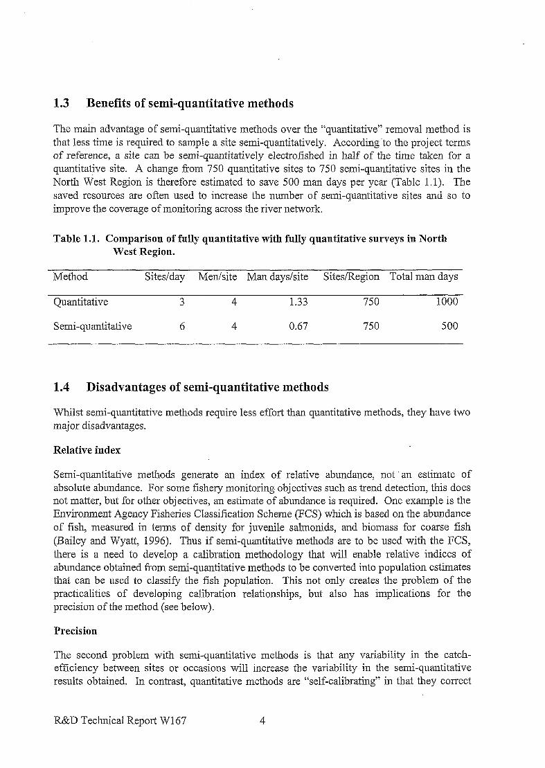
The main advantage of semi-quantitative methods over the “quantitative” removal method is that less time is required to sample a site semi-quantitatively. According ‘to the project terms of reference, a site can be semi-quantitatively electrofished in half of the time taken for a quantitative site. A change from 750 quantitative sites to 750 semi-quantitative sites in the North West Region is therefore estimated to save 500 man days per year (Table 1 .l). The saved resources are often used to increase the number of semi-quantitative sites and so to improve the coverage of monitoring across the river network.

Table 1.1. Comparison of fully quantitative with fully quantitative surveys in North West Region.

Method Sites/day Men/site Man days/site Sites/Region Total man days

Quantitative 3 4 1.33 750 1000

Semi-quantitative 6 4 0.67 750 500

1.4 Disadvantages of semi-quantitative methods

Whilst semi-quantitative methods require less effort than quantitative methods, they have two major disadvantages.

Relative index

Semi-quantitative methods generate an index of relative abundance, not. an estimate of absolute abundance. For some fishery monitoring objectives such as trend detection, this does not matter, but for other objectives, an estimate of abundance is required. One example is the Environment Agency Fisheries Classification Scheme (FCS) which is based on the abundance of fish, measured in terms of density for juvenile salmonids, and biomass for coarse fish (Bailey and Wyatt, 1996). Thus if semi-quantitative methods are to be used with the FCS, there is a need to develop a calibration methodology that will enable relative indices of abundance obtained from semi-quantitative methods to be converted into population estimates that can be used to classify the fish population. This not only creates the problem of the practicalities of developing calibration relationships, but also has implications for the precision of the method (see below).

Precision

The second problem with semi-quantitative methods is that any variability in the catch- efficiency between sites or occasions will increase the variability in the semi-quantitative results obtained. In contrast, quantitative methods are “self-calibrating” in that they correct

R&D Technical Report W167 4

for the catch-efficiency experienced at each site on each occasion, and therefore greatly reduce this. source of variability. The implication of this is that when semi-quantitative methods are used to monitor changes (either spatially. or temporally) in fish stocks, they.. will have. a considerably reduced power compared to quantitative surveys. Thus a decline in fish stocks,, for example, will have to be more severe ,before, a semi-quantitative survey will be able to detect it. One way to compensate-for the reduced precision of semi-quantitative methods is to survey an increased number of sites (for spatial trend detection) or occasions (for temporal trend detection).

There is a danger that the lower cost of semi-quantitative methods will be confused with % increased cost-effectiveness. Whilst the cost of semi-quantitative methods is undeniably less, so is the effectiveness. The cost-effectiveness of semi-quantitative methods --for different Agency monitoring objectives needs to be formally assessed.

1.5 Project Objectives

1.5.1’ Overall Project Objectives

To evaluate the use of semi-quantitative electric fishing and netting results for use in the Fisheries Classification Scheme.

1.5.2 Specific objectives

1. To. review published and..unpublished .literature on the relationship between..data from semi-quantitative methods and fish density for use in the Fisheries Classification Scheme

WV*

2.‘ Where possible: establish useable calibration relationships including appropriate habitat features. This will include the.use of HABSCORE and FCS databases held by WRc.

3, Identify information needs, recommend a program of work to provide this information and, if necessary, produce a costed project proposal.

R&D Technical Report W167

2. POSSIBLE-APPROACHES -TO CALIBRATING SEMI- QUANTITATIVE METHODS

2.1 Introdtiction

Where estimates of abundance are:required -from semi-quantitative methods;it is-necessary to calibrate the methodology.- This involves estimating the catch-efficiency of the method to allow the catch of fish to be multiplied up to a population estimate.

The section starts by describing .the factors that can affect catch-efficiency, and that will therefore .need to be taken into account in a calibration exercise (Section 2.2). There are a variety. of ways of calibrating semi-quantitative methods, and -whilst in practice a mixture of approaches may be used, .the remainder of. this section simply classifies them into:,,

l Spatial calibration (Section 2.3)

l Temporal calibration (Section 2:4)

l Predictive calibration (Section.2.5)

2.2 Factors affecting -catch efficiency

2.2.1 Introduction I

There have been many studies investigating the factors that affect the efficiency of fishing methodologies (Zalewski and Cowx, 1990). However, the majority of these have had the objective of improving the .methodology itself, rather .than .quantifying the influence of extraneous factors with a view to calibrating semi-quantitative approaches. Some- of the primary factors affecting catch-efficiency are described below.

2.2.2 Environmental factors

Catch-efficiency will vary with -environmental -factors, and this is particularly ,~true -for electrofishing (Randall; 1990). Consider .a number of sites’ down a river that are. repeatedly fished as part of a rolling programme.- Habitat-differences such as depth; width, substrate and flow types will result in some electrofishing sites always being more- difficult to fish than others. Similarly, catch-efficiency at all sites will vary between occasions-with changes in. temperature, flow and. turbidity.:- Finally, particular combinations of flow ‘conditions and. habitat will generate apparently random variations in catch-efficiency. These three types. of variation are termed spatial, temporal and random variations respectively.

R&D Technical Report W 167 I

2.2.3 Species and size of fish

Catch-efficiency will vary between species of fish and size of individual fish. In general, larger fish will be more affected by a potential difference in the water column than smaller fish. The behaviour of different species will also affect how readily caught they are, such as whether they reside in sediment (eg eels), under boulders (eg juvenile salmonids), whether they are a shoaling species, or solitary.

2.2.4 Methodology

Changes in fishing methodology will affect the catch-efficiency. Factors include the use of electrofishing or netting, type of electrofishing gear (eg ac or dc), number of anodes, direction of removal (upstream or downstream) and the level of experience of the staff.

One important factor that will determine catch-efficiency is the presence or absence of stop- nets. The removal and mark-recapture methods assume a closed population, and stop-nets are used to achieve this. For semi-quantitative methods, however, stop-nets are generally not employed, and this will permit the movement of fish in and out of the site. The overall effect is likely to be a reduced efficiency when fishing without stops nets compared to fishing with nets, but the magnitude of the effect is likely to be dependent on the habitat and species present.

2.2.5 Successive depletions

As a section of river is repeatedly fished to obtain a removal estimate, the capture efficiency declines (Bohlin and Cowx, 1990). This occurs for a number of reasons. For example, fish which are most vulnerable .as a result of where they are in the reach will tend to be caught first, leaving the less vulnerable fish for subsequent removals. In addition, fish which have not fully recovered from being stunned may be less readily caught on a subsequent attempt. Most methods for obtaining population estimates assume that catch-efficiency remains constant between removals, and the violation of this assumption will tend to produce underestimates of the population size. The implications for semi-quantitative methods is that the catch-efficiency on a single removal will tend to be higher than the average catch-efficiency for the removal method.

2.3 Spatial calibration

To adopt a spatial approach to calibration, for each river survey, the majority of sites can be semi-quantitative, but a few sites must be undertaken using the removal method. The quantitative sites are selected so that all major habitat types are represented and are used to calibrate the semi-quantitative’sites within the same habitat type. Temporal variability in catch-efficiency is therefore controlled by re-estimating the catch-efficiency under the river conditions in which the semi-quantitative sites were surveyed. The method is therefore particularly useful where changes in river conditions (flow, temperature, visibility) between fishing occasion are believed to be a dominant source of variability in catch-efficiency. Spatial variation in catch-efficiency is controlled by habitat stratification.


2.4 Temporal calibration

This is similar to spatial .calibration; however, with this approach, each site in a fisheries survey will have been quantitatively fished at some point in the past. The quantitative data are then used to estimate .the catch-efficiency for subsequent semi-quantitative surveys. Spatial variability is therefore controlled by obtaining estimates of catch efficiency for every site used in the monitoring programme.,. It is therefore particularly useful when spatial factors (habitat, different survey methods) are -believed to be. a dominant. source of variability in catch- efficiency. .Temporal variation in catch-efficiency can only be controlled by trying to sample sites under.similar environmental (flow; temperature) conditions each year.

2.5. Predictive calibration

With this approach, a predictive relationship. is established between catch-efficiency and relevant factors such .as the species and. size of.-fish,. sampling methods used, and .physical features such -as river type:or habitat type. The method is applied .by measuring these predictive factors at the time the semi-quantitative site. is fished, estimating the catch- efficiency from the predictive relationship,- ,and. using this to convert the semi-quantitative catch into a population estimate.

This project is primarily concerned with ‘: the establishment of. .“useable. calibration relationships including appropriate habitat .features”, and the remainder. of this report will. focus on this approach. However,. it must be remembered that for many fishery monitoring. objectives such as trend detection, semi-quantitative methods do not require calibration (Section 1.4), and that when they do, alternative methods exist.(Section 2.2 and 2.4).

R&D .Technical ReportW167 8

3. AGENCY CALIBRATION EXERCISES

3.1 Introduction

There have been three experimental studies undertaken within the Agency. and its predecessors-. to establish the relationship between the catch .from catch-per-area semi-quantitative electrofishing; and the abundance of fish present., All three were concerned with, sampling juvenile salmonids. These were undertaken-in Welsh Region in .1986-1987. (Strange et al, 1989); North West Region in 1992 (Farooqui and Aprahamian, 1993), and in South Westem- Region in 1995 .: (Bird5 1997). All three methods‘ used an experimental approach for developing the calibration relationship;and this is described below.

3.2 Field methodology

The need for an experimental field methodology appears.to be primarily driven by the need to compare -a semi-quantitative method that :does not use stop nets with a population estimate from a methodology that does. The experimental methodology. employed on all three studies was similar; andconsisted, of netting off a section of river (say 5Om), and undertaking a semi- quantitative exercise within a central 30m section. .-The number. of fish remaining in the full 50m section- is then estimated using .standard removal methodology. The efficiency of the semi-quantitative method is assessed by comparing the catch (per area of the 30m length) with the population estimate-(per area of the 50m~length): Whilst this method has allowed for any,.- reduction in efficiency caused by escape of fish from the 30m length, a new problem has been introduced. Given the highly clumped nature of salmonid-populations, the-population density of the 30m section .may be different to the population density of the 50m section.. One effect of this can be seen at low densities, where some single catch estimates are greater than the- quantitative estimates! For example 11% of sites in the south west calibration exercise.(Bird, 1997) gave single-catch estimates of density: for. >O+ trout greater than the quantitative estimates.

3.3 Data editing.

Allthree studies employed some-form of data editing. Bird (1997) did not include. sites at which no fish. were caught during the semi,quantitative method. The reason for this. is unclear, and no guidance is given on how to treat zero catches when applying the method.

Strange et al (1989) and Farooqui and Aprahamian (1993) excluded sites .where the capture efficiency was less than 0.3; The justification given. is that under such circumstances, population estimates are unreliable., Whilst this is true, the removal of sites with low-capture efficiencies is hardly justifiable when the purpose of the exercise is to establish the average capture efficiency and hence the relationship between. semi-quantitative method and-: populations size.

R&D .Technical Report W167 9 ‘-

3.4 Modelling approach

The approach used to derive the calibration relationship was again similar between the three investigations. This involves the use of regression analysis to model the relationship between the semi-quantitative catch per unit area (c/a), and the estimated population size per unit area (n/a). All three investigations produced separate relationships for O+ and >O+ salmon and trout.

The methods differed in a munber of respects, for example

l Bird (1997) and Strange et nl (1989) included a constant term in the model, whereas Farooqui and Aprahamian (1993) did not.

l Bird (1997) considered only a logarithmic model, whereas Strange et al (1989) Farooqui and Aprahamian (1993) considered models on both the natural and logarithmic scale.

l Bird (1997) and Strange et al (1989) considered the population estimate to be the dependent variable, whereas Farooqui and Aprahamian (1993) considered the semi- quantitative estimate to be the dependent variable

Whilst regression analysis provides an approximate approach for developing the calibration relationship, a number of the assumptions required for regression are not met:

l The raw data are counts (c and n) and methods for analysing such data are readily available. The method used in all three approaches, however, was to divide the counts by the area (a) of the site, and treat the resulting ratios as a continuous variable.

l The presence of zeros in the data contradict the assumptions of continuous variables and Normal error structure required for regression techniques. Attempts to resolve this include removing zeros from the data set (Bird, 1997), and by adding 1 to the ratios c/a and n/a (Bird, 1997, Strange et al, 1989, and Farooqui and Aprahamian, 1993).

l For models that regard catch as the dependent variable (Farooqui and Aprahamian, 1993), the dependent variable (c/a) is constrained between 0 and n/a. For models that regard population size as the dependent variable (Bird, 1997, and Strange et al, 1989), the dependent variable (n/a) must be greater than the catch (c/a). For both models, the residual variance will increase with increasing values of the independent variable. Regression assumptions of Normality and homoscedasticity (constant variance) are unlikely to both be met, even after transformation. For example, residual analysis for log(n/a+l) (Bird, 1997) shows a positive skew to the residuals and decreasing variance at high catches.

It must also be remembered that population estimates obtained from the removal method are themselves biased, sometimes considerably so. This is true even when all of the assumptions of the removal method are met! This bias will be reflected in the calibration relationships derived from them.


3.5 Results obtained

The performances of the calibration exercises were measured by I? values and classification.. : ! errors- (Table 3.1). High I? values. are obtained. for all studies, particularly for 0; fish where higher densities are encountered. Classification. errors are probably :the more. meaningful measure of performance in that they reflect the application for which the models will be used. Classification-errors vary between 10% and 36%.

Table 3.1. Performance of calibration models

I? (nat/log) 0+ salmon

Bird (1997) Strange et.al. (1989)

- 196.8 85.1 186.4

Farooqui & Aprahamian (1993).

96.1.i 89.0 >O+ salmon -195.7 78.3 178.5 85.1 190.0 o+ trout - 192.4 89.2 190.2.-. 93.6 195.2 >o+ trout - I 86.3 51.5 168.8 83.4 186.3

Classification assessed

National FCS (F-class omitted)

Welsh classification Welsh classification

Classification O+ salmon 17.0 9.7 22.2 error (%) >O+ salmon 20.5 29.4 30.0

o+ trout 21.2 16.0 10.5 >o+ trout 35.8 34.6 28.2

Bird (1997) concludes “the overall- distributions of quantitative and single catch grades were,- nevertheless, similar in all cases with no clear tendency for single catches to over. or underestimate grades. In the context of catchment- overview of stock status this level of accuracy is perfectly acceptable”

3.6 Refinementsrequired:

All three methods have successfully produced calibration relationships that. can be used to convert semi-quantitative catches .into population estimates. However, there are. a number of ways in which the approaches can be further refined.

1. Correction. for, different fishing -conditions. The use of regression is very similar-.-in practice to simply assuming that the particular species/age class of fish has a constant probability of capture at all sites.. For example, the regression relationship for trout parr:. derived by Bird .(1997) is very similar to assuming a constant catch efficiency of 0.62,;


Thus a catch of 8 fish, for example, would generate a population estimate of 13 ( = 8 / 0.62). The assumption of constant catch efficiency for all sites, regardless of width, depth, habitat, flow conditions and fishing methods (e.g. number of anodes) is clearly unrealistic. A useful extension would therefore be to produce a methodology that adjusts the calibration relationship for different river types or fishing’methods. A specific objective of this project is “where possible, establish useable calibration relationships including appropriate habitat features”

2. Uncertainty associated with calibration. Catch-efficiency varies considerably both spatially and temporally, and there will therefore be large uncertainty associated with assessing abundance from semi-quantitative methods. However, none of these calibration studies provided a method for estimating the uncertainty associated with the population estimate. In the context of the KS, this involves assessing the probability that a designated class is correct.

3. Statistical methodology. Given that the raw data are counts of fish, the statistical methodologies could be refined to properly allow for this.

The next section outlines a modified calibration methodology that addresses these three areas.


4. DEVELOPMENT OF A NEW CALIBRATION ’ METHODOLOGY

4.1 Introduction

In this section, the development of a new statistical calibration methodology is.described. The methodology. could -be used to develop calibration relationships from ,any source of data, such : as thosecollected for previous Agency calibration exercises (Section 3). For the purpose of this report;- the method is illustrated using .data from .a quantitative electrofishing survey of trout parr populations at arotmd .600 sites in England and Wales. For each site, data were available for. the population estimate from the removal method (n), the catch of fish from the first removal (c) and the area of.the site .(a), .together with numerous map- and site-based habitat variables. The catch (c) from the first removal, together with habitat information, .will be used to-predict the population size (n).

It must be stressed that the context for the application of this calibration methodology is to enable a cheaper, low precision method at sites where quantitative ,methods would be possible if resources allowed. Such calibration exercises cannot be extrapolated to situations where semi-quantitative methods are being deployed because quantitative estimates are not possible (e.g. some lowland~rivers).

This section starts by describing the revised statistical assumptions made for this calibration methodology (Section 4.2):. The way- that a correction for fishing conditions (e.g. habitat) can be built in to the methodolo,T is described in Section 4.3, and-the estimation of population size-is described in Section 4.4. The final section (4.5) describes a number of approaches for assessing the -uncertainty associated with using’semi-quantitative methodsfor assessing fish abundance and FCS class.


4.2 Improved statistical basis ~

The relationship between the catch, population size and FCS class for the sites on the database is shown in Figure 4.1. Previous calibration exercises have used a regression approach to relate the semi-quantitative catch (c) to the population size (n). Transformations of the data were used to try to achieve the assumptions of regression such as constant variance and Normality. Consideration of the way the data are generated leads to a more natural model which assumes that the catches (c) obtained from a semi-quantitative method with constant catch-efficiency (p) from a large number of sites with the same population size (n) would follow a Binomial distribution (Appendix A). In practice, the efficiency of the method will vary from site to site, and therefore the catches obtained from sites with the same population size will be more variable than expected from the Binomial distribution. This is known as an “over-dispersed” Binomial distribution. The use of such distributions is also the basis of recent developments in mark-recapture methods (Bayley, 1993) and removal methods (Wang, 1996).

40 50 60 70 60 90 100

Population size (n)

Figure 4.1. Relationship between catch, population size and FCS for trout Parr. Diagonal line denotes a catch equal to the population size. Populations ~100 not shown for clarity.


4.3 Correction-forfishing conditions

Some of the variation in catch-efficiency between sites may be predictable; particularly if it is determined by environmental factors. such as the conductivity.of the water, river depth and-. width. The estimate of the population size (n)- from a particular catch of fish (c). will therefore vary between different river types. The simplest way to do this is to model the relationship between river type and catch-efficiency, and stillused the Binomial;,model described in Section 4.2.

This is achieved in practice by fitting: ~a model- of. catch. against- population size : and environmental variables, using an over-dispersed .Binomial model (McCullagh and, Nelder, 1989; Williams,. 1982). For demonstration purposes, a model relating the catch-efficiency for >O+ trout to width, depth and conductivity has been developed (Appendix B). Population size is itself estimated from the removal -method;..and so the modelling procedure used here is-. approximate.

From -the- resulting model, we can estimate the average catch-efficiency Q+,) for a particular. river type, and in addition obtain an estimate of the degree to which the catch-efficiency varies about this mean from site to site (over-dispersion parameter, 4). For example; consider a site 5m wide,: with an average depth of 20cm, and a conductivity of [email protected]‘. The catch- efficiency model for >O+-trout estimates the average catch efficiency &,) to be 0.69, and the overdispersion parameter (4) to be 0.07 (Appendix C). Sites that are.wider, deeper or with a lower conductivity would have a lower catch-efficiency. For example, if the.site has -a width of 1Om;’ depth ‘of 40cm -and -a conductivity of [email protected]‘, the model predicts a catch- efficiency of 0.45.


4.4 Estimating population size from semi-quantitative catch

To estimate the population size, we need to specify more precisely the form of the overdispersed Binomial distribution. A commonly used model is the Beta-Binomial which assumes that values of p are distributed according to a Beta distribution, and that for a given p, the catches are distributed according to a Binomial distribution (Appendix A).

To illustrate the methodology, consider the site described in Section 4.3, with the additional information that eight fish are caught (c=8) and the area (a) is 23Om’. From this information, we need to obtain an estimate for the population size (n). From the Beta-Binomial model (with pr, .= 0.69 and $ = 0.07) we can calculate the distribution of possible catches that could be obtained from different population sizes. The distributions of possible catches for population sizes nine, ten and eleven are shown in Figure 4.2. Thus, for example, if the population size is ten, the catch obtained from the semi-quantitative method cannot be greater than ten, is most likely to be around seven or eight, and very unlikely to be as low as zero.

0.25 T

I jl&l=9 1

I

0.20 I

j

~ 0.15

E 2 P

4 0.10 T T

I 0.05 +

!

I ‘; 0.00 .

Ian=101

c 0 1 2 3 4 5 6 7 8 9 10 11 12

Catch (c)

Figure 4.2. Distribution of possible catches for population sizes of nine, ten and eleven given a catch-efficiency of 0.69. A Beta-Binomial model is assumed.


The calculations used to produce. the histograms shown in Figure 4.2. can also -give the probability of catching eight fish fYr0m.a wide range of possible population sizes (from eight to very large). The probability of observing a particular-catch for different population sizes is termed the “likelihood” of catch (Figure 4.3). .Thus the likelihood of catching eight fish given.’ a population of nine, -ten and eleven is 0.18, 0.20 and 0.19 respectively. This example is shown in both Figure 4.2.(Catch = 8) and Figure 4.3 (Population size =‘9, 10 and 1.1):: A common type of estimate in statistical inference is the “maximum likelihood estimate”; in this- context, this would be the population size that gives the maximum likelihood of observing the catch. From Figure.4.3, it can be seen that for a catch of eight fish, the maximum.likelihood estimate for the population size is ten. .- This- can then. be expressed as a density or biomass (if weight information available) as reqnired. For example, the maximum likelihood estimate for the density:is 10/230x100 = 4.3 loom-‘.

The frequency distributions of catches for different, population- sizes (Figure .4.2): and : the likelihood function (Figure 4.3) are used here to illustrate the rationale. :behind the methodology. In practice, a simple equation is used to estimate the population size from a catch (Appendix D). This equation is a special case of the Maximum Weighted Likelihood estimator for the removal method (Carle and Strub, 1978) for the case of a single removal.

Figure 4.3. Likelihood of obtaining a catch of eight fish given different population sizes, given a catch-efficiency-of 0.69. The maximum likelihood-estimate of the,. population size is ten. .:


4.5 Estimating the uncertainty associated with calibration

4.5.1 Introduction

Having obtained an estimate of the population size, it is necessary to assess the precision of the estimate. This particularly important in this context where the use of a calibration relationship is likely to render the resulting estimate far less precise than would have been obtained from the removal method (Wyatt and Lacey, 1994). Three measures of uncertainty are described here: variance (Section 4.5.2), confidence intervals (Section 4.5.3), and most importantly in the context of the FCS, “probability of class” (Section 4.5.4).

The methods presented here will underestimate the variance associated with semi-quantitative methods. This is because whilst it allows for the degree to which catch-efficiency will vary from site to site (measured by overdispersion parameter ($j), Section 4.3) it ignores the uncertainty associated with estimating the underlying mean (pP,, Section 4.3). This needs further consideration before the method is used operationally (see Section 6.3.2).


4.52 Variance

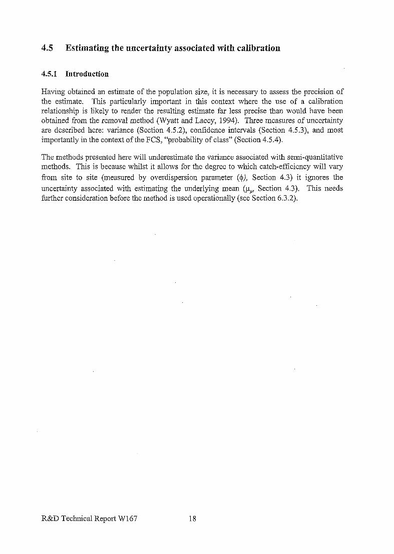
The variance of the population estimate can be thought of as the variance of the population estimates that would be obtained from the repeated fishing .of a site with a true population of ten fish. This in turn is calculated from the distribution of catches.that would be obtained from a population of ten fish, using the Beta-Binomial distribution; From Figure 4.2’it can be seen, for example, that there is a 7% chance of catching all ten fish. A catch of ten fish would give a population *estimate of .13 fish (from. Appendix .D).-...,The distribution of possible population estimates from a population of ten fish is shown in Figure 4.4. There are 11 columns corresponding to catches from. 0 to 10 fish. The variance of this distribution is the sampling variance, and is found to be 6.32 (Appendix D).

0 T- N m d ul ccl r- 03 a 0 (v m e Lo Y z 7 r-7 r

Estimated population size

Figure 4.4. Frequency.distribution of estimates of populatidn size when the true !_ population size is 10 fish; and the,catch efficiency is.O.69.

R&D .Technical ReportW167- 19

4.5.3 Confidence intervals

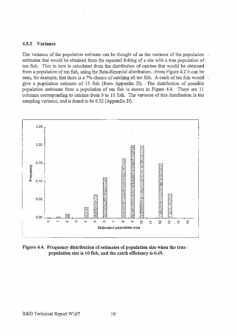
Confidence intervals can be estimated directly from the frequency distributions of catches for different population sizes. To estimate an upper 95% confidence limit, we need the population size for which there is I 2.5% chance of obtaining less than or equal to the observed catch of 8 fish. This gives an upper confidence interval of 24 fish (Figure 4.5). Similarly the lower 95% confidence interval is found to be eight fish. Whilst the probability of catching eight fish from a population of eight is greater than 2.5%, a catch of eight fish is impossible from a smaller population.

As with the removal method, the confidence intervals for the population estimate cannot be estimated from the sampling variance (unless the population size is large, and the data can be assumed to follow a Normal distribution). For example, a catch of zero fish at this site will give a population estimate of zero, and the variance of this estimate will also be zero. This is because repeated sampling from a site with a true population size of zero will always give the same population estimate (zero!). The upper confidence limit of this zero estimate, however, will be four. This reflects the fact that a zero catch could arise by chance from a small population size.

0.25 T

I ! 0.20 {

1 I

0.i5 I

6 5 z 2 I LL 0.10 f

]

jo j q n=24 !

Figure 4.5. Frequency distribution of catches for populations sizes of n=8 and n=24. Catch efficiency is 0.69.


4.54 Probability of Class

Introduction

The primary objective of this report is to~discuss.links between semi-quantitative methdds’.and the Fisheries Classification Scheme (FCS). -Perhaps the most useful.measure of the precision of a population estimate in the context of the FCS is what.this report will-term YProbability of Class”. This is .the probability(chance) that the true (but unknown) population at a sampling site falls within each of the FCS classes (A to F).’ It is perhaps surprising that this is not calculated from the density estimate, variance or confidence intervals discussed above.

From Figure 4.1 it can be seen that a particular catch may. arise from ,a number of different I classes. For example, a catch of eight fish cannot have arise fr0rn.a class F or E, is most likely to have arise from a class D or C, and there is even a chance that it was from a class .B. Similarly, a catch of 30 fish cannot have arisen from a class F, E, D or C site; is most likely to have arise from a class B.-site, but.may have-arisen from a class A. The probability of each class can then be used to obtain the most probable class. In some cases, the class that corresponds to the population estimate-willnot be the same as the most probable class!

The method .by- which Probability of Class is calculated arises from a branch of statistical inference known as Bayesian statistics (see Gelman et al, 1995 and Carlin and Luois,- 1996, for . recent overviews). In Bayesian statistics, the starting point for making inferences from data is the .prior belief, described by a “prior distribution”, about the unknown parameter.. In this context, this is our prior belief about the.likely population size, before we sample the site. The catch obtained by the semi-quantitative survey method is then used to modify the prior distribution to give a “posterior distribution” that reflects the frequency distribution.: of, possible population sizes, and thus fishery classes.

R&D. Technical Report W 167 21

Prior expectation of fish densities

Before semi-quantitative sampling is undertaken, it is possible to say something about our expectation of the density of fish in the site. For example, if the new site is regarded as being from the same “population” of sites from which the calibration data were obtained, we can use the frequency distribution of densities in the calibration data set to give our prior belief about a site.

The, average density of >O+ trout in the calibration data was 18/100m2, and 12% of sites had no fish present. The frequency distribution for numbers of fish per 1 OOm’ is shown in Figure 4.6, and this has been modelled by a Negative Binomial distribution (Appendix E).

0.18 T

0.16 I

2 0.1

5 ii g 0.08

LL

0.06

observed

-expected

Number of>O+trout

Figure 4.6. Distribution of numbers of >O+ trout (per 1OOm’) in England and Wales. Expected frequencies are obtained from a Negative Binomial distribution.


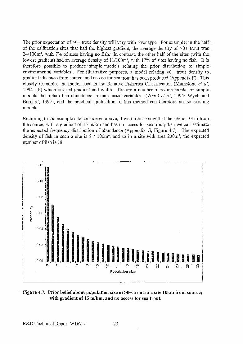
The prior expectation of >O+,trout density will vary with river type. For example; in the half. I of the calibration sites that had the highest gradient, the average density of >O-i- trout was 24/1OOm’, with 7% of sites having no fish:: In contrast, the.other half of the sites (with the lowest gradient) had an average.density of ll/lOOm’, with 17% of sites having no fish. It is therefore possible, to produce simple -models .relating the prior distribution to simple. environmental variables. For illustrative purposes, a model relating >O+ trout density to gradient,; distance from source, and access. for sea trout has been produced (Appendix F). This closely resembles the model used in the Relative Fisheries Classification (Mainstone et al, 1994 a,b) which utilised gradient and width. The. are a number of requirements- for simple. models that relate fish abundance to map-based variables (Wyatt -et al, 1995; Wyatt and Barnard, 1997), and the practical application of this method can therefore utilise existing models.

Returning to the example site considered above, if we further know that the site is 1Okm from the source, with a gradient of 15 m/km and,.has no access for sea trout;- then we can estimate the expected frequency distribution of abundance (Appendix G, Figure 4.7). The expected density of fish in such a site is 8 / 100m2, and,so in a. site with area 230m2, the .expected number of fish is 18.

Figure 4.7. Prior belief about population size of >O+. troutin a site 1Okm from source; with gradient of 15 m/km, and noxaccess for sea trout.

R&D:Technical Report W167. 23

Calculating the posterior probability distribution

The posterior probability distribution is estimated from the likelihood of the data (Section 4.4, Figure 4.3) and the prior probability of that population size (Figure 4.7), using Bayes theorem (Appendix H) :

Posterior . . . is proportional to . . . distribution

more specifically:

Likelihood function

X Prior distribution

Probability of Likelihood of Probability of population n . . . is proportional to . . . catch c given x population n given catch c population n

These calculations can be readily implemented using a spreadsheet (Appendix I). The posterior distribution for the example of a catch of eight fish is shown in Figure 4.8. In this example, the posterior distribution closely resembles the likelihood function (Figure 4.3), illustrating that the prior distribution (Figure 4.7) has a low degree of influence.

0.16

0.14

0.12

0.10

0.04

0.02

0.00

T

-L

: : :

Figure 4.8. Posterior probability distribution for >O+ trout population size, given a catch of eight fish.


The posterior distribution can be.used to derive.whatever summary statistics are required, such as the mode, median or mean: However, the discussion here will be limited.to the assessment . of probability of class. Converting population size:to density and FCS class (Appendix I), we see that the most likely class is a D (Figure 4.9). In addition, we see that -there is a 46% chance that the site was a C, and a 1% chance that the site was a B. Thus overall -there ,is a. 47% chance that the site has been mis-classified.

D C B. A

Class

Figure 4.9: Probability:of class for a cat&of 8.>0+ trout from a site,of area 230m’.

The probability ofclass will alter- for different catches and river conditions. For example, Table 4.1 shows the probability of class ,for the site described above for a range of catches from 0 to. 10. In contrast, Table’,4.2 gives the same.information.for a larger site..with a lower conductivity. The classification- for a given catch is higher and less certain for the larger site,. reflecting the lower catch efficiency.


Table 4.1. Probability of class for semi-quantitative catches between 0 and 10 trout parr in a river of width 5m, conductivity [email protected]’ and depth 20 cm. Boxes denote most probable class.

Catch Class F E D C B A

0 1, 79 21 1 96 4 2 83 17 3 57 42 1 4 23 73 4 5 91 9 6 83 17 7 70 30 8 53 46 1 9 35 64 1

10 17 81 2

Table 4.2. Probability of class for semi-quantitative catches between 0 and 10 trout parr in a river of width 15m, conductivity [email protected]’ and depth 50 cm. Boxes denote most probable class.

Catch F E

Class D C B A

0 40 42 14 4 1 44 37 16 2 2 17 45 31 6 1 3 5 .39 44 10 2 4 1 27 53 16 3 5 16 57 22 6 6 8 55 28 9 7 3 51 34 12 8 -1 44 40 15 9 36 44 19

10 29 47 24


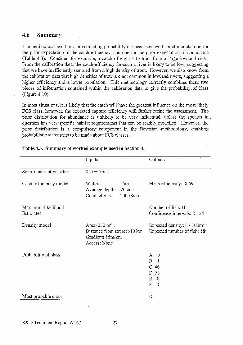
4.6 Summary.

The method outlined here for estimating probability of class uses two habitat models;.one for the prior expectation.of the catch efficiency, and one for the prior expectation of abundance (Table 4.3). .Consider,.for example, a catch of eight SO+ trout :from a large lowland river. From the calibration data, the catch-efficiency for such a river is likely to be low, suggesting that we have-inefficiently sampled from a high density of trout.-- However, we also lurow from. the calibration data that high densities of trout are not common in lowland rivers,. suggesting a higher efficiency- and a lower population. This methodology correctly combines these two pieces of information contained within the calibration data to give the probability. of class (F&we 4.10).

In most situations, it is likely that the catch will have the greatest influence-on the most likely FCS class, however, the expected capture efficiency will further refine the assessment. The prior distribution for ‘abundance,- is unlikely to be very influential,, unless the species in question has very specific .habitat requirements that can be readily .modelled. However, the prior distribution is a compulsory component in the Bayesian -methodology, enabling probabilistic statements to be made about FCS classes.

Table. 4.3. Summary of worked ‘example used in Section 4.

Inputs outputs <.

Semi-quantitative catch 8 >O-i- trout.

Catch-efficiency model. Width: 5m Average depth: .20cm Conductivity: 200jLYcm

Maximum likelihood Estimates

Density model,

Probability-of class

Most probable class

Area: 230 m2- . . Distance from source:- 10 km Gradient: 1 S&km Access: None

Mean efficiency:. 0.69

Number of fish: 10 Confidence-intervals: 8 - 24

Expected density: 8 / 100m’ Expected number of fish: 18

A 0 B 1 C 46 D 53 E 0 F 0

D


Fisheries Classification Scheme class

t Posterior distibution for

I number of fish at site I

Prior distribution for

Catch-efficiency Model

f

Prior distribution for number of fish at site t-

&

Figure 4.10. Summary of approach for obtaining the PCS class from a semi quantitative method.


5. DATA REQUIREMENTS FOR.CALIBRATION

5.1 Introduction . .

Having established the methodology for calibrating semiLquantitative methodologies, it is now possible to determine the data requirements (Section-5.2) and,,data sources (Section 5.3) for- further- calibration exercises for a range of target species.

5.2 Type:of data required.

To adopt the methods outlined in Section 4,.the following data,are required:

Fishery information (for each species / age class)

l Population estimate (preferably obtained fkomunbiased methods) l Catch obtained from semi-quantitative methodology

Information relating to expected catchability

l Type of sampling (netting, electrofishing) l River characteristics (eg width and depth) _‘- l Environmental factors affecting efficiency of method (eg conductivity for electrofishing) l ,Methodology (eg number of anodes for electrofishing)~

Information .reiating.to expected. abundance (for.Probability of Class - optional)

l Map-based variables (eg gradient, distance from source, access for adults) l Field-based variables (eg substrate, cover)

5.3 Potential-data sources

The calibration methodology outlined in this report can be implemented using two types of r data:-

1. Data collected specifically for ,the exercise:using the experimental approach similar to that outlined in Section.3; or

2. Routine quantitative survey data collected for fishery management purposes as used in Section 4.

The advantage of the experimental approach is that factors such as the influence of stop nets can be directly assessed. However, the approaches used to.date-introduce additional problems due to the differences in fish density between the shorter semi-quantitative site and the longer quantitative site. The advantage of using routine quantitative survey data is that ,potentially

R&D Technical Report, W 167 29 :

large quantities of data can be accessed fi-om regional and national archives, however, certain approximations may need to be made regarding the relationship between the first run of a removal method, and the semi-quantitative catch.

Existing regional databases include Fins (used by a number of Regions), SurvForm (Southern), and FDPS (Anglian). In addition, a flexible database system has been developed by Midlands Region, and is being considered as a “Best Interim Solution” (BIS) for national implementation. However, this has not yet been implemented and therefore does not currently provide a useable source of data. National databases collected for R&D projects include HABSCORE and the Fisheries Classification Scheme. A summary of regional and national databases is given Table 5.1.

Table 5.1. Summary of data archived on Agency database systems.

Fins SurvForm BIS FDPS HABSCORE FCS

General Regions

National collation

Fishery data Population estimate

Catch from first removal

Habitat data Field-based habitat measurements

Methodology

Map-based habitat measurements

Details of methodology

NE, SW, S: T

NO

Yes

No

Option

NO

NO

S M A

No Proposed No

Yes

Yes

Yes

Yes

Yes

Yes

No Option No

No Option No

No Option No

Yes

Yes

No

Yes

Yes

No

Yes NO

Yes Gradient

No No

It can be seen that one problem with many existing data sources is the lack of objective information on factors that will influence catch efficiency such as habitat and fishing methodology. In addition, to use the statistical methodolo,T outlined in Section 4, the catch recorded on the first removal is required, and a number of systems do not archive this information.


6. RECOMMENDATIONS FOR FURTHER WORK

6.1 Introduction

This report reviews some.of the issues associated with attempting to classify fisheries based on semi-quantitative methods. In addition, a .new methodology has been described for calibrating semi-quantitative methods, and this has been illustrated by developing a calibration relationship for >O+ trout.

However, there remain a number of unresolved issues relating to the use of semi-quantitative methods for fisheries management within the Agency, and areas where further development is required.

Recommendations are given here for:

Change in operational practice:

l Routine collection of data relating to capture efficiency (Section 6.2.1)

l Collation of a national database (Section 6.2.2)

l Development of calibration relationships (Section 6.2.3)

l Development-of implementation software (Section 6.2.4)

R&D Needs:

l Assessing alternative approaches to predictive calibration (Section 6.3.2).

l Assessing the cost-effectiveness of semi-quantitative methods (Section 6.3.1)

l Assessing alternative approaches to predictive calibration

l As has been noted throughout- this report, semi-quantitative methods can be used without the need for calibration,- such as for. trend detection. However, some objectives will. require the conversion of semi-quantitative data into population estimates. The use of predictive calibration relationships based on habitat features. (Section 4) is only one of-a number of possible ways of approaching this problem .(see Section 2). It istherefore recommended that further work is undertaken as part of the R&D programme to assess alternative approaches for calibrating semi-quantitative methods.

l Refinement of the calibration methodology (Section 6.3.3)

l Refinement of quantitative methods (Section 6.3.4)

l Calibration of 5-minute sampling methods (Section 6.3.5)

R&D .Technical Report W I67 31

6.2 Change in operational practice

6.2.1 Routine collection of data relating to capture efficiency

The development of calibration relationships for a range of different species and size is largely constrained by the availability of suitable calibration data. Unfortunately, the availability of suitable routinely collected (quantitative) calibration data is becoming more limited with the increasing adoption of semi-quantitative methods. Furthermore, where quantitative fishery data is collected, there is not any consistent collection of ancillary information relating to catch efficiency. It is therefore recommended that the Agency consistently records information on factors that will affect sampling efficiency on all routine surveys. This will include simple information on the gear and methods used, and the habitat and river conditions. With the proposals to implement a standard fisheries database system, it is suggested that the facilities to record such information are included as standard data entry fields in this system.

6.2.2 Collation of a national database

A national database of consistent information relating to the efficiency of survey methods (Section 6.2.1) will take a number of years to establish. In the meantime, existing databases (Section 5.3) provide the facility for developing calibration relationships to varying levels of sophistication for different species. For juvenile salmonids, calibration relationships similar to that developed for >O+ trout in this report can be developed for 0+ trout and salmon. However, data on methods (e.g. number of anodes) are not available. For coarse fish, there are less quantitative data available due to sampling problems in large lowland rivers,. Even where quantitative data are available, supplementary data on methods and habitat are not cornmon. However, even in the absence of supplementary information, the methodologies outlined in this report can still be used to estimate the average catch-efficiency for a particular species, and the variability associated with the conversion from semi-quantitative data to population estimates.

It is recommended that existing data that are suitable for establishing catch-efficiencies for different species groups are collated on a national basis. However, collation of national data sets is currently being proposed for a number of other R&D projects including coarse fish recruitment and the river fisheries habitat inventory. It is therefore recommended that where feasible, a single collation exercise meeting the requirements of a number of R&D projects is planned.

6.2.3 Development of calibration relationships

Calibration relationships should be developed for the full range of species covered by the Fisheries Classification Scheme. The FCS is based on species groupings (Rheophilic, limophilic etc), and so the calibration relationships should be developed in a way that will permit the classification of a species group (rather than individual species). The calibration


exercise should follow the methodology. developed in this Phase of. the project. Where information on factors influencing catch-efficiency are not available, the same methodology should still be followed, thus addressing the second and third benefits, of the methodology (Section 3.6);.but not the-first.

6.2.4 Development of implementation, software

The calculation of the probability of class from semi-quantitative- data is too complex to be undertaken without the aid of a computer.. Whilst the calculations can be readily programmed into a spreadsheet by individual users, it is clearly more efficient for software to.be developed once nationally.-. The Agency- currently operates a number of software packages .for archiving and analysing survey data, and. .these include an MS Access-based being developed in Midlands Region (to be adopted nationally :as a Best Interim Solution, BIS), the Fisheries Classification-Scheme software and the HABSCORE software. The ultimate aim. is for the functionality of the latter two to be incorporated into the first. The methodology for assessing. probability of class contains elements of all three software programmes: use of habitat models (HABSCORE)~ the use of the FCS (FCS software) and the estimation of abundance from survey data (BIS database).,. If incorporation of probability of.class into the BIS .database is not-possible-in the near future, then development of independent software,.or development of the current FCS software are possible interim solutions.

6.3 R&D Needs

6.3.1 Assessing the:cost-effectiveness of semi-quantitative methods

The widespread adoption of semi-quantitative methods.within the Agency has been driven by the need for cost-effective monitoring .programmes and. the ‘need to assess rivers where quantitative methods-.are not possible. However, the cost-effectiveness of semi:quantitative methods for the range of Agency monitoring objectives has not been established. For many objectives, it is likely that semi-quantitative methods will. provide the most cost-effective option, but this may not be true for all objectives. Is the increased risk of incorrect management decisions associated with semiYquantitative methods too high a penalty to pay for the reduced resource requirements?

It is therefore recommended that a work -programme is developed to assess the cost- effectiveness of semi-quantitative methods. To do this, it will be necessary to clearly identify the reasons why,the Agency undertake monitoring, and how the information is used to manage fisheries. In addition,-it will be necessary to,look at semi-quantitative.methods against the full range of-alternatives, not just quantitative survey. techniques. These will include the analysis of angler catches, traps, counter and acoustic techniques.

Whilst components ‘of such an appraisal may need to be undertaken as part of the R&D programme, many. of the issues will ..be assessed as part of the work programme for the : Agency’.s Fisheries Monitoring Review Group.-; It is anticipated that the work of this group will identify the details of further R&D needs in this area.


6.3.2 Assessing alternative approaches to predictive calibration

As has been noted throughout this report, semi-quantitative methods can be used without the need for calibration, such as for trend detection. However, some objectives will require the conversion of semi-quantitative data into population estimates. The use of predictive calibration relationships based on habitat features (Section 4) is only one of a number of possible ways of approaching this problem (see Section 2). It is therefore recommended that further work is undertaken as part of the R&D programme to assess alternative approaches for calibrating semi-quantitative methods.

6.3.3 Refinement of the calibration methodology

Classification of reach based on several sites

The methodology developed in this report allows the classification of a single electrofishing or netting site. However, there are many circumstances where the classification of a river reach based on sampling at a number of sites is required. This is particularly true for lowland coarse fish species where the shoaling and movement of fish renders the classification of a single site less meaningful than for juvenile salmonids.

There is therefore a need to extend the methodology in this report to the classification of reaches based on several sites. This will introduce a number of additional issues, such as the influence of between-site variability on the Probability of Class for the reach.

Variability in catch-efficiency in space and time

The methodology presented in this report makes no distinction between the variability of catch-efficiency between sampling occasions, and variability between sampling sites. An assessment of the degree of spatial and temporal variability in catch-efficiency for different species and river types will facilitate a refinement to the methodology outlined in Section 4. In addition, it will provide an essential input into the development of reach-based classification (Section 6.2.1), the assessment of the cost-effectiveness of semi-quantitative methods (Section 6.3.1) and assessing the alternatives to predictive calibration (Section 6.3.2).

Improvements to the assessment of uncertainty

The method presented above underestimates the variance associated with semi-quantitative methods. In the context of estimating the variance and confidence intervals, improving this would involve including the variance associated with the mean catch-efficiency given by the habitat model. In the context of estimating the probability of class, it would involve assessing the uncertainty associated with the prior distributions. To do this may be too complicated for the analytical (equation-based) approaches described in this report, and may require the use of Monte-Carlo methods, similar to those used by the Environment Agency for the removal method (Wyatt and Lacey, 1994; Wyatt and Lacey, 1995). Such refinements may not make much difference in practice, but this should still be investigated.


6.3.4 -Refinement of quantitative methods

Probability of class

This report outlines a methodology for assessing: Probability of Class for. semi-quantitative methods. However, no such methodology exists for quantitative sampling methods! There is therefore a need for the development of a consistent approach to assessing Probability of Class for all population estimation methodologies.

Classificatiofi of reaches

It has already been mentioned that there-is a need for the development of a.methodology for determining the probability of class for a reach based on a number. of semi-quantitative sites. Once again, such a methodology does not currently .exist for quantitative methods, and there is a need for consistent methodology development for both quantitative. and semi-quantitative methods:

6.3.5 Calibration of 5-minute sampling methods

Much of the discussion in this report.has related to the,use of semi-quantitative catch per unit area methods. There is a possible requirement..for calibrating catch per-unit time .methods such as five-minute fi-y sampling. This could not be done .with routinely collected survey data, and would therefore require the collection of experimental calibration data from sites where five-minute fry sampling and an independent assessment of fry density are undertaken.

However, five-minute ii-y sampling is most commonly regarded as a provider of-an index of. relative abundance for detecting spatial patterns and. temporal trends, rather than as a cost- effective means .of estimating absolute abundance. The need to convert such indices into. population- estimates and FCS classes has not been demonstrated (Section 6.3.1).


7. REFERENCES

Bailey, S and Wyatt. R.J: (1996). The -Fisheries Classification System.. Presented at the Institute of Fisheries Management 27th.Annual Study Course, York; September, .1996.

Bayley, P.B. (1993) Quasi-likelihood estimation of marked fish. recapture: Can.J.Fish.Aquat.Sci., 50, 2077-2085.

Bird, -D.J. (1997). The use of cost effective single catch electric fishing methods in the routine monitoring of juvenile salmonids. .:Fisheries Technical Report, FRCN/97/0 1:.

Bohlin, T. and Cowx; I.G. (1990): Implicationsof unequal probability of capture by electric fishing on the estimation of population size. -In: Developments in Electric .Fishing. (I.Cowx, ed.). Fishing News Books, Blackwell, Oxford.

Carle, F.L. and Strub, M.R. (1978)’ A new method for estimating population size -from,. removal data. Biometrics; 34, 621-630.

Carlin, B. and Louis, T. (1996): Bayes and Emprical Bayes methods -for data- analysis. Chapman and Hall.

Farooqi, -M.A. and Aprahamian, M.W. (1993). : The calibration of a semi-quantitative approach to fish stock assessment in the North West Region of the NRA: Internal Report.

Gelman, A., Carlin, J., Stem, H. and Rubin, D. (1995); Bayesian data analysis. Chapman and. Hall.

Harding,- C.M., ,Heathwood, A.W., Hunt-;-R.G. and Read, K;Z.Q. (1984) The estimation of animal population size by the removal method, The Journal of the Royal Statistical Society, Series C 33, 196-202.

Mainstone, C.P., Barnard, S. and: :Wyatt, R. (1994a) The NRA National Fisheries Classification Scheme. A guide for users..R&D.Note.206. -.102pp.

Mainstone, C.P., Barnard,. S. and Wyatt, .: R. (1994b). Development of. a Fisheries Classification Scheme. Report to NRA 244/7N. 220~~:

McCullagh. .-P. and Nelder, J.A. (1989). Generalised Linear .Models. Second Edition. Monographs on Statistics and-Applied Probability 37.’ Chapman and Hall. i

Moran, P.A.P (195 1) A mathematical theory of animal trapping, Biometrika 3 8, 307-3 11.. I

Randal1,z.R.G. (1990) Effect of water temperature, depth, conductivity and survey area on the catchability of juvenile .Atlantic salmon by electric fishing in New Brunswick streams. In: Developments in Electric Fishing. (I.Cowx, ed.). Fishing News Books, Blackwell, Oxford.

R&D Technical Report Wl.67‘ 36

Schnute, J. (1983) A new approach to estimating populations by the removal method, Canadian Journal of Fisheries and Aquatic Sciences 40,2153-2169.

Strange, C.D., Aprahamian, M.W. and Winstone, A.J. (1989). Assessment of a semi- quantitative electric fishing sampling technique for juvenile Atlantic salmon Sahno salar L. and trout, Salmo trutta L., in small streams. Aquacultuve and Fisheries Management, 20, 485- 492.

Wang, Y.-G. (1996) An extravariation model for improving confidence intervals of population size estimates from removal data. Can.J.Fish.Aquat.Sci., 53,2533-2539.

Williams, D.A. (1982) Extra-binomial variation in logistic linear models. Appl. Statist., 31, 144-148.

Wyatt, R.J. and Barnard, S. (1997) River Fisheries Habitat Inventory (Phase 1). Scoping Study. Draft R&D Technical Report. Environment Agency. 85pp.

Wyatt, R.J., Barnard, S. and Lacey, R.F. (1995) Salmonid modelling literature review and subsequent development of HABSCORE models. Report to NRA No. 338/20/W; WRc. 189pp.

Wyatt, R.J. and ‘Lacey, R.F. (1994) Guidance note on the design and analysis of river fishery surveys. R&D Note 292. National Rivers Authority. 118~~.

Wyatt, R.J. and Lacey, R.F (1995). Fish stock assessment demonstration software - user instructions. R&D Note 299, National Rivers Authority. 12pp.

Zalewski, M. and Cowx, I.G. (1990) Factors affecting the efficiency of electric fishing. In: Fishing with Electricity. Applications in Freshwater Fisheries Management (I.G.Co\;vx and P.Lamarque, Eds.). Fishing News Books, Blackwell, Oxford.

Zippin, C. (1956) An evaluation of the removal method of estimating animal populations, Biometrics 12, 163-189.


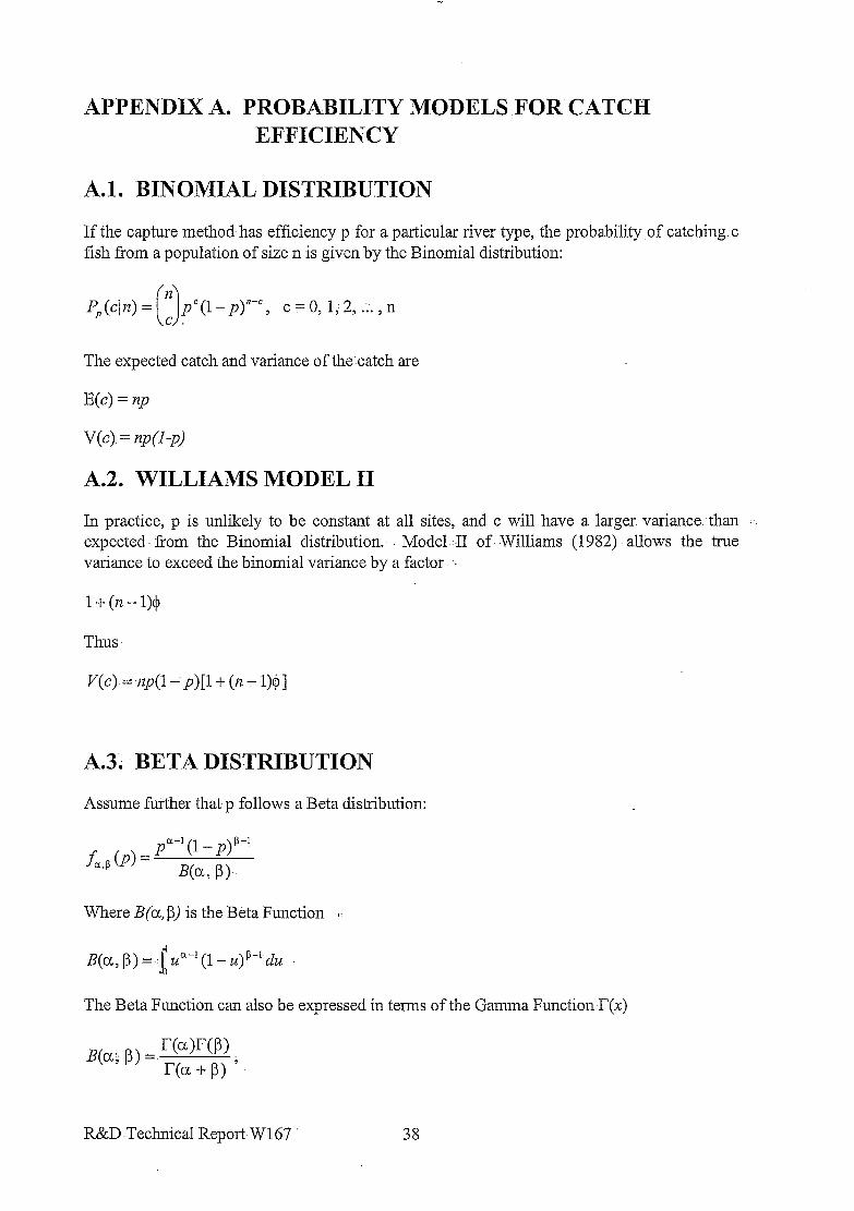
APPENDIX A. PROBABILITY MODELSFOR CATCH EFFICIENCY

A.1. BINOMIAL DISTRIBUTION

If the capture method has efficiency p for a particular river type, the probabilityof catching c fish from a population of size n is given by the Binomial distribution:

Pp (cl a) = 0. 1 pc (1 - p)‘-, c = 0, 1,2, .;. , n

The expected catch and variance of the-catch are

E(c) = np

VC> = nP(l-Pl

A.2. WILLIAMS MODEL II

In practice, p is unlikely to be constant at all sites, and c will have a larger variance than . . . expected- Tom the Binomial distribution. Model II of- Williams (1982) allows the true variance to exceed the binomial variance by a factor. ..

1 + (TZ - l)$

Thus

Y(c).=-7zp(l ‘p)[l f- (n - l)$]

A.3. BETA DISTRIBUTION

Assume further that p follows a Beta distribution:

f a.P

(p) = p”-‘(1 - PF’

B@, P>

Where B(a,Pj is the Beta Function- :.

The Beta Function can also be expressed in terms of the Gamma Function I+)

B@., p> = wow) ,

I-@ -l- p> ;


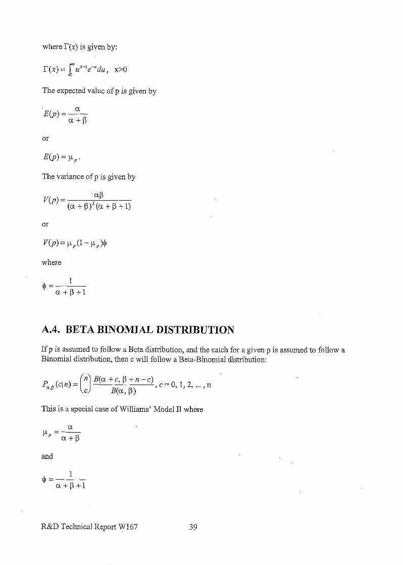
where I(X) is given by:

T(x) = p,Pe-Yzu, x>o

The expected value of p is given by

or

The variance of p is given by

Jw = ‘@ (a+P>2(Q+o+l>

or

where

A.4. BETA BINOlMIAL DISTRIBUTION

If p is assuined to follow a Beta distribution, and the catch for a given p is assumed to follow a Binomial distribution, then c will follow a Beta-Binomial distribution:

pa,p (~1 n) = ’ 0

B(a + ” ’ + n - ‘) , c = 0, 1, 2, . . . , n c W, P>

This is a special case of Williams’ Model II where

and


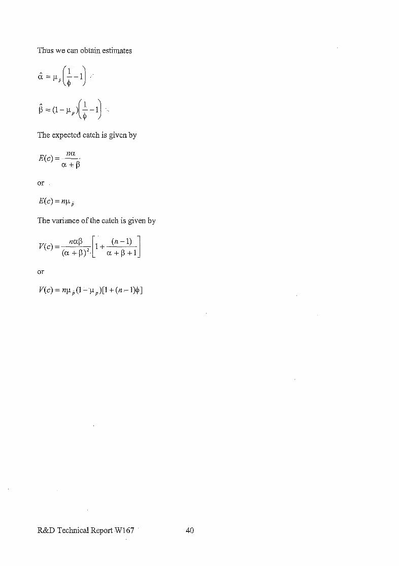
Thus we can obtain estimates

f&(1-pp) ( 1 i-1 . . . The expected catch is given by

or

The variance of the catch is given by

y(c) = (a 1+ (n-1) 1 a+p+1

or

Y(c) = np-lp (1 -‘Q[l -i (n .- l)$]


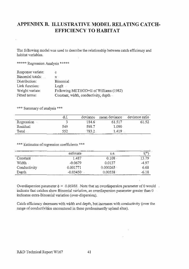
APPENDIX B. ILLUSTRATIVE MODEL RELATING CATCH- EFFICIENCY TO HABITAT

The following model.was used to describe the relationship between catch efficiency and habitat variables.

Response variate: C

Binomial totals: n . . . Distribution: Binomial Link function: Logit Weight variate: Following METHOD=II of Williams (1982) Fitted terms: Constant, width, conductivity; depth

d.f. deviance mean deviance deviance ratio Regression 3 184.6 61517 61.52 Residual 549 598.7 1.090 Total 552 783.2. 1.419

*** Estimates of regression coefficients **+

Constant Width, Conductivity Depth

estimate s.e. v+> 1.487 0.108 13.79

-0.0679 0.0137 -4.97 0.001771 0.000265 6.68 -0.03450. 0.00558 -6.18

Overdispersion parameter $I = 0.06988. Note that an overdispersion parameter of 0 would . indicate that catches show Binomial variation, an overdispersion parametergreater than 0 ‘. indicates extra-Binomial variation (over-dispersion).

Catch. efficiency decreases with width and depth,. but -increases with conductivity (over the range of conductivities encountered in these predominantly upland sites).


APPENDIX C. APPLICATION OF CATCH-EFFICIENCY MODEL TO A NEW SITE :

Consider a site 5m wide, with average depth 20cm, and conductivity 200: -From the catch- efficiency model in Appendix B we get

q = 1.487 -i- 5 x (-0.0679) +-20 x (-0.0345) + 200 x (0.001771-)-:

q = 0.8117

A logit link-function is used and so

q =-log, -!Ax- !. 1 l.- Pp therefore

pp-L 1 + e-n.

clp= 1 1. + e-o.8117 .

pp = 0.6925 :

This is the average capture efficiency for: trout par-r in sites .5m wide, with- average depth 20cm, and conductivity 200,uSlcm. Given the over-dispersion parameter, I$ = 0.06988, and assuming the over. dispersed binomial -follows a -Beta-Binomial model ‘(a special case .of Williams Model II; see Appendix A) we can obtain.estimates for a and p.

&-= 0.6925( o.o;g88 -1)

2 -= 9.22

b=(l-p,) i-1 ( 1

b = (1 - 0.6925) (0.061988 : ‘1

b = 4.09


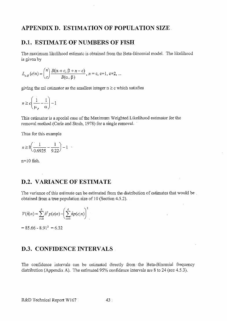
APPENDIX D. ESTIMATION OF POPULATION SIZE

D.1. ESTIMATE.%)F NUMBERSOF FISH

The maximum likelihood-estimate is obtained from the Beta-Binomial model; .The likelihood is given by

4&p (44 = 0 n ~@~~+cm-n-c> n=c c”l c+3

B(u,-p> ’ ’ ’ ’ d, . . . c

giving the ml estimator as the smallest integer n 2 c which satisfies

1 1 nrc --- -1 !’ 1 PP u

This estimator is a special case of the Maximum Weighted Likelihood estimator for the removal method (Carle and Strub, 1978) for a single removal.

Thus for this example

n=lO fish.

D.2: VARIANCE OF ESTIMATE

The variance of this estimate can be estimated from the distribution of estimates that would be obtained from a true population size of lO.(Section 4:5.2).

w4 4 = &?2p(c,n)- c=o

= 85.66.- 8.912 = 6.32

D.3. CONFIDENCE INTERVALS

The confidence intervals. can be estimated directly from. the Beta-Binomial frequency. distribution (Appendix A), The estimated 95% confidence intervals are 8 to 24 (see 4.5.3).

R&D Technical Report W167 43.

APPENDIX E. PROBABILITY MODELS FOR POPULATION SIZE.

E.1. POISSON DISTRIBUTION

If fish can be assumed. to be distributed randomly throughout a reach with average density 0, then the number of fish (n).within each unit of area will fol1ow.a Poisson distribution.-

p, (n) = q ) 72 = 0, 1,2, . . .

E(n) = 8

V(n) = 0

E;2. GAMMA DISTRIBUTION

Fish are rarely distributed in a random- fashion, but.instead show a clumped distribution. .This can be thought of as the density 8 itself ,. xu-ying randomly, and .following a Gamma distribution.

E(8) =-h

v(e) = h’/k

E.3. NEGATIVE BINOMIAL DISTRIBUTION

If the density of fish varies according to a Gamma distribution @2), and the number of fish. present in a site follows a Poisson distribution (E.l) for.: a given density, then the resulting distribution of population sizes (n) will follow a Negative Binomial distribution.

$..k (4 = ~&$$-J(&)“, n=OJA..

E(n).= h

V(n)= h( 1+1/k)

Note that when k = 1 we have the Geometric distribution,..and as k -+ co, we approach the Poisson distribution.

R&D Technical Report W 167 44 ‘I

APPENDIX F.’ ILLUSTRATIVE MODEL RELATING TROUT ABUNDANCE TO HABITAT

The expected population of fish will vary between river types. This was modelled using a Negative Binomial GLM, and variables for. access for sea trout(s), distance from river source (d) and gradient of river (g).

****I Regression .&alysis *****

Response variate: n Distribution: .. Negative binomial with parameter. k = 0.62 Link function:. Log. Offset variate: Log(area)- Fitted terms:. Constant+d.s+s+g+gg’+d

*** Summary of analysis ***

d.f. deviance : mean deviance

deviance ratio

Regression 5‘ 165;2. 33.032 32.63. Residual 596 603.4 1.012:: Total- 601 768.5 1.279

*** Estimates of regression coefficients***

Constant d.s S

g 2

:.

estimate s.e. t(596) -2.445 1 0.0874 -27.98 -0.0408 0.0170 -2.40

0.853 0.110 7.77 0.02443 0.00563 4.34

-0.0001930 -0.0327 0.0000741 0.0145 -2.60 -2.26

R&D Technical -Report W167 45

*** Accumulated analysis of deviance ***

Change

i-d.s +S f.3 +g’ +d Residual Total 601 768.547 1.279

d.f. deviance mean deviance deviance ratio

1 87.344 87.344 86.27 1 44.708 44.708 44.16 1 19.480 19.480 19.24

.L ’ 1 8.312 8.312 8.21 1 5.313 5.313 5.25

596 603.389 1.012

Trout parr densities are higher in streams where sea trout spawn (s=l) than in brown trout- only rivers (s=O). Densities show a quadratic relationship with river gradient (g, g’); in general, high gradients are preferred. Trout densities also reduce with increasing distance from source (d), and this relationship is different between sea trout and brown trout rivers (ds).


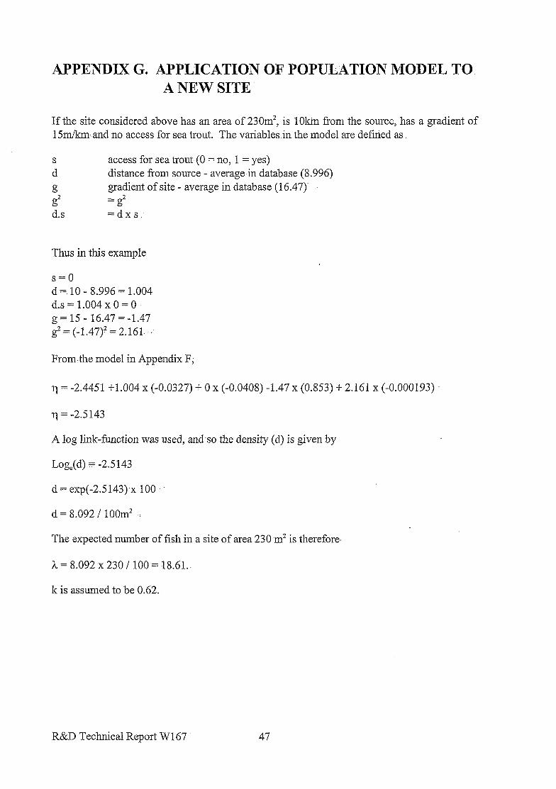
APPENDIX G. APPLICATION OF POPULATION MODEL TO.. A NEW SITE

If the site considered above has an area of 23Om’, is lOkin fi-om the source, has a gradient of 1 Sm/km:and no access for sea trout. The variables in the model are defined as.

S

d

g g2 d.s

access for sea trout (0 = no, 1 = yes) distance from source - average-in database (8.996) gradient of site - average in database (16.47) = g’

=dxs

Thus in this example

s=o d = 10 - 8.996 = 1.004 d.s = 1.004 x 0 = 0 g = 15 - 16.47 = -1.47 $=(-1.47)2=2.161--z’

From,the model in Appendix F,

q = -2.4451 +1.004 x (-0.0327) + 0 x (-0.0408) -1.47 x (0.853) + 2.161 x (-0.000193)

q = -2.5143

A log link-function was used, and so the density (d) is given by

Loge(d) 3 -2.5143

d = exp(-2.5 143) x 100

d = 8.092 / loom’. :

The expected number of fish in a site of area 230 m’ is therefore

h = 8.092 x 230 / 100 = 18.61.

k is assumed to be 0.62.


APPENDIX H. DERIVATION OF POSTERIOR DISTRIBUTION

From Bayes Theorem

P n$,;C,k w = L,p (cl 4ph.k (4

where

Pu;P,h,k (nl c) is the posterior distribution of n from-which the probability of class is calculated

La,p (cl 72) is the likelihood of the observed catch given a population size n, obtained from the-

capture-efficiency model.

Px,k (72) is the prior distribution of n, obtained from the abundance model

From Appendix A, the likelihood -is

&,p (Cl 4 = n B(a+c,p+n-c)~

0 , iz = c, c+l, c+2, . . .

c ST P> ”

From Appendix E, the prior distribution is

The un-normalised posterior distribution is therefore given-by

%,,,,,(4c) cc r(p It 72 - c)lT(k + n)Y

(n-c)!r(a+P+n)(h+k)” ’ I2 =~c~~c+1~c+2~ ***


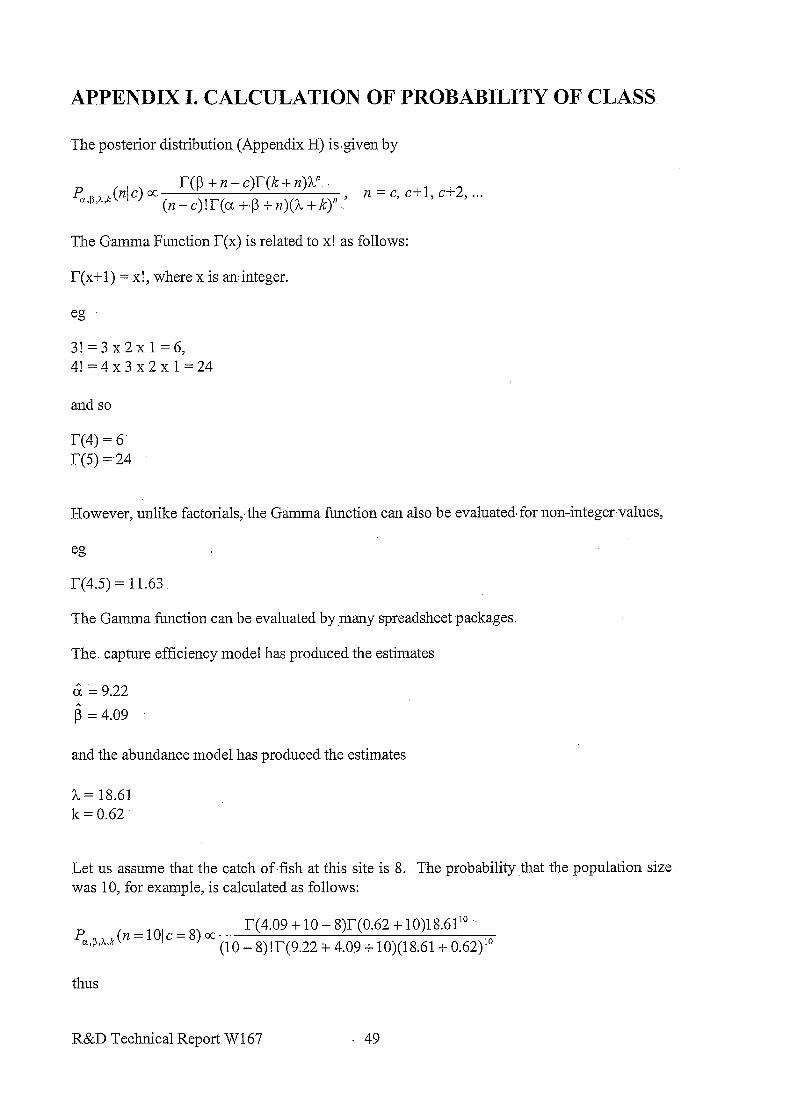
APPENDIX I. CALCULATION OF.PROBABILITY OF CLASS.

The posterior distribution (Appendix H),isgiven by

P u,P,l,k (4 4 cc I?@ +n-c)r(k+TZ)hn

(pq)!r(~+~p +Tg(h+/q” ,’ I2 = cJ c+ly ci2y-’

The Gamma FunctionT(x) is related to x! as follows:

lI(x+l) = x!, where x is an: integer.

eg

3!=3x2~1=6, 4! =‘4 x 3 x 2 x 1 = 24

and so

r(4)=6' r(5) = 24

However, unlike factorials, the Gamma function can also be evaluated-for non-integer values,

I-(4.5) =-11.63

The Gamma function can be evaluated by ,many spreadsheet packages.

The capture efficiency model has produced the estimates

& = 9.22

6 = 4.09

and the abundance model has produced the estimates

1” = 18.61 k = 0.62

Let us assume that the catch of-fish at this site is 8. The probability that the population size. was 10, for example,-is calculated as follows:

P a,P,h,,c (II= 101 c = 8) CC r(4.09 + 10 - 8)I(O.62 + 10)18.61io ”

(10 - S)!r(9.22 + 4.09 + 10)(18.61 f- 0.62)”

thus


P @,h,J (n=101c=8) = 0.0033

The posterior distribution is calculated from n = c, up to high values of n where the probabilities are very low:

P np,h,,c (n= 81c=8) 0~ 0.0019 P (Qq,; (n= 9jc=8) CJz 0.0031 Pa,p,h, (n=lOjc=8) cc 0.0033 P Q,hk (rz=l ljc=8) cc 0.0029 P cLp,)Lk (n=121c=8) cc 0.0024 P Q,hk (n=l3Jc=8) x 0.0019 PqQ+Q (n=14@8) cc 0.0014 P a,p,Q (n=lq=8) cfz 0.001 I

and so on.

The sum of these numbers (up to a high value of n) is 0.0209, and so to convert them to the posterior probabilities, it is necessary to divide by 0.0209, thus

P rQ,h,k (n= 8lc=8) = 0.0914 P9p,k,k (n= 9lc=8) = 0.1464 Pa,p,A,k (n=lOjc=8) = 0.1556 P gp,Q (n=l 1 Ic=S) - = 0.1393 PQ,AR (P.=12jc=8) = 0.1143 P ccp,hk (rz=131c=8) = 0.0893 P,J,~,~ (72=14lc=8) = 0.0678 P a,p,~,~ (72=15jc=8) = 0.0506

and so on.

These sum to 1 as required.

Applying the Agency classification of trout par-r densities (n/a per loom’).

Class A B C D E F

Density range n/a>21

21 kn/a> 12 122n/a> 5 52nIa> 2 22nfa> 0

n/a= 0


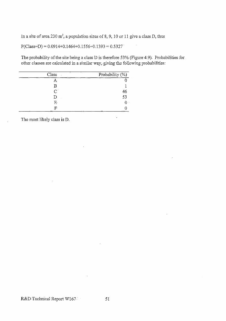
In a site of area 230 rn?; a population sizes of 8,9, 10 or 11 give a class D: thus

P(Class=D) = 0.0914+0;1464+0.1556+0.1393 = 0.5327

The probability of the site being a class D is therefore 53% (Figure.4.9); Probabilities for other classes are calculated in a similar way,.giving the following probabilities:

Class Probability (%) A 0 B 1 C 46 D 53 E 0 F 0

The most likely class is D.

R&D Technical Report W167’ 51

semi-quantitative methods for fisheries classification

Documents