sell-side analyst research and stock comovement rebello xu (2013).pdf · sell-side analyst research...

Sell-side Analyst Research and Stock Comovement∗

Volkan Muslu, Michael Rebello, and Yexiao Xu †

September 2013

Abstract

We document that analysts who cover a pair of stocks expect future earnings ofthe stocks to be more highly correlated than do analysts who cover only one of thestocks. Such coverage-based differences in analyst research impact stock prices in avariety of ways. Returns on a pair of stocks around a recommendation or a forecastare closer when the issuing analyst covers both stocks than only one stock in thepair. Stock returns around a recommendation revision covary with returns of otherstocks that the issuing analyst covers. In general, daily return correlations betweenstocks in a pair increase with the intensity of shared analyst coverage. Moreover,a stock’s daily returns are positively correlated with daily returns of other stocksthat share analyst coverage with the stock. Collectively, our evidence indicates thatshared analyst coverage is a channel for information spillovers that can raise returncomovement among stocks by an economically meaningful amount.

Key Words: Analyst coverage, Return correlation, Comovement, Spillover.

∗We are grateful to the editor, Philip Berger, an anonymous referee, Gus De Franco, Stan Markov, DavidReppenhagen, Daniel Taylor, Kelsey Wei, and seminar participants at Southern Methodist University, Universityof Houston, University of Texas at Dallas, 2011 FMA Asian conference, 2011 AAA annual conference, and 2012AAA FARS mid-year meeting for helpful comments.†University of Houston, University of Texas at Dallas, University of Texas at Dallas. Email: [email protected],

[email protected], and [email protected]

1. Introduction

Researchers are debating whether sell-side analysts primarily produce stock-specific or broad

(market- or industry-wide) information. Piotroski and Roulstone (2004) and Chan and Hameed

(2006) document that broad stock indices explain more of the returns of stocks with higher

levels of analyst coverage, suggesting that analysts convey primarily broad information. In

contrast, Liu (2011) finds that analyst recommendation revisions convey primarily stock-specific

information. Based on cross-sectional evidence, Crawford, Roulstone, and So (2012) show that

analysts convey primarily stock-specific (broad) information for stocks that are already covered

(not covered) by other analysts.

We join the debate by documenting that analysts also convey coverage-specific information,

i.e., information that emphasizes commonalities among stocks in their coverage. This informa-

tion, which has been overlooked by prior literature, lies within a wide spectrum whose opposite

extremes are marked by stock-specific and broad information.1 Consider analysts who con-

currently cover Oracle and SAP, stocks from the enterprise software segment of the computer

software industry. The analysts can produce information that is simultaneously useful in eval-

uating both stocks by, for example, focusing on software investments of client firms or new

software releases of competitors. This information is not specific to either Oracle or SAP, yet it

is more focused than information on the computer software industry or the market. Similarly,

analysts covering only large oil companies such as Exxon and Chevron can focus on shared issues

relating to vertical integration, issues which are largely irrelevant for small oil companies.

There are also ample opportunities for analysts to produce valuable coverage-specific infor-

mation when they cover stocks from multiple industries by, for example, emphasizing the linkages

between the stocks. Analysts covering both original design manufacturers (e.g., Dell) and origi-

1We have searched for explicit coverage-specific information in analyst reports for a small set of stocks in2010. The reports frequently contain references to other stocks analysts cover. Consistent with Franco, Hope, andLarocque (2012), most of these references are about competitors, suppliers, and customers. While consistent withthe use of coverage-specific information, this evidence is not conclusive since, in many cases, analysts who do notcover competitors, suppliers, or customers also mention these stocks. However, some references strongly suggestthe use of coverage-specific information. In these instances, analysts refer to other firms they cover that are notcompetitors, customers, or suppliers. Moreover, only these analysts appear to find these stocks relevant since otheranalysts do not mention these stocks. Examples of such references include one report that uses metrics for SAP andYahoo to justify the analyst’s valuation of Apple; an analysis of business ties between Discovery Communicationsand Mattel to justify the latter’s valuation; the use of metrics on H&R Block (tax services), Republic Services(waste management) and DigitalGlobe Inc (satellite imaging) to value Cintas Corp (industrial uniforms); metricson Arch Coal (coal mining) and Ashland Inc (chemicals) to evaluate Vulcan Materials (construction materials).

1

nal equipment manufacturers (e.g., Asustek) that supply components may focus on the supply

chain between these companies. Similarly, analysts covering stocks from different industries but

with common economic exposure, e.g., manufacturing bases in China, can highlight the effect of

this exposure.

We propose that analysts convey coverage-specific information because it can help achieve

an optimal balance between research costs and brokerage revenues tied to investor demand for

their research. Stock-specific research is costly because it requires an analyst to gather and

process information unique to each stock. To lower research cost per stock, an analyst can use

coverage-specific information rather than only stock-specific information. This substitution of

coverage-specific for stock-specific information will make the analyst’s research less informative

for the stock that is the subject of the research (stock X), but more informative for other

stocks the analyst covers. Consequently, investors interested in stock X will demand less of the

analyst’s research on stock X. However, this fall in demand will be mitigated because the price

of the research on stock X will likely fall to reflect its lower cost. Moreover, the coverage-specific

content of research on stock X will attract investors interested in other stocks the analyst covers,

broadening demand for the research.2 In equilibrium, the lower cost and price of coverage-specific

research, together with this broadening of demand, can make coverage-specific research more

profitable for the analyst. Consequently, an analyst will choose to convey information that is

common to stocks he covers rather than only stock-specific information when coverage-specific

research significantly lowers cost or increases aggregate investor demand. At the same time, the

analyst has weak incentives to only emphasize commonalities among stocks outside his coverage

since he is limited to spreading costs across the stocks he covers, and can expect to be rewarded

primarily for the value of his research on this limited set of stocks (Groysberg, Healy, and Maber,

2011; Krigman, Shaw, and Womack, 2001; Jackson, 2005; Ljungqvist et al., 2007).

Coverage-specific information will be used by many investors who seek cheap information that

is useful to evaluate other stocks (Veldkamp, 2006). Consequently, coverage-specific information

will raise average investor expectations about shared economic exposures among stocks that an

analyst covers. Investor responses to their changed expectations will, in turn, result in higher

2The argument about the broadening of the investor set in response to coverage-specific information is basedon Veldkamp’s (2006) argument about the complementarity in information demand across different assets.

2

return comovement than what covariance of stock fundamentals would predict, i.e., there will be

coverage-specific spillovers.3 We refer to these predictions collectively as the Coverage-Specific

Spillover Hypothesis.

We test the different predictions of this hypothesis using all stocks at the intersection of the

CRSP/Compustat and I/B/E/S databases between years 1997 and 2010. To control for stocks’

shared economic exposure, our tests either employ fixed stock pairs, focus on short-term returns

surrounding analyst activity, or employ a comprehensive set of controls that include correlations

between stocks’ past cash flows and earnings, and similarities in size, growth options, leverage,

performance, stock price levels, and shared industry, location, exchange, and S&P 500 index

membership. This research design is necessary to draw causal inferences about coverage-specific

spillovers since shared economic exposure can affect both analysts’ coverage choices and return

comovement (Kini et al., 2009; Hameed et al., 2012).

We first search for direct evidence of coverage-specific information in analyst research. For

each stock pair in a year, we identify analysts who cover both stocks in the pair (hereafter,

pair analysts) and those who cover only one stock in the pair (hereafter, individual analysts).

We then compare the correlation between the earnings forecasts for a stock pair issued by pair

analysts with the correlation between earnings forecasts issued by individual analysts for the

same stock pair. Any difference in the forecast correlations from pair and individual analysts for

the same pair of stocks must only be driven by differences in shared exposure estimates between

these two sets of analysts—and not by the stocks’ shared economic exposure. Since both forecast

correlations for a stock pair are based on the same shared economic exposure, this comparison

addresses concerns about reverse causality from shared economic exposure to analyst research

(Hameed et al., 2012). We find that the within-stock pair correlation between the earnings

forecasts from pair analysts are both meaningfully and statistically higher than those from

individual analysts. This difference indicates a stronger emphasis on shared economic exposure

by pair analysts, supporting the Coverage-Specific Spillover Hypothesis.

Our second set of tests examines short-term price responses to analyst activity (i.e., issuance

of a recommendation or a forecast) for evidence of coverage-specific information. We compare

3Investor expectations of shared economic exposure result in comovement between stock returns (Merton,1973).

3

how activity from pair and individual analysts for one stock in a pair (i.e., activity stock) affects

the return on the other stock (i.e., no-activity stock). Since the price responses to activity from

the two groups of analysts for the same stock pair will be based on the same fundamentals, this

comparison addresses concerns about reverse causality from shared exposure to analyst research

and investor responses (Hameed et al., 2012). We find that returns on the activity and no-activity

stocks are closer in response to activity by pair analysts than activity by individual analysts. The

economic and statistical significance of this difference suggests stronger information spillovers

from activity by pair analysts, supporting the Coverage-Specific Spillover Hypothesis.

By decomposing stock returns around recommendation revisions (Liu, 2011), we find that

coverage-specific information in analyst recommendations has a price impact comparable to that

of broad market- and industry-related information in the recommendations. We also find that

return correlations between the recommended stock and other stocks that share coverage by the

analyst making the recommendation are significantly higher than return correlations between

the recommended stock and other stocks that share coverage by inactive analysts. This finding

links coverage-specific spillovers directly to analyst activity.

In our final set of tests, we examine how shared analyst coverage affects correlation between

stocks’ daily returns during a year. The effect of shared coverage is apparent at the stock-pair

level: Stock pairs with higher shared coverage display greater return correlation even after we

introduce an exhaustive set of controls for shared economic exposure between the stocks in a

pair. In fact, daily return correlation of a stock pair is directly related to the estimates of shared

exposure conveyed in the earnings forecasts of pair analysts even after we control for estimates

of shared exposure conveyed in the earnings forecasts of individual analysts. Furthermore, a

portfolio of stocks with which a stock shares analyst coverage is a significant determinant of

the stock’s daily returns, and this relation is incremental to the effect of industry- and market-

returns. We find corroborating evidence in return synchronicity tests. Broad stock indices better

explain daily stock returns of individual stocks that share more analyst coverage with other

stocks. At the same time, the increased return synchronicity due to shared analyst coverage is

more concentrated on portfolios of stocks that share more analyst coverage. These results hold

even after we control for the effect of shared economic exposure as well as the level of analyst

coverage on return synchronicity (Piotroski and Roulstone, 2004; Chan and Hameed, 2006).

4

Consistent with the Coverage-Specific Spillover Hypothesis, all our findings indicate that

analyst research conveys coverage-specific information and this information spills over across

stocks that share analyst coverage. The coverage-specific spillovers are apparent even after we

control for shared economic exposure between the stocks. Our findings also support the existence

of broad and stock-specific information in analyst research. However, they are inconsistent with

analyst research exclusively conveying either of broad or stock-specific information, i.e., the

absence of coverage-specific information in analyst research.

Our paper contributes to the literature on the information content of analyst research. Secu-

rity analysts produce value-relevant information (Givoly and Lakonishok, 1979; Bhushan, 1989;

Lys and Sohn, 1990; Brennan, Jegadeesh, and Swaminathan, 1993; Francis and Soffer, 1997;

Frankel, Kothari, and Weber, 2006).4 Based on the ability of market- and industry-indices

to explain a stock’s returns (return synchronicity), Piotroski and Roulstone (2004) and Chan

and Hameed (2006) find that analysts primarily produce market- and industry-specific informa-

tion. In contrast, Liu (2011) shows that analysts primarily produce stock-specific information.

Hameed et al. (2012) reconcile these two seemingly contradictory findings by showing that

prices of stocks that are followed by more analysts are more accurate and that investors use

these prices to infer the values of less-researched stocks. Consequently, returns on stocks with

greater analyst following covary more strongly with market- and industry indices, giving the

appearance that analysts primarily produce broad information. We propose and find evidence

that analysts also produce information that focuses on commonalities among stocks they cover.

This coverage-specific information is distinct from stock-specific or broad market and industry

information discussed in the prior literature. Unlike spillovers of market- or industry-wide in-

formation, spillovers of coverage-specific information raises comovement only among stocks that

share analyst coverage. Moreover, coverage-specific information spillovers, as measured by in-

creases in return comovement, are of comparable magnitude to the effect of broad market or

industry information in analyst research.

Our paper also contributes to the literature on stock return comovement. Prior studies show

that return comovement between stocks in a pair is determined by similarities in size and book-

4Analysts also influence investments of portfolio managers (Walther, 1997; Falkenstein, 1996; Barber andOdean, 2008) and small investors (Malmendier and Shanthikumar, 2007; Mikhail, Walther, and Willis, 2007).

5

to-market ratio (Fama and French, 1993), cash flows (Chen, Chen, and Li, 2010), price level

(Green and Hwang, 2009), retail investor trading behavior (Kumar and Lee, 2006), industry

membership (Kallberg and Pasquariello, 2007), and stock index membership (Barberis, Shleifer,

and Wurgler, 2005).5 Nevertheless, Chen, Chen, and Li (2010) show that these determinants

cannot collectively explain a large portion of the variation in pair-wise daily return correlations.

We propose and show that, even after controlling for the determinants of return correlation

highlighted in this literature, the extent of shared analyst coverage can explain economically

meaningful variation in pair-wise return correlations.

The remainder of the paper is organized as follows. Section 2 develops the Coverage-Specific

Spillover Hypothesis. Section 3 describes the sample. Section 4 documents differences in the

information content of earnings forecasts issued by pair and individual analysts. Section 5 docu-

ments the short-term price effects of activity by pair and individual analysts. Section 6 describes

a battery of tests linking the level of shared analyst activity to daily return comovement. Section

7 provides concluding remarks. We provide detailed variable descriptions in the Appendix.

2. Coverage-specific spillover hypothesis

Veldkamp (2006) develops a rational expectations model to explain how investor demand

matches with analysts’ supply of information on different assets. The model demonstrates that,

when information production is costly, analysts can lower the cost of their research, and thus

its price, by producing information common to multiple assets. Investors demand such research

since they acquire it at a lower price and since it is informative for multiple assets. In equilibrium,

investors use research common to multiple assets more heavily than research specific to individual

assets. Consequently, returns on assets comove more strongly than can be justified based on the

covariance of their fundamentals alone.

We extend Veldkamp’s arguments to account for an important institutional feature: Each

analyst covers a limited number of stocks and is rewarded primarily for the value of his research

5Modern asset pricing theories (CAPM and Arbitrage Pricing Theory) build on the concept of covariance risk.Moreover, uncovering the determinants of return correlation among individual assets is of great interest to bothpractitioners and researchers working in the areas of portfolio management (Qian, Hua, and Sorensen, 2007), riskmanagement (Jorion, 2007), asset price dynamics (Rosenberg and Schuermann, 2006; Brooks, Henry, and Persand,2002), and trading strategies (Gatev, Goetzmann, and Rowenhorst, 2006; Papadakis and Wysocki, 2008).

6

on these stocks.6 From a cost perspective, an analyst can lower research costs per stock by

gathering and processing information relevant to multiple stocks in his coverage and spreading

the research costs accordingly. Since each analyst is limited to spreading the costs across the

stocks he covers, diversifying the scope of his research to stocks outside his coverage can yield few

additional savings. From a revenue perspective, the analyst can fully capture increased investor

demand by using coverage-specific information to widen the scope of his research only across

stocks he covers. Since the analyst cannot expect to be rewarded for increased investor activity

in stocks he does not cover, widening the scope of his research to stocks outside his coverage

will likely not be as profitable. Consequently, an analyst will choose to convey information that

is common to stocks he covers when there are significant cost reductions as well as increased

aggregate investor demand from this strategy.

If analysts produce, and investors use, coverage-specific research, then this research should

spill over to stocks that share coverage from the same analysts and promote comovement be-

tween the prices of these stocks. We refer to this hypothesis as the Coverage-Specific Spillover

Hypothesis and develop three related predictions that we elaborate below.

2.1. Coverage-specific research

According to the Coverage-Specific Spillover Hypothesis, analysts use information that is

common to the stocks they cover. Consequently, analysts who cover both stocks in a pair (i.e.,

pair analysts) are likely to develop their research using information that is common to the pair.

In contrast, analysts who cover one stock in a pair (i.e., individual analysts) will use information

that is less likely to be common to both stocks in the pair.7 Since earnings forecasts for a pair

of stocks will likely be more highly correlated when they are made using the same information

set, the earnings forecasts for a stock pair from pair analysts will be more highly correlated than

earnings forecasts from individual analysts.8

6By producing high-quality research on stocks they cover, analysts can attract new underwriting business(Krigman, Shaw, and Womack, 2001), generate brokerage income (Jackson, 2005), and earn “All-Star” recognition(Ljungqvist et al., 2007). Analysts earn higher compensation for each of these outcomes (Groysberg, Healy, andMaber, 2011).

7Although these analysts will also use information that is common to the stocks they cover, their research willinclude less information that is relevant for both stocks in the pair.

8Earnings forecasts issued by pair analysts may also differ from those issued by individual analysts for be-havioral reasons. Because coverage choices influence analysts’ information sets, they can influence the cues that

7

In contrast, correlations of earnings forecasts should not differ between pair and individual

analysts if their research lacks coverage-specific information, i.e., if the research exclusively con-

veys broad or stock-specific information. If both pair and individual analysts exclusively focus

on broad information, they will both base their research for each stock on market information

or information on the industry to which each stock belongs. Therefore, research from pair and

individual analysts will convey similar information about each stock in the pair. Similarly, if an-

alysts exclusively focus on stock-specific information, pair and individual analysts will produce

research on each stock that will be uninformative about the other stock in the pair. Conse-

quently, there should be no systematic difference between the correlations of earnings forecasts

issued by pair and individual analysts.

Research Prediction: Earnings forecasts for a pair of stocks will correlate more strongly if

analysts cover both stocks than if they cover only one stock in the pair.

2.2. Shared coverage and investor reactions

According to the Coverage-Specific Spillover Hypothesis, investors will react differently to

research from pair and individual analysts. Forecasts and recommendations from pair analysts

for one stock will be informative about both stocks in a pair, causing the price of the second

stock to comove with the price of the first stock. When an individual analyst issues a forecast

or recommendation for one stock in the pair, this activity will convey less information about the

second stock. Therefore, the price of the second stock will comove less with the price of the first

stock.

In contrast, investor reactions to research from pair and individual analysts should not differ

if analyst research exclusively conveys broad or stock-specific information. When analysts exclu-

sively focus on market or industry information, research on one stock from both types of analysts

will be similarly informative about the second stock, and therefore should elicit similar price re-

sponses for the second stock. If analysts exclusively focus on stock-specific information, research

from both types of analysts will be similarly uninformative about the second stock. Therefore,

analysts employ when estimating shared exposure between stocks. For example, analyst forecasts may be affectedby cue competition whereby analysts may underutilize salient cues because they are also presented with irrele-vant ones (Kruschke and Johansen, 1999; Hirshleifer, 2001). However, Chen and Jiang (2005) find that analysts’forecasts are driven by their incentives rather than behavioral biases.

8

the price of the second stock should not respond to research on the first stock regardless of

whether it is produced by pair or individual analysts.

Investor Reaction Prediction: Earnings forecasts or stock recommendations for one stock

in a pair will influence the price of the second stock more strongly if analysts cover both stocks

than if analysts cover one stock in the pair.

2.3. Shared coverage and return comovement

Analyst activity is not limited to publicly observable actions such as the forecast and rec-

ommendation announcements. We expect that analysts’ private communications with investors

will also influence investor perceptions of shared economic exposure. Therefore, according to

the Coverage-Specific Spillover Hypothesis, analyst research will spill over to stocks that share

coverage from the same analysts even when the analysts are not publicly active. Such informa-

tion spillovers are likely to increase with the number of analysts that cover the same stocks as

this will reinforce investor perceptions of shared economic exposure. Therefore, daily returns

on stocks with shared analyst coverage will covary more strongly as the level of shared coverage

rises.

In contrast, shared coverage should not affect daily return comovement when analysts ex-

clusively produce either broad or stock-specific information. If analysts exclusively produce

industry information, spillovers from their research should be systematically related to stocks’

industry membership, and if they produce market-wide information, the spillovers should be

similar across all stocks. In either case, the spillovers will not be systematically related to

the analysts’ coverage. If analysts exclusively produce stock-specific information, their research

should not convey information about other stocks.

Comovement Prediction: A stock’s return will comove more strongly with returns of other

stocks with which it shares more analyst coverage.

Prior research has demonstrated that analysts prefer to cover stocks that share economic

exposure with a larger set of stocks (Hameed et al., 2012), and follow portfolios that consist of

stocks with higher shared economic exposure (Kini et al., 2009). The reason for this preference

is clear: It is simpler to analyze a set of similar stocks than a set of diverse stocks. This

9

preference alone ensures that stocks that share analyst coverage will display more correlated

earnings forecasts as well as higher return correlation. The underlying cause of these relations

is shared economic exposure. In contrast, the premise of our predictions is that analyst research

generates information spillovers and thus return comovement. Therefore, to test the predictions

of the Coverage-Specific Spillover Hypothesis we have to control for the effect of shared economic

exposure. We take care to do so in all the tests we describe below.

3. Sample

We construct a comprehensive sample at the intersection of the CRSP/Compustat and

I/B/E/S databases. For each year between 1997 and 2010, we identify stocks that satisfy the

following criteria: (i) annual financials and daily returns should not have any missing observa-

tions; (ii) prices should be higher than $1 at the end of each month; (iii) at least one qualified

analyst should cover the stock. We define a qualified analyst as one who follows at most 40

stocks during the year (more than 99% of the I/B/E/S analysts), with the intent of removing

analyst teams and clerical errors.

Using the stocks that survive these filters, we generate all possible pairs of stocks for each

year. To find stock pairs with shared analyst coverage, we impose the following additional filter

on this universe of stock pairs: At least one qualified analyst should cover both stocks in each

pair by issuing a recommendation or earnings forecast for each stock in the pair. Collectively,

these criteria generate the largest possible sample of stock pairs with shared analyst coverage

that is relatively free of market microstructure effects. On average, this sample of stock pairs is

made up of 3, 518 stocks per year, representing more than 99% of the market capitalization of

all U.S. public stocks.

Insert Table 1 approximately here

Table 1 presents descriptive statistics for the sample. The sample includes 1,489,895 stock

pairs, which correspond to 106,421 stock pairs per year. On average, stocks in a pair are followed

by 23.4 analysts, 1.9 of whom are pair analysts. On average, analysts issue 19.7 recommendations

and 93.4 annual and quarterly earnings forecasts for each stock pair in a year. Pair analysts

account for 8.3% of the analysts covering a stock pair and 15.1% (15.6%) of the total number

10

of recommendations (forecasts) for a pair. We do not find a significant difference between the

per-stock recommendation or forecast frequencies of pair and individual analysts.

Panel A of Table 2 presents descriptive statistics for our sample stocks (49, 251 stock-years).

An average stock is covered by 9.2 analysts (Coverage) and shares analysts with an average of

60.5 other stocks. The sample stocks have total assets (Assets) of $6.1 billion, equity market

capitalization (Market Cap) of $4.1 billion, book value of equity (Equity) of $1.6 billion, and

annual trading volume (Volume) of 202.6 million shares. Additionally, 14% of the sample stocks

are included in the S&P500 index (S&P500 ). The sample average for liabilities deflated by

assets (Leverage) is 0.54, return-on-assets (ROA) is 0.00, earnings-per share (EPS ) is $0.83,

book-to-market ratio (BM ) is 0.69, stock price (Price) is $24.2, and age is 13.2 years (Age).

In untabulated results we find that firms in our sample are perceptibly larger than the other

CRSP/Compustat firms. The sample firms are also less levered, more profitable, older, and

enjoy higher valuations than other firms. These differences are not surprising, because analysts

are more likely to cover large and profitable firms (McNichols and O’Brien, 1997; O’Brien and

Bhushan, 1990; Rajan and Servaes, 1997).


Panel B of Table 2 presents descriptive statistics for the sample stock pairs. The pairwise

return correlation (Correlation) averages 0.269 and displays considerable variation: The 25th

percentile of Correlation is 0.121 while the 75th percentile is 0.393. The sample average of

Correlation is significantly higher than that for stock pairs that have no pair coverage (0.174).

Our measure of the prevalence of pair analysts, Pair Coverage, is the number of pair analysts

divided by the total number of analysts covering either stock in the pair. Pair Coverage falls

in the interval (0, 1], averages 0.102, and displays considerable variation: The 25th percentile

of Pair Coverage is 0.042 while the 75th percentile is 0.125. There are a small number of pairs

with Pair Coverage equal to one (1,786 pairs or 0.12% of the sample). More than 80% of these

pairs have only one analyst covering them.

We test the Research Prediction by comparing the within-stock pair correlations of monthly

consensus earnings forecasts issued by pair analysts and individual analysts. Using annual

earnings forecasts issued by pair analysts only, we construct a times series of monthly consensus

11

forecasts for each stock in the pair and compute the correlation between the two consensus

forecast series. We refer to this correlation as the Pair Forecast Correlation. We repeat this

process for annual earnings forecasts issued by individual analysts, and refer to the resulting

correlation as the Individual Forecast Correlation. We only use stock-pair-years with at least

three months with consensus earnings forecasts from individual and pair analysts for both stocks.

The average values of Pair Forecast Correlation and Individual Forecast Correlation are close at

0.099 and 0.100, respectively.9 Both sets of earnings forecast correlations are less than half the

average correlation in daily stock returns.

Our research design isolates the effect of coverage-specific spillovers on return comovement

between the stocks in a pair by controlling for the known determinants of return comovement

such as correlated trading and shared economic exposure. Panel B of Table 2 provides descriptive

statistics for these control variables. We control for the intensity of analyst coverage (Piotroski

and Roulstone, 2004; Chan and Hameed, 2006) using Coverage Intensity, which is the ratio of

the total number of analysts covering either stock in the pair to the average number of analysts

covering stocks from each of the pair’s two-digit SIC industries. Average Coverage Intensity is

1.29, indicating that the sample stocks enjoy higher than industry-average analyst coverage.

We also use the following indicator (dummy) variables as controls: Same Industry indicates

if pair stocks belong to the same two-digit SIC industry (Kallberg and Pasquariello, 2007);

Related Industry indicates if the pair stocks belong to industries that consume or supply 10%

of one another’s output as recorded in the Input-Output Benchmark Survey of the Bureau of

Economic Analysis (Menzly and Ozbas, 2010); Same Exchange indicates if pair stocks are listed

on the same exchange (Chen, Chen, and Li, 2010); Same State indicates if pair stocks are

headquartered in the same state (Chen, Chen, and Li, 2010); and S&P500 Members indicates if

pair stocks both belong in the S&P 500 index (Barberis, Shleifer, and Wurgler, 2005; Greenwood,

2008).

Same Industry and Related Industry average 43.4% and 18.1%, respectively. The remaining

stock pairs, which belong to different and unrelated industries, make up a significant portion of

the sample (38.5%), consistent with Clement (1999) and Kini et al. (2009). Same Exchange has

9Note that these observations include pairs where the two stocks’ fiscal year ends are far apart, making directcomparisons between these two correlations noisy. We compare Pair Forecast Correlation with Individual ForecastCorrelation in Section 4.

12

an average value of 59.7%, suggesting a strong likelihood that pair stocks are listed on the same

exchange. Same State has an average value of 13.9%, consistent with the clustering of firms

in a few states. S&P500 Members averages 7.6%. This is higher than the case if stock pairs

were formed randomly (1.7% = 14%× 14%), likely because more analysts cover S&P 500 stocks

(Veldkamp, 2006; Jegadeesh et al., 2004).

The second set of control variables captures the effect of similarities in stock characteristics

on return correlation (Chen, Chen, and Li, 2010). This set is made up of the following indicator

variables that equal one (zero) if characteristics of both stocks in a pair fall (do not fall) in

the same quartile of the sample stocks during a year: Similar Asset, Similar BM, Similar Age,

Similar Leverage, Similar ROA, Similar EPS, and Similar Price capture similarities in Assets,

BM, Age, Leverage, ROA, EPS, and Price, respectively. Average values of these indicators

range between 0.32 and 0.40, suggesting that a larger percentage of the pairs are formed of

stocks with similar characteristics than would be the case if pairs were formed randomly, 0.25

(= 4 × 0.25 × 0.25). The likely reason for this difference is the propensity of analysts to focus

their coverage on firms with similar characteristics, especially large and visible firms (Kini et al.,

2009; Hameed et al., 2012).

The third set of controls is designed to capture the effect of shared economic exposure. ROA

Correlation is the correlation in quarterly ROA between years t− 4 and t (Chen, Chen, and Li,

2010; Allayannis and Simko, 2009). To mitigate outliers, values of ROA greater than 10 or less

than -10 are set to 10 and -10, respectively. ∆ROA Correlation is the correlation in quarterly

changes in ROA between years t− 4 and t. EPS Correlation is the correlation in quarterly EPS

between years t− 4 and t, and ∆EPS Correlation is the correlation in quarterly changes in EPS

between years t − 4 and t. The average ROA Correlation (EPS Correlation) is 0.124 (0.115)

indicating that pair stocks share a limited amount of performance-related exposure. The average

values of ∆ROA Correlation and ∆EPS Correlation are perceptibly lower at 0.057 (0.063).

Untabulated correlation statistics show that Correlation is positively associated with Pair

Coverage (0.11) as well as all the measures of shared exposure and correlated trading. Pair

Coverage is negatively correlated with Coverage Intensity (-0.33) and Related Industry (-0.07),

but positively correlated with all other measures of shared exposure and correlated trading. Pair

Coverage is most highly correlated with Same Industry (0.20).

13

Finally, to ensure that our tests isolate and compare the information conveyed in research

of pair and individual analysts rather than the characteristics of these two groups of analysts,

we control for a set of pair-wise differences in analyst characteristics. Table 2, Panel C presents

these analyst characteristics. First, we control for the difference in the logarithms of average

experience of pair and individual analysts covering the pair (Diff Experience), because analyst

experience can affect both the quality of an analyst’s research as well as investor responses

to the research (Mikhail, Walther, and Willis, 2003).10 On average, pair analysts have been

on the I/B/E/S database longer (Experience, 7.2 versus 6.5 years). Second, we control for the

difference in the average size of brokers (i.e., logarithm of the number of employed analysts) that

employ pair and individual analysts covering the pair (Diff Broker Size), because broker size can

affect the resources available to analysts and the analysts’ ability to disseminate their research

(Clement, 1999). Pair analysts work for brokers that employ fewer analysts (Broker Size, 52.5

versus 56.5 analysts). Third, we control for the difference in the logarithms of average number of

stocks covered by pair and individual analysts (Diff Companies), because the number of stocks

covered is inversely related with research resources (Clement, 1999).11 Pair analysts cover more

stocks (Companies, 20.8 versus 16.1 stocks). Finally, we control for the difference in average

forecast errors between these two analyst groups (Diff Forecast Error), because past forecast

accuracy is related with investor perceptions about the research quality (Mikhail, Walther, and

Willis, 1999). We measure each analyst’s (in)accuracy using Forecast Error, the median absolute

forecast errors across all stocks the analyst covers during a year. Absolute forecast error is defined

as the absolute difference between an annual forecast and actual earnings per share deflated by

the share price at the beginning of the fiscal year. Average Forecast Error for pair analysts

and individual analysts are 0.58% and 0.64%, respectively, suggesting that pair analysts forecast

more accurately, consistent with their longer experience.

10Whenever we use logarithms of variables, we take the logarithm of one plus the variable.11We do not control for differences in pair and individual analyst activity per covered stock since there is no

meaningful difference between the per stock forecast or recommendation frequency of pair and individual analysts.

14

4. Forecast correlations

The Coverage-Specific Spillover Hypothesis predicts that analysts will highlight economic

exposure shared by stocks in their coverage. Consequently, earnings forecasts from analysts

who cover both stocks in a pair will correlate more strongly than earnings forecasts from an-

alysts who cover only one stock (Research Prediction). We test the Research Prediction by

examining the difference between the annual correlations of monthly consensus forecasts of pair

analysts and individual analysts. Since the same shared economic exposure underpins both sets

of forecasts, differences between the two sets of forecasts for the same stock pair can only result

from differences in the economic exposure highlighted by the two sets of analysts. Therefore, a

within-stock pair comparison of the consensus forecasts issued by pair and individual analysts

effectively controls for reverse causality from shared economic exposure to earnings forecasts.

Figure 1 plots (across deciles of Pair Coverage) average Pair Forecast Correlation and In-

dividual Forecast Correlation, which measure the correlation between the pair and individual

analysts’ consensus earnings forecasts for the two stocks, respectively. The figure also plots the

average pair-wise difference of the two consensus correlation measures, Diff Forecast Correlation.

In order to obtain a meaningful forecast correlation difference, we require that both forecast cor-

relation measures are constructed using at least eight overlapping months. This filter reduces

the number of observations from 688,755 to 568,307. Untabulated tests show that this filter

has no meaningful effect on our results. Both average Pair Forecast Correlation and Individual

Forecast Correlation increase with Pair Coverage.12 This is consistent with the evidence in Kini

et al. (2009) that analysts follow portfolios of stocks with high levels of shared exposure.

As is clear from the figure, Pair Forecast Correlation is either similar to or larger than Indi-

vidual Forecast Correlation. The difference between the two correlation measures monotonically

increases with Pair Coverage until its highest decile. This difference is statistically significant

when Pair Coverage is greater than 20%. The average difference between the two correlation

measures across deciles where Pair Coverage is greater than 20% is 3.6%, and is economically

12Only in the last decile of Pair Coverage do we observe a decline in the forecast correlations. This is likely aresult of the fact that stock pairs in this range have a small number of individual analysts (1.5) and the numberof pair analysts drops dramatically from 17.5 for the previous Pair Coverage decile to 8.1. Since the time seriesof monthly consensus earnings forecasts are likely to be updated less frequently when there are fewer analysts,this drop in the number of pair and individual analysts is likely to mechanically lower the precision of the twoforecast correlation estimates and bias them towards zero.

15

significant given that Pair Forecast Correlation and Individual Forecast Correlation average 23%

over this range of Pair Coverage. The relatively small difference for the two lowest Pair Cover-

age deciles may arise because the consensus forecast for pair analysts changes infrequently when

there are only a few pair analysts (1.8 on average), lowering the precision of the correlation

estimates and biasing them downwards. Overall, this evidence is consistent with the Research

Prediction that research from pair analysts will signal higher shared economic exposure than

research from individual analysts.

Insert Figure 1 approximately here

In order to understand the cross-sectional variation in the difference between pair and indi-

vidual forecast correlation, we estimate the following regression model:

Diff Forecast Correlationij,t = α+ β Pair Coverageij,t + γ Xij,t + εij,t, (1)

where X represents a vector of pair-wise controls for shared economic exposure, correlated

trading, and analyst characteristics. Table 3 presents OLS estimates of Eq. (1) with t-statistics

based on robust standard errors clustered by stock pair and year (Petersen, 2009). Model 1

includes controls for industry, geographical and exchange linkages, and shared membership in the

S&P 500 index. Model 2 adds controls for similarities in operating and financial characteristics of

the stock pairs. Model 3 adds controls for shared economic exposure as reflected in correlations

between measures of operating performance. Finally, Model 4 includes controls for differences

in the characteristics of pair and individual analysts.


According to the Research Prediction, the earnings forecasts from pair analysts will display

a higher level of correlation. As Pair Coverage increases, the frequency of changes in and thus

the precision of the consensus earnings estimates from pair analysts should rise. These changes

should mitigate the downward bias in Pair Forecast Correlation when Pair Coverage is low,

which is apparent from Figure 1. Therefore, we expect a positive β in Eq. (1).

Consistent with Figure 1, the coefficient estimates on Pair Coverage are uniformly positive

and significant at the 1% level. Moreover, the coefficient estimates on Pair Coverage show

16

only small changes ranging from 8.69 to 9.07 across the models. Economically, when Pair

Coverage increases from the first quartile (0.042) to the third quartile (0.125) of the sample, the

difference in consensus forecast correlations of pair and individual analysts widens by 0.8% (=

9.07% × (0.125 − 0.042)). This is a significant impact, given that it equals 8% of the average

forecast correlation for pair and individual analysts, which is around 0.100.

Few controls have statistically significant coefficient estimates, indicating that Diff Fore-

cast Correlation displays limited cross-sectional variation. The coefficient estimates on Similar

ROA, ROA Correlation, and EPS Correlation are negative and significant, suggesting that Diff

Forecast Correlation is smaller for pairs with greater shared economic exposure. This finding in-

directly supports the Coverage-Specific Spillover Hypothesis, since it suggests that pair analysts’

estimates are highly correlated regardless of the shared exposure of the stocks in a pair while

those of individual analysts are sensitive to the shared exposure. The coefficient estimate on

Diff Forecast Error is positive and significant, suggesting that the higher correlation in forecasts

of pair analysts may be associated with higher forecast errors. This is to be expected if pair

analysts rely more on coverage-specific information than stock-specific information.

These results are robust to the following changes in test specifications: using a count of

pair analysts instead of Pair Coverage; using a count of individual analysts instead of Coverage

Intensity ; using alternative industry definitions, e.g., two-digit I/B/E/S S/I/G industries or

two-digit GICS codes; focusing only on stock pairs from the same industry or different indus-

tries; replacing the dummy variables with continuous measures of similarities/difference in pair

characteristics; switching from clustering by year and stock pair to using year and stock-pair

fixed effects. We have ensured that all the subsequent results are also robust to these changes

in test specifications.

5. Investor reaction to analyst activity

According to the Investor Reaction Prediction, pair analyst research on one stock in a pair

will convey more information about the second stock than research from an individual analyst.

Consequently, short-term price reactions of the stock for which a recommendation or forecast is

issued (i.e., the activity stock) and the other stock in the pair (i.e., the no-activity stock) should

17

be closer, when a pair analyst issues the recommendation or forecast than when an individual

analyst does so. In contrast, if analysts rely exclusively on broad information or stock-specific

information, the gap in price reactions between the activity and no-activity stocks should not

differ between pair and individual analysts. This is because research on the activity stock from

both groups of analysts will be equally informative about the no-activity stock.

5.1. Difference-in-difference tests

In order to test the Investor Reaction Prediction, we benchmark the price responses to

research from pair analysts against the price responses to research from individual analysts

covering the same stock pair. Since the same shared economic exposure underpins both sets of

price responses, we effectively control for reverse causality from shared economic exposure to

price responses. To implement the difference-in-difference test, we first identify days on which

analysts issue recommendations or forecasts for only one stock in a pair (activity stock) for

each stock pair-year. We refer to these days as activity days (N = 31, 683, 028). We then drop

observations where the absolute value of one-day NYSE size decile-adjusted returns on either

the activity or no-activity stock are greater than 95th percentile of the population of activity-day

returns (that is, 6.8%).13 The resulting sample includes 30, 098, 877 activity days from 1, 292, 253

pair-years.

We measure the short-term price response to analyst activity for each activity day in two

ways. First, we compute the absolute value of NYSE size decile-adjusted returns of the activity

stock and the no-activity stock (Absolute Return). Second, we filter out the variation in innate

daily return volatilities of individual stocks by computing an activity-day analyst informativeness

(AI ) measure as follows (Frankel, Kothari, and Weber, 2006): For stock i in the pair ij, we

compute average absolute size-adjusted returns on all no-activity trading days during the year,

RNi , where

RNi =

∑TijRi,t

#Tij, (2)

Ri,t is the absolute size-adjusted return of stock i on day t, Tij is the set of no-activity days for

13We use this filter in order to remove the effect of significant events other than analyst activity such as macroe-conomic news, company news, or company disclosures. Since we are using absolute returns, we are effectivelydropping observations from the two tails of the actual distribution of daily returns.

18

the pair ij, and #Tij is the number of no-activity days. Then, on each activity day for the pair

ij, we compute stock i’s AI as follows:

AIiij =Absolute Returni

RNi

. (3)

If analyst activity is (is not) informative, then AI should exceed (equal) one on average.

Panel A of Table 4 presents mean and median values of Absolute Return and AI for activity

and no-activity stocks. The last two columns present differences between the two price response

measures for activity and no-activity stocks. Similarly, the last two rows present differences

between Absolute Return and AI for pair and individual analysts. The intersection of the last

two rows and last two columns reports the difference-in-difference tests. Specifically, each cell

in the intersection compares the difference in price reactions for the activity and no-activity

stocks in response to pair analyst activity with the difference in price reactions in response

to individual analyst activity. This differential price reaction between activity and no-activity

stocks measures the spillover from analyst activity; a smaller difference in Absolute Return or

AI indicates a smaller difference in the price responses and, thus, a larger spillover.


The results in Panel A provide strong support for the Investor Reaction Prediction. For days

during which pair analysts are active, the average Absolute Return (AI) is 1.73% (1.109) for

the activity stock and 1.60% (0.972) for the no-activity stock. For days during which individual

analysts are active, the average Absolute Return (AI) is 1.86% (1.175) for the activity stock

and 1.56% (0.966) for the no-activity stock. As expected, for both pair and individual analysts,

Absolute Return and AI are uniformly higher for the activity stock than the no-activity stock.14

Moreover, Absolute Return and AI for pair analysts are lower for the activity stock and higher

for the no-activity stock. This pattern is consistent with two corollaries of the Coverage-Specific

Spillover Hypothesis. First, pair analysts provide less stock-specific information. Second, pair

analysts provide more coverage-specific information.

14The AI for the no-activity stock is lower than one in response to activity from both pair and individualanalysts. One reason for this could be that investors shift their attention to the activity stock for which theanalyst activity is likely to be more informative and thus dampen price movements in the no-activity stock.

19

The difference-in-difference tests are consistent with the existence of stronger spillovers from

pair analyst activity. For pair analysts, the average pair-wise Absolute Return (AI) difference

between the activity and no-activity stock is 0.14% (0.138). In comparison, for individual ana-

lysts, the average pair-wise Absolute Return (AI) difference between the activity and no-activity

stock is significantly larger at 0.31% (0.208). Moreover, the difference-in-difference measures are

both statistically and economically significant: The average and median difference-in-difference

in stock price reactions between pair and individual analysts range between 4% to 10% of the

price responses of the activity stock. We conclude that, holding everything else constant, the

reaction of no-activity stocks is significantly stronger to research from pair analysts than re-

search from individual analysts. This supports the Investor Reaction Prediction and directly

links coverage-specific spillovers to analyst activity.15

In order to examine cross-sectional variation in price responses to research from pair and

individual analysts, we also estimate the following model:

Diff Absolute Returnij,t = α+ β Pair Coverageij,t + γ Xij,t + εij,t,

Diff AIij,t = α+ β Pair Coverageij,t + γ Xij,t + εij,t, (4)

where Diff Absolute Return (Diff AI ) is the pair-wise difference-in-difference between the aver-

age Absolute Return (AI) of the activity and no-activity stocks across the pair and individual

analysts. X represents the vector of pair-wise controls from Table 3.

Panel B of Table 4 presents OLS estimates of Eq. (4) with t-statistics based on robust

standard errors clustered by stock pair and year. When the dependent variable is Diff Absolute

Return, the coefficient estimates on Pair Coverage range from 0.181 to 0.286, and are significant

at the 1% level. When Pair Coverage increases from the first quartile (0.042) to the third quartile

(0.125) of the sample, Diff Absolute Return widens by 0.02% (= 0.286×(0.125−0.042)) in Model

4. This is an economically significant impact, given that average Diff Absolute Return is 0.17%.

When the dependent variable is Diff AI, the coefficient estimates on Pair Coverage range from

15In untabulated tests, we find that the results we report are robust to the following changes: using the ratiosrather than differences of the two activity day price reactions; using returns within a three day announcementwindow to capture price responses to analyst activity; and focusing on price responses to earnings forecasts orrecommendations alone.

20

0.093 to 0.177, and are significant at the 1% level. When Pair Coverage increases from the first

quartile to the third quartile of the sample, Diff AI widens by 0.015 (= 0.177× (0.125− 0.042))

in the Model 4. This is an economically significant impact, given that average Diff AI is 0.071.

The positive relation between spillovers and Pair Coverage may arise because increased exposure

to research from pair analysts conditions investors to believe that a stock pair has greater shared

exposure. This argument is supported by untabulated results which indicate that the difference

between the price responses of the activity and no-activity stock to individual analyst activity

are more sensitive to Pair Coverage.

Several control variables have statistically significant estimates, indicating that the difference

in spillovers between pair and individual analysts displays some cross-sectional variation. Same

Industry, Related Industry, Diff Experience, and Diff Broker Size are associated with an increase

in the relative strength of spillovers from pair analyst research, while S&P500 Members, Similar

Asset, Similar Age, Similar ROA, Similar EPS, Similar Price, and Diff Companies are associated

with a reduction in the relative strength of spillovers from pair analyst research.

5.2. Decomposing price effects of analyst activity

If a recommendation revision from an analyst for one stock is informative about other stocks

the analyst covers, the prices of the other stocks should also respond to the recommendation

revision. Therefore, returns around an analyst’s recommendation revision for a stock should be

correlated with returns on other stocks that the analyst covers. To test this prediction, we build

on the methodology in Liu (2011) to decompose stock returns around analyst recommendation

revisions into market, industry, shared coverage, and the residual stock-specific components.

Specifically, we estimate the following regression for each stock (i)-analyst (a) combination using

daily (t) returns during the calendar year:

Returnia,t = αia + βAia × Analyst Portfolioia,t

+ βMia × Market Portfoliot + βIia × Industry Portfolioi,t + εia,t, (5)

where Market Portfolio is the daily CRSP value-weighted market return, Industry Portfolio is the

daily value-weighted two-digit SIC industry return orthogonalized relative to Market Portfolio,

21

and Analyst Portfolio is the daily equal-weighted return on a portfolio of all the other stocks

covered by analyst a orthogonalized relative to Market Portfolio and Industry Portfolio.16

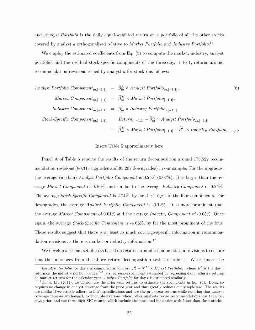
We employ the estimated coefficients from Eq. (5) to compute the market, industry, analyst

portfolio, and the residual stock-specific components of the three-day, -1 to 1, returns around

recommendation revisions issued by analyst a for stock i as follows:

Analyst Portfolio Component ia,[−1,1] = β̂Aia × Analyst Portfolioia,[−1,1], (6)

Market Component ia,[−1,1] = β̂Mia × Market Portfolio[−1,1],

Industry Component ia,[−1,1] = β̂Iia × Industry Portfolioi,[−1,1],

Stock-Specific Component ia,[−1,1] = Returni,[−1,1] − β̂Aia × Analyst Portfolioia,[−1,1]

− β̂Mia × Market Portfolio[−1,1] − β̂Iia × Industry Portfolioi,[−1,1].


Panel A of Table 5 reports the results of the return decomposition around 175,522 recom-

mendation revisions (80,315 upgrades and 95,207 downgrades) in our sample. For the upgrades,

the average (median) Analyst Portfolio Component is 0.25% (0.07%). It is larger than the av-

erage Market Component of 0.16%, and similar to the average Industry Component of 0.25%.

The average Stock-Specific Component is 2.74%, by far the largest of the four components. For

downgrades, the average Analyst Portfolio Component is -0.12%. It is more prominent than

the average Market Component of 0.01% and the average Industry Component of -0.05%. Once

again, the average Stock-Specific Component is -4.66%, by far the most prominent of the four.

These results suggest that there is at least as much coverage-specific information in recommen-

dation revisions as there is market or industry information.17

We develop a second set of tests based on returns around recommendation revisions to ensure

that the inferences from the above return decomposition tests are robust. We estimate the

16Industry Portfolio for day t is computed as follows: RIt − β̂IM × Market Portfoliot, where RI

t is the day t

return on the industry portfolio and β̂IM is a regression coefficient estimated by regressing daily industry returnson market returns for the calendar year. Analyst Portfolio for day t is estimated similarly.

17Unlike Liu (2011), we do not use the prior year returns to estimate the coefficients in Eq. (5). Doing sorequires no change in analyst coverage from the prior year and thus greatly reduces our sample size. The resultsare similar if we strictly adhere to Liu’s specifications and use the prior year returns while ensuring that analystcoverage remains unchanged, exclude observations where other analysts revise recommendations less than tendays prior, and use three-digit SIC returns which exclude the stock and industries with fewer than three stocks.

22

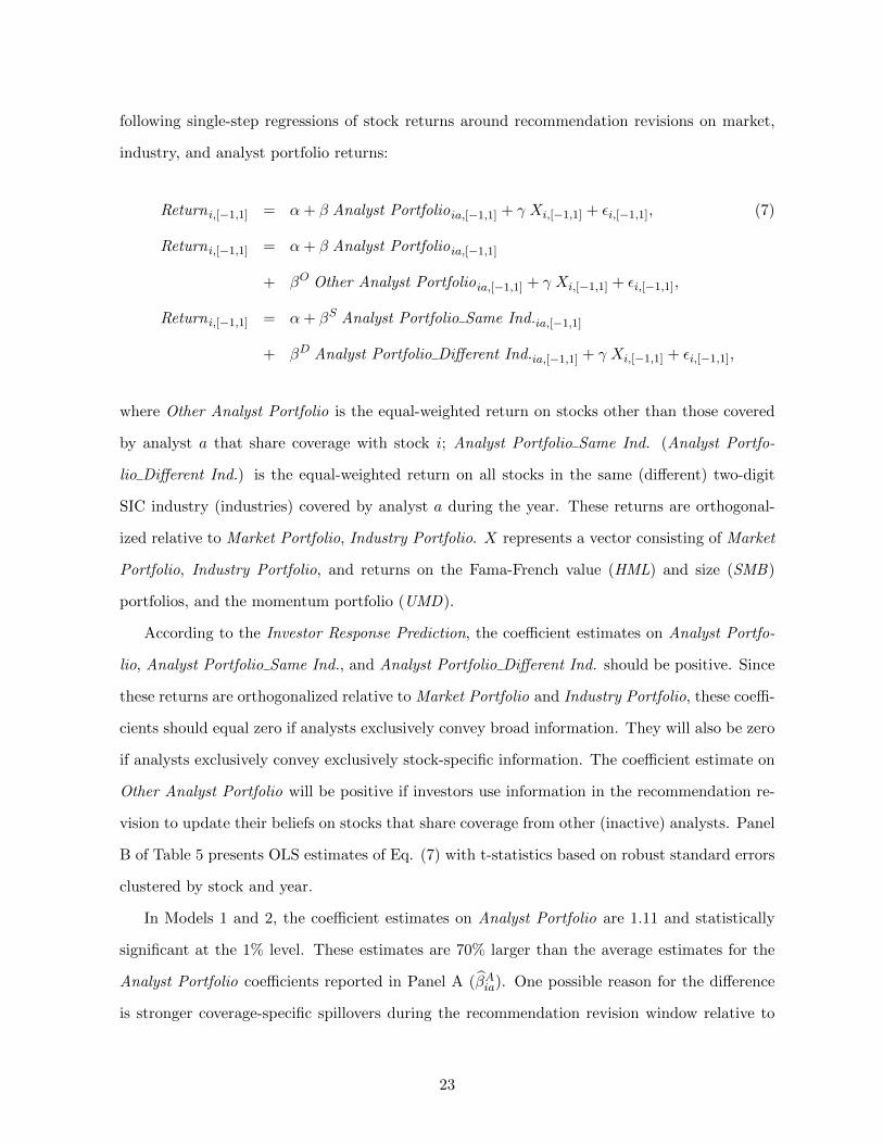
following single-step regressions of stock returns around recommendation revisions on market,

industry, and analyst portfolio returns:

Returni,[−1,1] = α+ β Analyst Portfolioia,[−1,1] + γ Xi,[−1,1] + εi,[−1,1], (7)

Returni,[−1,1] = α+ β Analyst Portfolioia,[−1,1]

+ βO Other Analyst Portfolioia,[−1,1] + γ Xi,[−1,1] + εi,[−1,1],

Returni,[−1,1] = α+ βS Analyst Portfolio Same Ind.ia,[−1,1]

+ βD Analyst Portfolio Different Ind.ia,[−1,1] + γ Xi,[−1,1] + εi,[−1,1],

where Other Analyst Portfolio is the equal-weighted return on stocks other than those covered

by analyst a that share coverage with stock i; Analyst Portfolio Same Ind. (Analyst Portfo-

lio Different Ind.) is the equal-weighted return on all stocks in the same (different) two-digit

SIC industry (industries) covered by analyst a during the year. These returns are orthogonal-

ized relative to Market Portfolio, Industry Portfolio. X represents a vector consisting of Market

Portfolio, Industry Portfolio, and returns on the Fama-French value (HML) and size (SMB)

portfolios, and the momentum portfolio (UMD).

According to the Investor Response Prediction, the coefficient estimates on Analyst Portfo-

lio, Analyst Portfolio Same Ind., and Analyst Portfolio Different Ind. should be positive. Since

these returns are orthogonalized relative to Market Portfolio and Industry Portfolio, these coeffi-

cients should equal zero if analysts exclusively convey broad information. They will also be zero

if analysts exclusively convey exclusively stock-specific information. The coefficient estimate on

Other Analyst Portfolio will be positive if investors use information in the recommendation re-

vision to update their beliefs on stocks that share coverage from other (inactive) analysts. Panel

B of Table 5 presents OLS estimates of Eq. (7) with t-statistics based on robust standard errors

clustered by stock and year.

In Models 1 and 2, the coefficient estimates on Analyst Portfolio are 1.11 and statistically

significant at the 1% level. These estimates are 70% larger than the average estimates for the

Analyst Portfolio coefficients reported in Panel A (β̂Aia). One possible reason for the difference

is stronger coverage-specific spillovers during the recommendation revision window relative to

23

days during which analysts are not active. Moreover, the announcement returns are at least as

strongly related to Analyst Portfolio as they are to market and industry returns. Specifically,

when Analyst Portfolio increases from its first quartile (−0.9%) to its third quartile (0.8%),

the announcement return rises by 1.9%(= 1.109 × (0.8% − (−0.9%))) in Model 2, which equals

22% of the interquartile variation in the announcement return. In comparison, changing Market

Portfolio from its first to third quartile raises the announcement return by 2.9%(= 1.175 ×

(1.3%− (−1.1%))) or 34% of the interquartile variation in the announcement return. Changing

Industry Portfolio from its first to third quartile raises the announcement return by 2.0%(=

1.213×(0.9%−(−0.7%))), which is nearly 23% of the interquartile variation in the announcement

return. Like Panel A, these results suggest that the coverage-specific information in analysts’

recommendation revisions is comparable to the amount of market or industry information the

recommendation revisions convey.18

In Model 3, we introduce Other Analyst Portfolio as an additional explanatory variable. This

captures the returns on stocks that share coverage from other analysts and thus are likely to have

similar levels of shared economic exposure but are not the subject of coverage-specific information

produced by the recommending analyst. Consequently, by comparing the coefficient estimates

on Other Analyst Portfolio and Analyst Portfolio, we can assess the extent of coverage-specific

information in the recommendation revisions. The coefficient estimate on Analyst Portfolio drops

to 0.742 but remains statistically significant at the 1% level. The coefficient on Other Analyst

Portfolio is 0.581 and is also statistically significant at the 1% level, indicating investors believe

that the recommendations are informative for other stocks that share coverage by other analysts.

At the same time, consistent with the Coverage-Specific Spillover Hypothesis, the coefficient

estimate on Analyst Portfolio is significantly larger than that on Other Analyst Portfolio at the

10% level.

In Model 4, we partition the recommending analyst’s portfolio into two groups: stocks be-

longing to the same industry as the stock whose recommendation has changed and other stocks.

18We find similar economic significance when we compare the R2 improvements (partial R2’s) from addingAnalyst Portfolio, Industry Portfolio, and Market Portfolio individually to the regression. Moreover, we findsimilar results (untabulated) when we make the following changes: compute Analyst Portfolio using market valueweights or shared analyst weights, i.e., ratio of the the number of pair analysts divided by the cumulative numberof pair analysts; use activity day returns instead of three day announcement returns; and use industry and analystportfolio returns that are not orthogonalized.

24

By doing so we are able to assess whether there are spillovers from the analyst’s research to

stocks that do not belong to the same industry. The coefficient estimates on both Analyst Port-

folio Same Ind. and Analyst Portfolio Different Ind. are positive and statistically significant at

the 1% level, consistent with the presence of coverage-specific spillovers both within and outside

of the industry of the researched stock. However, the coefficient on Analyst Portfolio Same Ind.

is perceptibly larger and the difference between the two coefficients is statistically significant

at the 1% level, indicating that spillovers are stronger to stocks in the same industry as the

recommended stock.

Overall, the findings regarding short-term price responses to analyst activity support the

Investor Reaction Prediction. An analyst’s recommendation or forecast for a stock appears to

be informative for other stocks that are covered by the same analyst, even when they belong

to different industries. This effect is incremental and comparable to the effect of market- and

industry-wide information conveyed by the analyst.

6. Return comovement

Analysts frequently communicate their research to clients in private. Therefore, information

from analyst research will frequently spillover to other stocks in their coverage. Consequently,

daily returns on stocks that share analyst coverage will comove during a calendar year (Comove-

ment Prediction).

6.1. Return comovement within stock pairs

To test the Comovement Prediction, we examine the effect of shared coverage on return

comovement between stocks in a pair. Since pair analysts are more likely to emphasize economic

factors that are common to both stocks in the pair, an increase in Pair Coverage should increase

the volume of research that ties the two stocks together and promote return comovement between

them. To test these arguments, we estimate the following model:

Correlationij,t = α+ β Pair Coverageij,t + γ Xij,t + εij,t, (8)

25

where X represents the vector of pair-wise controls from Table 3. Table 6 presents OLS estimates

of Eq. (8) with t-statistics based on robust standard errors clustered by stock pair and year.


The first two sets of estimates are made using the universe of stock pairs (N = 91,561,175),

i.e., all stocks pairs with or without pair analysts. In both Model 1 and 2, the coefficient

estimates on Pair Coverage are approximately equal to 0.500 and statistically significant at the

1% level. These estimates are consistent with the Comovement Prediction since they imply that

stock pairs with shared coverage have significantly more correlated returns. We obtain similar

results if we use an indicator for the presence of pair coverage instead of Pair Coverage.

The coefficient estimates on Pair Coverage are also positive and significant across all the

remaining models, which use only stock pairs with pair coverage. The coefficient drops slightly

from 0.231 in Model 3 to 0.218 in Model 6 with the addition of each set of controls. When Pair

Coverage increases from the first quartile (0.042) to the third quartile (0.125) of the sample, the

daily return correlation increases by 1.8% (= 0.218× (0.125− 0.042)) in Model 6. This indicates

the presence of significant coverage-specific spillovers, given that the average Correlation for the

sample pairs is 26.9%.19

Almost all coefficient estimates on control variables have the expected signs and are statis-

tically significant across the models. The coefficient estimates on Coverage Intensity are uni-

formly positive and significant, consistent with analyst coverage increasing return synchronicity

(Piotroski and Roulstone, 2004; Chan and Hameed, 2006; and Hameed et al., 2012). Not sur-

prisingly, daily return correlation between stocks in a pair increases with industry, geographical,

and exchange linkages as well as shared membership in the S&P 500 index. Similarities in firm

size, leverage, operating performance, and BM, which could promote correlated trading by in-

vestors, also appear to boost return correlation.20 Similarly, ROA Correlation, a measure of

shared economic exposure, is positively related to return correlation. The coefficient estimate

on Diff Broker Size is positive and significant as we should expect if employment with larger

brokers permits pair analysts to communicate their research more effectively to investors. Only

19These results are qualitatively unchanged when we substitute the ratio of forecasts (recommendations) bypair analysts to the the number of forecasts (recommendations) by all analysts as an alternative to Pair Coverage.

20The effect of BM and firm size are consistent with evidence in Fama and French (1993) and Boyer (2011).

26

the difference between the forecast errors of pair and individual analyst (Diff Forecast Error)

appears to lower return correlation. The negative coefficient on Diff Forecast Error is consistent

with the notion that pair analysts who produce lower quality research have a weaker effect on

return correlation.

6.2. Return comovement and the information content of analyst research

Eq. (8) controls for many determinants of return correlation within a stock pair. However,

if these controls are inadequate, the positive relation between Correlation and Pair Coverage

may be driven by the positive relation between shared coverage and shared economic exposure.

We address this alternative explanation by examining the relation between Correlation and Pair

Forecast Correlation after controlling for Individual Forecast Correlation, which reflects analysts’

estimates of shared economic exposure. If investors are incrementally influenced by coverage-

specific information in research from pair analysts, we should expect return comovement to rise

with Pair Forecast Correlation. Therefore, we estimate the following regression model:

Correlationij,t = α+ βP Pair Forecast Correlationij,t

+ βI Individual Forecast Correlationij,t + γ Xij,t + εij,t, (9)

where X represents the vector of pair-wise controls from Tables 3 and 6. Table 7 presents OLS

estimates of Eq. (9) with t-statistics based on robust standard errors clustered by stock pair

and year.


The coefficient estimates on Pair Forecast Correlation are positive and highly statistically

significant across all four models. In Model 1, the coefficient estimate is 0.014. The estimate

falls monotonically with the addition of each set of controls to 0.009 in Model 4. When Pair

Forecast Correlation increases from the first quartile (−0.582) to the third quartile (0.744) of the

sample, the daily return correlation increases by 1.2% (= 0.009 × (0.744 − (−0.582))) in Model

4. This is a significant impact, given that it equals 4.5% of the average Correlation (26.9%).

27

Similar to Table 6, the coefficient estimates on the control variables are positive and sig-

nificant as expected, with two exceptions. The coefficient on Diff Experience is negative and

marginally significant, suggesting that more experienced analysts supply investors with less

coverage-specific information. The coefficient on Diff Forecast Error is negative and significant,

suggesting that inaccurate pair analysts have a weaker effect on return correlation.

We have also attempted to establish causality from pair coverage to stock return comovement

between a stock pair using a natural experiment. For the experiment, we identify an exogenous

event: analysts leaving the profession. Analysts may leave the profession for several reasons.

Unsuccessful analysts may retire, while successful ones may assume managerial positions or join

buy-side firms. However, analysts are unlikely to leave the profession because of changes in the

shared economic exposure of a pair of stocks. In untabulated results, we find that changes in

average annual return correlation for a pair of stocks are positively related to exogenous changes

in the number of pair analysts due to the analysts leaving the profession. This effect is stronger

for the sample period preceding the financial crisis in 2007.

6.3. Return comovement and shared analyst coverage

Individual stocks share analyst coverage with a large number of stocks (average 61, median

42), all of which should experience coverage-specific spillovers. Therefore, we now test the

Comovement Prediction using comovement of a stock’s returns with portfolios of stocks with

which it shares analyst coverage. Specifically, we estimate the following regression of a stock’s

daily return on the return of a portfolio of stocks with which the stock shares analyst coverage

as well as market indices that are typically used to price assets:21

Returni,t = α+ β Shared Coverage Portfolioi,t + γ Xi,t + εi,t,

Returni,t = α+ βS Shared Coverage Portfolio Same Ind.i,t

+ βD Shared Coverage Portfolio Different Ind.i,t + γ Xi,t + εi,t, (10)

21We now identify components of all daily returns during the year. In Panel B of Table 5, we focus on identifyingcomponents of a stock’s returns around recommendation revisions. As a result, stocks with more recommendationrevisions have a greater influence on the results in Table 5.

28

where Returni,t is stock i’s return on day t, Shared Coverage Portfolio is the return on an

equal-weighted portfolio of all stocks with which stock i shares analyst coverage orthogonalized

relative to Market Portfolio and Industry Portfolio. Similarly, Shared Coverage Portfolio Same

Ind. (Shared Coverage Portfolio Different Ind.) is the equal-weighted return on all stocks in the

same (different) two-digit SIC industry (industries) with which stock i shares analyst coverage

orthogonalized relative to Market Portfolio and Industry Portfolio. X represents the following

vector of returns: Market Portfolio, Industry Portfolio, HML, SMB, and UMD. According to the

Comovement Prediction, the coefficient estimates on Shared Coverage Portfolio, Shared Coverage

Portfolio Same Ind., and Shared Coverage Portfolio Different Ind. should be positive. These

coefficients should equal zero if analysts exclusively convey broad or stock-specific information.

Panel A of Table 8 presents OLS estimates of Eq. (10) with t-statistics based on robust standard

errors clustered by stock and year.


Model 1, which only includes Market Portfolio and Industry Portfolio as independent vari-

ables, serves as a benchmark for the remaining models. In Model 2, which controls for market

and industry returns, the coefficient on Shared Coverage Portfolio is 0.450. When we add the

remaining controls in Model 3, the coefficient estimate on Shared Coverage Portfolio is 0.384.

Both coefficient estimates are significant at the 1% level. Based on Model 3, varying the return

on Shared Coverage Portfolio between its 25th and 75th percentiles accounts for 15% of the in-

terquartile variation in Return. This effect is comparable to that of Industry Portfolio (Market

Portfolio), which accounts for 18% (45%) of the interquartile variation in Return. These esti-

mates indicate that a stock’s returns are strongly tied to the returns of stocks with which it

shares coverage, consistent with the Comovement Prediction.22

In Model 4, the coefficient estimate on Shared Coverage Portfolio Different Ind. is half the

size of the estimate on Shared Coverage Portfolio Same Ind. (0.110 versus 0.218). Moreover,

varying the return on Shared Coverage Portfolio Same Ind., Shared Coverage Portfolio Different

22We observe similar economic significance when we compare the R2 improvements (partial R2’s) from addingShared Coverage Portfolio and Industry Portfolio individually added to the regression. In untabulated tests wefind similar results when we make the following changes: compute Shared Coverage Portfolio using market valueweights or shared analyst weights, i.e., ratio of the number of pair analysts divided by the cumulative number ofpair analysts; use industry and shared coverage portfolio returns that are not orthogonalized.

29

Ind. and Industry Portfolio between their 25th and 75th percentiles accounts for 9%, 6%, and

19% of the interquartile variation in Return, respectively. These estimates indicate that analysts

provide investors with significant information on stocks they cover in other industries. Note also

that the coefficient estimate on Shared Coverage Portfolio Same Ind. is positive and statistically

significant despite controlling for market and industry returns. Therefore, consistent with the

Coverage-Specific Spillover Hypothesis, it appears that analysts provide investors with value-

relevant information on stocks from the same industry that is distinct from broad industry

information.

6.4. Return synchronicity

One way to assess the robustness of the results in Panel A of Table 8 is to examine return

synchronicity with a portfolio of stocks that share coverage. We do so by extending the syn-

chronicity tests in Piotroski and Roulstone (2004) and Chan and Hameed (2006). Specifically,

we examine the relation between the extent of a stock’s shared analyst coverage and the stock’s

return synchronicity with portfolios of stocks with which it shares coverage.

Following Piotroski and Roulstone (2004), and Chan and Hameed (2006), we define a stock’s

return synchronicity with the market and industry, Sync, as follows:

Sync = Log

(R2

1 −R2

), (11)

where R2 is the R-squared from a regression of the stock’s daily return during a calendar year

on Market Portfolio, and the (unorthogonalized) industry portfolio return, and one-day lagged

values of these returns. We define an augmented measure stock’s return synchronicity by also

including a portfolio of stocks with which it shares coverage, Aug. Sync, as follows:

Aug. Sync = Log

(R2

S

1 −R2S

), (12)

where R2S is the R-squared from a regression of the stock’s daily return during a calendar year on

Market Portfolio, the (unorthogonalized) industry portfolio return, (unorthogonalized) return

on an equal-weighted portfolio of stocks with shared coverage, and the one-day lagged values of

30

these returns. We present summary statistics for Sync, Aug. Sync, and their difference in Panel

B of Table 8. This difference isolates the ability of the shared coverage portfolio to explain a

stock’s returns.

To assess the effect of shared coverage on return synchronicity, we estimate the following

models:

Synci,t = α+ β Aggregate Pair Coveragei,t + γ Xi,t + εi,t,

Aug. Synci,t = α+ β Aggregate Pair Coveragei,t + γ Xi,t + εi,t,

Aug. Synci,t − Synci,t = α+ β Aggregate Pair Coveragei,t + γ Xi,t + εi,t, (13)

where Aggregate Pair Coverage is the sum of Pair Coverage across all stock pairs that include

stock i, and X represents a vector of controls. Aggregate Pair Coverage reflects both the number

of stocks that share coverage with stock i and the intensity of shared coverage in a manner similar

to that employed to measure connectedness in the network literature.23 This variable has a mean

(median) value of 6.18 (4.87) and an interquartile range of 6.88. We control for Log(Coverage),

which is strongly related to return synchronicity (Crawford, Roulstone, and So, 2012; Piotroski

and Roulstone, 2004; and Chan and Hameed, 2006). We also control for other determinants

of return comovement across broad groups of stocks such as market capitalization (Log(Market

Cap)), book-to-market ratio (BM ), and trading volume (Log(Volume)). To control for economic

exposure shared by stocks with shared coverage, we also include aggregate values of all pair-wise

controls for shared economic exposure we employ in Table 6. Like Aggregate Pair Coverage, the

aggregate value of each of these controls is its sum across all stock pairs that share coverage with

stock i in a given year. For example, Aggregate Same Industry is the sum of the dummy variable

Same Industry across all stock pairs that share coverage with stock i in a given year. According

to the Comovement Prediction, the coefficient estimates on Aggregate Pair Coverage in all three

models should be positive. These coefficients should equal zero if analysts focus exclusively on

either broad or stock-specific information. Panel C of Table 8 presents OLS estimates of Eq.

(13) with t-statistics based on robust standard errors clustered by stock and year.

23In the network literature the strength of a node’s linkages to other nodes in a network is measured by thesum of its connections to all nodes to which it is connected (Diebold and Yilmaz, 2011).

31

The coefficient estimate on Aggregate Pair Coverage is positive and highly statistically sig-

nificant in Model 2, where the dependent variable is Sync. Varying Aggregate Pair Coverage

between its 25th and 75th percentiles accounts for 10% of the interquartile variation in Sync.

Both the coefficient estimate on Aggregate Pair Coverage and its economic significance are sim-

ilar in Model 3, which also includes aggregate pair-wise controls for shared economic exposure.

These estimates indicate that the stock’s returns covary more strongly with returns on broad

indices when the extent and intensity of a stock’s shared coverage increases. This result is to be

expected since research on a stock spills over to more than 60 stocks on average. Based on Model

5, Aggregate Pair Coverage appears to have a stronger influence on Aug. Sync; its coefficient

estimate is 0.059 which is statistically significant at the 1% level. Moreover, varying Aggregate

Pair Coverage between its 25th and 75th percentiles accounts for 14% of the interquartile vari-

ation in Aug. Sync. In Model 6, which also includes aggregate pair-wise controls for shared

economic exposure, the coefficient estimate on Aggregate Pair Coverage is even higher (0.066),

consistent with stronger economic significance.

Aug. Sync - Sync isolates return synchronicity with stocks that share coverage. Therefore,

controlling for the economic exposure shared by stocks with shared coverage is crucial to obtain-

ing clear inferences regarding the Comovement Prediction. In Model 8, where we do not include

these controls, the coefficient estimate on Aggregate Pair Coverage is 0.017 and is significant at

the 1% level. Moreover, varying Aggregate Pair Coverage between its 25th and 75th percentiles

accounts for 31% of the interquartile variation in Aug. Sync - Sync. In Model 9, where we include

aggregate pair-wise controls for shared economic exposure, the coefficient estimate on Aggregate

Pair Coverage is 0.022 and is also significant at the 1% level. Moreover, varying Aggregate Pair

Coverage between its 25th and 75th percentiles accounts for 40% of the interquartile variation

in Aug. Sync - Sync. This indicates that an increase in the extent and intensity of coverage

linkages strengthens the return comovement with stocks with shared coverage incremental to

market and industry effects.24

In Model 1, which does not include Aggregate Pair Coverage, the coefficient estimate on

24We also find that the returns on a stock comove more strongly with returns on stocks that belong with itin shared-coverage triplets than returns on stocks that do not belong in its shared-coverage triplets. A shared-coverage triplet is a group of three stocks where there is at least one analyst common to all three stocks. Testsbased on return synchronicity with stocks belonging in shared-coverage triplets yield similar results.

32

Log(Coverage) is positive and statistically significant, consistent with the prior literature. In

Model 2, however, the coefficient estimate on Log(Coverage) is not statistically different from

zero. This evidence suggests that the explanatory power of Log(Coverage) is subsumed by

Aggregate Pair Coverage.

The evidence in Table 8 supports the Comovement Prediction. A stock’s returns comove

more closely with the returns of other stocks, particularly ones with which it shares coverage,

as the stock’s level of shared coverage rises. This effect is independent of the effect of the level

of analyst coverage, which the literature has viewed as a measure of the amount of market- or

industry-wide information disseminated by analysts.

7. Concluding Comments

In this paper, we study whether sell-side analyst research generates information spillovers

among stocks that share coverage. These spillovers arise when analysts use and convey informa-

tion that is common to stocks in their coverage in addition to stock-specific or broad information.

We argue that coverage-specific information achieves a balance for analysts who try to reduce re-

search costs while possibly increasing overall brokerage revenues that are tied to investor demand

for their research.

Using a comprehensive set of stocks between years 1997 and 2010, we find that analysts who

cover both stocks in a pair expect future earnings of the stocks to be more highly correlated

than do analysts who cover only one of the stocks, especially when the number of analysts

covering both stocks are high. Consequently, research on a stock is more informative about the

other stock in the pair when analysts cover both stocks. On days that analysts issue forecasts or

recommendations for a stock in a pair, price reactions of both stocks are closer when the forecasts

or recommendations are issued by analysts who cover both stocks. Based on the decomposition

of stock returns around recommendation revisions, we find that coverage-specific information

has a price impact comparable to that of broad market- or industry-level information in analyst

research. Moreover, this price impact is significantly stronger than for stocks that are likely to

have similar shared economic exposure but are not the subject of coverage-specific information

produced by the recommending analyst. We find corroborating evidence when we examine

33

daily returns during a year. The daily return correlation within a stock pair increases with the

intensity of coverage from analysts who cover both stocks. This is likely because of the higher

correlations in earnings forecasts issued by analysts who cover both stocks in a pair. In general,

stock returns are positively correlated with returns on portfolios of stocks with which they share

coverage, and this correlation rises with the extent and intensity of shared coverage. The effect of

coverage-specific spillovers on return comovement is incremental to the effect of shared economic

factors such as comovement in cash flows and earnings; similarities in size, growth, age, leverage,

performance, and price level; and common industry, location, and S&P 500 index membership.

Collectively, all our findings support the Coverage-Specific Spillover Hypothesis, which pre-

dicts that analyst research conveys coverage-specific information and, as a result, raises return

comovement between stocks that share analyst coverage by an economically meaningful amount.

This coverage-specific information spillover is distinct from the effects of stock-specific and broad

information conveyed by analyst research that has so far been the focus of the literature.

34

References

Allayannis, G., Simko, P. 2009. Earnings smoothing, analyst following, and firm value. Workingpaper, University of Virginia.

Barber, B., Odean, T. 2008. All that glitters: The effect of attention and news on the buyingbehavior of individual and institutional investors. Review of Financial Studies 21, 785-818.

Barberis, N., Shleifer, A., Wurgler, J. 2005. Comovement. Journal of Financial Economics 75,283-317.

Bhushan, R. 1989. Collection of information about publicly traded firms: Theory and evidence.Journal of Accounting and Economics 11, 183-206.

Brennan, M., Jegadeesh, N., Swaminathan, B. 1993. Investment analysis and the adjustment ofstock prices to common information. Review of Financial Studies 6, 799-824.

Brooks, C., Henry, O., Persand, G. 2002. The effect of asymmetries on optimal hedge ratios.Journal of Business 75, 333-352.

Boyer, B. 2011. Style-related comovement: Fundamentals or labels? Journal of Finance 66,307-332.

Chan, K., Hameed, A. 2006. Stock price synchronicity and analyst coverage in emerging markets.Journal of Financial Economics 80, 115-147.

Chen, H., Chen, S., Li, F. 2010. Empirical investigation of an equity pairs trading strategy.Working paper, University of British Columbia.

Chen, Q., Jiang, W. 2005. Analysts’ weighting of private and public information. Review ofFinancial Studies 19, 319-355.

Clement, M. 1999. Analyst forecast accuracy: Do ability, resources, and portfolio complexitymatter? Journal of Accounting and Economics 27, 285-303.

Crawford, S., Roulstone, D., So, E. 2012. Analyst initiations of coverage and stock-returnsynchronicity. Accounting Review 87, 1527-1553.

Diebold, F., Yilmaz, K. 2011. On the network topology of variance decompositions: Measuringconnectedness of financial firms. Working paper, University of Pennsylvania.

Falkenstein, E. 1996. Preferences for stock characteristics as revealed by mutual fund portfolioholdings. Journal of Finance 51, 111-136.

Fama, E., French, K. 1993. Common risk factors in the returns on stocks and bonds. Journalof Financial Economics 33, 3-56.

Francis, J., Soffer, L. 1997. The relative informativeness of analysts’ stock recommendationsand earnings forecast revisions. Journal of Accounting Research 35, 193-211.

Franco, G., Hope, O., Larocque, S. 2012. Analysts’ choice of peer companies. Working paper,University of Toronto.

Frankel, R., Kothari, S.P., Weber, J. 2006. Determinants of the informativeness of analystresearch. Journal of Accounting and Economics 41, 29-54.

Gatev, E., Goetzmann, E., Rouwenhorst, K. 2006. Pairs trading: Performance of a relative-valuearbitrage trading rule. Review of Financial Studies 19, 797-827.

35

Givoly, D., Lakonishok, J. 1979. The information content of financial analysts’ forecasts ofearnings. Journal of Accounting and Economics 1, 165-185.

Green, C., Hwang, B. 2009. Price-based return comovement. Journal of Financial Economics93, 37-50.

Greenwood, R. 2008. Excess comovement of stock returns: Evidence from cross-sectional varia-tion in Nikkei 225 weights. Review of Financial Studies 21, 1153-1186.

Groysberg, B., Healy, P., Maber, D. 2011. What drives sell-side analyst compensation at high-status banks? Journal of Accounting Research 49, 969-1000.

Hameed, A., Morck, R., Shen, J., Yeung, B. 2012. Information, analysts, and stock returncomovement. Working paper, National University of Singapore.

Hirshleifer, D. 2001. Investor psychology and asset pricing. Journal of Finance 56, 1533-1597.

Jackson, A. 2005. Trade generation, reputation, and sell-side analysts. Journal of Finance 60,673-717.

Jegadeesh, N., Kim, J., Krische, S., Lee, C. 2004. Analyzing the analysts: When do recommen-dations add value? Journal of Finance 59, 1083-1124.

Jorion, P., 2007. Value at risk: The new benchmark for managing financial risk. McGraw Hill:New York, NY.

Kallberg, J., Pasquariello, P. 2007. Time-series and cross-sectional excess comovement in stockindexes. Journal of Empirical Finance 15, 481-502.

Kini, O., Mian, S., Rebello, M., Venkateswaran, A. 2009. On the structure of analyst researchportfolios and forecast accuracy. Journal of Accounting Research 47, 867-910.

Krigman, L., Shaw, W., Womack, K. 2001. Why do firms switch underwriters? Journal ofFinancial Economics 60, 245-284.

Kruschke, J., Johansen, M. 1999. A model of probabilistic category learning. Journal of Exper-imental Psychology: Learning, Memory, and Cognition 25, 1083-1119.

Kumar, A., Lee, C. 2006. Retail investor sentiment and return comovements. Journal of Finance61, 2451-2486.

Liu, M.H. 2011. Analysts’ incentives to produce industry-level versus firm-specific information.Journal of Financial and Quantitative Analysis 46, 757-784.

Ljungqvist, A., Marston, F., Starks, L., Wei, K., Hong, Y. 2007. Conflicts of interest in sell-sideresearch and the moderating role of institutional investors. Journal of Financial Economics 85,420-456.

Lys, T., Sohn, S. 1990. The association between revisions of financial analysts’ earnings forecastsand security price changes. Journal of Accounting and Economics 13, 341-363.

Malmendier, U., Shanthikumar, D. 2007. Are small investors naive about incentives? Journalof Financial Economics 85, 457-489.

McNichols, M., and O’Brien, P. 1997. Self-selection and analyst coverage. Journal of AccountingResearch 35 (Supplement), 167-199.

Menzly, L., Ozbas, O. 2010. Market segmentation and cross-predictability of returns. Journalof Finance 865, 1555-1580.

36

Merton, R. 1973. An Intertemporal capital asset pricing model. Econometrica 41, 867-887.

Mikhail, M., Walther, B., Willis, R. 1999. Does forecast accuracy matter to security analysts?Accounting Review, 185-200.

Mikhail, M., Walther, B., Willis, R. 2003. The effect of experience on security analyst underre-action. Journal of Accounting and Economics 35, 101-116.

Mikhail, M., Walther, B., Willis, R. 2007. When security analysts talk, who listens? AccountingReview 82, 1227-1253.

O’Brien, P., and Bhushan, R. 1990. Analyst following and institutional ownership. Journal ofAccounting Research 28 (Supplement), 55-76.

Papadakis, G., Wysocki, P. 2008. Pairs trading and accounting information. Working paper,Boston University.

Petersen, M. 2009. Estimating standard errors in finance panel data sets: Comparing ap-proaches. Review of Financial Studies 22, 435-480.

Piotroski, J., Roulstone, D. 2004. The influence of analysts, institutional investors, and insid-ers on the incorporation of market, industry, and firm-specific information into stock prices.Accounting Review 79, 1119-1151.

Qian, E., Hua, R., Sorensen, E. 2007. Quantitative equity portfolio management. Chapman andHall/CRC. New York, NY.

Rajan R., and Servaes, H. 1997. Analyst following and Initial Public Offerings. Journal ofFinance 52 (2), 507-529.

Rosenberg, J., Schuermann, T. 2006. A general approach to integrated risk management withskewed, fat-tailed risks. Journal of Financial Economics 79, 569-614.

Veldkamp, L. 2006. Information markets and the comovement of asset prices. Review of Eco-nomic Studies 73, 823-845.

Walther, B. 1997. Investor sophistication and market earnings expectations. Journal of Ac-counting Research 35, 157-179.

37

Appendix: Variable definitions

Panel A: Stock characteristics (end of fiscal year unless specified otherwise)

Assets = Total assets in million $’s.Market Cap = Equity market capitalization in million $’s.Equity = Book value of equity in million $’s.Volume = Trading volume in a year in million shares.S&P500 = An indicator variable that is one if the stock belongs to the S&P500 index.Coverage = The number of analysts covering a stock during the year.Aggregate Pair Coverage = The sum of Pair Coverage across all stocks with which the stock shares

analyst coverage.Leverage = Total liabilities divided by total assets.ROA = Net income divided by total assets.EPS = Earnings excluding extraordinary items per share in $’s.BM = Book value of assets divided by market value of assets.Price = The stock’s price in $’s.Age = The number of years since the stock first appeared in the CRSP/Compustat

database (1980 is the starting year).

Panel B: Annual stock-pair characteristics

Correlation = Daily return correlation of the stocks in a pair.Pair Forecast Correlation = The correlation between monthly consensus of forecasts for the two stocks

in a pair issued by pair analysts.Individual Forecast Correlation = The correlation between monthly consensus of forecasts for the two stocks

in a pair issued by individual analysts.Diff Forecast Correlation = Pair Forecast Correlation - Individual Forecast Correlation. Both forecast

correlation measures must have at least eight overlapping months.Pair Coverage = The ratio of pair analysts to the total number of analysts (i.e., pair and

individual analysts combined) covering the stock pair.Coverage Intensity = The ratio of the total number of analysts covering the pair to the sum of

the average numbers of analysts covering stocks in each of the two-digitSIC industries to which the pair stocks belong.

Same Industry = An indicator variable that is one if the stocks have the same two-digit SICcode.

Related Industry = An indicator variable that is one if the industries to which the stocks belongconsume or supply 10% of one another’s output.

Same Exchange = An indicator variable that is one if the stocks are listed on the same ex-change (i.e., NYSE, NASDAQ, OTC, or AMEX).

Same State = An indicator variable that is one if the stocks are headquartered in thesame state.

S&P500 Members = An indicator variable that is one if both stocks are included in the S&P500index.

Similar Asset = An indicator variable that is one if both stocks are in the same Assetsquartile of the sample at the end of the fiscal year.

Similar BM = An indicator variable that is one if both stocks are in the same BM quartileof the sample at the end of the fiscal year.

Similar Age = An indicator variable that is one if both stocks are in the same Age quartileof the sample at the end of the fiscal year.

Similar Leverage = An indicator variable that is one if both stocks in the pair are in the sameLeverage quartile at the end of the fiscal year.

Similar ROA = An indicator variable that is one if both stocks are in the same ROA quartileof the sample during the current fiscal year.

Similar EPS = An indicator variable that is one if both stocks are in the same EPS quartileof the sample during the current fiscal year.

Similar Price = An indicator variable that is one if both stocks are in the same Pricequartile of the sample at the end of the current year.

ROA Correlation = The correlation in quarterly ROA for years between t-4 and t.

38

∆ROA correlation = The correlation in changes in quarterly ROA for years between t-4 and t.EPS Correlation = The correlation in quarterly EPS for years between t-4 and t.∆EPS Correlation = The correlation in quarterly changes in EPS for years between t-4 and t.Diff Experience = The difference in the logarithms of one plus the averages of Experience for

pair and individual analysts covering the pair.Diff Broker Size = The difference in the logarithms of one plus the averages of Broker Size for

pair and individual analysts covering the pair.Diff Companies = The difference in the logarithms of one plus the averages of Companies for

pair and individual analysts covering the pair.Diff Forecast Error = The difference in the logarithms of one plus the averages of Forecast Error

for pair and individual analysts covering the pair.

Panel C: Annual analyst characteristics

Experience = The number of years since the analyst first appeared in the I/B/E/Sdatabase.

Broker Size = The total number of analysts employed by the analyst’s employer.Companies = The total number of stocks covered by the analyst.Forecast Error = The median of the absolute forecast errors across all companies the analyst

covers. Absolute forecast error is the absolute difference between an an-nual forecast and actual earnings per share deflated by share price at thebeginning of the fiscal year.

39

Fig

ure

1:D

iffere

nce

betw

een

pair

and

indiv

idualfo

recast

corr

ela

tion

.T

his

figure

illu

stra

tes,

acr

oss

Pair

Cove

rage

dec

iles

,av

erage

corr

elati

on

of

month

lyco

nse

nsu

sfo

reca

sts

for

ast

ock

pair

issu

edonly

by

pair

analy

sts

(Pair

Fore

cast

Corr

elati

on

)and

only

by

indiv

idual

analy

sts

(In

div

idu

al

Fo

reca

stC

orr

elati

on

)and

the

pair

-wis

ediff

eren

ceb

etw

een

the

fore

cast

corr

elati

ons.

For

each

stock

ina

pair

-yea

r,w

eco

mpute

month

lyco

nse

nsu

sfo

reca

sts

usi

ng

fore

cast

sis

sued

by

pair

and

indiv

idual

analy

sts,

separa

tely

.F

or

each

pair

-yea

r,w

eco

rrel

ate

month

lyco

nse

nsu

sfo

reca

sts

of

the

two

stock

sis

sued

by

pair

and

indiv

idual

analy

sts,

separa

tely

.In

ord

erto

arr

ive

at

reliable

month

lyco

rrel

ati

on

esti

mate

sb

etw

een

the

two

stock

s,w

ere

quir

eth

at

fore

cast

corr

elati

on

mea

sure

sare

com

pute

dusi

ng

at

least

eight

over

lappin

gm

onth

s.

-0.0

5

0.00

0.05

0.10

0.15

0.20

0.25

0.30

0.35

0.40

(0%

, 10%

) [1

0%, 2

0%)

[20%

, 30%

) [3

0%, 4

0%)

[40%

, 50%

) [5

0%, 6

0%)

[60%

, 70%

) [7

0%, 8

0%)

[80%

, 90%

) [9

0%, 1

00%

)

Consensus forecast correlations of pair and individual analysts

Pair

Cov

erag

e (%

)

Diff

For

ecas

t Cor

rela

tion

Pair

Fore

cast

Cor

rela

tion

Indi

vidu

al F

orec

ast C

orre

latio

n

40

Table 1: Sample composition. This table provides an annual breakdown of our sample between years 1997and 2010. The sample includes all pairs generated from stocks in the CRSP/Compustat database that have atleast one sell-side equity analyst (from the I/B/E/S database) covering both stocks during a year. Analyst teamswho have a single I/B/E/S identifier and who cover more than 40 stocks during a year are not considered. Stocksare required to have non-missing financials that are used in the subsequent tables and stock prices that are greaterthan $1 on all month-ends of the year. Stocks (Stock pairs) are the number of unique stocks (stock pairs) in thesample. Pair analysts are defined as those who cover both stocks in a pair. Individual analysts are defined asthose who cover only one stock in a pair. Recommendations by pair (individual) analysts show the total numberof recommendations issued by pair (individual) analysts for either of the stocks in a pair. Forecasts by pair(individual) analysts show the total number of annual and quarterly earnings forecasts issued by pair (individual)analysts for either of the stocks in the pair.

Recommendations by Forecasts byPair Individual Pair Individual Pair Individual

Year Stocks Stock pairs analysts analysts analysts analysts analysts analysts

1997 4,111 130,252 1.70 19.65 2.16 13.26 10.15 59.061998 4,163 128,557 1.68 19.27 2.36 14.28 10.99 62.681999 3,901 119,308 1.77 21.28 2.40 15.60 10.47 63.392000 3,592 102,752 1.83 22.87 2.35 15.70 10.83 67.812001 3,312 91,452 1.90 22.01 2.85 17.16 13.40 76.192002 3,201 86,711 2.04 21.60 4.92 25.32 14.07 70.952003 3,267 91,505 2.04 21.90 3.85 20.40 14.55 75.922004 3,424 98,466 2.01 21.34 3.13 16.69 15.60 81.662005 3,577 105,929 1.99 20.96 2.73 14.57 15.71 80.922006 3,612 112,386 1.97 20.77 2.84 14.69 15.41 80.282007 3,533 114,541 1.98 21.19 2.69 14.51 15.71 83.072008 3,224 103,205 2.01 21.40 3.52 17.04 18.36 94.672009 3,145 102,911 2.05 22.57 3.23 18.11 18.96 102.622010 3,189 101,920 2.16 24.03 2.86 16.47 19.27 105.31

Average 3,518 106,421 1.94 21.49 2.99 16.70 14.53 78.89

41

Table 2: Descriptive statistics. Panels A, B, and C report statistics describing sample stocks, stock pairs, andcharacteristics of pair and individual analysts, respectively. Variable definitions are presented in the Appendix.All continuous variables are winsorized at 1% and 99%. The last two columns of Panel C report mean and medianpair-wise differences between the characteristics of pair and individual analysts. These columns report resultsfrom t-tests (Wilcoxon tests) for difference in means (medians). ***, **, * indicate significance of differences at1%, 5%, and 10%, respectively.

Panel A: Stock years (N = 49,251)Mean Minimum 25th Pctl Median 75th Pctl Maximum

Coverage 9.16 1.00 3.00 7.00 12.00 63.00Assets 6,071 16 217 801 2,955 152,588Market Cap 4,112 21 206 635 2,216 86,665Equity 1,581 -102 99 289 969 31,726Volume 202.59 1.56 16.33 52.85 163.17 3,058.50S&P500 0.14 0.00 0.00 0.00 0.00 1.00Leverage 0.54 0.06 0.33 0.54 0.72 1.19ROA 0.00 -0.93 0.00 0.03 0.07 0.26EPS 0.83 -6.98 -0.05 0.82 1.77 7.56BM 0.69 0.10 0.46 0.71 0.92 1.49Price 24.23 1.44 9.06 19.22 33.44 102.85Age 13.23 2.00 6.00 12.00 20.00 31.00

Panel B: Stock-pair yearsMean Minimum 25th Pctl Median 75th Pctl Maximum N

Correlation 0.269 -0.661 0.121 0.239 0.393 0.98 1,489,895Pair Coverage 0.102 0.009 0.042 0.067 0.125 1 1,489,895Pair Forecast Correlation 0.099 -1 -0.582 0.233 0.744 1 688,755Individual Forecast Correlation 0.100 -1 -0.609 0.234 0.77 1 688,755Coverage Intensity 1.289 0.029 0.796 1.174 1.648 6.999 1,489,895Same Industry 0.434 0 0 0 1 1 1,489,895Related Industry 0.181 0 0 0 0 1 1,489,895Same Exchange 0.597 0 0 1 1 1 1,489,895Same State 0.139 0 0 0 0 1 1,489,895S&P500 Members 0.076 0 0 0 0 1 1,489,895Similar Asset 0.381 0 0 0 1 1 1,489,895Similar BM 0.371 0 0 0 1 1 1,489,895Similar Age 0.325 0 0 0 1 1 1,489,895Similar Leverage 0.398 0 0 0 1 1 1,489,895Similar ROA 0.374 0 0 0 1 1 1,489,895Similar EPS 0.343 0 0 0 1 1 1,489,895Similar Price 0.320 0 0 0 1 1 1,489,895ROA Correlation 0.124 -1 -0.270 0.161 0.542 1 1,482,648∆ROA Correlation 0.057 -1 -0.144 0.047 0.258 1 1,470,738EPS Correlation 0.115 -1 -0.318 0.157 0.574 1 1,482,183∆EPS Correlation 0.063 -1 -0.167 0.054 0.296 1 1,470,069

Panel C: Pair and individual analysts (N = 1,480,417)Pair analysts Individual analysts Pair-wise difference

Mean Median Mean Median Mean Median

Experience 7.20 7.00 6.53 6.39 0.68∗∗∗ 0.47∗∗∗

Broker Size 52.47 44.00 56.49 56.15 -3.97∗∗∗ -9.60∗∗∗

Companies 20.82 19.67 16.05 15.71 4.77∗∗∗ 3.79∗∗∗

Forecast Error 0.0058 0.0038 0.0064 0.0045 -0.001∗∗∗ -0.001∗∗∗

Table 3: Forecast correlations. This table reports results from OLS regressions of Diff Forecast Correlationon Pair Coverage and pair-wise controls for shared economic exposure. Variable definitions are presented inthe Appendix. T-statistics based on robust standard errors clustered by stock pair and year are presented inparentheses below the coefficient estimates. ***, **, * indicate significance at 1%, 5%, and 10%, respectively.

Diff Forecast Correlation (%)(1) (2) (3) (4)

Pair Coverage 8.693∗∗∗ 8.717∗∗∗ 9.053∗∗∗ 9.074∗∗∗

(7.37) (7.37) (7.24) (7.06)Coverage Intensity 0.025 0.045 0.052 0.056

(0.11) (0.20) (0.23) (0.24)Same Industry -0.202 -0.126 -0.065 -0.110

(-1.13) (-0.73) (-0.33) (-0.54)Related Industry -0.269 -0.261 -0.121 -0.128

(-0.70) (-0.68) (-0.31) (-0.33)Same Exchange 0.067 0.067 0.078 0.071

(0.44) (0.42) (0.49) (0.46)Same State -0.172 -0.166 -0.109 -0.102

(-1.17) (-1.15) (-0.73) (-0.66)S&P500 Members -0.219 -0.302 -0.321 -0.309

(-0.90) (-1.01) (-1.09) (-1.02)Similar Asset 0.204 0.202 0.199

(1.10) (1.15) (1.12)Similar BM 0.005 0.063 0.066

(0.03) (0.43) (0.46)Similar Age 0.251 0.230 0.232

(1.30) (1.18) (1.19)Similar Leverage -0.200 -0.177 -0.178

(-1.05) (-0.96) (-0.97)Similar ROA -0.409∗∗ -0.322∗ -0.321∗

(-2.15) (-1.72) (-1.71)Similar EPS -0.037 0.065 0.055

(-0.17) (0.27) (0.23)Similar Price -0.287 -0.269 -0.268

(-1.07) (-1.01) (-1.00)ROA Correlation -0.932∗∗∗ -0.933∗∗∗

(-2.83) (-2.84)∆ROA Correlation -0.146 -0.153

(-0.38) (-0.40)EPS Correlation -0.789∗∗ -0.792∗∗

(-2.28) (-2.27)∆EPS Correlation -0.189 -0.191

(-0.56) (-0.56)Diff Experience 0.018

(0.07)Diff Broker Size 0.181

(1.16)Diff Companies -0.326

(-0.76)Diff Forecast Error 44.214∗∗∗

(4.46)Constant -0.970∗∗ -0.849∗ -0.759 -0.597

(-2.24) (-1.78) (-1.62) (-1.11)

Adj. R2 0.04% 0.08% 0.10% 0.10%N 568,307 568,307 564,280 563,858

43

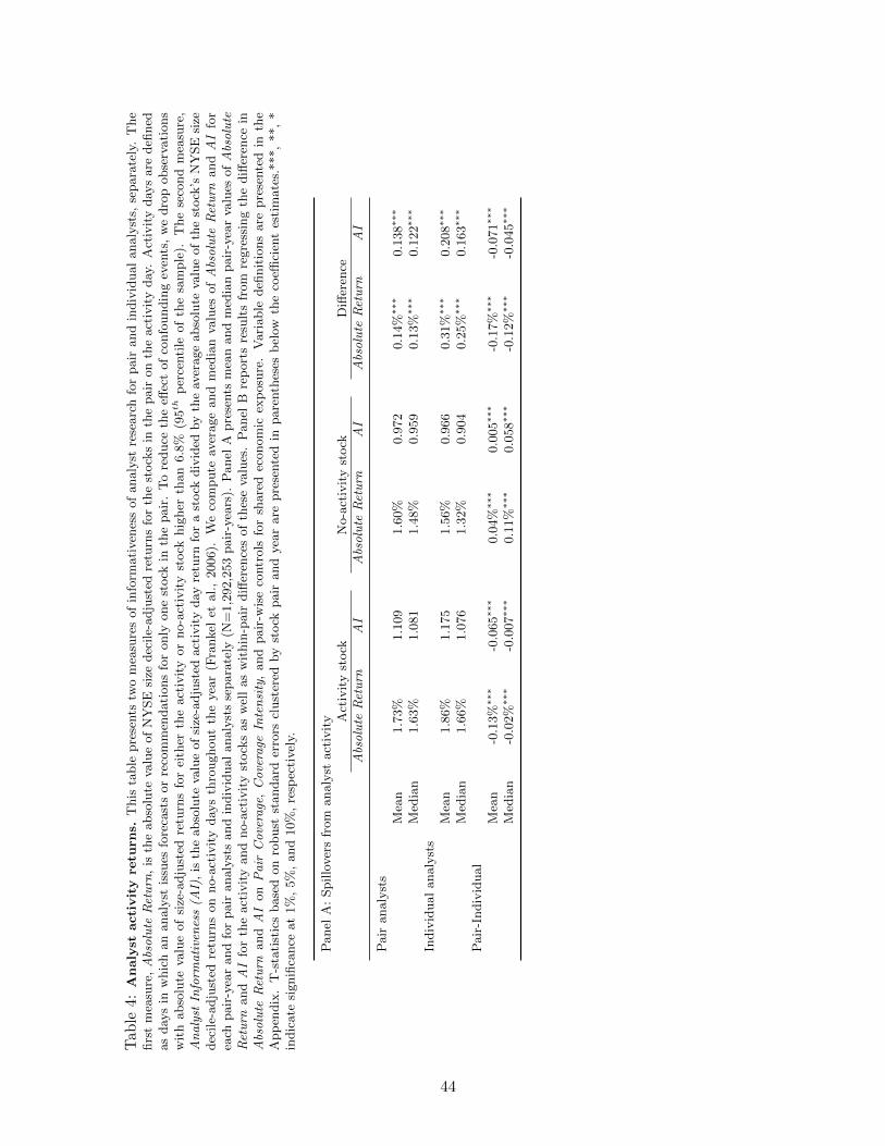
Table

4:A

naly

stacti

vit

yre

turn

s.T

his

table

pre

sents

two

mea

sure

sof

info

rmati

ven

ess

of

analy

stre

searc

hfo

rpair

and

indiv

idual

analy

sts,

separa

tely

.T

he

firs

tm

easu

re,

Abs

olu

teR

etu

rn,

isth

eabso

lute

valu

eof

NY

SE

size

dec

ile-

adju

sted

retu

rns

for

the

stock

sin

the

pair

on

the

act

ivit

yday

.A

ctiv

ity

day

sare

defi

ned

as

day

sin

whic

han

analy

stis

sues

fore

cast

sor

reco

mm

endati

ons

for

only

one

stock

inth

epair

.T

ore

duce

the

effec

tof

confo

undin

gev

ents

,w

edro

pobse

rvati

ons

wit

habso

lute

valu

eof

size

-adju

sted

retu

rns

for

eith

erth

eact

ivit

yor

no-a

ctiv

ity

stock

hig

her

than

6.8

%(9

5th

per

centi

leof

the

sam

ple

).T

he

seco

nd

mea

sure

,A

naly

stIn

form

ati

ven

ess

(AI)

,is

the

abso

lute

valu

eof

size

-adju

sted

act

ivit

yday

retu

rnfo

ra

stock

div

ided

by

the

aver

age

abso

lute

valu

eof

the

stock

’sN

YSE

size

dec

ile-

adju

sted

retu

rns

on

no-a

ctiv

ity

day

sth

roughout

the

yea

r(F

rankel

etal.,

2006).

We

com

pute

aver

age

and

med

ian

valu

esof

Abs

olu

teR

etu

rnand

AI

for

each

pair

-yea

rand

for

pair

analy

sts

and

indiv

idual

analy

sts

separa

tely

(N=

1,2

92,2

53

pair

-yea

rs).

Panel

Apre

sents

mea

nand

med

ian

pair

-yea

rva

lues

of

Abs

olu

teR

etu

rnand

AI

for

the

act

ivit

yand

no-a

ctiv

ity

stock

sas

wel

las

wit

hin

-pair

diff

eren

ces

of

thes

eva

lues

.P

anel

Bre

port

sre

sult

sfr

om

regre

ssin

gth

ediff

eren

cein

Abs

olu

teR

etu

rnand

AI

on

Pair

Co

vera

ge,

Co

vera

geIn

ten

sity

,and

pair

-wis

eco

ntr

ols

for

share

dec

onom

icex

posu

re.

Vari

able

defi

nit

ions

are

pre

sente

din

the

App

endix

.T

-sta

tist

ics

base

don

robust

standard

erro

rscl

ust

ered

by

stock

pair

and

yea

rare

pre

sente

din

pare

nth

eses

bel

owth

eco

effici

ent

esti

mate

s.***,

**,

*in

dic

ate

signifi

cance

at

1%

,5%

,and

10%

,re

spec

tivel

y.

Panel

A:

Spillo

ver

sfr

om

analy

stact

ivit

y Act

ivit

yst

ock

No-a

ctiv

ity

stock

Diff

eren

ceA

bsolu

teR

etu

rnA

IA

bsolu

teR

etu

rnA

IA

bso

lute

Ret

urn

AI

Pair

analy

sts

Mea

n1.7

3%

1.1

09

1.6

0%

0.9

72

0.1

4%∗∗∗

0.1

38∗∗∗

Med

ian

1.6

3%

1.0

81

1.4

8%

0.9

59

0.1

3%∗∗∗

0.1

22∗∗∗

Indiv

idual

analy

sts

Mea

n1.8

6%

1.1

75

1.5

6%

0.9

66

0.3

1%∗∗∗

0.2

08∗∗∗

Med

ian

1.6

6%

1.0

76

1.3

2%

0.9

04

0.2

5%∗∗∗

0.1

63∗∗∗

Pair

-Indiv

idual

Mea

n-0

.13%∗∗∗

-0.0

65∗∗∗

0.0

4%∗∗∗

0.0

05∗∗∗

-0.1

7%∗∗∗

-0.0

71∗∗∗

Med

ian

-0.0

2%∗∗∗

-0.0

07∗∗∗

0.1

1%∗∗∗

0.0

58∗∗∗

-0.1

2%∗∗∗

-0.0

45∗∗∗

44

Panel B: Difference in spillovers from activity by pair analysts and individual analystsDiff Absolute Return Diff AI

(1) (2) (3) (4) (1) (2) (3) (4)

Pair Coverage 0.248∗∗∗ 0.183∗∗∗ 0.181∗∗∗ 0.286∗∗∗ 0.103∗∗∗ 0.095∗∗∗ 0.093∗∗∗ 0.177∗∗∗

(4.83) (3.77) (3.75) (5.82) (4.34) (4.13) (4.11) (6.60)Coverage Intensity -0.013 -0.008 -0.008 -0.004 0.002 0.003 0.003 0.007∗

(-1.33) (-0.87) (-0.83) (-0.39) (0.48) (0.69) (0.70) (1.80)Same Industry -0.048∗∗∗ -0.059∗∗∗ -0.059∗∗∗ -0.050∗∗∗ -0.017∗∗∗ -0.019∗∗∗ -0.019∗∗∗ -0.012∗∗∗

(-5.22) (-6.12) (-6.19) (-5.29) (-4.39) (-4.57) (-4.76) (-2.98)Related Industry -0.024∗∗ -0.024∗∗ -0.024∗∗∗ -0.022∗∗ -0.008∗ -0.008∗ -0.009∗ -0.007

(-2.51) (-2.57) (-2.65) (-2.39) (-1.73) (-1.74) (-1.73) (-1.46)Same Exchange 0.050∗∗∗ 0.032∗∗∗ 0.032∗∗∗ 0.033∗∗∗ -0.005 -0.007∗∗ -0.007∗∗ -0.006∗

(7.77) (5.23) (5.36) (5.44) (-1.40) (-2.18) (-2.12) (-1.70)Same State -0.003 0.000 -0.000 -0.005 0.004 0.004 0.004 -0.001

(-0.48) (0.05) (-0.09) (-1.04) (1.22) (1.34) (1.21) (-0.36)S&P500 Members 0.141∗∗∗ 0.074∗∗∗ 0.074∗∗∗ 0.064∗∗∗ 0.040∗∗∗ 0.031∗∗∗ 0.031∗∗∗ 0.023∗∗∗

(9.33) (5.65) (5.58) (4.67) (5.18) (4.15) (4.10) (3.17)Similar Asset 0.100∗∗∗ 0.101∗∗∗ 0.101∗∗∗ 0.015∗∗∗ 0.015∗∗∗ 0.016∗∗∗

(11.81) (11.72) (11.55) (6.73) (6.79) (6.52)Similar BM -0.005 -0.005 -0.006 0.001 0.001 0.001

(-1.45) (-1.50) (-1.63) (0.59) (0.63) (0.39)Similar Age 0.031∗∗∗ 0.031∗∗∗ 0.031∗∗∗ 0.007∗∗∗ 0.007∗∗∗ 0.006∗∗∗

(6.49) (6.66) (6.36) (2.84) (3.07) (2.72)Similar Leverage 0.002 0.002 0.001 0.002 0.002 0.001

(0.48) (0.42) (0.31) (0.86) (0.79) (0.54)Similar ROA 0.026∗∗∗ 0.026∗∗∗ 0.025∗∗∗ 0.006∗∗ 0.006∗∗ 0.005∗

(5.69) (5.48) (5.23) (2.26) (2.24) (1.89)Similar EPS 0.019∗∗∗ 0.020∗∗∗ 0.021∗∗∗ 0.002 0.002 0.003

(7.24) (7.17) (8.06) (0.90) (1.03) (1.47)Similar Price 0.055∗∗∗ 0.055∗∗∗ 0.055∗∗∗ -0.001 -0.001 -0.001

(9.28) (9.39) (9.12) (-0.50) (-0.59) (-0.63)ROA Correlation 0.005 0.006 0.001 0.001

(1.08) (1.37) (0.24) (0.59)∆ROA Correlation -0.008 -0.009 -0.005 -0.005

(-1.08) (-1.16) (-1.24) (-1.36)EPS Correlation -0.008 -0.009 -0.003 -0.004∗

(-1.49) (-1.61) (-1.45) (-1.73)∆EPS Correlation 0.014∗ 0.015∗∗ 0.004 0.005

(1.91) (2.16) (0.92) (1.28)Diff Experience -0.064∗∗∗ -0.042∗∗∗

(-5.44) (-4.82)Diff Broker Size -0.044∗∗∗ -0.038∗∗∗

(-11.37) (-10.80)Diff Companies 0.057∗∗∗ 0.029∗∗∗

(6.91) (4.34)Diff Forecast Error -1.576∗∗∗ -0.079

(-3.75) (-0.35)Constant -0.195∗∗∗ -0.255∗∗∗ -0.257∗∗∗ -0.303∗∗∗ -0.076∗∗∗ -0.084∗∗∗ -0.085∗∗∗ -0.120∗∗∗

(-6.35) (-7.59) (-7.64) (-9.20) (-4.50) (-4.79) (-4.80) (-6.00)

Adj. R2 0.25% 0.43% 0.43% 0.56% 0.04% 0.05% 0.05% 0.26%N 1,292,253 1,292,253 1,274,571 1,268,872 1,292,253 1,292,253 1,274,571 1,268,872

45

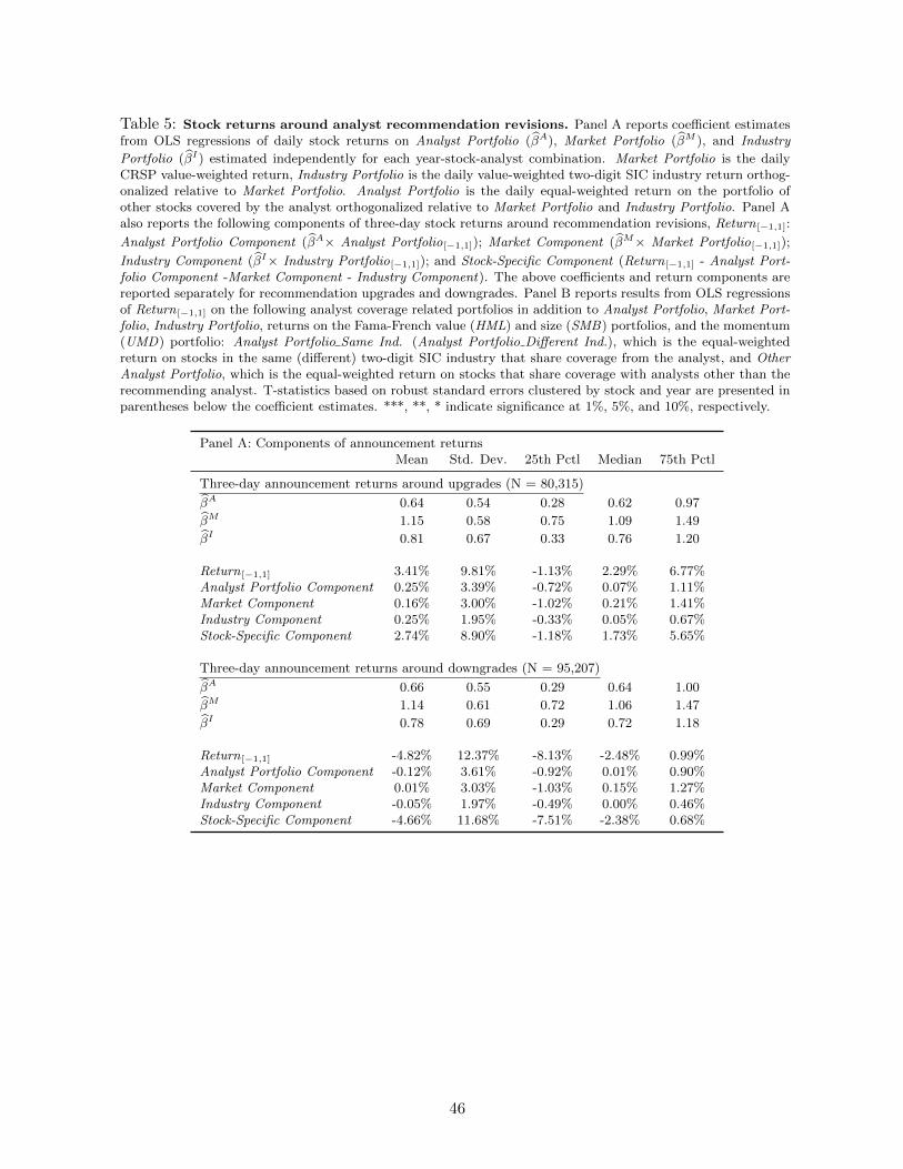
Table 5: Stock returns around analyst recommendation revisions. Panel A reports coefficient estimatesfrom OLS regressions of daily stock returns on Analyst Portfolio (β̂A), Market Portfolio (β̂M ), and Industry

Portfolio (β̂I) estimated independently for each year-stock-analyst combination. Market Portfolio is the dailyCRSP value-weighted return, Industry Portfolio is the daily value-weighted two-digit SIC industry return orthog-onalized relative to Market Portfolio. Analyst Portfolio is the daily equal-weighted return on the portfolio ofother stocks covered by the analyst orthogonalized relative to Market Portfolio and Industry Portfolio. Panel Aalso reports the following components of three-day stock returns around recommendation revisions, Return [−1,1]:

Analyst Portfolio Component (β̂A× Analyst Portfolio[−1,1]); Market Component (β̂M× Market Portfolio[−1,1]);

Industry Component (β̂I× Industry Portfolio[−1,1]); and Stock-Specific Component (Return [−1,1] - Analyst Port-folio Component -Market Component - Industry Component). The above coefficients and return components arereported separately for recommendation upgrades and downgrades. Panel B reports results from OLS regressionsof Return [−1,1] on the following analyst coverage related portfolios in addition to Analyst Portfolio, Market Port-folio, Industry Portfolio, returns on the Fama-French value (HML) and size (SMB) portfolios, and the momentum(UMD) portfolio: Analyst Portfolio Same Ind. (Analyst Portfolio Different Ind.), which is the equal-weightedreturn on stocks in the same (different) two-digit SIC industry that share coverage from the analyst, and OtherAnalyst Portfolio, which is the equal-weighted return on stocks that share coverage with analysts other than therecommending analyst. T-statistics based on robust standard errors clustered by stock and year are presented inparentheses below the coefficient estimates. ***, **, * indicate significance at 1%, 5%, and 10%, respectively.

Panel A: Components of announcement returnsMean Std. Dev. 25th Pctl Median 75th Pctl

Three-day announcement returns around upgrades (N = 80,315)

β̂A 0.64 0.54 0.28 0.62 0.97

β̂M 1.15 0.58 0.75 1.09 1.49

β̂I 0.81 0.67 0.33 0.76 1.20

Return [−1,1] 3.41% 9.81% -1.13% 2.29% 6.77%Analyst Portfolio Component 0.25% 3.39% -0.72% 0.07% 1.11%Market Component 0.16% 3.00% -1.02% 0.21% 1.41%Industry Component 0.25% 1.95% -0.33% 0.05% 0.67%Stock-Specific Component 2.74% 8.90% -1.18% 1.73% 5.65%

Three-day announcement returns around downgrades (N = 95,207)

β̂A 0.66 0.55 0.29 0.64 1.00

β̂M 1.14 0.61 0.72 1.06 1.47

β̂I 0.78 0.69 0.29 0.72 1.18

Return [−1,1] -4.82% 12.37% -8.13% -2.48% 0.99%Analyst Portfolio Component -0.12% 3.61% -0.92% 0.01% 0.90%Market Component 0.01% 3.03% -1.03% 0.15% 1.27%Industry Component -0.05% 1.97% -0.49% 0.00% 0.46%Stock-Specific Component -4.66% 11.68% -7.51% -2.38% 0.68%

46

Panel B: Regressions of announcement returnsThree-day announcement returns

(1) (2) (3) (4)

Analyst Portfolio 1.112∗∗∗ 1.109∗∗∗ 0.742∗∗∗

(25.31) (26.56) (18.87)Analyst Portfolio Same Ind. 0.686∗∗∗

(16.34)Analyst Portfolio Different Ind. 0.288∗∗∗

(9.82)Other Analyst Portfolio 0.581∗∗∗

(8.29)Market Portfolio 1.193∗∗∗ 1.175∗∗∗ 1.167∗∗∗ 1.203∗∗∗

(21.36) (19.20) (18.45) (19.58)Industry Portfolio 1.212∗∗∗ 1.213∗∗∗ 1.216∗∗∗ 1.285∗∗∗

(20.63) (20.78) (21.39) (23.46)SMB -0.005 -0.025 -0.003

(-0.19) (-0.86) (-0.10)HML -0.037∗∗ -0.038∗∗ -0.043∗∗

(-2.32) (-2.37) (-2.51)UMD -0.020∗∗∗ -0.018∗∗ -0.021∗∗∗

(-2.71) (-2.57) (-2.81)Constant -0.013∗∗∗ -0.012∗∗∗ -0.012∗∗∗ -0.012∗∗∗

(-5.53) (-5.48) (-5.50) (-5.43)

t-stat (An. Port. = Other An. Port.) 1.79t-stat (An. Port. Same Ind. = An. Port. Diff Ind.) 6.99

Adj. R2 12.6% 12.6% 13.0% 13.1%N 175,522 175,522 173,623 157,070

47

Table 6: Pair coverage and return correlation. This table reports results from OLS regressions ofCorrelation on Pair Coverage and a set of pair-wise controls. Variable definitions are presented in the Appendix.T-statistics based on robust standard errors clustered by stock pair and year are presented in parentheses belowthe coefficient estimates. ***, **, * indicate significance at 1%, 5%, and 10%, respectively.

CorrelationPair Universe Sample Pairs

(1) (2) (3) (4) (5) (6)

Pair Coverage 0.505 ∗∗∗ 0.493∗∗∗ 0.231∗∗∗ 0.213∗∗∗ 0.201∗∗∗ 0.218∗∗∗

(17.93) (17.66) (10.17) (9.93) (9.34) (9.99)Coverage Intensity 0.048 ∗∗∗ 0.048 ∗∗∗ 0.046∗∗∗ 0.046∗∗∗ 0.046∗∗∗ 0.046∗∗∗

(9.81) (9.91) (6.49) (6.33) (6.39) (6.47)Same Industry 0.019 ∗∗∗ 0.017 ∗∗∗ 0.059∗∗∗ 0.053∗∗∗ 0.051∗∗∗ 0.048∗∗∗

(3.99) (3.63) (13.89) (14.19) (12.97) (12.14)Related Industry 0.000 -0.001 0.026∗∗∗ 0.025∗∗∗ 0.022∗∗∗ 0.022∗∗∗

(-0.12) (-0.27) (5.43) (5.39) (5.06) (5.01)Same Exchange 0.030 ∗∗∗ 0.028 ∗∗∗ 0.050∗∗∗ 0.045∗∗∗ 0.044∗∗∗ 0.044∗∗∗

(7.81) (6.92) (10.83) (8.83) (8.98) (8.60)Same State 0.005 ∗∗ 0.004 ∗∗ 0.019∗∗∗ 0.019∗∗∗ 0.016∗∗∗ 0.018∗∗∗

(2.39) (2.19) (3.84) (3.91) (3.37) (3.61)S&P500 Members 0.063 ∗∗∗ 0.056∗∗∗ 0.080∗∗∗ 0.066∗∗∗ 0.066∗∗∗ 0.066∗∗∗

(6.61) (5.70) (8.54) (6.35) (6.40) (6.54)Similar Asset 0.008 ∗∗∗ 0.017∗∗∗ 0.017∗∗∗ 0.017∗∗∗

(7.22) (7.66) (7.64) (7.58)Similar BM 0.003 ∗∗∗ 0.006∗∗ 0.006∗∗ 0.006∗∗

(6.55) (2.23) (1.96) (2.06)Similar Age 0.002∗∗∗ 0.007∗∗∗ 0.008∗∗∗ 0.008∗∗∗

(3.76) (3.85) (4.09) (4.17)Similar Leverage 0.002∗∗∗ 0.011∗∗∗ 0.011∗∗∗ 0.011∗∗∗

(2.60) (3.92) (3.55) (3.54)Similar ROA 0.003 ∗∗∗ 0.011∗∗∗ 0.008∗∗ 0.008∗∗

(5.50) (3.04) (2.30) (2.34)Similar EPS 0.004 ∗∗∗ 0.007∗ 0.004 0.004

(5.15) (1.66) (1.03) (0.99)Similar Price 0.009 ∗∗∗ 0.016∗∗∗ 0.016∗∗∗ 0.016∗∗∗

(17.44) (10.69) (11.16) (11.33)ROA Correlation 0.036∗∗∗ 0.036∗∗∗

(4.07) (4.10)∆ROA Correlation 0.017∗∗∗ 0.017∗∗∗

(5.79) (5.78)EPS Correlation 0.007 0.007

(1.35) (1.37)∆EPS Correlation 0.027∗∗∗ 0.026∗∗∗

(3.30) (3.29)Diff Experience -0.004

(-1.64)Diff Broker Size 0.011∗∗∗

(4.66)Diff Companies 0.002

(0.42)Diff Forecast Error -0.492∗∗∗

(-2.86)Constant 0.101 ∗∗∗ 0.094∗∗∗ 0.117∗∗∗ 0.098∗∗∗ 0.096∗∗∗ 0.100∗∗∗

(5.16) (4.82) (3.57) (2.80) (2.82) (2.83)

Adj. R2 6.3% 6.5% 10.5% 11.3% 13.5% 14.1%N 91,561,175 91,561,175 1,489,895 1,489,895 1,470,060 1,460,819

48

Table 7: Return correlation and forecasts. This table reports results from OLS regressions of Correlationon Pair Forecast Correlation, Individual Forecast Correlation and a set of pair-wise controls. Variable definitionsare presented in the Appendix. T-statistics based on robust standard errors clustered by stock pair and year arepresented in parentheses below the coefficient estimates. ***, **, * indicate significance at 1%, 5%, and 10%,respectively.

Correlation(1) (2) (3) (4)

Pair Forecast Correlation 0.014∗∗∗ 0.013∗∗∗ 0.009∗∗∗ 0.009∗∗∗

(11.28) (9.78) (9.06) (8.89)Individual Forecast Correlation 0.015∗∗∗ 0.014∗∗∗ 0.009∗∗∗ 0.009∗∗∗

(4.08) (3.77) (2.78) (2.85)Coverage Intensity 0.030∗∗∗ 0.031∗∗∗ 0.032∗∗∗ 0.032∗∗∗

(4.38) (4.32) (4.56) (4.51)Same Industry 0.061∗∗∗ 0.052∗∗∗ 0.049∗∗∗ 0.046∗∗∗

(11.08) (12.68) (11.43) (10.64)Related Industry 0.026∗∗∗ 0.025∗∗∗ 0.021∗∗∗ 0.021∗∗∗

(5.42) (5.31) (4.91) (4.82)Same Exchange 0.050∗∗∗ 0.043∗∗∗ 0.042∗∗∗ 0.041∗∗∗

(7.94) (6.61) (6.74) (6.56)Same State 0.027∗∗∗ 0.027∗∗∗ 0.023∗∗∗ 0.024∗∗∗

(4.73) (4.82) (4.32) (4.54)S&P500 Members 0.113∗∗∗ 0.092∗∗∗ 0.090∗∗∗ 0.090∗∗∗

(15.53) (11.61) (11.52) (11.56)Similar Asset 0.027∗∗∗ 0.027∗∗∗ 0.026∗∗∗

(9.02) (8.78) (8.57)Similar BM 0.007∗ 0.006 0.006∗

(1.80) (1.62) (1.66)Similar Age 0.009∗∗∗ 0.010∗∗∗ 0.010∗∗∗

(4.01) (4.58) (4.61)Similar Leverage 0.017∗∗∗ 0.016∗∗∗ 0.016∗∗∗

(4.53) (4.14) (4.18)Similar ROA 0.014∗∗∗ 0.011∗∗∗ 0.012∗∗∗

(3.75) (2.87) (2.94)Similar EPS 0.004 0.002 0.001

(0.83) (0.33) (0.30)Similar Price 0.019∗∗∗ 0.018∗∗∗ 0.018∗∗∗

(6.81) (7.32) (7.39)ROA Correlation 0.045∗∗∗ 0.044∗∗∗

(4.55) (4.59)∆ROA Correlation 0.022∗∗∗ 0.022∗∗∗

(6.87) (6.97)EPS Correlation 0.003 0.003

(0.42) (0.45)∆EPS Correlation 0.036∗∗∗ 0.035∗∗∗

(4.11) (4.10)Diff Experience -0.007∗

(-1.73)Diff Broker Size 0.016∗∗∗

(6.85)Diff Companies -0.002

(-0.36)Diff Forecast Error -1.178∗∗∗

(-5.98)Constant 0.187∗∗∗ 0.160∗∗∗ 0.154∗∗∗ 0.161∗∗∗

(5.28) (4.10) (4.11) (4.22)

Adj. R2 9.8% 11.1% 14.1% 14.8%N 688,755 688,755 683,084 682,458

49

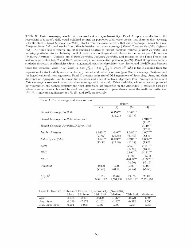
Table 8: Pair coverage, stock returns and return synchronicity. Panel A reports results from OLSregressions of a stock’s daily equal-weighted returns on portfolios of all other stocks that share analyst coveragewith the stock (Shared Coverage Portfolio), stocks from the same industry that share coverage (Shared CoveragePortfolio Same Ind.), and stocks from other industries that share coverage (Shared Coverage Portfolio DifferentInd.). All three sets of returns are orthogonalized relative to market portfolio returns (Market Portfolio) andindustry portfolio returns. Industry portfolio returns are orthogonalized relative to the market portfolio returns(Industry Portfolio). Controls are Market Portfolio, Industry Portfolio, and returns on the Fama-French sizeand value portfolios (SMB, and HML, respectively), and momentum portfolio (UMD). Panel B reports summarystatistics for return synchronicity (Sync), augmented return synchronicity (Aug. Sync), and the difference between

these two variables. Sync (Aug. Sync) is Log( R2

1−R2 ) ( Log(R2

S

1−R2S

)), where R2 (R2S) is the R-squared from the

regression of a stock’s daily return on the daily market and industry returns (plus Shared Coverage Portfolio) andthe lagged values of these regressors. Panel C presents estimates of OLS regressions of Sync, Aug. Sync, and theirdifference on Aggregate Pair Coverage for the stock and a set of controls. Aggregate Pair Coverage is the sum ofPair Coverage across stock pairs that share coverage with the stock. Other variables, whose names are precededby “Aggregate”, are defined similarly and their definitions are presented in the Appendix. T-statistics based onrobust standard errors clustered by stock and year are presented in parentheses below the coefficient estimates.***, **, * indicate significance at 1%, 5%, and 10%, respectively.

Panel A: Pair coverage and stock returnsReturn

(1) (2) (3) (4)

Shared Coverage Portfolio 0.450∗∗∗ 0.384∗∗∗

(15.23) (13.77)Shared Coverage Portfolio Same Ind. 0.218∗∗∗

(11.05)Shared Coverage Portfolio Different Ind. 0.110∗∗∗

(17.66)Market Portfolio 1.040∗∗∗ 1.040∗∗∗ 1.044∗∗∗ 1.067∗∗∗

(21.62) (21.65) (69.49) (82.79)Industry Portfolio 0.614∗∗∗ 0.613∗∗∗ 0.594∗∗∗ 0.655∗∗∗

(13.50) (13.48) (13.18) (15.00)SMB 0.459∗∗∗ 0.461∗∗∗

(14.99) (16.50)HML 0.196∗∗∗ 0.171∗∗∗

(7.09) (6.04)UMD -0.083∗∗∗ -0.090∗∗∗

(-4.50) (-5.19)Constant -0.000 -0.000 -0.000∗∗ -0.000∗∗∗

(-0.40) (-0.50) (-2.45) (-3.50)

Adj. R2 16.4% 18.3% 19.0% 20.0%N 9,591,192 9,591,192 9,591,192 7,571,993

Panel B: Descriptive statistics for return synchronicity (N=49,467)Mean Minimum 25th Pctl Median 75th Pctl Maximum

Sync -1.503 -8.440 -2.329 -1.377 -0.570 4.595Aug. Sync -1.299 -7.373 -2.162 -1.207 -0.372 4.595Aug. Sync-Sync 0.204 0.000 0.027 0.099 0.253 5.956

50

Panel C: Aggregate pair coverage and stock return synchronicitySync Aug. Sync Aug. Sync - Sync

(1) (2) (3) (4) (5) (6) (7) (8) (9)

Agg. Pair Coverage 0.042∗∗∗ 0.044∗∗∗ 0.059∗∗∗ 0.066∗∗∗ 0.017∗∗∗ 0.022∗∗∗

(3.60) (3.80) (4.96) (6.17) (6.91) (7.86)Log(Coverage) 0.074∗∗ -0.027 -0.138∗∗∗ 0.098∗∗∗ -0.044 -0.146∗∗∗ 0.024∗∗∗ -0.017∗∗ -0.008

(2.36) (-0.71) (-3.39) (3.45) (-1.19) (-3.83) (2.92) (-2.55) (-1.10)Log (Market Cap) 0.236∗∗∗ 0.227∗∗∗ 0.297∗∗∗ 0.268∗∗∗ 0.255∗∗∗ 0.324∗∗∗ 0.032∗∗∗ 0.028∗∗∗ 0.027∗∗∗

(8.93) (8.35) (11.75) (11.43) (10.54) (14.17) (5.31) (4.88) (6.83)BM 0.594∗∗∗ 0.547∗∗∗ 0.470∗∗∗ 0.655∗∗∗ 0.589∗∗∗ 0.508∗∗∗ 0.061∗∗∗ 0.042∗∗∗ 0.038∗∗∗

(3.64) (3.40) (3.12) (4.17) (3.81) (3.61) (4.80) (3.09) (2.58)Log (Volume) 0.227∗∗∗ 0.238∗∗∗ 0.254∗∗∗ 0.213∗∗∗ 0.229∗∗∗ 0.243∗∗∗ -0.014∗∗ -0.009 -0.011

(4.96) (5.32) (6.30) (4.85) (5.34) (6.46) (-2.17) (-1.47) (-1.63)Agg. Same Industry 0.003∗∗ 0.001∗ -0.001∗∗

(2.28) (1.70) (-2.26)Agg. Related Industry -0.002∗ -0.003∗∗∗ -0.001∗∗∗

(-1.71) (-3.52) (-2.76)Agg. Same Exchange 0.006∗∗∗ 0.006∗∗∗ 0.001∗∗

(4.00) (4.66) (2.17)Agg. Same State -0.002∗∗∗ 0.000 0.003∗∗∗

(-2.73) (0.47) (4.67)Agg. S&P500 Members -0.017∗∗∗ -0.017∗∗∗ -0.000

(-7.14) (-7.76) (-0.26)Agg. Sim. Asset -0.007∗∗∗ -0.007∗∗∗ -0.000

(-5.25) (-5.22) (-0.28)Agg. Sim. BM -0.003∗ -0.002∗∗ 0.000

(-1.67) (-2.08) (0.22)Agg. Sim. Age 0.001 0.001 0.001

(0.73) (1.38) (1.06)Agg. Sim. Leverage 0.003∗∗ 0.003∗∗ -0.000

(2.48) (2.09) (-1.45)Agg. Sim. ROA 0.003∗∗ 0.003∗∗∗ 0.000

(2.23) (2.58) (0.55)Agg. Sim. EPS 0.001 0.001 -0.001

(0.78) (0.29) (-1.57)Agg. Sim. Price -0.000 -0.000 -0.000

(-0.04) (-0.09) (-0.09)Agg. ROA Corr. 0.009∗∗∗ 0.010∗∗∗ 0.001∗∗∗

(6.12) (6.81) (2.83)Agg. ∆ROA Corr. 0.008∗∗∗ 0.006∗∗∗ -0.002∗∗∗

(3.43) (2.67) (-2.88)Agg. EPS Corr. -0.002 -0.001 0.001∗

(-1.03) (-0.60) (1.94)Agg. ∆EPS Corr. 0.013∗∗∗ 0.013∗∗∗ 0.000

(5.65) (5.59) (0.15)Agg. Diff Experience -0.004∗∗∗ -0.002∗∗ 0.001∗∗∗

(-3.11) (-2.17) (3.89)Agg. Diff Broker Size 0.000 0.001∗∗ 0.001∗∗∗

(0.88) (2.27) (3.93)Agg. Diff Companies -0.012∗∗∗ -0.013∗∗∗ -0.001∗

(-5.02) (-5.51) (-1.93)Agg. Diff Forecast Err. -0.160 -0.130 0.029

(-1.49) (-1.28) (1.12)Constant -4.502∗∗∗ -4.521∗∗∗ -4.901∗∗∗ -4.540∗∗∗ -4.568∗∗∗ -4.951∗∗∗ -0.038 -0.046 -0.050∗

(-18.81) (-18.95) (-21.44) (-20.99) (-21.15) (-23.50) (-1.22) (-1.47) (-1.78)

Adj. R2 49,467 49,467 48,500 49,467 49,467 48,500 49,467 49,467 48,500N 36.1% 36.6% 44.10% 40.6% 41.5% 49.40% 3.5% 4.9% 7.20%

51

sell-side analyst research and stock comovement rebello xu (2013).pdf · sell-side analyst research...

Documents