SELF-LOCALIZATION OF HUMANOID ROBOT

IN A SOCCER FIELD

TIAN BO

A THESIS SUBMITTED

FOR THE DEGREE OF MASTER OF ENGINEERING

DEPARTMENT OF MECHANICAL ENGINEERING

NATIONAL UNIVERSITY OF SINGAPORE

2010

i

ACKNOWLEDGMENTS

I would like to express my appreciation to the my supervisor, Prof. Chew Chee Meng, for

the opportunity to work on the RoboCup project and the chance to gain valuable

experience from the prestigious RoboCup competitions, as well as for his patient

guidance in the various aspects of the project.

Next, the author wishes to thank the following people for their assistance during the

course of this project:

1) The members of Team ROPE, Samuel, Chongyou, Chuen Leong, Xiyang,

Ruizhong, Renjun, Junwen, Bingquan, Wenhao, Yuanwei, Jiayi, Jia Cheng, Soo

Theng, Reyhan, Jason and all the other team members, for their friendship and

untiring efforts towards the team’s cause. Their dedication and unwavering spirit

was motivating and inspiring.

2) Mr. Tomasz Marek Lubecki for his insights and suggestions with regards to many

aspects of the project.

3) Mr. Huang Wei-wei, Mr Fu Yong and Mr Zheng Yu, for their guidance and

suggestions on advanced algorithms applied on the robots.

4) The professors, technicians, staff and students in the Control and Mechatronics

Laboratories 1 and 2, for their unwavering technical support and advice.

Last, I want to thank my parents. This thesis is dedicated to them.

ii

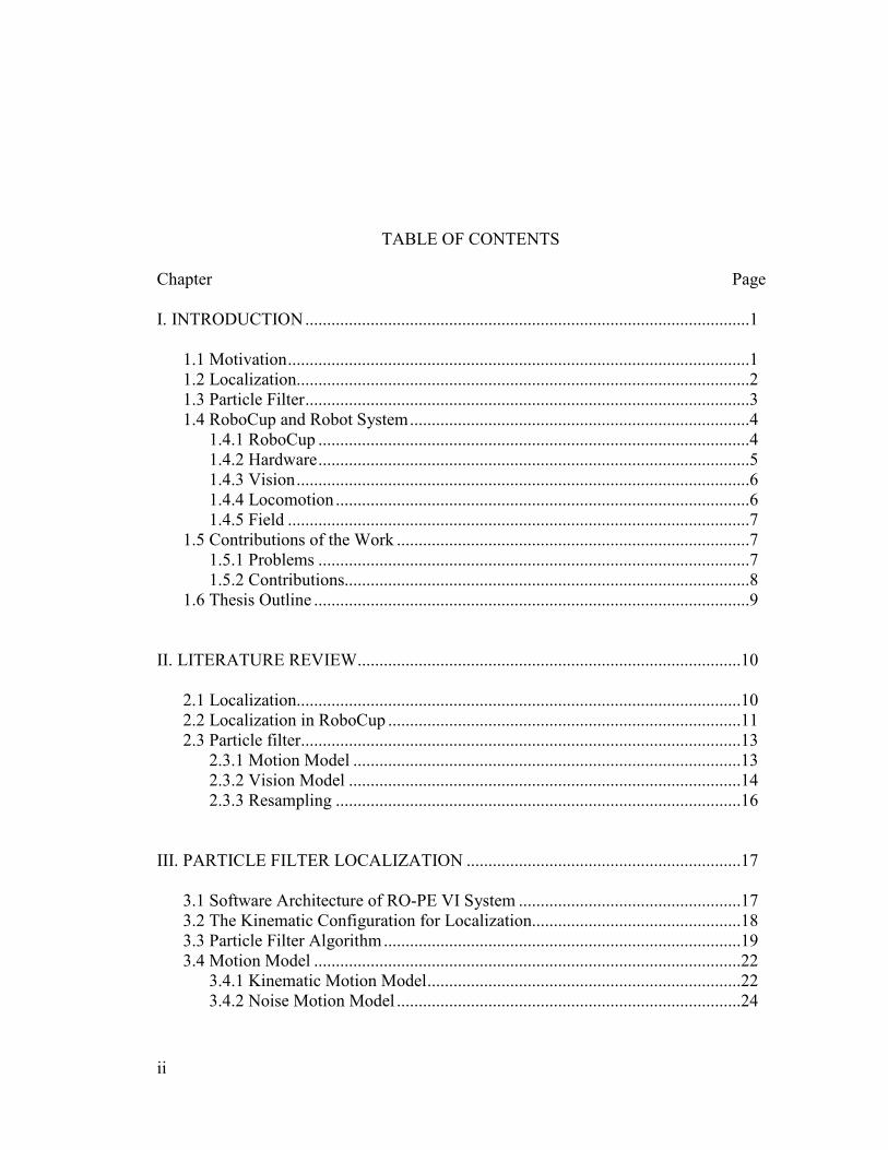
TABLE OF CONTENTS

Chapter Page

I. INTRODUCTION ......................................................................................................1

1.1 Motivation ..........................................................................................................1

1.2 Localization........................................................................................................2

1.3 Particle Filter ......................................................................................................3

1.4 RoboCup and Robot System ..............................................................................4

1.4.1 RoboCup ...................................................................................................4

1.4.2 Hardware ...................................................................................................5

1.4.3 Vision ........................................................................................................6

1.4.4 Locomotion ...............................................................................................6

1.4.5 Field ..........................................................................................................7

1.5 Contributions of the Work .................................................................................7

1.5.1 Problems ...................................................................................................7

1.5.2 Contributions.............................................................................................8

1.6 Thesis Outline ....................................................................................................9

II. LITERATURE REVIEW ........................................................................................10

2.1 Localization......................................................................................................10

2.2 Localization in RoboCup .................................................................................11

2.3 Particle filter.....................................................................................................13

2.3.1 Motion Model .........................................................................................13

2.3.2 Vision Model ..........................................................................................14

2.3.3 Resampling .............................................................................................16

III. PARTICLE FILTER LOCALIZATION ...............................................................17

3.1 Software Architecture of RO-PE VI System ...................................................17

3.2 The Kinematic Configuration for Localization................................................18

3.3 Particle Filter Algorithm ..................................................................................19

3.4 Motion Model ..................................................................................................22

3.4.1 Kinematic Motion Model ........................................................................22

3.4.2 Noise Motion Model ...............................................................................24

iii

Chapter Page

3.5 Vision Model ...................................................................................................25

3.5.1 The Projection Model of Fisheye Lens ...................................................25

3.5.2 Robot Perception .....................................................................................26

3.5.3 Update .....................................................................................................29

IV. SIMULATION ......................................................................................................31

4.1 The Simulation Algorithm ...............................................................................31

4.1.1 The Particle Reset Algorithm..................................................................32

4.1.2 The Switching Particle Filter Algorithm.................................................33

4.1.3 Calculation of the Robot Pose.................................................................35

4.2 Simulation Result of the Conventional Particle Filter

with Particle Reset Algorithm ................................................................................36

4.2.1 Global Localization .................................................................................36

4.2.2 Position Tracking ....................................................................................38

4.2.3 Kidnapped Problem ................................................................................40

4.3 The Simulation of the Switching Particle Filter Algorithm .............................43

4.4 Conclusion .......................................................................................................45

V. IMPLEMENTATIONS ..........................................................................................46

5.1 Introduction ......................................................................................................46

5.2 Experiment for Motion Model and Vision Model ...........................................47

5.2.1 Experiment for Motion Model ................................................................48

5.2.2 Experiment for Vision Model .................................................................49

5.3 Localization Experiment and the Evaluation ...................................................51

5.3.1 Improvement on Transplanting the Program to an Onboard PC 104 .....52

5.3.2 Evaluation of the Particle Filter Localization Algorithm Onboard ........54

5.4 Future Work .....................................................................................................55

VI. CONCLUSION.....................................................................................................56

REFERENCES ............................................................................................................58

APPENDICES .............................................................................................................60

iv

SUMMARY

RoboCup is an annual international robotics competition that encourages the research and

development of artificial intelligence and robotics. This thesis presents the algorithm

developed for self-localization of small-size humanoid robots, RO-PE (RObot for

Personal Entertainment) series, which participate in RoboCup Soccer Humanoid League

(Kid-Size).

Localization is the most fundamental problem to providing a mobile robot with

autonomous capabilities. The problem of robot localization has been studied by many

researchers in the past decades. In recent years, many researchers adopt the particle filter

algorithm for localization problem.

In this thesis, we implement the particle filter on our humanoid robot to achieve self-

localization. The algorithm is optimized for our system. We use robot kinematic to

develop the motion model. The vision model is also built based on the physical

characteristics of the onboard camera. We simulate the particle filter algorithm in

MatLab™ to validate the effectiveness of the algorithm and develop a new switching

particle filter algorithm to perform the localization. To further illustrate the effectiveness

of the algorithm, we implement the algorithm on our robot to realize self-positioning

capability.

v

LIST OF TABLES

Table Page

5-1: Pole position in the image, according to different angles and distances ...........50

5-2 Relationship between the pole distance and the width of the pole in image ......51

vi

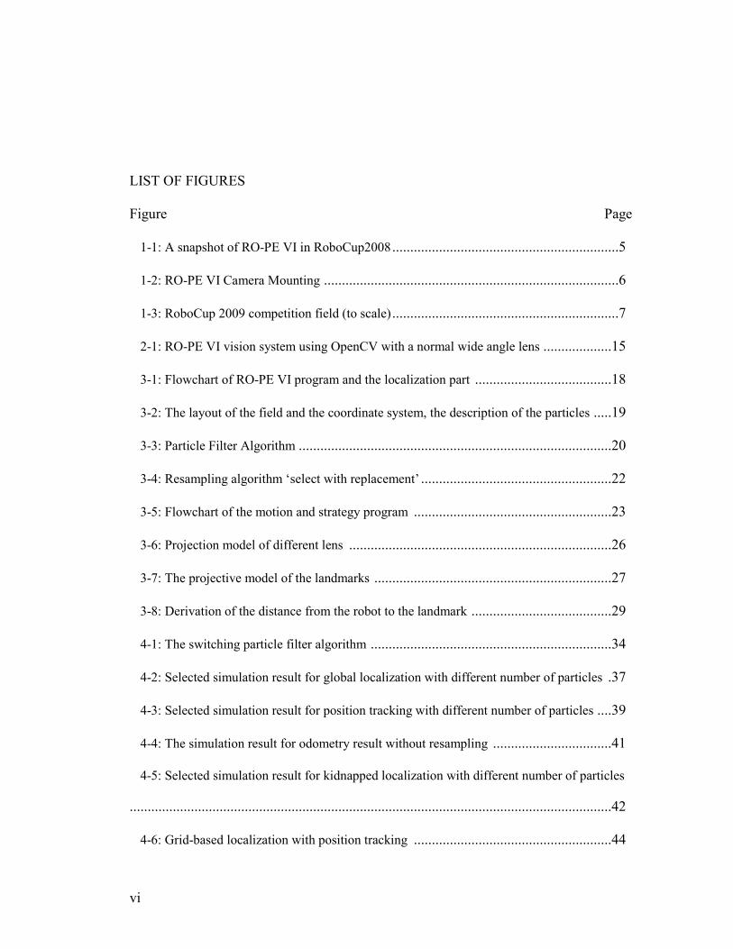
LIST OF FIGURES

Figure Page

1-1: A snapshot of RO-PE VI in RoboCup2008 ...............................................................5

1-2: RO-PE VI Camera Mounting ..................................................................................6

1-3: RoboCup 2009 competition field (to scale) ...............................................................7

2-1: RO-PE VI vision system using OpenCV with a normal wide angle lens ...................15

3-1: Flowchart of RO-PE VI program and the localization part ......................................18

3-2: The layout of the field and the coordinate system, the description of the particles .....19

3-3: Particle Filter Algorithm .......................................................................................20

3-4: Resampling algorithm ‘select with replacement’ .....................................................22

3-5: Flowchart of the motion and strategy program .......................................................23

3-6: Projection model of different lens .........................................................................26

3-7: The projective model of the landmarks ..................................................................27

3-8: Derivation of the distance from the robot to the landmark .......................................29

4-1: The switching particle filter algorithm ...................................................................34

4-2: Selected simulation result for global localization with different number of particles .37

4-3: Selected simulation result for position tracking with different number of particles ....39

4-4: The simulation result for odometry result without resampling .................................41

4-5: Selected simulation result for kidnapped localization with different number of particles

......................................................................................................................................42

4-6: Grid-based localization with position tracking .......................................................44

vii

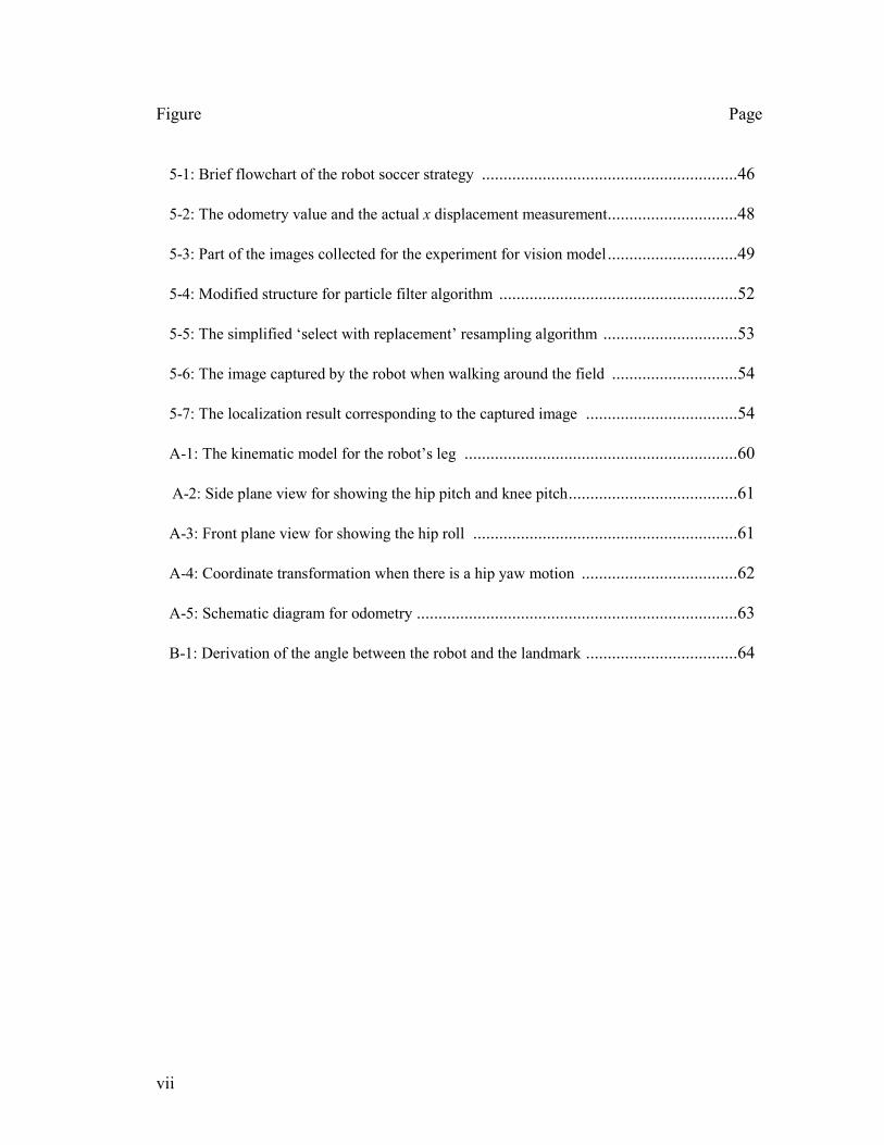
Figure Page

5-1: Brief flowchart of the robot soccer strategy ...........................................................46

5-2: The odometry value and the actual x displacement measurement ..............................48

5-3: Part of the images collected for the experiment for vision model ..............................49

5-4: Modified structure for particle filter algorithm .......................................................52

5-5: The simplified ‘select with replacement’ resampling algorithm ...............................53

5-6: The image captured by the robot when walking around the field .............................54

5-7: The localization result corresponding to the captured image ...................................54

A-1: The kinematic model for the robot’s leg ...............................................................60

A-2: Side plane view for showing the hip pitch and knee pitch .......................................61

A-3: Front plane view for showing the hip roll .............................................................61

A-4: Coordinate transformation when there is a hip yaw motion ....................................62

A-5: Schematic diagram for odometry ..........................................................................63

B-1: Derivation of the angle between the robot and the landmark ...................................64

1

CHAPTER I

INTRODUCTION

This thesis presents the algorithm developed for self-localization of small-size humanoid

robots, RO-PE (RObot for Personal Entertainment) series, which participate in RoboCup

Soccer Humanoid League (Kid-Size). In particular, we focus on the implementation of

the particle filter localization algorithm for the robot RO-PE VI. We developed the

motion model and vision model for the robot, and also improved the computational

efficiency of the particle filter algorithm.

1.1 Motivation

In soccer games, one successful team must not only have talented players but also an

experienced coach who can choose the proper strategy and formation for the team. That

means a good player must be skillful with the ball and aware of his position on the field.

It is the same for a robot soccer player. Our team has spent most of our efforts on

improving the motion and vision ability of the robots. From 2008, the number of the

robots on each side increased from two to three. Therefore, there are more and more

cooperation between the robot players and they have more specific roles. This prompts

more teams to develop self-localization ability for humanoid robot players.

2

1.2 Localization

The localization in RoboCup is the problem of determining the position and heading

(pose) of a robot on the field. Thrun and Fox proposed taxonomy of localization

problems [1, 2]. They divide the localization problems according to the relationship

between the robots and the environment, and the initial knowledge of the position known

by the robot.

The simplest case is position tracking. The initial position of the robot is known, and the

localization will estimate the current location based upon the known or estimated motion.

It can be considered as the dead reckoning problem, which is the position estimation in

the studies of navigation. A more difficult case is global localization problem, where the

initial pose of the robot is not known, but the robot has to determine its position from

scratch. Another case named kidnapped robot problem is even more difficult. The robot

will be teleported without telling it. It is often used to test the ability of the robot to

recover from localization failures.

The problem we discussed in this work is kidnapped robot problem. Other than the

displacement of the robot, the changing environmental elements also have substantial

impact on the localization. Dynamic environments consist of objects whose location or

configuration changes over time. RoboCup soccer game is a highly dynamic

environment. During the game, there are referees, robot handlers, and all the robot

players moving in the field. All these uncertain factors may block the robot from seeing

3

the landmarks. Obviously, the localization in dynamic environments is more difficult

than localization in static ones.

To tackle all these problems in localization, the particle filter is adopted by most of the

researchers in the field of robotics. Particle filters, also known as sequential Monte Carlo

methods (SMC), are sophisticated model estimation techniques [3]. It is an alternative

nonparametric implementation of the Bayes filter. In contrast to other algorithms used in

robotic localization, particle filters can approximate various probability distributions of

the posterior state. Though particle filter always requires hundreds of particles to cover

the domain space, it has been proved [4] that the particle filter can be realized using less

than one hundred particles in RoboCup scenario. This result will enable the particle filter

to be executed in real time.

The self-localization problem was introduced into RoboCup when the middle size league

(MSL) started. In MSL, the players are mid-sized wheeled robots with all the sensors on

board. Later in the Standard Platform League (Four-Legged Robot League using Sony

Aibo, SPL) and the Humanoid League, a number of teams have employed the particle

filters to achieve self-localization.

1.3 Particle Filter

The particle filter is an alternative nonparametric implementation of the Bayes filter. The

main objective of particle filtering is to "track" a variable of interest as it evolves over

time. The basis of the method is to construct a sample-based representation of the entire

4

probability density function (pdf). A series of actions are taken, each one modifying the

state of the variable of interest according to some model. Moreover at certain times, an

observation arrives that constrains the state of the variable of interest at that time.

Multiple copies (particles) of the variable of interest are used, each one associated with a

weight that signifies the quality of that specific particle. An estimate of the variable of

interest is obtained by the weighted sum of all the particles.

The particle filter algorithm is recursive in nature and operates in two phases: prediction

and update. After each action, each particle is modified according to the existing model

(motion model, the prediction stage), including the addition of random noise in order to

simulate the effect of noise on the variable of interest. Then, each particle's weight is re-

evaluated based on the latest sensory information available (sensor model, the update

stage). At times, the particles with (infinitesimally) small weights are eliminated, a

process called resampling. We will give a detailed description of the algorithm in

Chapter 3.

1.4 RoboCup and Robot System

In the rest of this chapter, a brief introduction of RoboCup is first provided, followed by

the hardware, vision and locomotion system of the robot. There are also the description of

the field and challenges faced.

1.4.1 RoboCup

5

RoboCup is a scientific initiative to promote the development of robotics and artificial

intelligence. Since the first competition in 1996, teams from around the world meet

annually to compete against each other and evaluate the state of the art in robot soccer.

The key feature of the games in RoboCup is that the robots are not remotely controlled by

a human operator, and have to be fully autonomous. The ultimate goal of RoboCup is to

develop a team of fully autonomous humanoid robot that can win the human world soccer

champion team by 2050. RoboCup humanoid league started in 2002, and is the most

challenging league among all the categories.

1.4.2 Hardware

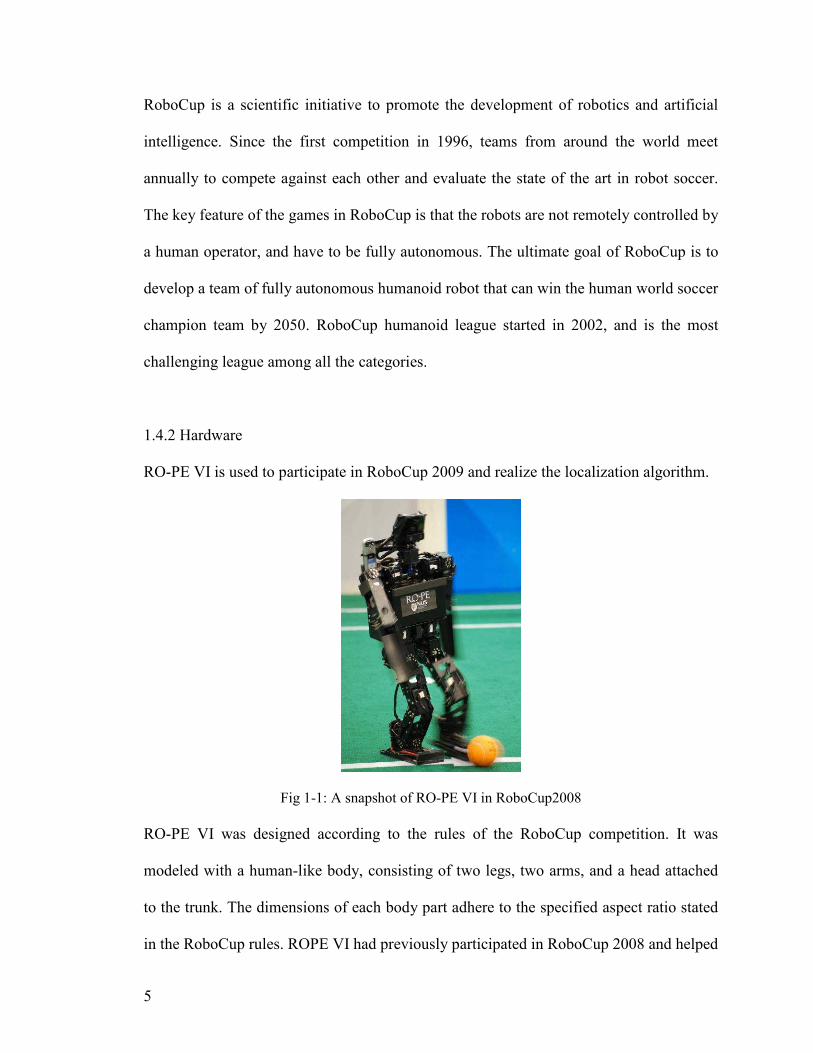
RO-PE VI is used to participate in RoboCup 2009 and realize the localization algorithm.

Fig 1-1: A snapshot of RO-PE VI in RoboCup2008

RO-PE VI was designed according to the rules of the RoboCup competition. It was

modeled with a human-like body, consisting of two legs, two arms, and a head attached

to the trunk. The dimensions of each body part adhere to the specified aspect ratio stated

in the RoboCup rules. ROPE VI had previously participated in RoboCup 2008 and helped

6

the team win fourth place in Humanoid League Kid-size Game. The robot is 57cm high

and weighs 3kg [5].

1.4.3 Vision

Two A4Tech USB webcams are mounted on the robot head with pan motion. The main

camera is equipped with Sunex DSL215A S-mount miniature fisheye angle lens that

provides wide 123˚ horizontal and 92˚ vertical angle of view. The subsidiary camera with

pin-hole lens is mainly used for locating ball at far location. The cameras capture QVGA

images with a resolution of 320x240 at a frame rate of 25 fps. The robot subsequently

processes the images at a frequency of 8 fps [6]. The robot can only acquire image from

one of cameras at any instance due to the USB bandwidth.

Fig 1-2: RO-PE VI Camera Mounting

1.4.4 Locomotion

The locomotion used in our tests was first developed by Ma [7], and improved by Li [8].

Due to the complexities of bipedal locomotion, there is a lot of variability in the motion

performed by the robot. Hence it is very difficult to build a precision model for the robot.

The motion of RO-PE VI is omni-directional. It means that one can input any

7

combination of forward velocity, lateral velocity, and rotational velocity where the values

are within the speed limitation.

1.4.5 The Field

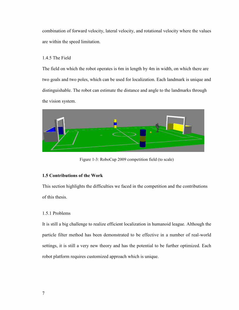
The field on which the robot operates is 6m in length by 4m in width, on which there are

two goals and two poles, which can be used for localization. Each landmark is unique and

distinguishable. The robot can estimate the distance and angle to the landmarks through

the vision system.

Figure 1-3: RoboCup 2009 competition field (to scale)

1.5 Contributions of the Work

This section highlights the difficulties we faced in the competition and the contributions

of this thesis.

1.5.1 Problems

It is still a big challenge to realize efficient localization in humanoid league. Although the

particle filter method has been demonstrated to be effective in a number of real-world

settings, it is still a very new theory and has the potential to be further optimized. Each

robot platform requires customized approach which is unique.

8

Due to the nature of bipedal walking, there are significant errors in odometry as the robot

moves in an environment. The vibration introduces considerable noise to the vision

system. Furthermore, noise is added due to frequent collisions with other robots. The

variations in the vision data make the localization less accurate. Last but not least, the

algorithm must be run in real-time.

1.5.2 Contributions

The primary contribution of this work is the development of a switching particle filter

algorithm for localization. This algorithm improves the accuracy and is less

computational intensive compared to the traditional methods. A particle reset algorithm is

first developed to aid in the switching particle filter. The simulation results show that the

algorithm can work effectively. The algorithm will be discussed in detail in Chapter 4.

Another contribution is customizing the particle filter based localization algorithm to our

robot platform. Due to the limited process power of the PC104, a lot of effort is put in to

reduce the processing time and to increase the accuracy of the result. We explored many

ways to build the motion model and the vision model. A relatively better way to build the

motion model is to use robot kinematics. Moreover, the error for the motion model is also

studied.

For the vision model, despite the significant distortion of the fisheye lens image, we

developed a very simple vision model through the projection model of the fisheye lens to

9

extract the information from the image. Finally, all of these algorithms for localization

are integrated in our robot program and tested on our robot.

1.6 Thesis Outline

The following thesis’s chapters are arranged as follows:

In Chapter 2, we introduce the related work and the background of the robot localization

and particle filters. In Chapter 3, the architecture of the software system and the

localization module are presented. We also present how to build the motion model and

the vision model of the robot. In Chapter 4, the simulation result of the new particle reset

algorithm and the new switching particle filter algorithm are shown. In Chapter 5, how

we implement the algorithm on RO-PE VI is presented. Finally we will conclude in

Chapter 6.

10

CHAPTER II

LITERATURE REVIEW

In this chapter, we examine the relevant background for our work. First, an overview on

localization is presented. In the second part, relevant work on particle filter is discussed.

The works related to motion model, vision model and resampling skill are examined.

2.1 Localization

The localization problem has been investigated since the 1990s. The objective is to find

out where the robot itself is. The localization problem is the most fundamental problem to

providing a mobile robot with autonomous capabilities [9]. Borenstein [10] summarized

several localization techniques for mobile robot using sensors. In the early stages, the

Kalman filters are widely used for the localization but later on, particle filtering is

preferred due to the robustness. Guttman and Fox [11] compared grid-based Markov

Localization, scanning matching localization based on Kalman Filter and particle filter

Localization. The result shows that the particle filter localization is more robust. Thrun

and Fox [2, 12] showed the advantages of the particle filter algorithm and described the

algorithm in detail for mobile robot. Currently, the particle filters are dominant in robot

self-localization.

11

David Filliat [13] classifies the localization strategies into three categories depending on

the cues and hypothesis. These categories coincide with Thrun’s classifications which we

referred in Chapter 1. Many researchers explored the localization problem for mobile

robot with different platforms and in different environment. Range Finder is employed as

the distance detector on many robots. Thrun [1] mainly addressed the range finder to

show the underlying principle for the mobile robot localization. Rekleitis [14] also use

the range finder to realize the localization.

2.2 Localization in RoboCup

Early time in RoboCup, the mobile robot uses the range finders to help in the self-

localization. Schulenburg [15] proposed the robot self-localization using omni-vision

and laser sensor for the Mid-size League mobile robot. Some time later, it is not allowed

to use range finders in RoboCup field, because the organizer wants to improve the human

characteristic of the robots. Marques [16] provided a localization method only based on

omni-vision system. But this kind of camera is also banned several years later. Only

human-like sensors can be employed. In the end, Enderle [17, 18] implemented the

algorithm developed by Fox [19] in the RoboCup environment.

After the mobile robot localization is introduced into RoboCup, the researchers started to

explore the localization algorithm for legged robots. Lenser [20] described a localization

algorithm called Sensor Resetting Localization. This is an extension of Monte Carlo

Localization which significantly reduced the number of particles. They implemented the

algorithm successfully on Sony Aibo, which is an autonomous legged robots used in

12

RoboCup’s Standard Platform League. Röfer [4, 21, 22] contributed to improve the

localization for legged robot self-localization in RoboCup. He proposed several

algorithms to make the computation more efficient and using more landmarks to improve

the accuracy of the result. Sridharan [23] deployed the Röfer’s algorithm on their Aibo

dogs and provided several novel practical enhancements. Some easy tasks are also

performed based on the localization algorithm. Göhring [24] presented a novel approach

using multiple robots to cooperate by sharing information, to estimate the position of the

objects and to achieve a better self localization. Stronger [25] proposed a new approach

that the vision and localization processes are intertwined. This method can improve the

localization accuracy. However, there is no mechanism to guarantee the robustness of the

result. This algorithm is quite sensitive to large unmodeled movements.

Recently, the literature on localization is mainly on humanoid robots. Laue [26] shifted

his four legged robot localization algorithm onto biped robot. The particle filter is

employed for self-localization and ball tracking. Friedmann [27] designed the software

framework. They use a landmark template (used for short memory) to remember the

landmarks, and use the Kalman-filter to pre-process the vision information, followed by

the use of particle filter to realize the self-localization. Strasdat [28] presented an

approach to realize a more accurate localization, which involves applying Hough

transform to extract the line information, which yields a better result than only using the

landmark information.

13

Localization algorithm had been developed for RO-PE series before. Ng [6] developed

the robot self localization algorithm based on triangulation, it is a static localization

method. The drawback is that the robot must remain still and pan its neck servo to get the

landmark information of the surroundings. Because of the distortion of the lens, only the

center region information of the lens is utilized. This method is quite accurate if there is

no interference but not practical because of the highly dynamic environment in RoboCup

competition.

2.3 Particle Filter

The particle filter is an alternative nonparametric implementation of the Bayes filter. Fox

and Thrun [2] developed the algorithm for mobile robot to estimate the robot’s pose

relative to a map of the environment. The following researchers worked on the

improvement of the motion model, vision model and the resampling method of the

particle filter.

2.3.1 Motion Model

The motion model is used to estimate relative measurements, which is also referred to as

the dead reckoning. Abundant research is done for the motion model of the wheeled

mobile robots. The most popular method is to acquire the measurements by odometry or

inertial navigation system. Rekleitis [14] described how to model the rotation and the

translation of the mobile robot in detail. The motion model includes the odometry and the

noise. Thrun [1] proposed an approach to realize the odometry by a velocity motion

14

model, which is more similar to the original odometry used on ship and airplane. This

approach is comprehensive because the mobile robot performs a continuous motion.

Inertial navigation techniques use rate gyros and accelerometers to measure the rate of

rotation and acceleration of the robot, respectively. A recent detailed introduction to

inertial navigation system is published by Computer Laboratory in Cambridge University

[29]. There is also some inspiring research on measuring the human position using the

inertial navigation system. Cho [30] measures the pedestrian walking distance using a

low cost accelerometer. The problem is that only the distance is measured without

orientation, and the accelerometer is only used for counting the steps.

However, the motion model of the humanoid robot is still not well studied. Many

researchers consider that the motion model for legged robots is very complex, especially

for bipedal robots. For humanoid robot, what we are controlling is the foot placement. If

we can know exactly where the next planned step is, we can directly get the displacement

information from the joint trajectories instead of integrating the velocity or acceleration

of the body.

2.3.2 Vision Model

The RoboCup Humanoid Robot, according to the rules, can only use human-like sensors.

The most important sensor is the camera mounted on the head of the robot, which can get

the projective geometry information of the environment. Jüngel [31] presented on the

coordinate transformations and projection from 3D space to 2D image for a Sony Aibo

15

dog. Ng [6] developed the vision system and the algorithm for image segmentation and

object classification for RO-PE VI (Fig 2-1). He described the implementation of

OpenCV (Intel Open Source Computer Vision Library), and proposed the method to

realize the cross recognition and line detection.

Röfer [21, 22] did a lot of work in the object classification for localization and how to use

the data extracted from the image. All the beacons, goals and direct lines are extracted

and used for localization.

(a) (b)

(c)

Fig 2-1: RO-PE VI vision system using OpenCV with a normal wide angle lens. (a) Original

image captured from webcam. (b) Image after colour segmentation. (c) Robot vision supervisory

window. The result of object detection can be labelled and displayed in real time to better

comprehend what the robot sees during its course of motion.

16

In Fig 2-1, the preliminary image and the processed imaged obtained by the RO-PE VI

vision system are shown. The fisheye lens has super wide angle and the distortion is

considerable. Because of the limited computational power of the industry PC104 and the

serious distortion, the final program executed in RoboCup 2008 did not include the cross

recognition and line detection functions. Therefore, during the actual competition, our

robots can only recognize the goals and poles, which are all color labeled objects.

2.3.3 Resampling

The beauty of the particle filter is resampling. Resampling is to estimate the sampling

distribution by drawing randomly with replacement from the original sample. Thrun [1]

presented a very comprehensive description of the importance of resampling and

discussed some issues related to the resampling. They discussed the resampling method

when the variances of the particles are rather small. Rekleitis [32] described three

resampling methods and provided the pseudo code for the algorithm. The simplest

method is called select with replacement. The algorithm for this method is presented in

chapter 3. Linear time resampling and Liu’s resampling are also discussed in Rekleitis’

paper.

17

CHAPTER III

PARTICLE FILTER LOCALIZATION

In the previous chapters, we introduced the localization problem, the particle filter

method and many literatures on it. In this chapter, we are going to present the algorithm

for the localization on our robot. We will focus on the motion model, vision model and

the resampling in the particle filter localization algorithm.

3.1 Software Architecture of RO-PE VI System

We will give an overview of the RO-PE VI software system. There are three parts of the

program running at the same time on the main processor (PC104). The vision program

deals with the image processing, and passes the perceived information to the strategy

program through the shared memory. Strategy program makes decisions based on the

vision data and sends the action commands to motion program. In the end, the motion

program executes the commands by sending information to the servo. Fig 3-1 shows the

main flow of the program.

Our localization program is based on passive localization approach. In this approach, our

localization module reads the motion command of the robot from the strategy and obtains

the data from vision program to perform localization. The robot will not perform a

18

motion just to localize itself. The localization program is independent of the decision

making program as it processes only the motion and vision data and does not directly

modify the decision making algorithm.

Fig 3-1: Flowchart of RO-PE VI program and the localization part

3.2 The Kinematic Configuration for Localization

We need to build a global coordinate system and the ego-centric coordinate of the robot

to describe the localization problem. The robot pose contains robot position in the 2D

plane and heading. The coordinate system and one robot pose are shown in Fig 3-2:

The ego-centric coordinate of the robot is Rxryr. The particles within the particle filter

algorithm represent pose values ( ), ,x y θ which are expressed in the global coordinate

system Oxoyo (Fig 3-2). θ is used to indicate the robot heading (xr) with respect to xo axis.

19

0x

0y

( )x y,

θrx

ry

Fig 3-2: The layout of the field and the coordinate system, the description of the particles

3.3 Particle Filter Algorithm

We have briefly introduced the particle filter in Chapter 1. The detailed algorithm is

presented in this section. The general particle filter algorithm is presented in Fig 3-3

(Adapted from [1]). What we called particles are samples of the posterior distribution Xt,

which is also called the pose or state of the robot. In this particular localization problem,

each particle xt contains the position and heading of the robot. The number of the

particles is M. Therefore, the set of particles are denoted

[1] [2] [ ]: , , M

t t t tX x x x= K (3-1)

The input for the particle filter algorithm is the set of particles Xt-1, the recent motion

control command ut and the recent perceived vision data set zt. The algorithm processes

the input sample set t -1X in two passes to generate an up-to-date sample set tX . During

the first pass, each particle t -1x is updated according to the executed motion command tu

(based on the motion model which will be described later) at the fourth line of the

20

algorithm. After that, the weight tw of the particle is computed based on the perceived

data set tz (which is the vision model which will be described later) at the fifth line of

the algorithm. We form a new temporary set tX and each state contains the updated tx

and the importance weight tw . The importance weights actually incorporate the

perceived data tz into the updated state.

Fig 3-3: Particle Filter Algorithm [1]

In the second pass, the new set tX is created by randomly drawing elements from tX

with probability which is proportional to their weights. This pass is called resampling

(line 8 to 11). Resampling transforms a set of M particles into another particle set of the

same size. By incorporating the importance weights into the resampling process, the

distribution of the particles changes. Before the resampling step, they were distributed

according to the belief ( )avg tbel x , after the resampling they are distributed

1: Algorithm Particle_filter( 1, ,t t tX u z− ):

2: t tX X φ= =

3: for 1m = to M do

4: sample ( )[ ]

1,m m

t t t tx p x u x −:

5: ( )[ ] [ ]m m

t tw p z x=

6: [ ] [ ],m m

t t t tX X x w= +

7: end for

8: for 1m = to M do

9: draw i with probability [ ]i

tw∝

10: add [ ]i

tx to tX

11: end for

12: return tX

21

(approximately) according to the posterior ( ) ( ) ( )[ ]m

t t t avg tbel x p z x bel xη= . In fact, the

resulting sample set usually possesses many duplicates, since particles are drawn with

replacement.

In the whole algorithm, the content of each particle, the motion model and sensor model

(vision model) need to be built based on different particular system. They may vary from

one system to another. But the resampling algorithm is the unchanged part in the particle

filter algorithm (though it can be optimized sometimes according to different system).

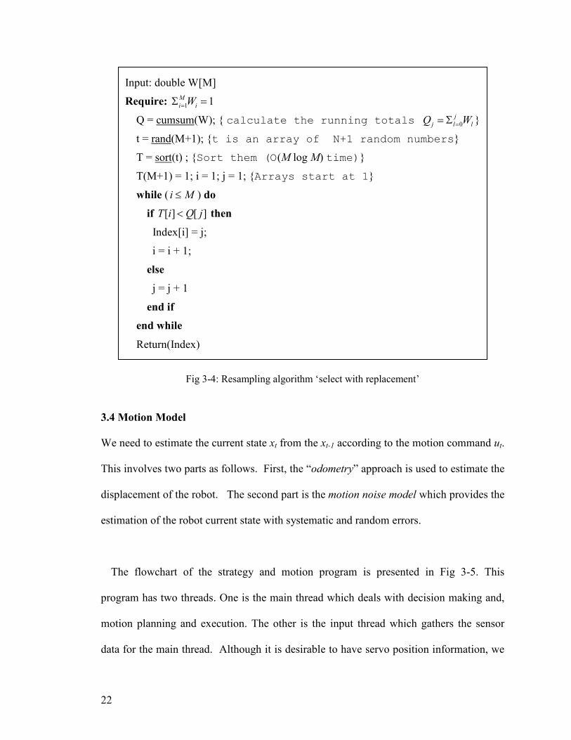
We present the detailed resampling algorithm - ‘select with replacement’ - [32] in this

subsection.

The simplest method of resampling is to select each particle with a probability equal to its

weight. In order to do that efficiently, first the cumulative sum of the particle weights are

calculated, and then M sorted random numbers uniformly distributed in [0,1] are selected.

Finally, the number of the sorted random numbers that appear in each interval of the

cumulative sum represents the number of copies of this particular particle which are

going to be propagated forward to the next stage. Intuitively, if a particle has a small

weight, the equivalent cumulative sum interval is small and therefore, there is only a

small chance that any of the random numbers would appear in it. In contrast, if the weight

is large, then many random numbers are going to be found in it and thus, many duplicates

of that particle are going to survive. The detailed procedure is presented in Fig 3-4.

22

Fig 3-4: Resampling algorithm ‘select with replacement’

3.4 Motion Model

We need to estimate the current state xt from the xt-1 according to the motion command ut.

This involves two parts as follows. First, the “odometry” approach is used to estimate the

displacement of the robot. The second part is the motion noise model which provides the

estimation of the robot current state with systematic and random errors.

The flowchart of the strategy and motion program is presented in Fig 3-5. This

program has two threads. One is the main thread which deals with decision making and,

motion planning and execution. The other is the input thread which gathers the sensor

data for the main thread. Although it is desirable to have servo position information, we

Input: double W[M]

Require: 1 1M

i iW=Σ =

Q = cumsum(W); { calculate the running totals 0

j

j l lQ W== Σ }

t = rand(M+1); {t is an array of N+1 random numbers}

T = sort(t) ; {Sort them (O(M log M) time)}

T(M+1) = 1; i = 1; j = 1; {Arrays start at 1}

while ( i M≤ ) do

if [ ] [ ]T i Q j< then

Index[i] = j;

i = i + 1;

else

j = j + 1

end if

end while

Return(Index)

23

are currently unable to obtain the servo position information from the hardware. The

servo position feedback is shown as a dashed block in Figure 3-5 to indicate future

implementation. In the current stage, the servo position command is considered to be ut.

Fig 3-5: Flowchart of the motion and strategy program

3.4.1 Kinematic Motion Model

The robot kinematics used for calculating the translation and rotation of the robot is

presented in this subsection.

24

The motion model for humanoid robot has seldom been discussed in the literature. In this

research, we proposed an algorithm which uses motion command to identify every step

and calculate the accumulated displacement of the robot, for both the translation and the

rotation of the robot. This algorithm is inspired by the pedestrian odometry, a step

counter uses average step length to estimate the accumulated distance travelled by a

person.

The actual motion information of the robot is estimated from the servo commands which

are sent to the servos. A forward kinematic model is then used to calculate the hip and

ankle position in the Cartesian space. Based on the kinematics analysis included in

Appendix A, we can obtain the incremental updates to the state variables (∆x, ∆y, ∆θ) for

each step.

3.4.2 Noise Motion Model

From the motion model, we can get ( ), ,x y θ∆ ∆ ∆ . The noise motion model provides

uncertainties in the real world, due to the imprecise model of the robot and the

environment imperfections. In the past, not enough attention has been paid to the motion

model error. A simple Gaussian noise was simply added to the final position of the robot.

Rekleitis [32] proposed a detailed precise odometry error model for the mobile robot.

Thrun [1] tuned some parameters in the noise motion model, and added in different noise.

For the mobile robot, the difficulty is that the rotation noise will affect the final position

of the robot, which is hard to model, because the motion error is random. For humanoid

25

robot, we can simply add noise to the final position of one step since we only update the

odometry during the double support phase. Regardless how the legs swing, we can get the

final configuration from the servo position information once the swing foot touches the

ground.

[ ] [ ]

1 ()m m

t t x xx x x S R random−= + ∆ + + × (3-2)

[ ] [ ]

1 ()m m

t t y yy y y S R random−= + ∆ + + × (3-3)

[ ] [ ]

1 ()m m

t t S R randomθ θθ θ θ−= + ∆ + + × (3-4)

[ ]m

tx , [ ]

1

m

tx − and x∆ represent current state, previous state and the incremental state update

respectively. Sx, Sy and Sθ are the systematic error; Rx, Ry and Rθ are the maximum

random error; random() is a function generating random number within [-1, 1]. We add

the errors to the displacement and the orientation to provide uncertainty modeling for the

actual pose change detection. Every other step we will update all the particles according

to the pose change.

3.5 Vision Model

In this section, we will describe the vision model developed for RO-PE VI robot in detail.

The vision model is used in the update stage of the particle filter algorithm, in particular,

the fifth line in Fig 3-3.

3.5.1 The Projection Model of Fisheye Lens

The projection model of the camera and the camera calibration are important because it

can relate the image data with the real, three-dimensional world data. Hence, the mapping

26

between the coordinates in the image plane and the coordinates in the physical 3D space

is a critical component to reconstruct the real world.

The mathematical model of the central perspective projection (This is also known as

pinhole camera model) is based on the assumption the angle of incidence of the ray from

an object point is equal to the angle between the ray and the optical axis within the image

space. The light-path diagram is shown in Fig 3-6(a).

The fisheye projection [33] is based on the principle that in the ideal case the distance

between an image point and the principle point (image center) is linearly dependent on

the angle of incidence of the ray from the corresponding object point. The light-path

diagram for fisheye lens is shown in Fig 3-6(b).

(a) (b)

Figure 3-6: (a) Central perspective projection model, we have 1 1α β= and 2 2α β= . (b) Fisheye

projection model, we have 1 2

1 2d d

α α=

27

3.5.2 Robot Perception

After establishing the model of the fisheye lens, we need to get the differences between

the perceived data and the estimated data to update the particles’ weights. We update the

weight of each particle according to the angle and the distance difference respectively.

3.5.2.1 Angle

Due to the projection principle [34], we need to choose certain points of the landmarks.

We can always find out the representation of these points in the image plane. In our

calculations, as shown in Fig 3-7, we use the center of the pole (point A in Fig 3-7 a) and

the 2 sides of the goal (points B and C in Fig 3-7 b). In the image plane, the mid-point of

the pole can represent the center of the pole in Cartesian space. Similarly, the two edges

of the goal in the image can represent the two goalposts. Fig 3-7 indicates the projective

relationship between the chosen points and corresponding points in the image. The dash

lines in Fig 3-7 are the angle bisector.

x

y

Pole

Robot

Robot

A

(a) (b)

Fig 3-7: The projective model of the landmarks. (a)The view of the pole projected to the image.

(b)The view of the goal projected to the image

28

According to the fisheye lens optical model it is not difficult to get the angle perceivedθ

from the landmark to the orientation of robot’s head. The predicted angle expθ can be

calculated from the predicted particle position, the neck servo position and hip yaw servo

position. Based on these data, we can get the angle from the landmark to the orientation

of the robot (the detailed derivation of perceivedθ is included in Appendix B). The predicted

angle expθ can be calculated by geometry. We can obtain the angle difference ∆θv:

v exp perceivedθ θ θ∆ = − (3-5)

3.5.2.2 Distance

Only knowing the angles of the landmark respect to the robot is not enough. There are

more information can be used from the image. We need to include the distance

information into the localization algorithm.

The distance from the landmark to the robot can be estimated through the size of the

landmark on the image. Because the focal length of the lens is only 1.55mm, so we can

consider that all the landmarks are far away that the image is on the focal plane.

According to the fisheye lens model described previous, we can discover that the size of

the landmark on the image is always the same if the distance from the landmark to the

robot is constant, regardless with the angle perceivedθ . This characteristic of the fisheye lens

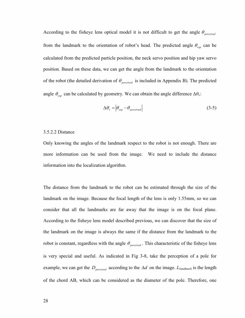
is very special and useful. As indicated in Fig 3-8, take the perception of a pole for

example, we can get the perceivedD according to the d∆ on the image. Llandmark is the length

of the chord AB, which can be considered as the diameter of the pole. Therefore, one

29

determined perceivedD has certain corresponding α∆ and d∆ . We can use the height of the

goal and the width of the pole to determine the distance from the landmark to the robot.

(For the detailed derivation please see Appendix B) The theoretical explanation in this

section is quite abstract. We will implement all these results in Chapter 5, to build the real

vision model for the robot. It will be more practical and intuitive.

L landmark

Fig 3-8: Derivation of the distance from the robot to the landmark

We can get expD from the predicted particle position and the landmark position. When

calculating the angle difference, we are using the absolute difference of the angle as the

error. But we cannot use the absolute difference for the distance information, because

when expD is large, the error will be large also. We use the absolute error over the smaller

distance as the distance difference. In Equ(3-6), if we change the value of Dexp and

Dperceived, we can get the same result. The relative distance difference ∆D:

min( , )

exp perceived

exp perceived

D DD

D D

−∆ = (3-6)

30

3.5.3 Update

Now we have both the ∆θv and the ∆D for a certain landmark. A standard normal

distribution is employed to calculate the weight and update the weight for each particle.

2

v1

21

2

tbelief e

θθ

θ π

∆−

∆ = ,

21

21

2

t

D

D

Dbelief eπ

∆−

∆ = (3-7)

This is a normal distribution. We employ two new parameters called angle tolerance and

distance tolerance, θt and Dt. These two parameters are the errors what we can afford. If

we want most of the particles converge to a cluster in which most of their angle errors are

within π/12, we can choose θt as π/12. Dt is a ratio, we can choose it as 1, that means we

can afford that the Dperceived is within [Dexp /2, 2 Dexp].

In the end we update the weight.

v

[ ]

,

m

i

D

w beliefθ∆ ∆

= ∏ (3-8)

Pay attention that only when the landmark is perceived, we will update every particle’s

weight.

31

CHAPTER IV

SIMULATION

In the previous chapter we build the motion model and the vision model for RO-PE VI.

We need to verify whether the landmark information is enough for us to realize the

localization effectively, or if the algorithm can employ fewer particles. We developed the

simulation code in MatLab™, which is more convenient for debugging the parameters

and testing the algorithm. Most important, a novel and intuitive resetting algorithm is

presented and a new switching particle filter algorithm is developed.

4.1 The Simulation Algorithm

In this section we will give a detailed description of our simulation method. The main

part of the particle filter is the same as what we showed in chapter 3, algorithm presented

in table 3-1. We do not need to build the motion model and the vision model of the robot,

but calculate the information through the geometry relationship of the robot pose and the

coordinates of the landmarks. The motion model and vision model are only several lines

code in MatLab™. We add on different noise to the input data to simulate the error from

motion model and vision model, intend to test the robustness of the particle filter

algorithm.

32

In general, the particle filter algorithm needs around over one thousand particles to get

the accurate result. However, our system cannot afford the expensive computation. But if

we use too few particles, the accuracy of our localization will not meet our requirement.

There is a question: How many particles do we need for the localization in RoboCup

scenario? We use different number of particles to test the algorithm and compare the

result. We also add in a teleport in the simulation to test the robustness of the algorithm.

4.1.1 Particle Reset Algorithm

Thrun and Lenser [1, 20] present the algorithm of resetting the particle filter respectively.

The purpose of resetting the particle filter is to increase the variance of the particles. This

is very useful when the number of particles is small. Here we will propose a simple but

effective resetting method.

In practice, when the particles converged, they are difficult to get out of the current

position to search for a better place, since the state space is too large to be covered

appropriately. This problem is even worse when the robot does not know the initial

position or it is teleported to some where else. One solution is to discard some particles

with low probability and randomly throw them into the field again. We call these

particles need to be reset bad particles. But we need to find a certain way to select these

particles. In our algorithm, we have the angle information and distance information. The

belief is based on all the landmarks we perceived and the differences we calculated from

the observation and the estimation. Due to the different number of the landmarks we can

see every time when updating the weight of the particles, it is difficult to set a threshold

of the weight to decide whether we need to reset some particles. Our method is to reset

33

the particles those are totally impossible. If there is one of the landmarks seems in the

correct place respect to any landmark information, we will not reset this particle. That

means only if all the perceived landmarks are obviously different from the estimated

ones, we will reset this bad particle. The advantage of this algorithm is that even though

the vision program mistaken one of the landmarks, or there is some interference in the

circumstance, most of the particles will still stay in the right place. If there is really some

teleport happened, almost all of the particles will have the chance to be thrown into the

field again and they can converge to a new place again. With this particle reset algorithm,

the particle filter based localization algorithm can easily handle the kidnapped robot

problem.

It is important to understand this particle reset algorithm. It is not difficult to count the

number of reset particles. And the new developed switching particle filter algorithm

presented in the next section is based on counting the bad particles.

4.1.2 The Switching Algorithm of the Particle Filter

This algorithm is a kind of adaptive particle filter algorithm. Generally, the localization

of a kidnapped robot problem can be divided into the global localization and the local

position tracking. These two procedures are alternating to handle the teleportation and the

incremental movement respectively. The conventional particle filter does not have an

obvious switch between the global and the local procedures, but using the particle reset

algorithm or other correction method to increase the variety of the particles and drive the

particles toward the right position. In our particle filter localization, we separate these

34

two parts and employ different number of particles for the two parts. As stated previously,

we can count the number of the bad particles easily. We switch the algorithm between

the two statuses according to the percentage of the bad particles. The detailed algorithm

is shown in Fig 4-1.

Fig4-1: The switching particle filter algorithm

35

The conventional particle filter algorithm is within the dashed box. The pose calculation

will be discussed in the next section and this procedure will not change the essence of the

particle filter but only provide an output. The key points in this algorithm are the switches

between the global localization and the local tracking. Mg is the number of particles that

the algorithm begins with. In the first several cycles, there will not be enough particles

meet the requirement and the bad particles are still more than 10%, the two switches will

not be activated and the whole algorithm is the same as the conventional one. When the

particles are converged enough and the bad particles are less than 10%, we randomly

draw Ml particles from the current data set and start a new cycle (The Mg are much

greater than Ml). When the robot is teleported or intense collision happened to the robot,

the bad particles are suddenly increased and more than 90%, we will restart the whole

algorithm. The result of this switching algorithm can reach the particle filter with Mg

particles but running time is almost the same as the particle filter with Ml particles.

4.1.3 Calculation of the Robot Pose

After running the particle filter algorithm, we will have a converged cluster of particles.

But what we need is an exact output, the robot pose information. We need to abstract a

final estimation representing the pose of the robot from the set of particles. Laue [35]

proposed several ways to calculate the robot pose from a given set of particles: overall

averaging, best particle, binning, k-means clustering and particle history. We choose the

simplest and most efficient one: take the particle with highest weight as the output of the

algorithm.

36

4.2 Simulation Result of the Conventional Particle Filter with Particle Reset

Algorithm

In this section we will test the conventional particle filter with our particle reset algorithm

in MatLab™ (The detailed MatLab™ code is presented in Appendix C). The kinematic

configuration in this chapter is the same as we described in Chapter 3, Fig 3-2. The unit

for x and y is meter and for θ is radian. We will do comparison on the running time and

accuracy when employ different number of particles.

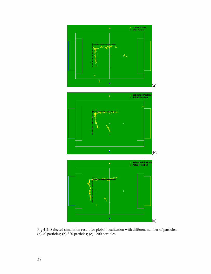
4.2.1 Global Localization

Firstly we show a result of the particle filter when doing the Global Localization. The

black particles are the real robot position and the yellow ones are the estimated positions.

As shown in Fig 4-2, the robot start from the position (1.5, 1.5, Pi/2), go straight to (1.5,

3.5, Pi/2), turn to (1.5, 3.5, 0), then go straight to (3.5, 3.5, 0). In the simulation, the step

we are using is 0.05m; the angle interval is Pi/10 when turning. The threshold for particle

reset is 0.3 for distance and Pi/8 for the angle. The maximum random error Rx, Ry and Rθ

are 0.1, 0.05 and Pi/6 respectively. In the simulation we did not consider the systematic

error. The threshold for particle reset and the noises are all the same for the following

simulations.

In the simulation result we show the actual trajectory and the estimated trajectory formed

by the actual positions and estimated positions every cycle. We can see from Fig 4-2,

although some particles are quite far from the real route, most of the estimated positions

are within a certain range of the actual position. After running the program with different

37

(a)

(b)

(c)

Fig 4-2: Selected simulation result for global localization with different number of particles:

(a) 40 particles; (b) 320 particles; (c) 1200 particles.

38

number of particles many times, for the global localization we can observe that: the more

the particles are, more stable and more accurate the localization result is. Sometimes

when using 40 particles, it will also appear perfect result. But take an average, the result

of particle filter with 1200 particles are much better than the particle filter with 40

particles. The results shown in this thesis are selected results. Though the results are not

shown exact error and converging cycles, they are still representative.

The time to finish the simulation for 40 particles, 320 particles and 1200 particles are 6s,

21s and 88s respectively. In the simulation, it is quite obvious that when we using more

particles, it is easier for the particles to converge and closer to the actual position. If we

are using 40 particles, it is take almost 30 to 40 cycles to reach to a satisfied place.

4.2.2 Position Tracking

What we called position tracking is that we know the initial pose of the robot. According

to the rules of the RoboCup Humanoid League, most of the time we will always know the

starting position and orientation of the robot. So this time we will manually set several

particles at the three starting places instead of randomly distribute all the particles.

The simulation results are shown in Fig 4-3. In the simulation, we set two particles at

each three initial positions. The robot is starting from one of them: (1.5, 3.5, 0), then turn

to (1.5, 3.5, -Pi/4), go straight to around (2.9, 3.1, -Pi/4), then go straight to the center of

the field and hugging back. This path is imitating the real condition during the

competition. The starting position is the position where we put the robot when the game

begins. Actually there are only 10 positions where the robot can be put when starting,

39

(a)

(b)

(c)

Fig 4-3: Selected simulation result for position tracking with different number of particles.

(a) 40 particles. (b) 320 particles. (c) 1200 particles

40

exclude the goalkeeper position. So it is totally possible that at the first beginning we set

part of the particles at these 10 positions, it will improve the convergence of the particles.

From the simulation result we can observe that if we know the initial pose of the robot, it

is enough to track the position and orientation with only 40 particles. The time to finish

the simulation for 40 particles, 320 particles and 1200 particles are 5s, 22s and 90s

respectively. Because in the simulation we manage to run same number of cycles, the

time consuming is also quite similar to the global localization problem.

4.2.3 Kidnapped Problem

It seems that 40 particles are enough for localization in RoboCup Humanoid League

scenario since we can always estimate the initial positions of the robot. However, we still

need to improve the algorithm because of intense collision and most important: the

limitation of our RO-PE VI vision system and the noisy motion model.

In our system, the camera is chosen by the strategy part, which is the decision making

part of the program. Because of the complexity of the strategy, we only do passive

localization. In the real condition, it is not using the wide angle camera all the time, but

also need to use the pin-hole camera which can see much further. Because the pin-hole

camera has a very small angle view, we did not develop the landmark recognition for the

pin-hole camera. The problem comes. If the robot use the pin-hole camera perceives the

ball which is quite far away, it will track the ball and until move to the ball within a

certain distance, then change to wide-angle lens camera. That means, the robot will have

some time cannot perceive any landmarks, but only walk blindly, and it can only estimate

41

its pose based on the odometry. And this time, we do not know exactly where the robot

is. With our particle reset system, the localization is become another global localization.

Our simulation result for the global localization shows that 40 particles are not enough

for the fast convergence and high accuracy.

Fig 4-4: The simulation result for odometry result without resampling

We will show the simulated odometry result for the robot in Fig 4-4. We show the

odometry result every 20 steps. It is obvious that after 80 steps, the estimated position is

already far from the actual position. In real condition, the result may be worse due to

some undetected fierce collision.

From the image at least we know that if the robot walk blindly for some time, the error

will be very large. So we can consider it as a kidnapped problem. We make the robot in

an extreme condition and test the robustness of the localization system. The robot starts

from the position (1.5, 1.5, Pi/2), go straight to (1.5, 3.5, Pi/2), turn to (1.5, 3.5, 0). Then

we teleport the robot to (4.5, 2.5, -Pi). If the algorithm can recover from this situation, it

42

(a)

(b)

(c)

Fig 4-5: Selected simulation result for kidnapped localization with different number of particles:

(a) 40 particles; (b) 320 particles ; (c) 1200 particles.

43

definitely shows that the algorithm is robust enough to handle the kidnapped localization

problem in RoboCup scenario. The simulation results are shown in Fig 4-5. It is obvious

that more particles, better the recovery from teleporting. The time to finish the simulation

for 40 particles, 320 particles and 1200 particles are 9s, 27s and 108s respectively.

4.3 The simulation of the switching particle filter algorithm

From the simulation result we can observe that there is a trade off between the accuracy

and the computational time for the kidnapped problem. How to achieve the accuracy and

save the computational time is our main objective.

We developed the switching particle filter algorithm. It takes advantage of the better

initial convergence for more particles and computational efficiency for fewer particles

when do the position tracking. The main part of the switching algorithm is discussed in

section 4.1.2 and we will show the technical detail and the simulation result in this

section.

When initialize, we distribute the particles every 0.6m in x direction and every 0.5m in y

direction. For each crossing, we have eight orientations from 0 to 2π with the interval π/4.

Altogether we have 648 particles at the beginning shown as in Fig 4-6(a). Theoretically,

the initial error should be less then (0.3, 0.25, π/8).

We can count the number of particles which will be reset every cycle. At beginning, there

will be definitely more than 10% particles need to be reset. We consider there are too

many bad particles, and the result is not reliable, so the final estimation is painted in blue.

44

If the number of reset particles is less than 10%, we consider the convergence is already

done and the result can meet the requirement, we show the result in yellow. And this is

the time to switch to tracking mode. During tracking mode, we always consider the result

can meet the requirement. Now we randomly select 40 particles from the 648 particles to

do the position tracking. When we teleport the robot to a new place, we still count the

number of reset particles. If the reset particles are more than 90%, we consider we need

to do the global localization again, so we switch back to the initialization of localization

and mark the result unreliable again.

(a)

(b)

Fig 4-6: Grid-based localization with position tracking. (a) The initial positions of the distributed

particles. (b) Selected result of the algorithm.

45

The time to finish this simulation is 8s. We can see from Fig 4-6(b) that the result is more

accurate than when we are using the conventional particle filter with 40 particles, but the

time is almost the same.

4.4 Conclusion

We aim to achieve high accurate and efficient localization. After testing the global

localization, position tracking and the kidnapped problem, we find out the characteristic

of the particle filter localization and developed a new Grid-based with position tracking

localization, and use the proposed particle reset algorithm as the criteria to do the whole

resetting. Finally, we can realize the localization very accurately and fast. Next, we need

to implement the algorithm on our robot and consider the noise brought in by the sensors.

46

CHAPTER V

IMPLEMENTATIONS

In this chapter, we need to build the proposed motion model and vision model in chapter

3. We will present how to get the practical vision model and motion model, (for the

theoretical background the reader need to refer to the Appendix A and B) and then

discuss some issues when transplant the localization algorithm to the robot PC104

system. In the end, we will show the experiment result and conclude.

5.1 Introduction

Firstly, we will give a brief introduction to the robot soccer strategy. And what we refer

to as strategy is the decision making part mentioned in Fig 3-1 and Fig 3-5.

Fig 5-1: Brief flowchart of the robot soccer strategy

This is a simplified flowchart for the robot soccer behavior. After starting up, the robot

will look for the ball. When seeing the ball, it will try to walk to the ball. The robot needs

to align itself to the goal when reaches the ball. The final stage is kicking the ball to the

goal. There is no complicated strategy such as dribbling or passing. Whenever the robot

47

lose track of the ball, it will search for the ball again. When the robot is moving, the

localization algorithm is called every other step during the double support phase. The

localization algorithm is also called after the robot standing still and panning its neck

servo to search for ball, during the look for ball stage. We create a short-term memory to

remember the landmark perceived during the scanning. As mentioned in Chapter 4, when

the robot walk to a ball which is far away (further then 1.2m), the pinhole camera is

employed. In this period, though the localization function is called, there is no landmark

information updated, so the output equals the odometry reading with noise added.

The drawback of the current strategy is that if the robot cannot actively walk around the

field to search for the ball, what the robot can only do is looking around until the ball

comes to its view. With the localization information, the robot can move to other part of

the field to search for the ball. And if the ball is within possession of one robot, the other

robots can move to a place where can take advantage of. In the current stage, we can

obtain enough information to perform the localization with the current strategy. And we

do not change the strategy architecture to improve the localization result or perform some

other complicated tasks. Firstly, it is necessary to come out an applicable localization

result.

5.2 Experiments for motion model and vision model

In chapter 3 we present how to build the motion model and the vision model. And we

also mentioned that we need to obtain some data from the experiments. In this section we

will carry out experiments to determine the parameters for motion model and vision

48

model. These experiments are also good supplement for the theoretical part described in

chapter 3.

5.2.1 Experiment for Motion Model

The parameters we need to obtain for the motion model are systematic error Sx, Sy, Sθ and

random error Rx, Ry and Rθ mentioned in Equation(3-2,3-3,3-4). We take the experiment

to obtain Sx and Rx as example to show the procedure.

Fig 5-2: The odometry value and the actual x displacement measurement

We did experiment on the error of the odometry model. The odometry result and the real

measurement are shown in Fig 5-2. The maximum error for one step occurs at the first

step and the minimum error occurs at the second step. We simply take the minimum error

as Sx and the difference between the maximum error and the minimum error as Rx. The

selection of parameters can make the result of noise motion model cover and surround the

actual positions of the robot when there is no collision. Though we can adopt some

advanced methods (e.g. least square means) to compute the parameters, it does not help

much for the particle filter algorithm.

49

5.2.2 Experiment for Vision Model

It is necessary to verify the vision model through experiments. Based on that, we can

obtain θperceived and Dperceived mentioned in chapter 3. In Fig 5-3, the images are captured

by the robot fish-eye lens camera when the robot is standing still. The landmark we used

for reference is the blue-yellow-blue pole. The pole is labeled by a bounding box and has

letters ‘BYB’ at the bottom.

(a) (b)

(c) (d)

Fig 5-3: Part of the images collected for the experiment: (a) The pole is put 1m away in front of

the robot. (b) The pole is put 2m away in front of the robot. (c)The pole is put 45° and 1m away

from the robot. (d)The pole is put 45° and 2m away from the robot.

We put the pole at different positions from the robot. We recorded the position of pole in

image, and also the angle and distance from the pole to the robot. According to the fish-

eye lens model presented in Fig 3-6, the position of the pole in the image should only

50

related to the angle from the pole to the robot, regardless with the distance. We will show

the experiment data in Table 5-1.

Table 5-1: Pole position in the image, according to different angles and distances

Angle 0˚ 30˚ 45˚ 60˚

Distance

1m -2 70 (2.33) 105 (2.33) 141 (2.35)

2m 0 73 (2.43) 108 (2.40) 144 (2.40)

4m -2 75 (2.50) 114 (2.53) 148 (2.47)

In Table 5-1, the first row shows the angle between the actual position of the pole and the

robot. The first column shows the distance from the pole to the robot. Because the length

of the image is 320 pixels, so we consider the pixel at the middle of the image is 0.

According to our coordinate system of the robot, the axis point to the left. We can

examine the pixel value inside the table. It is quite obvious that the pixel value is affected

by the angles significantly but rarely by the distance. We also provide the ratio (pixel

value over angle) in the bracket, which is not applicable when the angle is 0°. From Table

5-1, we verified the vision model and obtain the relationship between the landmark

positions and its position in the image. We take the average of all the ratios presented in

Table 5-1 as the coefficient and obtain the empirical equation:

2.42perceived

PixelPositionθ = (5-1)

After we obtain the perceived landmark angle θperceived, we need to work on the perceived

landmark distance Dperceived. We use the same data set as partly shown in Fig 5-3. This

time we recorded the width of the pole image, and the distance from the pole to the robot.

As shown in appendix B, we can get the distance from the landmark to the robot only

51

based on the dimension of the landmark and the number of pixels covered by the

corresponding part of the landmark in the image. The experiment data is shown in Table

5-2. The diameter of pole is 11cm, which is referred to as Llandmark in Fig 3-8.

Table 5-2 Relationship between the pole distance and the width of the pole in image

D Num of Pixels D *Pixels/Llandmark

20cm 63 114.5

50cm 27 122.7

100cm 13 118.2

200cm 7 127.3

300cm 5 136.4

In the table, D is the distance from the pole to the robot; Num of Pixels represents the

width of the pole in the image, which is counted in pixels. We can see that the value of

objective equation (D *Pixels/Llandmark) can be considered as a constant (except when the

landmark is further than 200cm, when the number of pixel is too few to give a exact

estimation). We take the average of first four values of the objective equations as the

coefficient and obtain the empirical equation:

120.7landmarkperceived

LD

PixelNum

×= (5-2)

From the experiment we can be confident of the vision model built for the robot. This

vision model is efficient and easy for calibrating. The empirical equations can be

improved if a polynomial is employed to approximate.

5.3 Localization Experiment and the Evaluation

Though we finished the particle filter algorithm in the MatLab™ and make the algorithm

more efficient, the simulation result cannot be duplicated on the robot. We need to

52

execute the complicated algorithm in a real time system. It is also a necessary to have a

module showing the localization result for evaluation.

5.3.1 Improvement on transplanting the program to an onboard PC 104

The operating system we are using is Windows 2000 with RTX, and the cycle of the

program is 25ms. In one cycle, the program cannot run as many as 648 particles, which is

number we employed in the simulation. We changed the structure of the program to fit it

into the system. The diagram is shown in Fig 5-4.

Fig 5-4: Modified structure for particle filter algorithm

With the modified structure, assume that we need to perform a particle filter algorithm

with m n× particles. We can process n particles within one cycle, and finish the whole

algorithm more than m cycles. The program can be changed into a paralleled structure

program because the prediction and update for each particle is independent. After we

calculate the weight for all the particles, the resampling is performed. The advantage of

this structure is that we can run it sequentially and control the computational cost in one

cycle. We divide the computation cost as small as the system can take, so that the system

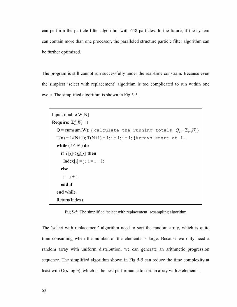
53

can perform the particle filter algorithm with 648 particles. In the future, if the system

can contain more than one processor, the paralleled structure particle filter algorithm can

be further optimized.

The program is still cannot run successfully under the real-time constrain. Because even

the simplest ‘select with replacement’ algorithm is too complicated to run within one

cycle. The simplified algorithm is shown in Fig 5-5.

Fig 5-5: The simplified ‘select with replacement’ resampling algorithm

The ‘select with replacement’ algorithm need to sort the random array, which is quite

time consuming when the number of the elements is large. Because we only need a

random array with uniform distribution, we can generate an arithmetic progression

sequence. The simplified algorithm shown in Fig 5-5 can reduce the time complexity at

least with O(n log n), which is the best performance to sort an array with n elements.

Input: double W[N]

Require: 1 1N

i iW=Σ =

Q = cumsum(W); { calculate the running totals 0

j

j l lQ W== Σ }

T(n) = 1/(N+1); T(N+1) = 1; i = 1; j = 1; {Arrays start at 1}

while ( i N≤ ) do

if [ ] [ ]T i Q j< then

Index[i] = j; i = i + 1;

else

j = j + 1

end if

end while

Return(Index)

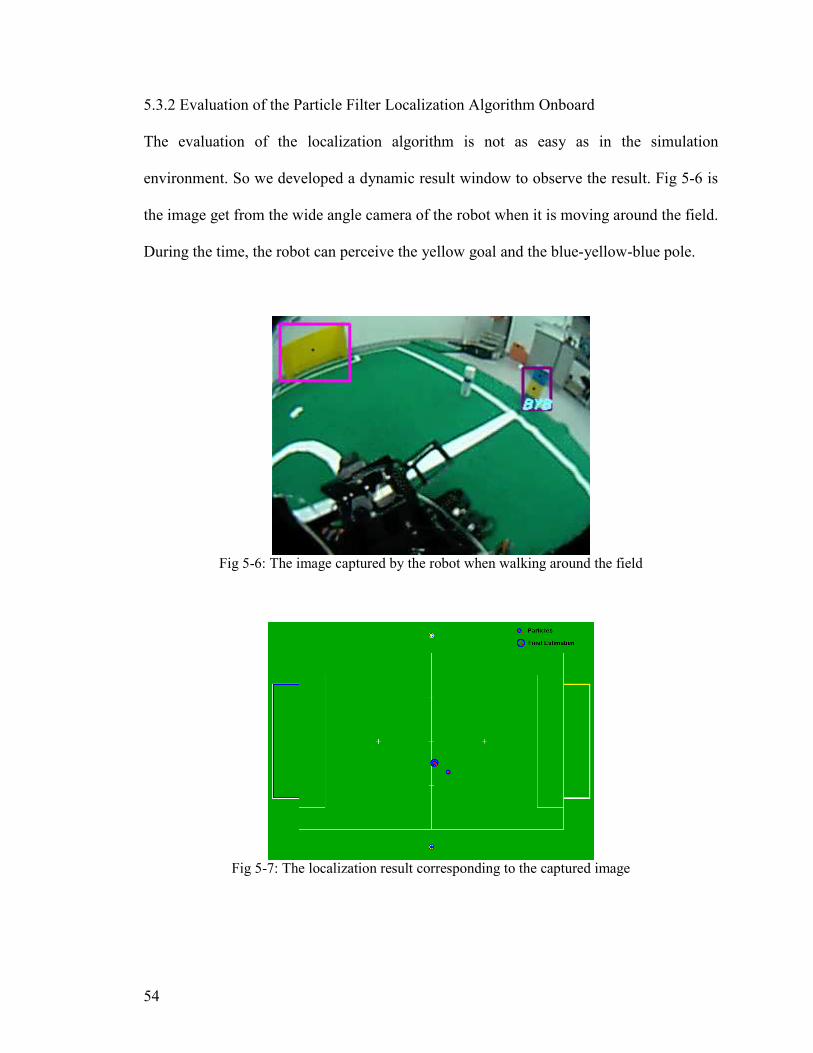
54

5.3.2 Evaluation of the Particle Filter Localization Algorithm Onboard

The evaluation of the localization algorithm is not as easy as in the simulation

environment. So we developed a dynamic result window to observe the result. Fig 5-6 is

the image get from the wide angle camera of the robot when it is moving around the field.

During the time, the robot can perceive the yellow goal and the blue-yellow-blue pole.

Fig 5-6: The image captured by the robot when walking around the field

Fig 5-7: The localization result corresponding to the captured image

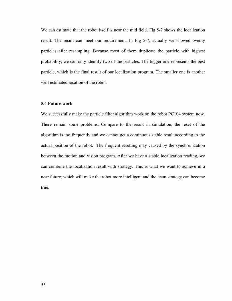
55

We can estimate that the robot itself is near the mid field. Fig 5-7 shows the localization

result. The result can meet our requirement. In Fig 5-7, actually we showed twenty

particles after resampling. Because most of them duplicate the particle with highest

probability, we can only identify two of the particles. The bigger one represents the best

particle, which is the final result of our localization program. The smaller one is another

well estimated location of the robot.

5.4 Future work

We successfully make the particle filter algorithm work on the robot PC104 system now.

There remain some problems. Compare to the result in simulation, the reset of the

algorithm is too frequently and we cannot get a continuous stable result according to the

actual position of the robot. The frequent resetting may caused by the synchronization

between the motion and vision program. After we have a stable localization reading, we

can combine the localization result with strategy. This is what we want to achieve in a

near future, which will make the robot more intelligent and the team strategy can become

true.

56

CHAPTER VI

CONCLUSION

In this thesis we addressed several aspects of the humanoid robot localization based on

particle filter algorithm in the robot soccer game. We aim to develop a localization

scheme that can realize the robot self-localization efficiently and accurately. We employ

the particle filter algorithm to perform the robot self-localization. To implement the

algorithm on the robot, we developed the motion model and vision model for the robot

based on the particular configuration and improved the particle filter algorithm.

After the introduction to the localization problem and the particle filter, we developed the

motion model and the vision model for our RO-PE VI humanoid robot. We developed a

very simple odometry for the humanoid robot through kinematics. This is a very efficient

method and it can provide a better result than simply employ a Gaussian noise to model

the robot displacement. The vision model we developed is based on the characteristic of

the fish-eye lens. We verified the result through experiment and it shows that the vision

model can provide accurate information for our localization algorithm. Adopting the

traditional way to build a vision model, we need to calibrate the camera, undistorted the

image, use the coordinate transformations and finally get the respective position of the

landmarks. The computation for the traditional way is very expensive.

57

Before implementing the whole algorithm on the robot, we simulated the algorithm

utilizing MatLab™. This is to verify and tune the particle filter algorithm. We came out a

new particle reset algorithm, to increase the variance due to the limited number of

particles we employed. After several experiments on global localization, position tracking

and kidnapped problem, the resetting algorithm works well and the localization results

are within our expectation. Based on the particle reset mechanism, we developed a new

switching particle filter algorithm to improve the efficiency of the particle filter.

After having the motion model, vision model and efficient particle filter algorithm, we

start to implement the whole algorithm on the robot. To fit the algorithm into a real time

system, we changed the particle filter to a parallel structure, and improved the efficiency

of resampling. Finally the algorithm can run without problem on the onboard AMD

500MHz PC104, and other programs are still can run independent without the particle

filter algorithm.

We developed the localization algorithm from scratch for the RO-PE VI. But there are

many improvements can be done in the future. We did not include the line information on

the field, which will definitely increase the accuracy of the localization algorithm. A few

parameters can be fine tuned to improve the localization result. We can pack the particle

filter to a more dependent function, and easy to implement. In summary, we developed a

new switching particle filter algorithm and it works well. In the future, we still need to

improve the performance of the algorithm on the real platform.

58

REFERENCES

1. Thrun, S., W. Burgard, and D. Fox, Probabilistic Robotics. 2005: MIT Press.

2. Fox, D., et al., Particle filters for mobile robot localization. Sequential Monte

Carlo Methods in Practice. 2001: Springer.

3. Flury, T. and N. Shephard, Bayesian inference based only on simulated

likelihood: particle filter analysis of dynamic economic models. 2008.

4. Röfer, T. and M. Jungel, Vision-Based Fast and Reactive Monte-Carlo

Localization, in IEEE International Conference on Robotics and Automation.

2003: Taipei, Taiwan.

5. Chew, C.-M., et al., Team Description 2009 for Team RO-PE. 2009, National

University of Singapore.

6. Ng, C.L., Machine Vision System and Localization For Soccer-Playing Humanoid

Robots, in Mechanical Engineering 2008, National University of Singapore:

Singapore.

7. Ma, C., Motion Control for Football-Playing Humanoid Robots, in Mechanical

Engineering. 2008, National University of Singapore: Singapore.

8. Li, R., Motion Control and Simulation for Football-Playing Humanoid Robot, in

Mechanical Engineering. 2009, National University of Singapore: Singapore.

9. Cox, I.J., Blanche-an experiment in guidance and navigation of an autonomous

robot vehicle. IEEE Transactions on Robotics and Automation, 1991. 7(2): p. 12.

10. Borenstein, J., et al., Mobile robot positioning: Sensors and techniques. Journal of

Robotic Systems, 1997.

11. Gutmann, J. and D. Fox, An experimental comparison of localization methods

continued, in Intelligent Robots and System. 2002.

12. Thrun, S., et al., Robust Monte Carlo localization for mobile robots. Artificial

Intelligence, 2001. 128.

13. Filliat, D., Map-based navigation in mobile robots: I. A review of localization

strategies. Cognitive Systems Research, 2003. 243(282).

14. Rekleitis, I.M., Cooperative localization and multi-robot exploration, in

Computer Science. 2003, McGill University.

15. Schulenburg, E., T. Weigel, and A. Kleiner, Self-Localization in Dynamic

Environments based on Laser and Vision Data, in IROS 2003.

16. Marques, C. and P. Lima, A localization method for a soccer robot using a vision-

based omni-directional sensor. RoboCup-2000: Robot Soccer World Cup IV.

2001.

17. Enderle, S., et al., Vision-based localization in robocup environments. RoboCup-

2000: Robot Soccer World Cup IV 2001.

18. S Enderle, D.F., S Sablatnog, GK, Vision-based localization in robocup

environments. RoboCup-2000: Robot Soccer World Cup IV 2001.

19. Fox, D., Markov Localization: A probabilistic framework for mobile robot

localization and navigation, in Institute of Computer Science III. 1998, University

of Bonn, Germany.

20. Lenser, S. and M. Veloso, Sensor Resetting Localization for Poorly Modelled

Mobile Robots, in IEEE International Conference on Robotics and Automation.

2000.

59

21. Röfer, T., T. Laue, and D. Thomas, Particle-Filter-Based Self-localization Using

Landmarks and Directed Lines, in RoboCup 2005: Robot Soccer World Cup IX.

2006, Springer Berlin / Heidelberg. p. 608-615.

22. Röfer, T. and M. Jungel, Fast and robust edge-based localization in the sony

four-legged robot league, in RoboCup 2003: Robot Soccer World Cup VII. 2004,

Springer Berlin / Heidelberg. p. 262-273.

23. Sridharan, M., G. Kuhlmann, and P. Stone, Practical Vision-Based Monte Carlo

Localization on a Legged Robot, in IEEE International Conference on Robotics

and Automation. 2005: Barcelona, Spain.

24. Göhring, D. and H.-D. Burkhard, Multi Robot Object Tracking and Self

Localization Using Visual Percept Relations, in International Conference on

Intelligent Robots and Systems. 2006: Beijing.

25. Stronger, D. and P. Stone, A Comparison of Two Approaches for Vision and Self-

Localization on a Mobile Robot, in International Conference on Robotics and

Automation. 2007: Rome.

26. Laue, T. and T. Röfer, Particle Filter-based State Estimation in a Competitive

and Uncertain. Environment, in International Workshop on Embedded Systems.

2007.

27. Friedmann, M., et al., Reusable Architecture and tools for teams of lightweight

heterogeneous robots, in IFAC Workshop on multivehicle systems. 2006.

28. Strasdat, H., M. Bennewitz, and S. Behnke, Multi-cue Localization for Soccer

Playing Humanoid Robots. 2007.

29. Woodman, O.J., An introduction to inertial navigation. 2007, University of

Cambridge.

30. Cho, S.Y., C.G. Park, and G.I. Jee, Measurement System of Walking Distance

Using Low-cost Accelerometers, in Asian Control Conference. 2002: Singapore.

31. Jüngel, M., A Vision System for RoboCup, in Institut für Informatik. 2004,

Humboldt-Universität zu Berlin.

32. Rekleitis, I.M., A particle filter tutorial for mobile robot localization, in

International Conference on Robotics and Automation. 2003.

33. Schwalbe, E. Geometric modelling and calibration of fisheye lens camera

systems. in International Society for Photogrammetry and Remote Sensing. 2005.

34. Birchfield, S., An introduction to projective geometry (for computer vision). 1998,

Stanford university.

35. Laue, T. and T. Röfer, Pose Extraction from Sample Sets in Robot Self-

Localization – A Comparison and a Novel Approach, in European Conference on

Mobile Robots. 2009.

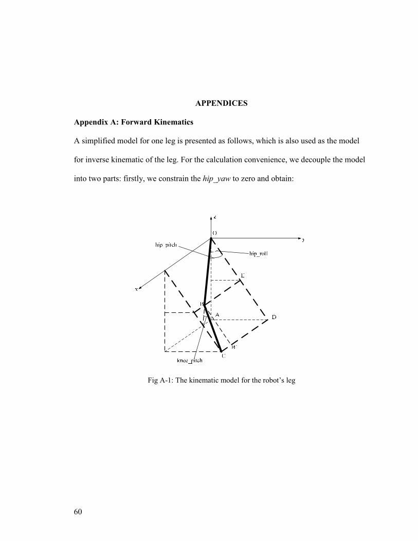
60

APPENDICES

Appendix A: Forward Kinematics

A simplified model for one leg is presented as follows, which is also used as the model

for inverse kinematic of the leg. For the calculation convenience, we decouple the model

into two parts: firstly, we constrain the hip_yaw to zero and obtain:

Fig A-1: The kinematic model for the robot’s leg

61

Fig A-2: Side plane view for showing the hip pitch and knee pitch

Fig A-3: Front plane view for showing the hip roll

( )( )

( )( )

( ) ( )

cos _

cos _ _

cos _

sin _

sin _ sin _ _

OE OB hip pitch

ED BC hip pitch knee pitch

OD OE ED

z OA OD hip roll

y AD OD hip roll

x CD CB B D OB hip pitch BC hip pitch knee pitch

=

= −

= +

= =

= =

′ ′= = + = + −

62

Second part, we take hip_yaw into consideration. This is a projection of the leg to the x-y

plane.

θ

Fig A-4: Coordinate transformation when there is a hip yaw motion

We can obtain:

_

cos sin cos sin

sin cos sin cos

'

hip yaw

x x x y

y y x y

z z

θ

θ θ θ θθ θ θ θ

=

′ − − = = ′ +

=

From the kinematic model, we can get the relative position of every step. After building

the model of the legs, we need to calculate the distance between the two feet when it is

double support phase. Every step, we can identify the stance leg and swing leg through

the length of each leg. During the double support phase we calculate the position of each

foot respectively. For example, the left leg is the stance leg and the right leg is the swing

leg. When the right foot just touches the ground, we update the odometry:

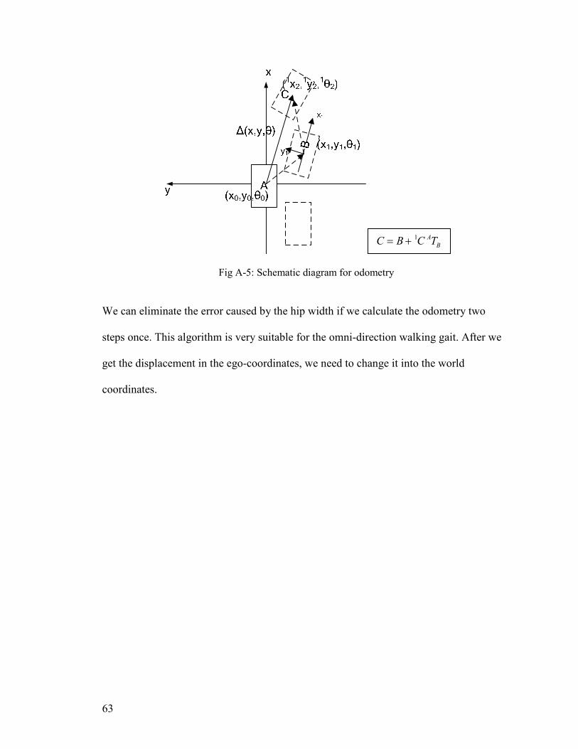
63

Fig A-5: Schematic diagram for odometry

We can eliminate the error caused by the hip width if we calculate the odometry two

steps once. This algorithm is very suitable for the omni-direction walking gait. After we

get the displacement in the ego-coordinates, we need to change it into the world

coordinates.

1 A

BC B C T= +

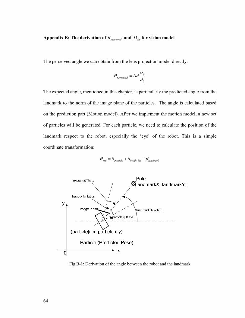
64

Appendix B: The derivation of perceivedθ and objD for vision model

The perceived angle we can obtain from the lens projection model directly.

0

0

perceived dd

αθ = ∆

The expected angle, mentioned in this chapter, is particularly the predicted angle from the

landmark to the norm of the image plane of the particles. The angle is calculated based

on the prediction part (Motion model). After we implement the motion model, a new set

of particles will be generated. For each particle, we need to calculate the position of the

landmark respect to the robot, especially the ‘eye’ of the robot. This is a simple

coordinate transformation:

exp particle head hip landmarkθ θ θ θ+= + −

Fig B-1: Derivation of the angle between the robot and the landmark

65

To compare the differences between predicted angle and the actual sensed angle, we need

to abstract the information contained in the image though the lens projection model. As

we know the real size of the landmark, and we can get the size of the landmark on the

image, it is not difficult to calculate the object distance through the lens projection model.

.( ).a constantd

α∆=

∆

Because the robot height is almost 60cm, and the height of the pole is 60cm. And the pole

is perpendicular to the ground, and we also can consider that the robot is always

perpendicular to the ground. As shown in the Fig 3-8, we can consider that the landmark

AB is perpendicular to the straight line of sight OA. Most of the time ∆α is a small angle,

so we obtain:

landmark objL D α= ∆

It is known that the distance between CCD array elements is a constant. The number of

pixels we can count from the image taken by the camera. We have:

pixeld nd∆ =

Now from the equations we have, we can calculate the Distance from the camera to the

landmark, which is almost the same as the distance from the feet of the robot to the

bottom of the pole.

landmark landmarkobj

pixel

L LD

and nA= =

66

Appendix C: Essential MatLab™ code for simulation

%Motion Model and Noise for i = 1:N Dx = odom_x + 0.05 * 2 *(rand + rand - 1); Dy = odom_y + 0.05* 1 *(rand + rand - 1); Dtheta = odom_theta + 30 * D2R *(rand + rand - 1); particle(i).x = particle(i).x + Dx * cos(particle(i).theta) + Dy * sin(particle(i).theta); particle(i).y = particle(i).y + Dx * sin(particle(i).theta) - Dy * cos(particle(i).theta); particle(i).theta = particle(i).theta + Dtheta; particle(i).reset = 1; if particle(i).x > FIELD_LENGTH particle(i).x = FIELD_LENGTH; elseif particle(i).x < 0 particle(i).x = 0; end if particle(i).y > FIELD_WIDTH particle(i).y = FIELD_WIDTH; elseif particle(i).y < 0 particle(i).y = 0; end if particle(i).theta > pi particle(i).theta = particle(i).theta - 2 * pi; elseif particle(i).theta < -pi particle(i).theta = particle(i).theta + 2 * pi; end end

%Vision Model angleArr.x = [YELLOW_GOAL_N_X YELLOW_GOAL_S_X BLUE_GOAL_N_X BLUE_GOAL_S_X YBY_POLE_X BYB_POLE_X]; angleArr.y = [YELLOW_GOAL_N_Y YELLOW_GOAL_S_Y BLUE_GOAL_N_Y BLUE_GOAL_S_Y YBY_POLE_Y BYB_POLE_Y]; dist = 0; for j = 1:6 angleArr.perceived(j) = atan2(angleArr.y(j)-y, angleArr.x(j)-x)-theta; distArr.perceived(j) = sqrt((angleArr.y(j) - y)^2 + (angleArr.x(j) - x)^2); end %Update the weight of all the particles for i = 1:N for j = 1:6 if angleArr.perceived(j) > pi angleArr.perceived(j) = angleArr.perceived(j) - 2 * pi;

67

elseif angleArr.perceived(j) < -pi angleArr.perceived(j) = angleArr.perceived(j) + 2 * pi; end if (angleArr.perceived(j)<(67*D2R)) && (angleArr.perceived(j)> (-67*D2R)) angleArr.exp(j) = atan2(angleArr.y(j) - particle(i).y, angleArr.x(j) - particle(i).x) -particle(i).theta; angleArr.delta(j) = angleArr.exp(j) - angleArr.perceived(j); %This is to simplify the angle to (-180,180) if angleArr.delta(j) > pi angleArr.delta(j) = angleArr.delta(j) - 2 * pi; elseif angleArr.delta(j) < -pi angleArr.delta(j) = angleArr.delta(j) + 2 * pi; end u = angleArr.delta(j)/(pi/12); belief = 0.39894228 * exp( -0.5 * u * u); particle(i).w = particle(i).w * belief; distArr.exp(j) = sqrt((angleArr.y(j) - particle(i).y)^2 + (angleArr.x(j) - particle(i).x)^2 ); if distArr.exp(j)~=0 if distArr.perceived(j) > sqrt(FIELD_WIDTH^2 + FIELD_LENGTH^2) distArr.perceived(j) = sqrt(FIELD_WIDTH^2 + FIELD_LENGTH^2); end if distArr.perceived(j) >= distArr.exp(j) distArr.delta(j) = (distArr.perceived(j) - distArr.exp(j)) / distArr.exp(j); elseif distArr.perceived(j) < distArr.exp(j) distArr.delta(j) = (distArr.exp(j) - distArr.perceived(j)) / distArr.perceived(j); end u = distArr.delta(j); belief = 0.39894228 * exp( -0.5 * u * u); particle(i).w = particle(i).w * belief; if distArr.delta(j)~=0 && distArr.delta(j)<distMinErr && abs(angleArr.delta(j))<angleMinErr particle(i).reset = 0; end end else angleArr.exp(j)=0; angleArr.delta(j)=0; end end

68

end

%Resample sumWeight = 0; accSum = 0; for i = 1:N sumWeight = particle(i).w + sumWeight; accSum(i) = sumWeight; end a = sumWeight * rand(N,1); a = sort(a); a(N + 1) = sumWeight; for i = 1:N particle(i).w = particle(i).w/sumWeight; end indexParticle = 1; for i = 1:N indexParticle(i)=1; end i = 1; j = 1; while (i <=N) && (j <= N) if (a(i) < accSum(j)) indexParticle(i)=j; i=i+1; else j=j+1; end end temp = particle; for i = 1:N sub = indexParticle(i); temp(i) = particle(sub); end for i = 1:N particle(i) = temp(i); end