selected topics on applications of graph spectra
TRANSCRIPT

Zbornik radova 14 (22)
SELECTED TOPICS ONAPPLICATIONS OFGRAPH SPECTRA
Editors:
Dragos Cvetkovic and Ivan Gutman
Matematicki institut SANU

Izdavaq: Matematiqki institut SANU, Beograd, Kneza Mihaila 36
serija: Zbornik radova, knjiga 14 (22)
Za izdavaqa: Bogoljub Stankovi�, glavni urednik serije
Urednici sveske: Dragox Cvetkovi� i Ivan Gutman, kao gosti
Tehniqki urednik: Dragan Blagojevi�
Xtampa: “Akademska izdanja”, Zemun
Xtampanje zavrxeno januara 2011.
CIP – Katalogizacija u publikaciji
Narodna biblioteka Srbije, Beograd
519.17(082)
SELECTED Topics on Applications of Graph
Spectra / editors Dragos Cvetkovic and Ivan
Gutman. - Beograd : Matematicki institut
SANU, 2011 (Zemun : Akademska izdanja). - 174
str. : graf. prikazi, tabele ; 24 cm. -
(Zbornik radova / Matematicki institut SANU ;
knj. 14 (22))
Prema Predgovoru ovo je dopunjeno izd.
publikacije “Applications of Graph Spectra”
iz 2009. Tiraz 500. - Str 4-5: Preface /
Dragos Cvetkovic, Ivan Gutman. - Str. 6-7:
From Preface to volume 13(21) / Dragos
Cvetkovic, Ivan Gutman. - Bibliografija uz
svaki rad.
ISBN 978-86-80593-44-9
1. Cvetkovic, Dragos, 1941– [urednik]
[autor dodatnog teksta] 2. Gutman, Ivan,
1947– [urednik] [autor dodatnog teksta]
a) Teorija grafova – Zbornici
COBISS.SR-ID 181188876

PREFACE
The volume 13(21) of the Collection of Papers (Zbornik radova) with the titleApplications of Graph Spectra appeared in 2009 and was soon out of print. Weproposed to the Mathematical Institute of the Serbian Academy of Sciences andArts to publish a second edition, but the Editorial Board decided to publish a newvolume on the same subject with a similar title and with the same guest editors.We have chosen the title Selected Topics on Applications of Graph Spectrafor the new volume.The purpose of this volume and of the previous volume is to draw the attention
of the mathematical community to the rapidly growing applications of the theoryof graph spectra. Besides classical and well documented applications to Chemistryand Physics, we are witnesses of the appearance of graph eigenvalues in ComputerScience in various investigations. There are also applications in several other fieldslike Biology, Geography, Economics, and Social Sciences.A part of the Preface to volume 13(21) is reproduced below.The new volume contains improved, modified, and extended versions of all chap-
ters from volume 13(21) as well as the following two new chapters:
Spectral Techniques in Complex Networks (S. Gago),Applications of Graph Spectra in Quantum Physics (D. Stevanovic).
The old chapters have been technically improved including the correction of no-ticed typos and other mistakes. In addition the following changes have been made.
Applications of Graph Spectra: An Introduction to the Literature(D. Cvetkovic). Some new references have been added and the presentation ofsome parts is improved.
Multiprocessor Interconnection Networks (D. Cvetkovic, T. Davidovic).New proofs of main theorems are given and the data for some interesting multipro-cessor interconnection networks are better presented.
Hyperenergetic and Hypoenergetic Graphs (I. Gutman). This is a newtext, with a slight overlap to the chapter Selected Topics from the Theory of GraphEnergy: Hypoenergetic Graphs, (S. Majstorovic, A. Klobucar, I. Gutman), thatappeared in volume 13(21).
Nullity Of Graphs: An Updated Survey (I. Gutman, B. Borovicanin). Thechapter Nullity of Graphs, (I. Gutman, B. Borovicanin), is extended by surveyinga number of recently published results, and by updating the bibliography.
The Estrada Index: An Updated Survey (I. Gutman, H. Deng, S. Raden-kovic). The chapter The Estrada Index, (H. Deng, S. Radenkovic, I. Gutman), isextended by surveying a number of recently published results, and by updating thebibliography.
For some more information on these Chapters see Preface to volume 13(21).
The new chapter by S. Gago is about networks with a great number of verticescalled complex networks. Most physical, biological, chemical, technological, andsocial systems have a network structure. Examples of complex networks range

from cell biology to epidemiology or to the Internet. The rich information aboutthe topological structure and diffusion processes can be extracted from the spectralanalysis of the corresponding networks.The new chapter by D. Stevanovic explains that graph spectra are closely related
to many applications in quantum physics: a network of quantum particles withfixed couplings can be modelled by an underlying graph, the Hamiltonian of suchsystem can be approximated either by the adjacency or the Laplacian matrix ofthat graph, and then quite a few problems can be posed in terms of the eigenvaluesof the graph. One particular problem of interest to quantum physicists is addressed:the existence of perfect state transfer in networks of spin −1/2 particles.
Authors’ affiliations:
D. Cvetkovic, T. Davidovic, Mathematical Institute of the Serbian Academy ofSciences and Arts, Belgrade, Serbia;S. Gago, Technical University of Catalonia, Barcelona, Spain;D. Stevanovic, Faculty of Science, University of Nis;B. Borovicanin, I. Gutman, S. Radenkovic, Faculty of Science, University of
Kragujevac, Kragujevac, Serbia;H. Deng, College of Mathematics and Computer Science, Hunan Normal Univer-
sity, Changsha, P.R. China.
Author’s e-mail addresses:
Bojana Borovicanin, [email protected] Cvetkovic, [email protected] Davidovic, [email protected] ac.rsHanyuan Deng, [email protected] Gago, [email protected] Gutman, [email protected] Radenkovic, [email protected] Stevanovic, [email protected]
The Guest Editors and some of the authors (B. Borovicanin, D. Cvetkovic, T.Davidovic, I. Gutman, S. Radenkovic, D. Stevanovic) are grateful to the SerbianMinistry of Science and Technological Development for the support through thegrant No. 144015G (Graph Theory and Mathematical Programming with Applica-tions to Chemistry and Engineering).
Belgrade and Kragujevac, 2010Guest Editors:Dragos CvetkovicIvan Gutman

FROM PREFACE TO VOLUME 13(21)
The purpose of this volume is to draw the attention of mathematical communityto rapidly growing applications of the theory of graph spectra. Besides classical andwell documented applications to Chemistry and Physics, we are witnesses of the ap-pearance of graph eigenvalues in Computer Science in various investigations. Thereare also applications in several other fields like Biology, Geography, Economics andSocial Sciences. A monograph with a comprehensive treatment of applications ofgraphs spectra is missing at the present.The present book contains five chapters: an introductory chapter with a survey
of applications by representative examples and four case studies (one in ComputerScience and three in Chemistry).We quote particular chapters and indicate their contents.
Applications of Graph Spectra: An Introduction to the Literature(D. Cvetkovic). This introductory text provides an introduction to the theory ofgraph spectra and a short survey of applications of graph spectra. There are foursections: 1. Basic notions, 2. Some results, 3. A survey of applications, 4. Selectedbibliographies on applications of the theory of graph spectra.
Multiprocessor Interconnection Networks (D. Cvetkovic, T. Davidovic).Well-suited multiprocessor interconnection networks are described in terms of thegraph invariant called tightness which is defined as the product of the numberof distinct eigenvalues and maximum vertex degree. Load balancing problem ispresented.
Selected Topics from the Theory of Graph Energy: HypoenergeticGraphs (S. Majstorovic, A. Klobucar, I. Gutman). The energy E of a graphG is the sum of the absolute values of the eigenvvalues of G. The motivationfor the introduction of this invariant comes from Chemistry, where results on Ewere obtained already in the 1940’s. The chemical background of graph energy isoutlined in due detail. Then some fundamental results on E are given.A graph G with n vertices is said to be “hypoenergetic” if E(G) < n. In the
main part of the chapter results on graph energy, pertaining to the inequalitiesE(G) < n and E(G) ≥ n are presented. Most of these were obtained in the lastfew years.
Nullity of Graphs (B. Borovicanin, I. Gutman). The nullity η of a graph G isthe multiplicity of the number zero in the spectrum of G. In the 1970s the nullityof graphs was much studied in Chemistry, because for certain types of molecules,η = 0 is a necessary condition for chemical stability. The chemical background ofthis result is explained in a way understandable to mathematicians. Then the mainearly results on nullity are outlined.In the last 5–10 years there is an increased interest to nullity in mathematics, and
some 10 papers on this topic appeared in the mathematical literature. All theseresults are outlined too.
The Estrada Index (H. Deng, S. Radenkovic, I. Gutman). If λi, i = 1, 2, . . . , n,are the eigenvalues of the graph G, then the Estrada index EE of G is the sum of

the terms exp(λi). This graph invariant appeared for the first time in year 2000,in a paper by Ernesto Estrada, dealing with the folding of protein molecules. Sincethen a remarkable number of other chemical and non-chemical applications of EEwere communicated.The mathematical studies of the Estrada index started only a few years ago.
Until now a number of lower and upper bounds were obtained, and the problem ofextremal EE for trees solved. Also, a number of approximations and correlationsfor EE were put forward, valid for chemically interesting molecular graphs.All relevant results on the Estrada index are presented in the chapter.
Manuscripts have been submitted in January 2009 and revised in April 2009.
Belgrade and Kragujevac, 2009Guest Editors:Dragos CvetkovicIvan Gutman

Contents
Dragos Cvetkovic:
APPLICATIONS OF GRAPH SPECTRA:AN INTRODUCTION TO THE LITERATURE 9
Dragos Cvetkovic and Tatjana Davidovic:
MULTIPROCESSOR INTERCONNECTION NETWORKS 35
Silvia Gago:
SPECTRAL TECHNIQUES IN COMPLEX NETWORKS 63
Dragan Stevanovic:
APPLICATIONS OF GRAPH SPECTRA IN QUANTUM PHYSICS 85
Ivan Gutman:
HYPERENERGETIC AND HYPOENERGETIC GRAPHS 113
Ivan Gutman and Bojana Borovicanin:
NULLITY OF GRAPHS: AN UPDATED SURVEY 137
Ivan Gutman, Hanyuan Deng, and Slavko Radenkovic:
THE ESTRADA INDEX: AN UPDATED SURVEY 155


Dragos Cvetkovic
APPLICATIONS OF GRAPH SPECTRA:
AN INTRODUCTION TO THE LITERATURE
Abstract. We give basic definitions and some results related to thetheory of graph spectra. We present a short survey of applicationsof this theory. In addition, selected bibliographies on applications toparticular branches of science are given.
Mathematics Subject Classification (2010): 05C50, 05C90, 01A90
Keywords : graph spectra, application, bibliography, chemistry,physics, computer science

Contents
1. Basic notions 102. Some results 123. A survey of applications 153.1. Chemistry 153.2. Physics 163.3. Computer science 163.4. Mathematics 183.5. Other sciences 194. Selected bibliographies on applications of the theory of graph spectra 224.1. Chemistry 224.2. Physics 284.3. Computer science 304.4. Engineering 324.5. Biology 334.6. Economics 33
This is an introductory chapter to our book. We start with basic definitionsand present some results from the theory of graph spectra. A short survey ofapplications of this theory is presented. Selected bibliographies on applications toparticular branches of science are given in the sequel.
The plan of the chapter is as follows.Section 1 presents basic definitions related to the theory of graph spectra. Some
selected results, which will bi used in other chapters, are given in Section 2. Ashort survey of applications of graph eigenvalues is contained in Section 3. Section4 contains selected bibliographies of books and papers which are related to appli-cations of the theory of graph spectra in Chemistry, Physics, Computer Science,Engineering, Biology and Economics.
1. Basic notions
A graph G = (V,E) consists of a finite non-empty set V (the vertex set of G),and a set E (of two elements subsets of V , the edge set of G). We also write V (G)(E(G)) for the vertex (resp. edge) set of G. The number of elements in V (G),denoted by n (= |V (G)|), is called the order of G. Usually, we shall assume thatV (G) = {1, 2, . . . , n}.
Let eij be the edge connecting vertices i and j. The set {ei1j1 , ei2j2 , . . . , eikjk}of distinct edges, such that i = i1, j1 = i2, j2 = i3, . . . , jk = j, is called path (oflength k) connecting vertices i and j. The length of the shortest path connectingi and j is called the distance between these two vertices. The maximum distancebetween any two vertices in G is called the diameter of G, and it is denoted by D.If there exists a path between any two vertices in G, then G is connected ; otherwiseit is disconnected.
APPLICATIONS OF GRAPH SPECTRA: AN INTRODUCTION TO THE LITERATURE 11
Two vertices are called adjacent (or neighbors) if they are connected by an edge;the corresponding relation between vertices is called the adjacency relation. Thenumber of neighbors of a vertex i, denoted by di, is its vertex degree. The maximumvertex degree (of G) is denoted by Δ. A graph in which all vertex degrees are equalto r is regular of degree r (or r-regular, or just regular if r is unimportant).
The adjacency matrix A is used to represent the adjacency relation, and so thegraph G itself. The element aij of the adjacency matrix A is equal to 1 if verticesi and j are adjacent, and 0 otherwise.
The characteristic polynomial det(xI − A) of the adjacency matrix A (of G) iscalled the characteristic polynomial of G, and is denoted by PG(x). The eigenvaluesof A (i.e., the zeros of det(xI−A)), and the spectrum of A (which consists of the neigenvalues) are also called the eigenvalues and the spectrum of G, respectively. Theeigenvalues of G are usually denoted by λ1, λ2, . . . , λn; they are real because A issymmetric. Unless we indicate otherwise, we shall assume that λ1 � λ2 � · · · � λn.We also use the notation λi = λi(G) for i = 1, 2, . . . , n. The largest eigenvalue, i.e.,λ1, is called the index of G.
If λ is an eigenvalue of G, then a non-zero vector x ∈ Rn, satisfying Ax = λx,
is called an eigenvector of A (or of the labeled graph G) for λ; it is also called aλ-eigenvector. The relation Ax = λx can be interpreted in the following way: ifx = (x1, x2, . . . , xn)
T , then for any vertex u we have λxu =∑
v∼u xv, where thesummation is over all neighbours v of u. If λ is an eigenvalue of G, then the set{x ∈ R
n : Ax = λx} is a subspace of Rn, called the eigenspace of G for λ; it isdenoted by E(λ). Such eigenspaces are called eigenspaces of G.
For the index of G, since A is non-negative, there exists an eigenvector whoseall entries are non-negative.
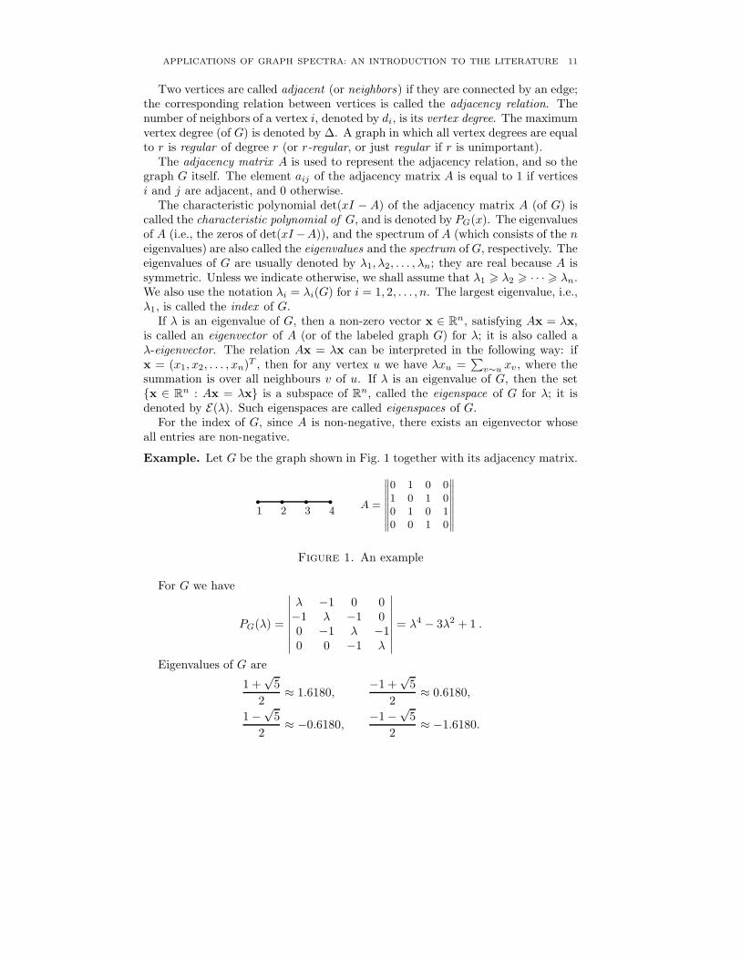
Example. Let G be the graph shown in Fig. 1 together with its adjacency matrix.
� � � �
1 2 3 4A =
∥∥∥∥∥∥∥∥
0 1 0 01 0 1 00 1 0 10 0 1 0
∥∥∥∥∥∥∥∥
Figure 1. An example
For G we have
PG(λ) =
∣∣∣∣∣∣∣∣
λ −1 0 0−1 λ −1 00 −1 λ −10 0 −1 λ
∣∣∣∣∣∣∣∣
= λ4 − 3λ2 + 1 .
Eigenvalues of G are
1 +√5
2≈ 1.6180,
−1 +√5
2≈ 0.6180,
1−√5
2≈ −0.6180,
−1−√5
2≈ −1.6180.

12 DRAGOS CVETKOVIC
The following vector x = (1, λ, λ2 − 1, λ3 − 2λ)T is a λ-eigenvector of G. �
Besides the spectrum of the adjacency matrix of a graph G we shall considerthe spectrum of another matrix associated with G. The matrix L = D−A, whereD = diag(d1, d2, . . . , dn) is the diagonal matrix of vertex degrees, is known as theLaplacian of G. The matrix L is positive semi-definite, and therefore its eigenval-ues are non-negative. The least eigenvalue is always equal to 0; the second leasteigenvalue is also called the algebraic connectivity of of G [Fie].
The basic reference for the theory of graph spectra is the book [CvDSa]. Otherbooks on graph spectra include [CvDGT], [CvRS1], [CvRS3], [CvRS4]. For anynotion, not defined here, the reader is referred to [CvRS4] or [CvDSa].
As usual, Kn, Cn, Sn and Pn denote respectively the complete graph, the cycle,the star and the path on n vertices; Kn1,n2 denotes the complete bipartite graphon n1 + n2 vertices.
A tree is a connected graph without cycles. A connected graph with n verticesand n edges is a unicyclic graph. It is called even (odd) if its unique cycle is even(resp. odd). A dumbbell is the graph obtained from two disjoint cycles by joiningthem by a path.
The complement of a graph G is denoted by G, while mG denotes the union ofm disjoint copies of G.
For v ∈ V (G), G − v denotes the graph obtained from G by deleting v, and alledges incident with it. More generally, for U ⊆ V (G), G− U is the subgraph of Gobtained from G by deleting all vertices from U and edges incident to at least onevertex of U ; we also say that GU is induced by the vertex set V (G) \ U .
The join G∇H of (disjoint) graphs G and H is the graph obtained from G andH by joining each vertex of G with each vertex of H . For any graph G, the coneover G is the graph K1∇G.
The line graph L(H) of any graph H is defined as follows. The vertices ofL(H) are the edges of H and two vertices of L(H) are adjacent whenever thecorresponding edges of H have a vertex of H in common.
A set of disjoint edges in a graph G is called a matching. A set of disjoint edgeswhich cover all vertices of the graph is called an 1-factor of G.
2. Some results
We present here some known results from the theory of graph spectra that willbe used in other chapters.
In graph theory and in the theory of graph spectra, some special types of graphsare studied in detail and their characteristics are well known and summarized inthe literature (see, for example, [CvDSa]). Here, we will survey some of them.
Recall, Kn is a complete graph, i.e., a graph with each two vertices connectedby an edge (so, the number of edges is equal to
(n2
)). The spectrum of Kn consists
of m = 2 distinct eigenvalues: λ1 = n−1 which is a simple eigenvalue, and λi = −1for i = 2, . . . , n.
A path Pn is a tree on n vertices (and n − 1 edges) without vertices of degreegreater than two. Two “ending” vertices (for n � 2) have degree one, while the rest

APPLICATIONS OF GRAPH SPECTRA: AN INTRODUCTION TO THE LITERATURE 13
of them (the internal vertices) have degree two. A spectral characteristic of pathsis that they have all distinct eigenvalues. In fact, the spectrum of Pn consists ofthe following eigenvalues: 2 cos π
n+1 i, i = 1, 2, . . . , n.The Cn is a 2-regular connected graph. It contains the following eigenvalues:
2 cos 2πn i, i = 0, 1, . . . , n − 1. It has m = �n
2 � + 1 distinct eigenvalues. Here �x�denotes the largest integer smaller than or equal to x.
The star Sn is a tree having a vertex (central vertex) which is adjacent to allremaining vertices (all of them being of degree one). Each star on n � 3 verticeshas m = 3 distinct eigenvalues. It contains the following eigenvalues: ±√
n− 1which are both simple, and λi = −1 for i = 2, . . . , n− 1.
A complete bipartite graph Kn1,n2 consists of n1 + n2 vertices divided into twosets of the cardinalities n1 and n2 with the edges connecting each vertex from oneset to all the vertices in the other set. This means that the number of edges isn1n2. In particular, Sn = K1,n−1. More generally, bipartite graphs consist of twosets of vertices with the edges connecting a vertex from one set to a vertex in theother set. The spectrum of Kn1,n2 (for n1 +n2 � 3) also consists of m = 3 distincteigenvalues (simple eigenvalues ±√
n1n2, and 0 of multiplicity n1 + n2 − 2).In the theory of graph spectra an important role play the graphs with λ1 = 2,
known as Smith graphs. They are well studied, and all of them are given in [CvDSa],on Fig. 2.4, p. 79. There are 6 types of Smith graphs (namely, Cn (n � 3), Wn
(n � 6), S5 H7, H8 and H9 – see also Fig. 2). Four of them are concrete graphs S5,H7, H8 and H9, while the remaining two types (cycles Cn and double-head snakesWn, of order n, can have an arbitrary number of vertices); in Fig. 2 we reproducethose which are not cycles Cn, nor the star S5 = K1,4.
�
�
� � � �
�
�
��
��
��
��Wn
� �
� �
�
�
�
�� ���� ��H7
� � � �
�
� � �
H8
� � �
�
� � � � �
H9
Figure 2. Some Smith graphs
In our study we need also graphs with λ1 < 2. To obtain such graphs, it isenough to study (connected) subgraphs of Smith graphs. By removing verticesout of Smith graphs, we obtain paths Pn, n = 2, 3, . . .; single-head snakes Zn,n = 4, 5, . . ., given in the upper row of Fig. 3 up to n = 7; and the three othergraphs given in the second row of Fig. 3 and denoted by E6, E7 and E8. It isenough to consider only one vertex removal; removing further vertices leads to thegraph already obtained in another way.

14 DRAGOS CVETKOVIC
�
��
�
��
��Z4
�
��
�
���
��Z5
�
��
�
� ���
��Z6
�
��
�
� � ���
��Z7
� �
� �
�
�
�� ���� ��E6
� � �
�
� � �
E7
� � �
�
� � � �
E8
Figure 3. Subgraphs of some Smith graphs
By Theorem 3.13. from [CvDSa] for the diameter D of a graph G we have
(1) D � m− 1,
where m is the number of distinct eigenvalues.The largest eigenvalue λ1 of G and the maximum vertex degree Δ are related in
the following way (cf. [CvDSa, p. 112 and p. 85]):
(2)√Δ � λ1 � Δ.
A graph is called strongly regular with parameters (n, r, e, f) if it has n verticesand is r-regular, and if any two adjacent (non-adjacent) vertices have exactly e(resp. f) common neighbors [CvDSa]. One can show that the number n of verticesof a strongly regular graph is determined by the remaining three parameters. Notethat a complement of a strongly regular graph is also a strongly regular graph.Usually, strongly regular graphs which are disconnected, or whose complementsare disconnected are excluded from considerations (trivial cases). Under this as-sumption, the diameter of a strongly regular graph is always equal to 2, and alsoit has 3 distinct eigenvalues.
A graph is called integral if its spectrum consists entirely of integers. Eacheigenvalue has integral eigenvectors and each eigenspace has a basis consisting ofsuch eigenvectors.
Graphs with a small number of distinct eigenvalues have attracted much atten-tion in the research community.
The number of distinct eigenvalues of a graph is correlated with its symmetryproperty [CvDSa]: the graphs with a small number of distinct eigenvalues are (veryfrequently) highly symmetric. They also have a small diameter, what follows from(1). Let m be the number of distinct eigenvalues of a graph G. Trivial cases arem = 1 and m = 2. If m = 1, all eigenvalues are equal to 0 and G consists of isolatedvertices. In the case m = 2 G consists of, say k � 1 copies of complete graphs ons � 2 vertices (so the distinct eigenvalues are s − 1 (of multiplicity k) and −1 (ofmultiplicity k(s− 1))).
Further, we shall consider only connected graphs. If m = 3 and G is regular,then G is strongly regular (cf. [CvDSa, p. 108]). For example, the well known

APPLICATIONS OF GRAPH SPECTRA: AN INTRODUCTION TO THE LITERATURE 15
Petersen graph (see Fig. 4) is strongly regular with distinct eigenvalues 3, 1,−2 ofmultiplicities 1, 5, 4, respectively.
� �
� �
�
����
����
����
����
� �
� �
�
����
����
����
��
��
Figure 4. The Petersen graph
It is difficult to construct families of strongly regular graphs which contain graphsfor any number of vertices. It could be rather expected that one can find sporadicexamples with nice properties like it appears in the Petersen graph.
There are also some non-regular graphs with three distinct eigenvalues [Dam].Such graphs usually have a vertex adjacent to all other vertices (like in stars), i.e.,they are cones over some other graphs.
Several classes of regular graphs with four distinct eigenvalues are described in[Dam], but the whole set has not been described yet.
3. A survey of applications
In this section we shall give a short survey of applications of the theory of graphspectra.
The applications are numerous so that we cannot give a comprehensive survey inlimited space that we have at the disposal. We shall rather limit ourselves to reviewrepresentative examples of applications so that the reader can get an impression onthe situation but also to become able to use the literature.
The books [CvDSa], [CvDGT] contain each a chapter on applications of grapheigenvalues.
The book [CvRS4] also contains a chapter on applications . There are sectionson Physics, Chemistry, Computer Sciences and Mathematics itself.
We shall first mention applications to Chemistry, Physics, Computer Sciencesand Mathematics itself (we devote a subsection of this section to each). Graphspectra are used in many other branches of science including Biology, Geography,Economics and Social Sciences and the fifth subsection contains some informationabout that. In all fields we are forced to give only examples of applications.
3.1. Chemistry. Motivation for founding the theory of graph spectra has comefrom applications in Chemistry and Physics.
The paper [Huc] is considered as the first paper where graph spectra appearthough in an implicit form. The first mathematical paper on graph spectra [CoSi]was motivated by the membrane vibration problem i.e., by approximative solvingof partial differential equations.
One of the main applications of graph spectra to Chemistry is the application ina theory of unsaturated conjugated hydrocarbons known as the Huckel molecular

16 DRAGOS CVETKOVIC
orbital theory. Some basic facts of this theory are given at the beginning of thechapter “Selected Topics from the Theory of Graph Energy” in this book.
More detail on the Huckel molecular orbital theory the interested reader can find,for example, in books [CvDSa], [Bal], [CoLM], [Dia], [GrGT], [Gut], [GuTr], [Tri].For more references to the Huckel theory as well as to other chemical applicationssee Section 4.
Three separate chapters of this book are devoted to applications in Chemistry.
3.2. Physics. Treating the membrane vibration problem by approximative solvingof the corresponding partial differential equation leads to consideration of eigenval-ues of a graph which is a discrete model of the membrane (see [CvDSa, Chapter 8]).
The spectra of graphs, or the spectra of certain matrices which are closely relatedto adjacency matrices appear in a number of problems in statistical physics (see,for example, [Kas], [Mon], [Per]). We shall mention the so-called dimer problem.
The dimer problem is related to the investigation of the thermodynamic prop-erties of a system of diatomic molecules (“dimers”) adsorbed on the surface of acrystal. The most favorable points for the adsorption of atoms on such a surfaceform a two-dimensional lattice, and a dimer can occupy two neighboring points.It is necessary to count all ways in which dimers can be arranged on the latticewithout overlapping each other, so that every lattice point is occupied.
The dimer problem on a square lattice is equivalent to the problem of enumer-ating all ways in which a chess-board of dimension n × n (n being even) can becovered by 1
2n2 dominoes, so that each domino covers two adjacent squares of the
chess-board and that all squares are so covered.A graph can be associated with a given adsorption surface. The vertices of
the graph represent the points which are the most favorable for adsorption. Twovertices are adjacent if and only if the corresponding points can be occupied bya dimer. In this manner an arrangement of dimers on the surface determines a1-factor in the corresponding graph, and vice versa. Thus, the dimer problem isreduced to the task of determining the number of 1-factors in a graph. Enumera-tion of 1-factors involves consideration of walks in corresponding graphs and grapheigenvalues (see [CvDSa, Chapter 8]).
Not only the dimer problem but also some other problems can be reduced tothe enumeration of 1-factors (i.e. dimer arrangements). The best known is thefamous Ising problem arising in the theory of ferromagnetism (see, for example,[Kas], [Mon]).
The graph-walk problem is of interest in physics not only because of the 1-factor enumeration problem. The numbers of walks of various kinds in a latticegraph appear in several other problems: the random-walk and self-avoiding-walkproblems (see [Kas], [Mon]) are just two examples.
See also Chapter Applications of Graph Spectra in Quantum Physics.
3.3. Computer science. It was recognized in about last ten years that graph spec-tra have several important applications in computer science. Graph spectra appearin internet technologies, pattern recognition, computer vision and in many otherareas. Here we mention applications in treating some of these and other problems.
APPLICATIONS OF GRAPH SPECTRA: AN INTRODUCTION TO THE LITERATURE 17
(See Chapter Multiprocessor Interconnection Networks for applications in design-ing multiprocessor interconnection topologies and Chapter Spectral Techniques inComplex Networks for applications on Internet).
One of the oldest applications (from 1970’s) of graph eigenvalues in ComputerScience is related to graphs called expanders. Avoiding a formal definition, weshall say that a graph has good expanding properties if each subset of the vertexset of small cardinality has a set of neighbors of large cardinality. Expanders andsome related graphs (called enlargers, magnifiers, concentrators and superconcen-trators, just to mention some specific terms) appear in treatment of several prob-lems in Computer Science (for example, communication networks, error-correctingcodes, optimizing memory space, computing functions, sorting algorithms, etc.).Expanders can be constructed from graphs with a small second largest eigenvaluein modulus. Such class of graphs includes the so called Ramanujan graphs. For anintroduction to this type of applications see [CvSi1] and references cited therein.Paper [LuPS] is one of the most important papers concerning Ramanujan graphs.
Referring to the book [CvDSa] as “the current standard work on algebraic graphtheory”, Van Mieghem gave in his book [Van] a twenty page appendix on graphspectra, thus pointing out the importance of this subject for communications net-works and systems.
The paper [Spi] is a tutorial on the basic facts of the theory of graph spectra andits applications in computer science delivered at the 48th Annual IEEE Symposiumon Foundations of Computer Science.
The largest eigenvalue λ1 plays an important role in modelling virus propagationin computer networks. The smaller the largest eigenvalue, the larger the robustnessof a network against the spread of viruses. In fact, it was shown in [WaCWF] thatthe epidemic threshold in spreading viruses is proportional to 1/λ1. Motivated bythis fact, the authors of [DaKo] determine graphs with minimal λ1 among graphswith given numbers of vertices and edges, and having a given diameter.
Some data on using graph eigenvalues in studying Internet topology can be foundin [ChTr] and in the references cited therein.
Web search engines are based on eigenvectors of the adjacency and some relatedgraph matrices [BrPa, Kle].
The indexing structure of object appearing in computer vision (and in a widerange of other domains such as linguistics and computational biology) may takethe form of a tree. An indexing mechanism that maps the structure of a tree intoa low-dimensional vector space using graph eigenvalues is developed in [ShDSZ].
Statistical databases are those that allow only statistical access to their records.Individual values are typically deemed confidential and are not to be disclosed,either directly or indirectly. Thus, users of a statistical database are restricted tostatistical types of queries, such as SUM, MIN, MAX, etc. Moreover, no sequenceof answered queries should enable a user to obtain any of the confidential individualvalues. However, if a user is able to reveal a confidential individual value, the data-base is said to be compromised. Statistical databases that cannot be compromisedare called secure.

18 DRAGOS CVETKOVIC
One can consider a restricted case where the query collection can be describedas a graph. Surprisingly, the results from [Bra, BrMS] show an amazing connectionbetween compromise-free query collections and graphs with least eigenvalue -2.This connection was recognized in the paper [BraCv].
It is interesting to note that original Doob’s description [Doo] in 1973 of theeigenspace of −2 in line graphs in terms of even cycles and odd dumbbells has beenextended to generalized line graphs by Cvetkovic, Doob and Simic [CvDS] in 1981in terms of the chain groups, not explicitly dealing with cycles and dumbbells. Theindependent discovery of Brankovic, Miller and Siran [BrMS] in 1996 put implicitlysome light on the description of the eigenspace in generalized line graphs a bitbefore Cvetkovic, Rowlinson and Simic in 2001 (the paper [CvRS2] was submittedin 1998), using the star complement technique and without being aware of [BrMS],gave the entire description of the eigenspace.
Another way to protect the privacy of personal data in databases is to randomizethe network representing relations between individuals by deleting some actualedges and by adding some false edges in such a way that global characteristicsof the network are unchanged. This is achieved using eigenvalues of the adjacencymatrix (in particular, the largest one) and of the Laplacian (algebraic connectivity)[YiWu].
Additional information on applications of graph spectra to Computer Sciencecan be found in [CvSi2]. These applications are classified there in the followingway:
1. Expanders and combinatorial optimization,2. Complex networks and the Internet,3. Data mining,4. Computer vision and pattern recognition,5. Internet search,6. Load balancing and multiprocessor interconnection networks,7. Anti-virus protection versus spread of knowledge,8. Statistical databases and social networks,9. Quantum computing.
3.4. Mathematics. There are many interactions between the theory of graph spec-tra and other branches of mathematics. This applies, by definition, to linear al-gebra. Another field which has much to do with graph spectra is combinatorialoptimization.
Combinatorial matrix theory studies matrices by the use of and together withseveral digraphs which can be associated to matrices. Many results and techniquesfrom the theory of graph spectra can be applied for the foundations and develop-ment of matrix theory. A combinatorial approach to the matrix theory is given inthe book [BrCv]. Particular topics, described in the book, include determinants,systems of linear algebraic equations, sparse matrices, the Perron–Frobenius theoryof non-negative matrices, Markov chains and many others.

APPLICATIONS OF GRAPH SPECTRA: AN INTRODUCTION TO THE LITERATURE 19
Relations between eigenvalues of graphs and combinatorial optimization havebeen known for last twenty years. The section titles of an excellent expository arti-cle [MoPo] show that many problems in combinatorial optimization can be treatedusing eigenvalues: 1. Introduction, 1.1. Matrices and eigenvalues of graphs; 2.Partition problems; 2.1 Graph bisection, 2.2. Connectivity and separation, 2.3.Isoperimetric numbers, 2.4. The maximum cut problem, 2.5. Clustering, 2.6.Graph partition; 3. Ordering, 3.1. Bandwidth and min-p-sum problems, 3.2. Cut-width, 3.3 Ranking, 3.4. Scaling, 3.5. The quadratic assignment problem; 4. Stablesets and coloring, 4.1. Chromatic number, 4.2. Lower bounds on stable sets, 4.3.Upper bounds on stable sets, 4.4. k-colorable subgraphs; 5. Routing problems, 5.1.Diameter and the mean distance, 5.2. Routing, 5.3. Random walks; 6. Embed-ding problems; A. Appendix: Computational aspects; B. Appendix: Eigenvalues ofrandom graphs. The paper [MoPo] contains a list of 135 references.
See [CvDSa], third edition, pp. 417–418, for further data and references.The travelling salesman problem (TSP) is one of the best-known NP-hard com-
binatorial optimization problems, and there is an extensive literature on both itstheoretical and practical aspects. The most important theoretical results on TSPcan be found in [LaLRS], [GuPu] (see also [CvDM]). Many algorithms and heuris-tics for TSP have been proposed. In the symmetric travelling salesman problem(STSP), it is assumed that the cost of travelling between two points is the same inboth directions.
We shall mention here only one approach, which uses semi-definite programming(SDP) to establish a lower bound on the length of an optimal tour. This boundis obtained by relaxing the STSP and can be used in an algorithm of branch-and-bound type. The semi-definite relaxations of the STSP developed in [CvCK1] arebased on a result of M. Fiedler [Fie] related to the Laplacian of graphs and algebraicconnectivity (the second smallest eigenvalue of the Laplacian).
A semi-definite programming model for the travelling salesman problem was alsoobtained by Cvetkovic et al. [CvCK2, CvCK3].
The largest eigenvalue of a minimal spanning tree of the complete weightedgraphs, with distances between cities serving as weights, can be used as a complexityindex for the travelling salesman problem [CvDM].
3.5. Other sciences. Networks appearing in biology have been analyzed by spec-tra of normalized graph Laplacian in [Ban], [BaJo].
Research and development networks (R&D networks) are studied by the largesteigenvalue of the adjacency matrix in [KoBNS1], [KoBNS2].
Some older references on applications of graph spectra to Geography and socialSciences can be found in [CvDGT, Section 5.17].
References
[Bal] A. T. Balaban (Ed.), Chemical application of graph theory, Academic Press, London, 1976.[Ban] A. Banerjee, The spectrum of the graph Laplacian as a tool for analyzing structure and
evolution of networks, Doctoral Thesis, Leipzig, 2008.

20 DRAGOS CVETKOVIC
[BaJo] A. Banerjee, J. Jost, Graph spectra as a systematic tool in computational biology, DiscreteAppl. Math. 157(10)(2009), 2425–2451.
[Bra] L. Brankovic, Usability of secure statistical data bases, PhD Thesis, Newcastle, Australia,1998.
[BraCv] Lj. Brankovic, D. Cvetkovic, The eigenspace of the eigenvalue -2 in generalized linegraphs and a problem in security of statistical data bases, Univ. Beograd, Publ. Elektrotehn.Fak., Ser. Mat. 14 (2003), 37–48.
[BrMS] L. Brankovic, M. Miller, J. Siran, Graphs, (0,1)-matrices and usability of statistical databases, Congressus Numerantium 120 (1996), 186–192.
[BrPa] S. Brin, L. Page, The Anatomy of Large-Scale Hypertextual Web Search Engine, Proc.7th International WWW Conference, 1998.
[BrCv] R. A. Brualdi, D. Cvetkovic, A Combinatorial Approach to Matrix Theory and Its Appli-cation, CRC Press, Boca Raton, 2008.
[ChTr] J. Chen, L. Trajkovic, Analysis of Internet topology data, Proc. IEEE Internat. Symp.,Circuits and Systems, ISCAS 2004, Vancouver, B.C., May 2004, 629–632.
[CoSi] L. Collatz, U. Sinogowitz, Spektren endlicher Grafen, Abh. Math. Sem. Univ. Hamburg 21(1957), 63–77.
[CoLM] C. A. Coulson, B. O’Leary, R. B. Mallion, Huckel Theory for Organic Chemists, Aca-demic Press, London, 1978.
[CvCK1] D. Cvetkovic, M. Cangalovic, V. Kovacevic-Vujcic, Semidefinite relaxations of travellingsalesman problem, YUJOR 9 (1999), 157–168.
[CvCK2] D. Cvetkovic, M. Cangalovic, V. Kovacevic-Vujcic, Semidefinite programming methodsfor the symmetric traveling salesman problem, in: Integer Programming and CombinatorialOptimization, Proc. 7th Internat. IPCO Conf., Graz, Austria, June 1999 (G. Cornuejols,R. E. Burkard and G. J. Woeginger, eds.), Lect. Notes Comput. Sci. 1610, Springer, Berlin(1999), 126–136.
[CvCK3] D. Cvetkovic, M. Cangalovic, V. Kovacevic-Vujcic, Optimization and highly informativegraph invariants, in: Two Topics in Mathematics, ed. B. Stankovic, Zbornik radova 10(18),Matematicki institut SANU, Beograd 2004, 5–39.
[CvDM] D. Cvetkovic, V. Dimitrijevic, M. Milosavljevic, Variations on the travelling salesmantheme, Libra Produkt, Belgrade, 1996.
[CvDGT] D. Cvetkovic, M. Doob, I. Gutman, A. Torgasev, Recent Results in the Theory of GraphSpectra, North-Holland, Amsterdam, 1988.
[CvDSa] D. Cvetkovic, M. Doob, H. Sachs, Spectra of Graphs, Theory and Application, 3rdedition, Johann Ambrosius Barth Verlag, Heidelberg–Leipzig, 1995.
[CvDS] D. Cvetkovic, M. Doob, S. Simic, Generalized Line Graphs, J. Graph Theory 5 (1981),No.4, 385–399.
[CvRo] D. Cvetkovic, P. Rowlinson, The largest eigenvalue of a graph – a survey, Lin. Multilin.Algebra 28 (1990), 3–33.
[CvRS1] D. Cvetkovic, P. Rowlinson, S. K. Simic, Eigenspaces of Graphs, Cambridge UniversityPress, Cambridge, 1997.
[CvRS2] D. Cvetkovic, P. Rowlinson, S. K. Simic, Graphs with least eigenvalue −2: the starcomplement technique, J. Algebraic Comb. 14 (2001), 5–16.
[CvRS3] D. Cvetkovic, P. Rowlinson, S. K. Simic, Spectral Generalizations of Line Graphs, OnGraphs with Least Eigenvalue −2, Cambridge University Press, Cambridge, 2004.
[CvRS4] D. Cvetkovic, P. Rowlinson, S. K. Simic, An Introduction to the Theory of Graph Spectra,Cambridge University Press, Cambridge, 2009.
[CvSi1] D. Cvetkovic, S. Simic, The second largest eigenvalue of a graph – a survey, Filomat 9:3(1995), Int. Conf. Algebra, Logic Discrete Math., Nis, April 14–16, 1995, (eds. S. Bogdanovic,
M. Ciric, Z. Perovic), 449–472.[CvSi2] D. Cvetkovic, S. K. Simic, Graph spectra in computer science, Linear Algebra Appl., to
appear.

APPLICATIONS OF GRAPH SPECTRA: AN INTRODUCTION TO THE LITERATURE 21
[Dam] E. R. van Dam, Graphs with few eigenvalues, An interplay between combinatorics andalgebra, PhD Thesis, Center for Economic Research, Tilburg University, 1996.
[DaKo] E. R. van Dam, R. E. Kooij, The minimal spectral radius of graphs with a given diameter,Linear Alg. Appl. 423 (2007), 408–419.
[Dia] J. R. Dias, Molecular Orbital Calculations Usig Chemical Graph Theory, Springer-Verlag,Berlin, 1983.
[Doo] M. Doob, An interrelation between line graphs, eigenvalues, and matroids, J. CombinatorialTheory, Ser. B 15 (1973), 40–50.
[Fie] M. Fiedler, Algebraic connectivity of graphs, Czechoslovak Math. J. 23 (1973), 298–305.[GrGT] A. Graovac, I. Gutman, N. Trinajstic, Topological approach to the chemistry of conjugated
molecules, Springer-Verlag, Berlin, 1977.[GuPu] G. Gutin, A. P. Punnen (Eds.), The Traveling Salesman Problem and its Variations,
Springer, 2002.[Gut] I. Gutman, Chemical graph theory – The mathematical connection, in: S. R. Sabin,
E. J. Brandas (Eds.), Advances in quantum chemistry 51, Elsevier, Amsterdam, 2006, pp.125–138.
[GuTr] I. Gutman, N. Trinajstic, Graph theory and molecular orbitals, Topics Curr. Chem. 42(1973), 49–93.
[Huc] E. Huckel, Quantentheoretische Beitrage zum Benzolproblem, Z. Phys. 70 (1931), 204–286.[Kac] M. Kac, Can one hear a shape of a drum?, Amer. Math. Monthly 73 (1966), April, Part
II, 1–23.[Kas] P. W. Kasteleyn, Graph theory and crystal psysics, in: Graph theory and theoretical physics
(ed. F. Harary), London–New York, 1967, 43–110.[Kle] J. Kleinberg, Authoratitive sources in a hyperlinked environment, J. ACM 48 (1999), 604-
632.[KoBNS1] M. D. Konig, S. Battiston, M. Napoletano, F. Schweityer, The efficiency and evolution
of R&D networks, Working Paper 08/95, Economics Working Paper Series, EidgenossischeTechnische Hochschule Zurich, Zrich, 2008.
[KoBNS2] M. D. Konig, S. Battiston, M. Napoletano, F. Schweityer, On algebraic graph theoryand the dynamics of innovation networks, Networks and Heterogenous Media 3:2 (2008),201–219.
[LaLRS] E. L. Lawler, J. K. Lenstra, A. H. G. Rinnooy Kan, D. B. Shmoys, The TravelingSalesman Problem, Wiley, New York, 1985.
[LuPS] A. Lubotzky, R. Phillips, P. Sarnak, Ramanujan graphs, Combinatorica 8 (1988), 261-277.[MoPo] B. Mohar, S. Poljak, Eigenvalues in combinatorial optimization, in: Combinatorial and
Graph-Theoretical Problems in Linear Algebra, (eds. R. Brualdi, S. Friedland, V. Klee),
Springer-Verlag, New York, 1993, 107–151.[Mon] E. W. Montroll, Lattice statistics, in: Applied combinatorial mathematics, (E. F. Becken-
bach, Ed.), Wiley, New York – London – Sydney, 1964, 96–143.[Per] J. K. Percus, Combinational Methods, Springer–Verlag, Berlin – Heidelberg – New York,
1969.[ShDSZ] A. Shokoufandeh, S. J. Dickinson, K. Siddiqi, S. W. Zucker, Indexing using a spectral
encoding of topological structure, IEEE Trans. Comput. Vision Pattern Recognition 2 (1999),491–497.
[Spi] D. A. Spielman, Spectral Graph Theory and its Applications, 48th Annual IEEE Symposiumon Foundations of Computer Science, IEEE, 2007, 29–38.
[Tri] N. Trinajstic, Chemical Graph Theory, CRC Press, Boca Raton, 1983; 2nd revised ed., 1993.[Van] P. Van Mieghem, Performance Analysis of Communications Networks and Systems, Cam-
bridge University Press, Cambridge, 2006.[WaCWF] Y. Wang, D. Chakrabarti, C. Wang, C. Faloutsos, Epidemic spreading in real networks:
An eigenvalue viewpoint, 22nd Symp. Reliable Distributed Computing, Florence, Italy, Oct.6–8, 2003.

22 DRAGOS CVETKOVIC
[YiWu] X. Ying, X. Wu, Randomizing social networks: a spectrum preserving approach, Proc.SIAM Internat. Conf. Data Mining, SDM2008, April 24–26, 2008, Atlanta, Georgia, USA,SIAM, 2008, 739–750.
4. Selected bibliographies on applications of the theory of graph spectra
Subsections contain bibliographies related to Chemistry, Physics, Computer Sci-ence, Engineering, Biology and Economics.
4.1. Chemistry. In this bibliography are included books and expository articlesthat are either completely or to a significant extent concerned with some aspect(s)of chemical applications of graph spectral theory. Some books and expositoryarticles in which graph–spectrum–related topics are mentioned only marginally (notnecessarily in an explicit manner) are also included; these are marked by [XX].
Original research papers concerned with chemical applications of graph spectraltheory are to numerous to be covered by this bibliography. Some of these papers,of exceptional (mainly historical) relevance, are nevertheless included; these aremarked by [OR].
References
[1] J. Aihara, General rules for constructing Huckel molecular orbital characteristic polynomi-als, J. Am. Chem. Soc. 98 (1976), 6840–6844.
[2] A. T. Balaban (Ed.), Chemical Applications of Graph Theory, Academic Press, London,1976.
[3] A. T. Balaban, Chemical Applications of Graph Theory, (in Chinese), Science Press, Beijing,1983.
[4] A. T. Balaban, Applications of graph theory in chemistry, J. Chem. Inf. Comput. Sci. 25(1985), 334–343. [XX]
[5] A. T. Balaban, Graph theory and theoretical chemistry, J. Mol. Struct. (Theochem) 120(1985), 117–142. [XX]
[6] A. T. Balaban, Chemical graphs: Looking back and glimpsing ahead, J. Chem. Inf. Comput.Sci. 35 (1995), 339–350. [XX]
[7] A. T. Balaban (Ed.), From Chemical Topology to Three-Dimensional Geometry, PlenumPress, New York, 1997. [XX]
[8] A. T. Balaban, F. Harary, The characteristic polynomial does not uniquely determine thetopology of a molecule, J. Chem. Docum. 11 (1971), 258–259. [OR]
[9] A. T. Balaban, O. Ivanciuc, Historical development of topological indices, in: J. Devillers,A. T. Balaban (Eds.), Topological Indices and Related Descriptors in QSAR and QSPR,Gordon & Breach, Amsterdam, 1999, pp. 21–57. [XX]
[10] K. Balasubramanian, Applications of combinatorics and graph theory to spectroscopy andquantum chemistry, Chem. Rev. 85 (1985), 599–618. [XX]
[11] D. Bonchev, Information Theoretic Indices for Characterization of Chemical Structures,Research Studies Press, Chichester, 1983.
[12] D. Bonchev, O. Mekenyan (Eds.), Graph Theoretical Approaches to Chemical Reactivity,Kluwer, Dordrecht, 1994. [XX]
[13] D. Bonchev, D. H. Rouvray (Eds.), Chemical Graph Theory – Introduction and Fundamen-tals, Gordon & Breach, New York, 1991.
[14] D. Bonchev, D. H. Rouvray (Eds.), Chemical Graph Theory – Reactivity and Kinetics,Abacus Press, Philadelphia, 1992. [XX]

APPLICATIONS OF GRAPH SPECTRA: AN INTRODUCTION TO THE LITERATURE 23
[15] D. Bonchev, D. H. Rouvray (Eds.), Chemical Topology – Introduction and Fundamentals,Gordon & Breach, Amsterdam, 1999.
[16] F. R. K. Chung, Spectral Graph Theory, Am. Math. Soc., Providence, 1997.[17] J. Cioslowski, Scaling properties of topological invariants, Topics Curr. Chem. 153 (1990),
85–99.[18] C. A. Coulson, On the calculation of the energy in unsaturated hydrocarbon molecules, Proc.
Cambridge Phil. Soc. 36 (1940), 201–203. [OR][19] C. A. Coulson, Notes on the secular determinant in molecular orbital theory, Proc. Cam-
bridge Phil. Soc. 46 (1950), 202–205. [OR][20] C. A. Coulson, H. C. Longuet–Higgins, The electronic structure of conjugated systems. I.
General theory, Proc. Roy. Soc. London A191 (1947), 39–60. [OR][21] C. A. Coulson, H. C. Longuet–Higgins, The electronic structure of conjugated systems. II,
Unsaturated hydrocarbons and their hetero-derivatives, Proc. Roy. Soc. London A192 (1947),16–32. [OR]
[22] C. A. Coulson, H. C. Longuet–Higgins, The electronic structure of conjugated systems. III.Bond orders in unsaturated molecules, Proc. Roy. Soc. London A193 (1948), 447–456. [OR]
[23] C. A. Coulson, B. O’Leary, R. B. Mallion, Huckel Theory for Organic Chemists, AcademicPress, London, 1978. [XX]
[24] C. A. Coulson, G. S. Rushbrooke, Note on the method of molecular orbitals, Proc. CambridgePhil. Soc. 36 (1940), 193–200. [OR]
[25] C. A. Coulson, A. Streitwieser, Dictionary of π-Electron Calculations, Freeman, San Fran-cisco, 1965.
[26] D. M. Cvetkovic, M. Doob, I. Gutman, A. Torgasev, Recent Results in the Theory of GraphSpectra, North–Holland, Amsterdam, 1988.
[27] D. Cvetkovic, M. Doob, H. Sachs, Spectra of Graphs – Theory and Application, AcademicPress, New York, 1980; 2nd revised ed.: Barth, Heidelberg, 1995.
[28] M. K. Cyranski, Energetic aspects of cyclic π-electron delocalization: Evaluation of themethods of estimating aromatic stabilization energies, Chem. Rev. 105 (2005), 3773–3811.[XX]
[29] S. J. Cyvin, I. Gutman, Kekule Structures in Benzenoid Hydrocarbons, Springer–Verlag,Berlin, 1988. [XX]
[30] J. Devillers, A. T. Balaban (Eds.), Topological Indices and Related Descriptors in QSARand QSPR, Gordon & Breach, New York, 1999. [XX]
[31] M. J. S. Dewar, H. C. Longuet-Higgins, The correspondence between the resonance andmolecular orbital theories, Proc. Roy. Soc. London A214 (1952), 482–493. [OR]
[32] J. R. Dias, Facile calculations of the characteristic polynomial and π-energy levels of
molecules using chemical graph theory, J. Chem. Educ. 64 (1987), 213–216.[33] J. R. Dias, An example of molecular orbital calculation using the Sachs graph method, J.
Chem. Educ. 69 (1992), 695–700.[34] J. R. Dias, Molecular Orbital Calculations Using Chemical Graph Theory, Springer–Verlag,
Berlin, 1993.[35] M. V. Diudea (Ed.), QSPR/QSAR Studies by Molecular Descriptors, Nova, Huntington,
2001. [XX][36] M. V. Diudea, M. S. Florescu, P. V. Khadikar, Molecular Topology and Its Applications,
EfiCon Press, Bucharest, 2006. [XX][37] M. V. Diudea, I. Gutman, L. Jantschi, Molecular Topology, Nova, Huntington, 2001, second
edition: Nova, New York, 2002.[38] M. V. Diudea, O. Ivanciuc, Topologie Moleculara [Molecular Topology], Comprex, Cluj,
1995. [XX][39] I. S. Dmitriev, Molecules without Chemical Bonds, Mir, Moscow, 1981.[40] I. S. Dmitriev, Molekule ohne chemische Bindungen?, Deutscher Verlag der Grundstoffind-
ustrie, Leipzig, 1982.

24 DRAGOS CVETKOVIC
[41] A. A. Dobrynin, R. Entringer, I. Gutman, Wiener index of trees: theory and applications,Acta Appl. Math. 66 (2001), 211–249. [XX]
[42] S. El-Basil, On Some Mathematical Applications in Chemistry and Pharmacy, Phaculty ofPharmacy, Cairo, 1983.
[43] S. El-Basil, Caterpillar (Gutman) trees in chemical graph theory, Topics Curr. Chem. 153(1990), 273–292.
[44] E. Estrada, Quantum-chemical foundations of the topological substructure molecular design,J. Phys. Chem. 112 (2008), 5208–5217.
[45] E. Estrada, J. A. Rodrıguez–Velazquez, Subgraph centrality in complex networks, Phys. Rev.E 71 (2005), 056103–1–9. [OR]
[46] S. Fajtlowicz, P. W. Fowler, P. Hansen, M. F. Janowitz, F. S. Roberts (Eds.), Graphs andDiscovery, Am. Math. Soc., Providence, 2005.
[47] C. D. Godsil, I. Gutman, Wiener index, graph spectrum, line graph, Acta Chim. Hung.Models Chem. 136 (1999), 503–510. [OR]
[48] J. A. N. F. Gomes, R. B. Mallion, Aromaticity and ring currents, Chem. Rev. 101 (2001),1349–1383. [XX]
[49] A. Graovac, I. Gutman, N. Trinajstic, Topological Approach to the Chemistry of ConjugatedMolecules, Springer-Verlag, Berlin, 1977.
[50] A. Graovac, I. Gutman, N. Trinajstic, T. Zivkovic, Graph theory and molecular orbitals.Application of Sachs theorem, Theor. Chim. Acta 26 (1972), 67–78.
[51] H. H. Gunthard, H. Primas, Zusammenhang von Graphentheorie und MO–Theorie vonMolekeln mit Systemen konjugierter Bindungen, Helv. Chim. Acta 39 (1956), 1645–1653.[OR]
[52] I. Gutman, The energy of a graph, Ber. Math.-Statist. Sekt. Forschungszentrum Graz 103(1978), 1–22.
[53] I. Gutman, Topologija i stabilnost konjugovanih ugljovodonika. Zavisnost ukupne π-elektronske energije od molekulske topologije [Topology and stability of conjugated hydro-carbons. The dependence of total π-electron energy on molecular topology], Bull. Soc. Chim.Beograd 43 (1978), 761–774.
[54] I. Gutman, Matrice i grafovi u hemiji [Matrices and graphs in chemistry], in: D. Cvetkovic,Kombinatorna teorija matrica [Combinatorial Matrix Theory], Naucna knjiga, Beograd,1980, pp. 272–301. [XX]
[55] I. Gutman, Mathematical investigations in organic chemistry – success and failure, Vestn.Slov. Kem. Drus. (Ljubljana) 31 (Suppl.) (1984), 23–52. [XX]
[56] I. Gutman, Polinomi v teoriyata na grafite [Polynomials in graph theory], in: N. Tyutyulkov,D. Bonchev (Eds.), Teoriya na grafite i prilozhenieto i v khimiyata [Graph Theory and Its
Applications in Chemistry], Nauka i Izkustvo, Sofia, 1987, pp. 53–85.[57] I. Gutman, Graphs and graph polynomials of interest in chemistry, in: G. Tinhofer, G.
Schmidt (Eds.), Graph–Theoretic Concepts in Computer Science, Springer–Verlag, Berlin,1987, pp. 177–187.
[58] I. Gutman, Zavisnost fizicko-hemijskih osobina supstanci od molekulske strukture: Primerukupne π-elektronske energije [Dependence of physico–chemical properties of substances onmolecular structure: The example of total π-electron energy], Glas Acad. Serbe Sci. Arts(Cl. Math. Natur.) 362 (1990), 83–91.
[59] I. Gutman, Polynomials in graph theory, in: D. Bonchev, D. H. Rouvray (Eds.), ChemicalGraph Theory: Introduction and Fvundamentals, Gordon & Breach, New York, 1991, pp.133–176.
[60] I. Gutman (Ed.), Advances in the Theory of Benzenoid Hydrocarbons II, Springer-Verlag,Berlin, 1992.
[61] I. Gutman, Topological properties of benzenoid systems, Topics Curr. Chem. 162 (1992),1–28. [XX]
[62] I. Gutman, Total π-electron energy of benzenoid hydrocarbons, Topics Curr. Chem. 162(1992), 29–63.

APPLICATIONS OF GRAPH SPECTRA: AN INTRODUCTION TO THE LITERATURE 25
[63] I. Gutman, Rectifying a misbelief: Frank Harary’s role in the discovery of the coefficient-theorem in chemical graph theory, J. Math. Chem. 16 (1994), 73–78.
[64] I. Gutman, The energy of a graph: Old and new results, in: A. Betten, A. Kohnert, R.Laue, A. Wassermann (Eds.), Algebraic Combinatorics and Applications, Springer-Verlag,Berlin, 2001, pp. 196–211.
[65] I. Gutman, Uvod u hemijsku teoriju grafova [Introduction to Chemical Graph Theory], Fac.Sci. Kragujevac, Kragujevac, 2003.
[66] I. Gutman, Impact of the Sachs theorem on theoretical chemistry: A participant’s testimony,MATCH Commun. Math. Comput. Chem. 48 (2003), 17–34.
[67] I. Gutman, Chemistry and algebra, Bull. Acad. Serbe Sci. Arts (Cl. Math. Natur.) 124(2003), 11–24.
[68] I. Gutman, Cyclic conjugation energy effects in polycyclic π-electron systems, Monatsh.Chem. 136 (2005), 1055–1069. [XX]
[69] I. Gutman, Topology and stability of conjugated hydrocarbons. The dependence of total π-electron energy on molecular topology, J. Serb. Chem. Soc. 70 (2005), 441–456.
[70] I. Gutman (Ed.), Mathematical Methods in Chemistry, Prijepolje Museum, Prijepolje, 2006.[XX]
[71] I. Gutman, Chemical graph theory – The mathematical connection, in: J. Sabin, E. JBrandas (Eds.), Advances in Quantum Chemistry 51, Elsevier, Amsterdam, 2006, pp. 125–138.
[72] I. Gutman, S. J. Cyvin, Kekulean and non-Kekulean benzenoid hydrocarbons, J. Serb. Chem.Soc. 53 (1988), 391–409. [XX]
[73] I. Gutman, S. J. Cyvin, Introduction to the Theory of Benzenoid Hydrocarbons, Springer-Verlag, Berlin, 1989. [XX]
[74] I. Gutman, S. J. Cyvin (Eds.), Advances in the Theory of Benzenoid Hydrocarbons, Springer-Verlag, Berlin, 1990.
[75] I. Gutman, I. Lukovits, A grafelmelet kemiai alkalmazasairol [On the chemical applicationsof graph theory], Magyar Kem. Lapja 50 (1995), 513–518. [XX]
[76] I. Gutman, O. E. Polansky, Mathematical Concepts in Organic Chemistry, Springer-Verlag,Berlin, 1986.
[77] I. Gutman, N. Trinajstic, Graph theory and molecular orbitals, Topics Curr. Chem. 42(1973), 49–93.
[78] I. Gutman, N. Trinajstic, Graph spectral theory of conjugated molecules, Croat. Chem. Acta47 (1975), 507–533.
[79] I. Gutman, B. Zhou, Laplacian energy of a graph, Lin. Algebra Appl. 414 (2006), 29–37.[OR]
[80] P. Hansen, P. Fowler, M. Zheng (Eds.), Discrete Mathematical Chemistry, Am. Math. Soc.,Providence, 2000.
[81] E. Heilbronner, Das Kompositions-Prinzip: Eine anschauliche Methode zur elektronen–theoretischen Behandlung nicht oder niedrig symmetrischer Molekeln im Rahmen der MO–Theorie, Helv. Chim. Acta 36 (1953), 170–188. [OR]
[82] E. Heilbronner, A simple equivalent bond orbital model for the rationalization of the C2s-photoelectron spectra of the higher n-alkanes, in particular of polyethylene, Helv. Chim.Acta 60 (1977), 2248–2257. [OR]
[83] E. Heilbronner, H. Bock, The HMO Model and Its Application, Vols. 1–3, Verlag Chemie,Weinheim, 1970. [XX]
[84] W. C. Herndon, M. L. Ellzey, Procedures for obtaining graph-theoretical resonance energies,J. Chem. Inf. Comput. Sci. 19 (1979), 260–264.
[85] H. Hosoya, Topological index. A newly proposed quantity characterizing the topological na-ture of structural isomers of saturated hydrocarbons, Bull. Chem. Soc. Japan 44 (1971),2332–2339. [OR]
[86] H. Hosoya, Graphical enumeration of the coefficients of the secular polynomials of theHuckel molecular orbitals, Theor. Chim. Acta 25 (1972), 215–222. [OR]

26 DRAGOS CVETKOVIC
[87] H. Hosoya, Mathematical foundation of the organic electron theory – how do π-electronsflow in conjugated systems?, J. Mol. Struct. (Theochem) 461/462 (1999), 473–482.
[88] H. Hosoya, The topological index Z before and after 1971, Internet Electr. J. Mol. Design 1(2002), 428–442. [XX]
[89] H. Hosoya, From how to why. Graph-theoretical verification of quantum-mechanical aspectsof π-electron behaviors in conjugated systems, Bull. Chem. Soc. Japan 76 (2003), 2233–2252.
[90] E. Huckel, Quantentheoretische Beitrage zum Benzolproblem, Z. Phys. 70 (1931), 204–286.[OR]
[91] E. Huckel, Grundzuge der Theorie ungesattigter und aromatischer Verbindungen, VerlagChemie, Berlin, 1940. [XX]
[92] D. Janezic, A. Milicevic, S. Nikolic, N. Trinajstic, Graph-Theoretical Matrices in Chemistry,Univ. Kragujevac & Fac. Science Kragujevac, Kragujevac, 2007.
[93] Y. Jiang, Structural Chemistry, Higher Education Press, Beijing, 1997 (in Chinese).[94] Y. Jiang, Molecular Structural Theory, Higher Education Press, Beijing, 1999.[95] R. B. King (Ed.), Chemical Applications of Topology and Graph Theory, Elsevier, Amster-
dam, 1983.[96] R. B. King, Application of Graph Theory and Topology in Inorganic, Cluster and Coordi-
nation Chemistry, CRC Press, Boca Raton, 1993. [XX][97] R. B. King, D. H. Rouvray, Chemical application of theory and topology. 7. A graph–
theoretical interpretation of the binding topology in polyhedral boranes, carboranes, andmetal clusters, J. Am. Chem. Soc. 99 (1977), 7834–7840. [OR]
[98] R. B. King, D. H. Rouvray (Eds.), Graph Theory and Topology in Chemistry, Elsevier,Amsterdam, 1987.
[99] D. J. Klein, M. Randic (Eds.), Mathematical Chemistry, VCH Verlagsg., Weinheim, 1990.[100] R. F. Langler, How to persuade undergraduates to use chemical graph theory, Chem. Edu-
cator 5 (2000), 171–174.[101] X. Li, I. Gutman, Mathematical Aspects of Randic-Type Molecular Structure Descriptors,
Univ. Kragujevac & Fac. Sci. Kragujevac, Kragujevac, 2006. [XX][102] R. B. Mallion, D. H. Rouvray, The golden jubilee of the Coulson–Rushbrooke pairing theo-
rem, J. Math. Chem. 5 (1990), 1–21.[103] B. J. McClelland, Properties of the latent roots of a matrix: The estimation of π-electron
energies, J. Chem. Phys. 54 (1971), 640–643. [OR][104] R. E. Merrifield, H. E. Simmons, Topological Methods in Chemistry, Wiley, New York, 1989.
[XX][105] Z. Mihalic, N. Trinajstic, A graph-theoretical approach to structure-property relationships,
J. Chem. Educ. 69 (1992), 701–712. [XX]
[106] S. Nikolic, A. Milicevic, N. Trinajstic, Graphical matrices in chemistry, Croat. Chem. Acta78 (2005), 241–250.
[107] B. O’Leary, R. B. Mallion, C. A. Coulson’s work on a contour-integral approach to theLondon theory of magnetic susceptibility of conjugated molecules, J. Math. Chem. 3 (1989),323–342.
[108] Yu. G. Papulov, V. R. Rosenfel’d, T. G. Kemenova, Molekulyarnye grafy [Molecular Graphs],Tverskii Gosud. Univ., Tver’, 1990.
[109] O. E. Polansky, G. Mark, M. Zander, Der topologische Effekt an Molekulorbitalen (TEMO)Grundlagen und Nachweis [The Topological Effect on Molecular Orbitals (TEMO) Funda-mentals and Proof], Max-Planck-Institut fur Strahlenchemie, Mulheim, 1987.
[110] M. Randic, Chemical graph theory – facts and fiction, Indian J. Chem. 42A (2003), 1207–1218. [XX]
[111] M. Randic, Aromaticity of polycyclic conjugated hydrocarbons, Chem. Rev. 103 (2003),3449–3606. [XX]
[112] D. H. Rouvray, Graph theory in chemistry, Roy. Inst. Chem. Rev. 4 (1971), 173–195.[113] D. H. Rouvray, Uses of graph theory, Chem. Brit. 10 (1974), 11–15.
APPLICATIONS OF GRAPH SPECTRA: AN INTRODUCTION TO THE LITERATURE 27
[114] D. H. Rouvray, The topological matrix in quantum chemistry, in: A. T. Balaban (Ed.),Chemical Applications of Graph Theory, Academic Press, London, 1976, pp. 175–221.
[115] D. H. Rouvray, A. T. Balaban, Chemical applications of graph theory, in: R. J. Wilson,L. W. Beineke (Eds.), Applications of Graph Theory, Academic Press, London, 1979, pp.177–221.
[116] D. H. Rouvray, The role of graph-theoretical invariants in chemistry, Congr. Numer. 55(1986), 253–265.
[117] H. Sachs, Beziehungen zwischen den in einem Graphen enthaltenen Kreisen und seinemcharakteristischen Polynom, Publ. Math. (Debrecen) 11 (1964), 119–134. [OR]
[118] I. Samuel, Resolution d’un determinant seculaire par la methode des polygones, Compt.Rend. Acad. Sci. Paris 229 (1949), 1236–1237. [OR]
[119] L. J. Schaad, B. A. Hess, Dewar resonance energy, Chem. Rev. 101 (2001), 1465–1476. [XX][120] L. Spialter, The atom connectivity matrix characteristic polynomial (ACMCP) and its
physico-geometric (topological) significance, J. Chem. Docum. 4 (1964), 269–274. [OR][121] I. V. Stankevich, Grafy v strukturnoi khimii [Graphs in structural chemistry], in: N. S.
Zefirov, S. I. Kuchanov (Eds.), Primenenie Teorii Grafov v Khimii [Applications of GraphTheory in Chemistry], Nauka, Novosibirsk, 1988, pp. 7–69.
[122] A. Streitwieser, Molecular Orbital Theory for Organic Chemists, Wiley, New York, 1961.[XX]
[123] A. Tang, Y. Kiang, S. Di, G. Yen, Graph Theory and Molecular Orbitals (in Chinese),Science Press, Beijing, 1980.
[124] A. Tang, Y. Kiang, G. Yan, S. Tai, Graph Theoretical Molecular Orbitals, Science Press,Beijing, 1986.
[125] R. Todeschini, V. Consonni, Handbook of Molecular Descriptors, Wiley–VCH, Weinheim,2000.
[126] N. Trinajstic, Huckel theory and topology, in: G. A. Segal (Ed.), Semiempirical Methods ofElectronic Structure Calculation. Part A: Techniques, Plenum Press, New York, 1977, pp.1–27.
[127] N. Trinajstic, New developments in Huckel theory, Int. J. Quantum Chem. Quantum Chem.Symp. 11 (1977), 469–472.
[128] N. Trinajstic, Computing the characteristic polynomial of a conjugated system using theSachs theorem, Croat. Chem. Acta 49 (1977), 539–633.
[129] N. Trinajstic, Chemical Graph Theory, CRC Press, Boca Raton, 1983; 2nd revised ed. 1992.[130] N. Trinajstic, Teoriya na grafite i moleklnite orbitali [Graph theory and molecular orbitals],
in: N. Tyutyulkov, D. Bonchev (Eds.), Teoriya na Grafite i Prilozhenieto i v Khimiyata[Graph Theory and its Applications in Chemistry], Nauka i Izkustvo, Sofia, 1987, pp. 86–120.
[131] N. Trinajstic, The characteristic polynomial of a chemical graph, J. Math. Chem. 2 (1988),197–215.
[132] N. Trinajstic, The role of graph theory in chemistry, Rep. Mol. Theory 1 (1990), 185–213.[133] N. Trinajstic, Graph theory and molecular orbitals, in: D. Bonchev, D. H. Rouvray (Eds.),
Chemical Graph Theory: Introduction and Fundamentals, Gordon & Breach, New York,1991, pp. 133–176.
[134] N. Trinajstic, D. Babic, S. Nikolic, D. Plavsic, D. Amic, Z. Mihalic, The Laplacian matrixin chemistry, J. Chem. Inf. Comput. Sci. 34 (1994), 368–376.
[135] N. Trinajstic, I. Gutman, Some aspects of graph spectral theory of conjugated molecules,MATCH Commun. Math. Chem. 1 (1975), 71–82.
[136] N. Trinajstic, T. Zivkovic, A grafelmelet az elmeleti kemiaban [Graph theory in theoreticalchemistry], Kem. Kozl. 44 (1975), 460–465.
[137] N. Tyutyulkov, D. Bonchev (Eds.), Teoriya na grafite i prilozhenieto i v khimiyata [GraphTheory and Its Applications in Chemistry], Nauka i izkustvo, Sofiya, 1987.
[138] H. Xin, Molecular Topology (in Chinese), University of Science and Technology of ChinaPress, Hefei, 1991. [XX]
[139] M. Zander, O. E. Polansky, Molekulare Topologie, Naturwiss. 71 (1984), 623–629. [XX]

28 DRAGOS CVETKOVIC
[140] N. S. Zefirov, S. I. Kuchanov (Eds.), Primenenie teorii grafov v khimii [Applications ofGraph Theory in Chemistry], Nauka, Novosibirsk, 1988.
4.2. Physics. This section contains a list of papers published in scientific journalsin the area of Physics in the period 2003–2007 which cite books and papers ongraph spectra.
A similar comment applies to the remaining sections (Computer Science, Engi-neering, Biology and Economics).
The list starts with papers citing (any edition of) the book “Spectra of graphs”[CvDSa].
References
[1] R. F. S. Andrade, J. G. V. Miranda, T. P. Lobao, Neighborhood properties of complex net-works, Phys. Rev. E 73:4 (2006), Art. No. 046101, Part 2.
[2] H. Atmanspacher, T. Filk, H. Scheingraber, Stability analysis of coupled map lattices atlocally unstable fixed points, Europ. Phys. J. B 44:2 (2005), 229–239.
[3] R. B. Bapat, I. Gutman, W. J. Xiao, A simple method for computing resistance distance, Z.Naturforschung Sect. A-A J. Phys. Sci. 58:9–10 (2003), 494–498.
[4] S. Boccaletti, V. Latora, Y. Moreno, M. Chavez, D.-U. Hwang, Complex networks: Structureand dynamics, Phys. Rep. – Rev. Sect. Phys. Letters 424:4–5 (2006), 175–308.
[5] M. Casartelli, L. Dall’Asta, A. Vezzani, P. Vivo, Dynamical invariants in the deterministicfixed-energy sandpile, Europ. Phys. J. B 52:1 (2006), 91–105.
[6] M. Chavez, D.-U. Hwang, A. Amann, H. G. E. Hentschel, S. Boccaletti, Synchronization isenhanced in weighted complex networks, Phys. Rev. Letters 94:21 (2005), Art. No. 218701.
[7] M. Chavez, D. U. Hwang, A. Amann, S. Boccaletti, Synchronizing weighted complex net-works, Chaos 16:1 (2006), Art. No. 015106.
[8] M. Chavez, D. U. Hwang, S. Boccaletti, Synchronization processes in complex networks,Europ. Phys. J. – Special Topics 146 (2007), 129–138.
[9] F. Chen, Z. Q. Chen, Z. X. Liu, L. Y. Xiang, Z. Z. Yuan, Finding and evaluating the
hierarchical structure in complex networks, J. Phys. A – Math. Theor. 40:19 (2007), 5013–5023.
[10] F. Comellas, S. Gago, A star-based model for the eigenvalue power law of internet graphs,Physica A – Stat. Mech. Appl. 351:2–4 (2005), 680–686.
[11] S. Compernolle, A. Ceulemans, π-electronic structure of octahedral trivalent cages consistingof hexagons and squares, Phys. Rev. B 71:20 (2005), Art. No. 205407.
[12] A. Comtet, J. Desbois, S. N. Majumdar, The local time distribution of a particle diffusingon a graph, J. Phys. A – Math. General 35:47 (2002), L687-L694.
[13] S. N. Dorogovtsev, A. V. Goltsev, J. F. F. Mendes, A. N. Samukhin, Spectra of complexnetworks, Phys. Rev. E 68:4 (2003), Art. No. 046109, Part 2.
[14] K. A. Eriksen, I. Simonsen, S. Maslov, K. Sneppen, Modularity and extreme edges of theInternet, Phys. Rev. Letters 90:14 (2003), Art. No. 148701.
[15] E. Estrada, Graphs (networks) with golden spectral ratio, Chaos Solitons Fractals 33:4 (2007),1168–1182.
[16] I. Farkas, H. Jeong, T. Vicsek, A. L. Barabasi, Z. N. Oltvai, The topology of the transcriptionregulatory network in the yeast, Saccharomyces cerevisiae, Physica A – Stat. Mech. Appl.318:3–4 (2003), 601–612.
[17] S. Gnutzmann, U. Smilansky, Quantum graphs: Applications to quantum chaos and universalspectral statistics, Adv. Phys. 55:5–6 (2006), 527–625.
[18] B. Ibarz, J. M. Casado, M. A. F. Sanjuan, Patterns in inhibitory networks of simple mapneurons, Phys. Rev. E 75:4 (2007), Art. No. 041911, Part 1.
APPLICATIONS OF GRAPH SPECTRA: AN INTRODUCTION TO THE LITERATURE 29
[19] D. Janzing, Spin-1/2 particles moving on a two-dimensional lattice with nearest-neighborinteractions can realize an autonomous quantum computer, Phys. Rev. A 75:1 (2007), Art.No. 012307.
[20] C. Kamp, K. Christensen, Spectral analysis of protein-protein interactions in Drosophilamelanogaster, Phys. Rev. E 71:4 (2005), Art. No. 041911, Part 1.
[21] O. Khorunzhy, M. Shcherbina, V. Vengerovsky, Eigenvalue distribution of large weightedrandom graphs, J. Math. Phys. 45:4 (2004), 1648–1672.
[22] P. Kuchment, Quantum graphs: I. Some basic structures, Waves Random Media 14:1 (2004),S107-S128.
[23] P. Kuchment, Quantum graphs: II. Some spectral properties of quantum and combinatorialgraphs, J. Phys. A – Math. General 38:22 (2005), 4887–4900.
[24] J. W. Landry, S. N. Coppersmith, Quantum properties of a strongly interacting frustrateddisordered magnet, Phys. Rev. B 69:18 (2004), Art. No. 184416.
[25] K. Li, M. Small, X. Fu, Contraction stability and transverse stability of synchronization incomplex networks, Phys. Rev. E 76:5 (2007), Art. No. 056213, Part 2.
[26] McB. A. Kinney, M. Dunn, D. K. Watson, J. G. Loeser, N identical particles under quantumconfinement: a many-body dimensional perturbation theory approach, Ann. of Phys. 310:1(2004), 56–94.
[27] J. C. S. T. Mora, S. V. C. Vergara, G. J. Martinez, H. V. McIntosh, Spectral properties ofreversible one-dimensional cellular automata, Intern. J. Modern Phys. C 14:3 (2003), 379–395.
[28] I. Oren, Nodal domain counts and the chromatic number of graphs, J. Physics A – Math.Theor. 40:32 (2007), 9825–9832.
[29] T. J. Osborne, Statics and dynamics of quantum XY and Heisenberg systems on graphs,Phys. Rev. B 74:9 (2006), Art. No. 094411.
[30] P. Pakonski, G. Tanner, K. Zyczkowski, Families of line-graphs and their quantization, J.Stat. Phys. 111:5–6 (2003), 1331–1352.
[31] K. Pankrashkin, Spectra of Schrodinger operators on equilateral quantum graphs, LettersMath. Phys. 77:2 (2006), 139–154.
[32] A. Pomi, E. Mizraji, Semantic graphs and associative memories, Phys. Rev. E 70:6 (2004),Art. No. 066136, Part 2.
[33] N. Saxena, S. Severini, I. E. Shparlinski, Parameters of integral circulant graphs and periodicquantum dynamics, Intern. J. Quantum Inf. 5:3 (2007), 417–430.
[34] M. Schonhof, A. Kesting, M. Treiber, D. Helbing, Coupled vehicle and information flows:Message transport on a dynamic vehicle network, Physica A – Stat. Mech. Appl. 363:1 (2006),73–81.
[35] S. Severini, Two-colorable graph states with maximal Schmidt measure, Phys. Letters A 356:2(2006), 99–103.
[36] L. Y. Xiang, Z. X. Liu, Z. Q. Chen, F. Chen, Z. Z. Yuan, Pinning control of complex dynamicalnetworks with general topology, Physica A – Stat. Mech. Appl. 379:1 (2007), 298–306.
Papers citing the book “Recent Results in the Theory of Graph Spectra” [CvDGT]
[37] C. Kamp, K. Christensen, Spectral analysis of protein-protein interactions in Drosophilamelanogaster, Phys. Rev. E 71:4 (2005), Art. No. 041911, Part 1.
[38] P. Kuchment, Quantum graphs: I. Some basic structures, Waves Random Media 14:1 (2004),S107-S128.
[39] P. Kuchment, Quantum graphs: II. Some spectral properties of quantum and combinatorialgraphs, J. Phys A – Math. General 38:22 (2005), 4887–4900.
[40] H. J. Schmidt, M. Luban, Classical ground states of symmetric Heisenberg spin systems, J.Phys A – Math. General 36:23 (2003), 6351–6378.
Papers citing the paper “The largest eigenvalue of a graph - a survey” [CvRo]
[41] J. G. Restrepo, E. Ott, B. R. Hunt, Emergence of synchronization in complex networks ofinteracting dynamical systems, Physica D – Nonli. Phenomena 224:1–2 (2006), 114–122.

30 DRAGOS CVETKOVIC
[42] J. G. Restrepo, E. Ott, B. R. Hunt, Characterizing the dynamical importance of networknodes and links, Phys. Rev. Letters 97:9 (2006), Art. No. 094102.
[43] J. G. Restrepo, E. Ott, B. R. Hunt, Approximating the largest eigenvalue of network adja-cency matrices, Phys. Rev. E 76:5 (2007), Art. No. 056119, Part 2.
Papers citing the book “Eigenspaces of Graphs” [CvRS1]
[44] J. N. Bandyopadhyay, Jayendra N., S. Jalan, Universality in complex networks: Randommatrix analysis, Phys. Rev. E 76:2 (2007), Art. No. 026109, Part 2.
[45] S. N. Dorogovtsev, A. V. Goltsev, J. F. F. Mendes, A. N. Samukhin, Spectra of complexnetworks, Phys. Rev. E 68:4 (2003), Art. No. 046109, Part 2.
[46] D. X. Du, D. J. Srolovitz, Crystal morphology evolution in film growth: A general approach,
J. Crystal Growth 296:1 (2006), 86–96.[47] E. Estrada, Spectral scaling and good expansion properties in complex networks, Europhys.
Letters 73:4 (2006), 649–655.[48] E. Estrada, J. A. Rodriguez-Velazquez, Spectral measures of bipartivity in complex networks,
Phys. Rev. E 72:4 (2005), Art. No. 046105, Part 2.[49] E. Estrada, J. A. Rodriguez-Velazquez, Subgraph centrality in complex networks, Phys. Rev.
E 71:5 (2005), Art. No. 056103, Part 2.[50] O. Mulken, V. Pernice, A. Blumen, Quantum transport on small-world networks: A
continuous-time quantum walk approach, Phys. Rev. E 76:5 (2007), Art. No. 051125, Part 1.[51] D. Volchenkov, P. Blanchard, Random walks along the streets and canals in compact cities:
Spectral analysis, dynamical modularity, information, and statistical mechanics, Phys. Rev.E 75:2 (2007), Art. No. 026104, Part 2.
[52] T. Wilhelm, J. Hollunder, Information theoretic description of networks, Physica A – Stat.Mech. App. 385:1 (2007), 385–396.
4.3. Computer science. The list starts with papers citing (any edition of) thebook ”Spectra of graphs” [CvDSa].
References
[1] V. D. Blondel, A. Gajardo, M. Heymans, P. Senellart, P. Van Dooren, A measure of similaritybetween graph vertices: Applications to synonym extraction and web searching, SIAM Review
46:4 (2004), 647–666.[2] V. D. Blondel, P. Van Dooren, Similarity matrices for pairs of graphs, Automata, Languages
And Programming, Proceedings, 2719 (2003), 739–750, Lect. Notes Comput. Sci.[3] P. Boldi, V. Lonati, M. Santini, S. Vigna, Graph fibrations, graph isomorphism, and pagerank,
RAIRO – Theor. Inf. Appl. 40:2 (2006), 227–253.[4] U. Brandes, E. Lerner, Coloring random 3-colorable graphs with non-uniform edge probabil-
ities, Math. Found. Comput. Sci., Proc. 4162 (2006), 202–213, Lect. Notes Comput. Sci.[5] R. R. Brooks, B. Pillai, S. Racunas, S. Rai, Mobile network analysis using probabilistic
connectivity matrices, IEEE Trans. Systems Man Cyber. Part C – Appl. Rev. 37:4 (2007),694–702.
[6] J. Y. Chen, G. Pandurangan, D. Y. Xu, Robust computation of aggregates in wireless sensornetworks: Distributed randomized algorithms and analysis, IEEE Trans. Parallel Distrib.Systems 17:9 (2006), 987–1000.
[7] W. Y. C. Chen, E. Y. P. Deng, R. R. X. Du, R. P. Stanley, C. H. Yan, Crossings and nestingsof matchings and partitions, Trans. Am. Math. Soc. 359:4 (2007), 1555–1575.
[8] S. Y. Chung, C. A. Berenstein, ω-harmonic functions and inverse conductivity problems onnetworks, SIAM J. Appl. Math. 65:4 (2005), 1200–1226.
[9] T. Decker, B. Monien, R. Preis, Towards optimal load balancing topologies, Euro-Par 2000Parallel Processing, Proceedings, 1900 (2000), 277–287, Lect. Notes Comput. Sci.
[10] R. Elsasser, Toward the eigenvalue power law, Math. Found. Comp. Sci., Proc. 4162 (2006),351–362, Lect. Notes Comput. Sci.

APPLICATIONS OF GRAPH SPECTRA: AN INTRODUCTION TO THE LITERATURE 31
[11] R. Elsasser, R. Kralovic, B. Monien, Sparse topologies with small spectrum size, Theor.Comput. Sci. 307:3 (2003), 549–565.
[12] R. Elsasser, U. Lorenz, T. Sauerwald, Agent-based information handling in large networks,Math. Found. Compu. Sci. 2004, Proc. 3153 (2004), 586–598, Lect. Notes Comput. Sci.
[13] R. Elsasser, T. Lucking, B. Monien, On spectral bounds for the k-partitioning of graphs,Theory Comput. Syst. 36:5 (2003), 461–478.
[14] R. Elsasser, B. Monien, S. Schamberger, Load balancing of indivisible unit size tokens indynamic and heterogeneous networks, Algorithms Esa 2004, Proc., 3221 (2004), 640–651,Lect. Notes Comput. Sci.
[15] M. J. Golin, Y. C. Leung, Y. J. Wang, Counting spanning trees and other structures in non-constant-jump circulant graphs, Algorithms And Computation 3341 (2004), 508–521, Lect.Notes Comput. Sci.
[16] R. T. Gray, P. A. Robinson, Stability and spectra of randomly connected excitatory corticalnetworks, Neurocomputing 70:4–6 (2007), 1000–1012.
[17] T. M. Hoang, T. Thierauf, The complexity of the minimal polynomial, Math. Found. Comput.Sci. 2136 (2001), 408–420, Lect. Notes Comput. Sci.
[18] T. M. Hoang, T. Thierauf, The complexity of the characteristic and the minimal polynomial,Theor. Comput. Sci. 295:1–3 (2003), 205–222.
[19] N. Iyer, S. Jayanti, K. Lou, Y. Kalyanaraman, K. Ramani, Three-dimensional shape search-ing: state-of-the-art review and future trends, Computer-Aided Design 37:5 (2005), 509–530.
[20] M. Krivelevich, B. Sudakov, The largest eigenvalue of sparse random graphs, Combin.Probab. Comput. 12:1 (2003), 61–72.
[21] K. Lou, N. Iyer, S. Jayanti, Y. Kalyanaraman, S. Prabhakar, K. Ramani, Effectiveness andefficiency of three-dimensional shape retrieval, J. Engin. Design 16:2 (2005), 175–194.
[22] M. Noy, Graphs determined by polynomial invariants, Theor. Comput. Sci. 307:2 (2003),365–384.
[23] A. Robles-Kelly, E. R. Hancock, Spanning tree recovery via random walks in a Riemannianmanifold, Progress In Pattern Recognition, Image Analysis And Applications, 3287 (2004),303–311, Lect. Notes Comput. Sci.
[24] A. Robles-Kelly, E. R. Hancock, A graph-spectral method for surface height recovery, PatternRecognition 38:8 (2005), 1167–1186.
[25] G. Siganos, M. Faloutsos, P. Faloutsos, C. Faloutsos, Power laws and the AS-level Internettopology, IEEE-ACM Trans. Networking 11:4 (2003), 514–524.
[26] M. A. Thornton, D. M. Miller, Computation of discrete function Chrestenson spectrum usingCayley color graphs, J. Multiple-Valued Log. Soft Comput. 10:2 (2004), 189–202.
Papers citing the book “Eigenspaces of Graphs” [CvRS1]
[27] U. Brandes, T. Erlebach, Network analysis – Methodological foundations – Introduction,Network Anal.: Method. Found. 3418 (2005), 1–16, Lect. Notes Comput. Sci.
[28] T. Caelli, S. Kosinov, Inexact graph matching using eigen-subspace projection clustering,Intern. J. Pattern Recog. Artif..Intell. 18:3 (2004), 329–354.
[29] M. J. Fonseca, B. Barroso, P. Ribeiro, J. A. Jorge, Retrieving ClipArt images by content,Image And Video Retrieval, Proceedings, 3115 (2004), 500–507, Lect. Notes Comput. Sci.
[30] M. J. Fonseca, B. Barroso, P. Ribeiro, J. A. Jorge, Retrieving vector graphics using sketches,Smart Graphics, Proceedings, 3031 (2004), 66–76, Lect. Notes Comput. Sci.
[31] M. J. Fonseca, A. Ferreira, J. A. Jorge, Generic shape classification for retrieval, GraphicsRecognition 3926 (2006), 291–299, Lect. Notes Comput. Sci.
[32] M. J. Fonseca, J. A. Jorge, Towards content-based retrieval of technical drawings throughhigh-dimensional indexing, Computers & Graphics-UK 27:1 (2003), 61–69,.
[33] S. Nagaraj, S. Bates, C. Schlegel, Application of eigenspace analysis techniques to Ad-Hocnetworks, Ad-Hoc, Mobile, And Wireless Networks, Proceedings, 3158 (2004), 300–305, Lect.Notes Comput. Sci.
[34] A. Shokoufandeh, S. Dickinson, Graph-theoretical methods in computer vision, Theor. As-pects Comput. Sci. 2292 (2002), 148–174, Lect. Notes Comput. Sci.

32 DRAGOS CVETKOVIC
[35] A. Shokoufandeh, D. Macrini, S. Dickinson, K. Siddiqi, S. W. Zucker, Indexing hierarchicalstructures using graph spectra, IEEE Trans. Pattern Anal. Machine Intell. 27:7 (2005), 1125–1140.
[36] R. C. Wilson, E. R. Hancock, B. Luo, Pattern vectors from algebraic graph theory, IEEETrans. Pattern Anal. Machine Intell. 27:7 (2005), 1112–1124.
Papers citing the book “Recent Results in the Theory of Graph Spectra” [CvDGT]
[37] N. Galesi, O. Kullmann, Polynomial time SAT decision, hypergraph transversals and theHermitian rank, Theory And Applications Of Satisfiability Testing 3542 (2005), 89–104,Lect. Notes Comput. Sci.
4.4. Engineering. The list starts with papers citing (any edition of) the book“Spectra of graphs” [CvDSa].
References
[1] V. M. Chelnokov, V. L. Zephirova, On a matrix-based measure of the degree of coreness ofa node in a network, Math. Notes 80:5–6 (2006), 853–862.
[2] S. Y. Chung, Y. S. Chung, J. H. Kim, Diffusion and elastic equations on networks, Publi.Res. Inst. Math. Sci. 43:3 (2007), 699–726.
[3] K. Josic, J. Rubin, Deriving information about architecture from activity patterns in coupledcell systems, SIAM J. Appl. Dynam. Syst. 4:1 (2005), 53–77.
[4] A. Kaveh, H. Fazli, Graph coloration and group theory in dynamic analysis of symmetricfinite element models, Finite Elem. Anal. Design 43:11–12 (2007), 901–911.
[5] A. Kaveh, H. Fazli, Graph coloration and group theory for factorization of symmetric dy-namic systems, Acta Mechanica 192:1–4 (2007), 111–133.
[6] A. Kaveh, M. Nikbakht, Block diagonalization of Laplacian matrices of symmetric graphsvia group theory, Intern. J. Numer. Methods Engin. 69:5 (2007), 908–947.
[7] A. Kaveh, H. Rahami, A new spectral method for nodal ordering of regular space structures,Finite Elem. Anal. Design 40:13–14 (2004), 1931–1945.
[8] A. Kaveh, H. Rahami, An efficient method for decomposition of regular structures usinggraph products, Intern. J. Numer. Methods Engin. 61:11 (2004), 1797–1808.
[9] A. Kaveh, H. Rahami, A unified method for eigendecomposition of graph products, Commun.Numer. Methods Engin. 21:7 (2005), 377–388.
[10] A. Kaveh, H. Rahami, Block diagonalization of adjacency and Laplacian matrices for graphproduct; applications in structural mechanics, Intern. J. Numer. Methods Engin. 68:1 (2006),33–63.
[11] A. Kaveh, H. Rahami, Tri-diagonal and penta-diagonal block matrices for efficient eigenso-lutions of problems in structural mechanics, Acta Mechanica 192:1–4 (2007), 77–87.
[12] O. Khorunzhiy, W. Kirsch, P. Muller, Lifshitz tails for spectra of Erdos-Renyi random graphs,Ann. Appl. Probab. 16:1 (2006), 295–309.
[13] A. V. Komarov, O. M. Penkin, Y. V. Pokornyi, On the frequency spectrum of a multidimen-sional analogue of a fabric membrane, Doklady Math. 67:3 (2003), 323–325.
[14] C. Unsalan, Measuring land development in urban regions using graph theoretical and con-ditional statistical features, IEEE Trans. Geosci. Remote Sensing 45:12 (2007), Part 1, 3989–3999.
[15] J. Wojciechowski, J. Arabas, B. Sawionek, Heuristic maximization of the number of spanningtrees in regular graphs, J. Franklin Inst.– Engin. Appl. Math. 343:3 (2006), 309–325.
Papers citing the book “Recent Results in the Theory of Graph Spectra” [CvDGT]
[16] S. Y. Chung, C. A. Berenstein, ω-harmonic functions and inverse conductivity problems onnetworks, SIAM J. Appl. Math. 65:4 (2005), 1200–1226.
[17] T. Matrai, E. Sikolya, Asymptotic behavior of flows in networks, Forum Math. 19:3 (2007),429–461.

APPLICATIONS OF GRAPH SPECTRA: AN INTRODUCTION TO THE LITERATURE 33
[18] C. Unsalan, K. L. Boyer, A theoretical and experimental investigation of graph theoreticalmeasures for land development in satellite imagery, IEEE Trans. Pattern Anal. MachineIntell. 27 (2005), No 4., 575–589.
Papers citing the book “Eigenspaces of Graphs” [CvRS1]
[19] S. Ekins, J. Shimada, C. Chang, Application of data mining approaches to drug delivery,Adv. Drug Delivery Rev. 58:12–13 (2006), 1409–1430.
[20] A. Kaveh, H. Rahami, An efficient method for decomposition of regular structures usinggraph products, Intern. J. Numer. Methods Engin. 61:11 (2004), 1797–1808.
[21] R. P. Sunkari, L. C. Schmidt, Reliability and efficiency of the existing spectral methods forisomorphism detection, J. Mech. Design 128:6 (2006), 1246–1252.
4.5. Biology. The list starts with papers citing (any edition of) the book “Spectraof graphs” [CvDSa].
References
[1] C. Demir, S. H. Gultekin, B. Yener, Learning the topological properties of brain tumors, IEEE-ACM Tran. Comput. Biology Bioinf. 2:3 (2005), 262–270.
[2] C. Demir, S. H. Gultekin, B. Yener, Augmented cell-graphs for automated cancer diagnosis,Bioinf. 21 (2005), 7–12, Suppl. 2.
[3] N. Eriksen, Approximating the expected number of inversions given the number of breakpoints,Algorithms In Bioinformatics, Proceedings, 2452 (2002), 316–330, Lect. Notes Comput. Sci.
[4] H. H. Gan, D. Fera, J. Zorn, N. Shiffeldrim, M. Tang, U. Laserson, N. Kim, T. Schlick, RAG:RNA-As-Graphs database - concepts, analysis, and features, Bioinf. 20:8 (2004), 1285–1291.
[5] N. Kim, N. Shiffeldrim, H. H. Gan, T. Schlick, Candidates for novel RNA topologies, J.Molecul. Biol. 341:5 (2004), 1129–1144.
[6] J. A. Makowsky, From a zoo to a zoology: Descriptive complexity for graph polynomials,Logical Approaches To Computational Barriers, Proceedings, 3988 (2006), 330–341, Lect.Notes Comput. Sci.
[7] E. Sikolya, Flows in networks with dynamic ramification nodes, J. Evolution Equat. 5:3 (2005),441–463.
Papers citing the paper ‘The largest eigenvalue of a graph – a survey” [CvRo]
[8] S. R. Borrett, B. D. Fath, B. C. Patten, Functional integration of ecological networks throughpathway proliferation, J.Theor. Biol. 245:1 (2007), 98–111.
Papers citing the book “Eigenspaces of Graphs” [CvRS1]
[9] E. Estrada, Food webs robustness to biodiversity loss: The roles of connectance, expansibility
and degree distribution, J. Theor. Biol. 244:2 (2007), 296–307.
4.6. Economics. The list starts with papers citing (any edition of) the book“Spectra of graphs” [CvDSa].
References
[1] R. Grassi, S. Stefani, A. Torriero, Some new results on the eigenvector centrality, J. Math.Sociol. 31:3 (2007), 237–248.
[2] Y. M. Ioannides, A. R. Soetevent, Social networking and individual outcomes beyond the meanfield case, J. Econom. Behav. Organiz. 64:3–4 (2007), 369–390.
Papers citing the book “Recent Results in the Theory of Graph Spetra” [CvDGT]
[3] Y. M. Ioannides, Topologies of social interactions, Econom. Theory 28:3 (2006), 559–584.
Papers citing the paper “The largest eigenvalue of a graph – a survey” [CvRo]
[4] C. Ballester, A. Calvo-Armengol, Y. Zenou, Who’s who in networks. Wanted: The key player,Econometrica 74:5 (2006), 1403–1417.

34 DRAGOS CVETKOVIC
[5] F. Echenique, R. G. Fryer, A measure of segregation based on social interactions, Quart. J.Economics 122:2 (2007), 441–485.
Acknowledgement. The author is grateful to Ivan Gutman who has producedthe bibliography of Subsection 4.1. This bibliography can be found also at theSpectral Graph Theory Home Page http://www.sgt.pep.ufrj.br/. Tatjana Aleksic,Tatjana Davidovic and Jelena Velimirovic have helped in sorting references in otherbibliographies of Section 4. We are also obliged to the referee for several suggestionsto improve the text.

Dragos Cvetkovic, Tatjana Davidovic
MULTIPROCESSOR
INTERCONNECTION NETWORKS
Abstract. Homogeneous multiprocessor systems are usually modelledby undirected graphs. Vertices of these graphs represent the proces-sors, while edges denote the connection links between adjacent pro-cessors. Let G be a graph with diameter D, maximum vertex degreeΔ, the largest eigenvalue λ1 and m distinct eigenvalues. The prod-ucts mΔ and (D + 1)λ1 are called the tightness of G of the first andsecond type, respectively. In the recent literature it was suggestedthat graphs with a small tightness of the first type are good mod-els for the multiprocessor interconnection networks. We study theseand some other types of tightness and some related graph invariantsand demonstrate their usefulness in the analysis of multiprocessor in-terconnection networks. A survey of frequently used interconnectionnetworks is given. Load balancing problem is presented. We provethat the number of connected graphs with a bounded tightness isfinite and we determine explicitly graphs with tightness values notexceeding 9. There are 69 such graphs and they contain up to 10 ver-tices. In addition we identify graphs with minimal tightness valueswhen the number of vertices is n = 2, . . . , 10.
Mathematics Subject Classification (2010): 05C50, 68M07, 68M10,68M14
Keywords : Multiprocessor Systems, Interconnection Topologies, LoadBalancing, Spectra of Graphs, Graph Invariants.

Contents
1. Introduction 362. Load balancing 373. Various types of tightness of a graph 394. A survey of frequently used interconnection networks 435. Complete quasi-regular trees 456. Graphs with small tightness values 497. Graphs with smallest tightness values 56References 57Appendix 59
1. Introduction
Usual models for multiprocessor interconnection networks [20] are (undirected,connected) graphs [31, 33]. Vertices of these graphs represent the processors, whileedges denote the connection links between neighboring (adjacent) processors. Theprocessors within a multiprocessor system communicate by sending or receivingmessages through these communication links. The two main parameters of thegraph that play an important role in the design of multiprocessor topologies aremaximum vertex degree Δ and the diameter D. In other words, Δ directly corre-sponds to the number of neighboring processors (adjacent vertices in the graphmodel), while D represents the length of the longest path in processor graph,i.e. maximum distance between two processors. The main drawback of multiproces-sor systems is the communication overhead [4, 35], the time required to exchangedata between different processing units. Therefore, interconnection networks haveto satisfy two contradictory properties: to minimize the “number of wires” and tomaximize the data exchange rate. This means that the paths connecting each twoprocessors have to be as short as possible while the average number of connectionsper processor has to be as small as possible.
Recently, the link between the design of multiprocessor topologies and the the-ory of graph spectra [14] has been recognized [19]. The general idea of using grapheigenvalues in multiprocessor interconnection networks can be also found in [30].The main conclusion of [19] is that the product of the number m of distinct eigen-values of a graph adjacency matrix and Δ has to be as small as possible. Wecall this product the tightness of the first type for a graph. In [6] we introducedthe tightness of the second type as the product (D + 1)λ1, where λ1 is the largesteigenvalue of the graph. Moreover, we defined some other types of graph tightness,and investigated the relation between the tightness values and the suitability ofthe corresponding multiprocessor architecture. We showed that the graphs witha small tightness of the second type are suitable for the design of multiprocessortopologies.
In the paper [5] we determined explicitly graphs with tightness values not ex-ceeding a = 9. To explain why the value 9 has been chosen, note first that by
MULTIPROCESSOR INTERCONNECTION NETWORKS 37
Theorem 1 the number of connected graphs with a bounded tightness is finite. Ifthe selected upper bound a is high, the number of corresponding graphs could bevery big and some of these graphs may have large number of vertices. It turnedout that the value a = 9 is very suitable: i) it is big enough to include the Petersengraph (Fig. 13), known to be a very good interconnection network (see, for exam-ple, [37]), and ii) it is small enough so that only 69 graphs obey the bound withthe number of vertices in these graphs not exceeding 10.
For basic definitions and some general results in the theory of graph spectra thereader is referred to the introductory chapter of this publication.
The paper is organized as follows. Section 2 is devoted to relations betweenthe load balancing problem and the theory of graph spectra. Definitions and basicproperties of various types of tightness are given in Section 3. Section 4 contains asurvey of frequently used multiprocessor interconnection networks. Some results ona special class of trees in the role of interconnection networks are given in Section 5.Graphs with small values for different types of tightness are classified in Section 6.Graphs with smallest tightness values (among all graphs of the same order notexceeding 10) are identified within Section 7.
2. Load balancing
The job which has to be executed by a multiprocessor system is divided intoparts that are given to particular processors to handle them. We can assume thatthe whole job consists of a number of elementary jobs (items) so that each processorgets a number of such elementary jobs to execute. Mathematically, elementary jobsdistribution among processors can be represented by a vector x whose coordinatesare non-negative integers. Coordinates are associated to graph vertices and indicatehow many elementary jobs are given to corresponding processors.
Vector x is usually changed during the work of the system because some ele-mentary jobs are executed while new elementary jobs are permanently generatedduring the execution process. Of course, it would be optimal that the numberof elementary jobs given to a processor is the same for all processors, i.e., thatthe vector x is an integer multiple of the vector j whose all coordinates are equalto 1. Since this is not always possible, it is reasonable that processors with a greatnumber of elementary jobs send some of them to adjacent processors so that thejob distribution becomes uniform if possible. In this way the so called problemof load balancing is important in managing multiprocessor systems. The load bal-ancing problem requires creation of algorithms for moving elementary jobs amongprocessors in order to achieve the uniform distribution.
We shall present an algorithm for the load balancing problem which is based onthe Laplacian matrix of a graph. A similar algorithm can be constructed using theadjacency matrix.
Let G be a connected graph on n vertices. Eigenvalues and correspondingortonormal eigenvectors of the Laplacian L = D−A of G are denoted by ν1, ν2, . . . ,νn = 0 and u1, u2, . . . , un, respectively. Any vector x from Rn can be representedas a linear combination of the form x = α1u1 + α2u2 + · · ·+ αnun.

38 DRAGOS CVETKOVIC, TATJANA DAVIDOVIC
Suppose now that G has distinct Laplacian eigenvalues μ1, μ2, . . . , μm = 0 withmultiplicities k1, k2, . . . , km = 1, respectively. Vector x can now be representedin the form x = y1 + y2 + · · · + ym where yi belong to the eigenspace of μi fori = 1, 2, . . . ,m. We also have ym = βj for some β.
Since Lx = L(y1 + y2 + · · ·+ ym) = μ1y1 + μ2y2 + · · ·+ μmym, we have x(1) =x − 1
µ1Lx =
(I − 1
µ1L)x =
(1 − µ2
µ1
)y2 + · · · + βj. We see that the component of
x in the eigenspace of μ1 has been cancelled by the transformation by the matrixI − 1
µ1L while the component in the eigencpace of μm remains unchanged. The
transformation I − 1µ2L will cause that the component of x(2) =
(I − 1
µ2L)x(1) in
the eigenspace of μ2 disappears. Continuing in this way
(1) x(k) =(I − 1
μkL)x(k−1), k = 1, 2, . . . ,m− 1
we shall obtain x(m−1) = βj.We have seen how a vector x can be transformed to a multiple of j using the
iteration process (1) which involves the Laplacian matrix of the multiprocessorgraph G. It remains to see what relations (1) mean in terms of load moving.
Let vector x(k) have coordinates x(k)1 , x
(k)2 , . . . , x
(k)n . Relations (1) can be rewrit-
ten in the form
(2) x(k)i = x
(k−1)i − 1
μk
∑
i∗j
(dix
(k−1)i − x
(k−1)j
)
where di is the degree of vertex i. This means that the current load at vertex i ischanged in such a way that vertex (processor) i sends 1
µk-th part of its load to each
of its di neighbors and, because this holds for every vertex, also receives 1µk
-th part
of the load from each of its di neighbors.In this way we have defined a load flow on the edge set of G. First, particular
amounts of load flow should be considered algebraically, i.e., having in mind their
sign. So, if x(k−1)i is negative, then vertex i, in fact, receives the corresponding
amount. For each edge ij we have two parts of the flow: the part which is sent (orreceived) by i and the part which is sent (or received) by j. These two amountsshould be added algebraically and in this way we get final value of the flow throughedge ij. This flow at the end has a non-negative value which is sent either from ito j or vice versa.
Although the load flow plan defined in this way by relations (1) theoreticallysolves the problem of load balancing, one should be careful when it has to be reallyapplied. This is not the only flow plan which solves the problem. For example, onecan apply relations (1) with various orders of eigevalues. Further, the flow plan thatwe get could be such that the load is sent to final destinations via long paths. Also,it is not clear that a flow plan is always realizable because it could happen that avertex has not enough elementary jobs to send which it should send according to theflow plan. These facts indicate that one should further consider the load balancingand find, if possible, flow plans which would be optimal according to some criteria.

MULTIPROCESSOR INTERCONNECTION NETWORKS 39
We shall not further elaborate the problem of load balancing and the interestedreader can consult the literature (see, for example, [19] and references given there).
Here we point out the obvious fact that the number of iterations in (1) is equalto the number of non-zero distinct Laplacian eigenvalues of the underlying graph.Hence we see that from the point of view of complexity of the load balancing algo-rithms graphs with a small number of distinct Laplacian eigenvalues are suitablefor modelling multiprocessor interconnection networks. In addition, maximum ver-tex degree Δ of G also affects computation of the balancing flow. Therefore, thecomplexity of the balancing flow calculations essentially depends on the productmΔ and that is why this quantity was proposed in [19] as a parameter relevant forthe choice and the design of multiprocessor interconnection networks.
Although graphs with few distinct eigenvalues allow a quick execution of loadbalancing algorithms, it is not expected that infinite families of such graphs withsmall tightness can be constructed.
A graph is called integral if its spectrum consists entirely of integers. Eacheigenvalue has integral eigenvectors and each eigenspace has a basis consisting ofsuch eigenvectors.
In integral graphs load balancing algorithms, which use eigenvalues and eigenvec-tors, can be executed in integer arithmetics. The further study of integral graphs inconnection to multiprocessor topologies seems to be a promising subject for futureresearch (see [5, 9]).
See references [17, 18, 23, 26, 27] for a further study of the load balancing prob-lem.
3. Various types of tightness of a graph
As we have already pointed out, the graph invariant obtained as the product ofthe number of distinct eigenvalues m and the maximum vertex degree Δ of G hasbeen investigated in [19] related to the design of multiprocessor topologies. Themain conclusion of [19] with respect to the multiprocessor design and, in particularto the load balancing within given multiprocessor systems was the following: ifmΔ is small for a given graph G, the corresponding multiprocessor topology wasexpected to have good communication properties and has been called well-suited. Ithas been pointed out that there exists an efficient algorithm which provides optimalload balancing within m − 1 computational steps. The graphs with large mΔwere called ill-suited and were not considered suitable for design of multiprocessornetworks.
Several families of graphs with a small product mΔ have been constructed. Onesuch family is based on hypercubes. It is interesting that the ubiquitous Petersengraph appears also as a good candidate for multiprocessor interconnection networks.
On the other hand there are many known and widely used multiprocessor topolo-gies based on graphs which appear to be ill-suited according to [19]. Such anexample is the star graph Sn = K1,n−1.
In order to extend and improve the application of the theory of graph spectrato the design of multiprocessor topologies, some other types of graph invariants

40 DRAGOS CVETKOVIC, TATJANA DAVIDOVIC
(under common name tightness) have been defined in [6] and their suitability fordescribing the corresponding interconnection networks investigated.
As we can see, mΔ is the product of one spectral invariant m and one struc-tural invariant Δ. Therefore, we will refer to this type of tightness as the mixedtightness. In [6], we introduced two alternative (homogeneous) definitions of tight-ness, the structural and the spectral one. Moreover, we introduced another mixedtightness, and therefore we end up with type one mixed tightness and type twomixed tightness. Here we recall all these definitions. New types of tightness in-volve another structural invariant (diameter) and another spectral invariant (thelargest eigenvalue). Both invariants are important for communication properties ofa network in general.
Definition 1. The tightness t1(G) of a graph G is defined as the product of thenumber of distinct eigenvalues m and the maximum vertex degree Δ of G, i.e.,t1(G) = mΔ.
Definition 2. Structural tightness stt(G) is the product (D + 1)Δ where D isdiameter and Δ is the maximum vertex degree of a graph G.
Definition 3. Spectral tightness spt(G) is the product of the number of distincteigenvalues m and the largest eigenvalue λ1 of a graph G.
Definition 4. Second type mixed tightness t2(G) is defined as a function of thediameter D of G and the largest eigenvalue λ1, i.e., t2(G) = (D + 1)λ1.
If the type of tightness is not relevant for the discussion, all four types of tightnesswill be called, for short, tightness. In general discussions we shall use t1, t2, stt, sptindependently of a graph to denote the corresponding tightness. An alternativeterm for tightness could be the word reach.
The use of the largest eigenvalue, i.e. the index, of a graph instead of the maxi-mum vertex degree in description of multiprocessor topologies seems to be appro-priate for several reasons. By Theorem 1.12 of [14] the index of a graph is equalto a kind of mean value of vertex degrees, i.e. to the so called dynamical meanvalue, which takes into account not only immediate neighbors of vertices, but alsoneighbors of neighbors, etc. The index is also known to be a measure of the extentof branching of a graph, and in particular of a tree (see [11] for the application inchemical context and [10] for a treatment of directing branch and bound algorithmsfor the travelling salesman problem). The index, known also as a spectral radius,is a mathematically very important graph parameter as presented, for example, ina survey paper [12].
According to the well-known inequality dmin � d � λ1 � dmax = Δ, [14, p. 85]we have that spt(G) � t1(G). Here dmin and dmax denote minimum and maximumvertex degrees, respectively and d is used to denote the average value of vertexdegrees.
The relation between stt(G) and t1(G) is t1(G) � stt(G), since m � 1 +D (seeTheorem 3.13. from [14]). For distance-regular graphs [3] m = 1 +D holds.
We also have t2(G) � spt(G) and t2(G) � stt(G).

MULTIPROCESSOR INTERCONNECTION NETWORKS 41
The two homogeneous tightness appear to be incomparable. To illustrate this,let us consider star graph with n = 5 vertices (S5 = K1,4) given on Fig. 1a, andthe graph S5 obtained if new edges are added to the star graph as it is shown onFig. 1b.
�
�
�
�
�
��
��
��
��
a)
�
�
�
�
�
��
��
��
��
b)
Figure 1. a) Star graph with n = 5 vertices and b) extended star graph
From [14, pp. 272–275, Table 1], we can see that for S5 it holds D = 2, Δ = 4,m = 3 and λ1 = 2 and hence spt(S5) = mλ1 = 6 < 12 = (D + 1)Δ = stt(S5). Onthe other hand for the graph S5 we have D = 2, Δ = 4, m = 4 and λ1 = 3.2361yielding to spt(S5) > stt(S5).
The above mentioned table shows that this is not the only example. For n = 5,21 different graphs exist. Only for 3 of them the two homogeneous tightness havethe same value, while stt(G) is smaller for 9 graphs, and for the remaining 9 graphsspt(G) has a smaller value.
For two graph invariants α(G) and β(G) we shall say that the relation α(G) ≺β(G) holds if α(G) � β(G) holds for any graph G. With this definition we havethe Hasse diagram for the ≺ relation between various types of tightness given onFig. 2.
stt(G) spt(G)
t2(G)
t1(G)
��
��
��
��
Figure 2. Partial order relation between different types of graph tightness
In order to study the behavior of a property or invariant of graphs when thenumber of vertices varies, it is important that the property (invariant) is scalable.Scalability means that for each n there exists a graph with n vertices having thatproperty (invariant of certain value).
A family of graphs is called scalable if for any n there exists an n-vertex graph inthis family. For example, in [19] the scalable families of sparse graphs (maximumvertex degree O(log n)) with small number of distinct eigenvalues are considered.Obviously, sometimes it is difficult to construct scalable families of graphs for agiven property.

42 DRAGOS CVETKOVIC, TATJANA DAVIDOVIC
We present a theorem which seems to be of fundamental importance in the studyof the tightness of a graph.
Theorem 1. For any kind of tightness, the number of connected graphs with abounded tightness is finite.
Proof. Let t(G) � a for a given positive integer a, where t(G) stands for any kindof tightness. In all four cases, we shall prove that there exists a number b such thatboth diameter D and maximum vertex degree Δ are bounded by b. We need twoauxiliary results from the theory of graph spectra.
Having in view (1) and (2) from the introductory chapter of this publication,t(G) � a implies
Case t(G) = t1(G). mΔ � a, m � a and Δ � a, D � a − 1, and we can adoptb = a;
Case t(G) = stt(G). (D + 1)Δ � a, D � a− 1 and Δ � a, here again b = a;
Case t(G) = spt(G). mλ1 � a, m � a and λ1 � a, D � a− 1, and Δ � λ21 � a2,
and now b = a2;Case t(G) = t2(G). (D + 1)λ1 � a, D � a− 1, and Δ � a2, and again b = a2.
It is well known that for the number of vertices n in G the following inequalityholds
(3) n � 1 + Δ +Δ(Δ− 1) + Δ(Δ− 1)2 + · · ·+Δ(Δ− 1)D−1.
To derive this inequality vertices of G are enumerated starting from a particularvertex and adding maximum number of neighbors at particular distances from thatvertex. Based on this relation and assuming that both D and Δ are bounded by anumber b, we have
n < 1 + Δ +Δ2 +Δ3 + · · ·+ΔD � 1 + Δ+Δ2 +Δ3 + · · ·+Δb
� 1 + b + b2 + b3 + · · ·+ bb.
In such a way we proved that the number of vertices of a connected graph witha bounded tightness is bounded. Therefore, it is obvious that there can be onlyfinitely many such graphs and the theorem is proved. �
Corollary 1. The tightness of graphs in any scalable family of graphs is unbounded.
Corollary 2. Any scalable family of graphs contains a sequence of graphs, notnecessarily scalable, with increasing tightness diverging to +∞.
The asymptotic behavior of the tightness, when n tends towards +∞, is of partic-ular interest in the analysis of multiprocessor interconnection networks. Typically,in suitable (scalable) families of graphs the tightness values have asymptotic behav-ior, for example, O(log n) or O(
√n). Several cases are studied in [6] and reviewed
also here in the next section.

MULTIPROCESSOR INTERCONNECTION NETWORKS 43
4. A survey of frequently used interconnection networks
In this section we survey the graphs that are often used to model multiprocessorinterconnection networks and examine the corresponding tightness values. Sincethe tightness is a product of two positive quantities, it is necessary for both ofthem to have small values to assure a small value of tightness.
1. An example of such a graph is the d-dimensional hypercube Q(d). It consistsof n = 2d vertices, each of them connected with d neighbors. The vertices arelabeled starting from 0 to n− 1 (considered as binary numbers). An edge connectstwo vertices with binary number differing in only one bit. For these graphs we havem = d+ 1, D = d, Δ = d, λ1 = d and all four types of the tightness are equal to(d+ 1)d = O((log n)2).
Since the connection is fully symmetric, for the diameter we have D(Q(d)) = d.The 1-, 2- and 3-dimensional hypercubes are illustrated on Fig. 3. �
�0
�1
a)
�0 �1
�2 �3
b)
�0 �1
�2 �3
�4 �5
�6 �7
��
����
··························
·······
c)
Figure 3. The examples of hypercube multiprocessor topologies
2. Another example is butterfly graph B(k) containing n = 2k(k + 1) vertices(Fig. 4). The vertices of this graph are organized in k + 1 levels (columns) eachcontaining 2k vertices. In each column, vertices are labelled in the same way (from0 to 2k − 1). An edge is connecting two vertices if and only if they are in theconsecutive columns i and i + 1 and their numbers are the same or they differonly in the bit at the i-th position. The maximum vertex degree is Δ = 4 (thevertices from the two outer columns have degree 2 and the vertices in k − 1 innercolumns all have degree 4). DiameterD equals 2k while the spectrum is given in [19,Theorem 11]. Therefrom, the largest eigenvalue is λ1 = 4 cos(π/(k+1)). However,it is not obvious how to determine parameter m. Therefore, we got only the valuesstt = 4(2k+1) = O(log n) and t2 = 4(2k+1) cos(π/(k+1)) = O(k) = O(log n). �
Widely used interconnection topologies include some kind of trees, meshes andtoruses [28]. We shall describe these structures in some details.
3. Stars Sn = K1,n−1 are considered as ill-suited topologies in [19], since thetightness t1(Sn) is large. However stars are widely used in the multiprocessor systemdesign, the so-called master–slave concept is based on the star graph structure. Thisfact may be an indication that the classification of multiprocessor interconnectionnetworks based on the value for t1 is not always adequate.

44 DRAGOS CVETKOVIC, TATJANA DAVIDOVIC
�0 �0
�1 �1
�����
�����
a)
�0
�1
�2
�3
����������
����������
����������
����������
�0 �0
�1 �1
�����
�����
�2 �2
�3 �3
�����
�����
b)
Figure 4. The examples of butterfly multiprocessor topologies
For Sn: m = 3, Δ = n− 1, D = 2, λ1 =√n− 1 and we have
t1(Sn) = 3(n− 1),
stt(Sn) = 3(n− 1), spt(Sn) = 3√n− 1,
t2(Sn) = 3√n− 1.
Stars are only the special case in more general class of bipartite graphs. The mainrepresentative of this class are complete bipartite graphs Kn1,n2 having verticesdivided into two sets and edges connecting each vertex from one set to all verticesin the other set. For Kn1,n2 we have m = 3, Δ = max{n1, n2}, D = 2, λ1 =
√n1n2
and hence
t1(Kn1,n2) = stt(Kn1,n2) = 3max{n1, n2},spt(Kn1,n2) = t2(Kn1,n2) = 3
√n1n2.
In the case n1 = n2 = n/2 all tightness values are of order O(n). However, forthe star Sn we have t2(Sn) = O(
√n). This may be the indication that complete
bipartite graphs are suitable for modelling multiprocessor interconnection networksonly in some special cases. �
4. Mesh (or grid) (Fig. 5a) consists of n = n1n2 vertices organized within layers.We can enumerate vertices with two indices, like the elements of an n1×n2 matrix.Each vertex is connected to its neighbors (the ones whose one of the indices isdiffering from its own by one). The inner vertices have 4 neighbors, the cornerones only 2, while the outer (but not corner ones) are of degree 3. Therefore,Δ = 4, D = n1 + n2 − 2. Spectrum is given in [14, p. 74]. In particular, the largesteigenvalue is λ1 = 2 cos(π/(n1 +1))+ 2 cos(π/(n2 +1)) and for the tightness of thesecond type we obtain t2 = (n1 + n2 − 1)(2 cos(π/(n1 + 1)) + 2 cos(π/(n2 + 1))).Hence, t2 = O(
√n) if n1 ≈ n2. �

MULTIPROCESSOR INTERCONNECTION NETWORKS 45
�
�
�
�
�
�
�
�
�
�
�
�
a)
�
�
�
�
�
�
�
�
�
�
�
�
� �
� �
� �
�
�
�
�
�
�
�
�
b)
Figure 5. a) Mesh of order 3× 4 and b) corresponding torus architecture
5. Torus (Fig. 5b) is obtained if the mesh architecture is closed among both dimen-sions. We do not distinguish corner or outer vertices any more. The characteristicsof a torus are Δ = 4, D = [n1/2] + [n2/2]. Spectrum is given in [14, p. 75]. Inparticular, the largest eigenvalue is λ1 = 2 cos(2π/n1) + 2 cos(2π/n2) and thust2 = ([n1/2]+ [n2/2]+1)(2 cos(2π/n1)+2 cos(2π/n2)). As in the previous case (formesh) we have t2 = O(
√n) if n1 ≈ n2. �
All these architectures satisfy both requirements of designing the multiprocessortopologies (small distance between processors and small number of wires). Those ofthem which have a small value for t1 are called well-suited interconnection topologiesin [19]. Other topologies are called ill-suited. Therefore, according to [19], well-suited and ill-suited topologies are distinguished by the value for the mixed tightnessof the first type t1(G).
The star example suggests that t2(G) is a more appropriate parameter for se-lecting well-suited interconnection topologies than t1(G). Namely, the classificationbased on the tightness t2 seems to be more adequate since it includes stars in thecategory of well-suited structures.
The obvious conclusion following from the Hasse diagram given on Fig. 2, isthat the well-suited interconnection network according to the value for t1 remainwell-suited also when t2 is taken into consideration. In this way, some new graphsbecome suitable for modelling multiprocessor interconnection networks. Some ofthese “new” types of graphs are already recognized by multiprocessor system de-signers (like stars and bipartite graphs). In the next section we propose a newfamily of t2-based well-suited trees.
5. Complete quasi-regular trees
In this section we shall study properties of some trees and show that they aresuitable for our purposes.
The complete quasi-regular tree T (d, k)(d = 2, 3, . . . , k = 1, 2, . . . ) is a treeconsisting of a central vertex and k layers of other vertices, adjacencies of verticesbeing defined in the following way.
1. The central vertex (the one on the layer 0) is adjacent to d vertices in thefirst layer.

46 DRAGOS CVETKOVIC, TATJANA DAVIDOVIC
2. For any i = 1, 2, . . . , k − 1 each vertex in the i-th layer is adjacent to d − 1vertices in the (i + 1)-th layer (and one in the (i− 1)-th layer).
The graph T (3, 3) is given in Fig. 6.
�
�
��
��
� �
�
�
�
�
��
���
�
� �
�
�
�
�
�
�
�
�
�
�� ��
��
��
��
��
��
Figure 6. Quasi-regular tree T (3, 3)
The graph T (d, k) for d > 2, has n = 1+d((d−1)k−1)/(d−2) vertices, maximumvertex degree Δ = d, diameter D = 2k and the largest eigenvalue λ1 < d. (Thespectrum of T (d, k) has been determined in [25]). We have k = O(log n) and,since t2(T (d, k)) = (D + 1)λ1 < (D + 1)Δ = stt(T (d, k)) = (2k + 1)d, we obtaint2(T (d, k)) = O(log n). This is asymptotically better than in the hypercube Q(d)case, where t2(Q(d)) = O((log n)2) or in the case for star graph where t2(K1,n−1) =O(
√n) (see Section 4). Note that the path Pn with t2(Pn) = 2n cos(π/(n + 1)) =
O(n) also performs worse.The coefficient of the main term in the expression for t2(T (d, k)) is equal to
d/ log(d− 1) with values of 4.328, 3.641, 3.607, 3.728, 3.907, 4.111, 4.328 and 4.551for d = 3, 4, 5, 6, 7, 8, 9, 10, respectively. The coefficient is further an increasingfunction of d. Therefore the small values of d are desirable and we shall discuss indetails only the case d = 3 since it is suitable for resolving the stability issues. Theother cases with small values for d can be analyzed analogously.
To examine the suitability of graphs T (3, k), we compared its tightness valueswith the corresponding ones for two interesting classes of trees: paths Pn and starsSn = K1,n−1 containing the same number of vertices n = 3 · 2k − 2. The resultsfor small values of k are summarized in the Table 1. 5.
Since for paths and quasi-regular trees the mixed tightness of the second typehas almost the same value as the mixed tightness of the first type, we put only thevalues for the first type mixed tightness for paths, while for T (n, k) the structuraltightness is given.
The last column (for stars) contains the values for two tightness, first for themixed tightness of the first type and then the value for the mixed tightness of thesecond type in the parentheses.
As can be seen from the Table 1, the tightness values for paths Pn are significantlylarger than the values stt(T (3, k)). Star architecture seems to be better for smallvalues of k, but starting from k = 6, we have t2(T (3, k)) < stt(T (3, k)) < t2(Sn).

MULTIPROCESSOR INTERCONNECTION NETWORKS 47
Table 1. Tightness values for some trees
k n Pn T (3, k) Sn
t1(� t2) stt(� t2) t1 (t2)
1 4 4 · 2 3 · 3 3 · 3 (3 · √3)
2 10 10 · 2 5 · 3 3 · 9 (3 · √9 = 3 · 3)3 22 22 · 2 7 · 3 3 · 21 (3 · √21 < 3 · 5)4 46 46 · 2 9 · 3 3 · 45 (3 · √45 < 3 · 7)5 94 94 · 2 11 · 3 3 · 93 (3 · √93 < 3 · 10)6 190 190 · 2 13 · 3 3 · 189 (3 · √189 > 3 · 13)7 382 382 · 2 15 · 3 3 · 381 (3 · √381 > 3 · 19)
The intention when comparing complete quasi-regular trees T (3, k) with pathsPn and stars Sn is to examine their place between two kinds of trees, extremalfor many graph invariants. In particular, among all trees with a given number ofvertices, the largest eigenvalue λ1 and maximum vertex degree Δ have minimalvalues for the path and maximal for the star, while, just opposite, the numberof distinct eigenvalues m and the diameter D have maximal values for the pathand minimal for the star. Since the tightness (of any type) is a product of twograph invariants having, in the above sense, opposite behavior it is expected thatits extreme value is attained “somewhere in the middle”. Therefore, for a tree ofspecial structure (like the quasi-regular trees are) we expect both tendencies to bein an equilibrium.
It is not difficult to extend the family of complete quasi-regular trees to a scalablefamily. A quasi-regular tree is a tree obtained from a complete quasi-regular treeby deleting some of its vertices of degree 1. If none or all vertices of degree 1are deleted from a complete quasi-regular tree we obtain again a complete quasi-regular tree. Hence, a complete quasi-regular tree is also a quasi-regular tree. Whilea complete quasi-regular tree is unique for the given number of vertices, there areseveral non-isomorphic quasi-regular trees with the same number of vertices whichare not complete. Therefore, there are several ways to construct a scalable familyof quasi-regular trees. The following way is a very natural one.
Consider a complete quasi-regular tree T (d, k) and perform the breadth firstsearch through the vertex set starting from the central vertex. Adding to T (d, k−1)pendant vertices of T (d, k) in the order they are traversed in the mentioned breadthfirst search defines the desired family of quasi-regular trees.
The constructed family has the property that each its member has the largesteigenvalue λ1 among all quasi-regular trees with the same number of vertices [34].At first glance this property is something what we do not want since we are lookingfor graphs with the tightness t2 as small as possible. Instead we would prefer,unlike the breadth first search, to keep adding pendant vertices to T (d, k − 1) insuch a balanced way around that we always get a quasi-regular tree with largesteigenvalue as small as possible. Such a way of adding vertices is not known and itsfinding represents a difficult open problem in the spectral graph theory.

48 DRAGOS CVETKOVIC, TATJANA DAVIDOVIC
A scalable family of trees with O((log n)2) distinct eigenvalues has been stud-ied in [19]. An open question remains to compare the performances of these twofamilies.
In our context interesting are also fullerene graphs corresponding to carboncompounds called fullerenes. Mathematically, fullerene graphs are planar regu-lar graphs of degree 3 having as faces only pentagons and hexagons. It followsfrom the Euler theorem for planar graphs that the number of pentagons is exactly12. Although being planar, fullerene graphs are represented (and this really cor-responds to actual positions of carbon atoms in a fullerene) in 3-space with itsvertices embedded in a quasi-spherical surface.
A typical fullerene C60 is given in Fig. 7. It can be described also as a truncatedicosahedron and has the shape of a football.
Figure 7. a) Planar and b) 3D visualization of the icosahedralfullerene C60
Without elaborating details we indicate the relevance of fullerene graphs to oursubject by comparing them with quasi-regular trees.
For a given number of vertices the largest eigenvalues of the two graphs areroughly equal (equal to 3 in fullerenes and close to 3 in quasi-regular trees) while thediameters are also comparable. This means that the tightness t2 is approximatelythe same in both cases. In particular, the values of relevant invariants for thefullerene graph C60 are n = 60, D = 9 (see [21]), m = 15 (see [22]), Δ = λ1 = 3.Hence, stt = t2 = 30. A quasi-regular tree on 60 vertices has diameter D = 9 andwe also get stt = 30.
Note that the tightness t1 is not very small since it is known that fullerene graphshave a large number of distinct eigenvalues [22].
It is also interesting that fullerene graphs have a nice 3D-representation in whichthe coordinates of the positions of vertices can be calculated from the eigenvectorsof the adjacency matrix (the so called topological coordinates which were also usedin producing the atlas [22]).
6. Graphs with small tightness values
In this section we classify graphs with small tightness values. In particular, wefind graphs with tightness values not exceeding a = 9.

MULTIPROCESSOR INTERCONNECTION NETWORKS 49
As explained in Introduction, it turned out that the value a = 9 is very suitable:we established that exactly 69 graphs obey the bound with the number of vertices inthese graphs not exceeding 10 (see [5, 9]). The obtained graphs should be consideredas reasonably good models for multiprocessor interconnection networks. A moremodest task, finding graphs with tightness values not exceeding 8 is solved in [8].
We are interested in the 69 graphs given in Figs. 8–13 under names Ωn,k, wheren (2 � n � 10) denotes the number of vertices and k � 1 (being a counter).
In Appendix, we give in Table 3 some data on these 69 graphs.
2,3 vertices
Ω2,1
� �
Ω3,1
� �
�
����
Ω3,2
� � �
4 vertices
Ω4,1
�
�
�
�
��
��
Ω4,2
� �
� �
Ω4,3
� �
� �
����
����
Ω4,4
� � � �
Ω4,5
�
�
�
�
��
��
Ω4,6
�
�
�
�
����
����
Figure 8. Graphs up to 4 vertices with small tightness
Ω5,1
� �
� �
�
����
����
Ω5,2
� �
� �
�
���
���
���
Ω5,3
� �
� � �
���
���
Ω5,4
�
�
�
��
����
����
Ω5,5
�
�
�
� �
��
��
Ω5,6
� �
� �
�
���
���
Ω5,7
�
�
�
�
�
��
��
��
��
Ω5,8
� �
� �
�
���
�����
�����
�����
���
���
Ω5,9
�
�
�
� �
����
����
Ω5,10
�
�
�
� �
����
����
Ω5,11
�
�
�
��
����
����
Ω5,12
� � � � �
Ω5,13
� � �
� �
���
���
���
���
Ω5,14
�
�
�
� �
��
��
Ω5,15
�
�
�
��
��
��
����
������
������
Figure 9. Graphs on 5 vertices with small tightness
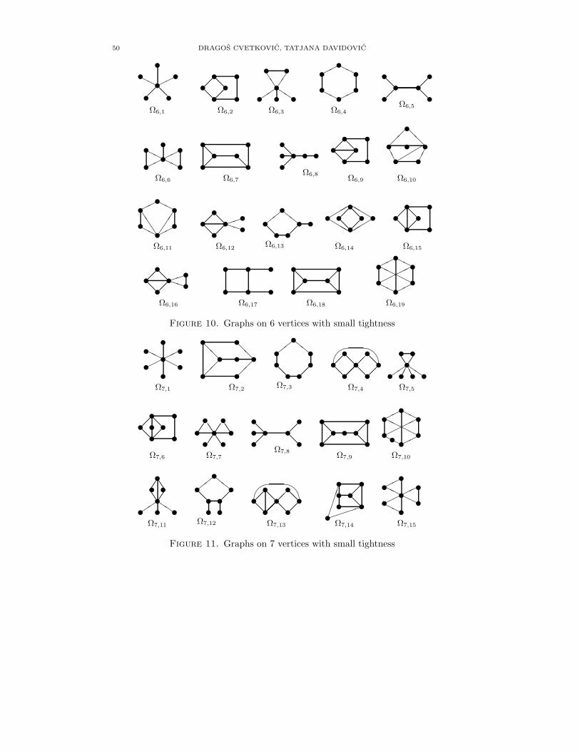
50 DRAGOS CVETKOVIC, TATJANA DAVIDOVIC
� �
� �
�
�
���� ��
Ω6,1
� �
� �
� �
��������
Ω6,2
� � �
�
� �
�� ������
Ω6,3
�
�
� �
� �
��
��
Ω6,4
�
�
� �
�
�
����
����
Ω6,5
�
�
��
�
�
��
��
Ω6,6
� �
� �
� ����� ��
Ω6,7
�
�
�
� � �����
Ω6,8
� �
� �
� �
��������
Ω6,9
�
�
� �
� �
��
����
���
Ω6,10
�
�
� �
� �
��
��
���
���
Ω6,11
�
�
� ��
�
������������
Ω6,12
� �
� �
�
�
�� ������
Ω6,13
�
� � �
�
�
����
������
����������
Ω6,14
� �
� �
� �
��������
Ω6,15
�
�
� ��
�
������������
Ω6,16
�
�
�
�
�
�
Ω6,17
� �
� �
� ����� ��
��
Ω6,18
�
�
� �
� �
��
��
����
Ω6,19
Figure 10. Graphs on 6 vertices with small tightness
�
�
� �
� �
�
����
Ω7,1
�
�
� �
�
�
�
��
��
��
��
Ω7,2
� �
� �
�
� �
����
�� ��Ω7,3
� �
� � �
� �
�����
��������
������
�
Ω7,4
� � � �
�
� �
�� �� ������
Ω7,5
� �
� � �
� �
��������
Ω7,6
� �
�� �
� �
�� ����������
Ω7,7
�
�
�
� �
�
�
����
����
Ω7,8
� �
� �
� � ����� ��
��
Ω7,9
�
�
� �
� �
� ��
��
����
Ω7,10
� � �
�
� �
�
�� ����������
Ω7,11
� �
� �
�
� �
�� ������
Ω7,12
� �
� � �
� �
�����
��������
������
�
Ω7,13
�
�
�
�
�
�
�
����
����
����
Ω7,14
�
�
� �
� �
�
��
����
Ω7,15
Figure 11. Graphs on 7 vertices with small tightness

MULTIPROCESSOR INTERCONNECTION NETWORKS 51
� �
� �
�
� �
�
����
�� ���� ��
Ω8,1
� � � �
�
� �
��� �� ������
Ω8,2
�
��
�
� �
� ���������
������
��
���
���
Ω8,3
� �
� � ��
� �
�����
��������
������
�
Ω8,4
� ��
�� �
� �
��
��
��
����
Ω8,5
�
� �
� �
� �
�
������
��
����
�� ��
Ω8,6
�
� �
� �
� �
�
����
����
����
�� ��
Ω8,7
Figure 12. Graphs on 8 vertices with small tightness
�
� �
� �
� �
�
�
����
����
Ω9,1
� � � � � �
�
� �
������
������
������������
Ω9,2
� �
� �
�
� �
�
� �
����
�� ���� ���� ��
Ω10,1
� �
� �
�
���
���
���
� �
� �
�
���
���
���
�� ��
!!
Ω10,2
Figure 13. Graphs on 9 and 10 vertices with small tightness
The main result of [5] is the next theorem. In [5] only a sketch of a proof isgiven. The proof is completed in [9].
Theorem 2. The only non-trivial connected graphs G such that t2(G) � 9 are the69 graphs Ωn,k, depicted on Figs. 8–13.
Proof of Theorem 2. We have the following cases:
a◦: D = 1, λ1 � 4.5. We have complete graphs Ω2,1, Ω3,1, Ω4,3, Ω5,8.b◦: D = 2, λ1 � 3. Denote the set of graphs satisfying these conditions by
A1. According to (2) from the introductory chapter we have Δ � λ21 � 9and by formula (3) we get n � 1 + 9 + 9 · 8 = 82. For example, the starΩ10,1 ∈ A1. The set A1 is completely determined in Lemma 2.
c◦: D = 3, λ1 � 2.25. Denote the set of graphs satisfying these conditions byA2. Now, Δ � 5 since λ21 < 6, and we have n � 1 + 5+ 5 · 4 + 5 · 42 = 106.Graphs belonging to the set A2 are listed in Lemma 3.
d◦: D = 4, λ1 � 1.8. It is easy to see that the only graph in this case is thepath Ω5,12 (see information on Smith graphs in Section 2 of the introductorychapter).
e◦: D � 5, λ1 � 1.5. There are no graphs satisfying these conditions.
To treat the cases b◦ and c◦ in Lemmas 2 and 3 we need an auxiliary result.Let R be the set of graphs satisfying the conditions D = 2, Δ = 3.

52 DRAGOS CVETKOVIC, TATJANA DAVIDOVIC
Lemma 1. The set R consists of the following 17 graphs: Ω4,1, Ω4,5, Ω4,6, Ω5,4,Ω5,6, Ω5,11, Ω6,2, Ω6,7, Ω6,9, Ω6,18, Ω6,19, Ω7,2, Ω7,9, Ω7,10, Ω8,6, Ω8,7 and Ω10,2.
Proof. By formula (3) graphs from R have at most 10 vertices. Consider a graphG ∈ R. It has a vertex v of degree 3. Let f be the number of edges in the subgraphof G induced by the three neighbours of v. We have the following possibilities:
If f = 3, we have G = Ω4,3 which is excluded since D = 1.Consider f = 2. Now we start from vertex v and its neighbours and add new
vertices and edges in such a way that conditions D = 2, Δ = 3 are not violated.We readily get G = Ω4,6, or G = Ω5,11 given on Fig. 9, or G is isomorphic to Ω6,9
from Fig. 10.In the case f = 1 the obtained graphs up to 7 vertices are presented on Fig. 14.
Finally, we get the graph Ω8,6 from Fig. 12 on n = 8 vertices.
�
�
�
�
���
���
Ω4,5
�
�
�
�
����
���
����
Ω5,6
�
�
�
�
���
��
���
���� ����
����
Ω6,7
�
�
�
�
���
��
���
���� """ ����
����
Ω6,18
�
�
�
�
�
�
�
���
���
��
Ω7,2
�
�
�
�
�
�
�
���
���
��
��
Ω7,9
Figure 14. Some graphs from the set R
If f = 0, we first have complete bipartite graphs Ω4,1, Ω5,4, and Ω6,19, and Ω6,2.For n = 7 we again come across graph Ω7,2, and the graph Ω7,10. For n = 8 thegraphs Ω8,6, Ω8,7 from Fig. 12 appear. The Petersen graph Ω10,2 on 10 verticesbelongs here. There are no graphs on 9 vertices. �
Lemma 2. The set A1 consists of 52 graphs given below.
n = 3 : Ω3,2;
n = 4 : Ω4,1, Ω4,2, Ω4,6, Ω4,5;
n = 5 : Ω5,1, Ω5,2, Ω5,3, Ω5,4, Ω5,6, Ω5,7, Ω5,9, Ω5,11, Ω5,13, Ω5,15;
n = 6 : Ω6,1, Ω6,2, Ω6,3, Ω6,6, Ω6,7, Ω6,9, Ω6,10, Ω6,11, Ω6,12, Ω6,14,
Ω6,15, Ω6,16, Ω6,18, Ω6,19;
n = 7 : Ω7,1, Ω7,2, Ω7,4, Ω7,5, Ω7,6, Ω7,7, Ω7,9, Ω7,10, Ω7,11, Ω7,13;
Ω7,14, Ω7,15;
n = 8 : Ω8,1, Ω8,2, Ω8,3, Ω8,4, Ω8,5, Ω8,6, Ω8,7;
n = 9 : Ω9,1, Ω9,2;
n = 10 : Ω10,1, Ω10,2 (the Petersen graph).
Proof. We shall first prove that there are no graphs on n > 10 vertices with diameter2 and index less than or equal to 3.
MULTIPROCESSOR INTERCONNECTION NETWORKS 53
Assume to the contrary that G is a graph on n > 10 vertices such that diam(G) =2 and λ1(G) � 3.
We first claim that Δ(G) � 8. Otherwise, if Δ(G) � 9 then λ1(G) > λ1(SΔ+1) =√Δ � 3, a contradiction. If δ(G) = 1, let v be a pendant vertex G, and w its
neighbour. Since the eccentricity of v is at most 2, w must be adjacent to allvertices of G, but then n � 10, a contradiction.
Therefore, we can assume further on that δ(G) > 1 and Δ(G) < 9. Let e be thenumber of edges of G. Then,
3 � λ1(G) �2e
n= d
and the average vertex degree is less than or equal to 3, with equality if and onlyif G is regular. If G is 3-regular graph with diameter 2, by (4) G can have at most1 + 3 + 3 · 2 = 10 vertices, a contradiction.
So the average vertex degree of G is less than 3, and since none of them is ofdegree 1, nor all are of degree 3, there exists at least one vertex in G, say u, ofdegree 2. Denote with v and w its neighbours. Let the remaining vertices (n − 3in total) be partitioned as follows: A contains the vertices that are adjacent onlyto v; B contains the vertices that are adjacent only to w; C contains the verticesthat are adjacent to both, v and w. If so
|A|+ |C| � 7 and |B|+ |C| � 7.
Since |A|+ |B|+ |C| = n− 3 and n > 10, we have |A| > 0 and |B| > 0.
Let all edges incident to v or w be coloured in blue, while the other edges, non-incident to v or w (incident only to vertices from A ∪ B ∪ C) be coloured in red.Let eb and er be the number of blue and red edges in G, respectively. Clearly,eb � n− 1 + |C|.
We now claim that er � |A| + |B| − 1. To see this, assume first that H =〈A ∪ B ∪ C〉 (the subgraph induced by the vertex set A ∪ B ∪ C) is connected.Then, er � |A|+ |B|+ |C| − 1 � |A|+ |B| − 1 and we are done. Let x and y be thevertices belonging to different components of H . Since G is of diameter 2, there isa vertex z adjacent to both vertices x and y. Clearly, z = u (otherwise, if z = uthen x = v and y = w, a contradiction). If z ∈ A ∪B ∪C, then x and y are not indifferent components of H . So z = v or z = w. If z = v then x, y ∈ A ∪C; while ifz = w then x, y ∈ B ∪ C. It follows that all vertices from the sets A and B are inthe same component of H (since x and y cannot belong to A ∪ B), and thereforeer � |A|+ |B| − 1, as required.
Consequently, we have
3n
2� e = eb + er � (n− 1 + |C|) + (|A|+ |B| − 1) = 2n− 5.
But this is equivalent to n � 10, a contradiction.Hence, there are no graphs on n > 10 vertices with diameter 2 and index less
than or equal to 3.

54 DRAGOS CVETKOVIC, TATJANA DAVIDOVIC
By an exhaustive search of connected graphs up to ten vertices one can verify thatonly the 52 graphs, quoted in the statement of the lemma fulfill the requirements.
�
Remark 1. (i) The exhaustive search in [5] was performed by the program nauty.We used publicly available library of programs nauty [29] to generate all con-
nected graphs with up to 10 vertices. nauty is a program for computing auto-morphism groups of graphs and digraphs. It can also produce a canonical graphlabelling. nauty is an open source available function library written in a portablesubset of C, and runs on a considerable number of different systems. We usedits functions for generating all connected graphs on a given number of vertices.The implemented algorithm for generation of graphs is very efficient and providesa compact representation which is not readable by ordinary users. nauty libraryalso provides several functions for converting this compact representation into “userfriendly” form.
(ii) Another possibility to find the 52 graphs from Lemma 2 is to use computerassisted reasoning.
Graphs up to 7 vertices can be found using existing graph tables [15, 16] (up to6 vertices), [13] (7 vertices).
Using an interactive graph package we follow the effect of adding vertices andedges to the largest eigenvalue λ1. (We have used the package newGRAPH availableat the address http://www.mi.sanu.ac.rs/newgraph/.)
If Δ = k, then there exists a subgraph in the form of the star Sk+1.If Δ = 9, the only solution is Ω10,1 = S10, in all other cases λ1 > 3.If Δ = 8, only one edge can be added and we get Ω9,1 = S9 and Ω9,2. Adding a
vertex yields λ1 > 3.If Δ = 7, at most two edges can be added and we get Ω8,1 = S8, Ω8,2 and Ω8,5.If Δ = 6, addition of at most three edges is possible and we get Ω7,1 = S7, Ω7,5,
Ω7,7, Ω7,11, Ω7,15.If Δ = 5, again by adding at most three edges we get Ω6,1 = S6, Ω6,3, Ω6,6,
Ω6,12, Ω6,15. Now adding vertices in a specific way is possible and we get Ω8,4.If Δ = 4, we get Ω8,3 and graphs with less than 8 vertices can be found by graph
tables.The case Δ = 3 is covered by Lemma 1, while the cases Δ < 3 are trivial.
Lemma 3. The set A2 consists of 12 graphs listed below.
n = 4 : Ω4,4; n = 5 : Ω5,5, Ω5,10, Ω5,14;
n = 6 : Ω6,4, Ω6,5, Ω6,8, Ω6,13, Ω6,17; n = 7 : Ω7,3, Ω7,8, Ω7,12.
Proof. By Table 3 given in Appendix the above 12 graphs clearly belong to the setA2. We shall show that no other graphs H belong to A2.
Maximal degree of H cannot be at least 5 since in this case H would contain S6
with an additional vertex (since D = 3). Such a subgraph would have λ1 > 2.25which is forbidden.
If Δ = 4, H contains a subgraph isomorphic to S5. We cannot add an edge toS5, since then we obtain Ω5,3 with λ1 > 2.25 (see Table 3). However, S5 can be

MULTIPROCESSOR INTERCONNECTION NETWORKS 55
extended with new vertices to graphs Ω6,8 and Ω7,8. No other extensions of verticesand edges are feasible.
Next we have to consider the case Δ � 3. Now formula (3) gives that H canhave at most 10 vertices which completes the proof using Lemma 1. �
This completes the proof of Theorem 2.
Let Gc be the set of connected graphs with at least two vertices. Let us introducethe following notation:
T a1 = {G : G ∈ Gc, t1(G) � a}, T a
stt = {G : G ∈ Gc, stt(G) � a},T aspt = {G : G ∈ Gc, spt(G) � a}, T a
2 = {G : G ∈ Gc, t2(G) � a}.It is obvious that T a
1 ⊆ T astt ⊆ T a
2 and T a1 ⊆ T a
spt ⊆ T a2 because of the partial order
between tightness values given on Fig. 2.Using Table 3 from Appendix we can immediately verify the following corollaries
of Theorem 2.
Corollary 3. The only non-trivial connected graphs G such that t1(G) � 9 are 14graphs Ωi,j, where (i, j) is:
(2, 1), (3, 1), (3, 2), (4, j) (j ∈ {1, . . . , 4}),(5, j) (j ∈ {2, 4, 8}), (6, 4), (6, 19), (7, 3), (10, 2).
Corollary 4. The only non-trivial connected graphs G such that stt(G) � 9 are 27graphs Ωi,j, where (i, j) is:
(2, 1), (3, 1), (3, 2), (4, j) (j ∈ {1, . . . , 6}), (5, j) (j ∈ {2, 4, 6, 8, 11},(6, j) (j ∈ {2, 4, 7, 9, 18, 19}), (7, j) (j ∈ {2, 3, 9, 10}), (8, 6), (8, 7), (10, 2).
Corollary 5. The only non-trivial connected graphs G such that spt(G) � 9 are21 graphs Ωi,j, where (i, j) is:
(2, 1), (3, 1), (3, 2), (4, j) (j ∈ {1, . . . , 5}), (5, j) (j ∈ {1, 2, 4, 8, }),(6, j) (j ∈ {1, 4, 14, 19}), (7, 1), (7, 3), (8, 1), (10, 2).
Corollaries 1–3 have been proved in [5] in another way.
Remark 2. In fact in [5] we have proved that T 92 = Q∪R′∪S′∪V ′, where T 9
1 = Q,T 9stt = Q ∪R′, T 9
spt = Q ∪ S′ and |T 92 | = 69.
Here we have
Q = {K2,K3,K4,K5, P3, P4, C4, C5, C6, C7,K1,3,K2,3,K3,3, PG},S′ = {P5,K1,4,K1,5,K1,6,K1,7,K1,8,K1,9},R′ = {Ω4,5,Ω4,6,Ω5,6,Ω5,11,Ω6,2,Ω6,7,Ω6,9,Ω6,18,Ω7,2,Ω7,9,Ω7,10,Ω8,6,Ω8,7}
and V ′ consists of the remaining 35 graphs. Here, PG denotes the Petersen graph.We see that the sets Q and S′ (related to tightness t1 and spt) contain only thestandard graphs. When considering stt and t2, the graphs with non-standard namesoccur.

56 DRAGOS CVETKOVIC, TATJANA DAVIDOVIC
7. Graphs with smallest tightness values
One of the goals in this work is to identify graphs with smallest tightness valuesfor all four types of tightness.
Based on Corollary 1 of Theorem 2 we are in a position to find the best config-urations w.r.t. t1 up to 10 vertices.
Theorem 3. Among connected graphs G on n (n � 10) vertices the value t1(G) isminimal for the following graphs:
K2 for n = 2, C5 for n = 5, C8 for n = 8,
K3 for n = 3, C6 for n = 6, C9 for n = 9,
K4 for n = 4, C7 for n = 7, the Petersen graph for n = 10.
Proof. By Theorem 2, all connected graphs G with t1(G) at most 9 are known.Among them it is easy to identify graphs with minimal tightness for n � 7 andn = 10. The cases n = 8, 9 remain. Since m and Δ are both integers, the nextunexamined value for t1 is ten. We easily find that for C8 and C9, having m = 5and Δ = 2, tightness value t1 = 10. �
In a similar way we can identify extremal graphs for other types of tightnessbased on the results presented in the previous section. The obtained graphs aresummarized in Table 2. Together with extremal graphs, the corresponding tightnessvalues are given in parentheses.
Table 2. Minimal graphs with their tightness values
n t1 stt spt t22 K2 (2) K2 (2) K2 (2) K2 (2)3 K3 (4) K3 (4) K3 (4) K3 (4)4 K4, C4 (6) K4, C4 (6) S4 (5.196) S4 (5.196)5 C5 (6) C5 (6) C5, S5 (6) C5, S5 (6)6 C6 (8) C6 (8) S6 (6.708)) S6 (6.708))7 C7 (8) C7 (8) S7 (7.348) S7 (7.348)8 C8 (10) N(8, 6660), N(8, 8469) (9) S8 (7.937) S8 (7.937)9 C9 (10) C9 (10) S9 (8.485) S9 (8.485)10 PG (9) PG (9) PG, S10 (9) PG, S10 (9)
Several interesting observations can be made.For n = 2 and n = 3 complete graphs (in a trivial way) are minimal graphs
for all four types of tightness. Starting from n = 4, tightness spt and t2 start tosuggest stars as best interconnection networks while tightness t1 and stt start tosuggest circuits as the best ones. Surprises come for n = 8 and n = 10.
For n = 8 according to the tightness stt we get two cubic graphs N(8, 6660) andN(8, 8469) (graphs in which all vertex degrees are equal to 3) of diameter 2. Thesegraphs break the circuit sequence of minimal graphs for stt. They also representthe only case (among small graphs) when t1 and stt have different minimal values.
MULTIPROCESSOR INTERCONNECTION NETWORKS 57
For n = 10 the Petersen graph (PG) appears in all four cases. It is also a cubicgraph of diameter 2. In addition, it is strongly regular, which means that anytwo adjacent vertices have a fixed number (0 in this case) of common neighborsand any two non-adjacent vertices have a fixed number (1 in this case) of commonneighbors. Such an extraordinary structure is the reason why the Petersen graphappears frequently in graph theory as example or counterexample in numerousstudies. Here it appears that the Petersen graph should be considered as a verygood multiprocessor interconnection network. It is also remarkable that tightnesst1 and stt cannot be smaller than 10 for n = 9 and that only with one vertex more,when n = 10 their value can become 9 for the Petersen graph.
However, by tightness spt and t2, the star on 10 vertices is as equally goodtopology as the Petersen graph.
The results for spt and t2 perhaps suggest that stars are candidates for optimaltopologies in general. However, such a conclusion is correct only for small graphs.In [6] it was shown that stars have tightness spt and t2 asymptotically equal toO(
√n) while hypercubes have equal values for all four types of tightness with
asymptotical behavior O((log n)2). On the other hand, 3-dimensional hypercubeseems to be less suitable not only than the star S8; N(8, 6660), N(8, 8469), C8 andsome other graphs also have smaller tightness values. Moreover, graphs N(8, 6660)and N(8, 8469) provide a smaller diameter with the same maximum vertex degree.
The problem of finding graphs with the smallest tightness values for a givennumber of vertices remains open in general.
References
[1] U. Borstnik, M. Hodoscek, and D. Janezic, Fast parallel molecular simulations, Croat. Chem.Acta, 78(2):211–216, 2005.
[2] V. Brankov, D. Cvetkovic, S. Simic, and D. Stevanovic, Simultaneous editing and multil-abelling of graphs in system newGRAPH, Univ. Beograd, Publ. Elektrotehn. Fak. Ser. Mat.
17:112–121, 2006.[3] A. E. Brouwer, A. M. Cohen, and A. Neumaier, Distance-regular Graphs, Springer, Berlin,
1989.[4] G. T. Byrd and B. A. Delagi, Considerations for multiprocessor topologies, Technical report,
STAN-CS-87-1144, Department of Computer Science, Stanford University, 1987.[5] D. Cvetkovic and T. Davidovic, Multiprocessor interconnection networks with small tightness,
Internat. J. Foundations Computer Sci., 20(5):941–963, 2009.[6] D. Cvetkovic and T. Davidovic, Application of some graph invariants to the analysis of
multiprocessor interconnection networks, Yugosl. J. Oper. Res. 18(2):173–186, 2008.[7] D. Cvetkovic and T. Davidovic, Exhaustive search for multiprocessor interconnection net-
works with small tightness value, in: D. Teodorovic, editor, Proc. SYM-OP-IS 2008, SokoBanja, Serbia, Sept. 14–17, 2008, pp. 329–332.
[8] D. Cvetkovic and T. Davidovic, Well-suited multiprocessor topologies with small number ofprocessors, Novi Sad J. Math., 38(3):209–217, 2008.
[9] D. Cvetkovic, T. Davidovic, A. Ilic, S.K. Simic, Graphs for small multiprocessor intercon-nection networks, Appl. Math. Computation 217:2468–2480, 2010.
[10] D. Cvetkovic, V. Dimitrijevic, and M. Milosavljevic, A survey of some non-standard travelingsalesman problems, Yugosl. J. Oper. Res. 2(2):163–185, 1992.
[11] D. Cvetkovic and I. Gutman, Note on branching, Croat. Chem. Acta 49:115–121, 1977.[12] D. Cvetkovic and P. Rowlinson, The largest eigenvalue of a graph – a survey, Linear Multi-
linear Algebra 28:3–33, 1990.

58 DRAGOS CVETKOVIC, TATJANA DAVIDOVIC
[13] D. M. Cvetkovic, M. Doob, I. Gutman, and A. Torgasev, Recent Results in the Theory ofGraph Spectra, North Holland, Amsterdam, 1988.
[14] D. M. Cvetkovic, M. Doob, and H. Sachs, Spectra of Graphs: Theory and Applications, (IIIedition), Johann Ambrosius Barth Verlag, Heidelberg–Leipzig, 1995.
[15] D. M. Cvetkovic and M. Petric, A table of connected graphs on six vertices, Discrete Math.50:37–49, 1984.
[16] D. Cvetkovic, P.‘Rowlinson, S. Simic, An Introduction to the Theory of Graph Spectra, Cam-bridge University Press, Cambridge, 2009.
[17] T. Decker, B. Monien, and R. Preis, Towards optimal load balancing topologies, in Proc. 6thEuroPar Conf., Lect. Notes Comput. Sci. 1900, Springer, Berlin, p.p. 277–287
[18] R. Dickmann, A. Frommer, and B. Monien, Efficient scheme for nearest neighbor load bal-ancing, Parallel Comput. 25:789–812, 1999.
[19] R. Elsasser, R. Kralovic, and B. Monien, Sparse topologies with small spectrum size, Theor.Comput. Sci. 307:549–565, 2003.
[20] A. Ferreira and M. Morvan, Models for parallel algorithm design: An introduction, in:A. Migdalas, P. Pardalos, and S. Storøy, editors, Parallel Computing in Optimization,Kluwer, Dordrecht/Boston/London, 1997, p.p. 1–26.
[21] P. W. Fowler, G. Caporossi, and P. Hansen, Distance matrices, Wiener indices, and relatedinvariants of fullerenes, J. Chem. Phys. A 105:6232–6242, 2001.
[22] P. W. Fowler and D. E. Manolopoulos, An Atlas of Fullerenes, Clarendon Press, Oxford,1995.
[23] B. Ghosh, S. Muthukrishnan, and M. H. Schultz, First and second order diffusive methods forrapid, coarse, distributed load balancing, in: Proc. 8th Annual ACM Symposium on ParallelAlgorithms and Architectures (SPAA’96), ACM Press, 1996, pages 72–81,
[24] A. Gupta and P. A. Dinda, Inferring the topology and traffic load of parallel programs runningin a virtual machine environment, Lect. Notes Comput. Sci. 3277:125–143, 2005.
[25] I. Gutman, Characteristic and matching polynomials of some compound graphs, Publ. Inst.Math., Nouv. Ser. 27(41):61–66, 1980.
[26] Y. F. Hu and R. J. Blake, An improved diffusion algorithm for dymanic load balancing,Parallel Comput. 25:417–444, 1999.
[27] Y. F. Hu, R. J. Blake, and D. R. Emerson, An optimal migration algorithm for dymanic loadbalancing, Concurrency Pract. Exp. 10:467–483, 1998.
[28] F. T. Leighton, Introduction to Parallel Algorithms and Architectures, Arrays, Trees, Hy-percubes, Morgan Kaufmann, San Mateo, 1992.
[29] B. D. McKay, Nauty user’s guide (version 2.2), Technical report, http://cs.anu.edu.au-/˜bdm/nauty, 2006.
[30] K. Qiu and S. K. Das, Interconnection networks and their eigenvalues, Int. J. Found. Comput.Sci. 14(3):371–389, 2003.
[31] V. Sarkar, Partitioning and Scheduling Parallel Programs for Multiprocessors, M.I.T. Press,Cambridge, MA, 1989.
[32] M. Sevkli and M. E. Aydin, Parallel variable neighbourhood search algorithms for job shopscheduling problems, IMA J. Math. Manage. 18(2):117–133, April 2007.
[33] G. C. Sih and E. A. Lee, A compile-time scheduling heuristic for interconnection-constrainedheterogeneous processor architectures, IEEE Trans. Paral. Dist. Syst. 4(2):175–187, February1993.
[34] S. Simic and D. Tosic, The index of trees with specified maximum degree, MATCH Commun.Math. Comput. Chem 54:351–362, 2005.
[35] T. Sørevik, A programmer’s view of parallel computers, in: A. Migdalas, P. Pardalos, andS. Storøy, editors, Parallel Computing in Optimization, Kluwer, Dordrecht/Boston/London,1997, p.p. 57–72.
[36] E. van Dam, Graphs with few eigenvalues, An interplay between combinatorics and algebra,PhD thesis, Center for Economic Research, Tilburg University, 1996.

MULTIPROCESSOR INTERCONNECTION NETWORKS 59
[37] L. Wang, Z. P. Chen, and X. H. Jiang, Ringed Petersen spheres connected hypercube intercon-nection networks, in: Proc. 10th IEEE Int. Conf. Eng. Complex Comput. Sys. (ICECCS’05),IEEE Computer Society, 2005, p.p. 127–131,
Appendix
The Table 3 given below contains some relevant data about 69 graphs withsecond type mixed tightness not exceeding 9.
Graphs are ordered first by n (the number of vertices), and within the groupswith fixed n, by t2. Columns of the table provide graph name, the number ofvertices n, the number of edges e, the name(s) under which the graph appeared in[5], diameter D, maximum vertex degree Δ, the number of distinct eigenvalues m,the spectrum starting with the largest eigenvalue λ1. Last four columns containthe values of the four types of tightness t1, stt, spt, t2.
As “the old names” we used different notation. First we distinguish the wellknown graphs such as complete graphs, circuits, stars, complete bipartite graphs,and so on. For graphs up to 5 vertices we used the notation from [14], while graphson n = 6 vertices are marked primarily as in [15]. N(n, j) denotes the j-th graphon n vertices generated by program nauty. PG denotes the well known Petersengraph.

60
Table3.Graphsonupto
10verticeswithsm
alltightness
graph
ne
old
name(s)
DΔ
mλ1,λ
2,...,λ
nt 1
stt
spt
t 2Ω
2,1
21
G1=
K2=
P2
11
21,-1
22
22
Ω3,1
33
G2=
K3=
C3
12
22,-1,-1
44
44
Ω3,2
2G
3=
P3=
S3=
K1,2
22
31.41,0,-1.41
66
4.23
4.23
Ω4,1
43
G8=
S4=
K1,3
23
31.73,0,0,-1.73
99
5.19
5.19
Ω4,2
4G
7=
C4=
K2,2
22
32,0,0,-2
66
66
Ω4,3
6G
4=
K4
13
23,-1,-1,-1
66
66
Ω4,4
3G
9=
P4
32
41.62,1.62,0.62,-0.62,-1.62
88
6.47
6.47
Ω4,5
4G
62
34
2.17,0.31,-1,-1.48
12
98.68
6.51
Ω4,6
5G
52
34
2.56,0,-1,-1.56
12
910.24
7.68
Ω5,1
55
G28=
S5=
K1,4
24
32,0,0,0,-2
12
12
66
Ω5,2
5G
27=
C5
22
32,0.62,0.62,-1.62,-1.62
66
66
Ω5,3
5G
23
24
52.34,0.47,0,-1,-1.81
20
12
11.71
7.03
Ω5,4
6G
22=
K2,3
23
32.45,0,0,0,-2.45
99
7.35
7.35
Ω5,5
4G
29
33
51.85,0.77,0,-0.77,-1.85
15
12
9.24
7.39
Ω5,6
6G
21
23
52.48,0.69,0,-1.17,-2
15
912.41
7.44
Ω5,7
6G
20
24
42.56,1,-1,-1,-1.46
16
12
10.25
7.68
Ω5,8
10
G10=
K5
14
24,-1,-1,-1,-1
88
88
Ω5,9
6G
18
24
52.69,0.33,0,-1.27,-1.75
20
12
13.43
8.06
Ω5,10
5G
26
33
52.14,0.66,0,-0.66,-2.14
15
12
10.68
8.54
Ω5,11
7G
17
23
52.86,0.32,0,-1,-2.18
15
914.28
8.57
Ω5,12
4G
30=
P5
42
51.73,1,0,-1,-1.73
10
10
8.66
8.66
Ω5,13
7G
16
24
52.94,0.62,-0.46,-1.47,-1.62
20
12
14.68
8.81
Ω5,14
5G
25
33
52.21,1,-0.54,-1,-1.67
15
12
11.07
8.86
Ω5,15
7G
15
24
43,0,0,-1,-2
16
12
12
9

61
Table
3:Graphsonupto
10verticeswithsm
alltightness(cont.)
graph
ne
old
name(s)
DΔ
mλ1,λ
2,...,λ
nt 1
stt
spt
t 2Ω
6,1
65
S6=K
1,5=CP(107)=N(6,1)
25
32.24,0,0,0,0,-2.24
15
15
6.71
6.71
Ω6,2
7CP(93)=
N(6,35)
23
62.39,0.77,0.62,0,-1.62,-2.16
18
914.35
7.17
Ω6,3
6CP(94)=
N(6,3)
25
52.51,0.57,0,0,-1,-2.09
25
15
12.57
7.54
Ω6,4
6C
6=CP(106)=N(6,49)
32
42,1,1,-1,-1,-2
88
88
Ω6,5
5CP(109)=
N(6,5)
33
52,1,0,0,-1,-2
15
12
10
8Ω
6,6
7CP(79)=
N(6,17)
25
52.71,1,0.19,-1,-1,-1.90
25
15
13.55
8.13
Ω6,7
8CP(72)=
N(6,89)
23
62.74,0.71,0.62,-0.23,-1.62,-2.22
18
916.45
8.22
Ω6,8
5CP(108)=
N(6,2)
34
52.07,0.84,0,0,-0.84,-2.07
20
16
10.37
8.30
Ω6,9
8CP(69)=
N(6,90)
23
62.79,1,0.62,-1,-1.62,-1.79
18
916.75
8.37
Ω6,10
8CP(71)=
N(6,36)
24
52.80,0.85,0,0,-1.20,-2.45
20
12
13.98
8.39
Ω6,11
8CP(68)=
N(6,57)
24
62.81,1,0.53,-1,-1.34,-2
24
12
16.88
8.44
Ω6,12
7CP(75)=
N(6,8)
25
52.81,0.53,0,0,-1.34,-2
25
15
14.07
8.44
Ω6,13
6CP(105)=
N(6,19)
33
62.11,1,0.62,-0.25,-1.62,-1.86
18
12
12.69
8.46
Ω6,14
8K
2,4=CP(73)=N(6,13)
24
32.83,0,0,0,0,-2.83
12
12
8.49
8.49
Ω6,15
8CP(66)=
N(6,39)
24
52.90,0.81,0,0,-1.71,-2
20
12
14.52
8.71
Ω6,16
8CP(61)=
N(6,32)
25
62.95,1.16,0,-1,-1.29,-1.82
30
15
17.68
8.84
Ω6,17
6CP(102)=
N(6,18)
33
62.25,0.80,0.55,-0.55,-0.80,-2.25
18
12
13.48
8.99
Ω6,18
9CP(51)=
N(6,93)
23
43,1,0,0,-2,-2
12
912
9Ω
6,19
9K
3,3
=CP(52)=
N(6,71)
23
33,0,0,0,0,-3
99
99
Ω7,1
76
S7=
K1,6
=N(7,1)
26
32.45,0,0,0,0,0,-2.45
18
18
7.35
7.35
Ω7,2
9N(7,337)
23
52.66,1.21,0.62,0.62,-1.62,-1.62,-1.87
15
913.28
7.97
Ω7,3
7C
7=
N(7,292)
32
42,1.255,1.25,-0.45,-0.45,-1.80,-1.80
88
88
Ω7,4
9N(7,156)
24
62.68,1,0.64,0,0,-2,-2.32
24
12
16.09
8.04
Ω7,5
7N(7,3)
26
52.68,0.64,0,0,0,-1,-2.32
30
18
13.41
8.04

62
Table
3:Graphsonupto
10verticeswithsm
alltightness(cont.)
graph
ne
old
name(s)
DΔ
mλ1,λ
2,...,λ
nt 1
stt
spt
t 2Ω
7,6
79
N(7,75)
24
62.75,0.84,0.62,0,0,-1.62,-2.59
24
12
16.51
8.25
Ω7,7
8N(7,23)
26
62.86,1,0.32,0,-1,-1,-2.18
36
18
17.13
8.57
Ω7,8
6N(7,5)
34
52.18,1.13,0,0,0,-1.13,-2.18
20
16
10.88
8.70
Ω7,9
10
N(7,624)
23
72.90,1.41,0.81,0,-1.41,-1.71,-2
21
920.32
8.71
Ω7,10
10
N(7,514)
23
62.90,0.81,0.73,0,0,-1.71,-2.73
18
917.42
8.71
Ω7,11
8N(7,8)
26
52.94,0.66,0,0,0,-1.37,-2.24
30
18
14.72
8.83
Ω7,12
7N(7,92)
33
62.21,1,1,0,-0.54,-1.68,-2
18
12
13.29
8.86
Ω7,13
10
N(7,448)
24
72.98,1.33,0.65,0,-1,-1.77,-2.19
28
12
20.86
8.94
Ω7,14
9N(7,324)
24
72.97,0.80,0.70,0.45,-0.55,-2.12,-2.25
28
12
20.77
8.90
Ω7,15
9N(7,219)
26
43,1,1,-1,-1,-1,-2
24
18
12
9
Ω8,1
87
S8=
K1,7
=N(8,1)
27
32.65,0,0,0,0,0,0,-2.65
21
21
7.94
7.94
Ω8,2
8N(8,3)
27
52.54,0.69,0,0,0,0,-1,-2.84
35
21
14.22
8.53
Ω8,3
11
N(8,1039)
24
82.90,1.30,0.81,0.62,0,-1.62,-1.71,-2.30
32
12
23.23
8.71
Ω8,4
11
N(8,342)
25
62.98,1.13,0.65,0,0,0,-2.07,-2.68
30
15
17.86
8.93
Ω8,5
9N(8,30)
27
63,1,0.41,0,0,-1,-1,-2.41
42
21
18
9Ω
8,6
12
N(8,8469)
23
63,1.56,0.62,0.62,0,-1.62,-1.62,-2.56
18
918
9Ω
8,7
12
N(8,6660)
23
53,1,1,0.41,0.41,-1,-2.41,-2.41
15
915
9
Ω9,1
98
S9=
K1,8
=N(9,1)
28
32.83,0,0,0,0,0,0,0,-2.83
24
24
8.49
8.49
Ω9,2
9N(9,3)
28
53,0.73,0,0,0,0,0,-1,-2.73
40
24
15
9
Ω10,1
10
9S10=
K1,9
=N(10,1)
29
33,0,0,0,0,0,0,0,0,-3
27
27
99
Ω10,2
15
PG
=N(10,8027956)
23
33,1,1,1,1,1,-2,-2,-2,-2
99
99
Silvia Gago
SPECTRAL TECHNIQUES
IN COMPLEX NETWORKS
Abstract. Most physical, biological, chemical, technological and so-cial systems have a network structure. Examples of complex networksrange from cell biology to epidemiology or to the Internet. In the re-cent years, several models of complex networks have been proposed,as the random graph of Erdos and Renyi, the small-world model ofWatts and Strogatz or the scale-free networks of Barabasi and Albert.
The topological structure of such networks can be fully describedby the associated adjacency matrices and their spectral density. Therich information about the topological structure and diffusion pro-cesses can be extracted from the spectral analysis of the networks.For instance, the power-law behavior of the density of eigenvalues isa notable feature of the spectrum of scale-free networks. Dynami-cal network processes, like synchronization can be determined by thestudy of their Laplacian eigenvalues. Furthermore, the eigenvaluesare related to many basic topological invariants of networks such asdiameter, mean distance, betweenness centrality, etc.
Spectral techniques are also used for the study of several networkproperties: community detection, bipartition, clustering, design ofhighly synchronizable networks, etc.
Mathematics Subject Classification (2010): Primary: 05-02, 05C50
Keywords : algebraic connectivity, complex networks, eigenvaluedistribution, synchronization, community structure.

Contents
1. Introduction 642. Internet graph models and their spectra 673. Synchronization 723.1. Synchronization and topological parameters. 763.2. Design of synchronizable networks 784. Community detection and spectral bisection 79References 82
1. Introduction
Complex networks are everywhere. They are formed by a large set of verticesrepresenting the entities of the system, and a set of edges, representing the interac-tions between their elements. Examples of complex networks include the Internet,World Wide Web, social networks of acquaintances or other connections betweenindividuals, distribution networks such as postal delivery routes, neural networks,food webs, metabolic networks, networks of citations between papers, organiza-tional networks and networks of business relations between companies, and manyothers (see Fig. 1). In the recent last years, two classes of complex networks havearoused a great deal of interest in the literature: small-world networks and scale-freenetworks, as many real networks exhibit characteristics of both classes.
The spectrum of the adjacency and Laplacian matrices provide a great deal ofinformation about the structure of a network. As usual, the eigenvalues of theadjacency matrix are denoted by λi, 1 � i � n. Recall that the Laplacian matrixof a graph is a symmetric matrix L whose diagonal elements lii are the degrees ofthe vertices, and whose off-diagonal elements lij are −1 if the vertex vi is connectedto vj , and 0 otherwise. More precisely, if D is the diagonal matrix of vertex degreesdi and A is the adjacency matrix of the graph, L = D − A. Note that L is semi-positive definite, xTLx � 0 for any vector x, its first eigenvector is j = (1, . . . , 1)T
corresponding to the first eigenvalue θ1 = 0, and the second largest eigenvalue θ2 iscalled the algebraic connectivity orFiedler value, because its proximity to 0 revealswhether the graph can be easily disconnected. Its corresponding eigenvector v2 isalso known as the Fiedler vector, and is essential for the bisection method. TheLaplacian spectrum is denoted by
sp(L) = {0 � θ2 � . . . � θn}.64

SPECTRAL TECHNIQUES IN COMPLEX NETWORKS 65
Figure 1. A complex network: a picture of the World Wide Web,from Hal Burch and Bill Cheswick, Lumeta Corp.
The normalized Laplacian matrix is introduced by Chung and defined as thesymmetric matrix L whose diagonal elements lii are 1, and whose off-diagonalelements lij = −1/
√didj if the vertex vi is connected to vj , and 0 otherwise. Its
relation with the Laplacian is given by L = D−1/2LD−1/2.Several topological parameters are considered for the study of complex networks.
Some of them are well known in graph theory, like the diameter, mean distance,isoperimetric number, maximum and minimum degree and edge connectivity.
The edge connectivity, e(G), of a graph G is the minimum number of edgeswhich must be deleted in G to disconnect it. The minimum and maximum degreeof the graph are denoted by δ and Δ respectively. Denoting by d(u, v) the distancebetween two vertices u, v ∈ V (G) (the length of the shortest path), the diameter isD = maxu,v∈V d(u, v), and the mean distance or average path length is
l =2
n(n− 1)
∑
(u,v)∈V (G)
d(u, v).
The graph diameter provides an inverse measure of the vertex connectivity. In-tuitively, we can say that two vertices in a network are weakly connected if their
66 SILVIA GAGO
shortest connection passes through many other vertices. When this happens for allpairs of nodes, the diameter D of the graph is large.
The isoperimetric number of a graph is introduced by Mohar in [42] as thenumber i(G) = min|X|�n
2|δX |/|X |, where X is a subset of vertices, δX is the
boundary of X , i.e., the set of edges in G between vertices in X and vertices notin X . It is a measure of whether or not a graph can be split in two subgraphsof the same cardinality. In the same paper there are two different bounds for theisoperimetric number.
New parameters and tools are also considered to characterize properties of thesenew networks, like the degree distribution, eigenvalue distribution, spectral density,clustering parameter and betweenness centrality.
Clustering parameter. Let ei be the number of edges connecting the neighbors ofa vertex ui of degree δi, then the clustering coefficient of ui is Ci = 2ei/δi(δi − 1),for any 1 � i � n, and the clustering coefficient or parameter of the graph G isdefined as
C =1
n
n∑
i=1
Ci.
Power-laws distributions. A power-law function follows the polynomial formf(x) = ax−γ , where a, γ are constants and γ is called the power-law exponent.This kind of distribution was previously known as Pareto distribution or Zipfslaw. The main property of power laws is their scale invariance, i.e., any scalingof the argument x by a constant factor causes only a proportionate scaling of thefunction itself, i.e., f(cx) = a(cx)−γ = c−γf(x) ∝ f(x), which means that they areproportional and therefore it preserves the shape of the function itself. Moreover,by taking logarithms a linear relation is obtained log f(x) = log a − γ log x. Anetwork with degree power law distribution is called scale-free.
Spectral density. Given a graph G of order n, and adjacency matrix eigenvaluesλi, 1 � i � n, the spectral density of the graph is defined as
ρ(x) =1
n
n∑
j=1
δ(x − λj), where δ(x) =
{1, if x = 0,0, if x �= 0.
is the Kronecker or delta function.Betweenness centrality. Vertex betweenness centrality was introduced by a so-
ciologist Freeman [29] in 1977, as a measure of the importance of a vertex in anetwork. Since the appearance of complex networks it has become an importantparameter to study networks features [45], generalizing the concept for edge be-tweenness centrality. Spectral bounds for either the vertex betweenness and edgebetweennes of a graph are studied in [15], and more general properties can be foundin [32]. The maximum betweenness centrality, Bmax, is also considered for studyingseveral aspects of the network, as its synchronization capability (Section 3), or usedfor performance of bisection methods (Section 4).
To be more precise, if σuv(w) denotes the number of shortest paths from ver-tex u to vertex v that go through w, and σuv is the total number of shortestpaths from u to v, then bw(u, v) = σuv(w)/σuv . The betweenness of a vertex w is

SPECTRAL TECHNIQUES IN COMPLEX NETWORKS 67
Bw =∑
u,v �=w bw(u, v). The betweenness centrality of a graph G of order n is
B =1
n
∑
u∈V
Bu,
and the maximum betweenness of the graph G is Bmax = max{Bu | u ∈ V }. Themean betweenness B is closely related with the mean distance l of the graph asB = (n − 1)(l − 1) [15]. The same parameters can be defined for edges, and themost used one is the maximum edge betweenness centrality, BE.
2. Internet graph models and their spectra
Traditionally networks have been described by either regular graphs or randommodels like the classical model of Erdos–Renyi [22]. The later consists of a graph onn vertices, G(n, p), where the vertices are connected between them with probabilityp. In particular the distribution of the degree of any particular vertex v is binomial
P (dv = k) =
(n
k
)pk(1− p)n−k.
Figure 2. Watts and Strogatz small-world model. The diagramrepresents the rewiring probability p versus normalized mean dis-tance l and clustering parameter C. Observe that as p increases,both l and C decrease. However, l decays faster than C, whichallows a probability region, 0.01 � p � 0.1, where l is a small andC is still high.
However, the appearance of new networks like the Internet graph, which couldnot be reproduced by these classical models, motivated Watts and Strogatz to intro-duce a new model for describing them [60]. They observed that such networks havea small diameter or mean distance as the former, and a large clustering parameter,as the later. Sparse random graphs have a small clustering coefficient while realworld networks often have a coefficient significantly larger.

68 SILVIA GAGO
The model proposed by Watts and Strogatz starts from a regular graph with alarge clustering parameter, which is transformed into a small world graph by therandom reconnection of only a small number of edges, as the diameter is drasticallyreduced while the clustering coefficient of the regular graph remains large (seeFig. 2).
Since the appearance of this breakthrough a large number of stochastic anddeterministic models have been appearing in the literature. For more informationabout them we refer the reader to the surveys [6] and [14].
In 1999 Faloutsos, Faloutsos and Faloutsos [25] made an experimental study ofone part of the Internet graph, obtaining power laws in the distribution of manyof the different parameters of the network, as the vertex degrees or the adjacencymatrix eigenvalues. A typical value for the degree power-law exponent in realnetworks is 2 � γ � 3. For obtaining the eigenvalue power-law, the eigenvaluesλi of the adjacency matrix are sorted in decreasing order and plotted versus theassociated increasing sequence of numbers i representing the order of the eigenvalue(see Fig. 3). A similar relation has been recently obtained for the normalizedLaplacian eigenvalues in [53] and for the weighted Laplacian and the weightedadjacency matrix in [38]. Former experimental studies indicate that the powerlaw exponents have not changed over the years in spite of the exponential networkgrowth [34, 52].
Figure 3. Power law distributions at the AS level Oregon Internetnetwork, from [25]. On the left it is represented the histogramof 10000 highest vertex degrees and on the right the 100 largesteigenvalues versus their order, both in a log-log scale.
Mihail et al. in [41] found a surprising relationship between the degree and theeigenvalue exponents: the eigenvalue exponent is approximately half of the degreeexponent. This fact indicates that the first largest eigenvalues are the square rootof the first largest degrees. They also claimed that the eigenvalue distributionis a consequence of the degree distribution. However, in [31] it is proved by theconstruction of a deterministic model based on direct products of star graphs thatthe eigenvalue power-law is not a consequence of the degree power-law.
SPECTRAL TECHNIQUES IN COMPLEX NETWORKS 69
Among the scale-free models the most studied one is proposed by Barabasi andAlbert in 1999 [2]. The model is based on two observed facts in real networks:networks expand continuously by the addition of new vertices, and new verticesattach preferentially to sites that are already well connected. They used the so-called preferential attachment model. The model starts with a small number ofvertices m0 at step t = 0, and at every time step a new vertex u is connected tom � m0 vertices of the existing graph. The probability of the new vertex u of beingconnected to an existing vertex ui depends on its degree di, i.e.,
p(u is connected to ui) = pi =di∑j dj
, for 1 � i � m.
The Barabasi–Albert model produces a degree power-law distribution with expo-nent γ = −3, meanwhile the Watts and Strogatz and the Erdos-Renyi follow aPoisson distribution. This means that vertices with higher degree have strongerability to grab links added to the network.
The main tool used for studying the spectra of large complex networks is thespectral density ρ(λ). For a uncorrelated random graph, a graph where the prob-ability for any pair of its vertices being connected is the same, p, and where theseprobabilities are independent variables, the adjacency matrix A is a real symmet-ric n × n uncorrelated random matrix, i.e., EAij = 0 and EA2
ij = σ. For thismatrix, the limit of the spectral density when n → ∞ converges to a semicirculardistribution (if rescaled as λ′ = λ[np(1− p)]−1/2 ∝ λn−1/2)
ρ(λ′) ={
(2π)−1√4− λ′2, if |λ′| < 2σ,
0, otherwhise.
This theorem is known as Wigner’s semicircular law [61]. Surprisingly, the semi-circular spectral density is not valid for any realistic graph models.
The spectrum and the corresponding eigenvectors of the Barabasi and Albertmodel have been studied by Goh et al. in [35] obtaining that the distribution ofthe spectra is quite far from a semicircle. The eigenvalues decay exponentiallyaround the center and have power-law long tails at both edges. The same resultwas obtained by Farkas et al. in [26], where the spectral density of both Wattsand Strogatz and Barabasi and Albert models are studied, finding that they havea special shape. In particular, scale-free graphs develop a triangle-like spectraldensity with a power-law tail when plotted in log-log scale (see Fig. 4), while small-world graphs have a complex spectral density consisting of several sharp peaks(Fig. 5). They also found that the eigenvalues λ1 and |λn| depend on n as n1/4
for large n, and that the eigenvector corresponding to the largest eigenvalue isstrongly localized at the vertex with the largest degree and is independent of thesystem size n.
Nevertheless, Chung et al. [11] showed that, depending on the matrix, under acertain mild condition (that the minimum expected degree is significantly largerthan the square root of the expected average degree), the eigenvalues of the nor-malized Laplacian of a random power-law graph follow the semicircle law, whereasthe spectrum of the adjacency matrix of a power-law graph obeys the power law.
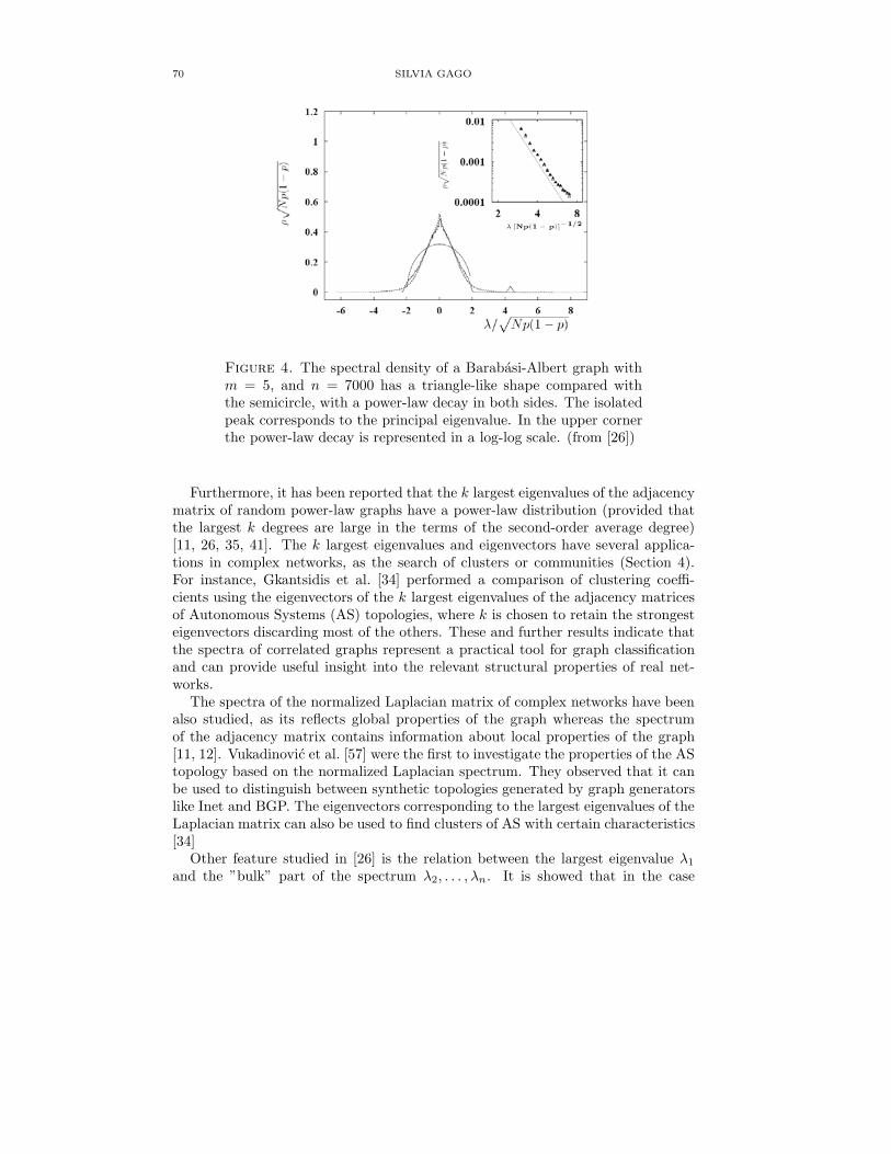
70 SILVIA GAGO
Figure 4. The spectral density of a Barabasi-Albert graph withm = 5, and n = 7000 has a triangle-like shape compared withthe semicircle, with a power-law decay in both sides. The isolatedpeak corresponds to the principal eigenvalue. In the upper cornerthe power-law decay is represented in a log-log scale. (from [26])
Furthermore, it has been reported that the k largest eigenvalues of the adjacencymatrix of random power-law graphs have a power-law distribution (provided thatthe largest k degrees are large in the terms of the second-order average degree)[11, 26, 35, 41]. The k largest eigenvalues and eigenvectors have several applica-tions in complex networks, as the search of clusters or communities (Section 4).For instance, Gkantsidis et al. [34] performed a comparison of clustering coeffi-cients using the eigenvectors of the k largest eigenvalues of the adjacency matricesof Autonomous Systems (AS) topologies, where k is chosen to retain the strongesteigenvectors discarding most of the others. These and further results indicate thatthe spectra of correlated graphs represent a practical tool for graph classificationand can provide useful insight into the relevant structural properties of real net-works.
The spectra of the normalized Laplacian matrix of complex networks have beenalso studied, as its reflects global properties of the graph whereas the spectrumof the adjacency matrix contains information about local properties of the graph[11, 12]. Vukadinovic et al. [57] were the first to investigate the properties of the AStopology based on the normalized Laplacian spectrum. They observed that it canbe used to distinguish between synthetic topologies generated by graph generatorslike Inet and BGP. The eigenvectors corresponding to the largest eigenvalues of theLaplacian matrix can also be used to find clusters of AS with certain characteristics[34]
Other feature studied in [26] is the relation between the largest eigenvalue λ1and the ”bulk” part of the spectrum λ2, . . . , λn. It is showed that in the case
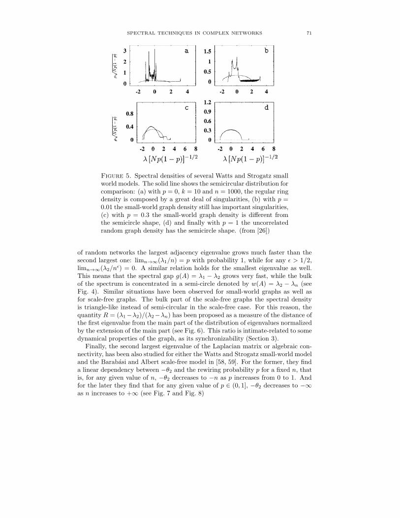
SPECTRAL TECHNIQUES IN COMPLEX NETWORKS 71
Figure 5. Spectral densities of several Watts and Strogatz smallworld models. The solid line shows the semicircular distribution forcomparison: (a) with p = 0, k = 10 and n = 1000, the regular ringdensity is composed by a great deal of singularities, (b) with p =0.01 the small-world graph density still has important singularities,(c) with p = 0.3 the small-world graph density is different fromthe semicircle shape, (d) and finally with p = 1 the uncorrelatedrandom graph density has the semicircle shape. (from [26])
of random networks the largest adjacency eigenvalue grows much faster than thesecond largest one: limn→∞(λ1/n) = p with probability 1, while for any ε > 1/2,limn→∞(λ2/n
ε) = 0. A similar relation holds for the smallest eigenvalue as well.This means that the spectral gap g(A) = λ1 − λ2 grows very fast, while the bulkof the spectrum is concentrated in a semi-circle denoted by w(A) = λ2 − λn (seeFig. 4). Similar situations have been observed for small-world graphs as well asfor scale-free graphs. The bulk part of the scale-free graphs the spectral densityis triangle-like instead of semi-circular in the scale-free case. For this reason, thequantity R = (λ1−λ2)/(λ2−λn) has been proposed as a measure of the distance ofthe first eigenvalue from the main part of the distribution of eigenvalues normalizedby the extension of the main part (see Fig. 6). This ratio is intimate-related to somedynamical properties of the graph, as its synchronizability (Section 3).
Finally, the second largest eigenvalue of the Laplacian matrix or algebraic con-nectivity, has been also studied for either the Watts and Strogatz small-world modeland the Barabasi and Albert scale-free model in [58, 59]. For the former, they finda linear dependency between −θ2 and the rewiring probability p for a fixed n, thatis, for any given value of n, −θ2 decreases to −n as p increases from 0 to 1. Andfor the later they find that for any given value of p ∈ (0, 1], −θ2 decreases to −∞as n increases to +∞ (see Fig. 7 and Fig. 8)

72 SILVIA GAGO
Figure 6. The ratio R = (λ1−λ2)/(λ2−λn) for a sparse uncorre-lated random graph (+), small-world graph with p = 0.01 (•) andscale-free network (�), versus the size of the graph n. Observethat for the first R converges to a constant, whereas for the othersdecays rapidly as n→ ∞. (from [26])
Figure 7. The opposite of the algebraic connectivity, −θ2, at twoWatts and Strogatz models as a function of the probability, for(a) n = 200 and (b) n = 500. (from [59])
The opposite of the algebraic connectivity at the Barabasi and Albert model isstudied in [58] for three cases, obtaining in all of them that −θ2 bounded functionas n increases to ∞ (Fig. 9). Observe that it has a small value, which implies thatscale-free networks have poor synchronizability (Section 3).
3. Synchronization
Synchronization is the process where two or more systems interact with eachother and come to move together. Synchronization processes are ubiquitous in na-ture and are present in many different contexts such as biology, technology, sociol-ogy, climatology, etc. The dynamics e.g., of the human cardiorespiratory system, of
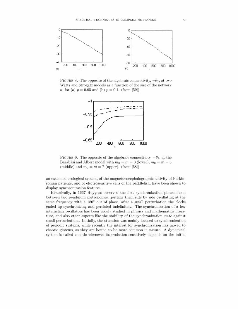
SPECTRAL TECHNIQUES IN COMPLEX NETWORKS 73
Figure 8. The opposite of the algebraic connectivity, −θ2, at twoWatts and Strogatz models as a function of the size of the networkn, for (a) p = 0.05 and (b) p = 0.1. (from [59])
Figure 9. The opposite of the algebraic connectivity, −θ2, at theBarabasi and Albert model with m0 = m = 3 (lower), m0 = m = 5(middle) and m0 = m = 7 (upper). (from [58])
an extended ecological system, of the magnetoencephalographic activity of Parkin-sonian patients, and of electrosensitive cells of the paddlefish, have been shown todisplay synchronization features.
Historically, in 1667 Huygens observed the first synchronization phenomenonbetween two pendulum metronomes: putting them side by side oscillating at thesame frequency with a 180◦ out of phase, after a small perturbation the clocksended up synchronizing and persisted indefinitely. The synchronization of a fewinteracting oscillators has been widely studied in physics and mathematics litera-ture, and also other aspects like the stability of the synchronization state againstsmall perturbations. Initially, the attention was mainly focused to synchronizationof periodic systems, while recently the interest for synchronization has moved tochaotic systems, as they are bound to be more common in nature. A dynamicalsystem is called chaotic whenever its evolution sensitively depends on the initial

74 SILVIA GAGO
conditions. There are several types of synchronization features in chaotic systems:complete synchronization, lag synchronization, generalized synchronization, phaseand imperfect phase synchronization. The most studied is the complete synchro-nization, which consists of the perfect hooking of the trajectories of a system ofidentical chaotic oscillators in the course of the time.
From different theoretical frameworks considered to study the synchronizationof complex networks, their topology has turned out to play a crucial role in de-termining their dynamical behavior. Several models for real networks associatedwith complex systems are used to study relationships between the system synchro-nization and graph invariants, as well as some of the system relevant topologicalparameters. To be more precise, the Laplacian spectra and the algebraic connectiv-ity or second smallest eigenvalue of the Laplacian matrix are important factors forobtaining the synchronization state or the stability of the synchronization state forsome of these theoretical models. Their relation with other topological parametersof the network, as the diameter or the mean distance, provides some interestingconditions for existence of the synchronization. Besides, the recent appearance oflarge complex networks and the study of their dynamical characteristics, has be-come a new challenge for the scientific community. Synchronization in small-worldand scale-free networks have aroused a great deal of interest. For more informationabout synchronization theory in dynamical systems we refer the reader to reviewpapers [1, 5].
Therefore in this section we first study two of these theoretical frameworks re-lating synchronization with Laplacian eigenvalues. By using known bounds for thealgebraic connectivity θ2 and the largest Laplacian eigenvalue θn we derive boundsfor the synchronization ratio θn/θ2. And finally we take advantage of the classicaltechniques from the spectral graph theory [17] to construct a large family of highlysynchronizable networks.
Coupled identical oscillators. In the work [50] of Pecora and Caroll the stabilityof the synchronized state of a network of coupled identical oscillators is studiedby using the so-called Master Stability Function. When all the oscillators areinitially synchronized it is a crucial question to know whether this state is stablein the presence of small perturbations. The motion of a system is described by thegeneral equation
x = F (x), x ∈ Rn.
Considering linear time-continuous systems, this equation turns out into:
(3.1) xi(t) = F (xi(t)) + σ
n∑
j=1
LijH(xj(t)), i = 1, . . . , n,
where xi(t) = (xi1 (t), . . . , xin(t))T ∈ R
n represents the state variables at eachoscillator i. The first part of the equation, x(t) = F (x(t)) explains the dynamicsof each node, and the function H(x(t)) is the output function (the same at eachnode), which represents the influence of network in the oscillator i. The parameterσ is the coupling strength, and L is the Laplacian matrix. There is a completely

SPECTRAL TECHNIQUES IN COMPLEX NETWORKS 75
synchronized state if
x1(t) = x2(t) = · · · = xn(t) = s(t),
where s(t) is the desired synchronized state. When all the oscillators are initiallysynchronized, they remain synchronized until the presence of small perturbationinterferes. Now the question is whether the synchronization state is stable in thepresence of small perturbations δxi. In this case xi(t) = s(t) + δxi, and expandingthe functions F andH to first order in a Taylor series, i.e., F (xi) = F (s)+DF (s)δxiand H(xi) = H(s)+DH(s)δxi, where DF (s) and DH(s) are the Jacobian matricesof L and H on s respectively, we obtain the following variational linear equationsfor δxi
δxi = DF (s) + σDH(s)
n∑
j=1
Lijδxj , i = 1, . . . , n.
By projecting δfxi into the eigenspaces spanned by the eigenvectors vi of theLaplacian matrix L, the former equations that can be diagonalized into blocks as
y(t) = [DF (s) + θDH(s)]y(t),
where y represents the different perturbation modes from the synchronized state,θ = σθi for each i-block, with θi the i-th eigenvalue of the Laplacian matrix, i =1, . . . , n. The idea is to project δxi into the eigenspace spanned by the eigenvectorsvi of the coupling matrix L.
The linear stability of the synchronized state for any linear coupling is providedby the largest Lyapunov exponent of this equation Δ(θ). In [50] it is shown thatthe synchronization state is stable if Δ(σθi) < 0 for i = 2, . . . , n. Moreover, it hasbeen found [3] that for many chaotic oscillators there exists a range of values in theinterval (α1, α2) where this condition is satisfied. In this case, there exists a valueof the coupling strength σ such that the synchronization state is linearly stable ifand only if
θn/θ2 < α2/α1 ≡ β,
where β is a constant independent of the Laplacian matrix L. The values for βdepend on the different kind of oscillator, but for many chaotic oscillators they useto be between 5 and 100 [50]. Therefore, for large values of θn/θ2 it is not possibleto obtain synchronization, independently of the value of the coupling strength andthe kind of oscillator.
Furthermore, Wang and Chen in a former paper [58], study the asymptoticalsynchronization of a dynamical network model characterized by Equation 3.1 withH(xj(t)) = −xj(t). It is said that the dynamical system reaches a state of asymp-totical synchronization if
x1(t) = · · · = xn(t) = s(t),
when t→ ∞, where s(t) can be an equilibrium point, a periodic orbit, or a chaoticattractor. They show that the system is exponentially stable if 1/θ2 is bounded bya constant.
In both models we can see that the synchronization of the network depends onalgebraic connectivity θ2. When it is close to 0, 1/θ2 is large, then the network
76 SILVIA GAGO
cannot reach a synchronization state. Besides, in the first model the largest Lapla-cian eigenvalue θn has also a great influence, and more precisely the ratio θn/θ2,should also be small to attain synchronizability. Nevertheless, these two Laplacianeigenvalues by themselves do not provide information about the relationship be-tween the network topology and the dynamics of synchronization. In the followingsubsection we will study some spectral bounds obtained from the classical spec-tral graph theory that will provide a connection between the synchronization of anetwork and several of its main invariants and parameters.
3.1. Synchronization and topological parameters. In order to characterize thesynchronization of a network, we study the relationship between the inverse of thesecond eigenvalue of the Laplacian matrix, 1/θ2, and the ratio θn/θ2, with othergraph topological parameters like the minimum and maximum degrees, diameter,mean distance, isoperimetric number, betweenness centrality and clustering param-eter. Most of these bounds can be found in [16]. From the bounds that can beobtained for 1/θ2 and by using the classical bound Δ < θn � 2Δ provided byFiedler [27] we can derive new lower and upper bounds for the synchronizationratio θn/θ2.
Minimum and maximum degrees of the graph. The minimum degree of a graph,δ, is related to the minimum connectivity of the graph. As θ2 � δn/(n− 1), andθn � (Δ + 1) (see [36]), one can be obtain
(1− 1
n
) (Δ + 1)
δ� θnθ2.
When the difference between the maximum and minimum degree is large (het-ereogenity), the synchronizability will be not reached. Now considering scale-freenetworks, for which δ = 1, and Δ, n are large then 1−1/n 1, and (Δ+1) � θn/θ2,which means that the network has a very low synchronization capability.
Edge connectivity. From a bound in [27] it can be easily obtained:
θnθ2
� Δ
e(G)(1− cos π
n
) .
Observe that when n is large the bound becomes independent of the value of e(G),which does not provide much information.
Diameter. One of the bounds relating the algebraic connectivity with the diam-eter was given by Mohar in [43] as D � 4/(nθ2) and so we obtain:
θnθ2
� nDΔ
2.
For graphs with a large D or n, this equation provides a large upper bound. How-ever, if both values are small then the network will be easy to synchronize. A lowerbound for the inverse algebraic connectivity can be obtained from the diameterbound D � 2
⌈Δ+θ24θ2
ln(n − 1)⌉from [43], where Δ is the maximum degree of the
graph:( 4
ln(n− 1)
⌊D2
⌋− 1)(Δ + 1)
Δ� θnθ2.
SPECTRAL TECHNIQUES IN COMPLEX NETWORKS 77
From the former equation, note that if D � ln(n − 1), then the bound is greaterthan 1, and it will be difficult to reach a synchronization state provided that themaximum degree Δ is very large.
Now, consider the following bound in [43]: if there are two subsets of vertices,B and C, at distance r + 1:
4(r − 1)2|B||C|
(n− |B| − |C|) · (|B|+ |C|) <θnθ2,
where |B| are |C| are the cardinalities of the subsets. If both subsets have only onevertex and they are at maximum distance D, the bound results
2(D − 2)2
(n− 2)<θnθ2.
For large n and a small D the bound will tend to 0 and synchronization is possible.Also, for graphs with a diameter close to n would lead to large lower bound andthe networks will not synchronize.
Studies about the diameter in small-world networks show that many real net-works associated with complex systems have a logarithmic diameter D ∼ lnn (sim-ilar to). In this case, the lower bound can be written approximately as 1/Δ � 1/θ2.Since the maximum degree Δ is also large, in scale-free networks the lower boundwill approach 0 and synchronization is possible.
Mean distance. In [43] several bounds relating the mean distance with the al-gebraic connectivity can be found. Firstly we find this bound relating the meandistance with Q:
l <n
n− 1
⌈
1 +
√θnθ2
√α2 − 1
4α
⌉(12+⌈logα
n
2
⌉),
where α > 1 is a parameter. A large mean distance hinders the network synchro-nization. A lower bound can be obtained from
l � n
n− 1
(⌈Δ+ θ24θ2
ln(n− 1)⌉+
1
2
),
(⌊2l(n− 1)− n
2n ln(n− 1)
⌋− 1
4
)4(Δ + 1)
Δ� θnθ2.
Note that as n becomes large, the bound takes a lower value if the mean distance isalso small. However, if n is small and l relatively large, the bound is also large andthe synchronization of the network would not be possible. The maximum degreealso is an influence on the synchronization, larger degrees make it easier.
Isoperimetric number of a graph or Cheeger constant. In [42] we find two differentbounds for the isoperimetric number. The lower bound i(G) � θ2/2, gives us
Δ + 1
2i(G)� θnθ2.
From this bound, if the isoperimetric number is near 0, the network will be easyto disconnect in two parts and by using the previous bound the inverse algebraicconnectivity will be large, and the synchronization would not be possible. Cheeger

78 SILVIA GAGO
inequalities relate the isoperimetric number of a graph with its algebraic connectiv-ity θ2 and its maximum degree Δ. From the upper bound i(G) �
√θ2(2Δ− θ2),
we have the inequality θ22 − 2Δθ2 + i(G)2 � 0 which leads us to
2
1 +√1− (i(G)/Δ)2
� θnθ2
� 2
1−√1− (i(G)/Δ)2.
In this case, if i(G) ∼ Δ, then both bounds in reach 2 and the synchronizationshould be possible, meanwhile i(G) ∼ 0 the lower bound goes to infinity and thenetwork cannot synchronize.
Betweenness centrality and maximum betweenness centrality. The maximumbetweenness centrality, Bmax, is larger than B, so the corresponding lower boundscan also be used to obtain lower bounds. Moreover, in [15] a bound can be foundthat relates Bmax to the isoperimetric number:
Bmax + 2 � n√θ2(2Δ− θ2)
.
Therefore it can be easily deduced that
Δ
Δ +√Δ2 − (n/(Bmax + 2))2
� θnθ2
� 2Δ
Δ−√Δ2 − (n/(Bmax + 2))2.
Observe that if (Bmax + 2)/Δ ∼ n, then θn/θ2 � 2 and synchronization ispossible, but if Bmax+2 ∼ 2n(n−1)+2 (as in a star graph), then 1/2Δ � 1/θ2 � ∞and the bounds are not useful to describe the synchronizability of a network.
The following lower and upper bounds are given in [49]:(1− 1
n
)Δδ
� θnθ2
� (n− 1)ΔBEmaxDl,
where BEmax is the maximum edge betweenness of the network [15, 33]. From the
lower bound it can be deduced that the heterogeneity of degrees affects the synchro-nization of the network. A large difference between the maximum and minimumdegrees makes the network more difficult to synchronize, which uses to happenin scale-free networks. However, homogeneous networks not always synchronize.Several studies on model networks corroborate this result in [30].
3.2. Design of synchronizable networks. As seen in previous sections, both scale-free and small-world networks display better synchronization than regular graphs[3]. However, it has also been observed that networks with strong heterogeneity inthe degree distribution are much more difficult to synchronize than random homo-geneous networks [49]. Donetti et al. in [19, 20] proposed entangled networks, whichare extremely homogeneous regular networks, as examples of highly synchronizablenetworks. These graphs are obtained by using a numerical optimization algorithm,which excludes the possibility of using mathematical tools to generate infinitelymany such networks. However, Estrada et al. [24, 7] propose a different approach,introducing a family of graphs (golden spectral graphs) which can be built by usinganalytical tools from the classical algebraic graph theory [17].

SPECTRAL TECHNIQUES IN COMPLEX NETWORKS 79
Observe that for a regular graph the synchronization ratio is related with R by
Q =θnθ2
=λ1 − λnλ1 − λ2
=λ2 − λnλ1 − λ2
· λ1 − λnλ2 − λn
= ω1(G) · ω2(G) =1
R· (R + 1),
where
ω1(G) =λ2 − λnλ1 − λ2
, λ1 �= λ2, ω2(G) =λ1 − λnλ2 − λn
, λ2 �= λn,
are inverse, and therefore it is not easy to find graphs in which their product issmall. This fact clearly hampers the synchronization of the network. In the searchof graphs with small Q = ω1(G) · ω2(G), we consider those where both spectralratios are equal, as it is straightforward to check that in this case ω1(G) = ω2(G) =
ϕ = (1 +√5)/2 and thus Q = ϕ2 = ϕ+ 1.
Definition 3.1. A golden spectral graph (GSG) is a graph for which both spectralratios are identical, that is
ω1(G) = ω2(G) = ϕ,
where ϕ = (1 +√5)/2 is the golden section, golden mean or divine proportion.
The first examples and properties of golden spectral graphs are found by Estradain [7] and amplified in [24] by using classical spectral techniques, finding infinitefamilies of such graphs (see Fig. 10).
Figure 10. Two examples of highly synchronizable networks:C5 ⊗ J3 and the icosahedral graph.
4. Community detection and spectral bisection
Empirical studies reveal a common property between many networks: commu-nity structure, i.e., the division of network vertices into groups with dense connec-tions between them and sparse connections between groups [33, 47]. Communitiesare important because they often correspond to functional units such as cyclesor pathways in metabolic networks or collections of pages on a single topic on theweb. Moreover, networks can have properties at the community level that are quitedifferent for the entire network.

80 SILVIA GAGO
A huge variety of community detection techniques have been developed, based oncentrality measures, spectral techniques, flow models, random walks, resistor net-works, optimization and many other approaches [18, 47]. There is a large literatureabout finding connections between divisions of networks and matrix spectra, theso-called spectral partition or spectral clustering [56]. The main tools for spectralclustering are graph Laplacian matrices or normalized Laplacian matrices. Mostapproaches to graph partitioning are based on iterative bisection methods, that is,finding the best division of the graph into two groups and then further subdividingthose two into more groups. The spectral bisection method is originally due toFiedler [27] and popularized by Pothen et al. [51], and is based on the Laplacianmatrix eigenvectors. We describe here the simplest form of this method.
For dividing the graph into two subgraphs it is usual to consider the followingparameter:
Definition 4.1. Given two subsets A and B of the vertex set V (G) of a graph Gand forming a partition of it, the number of edges connecting them is called thecut size
(4.1) R =1
2
∑
i∈A, j∈B
ai,j ,
where the factor 1/2 compensates for counting each edge twice.
Now consider an index vector s with n elements as
(4.2) si =
{1, if i ∈ A,
−1, if i ∈ B.
Observe that sT s = n, and
1
2(1− sisj) =
{1, if i and j are in different groups,0, if i and j are in the same group.
This allows us to rewrite Equation 4.1 as
R =1
4
∑
i, j∈V (G)
(1− sisj)ai,j .
Recalling that the degree of a vertex i is ki =∑
j aij , then
∑
i,j∈V (G)
aij =∑
i∈V (G)
ki =∑
i∈V (G)
s2i ki =∑
i,j∈V (G)
sisjkiδij ,
where δij = 1 if i = j and 0 otherwise. Therefore
R =1
4
∑
i,j∈V (G)
sisj(kiδij − ai,j) =1
4sTLs.
Considering an orthogonal basis of Laplacian eigenvectors vi, for 1 � i � n, the in-dex vector s can be expressed as a linear combination of the Laplacian eigenvectors,
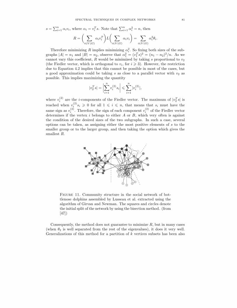
SPECTRAL TECHNIQUES IN COMPLEX NETWORKS 81
s =∑n
i=1 αivi, where αi = vTi s. Note that∑n
i=1 α2i = n, then
R =
( ∑
i∈V (G)
αivTi
)L
( ∑
i∈V (G)
αivi
)=
∑
i∈V (G)
α2i θi.
Therefore minimizing R implies minimizing α2i . So fixing both sizes of the sub-
graphs |A| = n1 and |B| = n2, observe that α21 = (vT1 s)
2 = (n1 − n2)2/n. As we
cannot vary this coefficient, R would be minimized by taking s proportional to v2(the Fiedler vector, which is orthogonal to vi, for i � 3). However, the restrictiondue to Equation 4.2 implies that this cannot be possible in most of the cases, buta good approximation could be taking s as close to a parallel vector with v2 aspossible. This implies maximizing the quantity
|vT2 s| =∣∣∣∣
n∑
i=1
v(2)i si
∣∣∣∣ �
n∑
i=1
|v(2)i |,
where v(2)i are the i-components of the Fiedler vector. The maximum of |vT2 s| is
reached when v(2)i si � 0 for all 1 � i � n, that means that si must have the
same sign as v(2)i . Therefore, the sign of each component v
(2)i of the Fiedler vector
determines if the vertex i belongs to either A or B, which very often is againstthe condition of the desired sizes of the two subgraphs. In such a case, severaloptions can be taken, as assigning either the most positive elements of s to thesmaller group or to the larger group, and then taking the option which gives thesmallest R.
Figure 11. Community structure in the social network of bot-tlenose dolphins assembled by Lusseau et al. extracted using thealgorithm of Girvan and Newman. The squares and circles denotethe initial split of the network by using the bisection method. (from[47])
Consequently, the method does not guarantee to minimize R, but in many cases(when θ2 is well separated from the rest of the eigenvalues), it does it very well.Generalizations of this method for a partition of k vertices subsets has been also

82 SILVIA GAGO
studied, and besides using other kinds of Laplacian matrices. For an extensivestudy about this subject we refer the reader to [56].
However, the method is a poor tool for detecting natural community structurein real-world networks, as the sizes of the groups are fixed from the beginning.Several approaches have been proposed to solve this problem. For this reason,Girvan and Newman [33] implemented an algorithm for calculating the modularityof the network, a new measure of how good is a particular division of the networkis (see Fig. 11). That is, for a division with k groups, consider the k × k matrix Ewhose component eij is the fraction of edges in the original network that connectvertices in group i to those in group j. Then the modularity index is defined as
Q =∑
i
eii −∑
ijk
eijeki.
Physically Q is the fraction of all edges that lie within communities minus the ex-pected value of the same quantity in a graph in which the vertices have the samedegrees but where edges are placed at random without regard for the communi-ties. If Q = 0 the community structure is not stronger than the one that can beexpected by random chance. Local peaks in the modularity during the progressof the community structure algorithm indicate particularly good divisions of thenetwork.
Modularity can also be approached by spectral methods. In [48] three spectraltechniques can be found for approximating this parameter: the leading eigenvectormethod, other eigenvectors of the modularity matrix and a vector partitioningalgorithm. All of them follow similar spectral techniques to the ones used in thefirst part of this section.
References
[1] A. Arenas, A. Dıaz-Guilera, J. Kurths, Y. Moreno, C. Zhou, Synchronization in complexnetworks, Phys. Rep. 469 (2008), 93–153.
[2] A. L. Barabasi, R. Albert, Emergence of scaling in random networks, Science 286 (1999),509-512.
[3] M. Barahona, L.M. Pecora, Synchronization in small-world systems, Phys. Rev. Lett. 89(2002), 054101.
[4] S. Boccaletti, J. Kurths, G. Osipov, D. L. Valladares, C. S. Zhou, The synchronization ofchaotic systems, Phys. Rep. 366 (2002), 1-101.
[5] S. Boccaletti, V. Latora, Y. Moreno, M. Chavez, D.U. Hwang, Complex networks: Structureand dynamics, Phys. Rep. 424 (2006), 175-308.
[6] A. Bonato, J. Jensen, A survey of models of the web graph, Proceedings of Combinatorialand Algorithmic Aspects of Networking, (2004).
[7] G. Caporossi, E. Estrada, S. Gago, Design of highly-synchronizable and robust networks,Automatica (2010), in press.
[8] Q. Chen, H. Chang, R. Govindan, S. Jamin, S. Shenker, W. Willinger, The Origin of PowerLaws in Internet Topologies Revisited, in: Proc. INFOCOM, New York, USA, 2002, 608–617.
[9] C.K. Cheng, Y.C. Wei, An improved two-way partitioning algorithm with stable performance,IEEE Trans CAD 10 (1991), 1502–1511.
[10] F.R.K. Chung, L. Lu, Complex graphs and networks, American Mathematical Society 107(2006).
SPECTRAL TECHNIQUES IN COMPLEX NETWORKS 83
[11] F.R.K. Chung, L. Lu, V. Vu, The spectra of random graphs with given expected degrees,Proc. Natl. Acad. Sci. 100 (2003), 6313-6318.
[12] F.R.K. Chung, L. Lu, V. Vu, Eigenvalues of random power law graphs, Annals of Combina-torics 7 (2003), 21-33.
[13] F. Comellas, S. Gago, A star based model for the eigenvalue power law of Internet graphs,Phys. A 351 (2005), 680–686.
[14] F. Comellas, Complex Networks: Deterministic Models, in: J. P. Gazeau et al. (ed.), Physicsand Theoretical Computer Science, IOS Press, Amsterdam, (2007), 275–293.
[15] F. Comellas, S. Gago, Spectral bounds for the betweenness of a graph, Linear Algebra Appl.423 (2007), 74–80.
[16] F. Comellas, S. Gago, Synchronizability of complex networks, J. Phys. A: Math. Theor. 40(2007), 4483-4492.
[17] D. Cvetkovic, M. Doob, H. Sachs, Spectra of Graphs, Academic Press, New York, 1979.[18] L. Danon, A. Dıaz-Guilera, J. Duch, A. Arenas, Comparing community structure identifica-
tion, J. Stat. Mech. Theor. Exp. 2005, 09008.[19] L. Donnetti, P. I. Hurtado, M.A. Munoz, Entangled networks, synchronization, and optimal
network topology, Phys. Rev. Lett. 95 (2005), 188701.[20] L. Donnetti, P. I. Hurtado, M. A. Munoz, Optimal network topologies: expanders, cages,
Ramanujan graphs, entangled networks and all that, J. Stat. Mech. P (2006), 08007.[21] R. Elsasser, Toward the Eigenvalue Power Law, Lect. Notes. Comput. Sci. 4162 Springer-
Verlag, Berlin (2006), 351-362.[22] P. Erdos, A. Renyi, On Random Graphs I, Publ. Math. 6 (1959), 290-297.[23] E. Estrada, Spectral Theory of Networks: From Biomolecular to Ecological in: M. Dehmer,
F. Emmert-Streib (eds.), Analysis of Complex Networks. From Biology to Linguistics, Wiley-VCH,Weinheim (2009), 145–174.
[24] E. Estrada, Graphs(networks) with golden spectral ratio, Chaos, Solitons and Fractals 33(2007), 1168–1182.
[25] M. Faloutsos, P. Faloutsos, C. Faloutsos, On power-law relationships of the internet topology,Proceedings of the Conference SigComm, ACM (1999).
[26] I. J. Farkas, I. Dereenyi, A. L. Barabasi, T. Vicsek, Spectra of real-world graphs: Beyond thesemicircle law, Phys. Rev. E 64 (2001), 026704.
[27] M. Fiedler, Algebraic connectivity of graphs, Czech. Math. J. 23 2 (1973), 298-305.[28] A. Flaxman, A. Frieze, T. Fenner, High Degree Vertices and Eigenvalues in the Preferential
Attachment Graph, Internet Mathematics 2 1 (2005), 1–19.[29] L.C. Freeman, A set of measures of centrality based upon betweenness, Sociometry 40 (1977),
35–41.
[30] H. Hong, B. J. Kim, M.Y. Choi, H. Park, Factors that predict better synchronizability oncomplex networks, Phys. Rev. E 69 (2004), 067105.
[31] S. Gago, Eigenvalue distribution in power law graphs, Aplimat-Journal of Applied Mathe-matics, 1 1 (2008), 30–36.
[32] S. Gago, J. Hurajova, T. Madaras, Notes on betweenness centrality of a graph, Math. Slov.(2010), to appear.
[33] M. Girvan, M.E. J. Newman, Community structure in social and biological networks, Proc.Natl. Acad. Sci. U.S.A. 99 (2002), 7821.
[34] C. Gkantsidis, M. Mihail, E. Zegura, Spectral analysis of internet topologies, in: Proceedingsof Infocom, San Francisco, CA, 1, March (2003), 364–374.
[35] K. I. Goh, B. Kahng, D. Kim, Universal behavior of load distribution in scale-free networks,Phys. Rev. Lett. 87 2001, 278701.
[36] R. Grone, R. Merris, The Laplacian spectrum of a graph II, SIAM J. Discrete Math. 7 (1994),221–9.
[37] A. Jamakovic, S. Uhlig, On the relationship between the algebraic connectivity and graphsrobustness to node and link failures, in: Next Generation Internet Networks 3rd EuroNGIConference on Trondheim, Norway (2007).
84 SILVIA GAGO
[38] D. Kim, B. Kahng, Spectral densities of scale-free networks, Chaos 17 (2007), 026115.[39] J. Kleinberg, S. R. Kumar, P. Raphavan, S. Rajagopalan, A. Tomkins, The web as a graph:
Measurements, models and methods, in: Proceedings of the International Conference onCombinatorics and Computing, 1999.
[40] P.N. McGraw, M. Menzinger, Clustering and synchronization of oscillator networks, Phys.Rev. E 72 (2005), 015101.
[41] M. Mihail, C. Papadimitriou, On the Eigenvalue Power Law, Lect. Notes Comput. Sci. 2483(2002), 254–262.
[42] B. Mohar, Isoperimetric number of graphs, J. Combin. Theory Ser. B 47 (1989), 274–91.[43] B. Mohar, Eigenvalues, diameter and mean distance in graphs, Graphs Combin. 7 (1991),
53–64.[44] M. Najiminaini, L. Subedi, Lj. Trajkovic, Analysis of Internet topologies: a historical view,
in: Proc IEEE Int. Symp. Circuits and Systems, Taipei, Taiwan, (2009), 1697–1700.[45] M.E. J. Newman, The Structure and Function of Complex Networks, SIAM Rev. 45 2 (2003),
167-256.[46] M.E. J. Newman, Models of the Small World, J. Stat. Phys. 101 (2000), 819–841.[47] M.E. J. Newman, Detecting community structure in networks, Eur. Phys. J. B 38 (2004),
321-330.[48] M.E. J. Newman, Finding community structure in networks using the eigenvectors of matri-
ces, Phys. Rev. E 74 (2006), 036104.[49] T. Nishikawa, A.E. Motter, Y.C. Lai, F.C. Hoppensteadt, Heterogeneity in oscillator net-
works: are smaller worlds easier to synchronize?, Phys. Rev. Lett. 91 (2003), 014101.[50] L.M. Pecora, T. L. Carroll,Master stability functions for synchronized coupled systems, Phys.
Rev. Lett. 80 (1998), 2109–12.[51] A. Pothen, H.D. Simon, K.P. Liou, Partitioning sparse matrices with eigenvectors of graphs,
SIAM J. Matrix Anal. Appl. 11 3 (1990), 430–452.[52] G. Siganos, M. Faloutsos, P. Faloutsos, C. Faloutsos, Power-Laws and the AS-level Internet
Topology, IEEE/ACM Transactions on Networking 11 4 (2003), 514–524.[53] L. Subedi, L. Trajkovic, Spectral Analysis of Internet Topology Graphs, IEEE Int. Symp.
Circuits and Systems, Paris, France, May 2010.[54] E.R. van Dam, Regular graphs with four eigenvalues, Linear Alg. Appl. 226-228 (1995),
139–162.[55] P. van Mieghem, Graph Spectra for Complex Networks, Cambridge University Press, Cam-
bridge, to appear.[56] U. von Luxburg, A Tutorial on Spectral Clustering, Statistics and Computing 17(4) (2007),
395–416.
[57] D. Vukadinovic, P. Huang, T. Erlebach, A Spectral Analysis of the Internet Topology, ETHTIK-NR. 118, July 2001.
[58] X. F. Wang, G. Chen, Synchronization in scale-free dynamical networks: robustness andfragility, IEEE Trans. Circuits Sys. I 49 (2002), 54–62.
[59] X. F. Wang, G. Chen, Synchronization in small-world dynamical networks, Int. J. BifurcationChaos 12 1 (2002), 187-192.
[60] D. J. Watts, S.H. Strogatz, Collective dynamics of small-world networks, Nature 393 (1998),440-442.
[61] E.P. Wigner, On the Distribution of the Roots of Certain Symmetric Matrices, Ann. of Math.67 (1958), 325–328.
[62] C.W. Wu, L.O. Chua, Application of Graph Theory to the Synchronization in a Array ofCoupled Nonlinear Oscillators, IEEE Trans. Circuits Sys. I 42 (1995), 494–7.

Dragan Stevanovic
APPLICATIONS OF GRAPH SPECTRAIN QUANTUM PHYSICS
Abstract. Graph spectra are closely related to many applications inquantum physics: a network of quantum particles with fixed couplingscan be modelled by an underlying graph, with the Hamiltonian ofsuch system approximated by the adjacency matrix of that graph,and the energy levels and states represented by the eigenvalues andeigenvectors of the adjacency matrix. From that viewpoint, quite afew quantum physics problems can be posed in terms of the spectralproperties of the graph. In this chapter we survey one particularproblem which received a lot of attention recently: the existence ofperfect state transfer in the network of spin-1/2 particles.
Mathematics Subject Classification (2010): Primary: 05-02, 05C50;Secondary 81P68
Keywords : Quantum spin system; Perfect state transfer.
Contents
1. Introduction 862. Basics of quantum mechanics 873. Perfect transfer of quantum states 904. Consequences of perfect state transfer on relations between vertices 935. Eigenvalue ratio condition and periodic graphs 946. Some regular graphs with perfect state transfer 967. Cartesian product of graphs 978. Cubelike graphs 999. Integral circulant graphs 10010. Other graph compositions 10311. Perfect routing of quantum states 10512. Conclusion 106References 107
1. Introduction
Graph spectra have had a long history of applications in statistical physics,through dimer problem, and in chemistry, through Huckel’s theory [31]. Here wesurvey another, more recent application of graph spectra in sciences, this timein quantum physics, through the problem of establishing perfect transfer of qubitstates in the network of spin-1/2 particles. Most of the results we review here werepublished with last six years.
After necessary initial review in Section 2 of quantum mechanical terms andnotions, assembled by a non-physicist for other non-physicists, the notion of perfectstate transfer is defined in Section 3. These two sections are the only ones dealingwith physical aspects of perfect state transfer, the rest of the survey being devotedto mathematical results. It turns out that it is not easy to find graphs admittingperfect state transfer between a pair of its vertices: in Section 4 it is shown thatany automorphism of a graph fixing one vertex must fix the other vertex as well,and that the angles of both vertices have to coincide. Among paths, only those oflengths 2 and 3 admit perfect state transfer, while it does not exist in any longerpath (Section 5). Regular, integral graphs turn out to be presently richest sourceof graphs with perfect state transfer: some particular examples are exhibited inSection 6, while the classes of cubelike and integral circulant graphs are treatedin Sections 8 and 9. From known graphs with perfect state transfer it is possible
86

APPLICATIONS OF GRAPH SPECTRA IN QUANTUM PHYSICS 87
to construct new graphs admitting perfect state transfer: the Cartesian productof graphs is best suited in this respect (Section 7), while a few more specializedconstructions are given in Section 10. In Section 11 we review a concept of routingof quantum states, which further builds upon the concept of perfect state transferand may present the source of new, interesting mathematical problems. Concludingremarks are given in Section 12.
We review here perfect state transfer in uniformly coupled spin networks (simplegraphs) only. Another aspect of perfect state transfer that we do not consider hereis its physical implementation. There is a large body of physics literature on thistopic, and most of it is listed in references, so that the interested researcher mayfind the list of references as a useful start point.
2. Basics of quantum mechanics
Bra-ket notation. Bra-ket notation was introduced in 1939 by Paul Dirac,and is also known as Dirac notation [92]. It is used to denote abstract vectorsand linear functionals in mathematics, and it is a standard notation for describingquantum states in the theory of quantum mechanics. It is called bra-ket becausethe inner product of two states (vectors) is denoted by a bracket, 〈x|y〉, consistingof a left part bra, 〈x|, and a right part ket, |y〉. The bra 〈x| represents a row vectorxT , while the ket |y〉 represents a column vector y. Thus, 〈x|y〉 is same as xT y. IfA : H → H is a linear operator, applying A to the ket |y〉 gives a new ket A|y〉.Thus, 〈x|A|y〉 is same as xTAy.
Classical and quantum description of mechanics A physical system isgenerally described by three basic ingredients: states; observables; and dynamics(or law of time evolution) or, more generally, a group of physical symmetries. Aclassical description can be given in a fairly direct way by a phase space modelof mechanics: states are points in a symplectic phase space, observables are real-valued functions on it, time evolution is given by a one-parameter group of sym-plectic transformations of the phase space, and physical symmetries are realized bysymplectic transformations [93].
In a quantum description, each physical system is associated with a (topolog-ically) separable complex Hilbert space H with inner product 〈x|y〉. Rays (one-dimensional subspaces) in H are associated with states of the system. In otherwords, physical states can be identified with equivalence classes of unit vectorsin H, where two vectors represent the same state if they differ only by a phase fac-tor. Physical observables are represented by densely-defined self-adjoint operatorson H. The expected value of the observable A for the system in state representedby the unit vector |ψ〉 ∈ H is 〈ψ|A|ψ〉. The possible values of the observable A inany state must belong to the spectrum of A, and in the special case A has onlydiscrete spectrum, the possible outcomes of measuring A are its eigenvalues.
Schrodinger equation and Hamiltonian The time evolution of the state isgiven by a differentiable function from R, representing instants of time, to theHilbert space of system states. The Schrodinger equation [91] says that, if |ψ(t)〉

88 DRAGAN STEVANOVIC
denotes the state of the system at any one time t, then
H |ψ(t)〉 = i�d
dt|ψ(t)〉,
where H is a densely-defined self-adjoint operator, called the system Hamiltonian,i is the imaginary unit, and � is reduced Planck’s constant. As an observable, Hcorresponds to the total energy of the system.
The Hamiltonian generates the time evolution of quantum states. Given thestate at some initial time (t = 0), we can integrate Schrodinger equation to obtainthe state at any subsequent time. In particular, if H is independent of time, then
|ψ(t)〉 = e−itH� |ψ(0)〉.
As everything in quantum setting is quantized in terms of �, it is usual to assume� = 1 so that times and energies can be treated as dimensionless. The operators
U(t) = e−itH =∑
n�0
intnHn
n!
form a one-parameter unitary group U(t) : H → H, which realize physical symme-tries of the closed quantum system.
Spin Experiments show that most subatomic particles have a permanent, built-in angular momentum, which is not due to their motion through space. Thisquantity is called the spin [91], and it has no correspondence at all in conventionalphysics. The spin σ comes in units of �/2 and it belongs to the discrete set ofvalues: σ ∈ {−S�,−(S − 1)�, . . . ,+(S − 1)�,+S�}, where S is the spin quantumnumber of a particle. All elementary particles of a given kind have the same spinquantum number S. One distinguishes bosons (S = 0, 1, 2, . . . ) and fermions (S =12 ,
32 ,
52 , . . . ). Quanta of light are bosons with S = 1 and electrons are fermions with
S = 1/2.
Qubit The unit of quantum information—the quantum analogue of the classicalbit—is a quantum bit, or qubit [1, 95]. Contrary to a classical bit, the qubit isdescribed by state of a spin- 12 particle (although any two-level quantum system,such as quantum dot, may be used to describe qubit). The qubit has two basisstates in which its spin can be measured: |0〉 corresponding to spin − 1
2 , and |1〉corresponding to spin + 1
2 . A pure qubit state is a linear combination of |0〉 and |1〉,|ψ〉 = α|0〉+ β|1〉,
where α, β ∈ C are probability amplitudes. When we measure this qubit in thestandard basis, the probability of outcome |0〉 is |α|2 and the probability of outcome|1〉 is |β|2 (thus, |α|2+ |β|2 = 1). Note, however, that when we measure the state ofthe qubit we alter the values of α and β: for instance, if the state |0〉 is measured,α is changed to 1 (up to phase) and β is changed to 0.
Geometrically, the state space of a single qubit can be represented by the Blochsphere. This is a two-dimensional space which has an underlying geometry of thesurface of a sphere, meaning that the single qubit register space has two localdegrees of freedom. Represented on such a sphere, a classical bit could only be on

APPLICATIONS OF GRAPH SPECTRA IN QUANTUM PHYSICS 89
Figure 1. Bloch sphere.
the z-axis at the top or bottom of the sphere, in the locations where |0〉 and |1〉are. The rest of the surface is inaccessible to a classical bit.
Unitary transformations that can be performed on pure qubit states correspondto rotations of the Bloch sphere. These rotations can be represented as combina-tions of rotations about the x-axis (σx), the y-axis (σy), or the z-axis (σz). Forspin- 12 particles, these basic rotations are represented by three Pauli matrices:
σx =
(0 11 0
), σy =
(0 −ii 0
), σz =
(1 00 −1
).
Each Pauli matrix is an observable describing the spin of a particle in the threespatial directions.
Quantum computing A quantum computer is a computation device thatmakes direct use of quantum mechanical properties, such as superposition andentanglement, to represent data and perform operations on them [94]. Althoughquantum computing is still in its infancy, experiments have been carried out inwhich quantum computational operations were executed on a very small numberof qubits. If large-scale quantum computers can be built, they will be able tosolve certain problems much faster than any current classical computers (for ex-ample Shor’s algorithm for prime factorization). Quantum computer do not allowthe computations of functions that are not theoretically computable by classicalcomputers, i.e., they do not alter the Church-Turing thesis. The gain is only inefficiency.
Quantum computers only run probabilistic algorithms. A quantum computer issaid to solve a problem if, for every instance, its answer will be right with highprobability. In classical randomized computation, the system evolves according tothe application of stochastic matrices, which preserve that the probabilities add upto one (i.e., preserve the l1 norm). In quantum computation, allowed operationsare unitary transformations, which are effectively rotations. They preserve that

90 DRAGAN STEVANOVIC
the sum of the squares add up to one, the Euclidean or l2 norm). Consequently,since rotations can be undone by rotating backward, quantum computations arereversible.
When algorithm terminates, the result needs to be read off from a memoryregister. In a classical computer, which has a memory made up of bits, we samplefrom the probability distribution on the n-bit register to obtain one definite n-bit string. The memory register in a quantum computer is made up of n qubits,such that the state of each qubit is encoded with the state of the correspondingspin- 12 particle. We read the quantum register by measuring qubit states, which isequivalent to collapsing the quantum state down to a classical distribution (withthe coefficients in the classical state being the squared magnitudes of the coefficientsfor the quantum state) followed by sampling from that distribution. Note that nqubits can be in an arbitrary quantum superposition of up to 2n different statessimultaneously—this is a true advantage over classical computer which can only bein one of these 2n states at any one time.
3. Perfect transfer of quantum states
An important task in quantum-information processing is the transfer of quan-tum states from one location (u) to another location (v). In general, photons areexcellent flying qubits as they can be transmitted coherently over very large dis-tances [38, 61], and optical systems, often employed in quantum communicationand cryptography applications, transfer quantum states from u to v directly viaphotons [11, 12]. Thus, one possibility to transfer the quantum state is that itis imprinted onto a photon which is then used as the flying qubit over an opticalfiber. However, it is very difficult to realize such transfer in solid-state quantumsystems, as it requires perfect interface betwen photons and the main hardware ofthe quantum computer, and may not be worth it for short-distance communication(e.g., between two quantum processors).
Another way to accomplish quantum state transfer at short distance is by multi-ple applications of controlled swap operations along the communication line. How-ever, every external manipulation inevitably induces noise in the system. It istherefore desirable to minimize the amount of external control on the system, tothe point that it is not needed at all during the transfer. In such case, a quantumwire, the most fundamental unit of any quantum processing device, is made out ofmany interacting components [14, 28]. There are various physical systems that canserve as quantum wires, one of them being a quantum spin system. It is generallydefined as a network of interacting qubits, whose dynamics is governed by a suitableHamiltonian, e.g., the Heisenberg or XY Hamiltonian.
A quantum spin system is obtained by attaching a spin- 12 particle to each vertexof a connected, finite graph G = (V,E). To each vertex i ∈ V , one can associate aHilbert space Hi
∼= C2, so that the Hilbert space associated with G is given by
HG =⊗
i∈V
Hi∼= (C2)⊗n,

APPLICATIONS OF GRAPH SPECTRA IN QUANTUM PHYSICS 91
where n = |V | is the number of vertices in G. The dynamics of the system isgoverned by the XY Hamiltonian
HG =1
2
∑
(i,j)∈E(G)
Jij [σxi σ
xj + σy
i σyj ],
where the symbols σxi , σ
yi and σz
i denote the Pauli matrices acting on the Hilbertspace Hi, and Jij is the coupling strength between the vertices i and j of G. Thecouplings Jij represent the weights of the edges of G, so that its adjacency matrixAG is given by
Aij(G) =
{Jij , if (i, j) ∈ E0, if (i, j) /∈ E
Note that Jij = Jji since HG is Hermitian.The total z component of the spin, given by
σztot =
∑
i∈V
σzi ,
is conserved, i.e., [σztot, HG] = 0. The Hilbert space HG is then decomposed into
invariant subspaces, each of which is a distinct eigenspace of the operator σztot.
For the purpose of quantum state transfer, it suffices to restrict our attention tothe single excitation subspace SG, which is the n-dimensional eigenspace of σz
tot,corresponding to the eigenvalue 1− n
2 . The quantum states initially in SG will re-main there under time evolution. A basis state in SG corresponds to a configurationof spins in which all the spins except one are |0〉 and one spin is |1〉. Such a basisstate can hence be denoted by the ket |j〉, where j ∈ V is the vertex at which thespin is |1〉j . Thus, {|j〉 : j ∈ V } denotes a complete set of orthonormal basis vectorsspanning SG. When restricted to the subspace SG, HG is represented, in this basis,by an n × n matrix which is identical to the adjacency matrix AG. As known,the spectrum of the adjacency matrix of a graph is, by definition, the spectrum ofthe graph. In this way we see that the theory of graph spectra is relevant for theproblems that we consider, i.e. in quantum computing. Some basic information onthe theory of graph spectra can be found in the introductory chapter of this book,while further information may be found in the textbook [33].
The quantum spin system onG has the role of a (noiseless) quantum channel [28].The process of transmitting a quantum state from u to v proceeds in four steps:
(1) Initialization of the spin system to the state |0〉 := |0u0 . . . 00v〉. This is azero-energy eigenstate of HG.
(2) Creation of the quantum state |ψ〉u ∈ Hu at vertex u to be transmitted. Let|ψ〉u = α|0〉u + β|1〉u with α, β ∈ C and |α|2 + |β|2 = 1.
(3) Time evolution of the system for an interval of time, say t0.(4) Recovery of the state at vertex v.The state of the entire spin system after step (2) is given by
|Ψ(0)〉 = |ψu0 . . . 00v〉 = α|0u0 . . . 00v〉+ β|1u0 . . . 00v〉 = α|0〉+ β|u〉.Since the |0〉 component of the state |Ψ(0)〉, as the zero-energy eigenstate of HG,is invariant under the evolution, it suffices to focus on the evolution of the |u〉

92 DRAGAN STEVANOVIC
component, i.e., to the choice α = 0 and β = 1 above. This state evolves in time tto
|Ψ(t)〉 = e−iAGt|u〉 =n∑
j=1
βj(t)|j〉
with complex coefficients βj(t), where 1 =∑n
j=1 |βj(t)|2. At time t, the spin |1〉vmay be measured at vertex v with probability |βv(t)|2, where
βv(t) = 〈v|e−iAGt|u〉.Thus, we say that G has perfect state transfer from u to v in time t if
|〈v|e−iAGt|u〉| = 1.
In such case, 〈j|e−iAGt|u〉 = 0 for all j �= v. The effect of the modulus above isthat the quantum state after transfer is not exactly equal |v〉, but rather eiφ|v〉.However, the phase factor eiφ is not a problem, because φ will be a known quantityfor G, and it can be corrected for with an appropriate phase gate.
The communication distance of a graph G is the maximum distance betweenvertices u and v of G for which perfect state transfer is possible. For a fixed numberof qubits, the basic question is to find quantum spin systems which maximize thecommunication distance.
The time evolution of states in SG under the action of the Hamiltonian HG mayalso be interpreted as a continuous-time quantum walk on G, first considered byFarhi and Gutmann in 1998 [35] (see also [25]). The quantum walks are interestingin their own right due to their property of universal quantum computation [26].
Let λk and |μk〉 be the eigenvalues and the unit eigenvectors of AG, for k =1, . . . , n. Recall that, if f is a complex function defined on the eigenvalues of A,then
f(AG) =
n∑
i=1
f(λi)|μi〉〈μi|.
In particular,
e−iAGt =∑
i
e−iλit|μi〉〈μi|,
and
〈v|e−iAGt|u〉 = 〈v|{ n∑
k=1
e−iλkt|μk〉〈μk|}|u〉.
One can use this formula to check that paths with two and three vertices haveperfect state transfer between their end-vertices:
(a) For path P2 = ({1, 2}, {{1, 2}}) we have
〈1|e−iAP2 t|2〉 = −i sin t and |〈1|e−iAP2π2 |2〉| = 1.
(b) For path P3 = ({1, 2, 3}, {{1, 2}, {2, 3}}) we have
〈1|e−iAP3 t|3〉 = − sin2(t/√2) and |〈1|e−iAP3
π√2 |3〉| = 1.
APPLICATIONS OF GRAPH SPECTRA IN QUANTUM PHYSICS 93
4. Consequences of perfect state transfer on relations between vertices
Let G be a graph of the quantum spin system with unit couplings and adjacencymatrixA. Godsil [40] has recently derived few important lemmas on the relationshipbetween vertices among which perfect state transfer occurs. Let Aut(G)v denotesthe group of automorphisms of G that fix its vertex v.
Lemma 4.1. [40] If G admits perfect state transfer from u to v, then Aut(G)u =Aut(G)v.
Proof. We identify the automorphisms of G with the permutation matrices thatcommute with A. Since e−iAt is a polynomial in A, any permutation matrix fromAut(G) commutes with e−iAt. If the automorphism associated with P fixes u, thenP |u〉 = |u〉. If perfect state transfer takes place at time τ and H = e−iAτ , thenthere is γ ∈ C such that |γ| = 1 and H |u〉 = γ|v〉. So
γP |v〉 = PH |u〉 = HP |u〉 = H |u〉 = γ|v〉and thus v is fixed by P as well. Thus, Aut(G)u ⊆ Aut(G)v. The argument is samewhen we replace u and v, hence Aut(G)v ⊆ Aut(G)u as well. �
Vertices u and v of G are cospectral if φ(G− u, t) = φ(G− v, t), where φ(G, t) =∏nk=1(t − λk) is the characteristic polynomial of G. Alternatively, u and v are
cospectral if they have the same angles [32].
Lemma 4.2. [40] If G admits perfect state transfer from u to v, then u and v arecospectral.
Proof. By Cramer’s rule,
((tI −A)−1)u,u =φ(G− u, t)
φ(G, t)
and so using the spectral decomposition we find that
φ(G− u, t)
φ(G, t)=
n∑
k=1
〈μk|u〉2t− λk
.
Let θ1, . . . , θr be all distinct values among λ1, . . . , λn, and let μji , μji+1, . . . , μji+1−1
be the eigenvectors corresponding to θi, 1 � i � r. The orthogonal projection ontothe eigenspace corresponding to θi is given by
Ei =
ji+1−1∑
k=ji
|μk〉〈μk|.
Assume we have perfect state transfer from u to v at time τ and set H = e−iAτ .Then there is γ ∈ C such that |γ| = 1 and H |u〉 = γ|v〉. Since H is a polynomialin A, it commutes with each projection Ei and therefore
γEi|v〉 = EiH |u〉 = HEi|u〉.

94 DRAGAN STEVANOVIC
As H is unitary, this implies that Ei|v〉 and Ei|u〉 have the same length, i.e.,
ji+1−1∑
k=ji
〈μk|v〉2 =
ji+1−1∑
k=ji
〈μk|u〉2.
From this we conclude that G−u andG−v have the same characteristic polynomial.Thus u and v are cospectral. �
5. Eigenvalue ratio condition and periodic graphs
We say that G is periodic relative to the vertex u if there is a time t such that
|〈u|e−iAt|u〉| = 1.
We say that G is periodic if there is a time t such that e−iAt is diagonal, i.e., if Gis periodic relative to each of its vertices at the same time.
Theorem 5.1. [27, 39] If G has perfect state transfer from u to v at time t0, thenG is periodic relative to u and v at time 2t0.
Proof. With G initialized in the state |u〉, after time t0 we have the state
e−iAt0 |u〉 = eiφ|v〉.Since A is a symmetric matrix, it also holds that
e−iAt0 |v〉 = eiφ|u〉.Thus, after another period of time t0 we have the state
e−iA2t0 |u〉 = e−iAt0eiφ|v〉 = ei2φ|u〉,and the graph is periodic with period 2t0. �
The above proof also shows that if there is perfect state transfer between u andv at time t0, then perfect state transfer also occurs for all times t of the form
t = (2k + 1)t0, where k ∈ Z.
Theorem 5.2. [27, 39] Let G has eigenvalues λj with corresponding eigenvectors|xj〉, j = 1, . . . , n. If G is periodic relative to the vertex u, then for each quadrupleλk, λl, λr, λs of eigenvalues of G, such that 〈xk|u〉, 〈xl|u〉, 〈xr|u〉, 〈xs|u〉 �= 0 andλr �= λs,
(5.1)λk − λlλr − λs
∈ Q.
The condition (5.1) is called the eigenvalue ratio condition.
Proof. Let |u〉 =∑
j aj |xj〉 and examine the state of a periodic graph with pe-riod 2t0:
e−iAG2t0 |u〉 =∑
j
aje−iλj2t0 |xj〉 = ei2φ
∑
j
aj |xj〉 = ei2φ|u〉.

APPLICATIONS OF GRAPH SPECTRA IN QUANTUM PHYSICS 95
Since the eigenvectors |xj〉 are linearly independent, we have that for each j withaj = 〈xj |u〉 �= 0
2λjt0 + 2φ = 2mjπ for some mj ∈ Z.
Thus,λk − λlλr − λs
=mk −ml
mr −ms∈ Q.
�Note that the condition 〈xk|u〉, 〈xl|u〉, 〈xr|u〉, 〈xs|u〉 �= 0 in the above theorem
does not appear in [27].Periodicity of a graph at each of its vertices may be characterized by its spectrum
alone.
Lemma 5.1. [39] Let the eigenvalues of G be λ1, . . . , λn. Then G is periodic ifand only if the ratio of any two non-zero eigenvalues is rational.
Theorem 5.3. [39] A graph G is periodic if and only if either:
(a) The eigenvalues of G are integers, or
(b) The eigenvalues of G are rational multiples of√Δ, for some square-free
integer Δ. In this case, G is bipartite.
The graphs whose eigenvalues are all integers are called integral graphs. Theyhave been a sort of a mathematical curiosity for a number of years: cubic integralgraphs have been, for example, characterized 25 years ago in [21], and independentlyin [78]. A number of other results on integral graphs with bounded maximum degreeand on integral trees are surveyed in [7, 89]. For application of integral graphs inmultiprocessor systems, see the chapter “Multiprocessor interconnection networks”in this book.
The graphs whose eigenvalues are all rational multiples of√Δ have not been
explicitly studied before. They are, perhaps, most easily found among semiregulargraphs.
We have shown that perfect state transfer exists in paths with two and threevertices. We will now show, following [27], that there is no perfect state transferin path Pn for n � 4. Suppose contrary, that there exists perfect state transferbetween u and v in Pn for some n � 4. We will show that there is a set ofeigenvalues λk, λl, λr, λs of Pn that violates the eigenvalue ratio condition.
The eigenvalues of Pn are given by λi = 2 cos πin+1 for i = 1, . . . , n, and the
eigenvectors are given by [28]
xi =
√2
n+ 1
n∑
j=1
sinπij
n+ 1|j〉.
Choosing k = 2, l − 1, r = 1 and s, we see that the eigenvalue ratio conditionrequires that
(5.2)cos 2π
n+1
cos πn+1
∈ Q.

96 DRAGAN STEVANOVIC
Further, 〈x1|u〉, 〈xn|u〉 �= 0 for all u, and 〈x2|u〉, 〈xn−1|u〉 �= 0 unless n is odd andu is the center of Pn (however, in such case, v has to satisfy 〈x2|v〉, 〈xn−1|v〉 �= 0).Assume that
cos 2πn+1
cos πn+1
=p
q, for p, q ∈ Z.
Using the trigonometric identity
cos 2θ = 2 cos2 θ − 1
we can write (cos
π
n+ 1
)2− p
2qcos
π
n+ 1− 1
2= 0
which is a monic polynomial in cos πn+1 with rational coefficients. Thus, cos π
n+1has to be an algebraic integer with degree � 2.
On the other hand, Lehmer proved (see, for example, [70]) that if n > 1 andgcd(k, n + 1) = 1, then cos πk
n+1 is an algebraic integer of degree φ(2(n + 1))/2,
where φ is the Euler phi function. For n � 3 it can be shown [74] that
φ(n) � n
eγ log logn+ 3/ log logn
holds, with γ ≈ 0.5772 Euler’s constant. Using this bound, and inspecting valuesnot covered by it, we can see that φ(2(n + 1))/2 � 3 for n � 6. Thus, cos π
n+1 is
an algebraic number of degree � 3, and so cos 2πn+1/ cos
πn+1 has to be irrational,
violating the eigenvalue ratio condition (5.2). Hence, perfect state transfer is im-possible in paths with n � 6. The cases n = 4 and n = 5 are easily proved bydirect evaluation.
6. Some regular graphs with perfect state transfer
Integral graphs represent a class of graphs that naturally satisfies eigenvalueratio condition. There are only thirteen connected cubic integral graphs [21, 78],so the next theorem follows easily:
Theorem 6.1. [79] The 3-dimensional cube is the only periodic, connected cubicgraph with perfect state transfer between two different vertices.
4-regular integral graphs are not fully characterized, except those that do nothave ±3 as an eigenvalue [82]. However, all 4-regular integral graphs with up to 24vertices are known [83]. Among them, there is a triplet of cospectral graphs on 16vertices with perfect state transfer, one of which is a 4-dimensional cube (Fig. 2).
Regular graphs with perfect state transfer are not necessarily periodic. An ex-ample of such graph was found by Matthew Russell [75], who showed that thecomplement of the union of four cycles C3, C4, C4 and C5 has perfect state transferat time π/2 between antipodal vertices in both C4s, but it is not periodic at timeπ relative to vertices belonging to C3 and C5. At time 2π it is periodic relative tovertices belonging to C3, but still not periodic relative to vertices in C5.

APPLICATIONS OF GRAPH SPECTRA IN QUANTUM PHYSICS 97
Figure 2. 4-regular integral graphs on 16 vertices with perfectstate transfer.
One can also find examples of nonintegral periodic graphs with perfect statetransfer. Besides already known P3, such graph is the bipartite complement ofthe union of 2k copies of P3, k � 1, which has perfect state transfer between endvertices of the same copy of P3 at time π/
√2. It has even number of vertices and
distinct eigenvalues ±(2k − 1)√2,±√
2 and 0, thus answering a problem (a) fromSection 10 in the first version of Godsil’ paper [39].
7. Cartesian product of graphs
Perfect state transfer is impossible in paths of length larger than two. Clearly itis desirable to find a graph that allows perfect state transfer over larger distances,and with that goal in mind, we examine the d-fold Cartesian product of the path P3,which we denote by P⊗d
3 .

98 DRAGAN STEVANOVIC
The Cartesian product of two graphs G1 = (V1, E1) and G2 = (V2, E2) is a graphG1 +G2 whose vertex set is set V1 ×V2 and two of its vertices (u1, u2) and (v1, v2)are adjacent if and only if one of the following holds: (i) u1 = v1 and {u2, v2} ∈ E2,or (ii) u2 = v2 and {u1, v1} ∈ E1. Let AG1 and AG2 be the adjacency matrices ofG1 and G2, and let {λi(G1) : 1 � i � |V1|} and {λj(G2) : 1 � j � |V2|} denote thesets of eigenvalues of G1 and G2, respectively. The adjacency matrix of G1 +G2 isgiven by
AG1+G2 = AG1 ⊗ IG2 + IG1 ⊗AG2 ,
where ⊗ denotes the Kronecker product of matrices. The eigenvalues of G1 + G2
are then precisely the numbers λi(G1) + λj(G2). For the Hamiltonian of G1 +G2
we have
e−iAG1+G2 t = e−i(AG1⊗IG2+IG1⊗AG2 )t
= e−i(AG1⊗IG2 )te−i(IG1⊗AG2)t
= (e−iAG1 t ⊗ IG2)(IG1 ⊗ e−iAG2 t)
= e−iAG1 t ⊗ e−iAG2 t.
Cartesian product of graphs is thus well related to perfect state transfer.
Theorem 7.1. [5] For j = 1, . . . ,m, the graph Gj has perfect state transfer fromaj to bj at time t∗ if and only if G = G1 + · · ·+Gm has perfect state transfer from(a1, . . . , am) to (b1, . . . , bm) at time t∗.
Proof. We prove the claim for m = 2. From above,
〈b1, b2|e−iAG1+G2 t|a1, a2〉 = 〈b1|e−iAG1 t|a1〉〈b2|e−iAG2 t|a2〉.This shows that G1+G2 has perfect state transfer from (a1, a2) to (b1, b2) at time t∗
if and only if G1 has perfect state transfer from a1 to b1 at time t∗ and G2 hasperfect state transfer from a2 to b2 at time t∗. The general claim now follows byinduction. �
Let A = (1, 1, . . . , 1) and B = (3, 3, . . . , 3) denote the antipodal points of P⊗d3 . If
we select time t∗ = π/√2, we get perfect state transfer from 1 to 3 in each copy of
P3. Thus, we achieve perfect state transfer between A and B in P⊗d3 at time t∗ (as
well as between any vertex and its mirror, such as (1, 1, 1, 2, 3) �→ (3, 3, 3, 2, 1)). The
communication distance provided by P⊗d3 is equal to 2d = 2 log3 n, where n = 3d
is the number of vertices of P⊗d3 .
Perfect state transfer can also be achieved between the antipodal vertices of thehypercube Qd in time t∗ = π/2 for arbitrary d. This is because Qd = P⊗d
2 andperfect transfer occurs across P2 in this time. In this case, the communicationdistance is somewhat smaller and equal to log2 n.
The Cartesian product is a special case of non-complete extended p-sum (NEPS)of graphs. Let B ⊆ {0, 1}n � {(0, . . . , 0} such that there exists β ∈ B with βi = 1for each i = 1, . . . , n. The NEPS(G1, . . . , Gn;B) is the graph with the vertexset V (G1) × · · · × V (Gn), in which two vertices (u1, . . . , un) and (v1, . . . , vn) are
APPLICATIONS OF GRAPH SPECTRA IN QUANTUM PHYSICS 99
adjacent if there exists β ∈ B such that for each i = 1, . . . , n, ui = vi if βi = 0 and{ui, vi} ∈ E(Gi) if βi = 1.
The simplest case, NEPS of P2s, has been studied in [13] under the name ofcubelike graphs.
8. Cubelike graphs
Let Zn2 be the additive abelian group (Z2)
×n. Each element of Zn2 is represented
as a binary vector of length n. Let Ω be an arbitrary subset of Zn2 �{0}. If w and v
are two binary vectors of the same length, then w ⊕ v denotes the vector obtainedby elementwise addition modulo 2. The Cayley graph X(Zn
2 ,Ω), having the binaryvectors of length n as its vertices, with two vertices w and v adjacent if and only ifw ⊕ v ∈ Ω, is called cubelike graph [13]. Note that the cubelike graph X(Zn
2 ,Ω) isactually the same as NEPS(P2, . . . , P2; Ω).
The above definition of a cubelike graph embraces every possible set Ω �= {0}.When Ω is the standard generating set of Zn
2 , the graph X(Zn2 ,Ω) is isomorphic to
the hypercube Qn.
Theorem 8.1. [13] Let X(Zn2 ,Ω) be a cubelike graph and let a, b ∈ Zn
2 . For t = π,perfect state transfer exists between a and b if and only if a = b. For t = π/2, perfectstate transfer exists between a and b if and only if a⊕ b = u and u =
⊕w∈Ωw �= 0.
As a simple consequence, there are various ways to route information betweenany two nodes of a network whose vertices correspond to the elements of Zn
2 . LetΩ = {w1, . . . , wr} be a generating set of Zn
2 . Let⊕
wi∈Ωwi = w �= 0. Let us define
C = {w,w1, . . . , wr} and Ci = C � {wi}. Since the sum of the elements of Ci isnonzero, the Cayley graph X(Zn
2 , Ci) has perfect state transfer between a and bsuch that a⊕ b = wi at time π/2. The simplest case arises when we choose r andtake the vectors w1, . . . , wr to be the standard basis of Zn
2 . Then X(Zn2 , Ci) is the
folded d-cube and by using a suitable sequence of the graphs X(Zn2 , Ci), we can
arrange perfect state transfer from the zero vector to any desired element of Zn2 .
For example, consider the case Ω = {w1, w2, w3} with w1 = (100), w2 = (010)and w3 = (001). Then w = (111). The graph X(Z3
2, C) is illustrated in Fig. 3-left.Since w1 = w2⊕w3⊕w, there is perfect state transfer between 000 and w1 = 100 attime π/2, given that 000⊕ 100 = 100 (see Fig. 3-right). Also, there is perfect statetransfer for the pairs {010, 110}, {001, 101} and {011, 111}. Note that X(Z3
2, C1)is isomorphic to the 3-dimensional hypercube.
A special case has been left open in the above theorem: when⊕
w∈Ωfw = 0.
Although it was suggested in [13] that cubelike graphs with this property do notallow perfect state transfer, examples of such graphs on 32 vertices were recentlyfound in [29]. Let M be the matrix with the elements of Ω as its columns. Itsrow space is a binary code, with supp(x) and wt(x) denoting the support and theHamming weight of x (i.e., the set of positions and the number of 1s in binarystring x).
Theorem 8.2. [29] Let X(Zn2 ,Ω) be a cubelike graph with matrix M and suppose
u is its vertex distinct from 0. Then the following are equivalent:
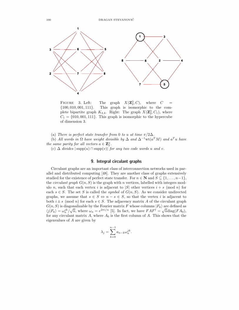
100 DRAGAN STEVANOVIC
Figure 3. Left: The graph X(Z32, C), where C =
{100, 010, 001, 111}. This graph is isomorphic to the com-plete bipartite graph K4,4. Right: The graph X(Z3
2, C1), whereC1 = {010, 001, 111}. This graph is isomorphic to the hypercubeof dimension 3.
(a) There is perfect state transfer from 0 to u at time π/2Δ.(b) All words in Ω have weight divisible by Δ and Δ−1wt(aTM) and aTu have
the same parity for all vectors a ∈ Zn2 .
(c) Δ divides | supp(u) ∩ supp(v)| for any two code words u and v.
9. Integral circulant graphs
Circulant graphs are an important class of interconnection networks used in par-allel and distributed computing [48]. They are another class of graphs extensivelystudied for the existence of perfect state transfer. For n ∈ N and S ⊆ {1, . . . , n−1},the circulant graph G(n, S) is the graph with n vertices, labelled with integers mod-ulo n, such that each vertex i is adjacent to |S| other vertices i + s (mod n) foreach s ∈ S. The set S is called the symbol of G(n, S). As we consider undirectedgraphs, we assume that s ∈ S ⇔ n − s ∈ S, so that the vertex i is adjacent toboth i± s (mod n) for each s ∈ S. The adjacency matrix A of the circulant graphG(n, S) is diagonalizable by the Fourier matrix F whose columns |Fk〉 are defined as〈j|Fk〉 = ωjk
n /√n, where ωn = e2πi/n [5]. In fact, we have FAF † =
√ndiag(FA0),
for any circulant matrix A, where A0 is the first column of A. This shows that theeigenvalues of A are given by
λj =
n−1∑
k=0
an−kωjkn .

APPLICATIONS OF GRAPH SPECTRA IN QUANTUM PHYSICS 101
So [81] has characterized the integral circulant graphs. Let
Gn(d) = {k : gcd(n, k) = d, 1 � k < n}be a set of all integers less than n having the same greatest common divisor d withn. In particular, |Gn(d)| = φ(n/d), where
φ(m) = |{s : gcd(m, s) = 1, 1 � s < m}denotes the Euler phi-function. Let Dn be a set of positive divisors d of n, withd � n/2.
Theorem 9.1. [81] A circulant graph G(n, S) is integral if and only if
S =⋃
d∈D
Gn(d)
for some set of divisors D ⊆ Dn.
Actually, integral circulants were characterized long before by Bridges and Menain 1979 [16], they also extended their result to Cayley graphs of abelian groups in1982 [17].
For a set of divisors D = {d1, . . . , dk} ⊆ Dn, we shortly denote by ICGn(D)
an integral circulant graph G(n,⋃k
i=1Gn(di)). ICGn(D) is connected if and only
gcd(n, d1, . . . , dk) = 1 [81].It was shown in [10] that perfect state transfer is possible in ICGn(D) for even n
only, in which case perfect state transfer exists between antipodal vertices a anda+ n/2, for each a.
The integral circulants with D = {1} are also called the unitary Cayley graphs.
Theorem 9.2. [10] The only unitary Cayley graphs ICGn({1}) with perfect statetransfer are P2 and C4
∼= P⊗22 .
The cocktail-party graph, which is a complete graph Kn minus a perfect match-ing, has perfect state transfer between antipodal vertices at distance two [86]. It isanother example of an integral circulant graph with S = {1, . . . , n− 1}� {n/2}.
Among other integral circulant graphs (non-unitary and non-cocktail-party),the smallest graphs with perfect state transfer are ICG8({1, 2}) and ICG8({1, 4}),shown in Fig. 4. They represent two infinite families of integral circulants withperfect state transfer.
Theorem 9.3. [8] For n divisible by 8, the integral circulant graphs ICGn({1, n/2})and ICGn({1, n/4}) have perfect state transfer between antipodal vertices.
Further examples of integral circulants with perfect state transfer have beenfound in [5], using the concept of circulant join. For a n-vertex graph G and an× n (0, 1)-matrix C, the circulant join G�C G is a graph with adjacency matrix
AG�CG =
[AG CC AG
].
This operation generalizes the usual join G�G = G�J G and K2 +G = G�I G.If u is a vertex of G, then we denote by (u, s), s ∈ {0, 1}, the vertex u in the s-thcopy of G in G�C G.

102 DRAGAN STEVANOVIC
Figure 4. The integral circulant graphs ICG8({1, 2}) and ICG8({1, 4}).
Theorem 9.4. [5] Let C be a n× n circulant matrix. If G is a n-vertex circulantgraph with perfect state transfer from a to b at time t∗, then the circulant joinG�C G has perfect state transfer from vertex (a, 0) to vertex (b, s), s ∈ {0, 1}, attime t∗ provided that
[cos(t∗√B)]1−s [
sin(t∗√B)B−1/2CT
]s= ±I
where B = CTC and B−1 exists whenever s = 1. Also, G�CG is a circulant graphif C is a palindrome circulant matrix, where cj = cn−1−j, for j = 0, 1, . . . , n− 1.
Corollary 9.1. [5] If G is a n-vertex circulant graph that has perfect state transferfrom a to b at time t∗, then so does the circulant graph G�G provided nt∗ ∈ 2πZ.
Theorem 9.5. [5] Let n = 2um, where u � 3 and m � 3 is an odd number.Suppose that G = ICGn(D), for D = {1, n/4} or D = {1, n/2}. For any subsetQ ⊂ Dm ∪ {m}, there is an (0, 1)-circulant matrix C /∈ {In, Jn, On} so that
G�C G = ICG2n(2D ∪Q)
has perfect state transfer from 0 to n/2 in G at time t∗ = π/2.
Corollary 9.2. [5] For n = 2u, for u � 3, the integral circulants ICG2n({1, 2, n/2})and ICG2n({1, 2, n}) have perfect state transfer from 0 to n at time t∗ = π/2.
Still, the integral circulants with perfect state transfer exhibit very small com-munication distance, as their diameter is of order O(ln lnn) [84], inferior to thecommunication distance 2 log3 n found in a P3-cube [27].
Besides few examples of perfect state transfer above, one can actually find moreresults in the literature on the nonexistence of perfect state transfer in integralcirculants:
Theorem 9.6. An integral circulant graph ICGn(D) does not have perfect statetransfer if any of the following conditions hold:

APPLICATIONS OF GRAPH SPECTRA IN QUANTUM PHYSICS 103
(i) n is odd [76];(ii) n/d is odd for every d ∈ D [10];(iii) n is an even square-free integer [8];(iv) n = 2p2 for a prime number p [9].(v) n is not square-free, D �= {1, n/2}, there exists an isolated divisor d0 ∈ D
such that gcd(d0, d) = 1 for every d ∈ D� {d0} and n/d0 is square-free [9];(vi) n ∈ 4N+ 2 and n/d is not square-free for each divisor d ∈ D [9];
10. Other graph compositions
Angeles-Canul et al. [5] and Ge et al. [37] have considered a number of graphcompositions which yield graphs with perfect state transfer under suitable con-ditions. Here we review the results on perfect state transfer in direct product,generalized lexicographic product and join of graphs.
The direct product G×H is a graph defined on V (G) × V (H) where (g1, h1) isadjacent to (g2, h2) if (g1, g2) ∈ E(G) and (h1, h2) ∈ EH . The adjacency matrix ofG×H is AG ⊗AH .
Theorem 10.1. [37] Let G be a graph with perfect state transfer at time tG so that
tG Spec(G) ⊂ Zπ.
Then G×H has perfect state transfer if H is a circulant graph with odd eigenvalues.
Note that Q2n has eigenvalues λk = 2n − 2k, for k = 0, 1, . . . , 2n and perfectstate transfer time t = π/2. Also, P⊗n
3 has eigenvalues from λk ∈ Z√2 and perfect
state transfer time t = π/√2. In both cases, we have tλk ∈ Zπ for all k. Thus,
Q2n × H and P⊗n3 × H have perfect state transfer for any circulant H with odd
eigenvalues. For example, we may let H = Km be the complete graph of order m,for an even integer m.
The generalized lexicographic product GC [H ] of graphs G and H , under thesquare (0, 1)-matrix C indexed by vertices of H , is a graph on VG × VH where(g1, h1) is adjacent to (g2, h2) if and only if either (g1, g2) ∈ EG and C(h1, h2) = 1,or, g1 = g2 and (h1, h2) ∈ EH . The adjacency matrix of GC [H ] is AGC [H] =AG ⊗ AC + IG ⊗ AH . The standard lexicographic product G[H ] is obtained bysetting C = JH .
Theorem 10.2. [37] Let G and H be perfect state transfer graphs with a commontime t, with H being a circulant graph. Suppose that
t|VH | Spec(G) ⊂ 2πZ.
Then the lexicographic product GJH−IH [H ] has perfect state transfer at time t.
Theorem 10.3. [37] Let G be an arbitrary graph and let H be a regular graph withperfect state transfer at time tH from h1 to h2, for h1, h2 ∈ VH . Then G[H ] hasperfect state transfer from (g, h1) to (g, h2) for any g ∈ VG, if
tH |VH | Spec(G) ⊂ 2πZ.

104 DRAGAN STEVANOVIC
Figure 5. Double cones K2 � C8 and K2 � C8.
Corollary 10.1. [37] Suppose H is a kH -regular graph with perfect state transferat time tH = π
2 kH and G is an integral graph. Then G[H ] has perfect state transferprovided kH |VH | Spec(G) ⊂ 4Z.
The n-cubeQn is a n-regular graph on 2n vertices which has perfect state transferat time nπ
2 . Thus, for any integral graph G, the composition graph G[Qn] hasperfect state transfer if n � 2.
The join G�H is a graph defined on V (G)∪ V (H) obtained by taking disjointcopies of G and H and by connecting all vertices of G to all vertices of H . Theadjacency matrix of G�H is
[AG JJ AH
]. The cone of a graph G is defined as K1�G.
The double cone of G is K2 �G, whereas the connected double cone is K2 �G.Bose et al. [15] observed that, althoughKn does not exhibit perfect state transfer,
perfect state transfer is created between any two of its vertices by removing an edgebetween them. Note that this graph is the double cone K2 �Kn−2.
The existence of perfect state transfer in a join of two arbitrary regular graphsmay be reduced to the existence of perfect state transfer in one of the graphsalong with certain structure-independent constraints on the sizes and degrees ofthe graphs.
Theorem 10.4. [5] Let G be a m-vertex kG-regular graph and let H be an n-vertexkH-regular graph. Let a and b be two vertices in G. Then
〈b|e−iAG�Ht|a〉 = 〈b|e−iAGt|a〉+ e−ikGt
m
{eitδ/2
[cos(Δt
2
)− i( δΔ
)sin(Δt
2
)]− 1}
where δ = kG − kH and Δ =√δ2 + 4mn.
This theorem may be applied to the double cones K2 � G and K2 � G. For aprime p, let Sp(n) denote the largest non-negative integer j so that pj |n.Corollary 10.2. [5] For any k-regular graph G on n vertices, K2 �G has perfect
state transfer between the two non-adjacent vertices of K2 if Δ =√k2 + 8n is an
integer and k,Δ ≡ 0 (mod 4) with S2(k) �= S2(Δ).
This corollary may be used to answer a question of Godsil [39, Section 10, ques-tion (b)]: for l � 2, the double-cone graphs K2� (C2(2l−1)+C2l+1) are nonperiodicand have perfect state transfer. They have mixture of integral and irrational eigen-values, so they violate the eigenvalue ratio condition, and hence cannot be periodic.

APPLICATIONS OF GRAPH SPECTRA IN QUANTUM PHYSICS 105
Corollary 10.3. [5] For any k-regular graph G on n vertices, K2 �G has perfect
state transfer between the two adjacent vertices of K2 if Δ =√(k − 1)2 + 8n is an
integer and k − 1,Δ ≡ 0 (mod 8).
11. Perfect routing of quantum states
The transfer of quantum states was introduced as a protocol to simplify interac-tion between distant qubits in a quantum architecture that has locality restrictions,as in solid state systems [71]. The perfect transfer protocols are designed to trans-fer a quantum state which is input on a given site, onto a specific, correspondingoutput site. Although it is desirable to assume no interaction with the system, andjust let its (fixed) Hamiltonian generate the state transfer, this assumption does notuse a vital element of the state transfer protocol—it is implicitly assumed that oneis able to introduce the quantum state onto the input node, and remove it from theoutput node, quickly in comparison to the Hamiltonian dynamics. This additionallevel of control enables several new features, as recently observed in [72].
We start by considering a one-dimensional system of 3N +1 qubits, as depictedin Fig. 6(a), in order to illustrate the basic idea of the construction. The fixed XYHamiltonian takes the form
H =1
2
∑
{i,j}∈E
Ji,j(σxi σ
xj + σy
i σyj )
where E is the set of edges of the graph depicted in Fig. 6(a) and Ji,j = 1 unless{i, j} = {3k, 3k+1} for some k, in which case Ji,j = −1. Same as in Section 3, theHamiltonian is spin preserving,
[H,
3N+1∑
i=1
σzi
]= 0,
and we assume that all spins are initialised in the |0〉 state. By introducing thestate to be transferred on a particular spin, the system is placed in a superpo-sition of 0 and 1 excitations. The 0 excitation subspace is a single state, whichis invariant under the Hamiltonian evolution, and we concentrate on the singleexcitation subspace. The basis states in this subspace are denoted by |n〉 =|0〉⊗n−1|1〉|0〉⊗3N+1−n.
The crucial observation is that, for example, (|2〉 + |3〉)/2 is a 0 eigenstate for(σx
2σx4 + σy
2σy4 ) − (σx
3σx4 + σy
3σy4 ), and similarly, (|2〉 − |3〉)/2 is a 0 eigenstate for
(σx1σ
x2 + σy
1σy2 ) + (σx
1σx3 + σy
1σy3 ). This means that one can rewrite the basis states
as |λ3n+1〉 = |3n + 1〉, |λ3n+2〉 = (|3n + 2〉 + |3n + 3〉)/2, and |λ3n+3〉 = (|3n +2〉−|3n+3〉)/2, leaving the Hamiltonian with a direct sum structure as depicted inFig. 6(b). Each subsystem is now a uniformly coupled path of length 2 or 3, which
achieves perfect transfer in time π/√2 or π/2, respectively.
Thus, starting with a state |λ3n〉, after a time π/2, we obtain |λ3n+2〉 fromHamiltonian dynamics. Now, observe that a fast application of the local rotations
(but globally applied) U =∏N
i=1 σz3n converts between states |λ3n+2〉 and |λ3n+3〉,
i.e., it transfers the state from one subsystem to the next. Hence, starting from

106 DRAGAN STEVANOVIC
Figure 6. (a) A quasi-one-dimensional routing structure. Thecircles represent qubits, and the lines indicate a coupling betweenpairs of qubits of strength +1, unless −1 is indicated. (b) Undera basis transformation, a simple direct sum structure is apparent.In this case, all coupling strengths are equal to
√2.
|λ3n+2〉, we apply U every π/2 and after |m−n|π/2, we get the state |λ3m+2〉. Thisachieves the long range transfer, and a few further details given in [71] are neededto show how to convert from the input state, either |3n+ 1〉 or |3n+ 2〉 to |λ3n+2〉and back to the output state, with the help of the local magnetic fields.
Thus, we can perfectly propagate a quantum state along the length of the sys-tem, between any two vertices in a time proportional to the distance between them.Since the subsystems in Fig. 6(b) are independent, we can actually have multipleexcitations in the system provided they are each separated by at least one sub-system. Thus, multiple states can be transferred at once, enabling a transfer ratewhich is in excess of that achievable in perfect state transfer schemes. These re-sults are easily generalized to two and more dimensions, yielding networks whichcan perfectly route quantum states from arbitrary vertices in a time linear in thedistance to be covered.
Perfect routing of quantum states has also been studied in [30], where it isshown that multiple vertices can faithfully send entanglement through the oscillatorhypercube network at the same time.
12. Conclusion
Due to the bound in the total length of this article, we have surveyed herethe perfect state transfer in uniformly coupled spin networks (simple graphs) only.When one allows non-uniform couplings in the network, such as in the previoussection on routing of quantum states, then it is possible, for example, to engineerthe couplings such that an arbitrarily long path enables the perfect state transferbetween its ends, leading to the notion of quantum wires [27].
Another aspect of perfect state transfer that we did not consider here is itsphysical implementation. There is a large body of physics literature on this topic,and most of it is listed in references below, so that the interested researcher may findit as a useful start point. The technique of perfect routing of quantum states [30,

APPLICATIONS OF GRAPH SPECTRA IN QUANTUM PHYSICS 107
71, 72] appears to be especially promising in bringing the quantum state transfercloser to its physical realization.
The problem of the maximum communication distance is very much untouched.The largest known communication distance of 2 log3 n was achieved already for one
of the very first perfect state transfer networks, the Cartesian product P⊗d3 of three-
vertex paths [28]. The integral circulants, due to their extremely small diameterO(log logn), are unable to provide larger communication distances. The situationis similar with other constructions, which in some cases cannot perform better thanto achieve perfect state transfer between vertices at a small constant distance (2or 3). Thus, it is a main open problem to see whether a larger communicationdistance, for example, of order O(
√n), may be achieved.
Among graph compositions, most elegant connection to the perfect state transferis exhibited by the Cartesian product of graphs, which is a particular case of NEPS.Bernasconi et al. [13] have, with a single unresolved case, managed to characterizeperfect state transfer in cubelike graphs, which itself is NEPS of P2s. Thus, thenext interesting question is to find out whether similar conditions will enable perfectstate transfer in NEPS of P3s.
Acknowledgement. The author is grateful to Chris Godsil for constructive com-ments on the first draft of this survey, and also to Matthew Russell for makingavailable his example of nonperiodic regular graph with perfect state transfer.
References
[1] D. Aerts, T. Durt, M. Czachor, Probing the structure of quantum mechanics: Nonlinearity,Nonlocality, Computation and Axiomatics, World Scientific, Brussels, Belgium, 2000.
[2] C. Albanese, M. Christandl, N. Datta, A. Ekert, Mirror Inversion of Quantum States inLinear Registers, Phys. Rev. Lett. 93 (2004) 230502.
[3] G. A. Alvarez, M. Mishkovsky, E.P. Danieli, P. R. Levstein, H.M. Pastawski, L. Frydman,Perfect state transfer by selective quantum interferences within complex spin networks,
arXiv:1005.2593v1 [quant-ph].[4] P.W. Anderson, Absence of diffusion in certain random lattices, Phys. Rev. 109 (1958),
1492–1505.[5] R. J. Angeles-Canul, R. Norton, M. Opperman, C. Paribello, M. Russel, C. Tamon, Perfect
state transfer, integral circulants and join of graphs, Quantum Inf. Comput. 10 (2010),325–342.
[6] R. J. Angeles-Canul, R. Norton, M. Opperman, C. Paribello, M. Russel, C. Tamon, Onquantum perfect state transfer in weighted join graphs, arXiv:0909.0431v1 [quant-ph].
[7] K. Balinska, D.M. Cvetkovic, Z. Radosavljevic, S. Simic, D. Stevanovic, A survey on integralgraphs, Univ. Beograd, Publ. Elektrotehn. Fak, Ser. Mat. 13 (2002), 42–65.
[8] M. Basic, M. Petkovic, Some classes of integral circulant graphs either allowing or notallowing perfect state transfer, Appl. Math. Lett. 22 (2009), 1609–1615.
[9] M. Basic, M. Petkovic, Perfect state transfer in integral circulant graphs of non-square-freeorder, Linear Algebra Appl. 433 (2010), 149–163.
[10] M. Basic, M. Petkovic, D. Stevanovic, Perfect state transfer in integral circulant graphs,Appl. Math. Lett. 22 (2009), 1117–1121.
[11] C. H. Bennett, S. J. Wiesner, Communication via one- and two-particle operators onEinstein-Podolsky-Rosen states, Phys. Rev. Lett. 69 (1992) 2881–2884.
[12] C. H. Bennett, G. Brassard, C. Crepeau, R. Jozsa, A. Peres, W.K. Wooters, Teleportingan unknown quantum state via dual classical and Einstein-Podolsky-Rosen channels, Phys.Rev. Lett. 70 (1993) 1895–1899.

108 DRAGAN STEVANOVIC
[13] A. Bernasconi, C. Godsil, S. Severini, Quantum networks on cubelike graphs, Phys. Rev. A78 (2008), 052320, arXiv:0808.0510v1 [quant-ph].
[14] S. Bose, Quantum Communication through an Unmodulated Spin Chain, Phys. Rev. Lett.91 (2003) 207901.
[15] S. Bose, A. Casaccino, S. Mancini, S. Severini, Communication in XY Z all-to-all quantumnetworks with a missing link, Int. J. Quantum Inf. 7 (2009), 713–723.
[16] W.G. Bridges, R.A. Mena, Rational circulants with rational spectra and cyclic stronglyregular graphs, Ars Comb. 8 (1979), 143–161.
[17] W.G. Bridges, R.A. Mena, Rational G-matrices with rational eigenvalues, J. Comb. Theory,Ser. A 32 (1982), 264–280.
[18] D. Burgarth, S. Bose, Conclusive and arbitrarily perfect quantum-state transfer using par-allel spin-chain channels, Phys. Rev. A 71 (2005) 052315.
[19] D. Burgarth, S. Bose, Perfect quantum state transfer with randomly coupled quantumchains, New J. Phys 7 (2005) 135.
[20] D. Burgarth, V. Giovannetti, S. Bose, Efficient and perfect state transfer in quantum chains,J. Phys. A: Math. Gen. 38 (2005) 6793–6802.
[21] F. C. Bussemaker, D. Cvetkovic, There are exactly 13 connected, cubic, integral graphs,Univ. Beograd, Publ. Elektrotehn. Fak, Ser. Mat. Fiz 544/576 (1976), 43–48.
[22] A. Casaccino, S. Lloyd, S. Mancini, S. Severini, Quantum state transfer through a qubitnetwork with energy shifts and fluctuations, arXiv:0904.4510v1 [quant-ph].
[23] J. L. Chen, Q. L. Wang, Perfect Transfer of Entangled States on Spin Chain, Int. J. Theor.Phys. 46 (2007) 614–624.
[24] W.C. Cheung, C. Godsil, Perfect State Transfer in Cubelike Graphs, arXiv:1010.4721v1[math.CO].
[25] A. Childs, E. Farhi, S. Gutmann, An Example of the Difference Between Quantum andClassical Random Walks, Quantum Inf. Process. 1 (2002) 35–43.
[26] A. Childs, Universal quantum computation by quantum walk, Phys. Rev. Lett. 102 (2009),180501.
[27] M. Christandl, N. Datta, T. C. Dorlas, A. Ekert, A. Kay, A. J. Landahl, Perfect transfer ofarbitrary states in quantum spin networks, Phys. Rev. A 71 (2005), 032312.
[28] M. Christandl, N. Datta, A. Ekert, A. J. Landahl, Perfect State Transfer in Quantum SpinNetworks, Phys. Rev. Lett. 92 (2004) 187902.
[29] M.T. Chu, G.H. Golub, Structured inverse eigenvalue problems, Acta Numerica 11 (2002),1–71.
[30] C. Chudzicki, F.W. Strauch, Parallel State Transfer and Efficient Quantum Routing onQuantum Networks, arXiv:1008.1806v1 [quant-ph].
[31] D. Cvetkovic, M. Doob, H. Sachs, Spectra of Graphs—Theory and Application, AcademicPress, New York, 1979.
[32] D. Cvetkovic, P. Rowlinson, S. Simic, Eigenspaces of Graphs, Cambridge University Press,Cambridge, 1997.
[33] D. Cvetkovic, P. Rowlinson, S. Simic, An Introduction to the Theory of Graph Spectra,Cambridge University Press, Cambridge, 2009.
[34] C. Di Franco, M. Paternostro, M. S. Kim, Perfect State Transfer on a Spin Chain withoutState Initialization, Phys. Rev. Lett. 101 (2008) 230502.
[35] E. Farhi, S. Gutmann, Quantum computation and decision trees, Phys. Rev. A 58 (1998)915–928.
[36] D. L. Feder, Perfect Quantum State Transfer with Spinor Bosons on Weighted Graphs,Phys. Rev. Lett. 97 (2006) 180502.
[37] Y. Ge, B. Greenberg, O. Perez, C. Tamon, Perfect state transfer, graph products and equi-table partitions, arXiv:1009.1340v1 [quant-ph].
[38] N. Gisin, G. Ribordy, W. Tittel, H. Zbinden, Quantum cryptography, Rev. Mod. Phys. 74(2002) 145–195.
[39] C. Godsil, Periodic Graphs, arXiv:0806.2074v2 [math.CO].

APPLICATIONS OF GRAPH SPECTRA IN QUANTUM PHYSICS 109
[40] C. Godsil, When can perfect state transfer occur?, preprint.[41] C. Godsil, Algebraic Combinatorics, Chapman and Hall, 1993.[42] J. Gong, P. Brumer, Controlled quantum-state transfer in a spin chain, Phys. Rev. A 75
(2007) 032331.[43] G. Gualdi, V. Kostak, I. Marzoli, P. Tombesi, Perfect state transfer in long-range interacting
spin chains, Phys. Rev. A 78 (2008) 022325.[44] G. Gualdi, I. Marzoli, P. Tombesi, Entanglement generation and perfect state transfer in
ferromagnetic qubit chains, New J. Phys 11 (2009) 063038.[45] G. R. Guthorlein, M. Keller, K. Hayasaka, W. Lange, H. Walther, A single ion as a
nanoscopic probe of an optical field, Nature (London) 414 (2001) 49–51.[46] M. J. Hartmann, M.E. Reuter, M.B. Plenio, Excitation and entanglement transfer versus
spectral gap, New J. Phys 8 (2006) 94.[47] J. He, Q. Chen, L. Ding, S.-L. Wan, Conclusive and perfect quantum state transfer with a
single spin chain, Phys. Lett. A 372 (2008) 185–190.[48] F. K. Hwang, A survey on multi-loop networks, Theor. Comput. Sci. 299 (2003), 107–121.[49] M.A. Jafarizadeh, R. Sufiani, Perfect state transfer over distance-regular spin networks,
Phys. Rev. A 77 (2008), 022315.[50] M.A. Jafarizadeh, R. Sufiani, M. Azimi, F. Eghbali Fam, Perfect state transfer over inter-
acting boson networks associated with group schemes, arXiv:1007.2106v1 [quant-ph].[51] M.A. Jafarizadeh, R. Sufiani, S. F. Taghavi, E. Barati, Optimal transfer of a d-level quantum
state over pseudo-distance-regular networks. J. Phys. A: Math. Theor. 41 (2008) 475302.[52] M.A. Jafarizadeh, R. Sufiani, S. F. Taghavi, E. Barati, Perfect transfer of m-qubit GHZ
states, arXiv:0805.1866v1 [quant-ph].[53] G. James, M. Liebeck, Representations and characters of groups, Cambridge University
Press, Cambridge, 1993.[54] B. E. Kane, A silicon-based nuclear spin quantum computer, Nature (London) 393 (2003)
133–137.[55] P. Karbach, J. Stolze, Spin chains as perfect quantum state mirrors, Phys. Rev. A 72 (2005)
030301.[56] A. Kay, Perfect state transfer: Beyond nearest-neighbor couplings, Phys. Rev. A 73 (2006)
032306.[57] A. Kay, A Review of Perfect, Efficient, State Transfer and its Application as a Constructive
Tool, arXiv:0903.4274v3 [quant-ph].[58] A. Kay, Unifying Quantum State Transfer and State Amplification, Phys. Rev. Lett. 98
(2007) 010501.[59] A. Kay, The Topological Properties of Fault-Tolerant Circuits, arXiv:quant-ph/0702092v3.
[60] A. Kay, M. Ericsson, Geometric effects and computation in spin networks, New J. Phys 7(2005) 143.
[61] T. Kimura, Y. Nambu, T. Hatanaka, A. Tomita, H. Kosaka, K. Nakamura, Single-photonInterference over 150km Transmission Using Silica-based Integrated-optic Interferometersfor Quantum Cryptography, Jpn. J. Appl. Phys, Part 2, 43 (2004), L1217–L1219.
[62] V. Kostak, G.M. Nikolopoulos, I. Jex, Perfect state transfer in networks of arbitrary topol-ogy and coupling configuration, Phys. Rev. A 75 (2007), 042319.
[63] D. Leibfried, B. Demarco, V. Meyer, D. Lucas, M. Barrett, J. Britton, W.M. Itano, B.Jelenkovic, C. Langer, T. Rosenblad, D. J. Wineland, Experimental demonstration of arobust, high-fidelity geometric two ion-qubit phase gate, Nature (London) 422 (2003) 412–415.
[64] D. Loss, D.P. DiVincenzo, Quantum computation with quantum dots, Phys. Rev. A 57(1998) 120–126.
[65] O. Mandel, M. Greiner, A. Widera, T. Rom, T.W. Hansch, I. Bloch, Controlled collisionsfor multi-particle entanglement of optically trapped atoms, Nature (London) 425 (2003)937.

110 DRAGAN STEVANOVIC
[66] M. Markiewicz, M. Wiesniak, Perfect state transfer without state initialization and remotecollaboration, Phys. Rev. A 79 (2009) 054304.
[67] C. Moore, A. Russell, Quantum Walks on the Hypercube, in Proc. 6th Int. Workshop onRandomization and Approximation in Computer Science, Lect. Notes Comput. Sci. 2483(2002) 164–178, Springer.
[68] M. Mosca, Quantum Algorithms, Springer Encyclopedia of Complexity and Systems Science,Springer, New York, 2009, arXiv: 0808.0369v1 [quant-ph].
[69] G.M. Nikolopoulos, D. Petrosyan, P. Lambropoulos, Coherent electron wavepacket prop-agation and entanglement in array of coupled quantum dots, Europhys. Lett. 65 (2004),297–303.
[70] I.M. Niven, Irrational numbers, Mathematical Association of America, New York, 1956.[71] P. J. Pemberton-Ross, A. Kay, Perfect Quantum Routing in Regular Spin Networks,
arXiv:1007.2786v2 [quant-ph].[72] P. J. Pemberton-Ross, A. Kay, S. G. Schirmer, Quantum Control Theory for State Trans-
formations: Dark States and their Enlightenment, arXiv:1003.4290 [quant-ph].[73] O. Romero-Isart, K. Eckert, A. Sanpera, Quantum state transfer in spin-1 chains, Phys.
Rev. A 75 (2007) 050303(R).[74] J. Rosser, L. Schoenfeld, Approximate formulas for some functions of prime numbers, Ill.
J. Math. 6 (1962) 64–94.[75] M. Russell, A non-integral regular graph with perfect state transfer, preprint.[76] N. Saxena, S. Severini, I. Shparlinski, Parameters of integral circulant graphs and periodic
quantum dynamics, Int. J. Quantum Inf. 5 (2007), 417–430.[77] F. Schmidt-Kaler, H. Haffner, M. Riebe, S. Gulde, G. P.T. Lancaster, T. Deuschle, C.
Becher, C. F. Roos, J. Eschner, R. Blatt, Realization of the Cirac-Zoller controlled-NOTquantum gate, Nature (London) 422 (2003) 408–411.
[78] A. J. Schwenk, Exactly thirteen connected cubic graphs have integral spectra, in: Y. Alavi,D. Lick (eds.), Proceedings of the International Graph Theory Conference at Kalamazoo,May 1976, Lect. Notes Math. 642, Springer-Verlag, Berlin, 1978, 516–533.
[79] S. Severini, The 3-dimensional cube is the only connected cubic graph with perfect statetransfer, arXiv:1001.0674v2 [quant-ph].
[80] T. Shi, Y. Li, Z. Song, C.P. Sun, Quantum-state transfer via the ferromagnetic chain in aspatially modulated field, Phys. Rev. A 71 (2005) 032309.
[81] W. So, Integral circulant graphs, Discrete Math. 306 (2006), 153–158.[82] D. Stevanovic, 4-Regular integral graphs avoiding ±3 in the spectrum, Univ. Beograd, Publ.
Elektrotehn. Fak, Ser. Mat. 14 (2003), 99–110.[83] D. Stevanovic, N.M.M. de Abreu, M.A.A. de Freitas, R. Del-Vecchio, Walks and Regular
Integral Graphs, Linear Algebra Appl. 423 (2007), 119–135.[84] D. Stevanovic, M. Petkovic, M. Basic, On the diameter of integral circulant graphs, Ars
Combinatoria, in press.[85] F.W. Strauch, C. J. Williams, Theoretical analysis of perfect quantum state transfer with
superconducting qubits, Phys. Rev. B 78 (2008) 094516.[86] D. I. Tsomokos, M.B. Plenio, I. de Vega, S. F. Huelga, State transfer in highly connected
networks and a quantum Babinet principle, Phys. Rev. A 78 (2008) 062310.[87] M. S. Underwood, D. L. Feder, Universal quantum computation by discontinuous quantum
walk, arXiv:1008.3578v1 [quant-ph].[88] A.Y. Vlasov, Programmable quantum state transfer, arXiv:0708.0145v2 [quant-ph].[89] L. Wang, A survey of results on integral trees and integral graphs, University of Twente,
Electrical Engineering, Mathematics and Computer Science, Internal Report, 2005, http://doc.utwente.nl/65947/.
[90] Wikipedia, Hamiltonian (quantum mechanics), http://en.wikipedia.org/wiki/Hamiltonian(quantum\ mechanics).
[91] Wikipedia, Mathematical formulations of quantum mechanics, http://en.wikipedia.org/wiki/Mathematical formulations of quantum mechanics.
APPLICATIONS OF GRAPH SPECTRA IN QUANTUM PHYSICS 111
[92] Wikipedia, List of mathematical topics in quantum theory, http://en.wikipedia.org/wiki/List\ of\ mathematical\ topics\ in\ quantum\ theory.
[93] Wikipedia, Symplectic manifold, http://en.wikipedia.org/wiki/Symplectic\ manifold.[94] Wikipedia, Quantum computing, http://en.wikipedia.org/wiki/Quantum\ computing.[95] Wikipedia, Qubit, http://en.wikipedia.org/wiki/Qubit.[96] X.Q. Xi, J. B. Gong, T. Zhang, R. H. Yue, W.M. Liu, Explicit designs of spin chains for
perfect quantum state transfer, Eur. Phys. J. D 50 (2008), 193–199.[97] S. Yang, Z. Song, C.P. Sun, Quantum state swapping via a qubit network with Hubbard
interactions, Phys. Rev. B 73 (2008) 195122.[98] L. Ying, S. Zhi, S. Chang-Pu, Perfect Transfer of Many-Particle Quantum State via High-
Dimensional Systems with Spectrum-Matched Symmetry, Commun. Theor. Phys. (Beijing,China) 48 (2007), 445–448.
[99] Z.-S. Yuan, X.-H. Bao, C.-Y. Lu, J. Zhang, C.-Z. Peng, J.-W. Pan, Entangled photons andquantum communication, Phys. Rep. (2010), doi:10.1016/j.physrep.2010.07.004
[100] M.-H. Yung, S. Bose, Perfect state transfer, effective gates, and entanglement generationin engineered bosonic and fermionic networks, Phys. Rev. A 71 (2005) 032310.
[101] J. Zhang, G. L. Long, W. Zhang, Z. Deng, W. Liu, Z. Lu, Simulation of Heisenberg XYinteractions and realization of a perfect state transfer in spin chains using liquid nuclearmagnetic resonance, Phys. Rev. A 72 (2005) 012331.


Ivan Gutman
HYPERENERGETIC ANDHYPOENERGETIC GRAPHS
Abstract. The energy E = E(G) of a graph G is the sum of theabsolute values of the eigenvalues of G. The motivation for the in-troduction of this invariant comes from chemistry, where results onE were obtained already in the 1940’s. A graph G with n vertices issaid to be “hyperenergetic” if E > 2n− 2, and to be “hypoenergetic”if E(G) < n. In this chapter we outline the main hitherto obtainedresults related to hyperenergetic and hypoenergetic graph.
Mathematics Subject Classification (2010): 05C50; 05C90; 92E10
Keywords : energy (of graph); hyperenergetic graph; hypoenergeticgraph; spectrum (of graph); chemistry

Contents
1. Energy of a graph 1142. The chemical connection 1153. Hyperenergetic graphs 1194. Hypoenergetic graphs 1205. Interlude: biregular and triregular graphs 1236. A lower bound for energy and its applications 1247. On the energy of biregular graphs 1257.1. Biregular trees 1257.2. Unicyclic biregular graphs 1267.3. Bicyclic biregular graphs 127References 132
1. Energy of a graph
Definition 1. Let G be a graph on n vertices and let λ1, λ2, . . . , λn be its eigen-values [7, 11]. Then the energy of G is
(1) E = E(G) =
n∑
j=1
|λj |.
Although in the chemical literature the sum of absolute values of the eigenvaluesof some graphs was (in a more-or-less implicit manner) considered already sincethe 1940s (see e.g., [5, 20, 41, 55, 59]), it was the present author who in the 1970sused Eq. (1) as a definition, noticing that practically all results that until thenwere obtained for the total π-electron energy (cf. the next section), pertain to thequantity occurring on the right–hand side of (1).
Definition 1 was advocated by the present author on several lectures and seminarsheld in the 1970s. In written form it was first stated in the paper [21]. Since thispaper is extremely difficult to acquire, it is not quite surprising that the graph-energy concept was for a long time not recognized by other scholars. The samedefinition was later given in the book [37], and elsewhere [22].
Nowadays, this is history. Its details have been outlined on several occasions[10, 28, 29].
What from the present–day’s point of view is important is the following.First, Eq. (1) does not require (and, in fact: does not permit) a chemical interpre-
tation. Consequently, the graph G needs not satisfy any of the several chemistry-based conditions, such as that it must be connected, that its maximum vertexdegree must not exceed 3, etc. [37]. The graph energy is defined for all graphs andmathematicians may study it without being restricted by any chemistry-causedlimitation.
Second, somewhere around the turn of the century mathematicians realized themathematical value (and, let us say: mathematical beauty) of graph energy, and

HYPERENERGETIC AND HYPOENERGETIC GRAPHS 115
a vigorous and world-wide mathematical research of E started. The current activ-ities on the mathematical studies of E are remarkable: According to our records,in the year 2006 the number of published papers was 11. In 2007, 2008, and 2009this number increased to 30, 47, and 59, respectively. In the time of completionof this chapter (August 2010) the author is aware of 54 papers on graph energypublished in 2010 or in press. Solely in the 21-th century several hundreds ofmathematicians from Australia, Austria, Brazil, Canada, Chile, China, Croatia,Germany, India, Iran, Ireland, Italy, Mexico, Netherlands, Pakistan, Portugal, Ru-mania, Russia, Serbia, South Africa, South Korea, Spain, Sweden, Turkey, UK,USA, and Venezuela participated or are participating in research on graph energy.
Details of the (mathematical) theory of graph energy can be found in the reviews[26, 29, 35, 54] and in the references cited therein. In this chapter we are goingto outline only two aspects of this theory, namely the results pertaining to theconditions E > 2n− 2 and E(G) < n. Before doing this, in the subsequent sectionwe briefly repeat the details on E related to chemistry.
2. The chemical connection
Researches related to the energy of a graph can be traced back to the 1940s oreven to the 1930s. In the 1930s the German scholar Erich Huckel put forward amethod for finding approximate solutions of the Schrodinger equation of a class oforganic molecules, the so-called “unsaturated conjugated hydrocarbons”. Detailsof this approach, often referred to as the “Huckel molecular orbital (HMO) theory”can be found in appropriate textbooks [6, 62, 66].
The Schrodinger equation (or, more precisely: the time-independent Schrodingerequation) is a second-order partial differential equation of of the form
(2) H Ψ = E Ψ
where Ψ is the so-called wave function of the system considered, H the so-calledHamiltonian operator of the system considered, and E the energy of the systemconsidered. When applied to a particular molecule, the Schrodinger equation en-ables one to describe the behavior of the electrons in this molecule and to establishtheir energies. For this one needs to solve Eq. (2), which evidently is an eigenvalue–eigenvector problem of the Hamiltonian operator. In order that the solution of (2)be feasible (yet not completely exact), one needs to express Ψ as a linear combina-tion of a finite number of pertinently chosen basis functions. If so, then Eq. (2) isconverted into:
HΨ = EΨ
where now H is a matrix - the so-called Hamiltonian matrix.The HMO model enables to approximately describe the behavior of the so-called
π-electrons in an unsaturated conjugated molecule, especially of conjugated hydro-carbons. In Fig. 1 is depicted the chemical formula of biphenylene – a typical con-jugated hydrocarbon H . It contains n = 12 carbon atoms over which the n = 12π-electrons form waves.

116 IVAN GUTMAN
C C C
C
C
C
C
CCC
C
CH
H
H
H
H
H
H H
GH
1
1
2
2
3
3
4
4
5
5
6
67
7
8 8
9
910
10
11
11
12
12
Figure 1. Biphenylene H is a typical unsaturated conjugated hy-drocarbon. Its carbon–atom skeleton is represented by the molec-ular graph G. The carbon atoms in the chemical formula H andthe vertices of the graph G are labelled by 1, 2, . . . , 12 so as to bein harmony with Eqs. (3) and (4).
In the HMO model the wave functions of a conjugated hydrocarbon with ncarbon atoms are expanded in an n-dimensional space of orthogonal basis functions,whereas the Hamiltonian matrix is a square matrix of order n, defined so that:
[H]ij =
⎧⎪⎨
⎪⎩
α, if i = j
β, if the atoms i and j are chemically bonded
0, if there is no chemical bond between the atoms i and j.
The parameters α and β are assumed to be constants, equal for all conjugatedmolecules. Their physical nature and numerical value are irrelevant for the presentconsiderations; for details see in [6, 62, 66].
For instance, the HMO Hamiltonian matrix of biphenylene is:
(3) H =
⎡
⎢⎢⎢⎢⎢⎢⎢⎢⎢⎢⎢⎢⎢⎢⎢⎢⎢⎢⎣
α β 0 0 0 β 0 0 0 0 0 0β α β 0 0 0 0 0 0 0 0 β0 β α β 0 0 0 0 0 0 β 00 0 β α β 0 0 0 0 0 β 00 0 0 β α β 0 0 0 0 0 0β 0 0 0 β α 0 0 0 0 0 00 0 0 0 0 0 α β 0 0 0 β0 0 0 0 0 0 β α β 0 0 00 0 0 0 0 0 0 β α β 0 00 0 0 0 0 0 0 0 β α β 00 0 β 0 0 0 0 0 0 β α β0 β 0 0 0 0 β 0 0 0 β α
⎤
⎥⎥⎥⎥⎥⎥⎥⎥⎥⎥⎥⎥⎥⎥⎥⎥⎥⎥⎦
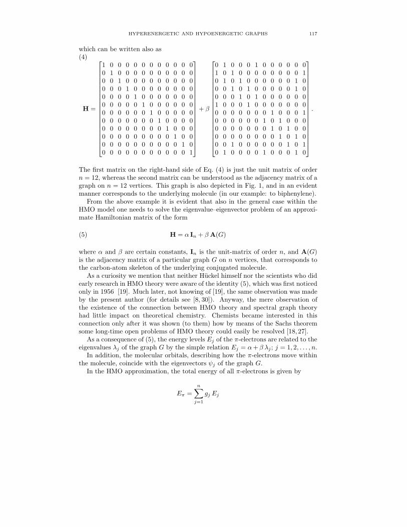
HYPERENERGETIC AND HYPOENERGETIC GRAPHS 117
which can be written also as(4)
H =
⎡
⎢⎢⎢⎢⎢⎢⎢⎢⎢⎢⎢⎢⎢⎢⎢⎢⎢⎢⎣
1 0 0 0 0 0 0 0 0 0 0 00 1 0 0 0 0 0 0 0 0 0 00 0 1 0 0 0 0 0 0 0 0 00 0 0 1 0 0 0 0 0 0 0 00 0 0 0 1 0 0 0 0 0 0 00 0 0 0 0 1 0 0 0 0 0 00 0 0 0 0 0 1 0 0 0 0 00 0 0 0 0 0 0 1 0 0 0 00 0 0 0 0 0 0 0 1 0 0 00 0 0 0 0 0 0 0 0 1 0 00 0 0 0 0 0 0 0 0 0 1 00 0 0 0 0 0 0 0 0 0 0 1
⎤
⎥⎥⎥⎥⎥⎥⎥⎥⎥⎥⎥⎥⎥⎥⎥⎥⎥⎥⎦
+ β
⎡
⎢⎢⎢⎢⎢⎢⎢⎢⎢⎢⎢⎢⎢⎢⎢⎢⎢⎢⎣
0 1 0 0 0 1 0 0 0 0 0 01 0 1 0 0 0 0 0 0 0 0 10 1 0 1 0 0 0 0 0 0 1 00 0 1 0 1 0 0 0 0 0 1 00 0 0 1 0 1 0 0 0 0 0 01 0 0 0 1 0 0 0 0 0 0 00 0 0 0 0 0 0 1 0 0 0 10 0 0 0 0 0 1 0 1 0 0 00 0 0 0 0 0 0 1 0 1 0 00 0 0 0 0 0 0 0 1 0 1 00 0 1 0 0 0 0 0 0 1 0 10 1 0 0 0 0 1 0 0 0 1 0
⎤
⎥⎥⎥⎥⎥⎥⎥⎥⎥⎥⎥⎥⎥⎥⎥⎥⎥⎥⎦
.
The first matrix on the right-hand side of Eq. (4) is just the unit matrix of ordern = 12, whereas the second matrix can be understood as the adjacency matrix of agraph on n = 12 vertices. This graph is also depicted in Fig. 1, and in an evidentmanner corresponds to the underlying molecule (in our example: to biphenylene).
From the above example it is evident that also in the general case within theHMO model one needs to solve the eigenvalue–eigenvector problem of an approxi-mate Hamiltonian matrix of the form
(5) H = α In + βA(G)
where α and β are certain constants, In is the unit-matrix of order n, and A(G)is the adjacency matrix of a particular graph G on n vertices, that corresponds tothe carbon-atom skeleton of the underlying conjugated molecule.
As a curiosity we mention that neither Huckel himself nor the scientists who didearly research in HMO theory were aware of the identity (5), which was first noticedonly in 1956 [19]. Much later, not knowing of [19], the same observation was madeby the present author (for details see [8, 30]). Anyway, the mere observation ofthe existence of the connection between HMO theory and spectral graph theoryhad little impact on theoretical chemistry. Chemists became interested in thisconnection only after it was shown (to them) how by means of the Sachs theoremsome long-time open problems of HMO theory could easily be resolved [18, 27].
As a consequence of (5), the energy levels Ej of the π-electrons are related to theeigenvalues λj of the graph G by the simple relation Ej = α+ β λj ; j = 1, 2, . . . , n.
In addition, the molecular orbitals, describing how the π-electrons move withinthe molecule, coincide with the eigenvectors ψj of the graph G.
In the HMO approximation, the total energy of all π-electrons is given by
Eπ =
n∑
j=1
gj Ej

118 IVAN GUTMAN
where gj is the so-called “occupation number”, the number of π-electrons that movein accordance with the molecular orbital ψj . By a general physical law, gj mayassume only the values 0, 1, or 2.
Details on Eπ and the way in which the molecular graph G is constructed can befound in the books [13,17,37] and reviews [28,29]. There also more information onthe chemical applications of Eπ can be found. For what follows, it is only importantthat because the number of π-electrons in the conjugated hydrocarbon consideredis equal to n, it must be g1 + g2 + · · ·+ gn = n which immediately implies
Eπ = αn+ β
n∑
j=1
gj λj .
In view of the fact that α and β are constants, and that in chemical applications nis also a constant, the only non-trivial part in the above expression is
(6) E =
n∑
j=1
gj λj .
The right-hand side of Eq. (6) is just what in the chemical literature is referred toas “total π-electron energy”; if necessary, then one says “total π-electron energy inβ-units”.
If the π-electron energy levels are labelled in a non-decreasing order: E1 � E2 �· · · � En then the requirement that the total π-electron energy be as low as possibleis achieved if for even n,
gj =
{2, for j = 1, 2, . . . , n/2
0, for j = n/2 + 1, n/2 + 2, . . . , n
whereas for odd n,
gj =
⎧⎪⎨
⎪⎩
2, for j = 1, 2, . . . , (n− 1)/2
1, for j = (n+ 1)/2
0, for j = (n+ 1)/2 + 1, (n+ 1)/2 + 2, . . . , n.
For the majority (but not all!) chemically relevant cases,
gj =
{2, whenever λj > 0
0, whenever λj < 0.
If so, then Eq. (6) becomes: E = E(G) = 2∑
+ λj where∑
+ indicates summationover positive eigenvalues. Because for all graphs, the sum of eigenvalues is equal tozero, we can rewrite the above equality as
(7) E = E(G) =n∑
j=1
|λj |
which by form (but not by “physical meaning”) is identical to Eq. (1).

HYPERENERGETIC AND HYPOENERGETIC GRAPHS 119
3. Hyperenergetic graphs
Definition 2. A graph G on n vertices is said to be hyperenergetic if
E > 2n− 2.
In order to understand the reason for defining “hyperenergeticity” in such aseemingly awkward manner, one needs to recall the following.
In the times when computers were not commonly available, the calculation ofHMO total π-energy (that is, E) was not an easy task. Therefore, much workwas done on finding simple algebraic expressions that would make it possible toobtain an approximate numerical value of E knowing the simple structural detailsof the underlying molecular graph. A particularly successful such approximationwas discovered by McClelland [55], viz.
E ≈ a√2mn
where n andm are the number of vertices (resp., number of carbon atoms) and num-ber of edges (resp., number of carbon–carbon bonds) of the corresponding molec-ular graph (resp., conjugated hydrocarbon), and where a is an empirical constant(a ≈ 0.9). Eventually, scores of other such (n,m)-type approximate expressions forE were designed, whose details can be found in the surveys [23, 39].
Most of the (n,m)-type approximate expressions for E are monotonically in-creasing functions of the parameter m. This, indeed, is in good agreement with theobservedE-values of molecular graphs, which because of the requirement 2m/n � 3,necessarily have small number of edges.
By extrapolating this kind odm-dependence of E, one readily arrives at the con-clusion that among n-vertex graphs, the complete graph Kn would have maximalenergy. Since E(Kn) = 2n− 2, one would thus arrive at:
Conjecture 3.1. [21] If G is an n-vertex graph, G �∼= Kn, then E(G) < 2n− 2.
This conjecture was stated by the present author in his first paper on graphenergy [21]. Soon thereafter, by means of counterexamples, Conjecture 3.1 wasshown to be false [9].
At this point it is worth mentioning that in the 1990s a Chinese mathematician(whose name will be omitted) offered a proof of Conjecture 3.1. He had luck that thepresent author refereed his paper. The error committed in the proof was trivial:a simple quadratic equation was incorrectly solved. This minor mistake impliedthen the expected conclusion that E(G) < 2n− 2. Of course, the paper was neverpublished.
The true work on hyperenergetic graphs started in the late 1990s, independentlyby a group of Indian mathematicians [64] and the present author [25, 36].
Theorem 3.2. [64] (a) For n � 5 the line graph of the complete graph Kn ishyperenergetic.(b) For n � 4 the line graph of the complete bipartite graph Kn,n is hyperenergetic.(c) For n � 6 the line graph of the n-vertex cocktail party graph is hyperenergetic.

120 IVAN GUTMAN
By Theorem 3.2, for the first time, infinitely many hyperenergetic graphs couldbe systematically constructed. Hou and the present author later extended thisresult as follows:
Theorem 3.3. [44] All graphs with more than 2n− 1 edges are hyperenergetic.
In [36] graphs obtained by deleting a few edges from Kn were studied. It wasshown that by deleting one, two, or three edges from Kn, the respective energy issmaller than E(Kn). However, if four edges, forming a quadrangle, are deleted,then the energy exceeds E(Kn). The works [25, 36] implied:
Theorem 3.4. [25] Hyperenergetic graphs on n-vertices exist for all n � 8. Thereare no hyperenergetic graphs on less than 8 vertices.
Eventually, hyperenergeticity was verified for a variety of other classes of graphs:Paley [46], circulant [61], Kneser [2], etc. [3]. For some other graphs, especially thosefor which the maximal vertex degree is 3 or less, it was shown that they cannot behyperenergetic [32, 63].
The mortal blow to the research of hyperenergetic graphs was givew by Nikiforv,who showed:
Theorem 3.5. [56] For almost all graphs
E(G) =
(4
3π+ o(1)
)n3/2.
Theorem 3.5 immediately implies that almost all graphs are hyperenergetic,making any further search for them pointless.
In view of Nikiforov’s negative result, it is interesting that in a recent work [60],Shen at al. proved:
Theorem 3.6. [60] For any c <∞, there exists only a finite number of hyperen-ergetic graphs with cyclomatic number c. In particular, there are no hyperenergeticgraphs with c � 8.
4. Hypoenergetic graphs
Definition 3. A graph G on n vertices is said to be hypoenergetic if
(8) E(G) < n.
Graphs for which
(9) E(G) � n
are said to be non-hypoenergetic.
In the chemical literature it was noticed long time ago that for the vast majorityof (molecular) graphs the energy exceeds the number of vertices. In 1973 thetheoretical chemists England and Ruedenberg published a paper [14] in which theyasked “why is the delocalization energy negative?”. Translated into the language ofgraph spectral theory, their question reads: “why does the graph energy exceed thenumber of vertices?”, understanding that the graph in question is “molecular”.
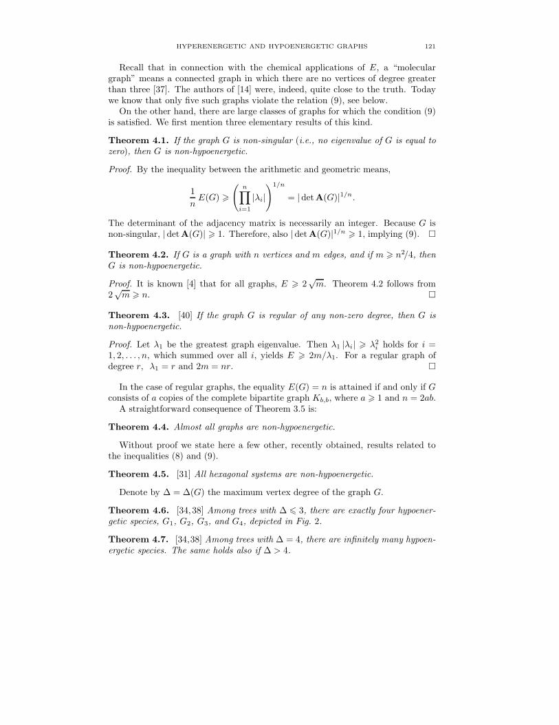
HYPERENERGETIC AND HYPOENERGETIC GRAPHS 121
Recall that in connection with the chemical applications of E, a “moleculargraph” means a connected graph in which there are no vertices of degree greaterthan three [37]. The authors of [14] were, indeed, quite close to the truth. Todaywe know that only five such graphs violate the relation (9), see below.
On the other hand, there are large classes of graphs for which the condition (9)is satisfied. We first mention three elementary results of this kind.
Theorem 4.1. If the graph G is non-singular (i.e., no eigenvalue of G is equal tozero), then G is non-hypoenergetic.
Proof. By the inequality between the arithmetic and geometric means,
1
nE(G) �
(n∏
i=1
|λi|)1/n
= | detA(G)|1/n.
The determinant of the adjacency matrix is necessarily an integer. Because G isnon-singular, | detA(G)| � 1. Therefore, also | detA(G)|1/n � 1, implying (9). �
Theorem 4.2. If G is a graph with n vertices and m edges, and if m � n2/4, thenG is non-hypoenergetic.
Proof. It is known [4] that for all graphs, E � 2√m. Theorem 4.2 follows from
2√m � n. �
Theorem 4.3. [40] If the graph G is regular of any non-zero degree, then G isnon-hypoenergetic.
Proof. Let λ1 be the greatest graph eigenvalue. Then λ1 |λi| � λ2i holds for i =1, 2, . . . , n, which summed over all i, yields E � 2m/λ1. For a regular graph ofdegree r, λ1 = r and 2m = nr. �
In the case of regular graphs, the equality E(G) = n is attained if and only if Gconsists of a copies of the complete bipartite graph Kb,b, where a � 1 and n = 2ab.
A straightforward consequence of Theorem 3.5 is:
Theorem 4.4. Almost all graphs are non-hypoenergetic.
Without proof we state here a few other, recently obtained, results related tothe inequalities (8) and (9).
Theorem 4.5. [31] All hexagonal systems are non-hypoenergetic.
Denote by Δ = Δ(G) the maximum vertex degree of the graph G.
Theorem 4.6. [34, 38] Among trees with Δ � 3, there are exactly four hypoener-getic species, G1, G2, G3, and G4, depicted in Fig. 2.
Theorem 4.7. [34,38] Among trees with Δ = 4, there are infinitely many hypoen-ergetic species. The same holds also if Δ > 4.

122 IVAN GUTMAN
In connection with Theorems 4.6 and 4.7 it is of importance to determine thetrees with maximum vertex degree Δ, having minimum energy. This problem wasrecently completely solved by Heuberger andWagner [42,43]. For an earlier attemptto treat the same problem, see [15]. Although in [15] the structure of the minimal-energy trees has not be determined, it was established that (in the general case)these differ from Volkmann trees [16, 48].
Theorem 4.8. [57] Among connected quadrangle-free graphs with Δ � 3, G1, G2,G3, and G4, and only these are hypoenergetic.
Theorem 4.9. [49] Among connected graphs with Δ � 3, G1, G2, G3, G4, andG5, and only these are hypoenergetic.
Theorem 4.10. [50] Among connected graphs with Δ � 3, G6, G7, G8, and G9,and only these have energies equal to the number of vertices.
G G G
G GGG
GG1 2 3 4 5
6 7 8 9
Figure 2. Graphs mentioned in Theorems 4.6-4.10
In connection with Theorem 4.7 it must be mentioned that if the maximumvertex degree (Δ) is sufficiently large, then it is not difficult to find hypoenergeticgraphs. For instance, the n-vertex star (with Δ = n − 1) is hypoenergetic for alln�3. In view of this, the recently reported result [67] that there exist hypoenergeticconnected unicyclic graphs for all n � 7 and hypoenergetic connected bicyclicgraphs for all n � 8 is no surprise whatsoever.
Theorem 4.11. [67] There are no hypoenergetic unicyclic graphs on n verticeswith n � 6. There exist hypoenergetic unicyclic graphs on n vertices for all n � 7.
Theorem 4.12. [67] If n is even and Δ ∈ [n/2, n − 1] or n is odd and Δ ∈[(n + 1)/2, n− 1], then for all n � 9 there exist unicyclic hypoenergetic graphs oforder n with maximum vertex degree Δ.
Theorem 4.13. [67] There are no hypoenergetic bicyclic graphs on n vertices withn = 4, n = 6, and n = 7. There exist hypoenergetic bicyclic graphs on n verticesfor n = 5 and all n � 8.

HYPERENERGETIC AND HYPOENERGETIC GRAPHS 123
Theorem 4.14. [67] If n is even and Δ ∈ [n/2 + 1, n − 1] or n is odd andΔ ∈ [(n + 1)/2, n− 1], then for all n � 9 there exist bicyclic hypoenergetic graphsof order n with maximum vertex degree Δ.
Results of the same kind as Theorems 4.11-4.14 have been obtained also forc-cyclic graphs with c � 3 [45, 51, 68]. Of these we mention here only:
Theorem 4.15. [68] There exist hypoenergetic c-cyclic graphs for any c.
5. Interlude: biregular and triregular graphs
A graph is said to be regular if all its vertices have equal degrees. We nowgeneralize this simple concept to the case when the verticex degrees assume two orthree different values.
Definition 4. Let a and b be integers, 1 � a < b. A graph is said to be (a, b)-biregular if the degrees of its vertices assume exactly two different values: a and b.
Because biregular graphs play an important role in the subsequent part of thischapter, in Fig. 3 are depicted a few examples thereof.
Figure 3. Examples of biregular graphs: a (1,2)-biregular tree(the 3-vertex path), a (1,6)-biregular tree (the 7-vertex star), a(3,4)-biregular graph, and a (2,3)-biregular graph (a hexagonalsystem).
Definition 5. Let x, a, and b be integers, 1 � x < a < b. A graph is said to be(x, a, b)-triregular if its vertices assume exactly three different values: x, a, and b.
By Theorem 4.3, the problem considered in this chapter has been completelysolved for regular graphs [40]. Hexagonal systems (mentioned in Theorem 4.5)have vertex degrees equal to 2 and 3, and therefore belong to a special class ofbiregular graphs. From the proof of Theorem 4.5 [31], it can be seen that alsoother types of biregular graphs have the same property, i.e., satisfy inequality (9).Work along these lines has recently been extended [1,33,47,52,53]. In what followswe report in due detail our [1,33] and other colleague’s [65] researches on biregulargraphs with cyclomatic number c � 2. These considerations may be of particularvalue for beginners in the field. Namely, these show how by means of relativelyelementary graph-theoretic and algebraic reasoning one can obtain not quite trivialresults on graph energy. Analogous considerations for triregular graphs can befound in [32, 53] and in the survey [54]. Tricyclic biregular graphs have also beenrecently examined [52].

124 IVAN GUTMAN
6. A lower bound for energy and its applications
In this section we obtain a lower bound for graph energy, which will be needed inthe subsequent considerations. Our starting point is the Cauchy–Schwarz inequality
n∑
i=1
xi yi �
√√√√
n∑
i=1
(xi)2n∑
i=1
(yi)2
which holds for any real numbers xi, yi, i = 1, 2, . . . , n. Setting xi = |λi|1/2 andyi = |λi|3/2, we get
(n∑
i=1
(λi)2
)4
�(
n∑
i=1
|λi|n∑
i=1
|λi|3)2
By another application of the Cauchy–Schwarz inequality,
n∑
i=1
|λi|3 =
n∑
i=1
|λi| · (λi)2 �
√√√√
n∑
i=1
(λi)2n∑
i=1
(λi)4
which substituted back into the previous inequality yields
(10)
(n∑
i=1
(λi)2
)4
�(
n∑
i=1
|λi|)2 n∑
i=1
(λi)2
n∑
i=1
(λi)4.
The k-th spectral moment of a graph G with eigenvalues λ1, λ2 . . . , λn is
Mk =Mk(G) =
n∑
i=1
(λi)k.
In view of this and the definition of graph energy, Eq. (1), the inequality (10) canbe rewritten as
(11) E �M2
√M2/M4 .
The lover bound (11) was independently discovered several times: two timesfor general graphs [24, 69] and two times for bipartite graphs [12, 58]. Recently ageneralized version thereof was obtained [70].
The importance of the bound (11) lies in the fact that the structure-dependencyof the spectral moments M2 and M4 is well known. If G is a graph with n verticesandm edges, if its vertex degrees are d1, d2, . . . , dn, and if it possesses q quadrangles,then
M2(G) = 2m(12)
M4(G) = 2
n∑
i=1
(di)2 − 2m+ 8q.(13)
Combining (11), (13), and (12), we arrive at:

HYPERENERGETIC AND HYPOENERGETIC GRAPHS 125
Theorem 6.1. Let G be a graph with n vertices and m edges, possessing q quad-rangles, and let d1, d2, . . . , dn be its vertex degrees. If the condition
(14) M2(G)
√M2(G)
M4(G)≡ 2m
√2m
∑ni=1(di)
2 − 2m+ 8q� n
is obeyed, then G is non-hypoenergetic.
The application of Theorem 6.1 will be the basis for the considerations thatfollow. Therefore it should be always kept in mind that condition (14) is a sufficient,but not a necessary condition for the validity of the inequality (9).
7. On the energy of biregular graphs
In this section we use same the notation as in Definition 4. Thus the degrees ofthe vertices of a biregular graph are denoted by a and b, and a < b.
7.1. Biregular trees. Let T be an (a, b)-biregular tree. Since trees necessarilypossess vertices of degree 1 (pendent vertices), it must be a = 1 and 1 < b � n− 1,where n is the number of vertices. This tree has at least 3 vertices and m = n− 1edges. The number of pendent vertices will be denoted by k.
From now on we search for necessary and sufficient conditions under which theinequality (14) holds.
For trees, of course, q = 0.We begin with the equalities
(15) k + nb = n
and
(16) 1 · k + b · nb = 2m = 2(n− 1),
where nb is the number of vertices of T of degree b. From (15) and (16) we have
k =2 + n(b− 2)
b− 1; nb =
n− 2
b− 1.
Further,n∑
i=1
d2i = 12 · k + b2 · nb =2 + n(b− 2)
b− 1+ b2
n− 2
b − 1= n(b+ 2)− 2(b+ 1).
By Eqs. (13) and (12), for a biregular tree T we have
(17) M2 = 2(n− 1)
and
(18) M4 = 2[n(b+ 2)− 2(b+ 1)]− 2(n− 1) = 2b(n− 2) + 2(n− 1).
Substituting the expressions (17) and (18) back into (14) we get
(19)
√4(n− 1)3
b(n− 2) + (n− 1)� n.
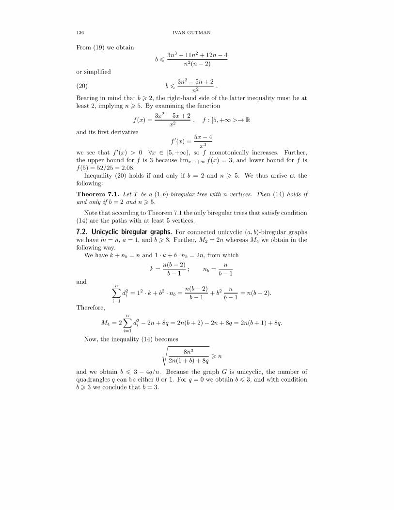
126 IVAN GUTMAN
From (19) we obtain
b � 3n3 − 11n2 + 12n− 4
n2(n− 2)
or simplified
(20) b � 3n2 − 5n+ 2
n2.
Bearing in mind that b � 2, the right-hand side of the latter inequality must be atleast 2, implying n � 5. By examining the function
f(x) =3x2 − 5x+ 2
x2, f : [5,+∞ >→ R
and its first derivative
f ′(x) =5x− 4
x3
we see that f ′(x) > 0 ∀x ∈ [5,+∞), so f monotonically increases. Further,the upper bound for f is 3 because limx→+∞ f(x) = 3, and lower bound for f isf(5) = 52/25 = 2.08.
Inequality (20) holds if and only if b = 2 and n � 5. We thus arrive at thefollowing:
Theorem 7.1. Let T be a (1, b)-biregular tree with n vertices. Then (14) holds ifand only if b = 2 and n � 5.
Note that according to Theorem 7.1 the only biregular trees that satisfy condition(14) are the paths with at least 5 vertices.
7.2. Unicyclic biregular graphs. For connected unicyclic (a, b)-biregular graphswe have m = n, a = 1, and b � 3. Further, M2 = 2n whereas M4 we obtain in thefollowing way.
We have k + nb = n and 1 · k + b · nb = 2n, from which
k =n(b − 2)
b− 1; nb =
n
b− 1
andn∑
i=1
d2i = 12 · k + b2 · nb =n(b− 2)
b− 1+ b2
n
b− 1= n(b+ 2).
Therefore,
M4 = 2
n∑
i=1
d2i − 2n+ 8q = 2n(b+ 2)− 2n+ 8q = 2n(b+ 1) + 8q.
Now, the inequality (14) becomes√
8n3
2n(1 + b) + 8q� n
and we obtain b � 3 − 4q/n. Because the graph G is unicyclic, the number ofquadrangles q can be either 0 or 1. For q = 0 we obtain b � 3, and with conditionb � 3 we conclude that b = 3.

HYPERENERGETIC AND HYPOENERGETIC GRAPHS 127
For q = 1 we obtain b � 3 − 4/n, from which we see that it must be b < 3.This, however, is impossible, implying that there is no unicyclic biregular graphwith q = 1, for which the inequality (14) holds. Thus we obtain:
Theorem 7.2. Let G be a connected unicyclic (a, b)-biregular graph with n vertices.Then (14) holds if and only if a = 1, b = 3, and q = 0.
A few examples of biregular graphs that satisfy Theorem 7.2 are shown in Fig. 4.From these examples the general structure of such graphs should be evident:
Theorem 7.3. Let G be a connected unicyclic (a, b)-biregular graph for which (14)holds. Then G is obtained from a cycle Cp, by attaching to each of its verticesexactly one pendent vertex, where p = 3 or p � 5.
Figure 4. Examples of connected quadrangle-free (1,3)-biregularunicyclic graphs.
7.3. Bicyclic biregular graphs. For bicyclic (a, b)-biregular graphs we have m =n+ 1 and the inequality (14) becomes
(21)
√4(n+ 1)3
(2a+ 2b− 1)(n+ 1)− abn+ 4q� n.
There are three possible cases (cf. Fig. 5):(a) the cycles are disjoint (they have no common vertices),(b) the cycles have a single common vertex(c) the cycles have two or more common vertices.
(a) (b) (c)
Figure 5. Types of bicyclic graphs.

128 IVAN GUTMAN
... ...
...
......
1
1
b-2
1
2 b-2
2
2 b-3
Figure 6. Sketches of (1, b)-, and (2, 3)-biregular bicyclic graphswith disjoint cycles. The vertices that connect cycles in a (1, b)-biregular graph (b � 3) are connected also with b − 3 pendentvertices, whereas all other vertices in such a graph are connectedwith b − 2 pendent vertices. In a (2, 3)-biregular graph there areonly two vertices of degree 3, those that connect cycles, while everyother vertex is of degree 2.
7.3.1. Biregular bicyclic graphs with disjoint cycles. If we have a bicyclic (a, b)-biregular graph with disjoint cycles, then there are two types of such graphs: witha = 1, b � 3, and with a = 2, b = 3, see Fig. 6.
If a = 1 and b � 3, then inequality (21) becomes√
4(n+ 1)3
b(n+ 2) + n+ 1 + 4q� n
from which
(22) b � 3n3 + (11− 4q)n2 + 12n+ 4
n3 + 2n2.
For q = 0 we obtain
b � 3n3 + 11n2 + 12n+ 4
n3 + 2n2
or simplified
(23) b � 3n2 + 5n+ 2
n2.
For b � 3, the right-hand side of the latter inequality must be at least 3. Anothercondition is n � 10, since the smallest bicyclic (1, b)-biregular graph with disjointcycles has exactly 10 vertices.
If we examine the function
f(x) =3x2 + 5x+ 2
x2, f : [10,+∞) → R
and its first derivative f ′(x) = −(5x+ 4)/x3 we conclude that f ′(x) < 0, ∀x ∈[10,+∞). Thus f is a monotonically decreasing function. The lower bound for f is3 because limx→+∞ f(x) = 3, and the upper bound for f is f(10) = 88/25 = 3.52.We conclude that it must be b = 3.

HYPERENERGETIC AND HYPOENERGETIC GRAPHS 129
For q = 1 we have
(24) b � 3n3 + 7n2 + 12n+ 4
n3 + 2n2.
Analogously, and by taking into account that n � 12, we conclude that b = 3.For q = 2 we have
(25) b � 3n3 + 3n2 + 12n+ 4
n3 + 2n2.
For n � 14 the right-hand side of the inequality (25) is less than 3 and thus thereis no bicyclic (1, b)-biregular graph with q = 2, such that the inequality (14) holds.
For bicyclic (2, 3)-biregular graphs we have√
4(n+ 1)3
3n+ 9 + 4q� n
which implies n3 + (3− 4q)n2 + 12n+ 4 � 0.For q = 0, 1, 2 we have
n3 + 3n2 + 12n+ 4 � 0
n3 − n2 + 12n+ 4 � 0
n3 − 5n2 + 12n+ 4 � 0
respectively. Each of these three inequalities holds for arbitrary n ∈ N.
Theorem 7.4. Let G be a connected bicyclic (a, b)-biregular graph with disjointcycles and let n be the number of its vertices. Then the inequality (14) holds if andonly if either a = 1, b = 3, q = 0 or a = 1, b = 3, q = 1 or a = 2, b = 3.
Some of the graphs satisfying the Theorem 7.4 are depicted in Fig. 7.
Figure 7. Connected bicyclic (1, 3)-biregular graphs with disjointcycles, with q = 0 and q = 1, and bicyclic (2, 3)-biregular graphswith disjoint cycles, with q = 0, q = 1, q = 2. In all these examplesthe number of vertices is as small as possible.

130 IVAN GUTMAN
7.3.2. Biregular bicyclic graphs whose cycles have a common vertex. If in a bicyclic(a, b)-biregular graph, the cycles share one common vertex, then we have two typesof such graphs: with a = 1, b � 4, and with a = 2, b = 4, see Fig. 8.
... ...
...
1 2 b-2
Figure 8. Connected bicyclic (1, b � 4)- and (2, 4)-biregulargraph in which cycles have one common vertex. For the (1, b)-biregular graph, b � 4, every vertex except the one belonging toboth cycles is connected with b − 2 pendent vertices. The vertexbelonging to both cycles is connected with b− 4 pendent vertices.So, every vertex belonging to the cycles has degree b. In the (2, 4)-biregular graphs there are no pendent vertices, so there is only one(common) vertex of degree 4 and every other vertex is of degree 2.
For the first type of such graphs, the inequalities (23), (24), and (25) togetherwith the condition b � 4 are not fulfilled.
For bicyclic (2, 4)-biregular graphs we have√
4(n+ 1)3
3n+ 11 + 4q� n
which is equivalent to n3 + (1− 4q)n2 + 12n+ 4 � 0. Taking q = 0, 1, 2, we obtaininequalities that are satisfied for arbitrary n ∈ N. This implies:
Theorem 7.5. Let G be a connected bicyclic (a, b)-biregular graph with n verticesin which the cycles share a single common vertex. Then condition (14) is obeyed ifand only if a = 2 and b = 4.
A few examples graphs specified in Theorem 7.5 are shown in Fig. 9.
7.3.3. Biregular bicyclic graphs whose cycles have several common vertices. If thecycles of a bicyclic (a, b)-biregular graph posses two or more common vertices, thenwe have two types of such graphs: with a = 1, b � 3, and with a = 2, b = 3, seeFig. 10.
For the graphs depicted in Fig. 10 we obtain the same results as for bicyclicgraphs with disjoint cycles, but we must add the case when q = 3 because thereexists a unique bicyclic biregular graph in which the number of quadrangles isexactly 3. This is the complete bipartite graph on 2 + 3 vertices, K2,3, shown in

HYPERENERGETIC AND HYPOENERGETIC GRAPHS 131
Figure 9. Bicyclic (2, 4)-biregular graphs in which the cycles haveone common vertex, with q = 0, 1, 2 quadrangles. In these exam-ples the number of vertices is as small as possible.
......
...
1 2 b-2
1 2 b-3
...
Figure 10. Connected bicyclic (1, b � 3)- and (2, 3)-biregulargraphs in which the cycles have two or more common vertices.Notice that the cycles of the graphs of the first type have only twocommon vertices, whereas the cycles of the graphs of the secondtype may have arbitrarily many common vertices (but more thanone, of course).
Fig. 11. From (22) for b = 3, we get the inequality −7n3 + 12n+ 4 � 0 that is notfulfilled for n = 5.
Figure 11. The only bicyclic biregular graph in which the numberof quadrangles q is 3. For this graph inequality (14) is violated.Recall that according to Theorem 4.9 this graph is hypoenergetic.
Theorem 7.6. Let G be a connected bicyclic (a, b)-biregular graph with n vertices,whose cycles have two or more common vertices. Then inequality (14) holds if andonly if a = 1, b = 3, q = 0, 1 or a = 2, b = 3, q = 0, 1, 2.
Examples of graphs for which Theorem 7.6 holds are shown in Fig. 12.

132 IVAN GUTMAN
Figure 12. Bicyclic (1, 3)-biregular graphs in which cycles havetwo common vertices and q = 0, 1, and bicyclic (2, 3)-biregulargraphs with q = 0, 1, 2.
7.3.4. Concluding remark. In this sections we established necessary and sufficientconditions for the validity of the inequality (14), for certain types of acyclic, uni-cyclic, and bicyclic graphs. In these considerations the graph energy was not men-tioned at all. Therefore, at this point it seems to be purposeful to re-state Theorem6.1:
Theorem 6.1.bis. If the graph G satisfies the inequality (14), then the energyof G is greater than (or, exceptionally, equal to) the number of vertices of G, i.e.,inequality (9) holds. Therefore G is necessarily not hypoenergetic. If, however, thegraph G does not satisfy the inequality (14), then it may be hypoenergetic, but neednot. Anyway, the search for hypoenergetic graphs must be done among those thatviolate inequality (14).
References
[1] C. Adiga, Z. Khoshbakht, I. Gutman, More graphs whose energy exceeds the number ofvertices, Iranian J. Math. Sci. Inf. 2(2) (2007), 13–19.
[2] S. Akbari, F. Moazami, S. Zare, Kneser graphs and their complements are hyperenergetic,MATCH Commun. Math. Comput. Chem. 61 (2009), 361–368.
[3] A. S. Bonifacio, N.M.M. de Abreu, C.T.M. Vinagre, I. Gutman, Grafos hiperenergeticos anao hiperenergeticos, Proceedings of XXXI Congresso Nacional de Matematica Applicada eComputacional (CNMAC 2008), Belem (Brazil), pp. 1–6.
[4] G. Caporossi, D. Cvetkovic, I. Gutman, P. Hansen, Variable neighborhood search for extremalgraphs. 2. Finding graphs with extremal energy, J. Chem. Inf. Comput. Sci. 39 (1999), 984–996.
[5] C.A. Coulson, On the calculation of the energy in unsaturated hydrocarbon molecules, Proc.Cambridge Phil. Soc. 36 (1940), 201–203.
[6] C.A. Coulson, B. O’Leary, R.B. Mallion, Huckel Theory for Organic Chemists, AcademicPress, London, 1978.
[7] D. Cvetkovic, M. Doob, H. Sachs, Spectra of Graphs – Theory and Application, third ed.,Barth Verlag, Heidelberg, 1995.

HYPERENERGETIC AND HYPOENERGETIC GRAPHS 133
[8] D.M. Cvetkovic, I. Gutman, The algebraic multiplicity of the number zero in the spectrumof a bipartite graph Mat. Vesnik (Beograd) 9 (1972), 141–150.
[9] D. Cvetkovic, I. Gutman, The computer system GRAPH: A useful tool in chemical graphtheory, J. Comput. Chem. 7 (1986), 640–644.
[10] D. Cvetkovic, I. Gutman, V. Kovacevic-Vujcic, Eds. Grafovi, optimjizacija, hemija - Zapisio radu jednog naucnog projekta [Graphs, Optimization, Chemistry - Notes on the Work ofa Scientific Project], Akademska misao, Beograd, 2007.
[11] D. Cvetkovic, P. Rowlinson, S. Simic, An Introduction to the Theory of Graph Spectra,Cambridge Univ. Press, Cambridge, 2010.
[12] J. A. de la Pena, L. Mendoza, J. Rada, Comparing momenta and π-electron energy of ben-zenoid molecules, Discr. Math. 302 (2005), 77–84.
[13] J. R. Dias, Molecular Orbital Calculations Using Chemical Graph Theory, Springer-Verlag,Berlin, 1993.
[14] W. England, K. Ruedenberg, Why is the delocalization energy negative and why is it propor-tional to the number of π electrons?, J. Am. Chem. Soc. 95 (1973), 8769–8775.
[15] M. Fischermann, I. Gutman, A. Hoffmann, D. Rautenbach, D. Vidovic, L. Volkmann, Ex-tremal chemical trees, Z. Naturforsch. 57a (2002), 49–52.
[16] M. Fischermann, A. Hoffmann, D. Rautenbach, L. Szekely, L. Volkmann, Wiener index versusmaximum degree in trees, Discr. Appl. Math. 122 (2002), 127–137.
[17] A. Graovac, I. Gutman, N. Trinajstic, Topological Approach to the Chemistry of ConjugatedMolecules, Springer-Verlag, Berlin, 1977.
[18] A. Graovac, I. Gutman, N. Trinajstic, T. Zivkovic, Graph theory and molecular orbitals.Application of Sachs theorem, Theor. Chim. Acta 26 (1972), 67–78.
[19] H.H. Gunthard, H. Primas, Zusammenhang von Graphentheorie und MO-Theorie vonMolekeln mit Systemen konjugierter Bindungen, Helv. Chim. Acta 39 (1956), 1645–1653.
[20] I. Gutman, Acyclic systems with extremal Huckel π-electron energy, Theor. Chim. Acta 45(1977), 79–87.
[21] I. Gutman, The energy of a graph, Ber. Math-Statist. Sekt. Forschungsz. Graz 103 (1978),1–22.
[22] I. Gutman, Acyclic conjugated molecules, trees and their energies, J. Math. Chem. 1 (1987),123–143.
[23] I. Gutman, Total π-electron energy of benzenoid hydrocarbons, Topics Curr. Chem. 162(1992), 29–63.
[24] I. Gutman, On the energy of quadrangle-free graphs, Coll. Sci. Papers Fac. Sci. Kragujevac18 (1996), 75–82.
[25] I. Gutman, Hyperenergetic molecular graphs, J. Serb. Chem. Soc. 64 (1999), 199–205.
[26] I. Gutman, The energy of a graph: Old and new results, in: A. Betten, A. Kohnert, R. Laue,A. Wassermann, Eds. Algebraic Combinatorics and Applications, Springer-Verlag, Berlin,2001, pp. 196–211.
[27] I. Gutman, Impact of the Sachs theorem on theoretical chemistry: A participant’s testimony,MATCH Commun. Math. Comput. Chem. 48 (2003), 17–34.
[28] I. Gutman, Topology and stability of conjugated hydrocarbons. The dependence of totalπ-electron energy on molecular topology, J. Serb. Chem. Soc. 70 (2005), 441–456.
[29] I. Gutman, Chemical graph theory – The mathematical connection, in: J. R. Sabin, E. J.Brandas, Eds. Advances in Quantum Chemistry 51, Elsevier, Amsterdam, 2006, pp. 125–138.
[30] I. Gutman Dragos Cvetkovic i teorijska hemija [Dragos Cvetkovic and theoretical chemistry],in: D. Cvetkovic, Grafovi kao inspiracija, Akademska misao, Beograd, 2006, pp. 26–31.
[31] I. Gutman, On graphs whose energy exceeds the number of vertices, Lin. Algebra Appl. 429(2008), 2670–2677.
[32] I. Gutman, Y. Hou, H.B. Walikar, H. S. Ramane, P.R. Hampiholi, No Huckel graph ishyperenergetic, J. Serb. Chem. Soc. 65 (2000), 799–801.

134 IVAN GUTMAN
[33] I. Gutman, A. Klobucar, S. Majstorovic, C. Adiga, Biregular graphs whose energy exceedsthe number of vertices, MATCH Commun. Math. Comput. Chem. 62 (2009), 499–508.
[34] I. Gutman, X. Li, Y. Shi, J. Zhang, Hypoenergetic trees, MATCH Commun. Math. Comput.Chem. 60 (2008), 415–426.
[35] I. Gutman, X. Li, J. Zhang, Graph energy, in: M. Dehmer, F. Emmert-Streib, Eds. Analysisof Complex Networks. From Biology to Linguistics, Wiley–VCH, Weinheim, 2009, pp. 145–174.
[36] I. Gutman, L. Pavlovic, The energy of some graphs with large number of edges, Bull. Acad.Serbe Sci. Arts (Cl. Sci. Math. Natur.) 118 (1999), 35–50.
[37] I. Gutman, O.E. Polansky, Mathematical Concepts in Organic Chemistry, Springer-Verlag,Berlin, 1986.
[38] I. Gutman, S. Radenkovic, Hypoenergetic molecular graphs, Indian J. Chem. 46A (2007),1733–1736.
[39] I. Gutman, T. Soldatovic, (n,m)-Type approximations for total π-electron energy of ben-zenoid hydrocarbons, MATCH Commun. Math. Comput. Chem. 44 (2001), 169–182.
[40] I. Gutman, S. Zare Firoozabadi, J. A. de la Pena, J. Rada, On the energy of regular graphs,MATCH Commun. Math. Comput. Chem. 57 (2007), 435–442.
[41] G.G. Hall, The bond orders of alternant hydrocarbon molecules, Proc. Roy. Soc. A 229(1955), 251–259.
[42] C. Heuberger, S. G. Wagner, Chemical trees minimizing energy and Hosoya index, J. Math.Chem. 46 (2009), 214–230.
[43] C. Heuberger, S. G. Wagner, On a class of extremal trees for various indices, MATCHCommun. Math. Comput. Chem. 62 (2009), 437–464.
[44] Y. Hou, I. Gutman, Hyperenergetic line graphs, MATCH Commun. Math. Comput. Chem.43 (2001), 29–39.
[45] X. Hui, H. Deng, Solutions of some unsolved problems on hypoenergetic unicyclic, bicyclicand tricyclic graphs, MATCH Commun. Math. Comput. Chem. 64 (2010), 231–238.
[46] J. H. Koolen, V. Moulton, I. Gutman, D. Vidovic, More hyperenergetic molecular graphs, J.Serb. Chem. Soc. 65 (2000), 571–575.
[47] S. Li, X. Li, H. Ma, I. Gutman, On triregular graphs whose energy exceeds the number ofvertices, MATCH Commun. Math. Comput. Chem. 64 (2010), 201–216.
[48] W. Li, X. Li, I. Gutman, Volkmann trees and their molecular structure descriptors, in: I.Gutman, B. Furtula, Eds. Novel Molecular Structure Descriptors – Theory and ApplicationsII , Univ. Kragujevac, Kragujevac, 2010, pp. 231–246.
[49] X. Li, H. Ma, All hypoenergetic graphs with maximum degree at most 3, Lin. Algebra Appl.431 (2009), 2127–2133.
[50] X. Li, H. Ma All connected graphs with maximum degree at most 3 whose energies are equalto the number of vertices, MATCH Commun. Math. Comput. Chem. 64 (2010), 7–24.
[51] X. Li, H. Ma, Hypoenergetic and strongly hypoenergetic k-cyclic graphs, MATCH Commun.Math. Comput. Chem. 64 (2010), 41–60.
[52] S. Majstorovic, I. Gutman, A. Klobucar, Tricyclic biregular graphs whose energy exceeds thenumber of vertices, Math. Commun. 15 (2010), 213–222.
[53] S. Majstorovic, A. Klobucar, I. Gutman, Triregular graphs whose energy exceeds the numberof vertices, MATCH Commun. Math. Comput. Chem. 62 (2009), 509–524.
[54] S. Majstorovic, A. Klobucar, I. Gutman, Selected topics from the theory of graph energy:hypoenergetic graphs, in: D. Cvetkovic, I. Gutman, Eds. Applications of Graph Spectra,Math. Inst., Belgrade, 2009, pp. 65–105.
[55] B. J. McClelland, Properties of the latent roots of a matrix: The estimation of π-electronenergies, J. Chem. Phys. 54 (1971), 640–643.
[56] V. Nikiforov, The energy of graphs and matrices, J. Math. Anal. Appl. 326 (2007), 1472–1475.
[57] V. Nikiforov, The energy of C4-free graphs of bounded degree, Lin. Algebra Appl. 428 (2008),2569–2573.

HYPERENERGETIC AND HYPOENERGETIC GRAPHS 135
[58] J. Rada, A. Tineo, Upper and lower bounds for energy of bipartite graphs, J. Math. Anal.Appl. 289 (2004), 446–455.
[59] K. Ruedenberg, Quantum mechanics of mobile electrons in conjugated bond systems. III.Topological matrix as generatrix of bond orders, J. Chem. Phys. 34 (1961), 1884–1891.
[60] X. Shen, Y. Hou, I. Gutman, X. Hui, Hyperenergetic graphs and cyclomatic number, Bull.Acad. Serbe Sci. Arts (Cl. Sci. Math. Natur.) 141 (2010), 1–8.
[61] D. Stevanovic, I. Stankovic, Remarks on hyperenergetic circulant graphs, Lin. Algebra Appl.400 (2005), 345–348.
[62] A. Streitwieser, Molecular Orbital Theory for Organic Chemists, Wiley, New York, 1961.[63] H.B. Walikar, I. Gutman, P. R. Hampiholi, H. S. Ramane, Non–hyperenergetic graphs Graph
Theory Notes New York 41 (2001), 14–16.[64] H.B. Walikar, H. S. Ramane, P.R. Hampiholi, On the energy of a graph in: R. Balakrishnan,
H. M. Mulder, A. Vijayakumar, Eds. Graph Connections, Allied Publishers, New Delhi, 1999,pp. 120–123.
[65] L. Xu, On biregular graphs whose energy exceeds the number of vertices, MATCH Commun.Math. Comput. Chem. 66 (2011), in press.
[66] K. Yates, Huckel Molecular Orbital Theory, Academic Press, New York, 1978.[67] Z. You, B. Liu, On hypoenergetic unicyclic and bicyclic graphs, MATCH Commun. Math.
Comput. Chem. 61 (2009), 479–486.[68] Z. You, B. Liu, I. Gutman, Note on hypoenergetic graphs, MATCH Commun. Math. Comput.
Chem. 62 (2009), 491–498.[69] B. Zhou, On the energy of a graph, Kragujevac J. Sci. 26 (2004), 5–12.[70] B. Zhou, I. Gutman, J.A. de la Pena, J. Rada, L. Mendoza, On spectral moments and energy
of graphs, MATCH Commun. Math. Comput. Chem. 57 (2007), 183–191.


Ivan Gutman and Bojana Borovicanin
NULLITY OF GRAPHS: AN UPDATED SURVEY
Abstract. The nullity η = η(G) of a graph G is the multiplicity ofthe number zero in the spectrum of G . The chemical importance ofthis graph-spectrum based invariant lies in the fact, that within theHuckel molecular orbital model, if η(G) > 0 for the molecular graphG , then the corresponding chemical compound is highly reactive andunstable, or nonexistent. This chapter in an updated version of thean earlier survey [B. Borovicanin, I. Gutman, Nullity of graphs, in:D. Cvetkovic, I. Gutman, Eds. Applications of Graph Spectra, Math.Inst., Belgrade, 2009, pp. 107–122] and outlines both the chemicallyrelevant aspects of η (most of which were obtained in the 1970s and1980s) and the general mathematical results on η obtained recently.
Mathematics Subject Classification (2010): 05C50; 05C90; 92E10
Keywords : nullity (of graph); zero eigenvalue (of graph); spectrum(of graph); chemistry

Contents
1. Graph nullity and its chemical applications 1382. Elementary properties of nullity 1403. Relations between nullity and graph structure 1424. Graphs with maximum nullity 145References 152
1. Graph nullity and its chemical applications
This chapter is an updated, extended, and modified version of the survey [3] thatwas a part of the booklet “Applications of Graph Spectra”. Since the completionof [3], a number of relevant results came to the authors’ attention, that now areappropriately taken care of.
Let G be a graph of order n, having vertex set V (G) and edge set E(G). LetA(G) be the adjacency matrix of G. The graph G is said to be singular (resp. non-singular) if its adjacency matrix A(G) is singular (resp. non-singular). The nullityof G, denoted by η = η(G), is the algebraic multiplicity of the number zero in thespectrum of G.1
In addition to its evident relevance in “pure” spectral graph theory, the nul-lity has a noteworthy application in chemistry. The recognition of this fact, firstoutlined in [8], was not only an important discovery per se, but happened to bethe starting point of an unprecedented activity in theoretical and mathematicalchemistry, resulting in thousands of published papers, and leading to a new field ofresearch, nowadays referred to as Chemical Graph Theory [13, 19, 23, 40].
In order to explain the role of the nullity of graphs in chemistry, we need to recalla few basic facts from the quantum theory of molecules [12]. The behavior of theelectrons in molecules is considered to be responsible for the majority of propertiesof chemical compounds. This behavior is governed by laws of quantum theory andis described by the so-called Schrodinger equation. Finding the solutions of theSchrodinger equation is one of the main tasks of quantum chemistry.
In an early stage of quantum chemistry, during the time when computers werenot available, the German theoretical chemist Erich Huckel proposed an approxi-mate method for solving the Schrodinger equation for a special (for chemistry veryimportant) class of organic molecules, the so-called unsaturated conjugated hydro-carbons [28]. Nowadays, this method is known under the name Huckel molecularorbital (HMO) theory [5, 12, 41].
A quarter of century was needed to recognize that the mathematics on whichthe HMO theory is based is graph spectral theory [20, 35]. In a nutshell: The(approximate) energies E1, E2, . . . that the electrons may possess are related to the
1The symbol η for nullity was first used by I. G. in his correspondence with Dragos Cvetkovic,which eventually resulted in the paper [8]. The choice for η was fully arbitrary. Yet, nowadaysthis symbol is used by the majority of scholars. Another notation for nullity is n0.

NULLITY OF GRAPHS: AN UPDATED SURVEY 139
eigenvalues λ1, λ2, . . . of a so-called “molecular graph” as
Ej = α+ β λj , j = 1, 2, . . . , n
where α and β are certain constants; for more detail see [19, 23]. Because β < 0, ifthe graph eigenvalues are labelled in the usual non-increasing manner as
λ1 � λ2 � · · · � λn
then E1 is the lowest energy level, E2 is the second–lowest energy level, etc.Each energy level in a molecule can be occupied by at most two electrons. Usu-
ally, the total number of electrons to which HMO theory is applied is equal to n,and n is most frequently an even number. Usually, En/2+1 < En/2 or, what is thesame, λn/2 > λn/2+1.
If so, then in order to achieve the lowest-energy state of the underlying molecule,it has to possess two (= the maximum possible number) of electrons with energyE1, two (= the maximum possible number) of electrons with energy E2, . . . and two(= the maximum possible number) of electrons with energy En/2. This will resultin a stable arrangement of electrons; in the language of theoretical chemistry, themolecule will have a “closed–shell electron configuration”.
If, however, En/2+1 = En/2, then a total of four electrons could fill the two“degenerate” energy levels. Because the number of available electrons is only two,an irregular and unstable arrangement of electrons will result; in the language oftheoretical chemistry, the molecule will have an “open–shell electron configuration”.
The above described filling of the energy levels with electrons is in quantumchemistry referred to as the Aufbau principle (a word originating from Germanlanguage). Details on this matter can be found elsewhere [33].
Molecules with an open-shell electron configuration are known to be highly re-active and in many cases are simply not capable of existence.
We now show how the nullity of the molecular graph is related to the closed/open-shell character of the underlying molecule.
Long before the above-sketched graph-spectral connections were envisaged, someimportant results in HMO theory were discovered. One of these is the so-called“Pairing theorem” [6]. According to it, for the majority of unsaturated conjugatedhydrocarbons, the eigenvalues of the molecular graph are “paired”, so that
(1) λj = −λn−j+1
holds for all j = 1, 2, . . . , n. In the language of HMO theory, the hydrocarbonsto which the Pairing theorem applies are referred to as “alternant”. With today’sknowledge it is straightforward to recognize that an unsaturated conjugated hydro-carbon is “alternant” if and only if its molecular graph is bipartite. Indeed, therelation (1) is a well known spectral property of bipartite graphs [7].
An immediate consequence of the Pairing theorem is that a molecular graph witheven number of vertices has either nullity zero (in which case λn/2 > 0 > λn/2+1),or its nullity is an even positive integer (in which case λn/2 = λn/2+1 = 0). InHMO theory this means the following [32]:
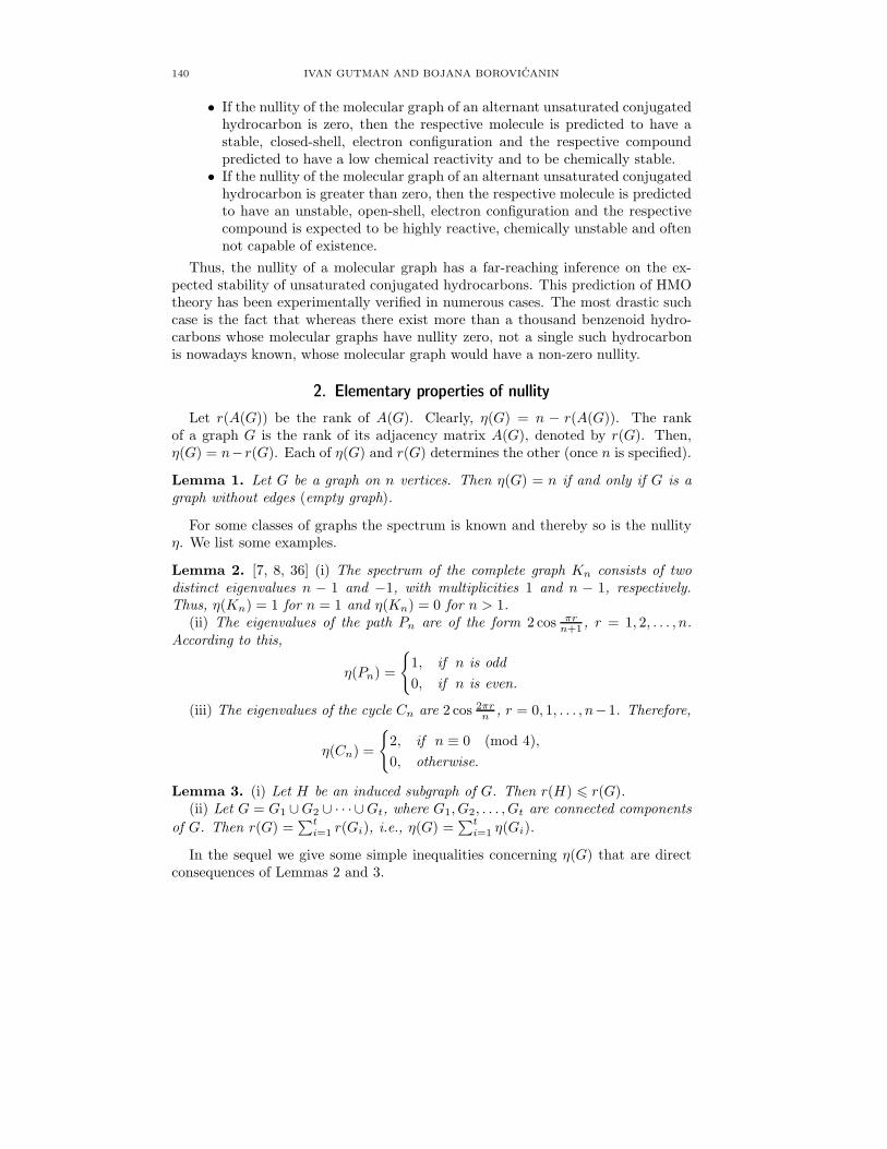
140 IVAN GUTMAN AND BOJANA BOROVICANIN
• If the nullity of the molecular graph of an alternant unsaturated conjugatedhydrocarbon is zero, then the respective molecule is predicted to have astable, closed-shell, electron configuration and the respective compoundpredicted to have a low chemical reactivity and to be chemically stable.
• If the nullity of the molecular graph of an alternant unsaturated conjugatedhydrocarbon is greater than zero, then the respective molecule is predictedto have an unstable, open-shell, electron configuration and the respectivecompound is expected to be highly reactive, chemically unstable and oftennot capable of existence.
Thus, the nullity of a molecular graph has a far-reaching inference on the ex-pected stability of unsaturated conjugated hydrocarbons. This prediction of HMOtheory has been experimentally verified in numerous cases. The most drastic suchcase is the fact that whereas there exist more than a thousand benzenoid hydro-carbons whose molecular graphs have nullity zero, not a single such hydrocarbonis nowadays known, whose molecular graph would have a non-zero nullity.
2. Elementary properties of nullity
Let r(A(G)) be the rank of A(G). Clearly, η(G) = n − r(A(G)). The rankof a graph G is the rank of its adjacency matrix A(G), denoted by r(G). Then,η(G) = n−r(G). Each of η(G) and r(G) determines the other (once n is specified).
Lemma 1. Let G be a graph on n vertices. Then η(G) = n if and only if G is agraph without edges (empty graph).
For some classes of graphs the spectrum is known and thereby so is the nullityη. We list some examples.
Lemma 2. [7, 8, 36] (i) The spectrum of the complete graph Kn consists of twodistinct eigenvalues n − 1 and −1, with multiplicities 1 and n − 1, respectively.Thus, η(Kn) = 1 for n = 1 and η(Kn) = 0 for n > 1.
(ii) The eigenvalues of the path Pn are of the form 2 cos πrn+1 , r = 1, 2, . . . , n.
According to this,
η(Pn) =
{1, if n is odd
0, if n is even.
(iii) The eigenvalues of the cycle Cn are 2 cos 2πrn , r = 0, 1, . . . , n−1. Therefore,
η(Cn) =
{2, if n ≡ 0 (mod 4),
0, otherwise.
Lemma 3. (i) Let H be an induced subgraph of G. Then r(H) � r(G).(ii) Let G = G1 ∪G2 ∪ · · · ∪Gt, where G1, G2, . . . , Gt are connected components
of G. Then r(G) =∑t
i=1 r(Gi), i.e., η(G) =∑t
i=1 η(Gi).
In the sequel we give some simple inequalities concerning η(G) that are directconsequences of Lemmas 2 and 3.

NULLITY OF GRAPHS: AN UPDATED SURVEY 141
Recall that the path P is a graph with V (P ) = {v1, v2, . . . , vk} and E(P ) ={v1v2, v2v3, . . . , vk−1vk}, where the vertices v1, v2, . . . , vk are all distinct. We saythat P is a path from v1 to vk, or a (v1, vk)-path. It can be denoted by Pk, wherek is its length. The distance d(x, y) in G of two vertices x, y is the length of ashortest (x, y)-path in G; if no such path exists, we define d(x, y) to be infinite.The greatest distance between any two vertices in G is the diameter of G, denotedby diam(G).
Lemma 4. [11] Let G be a simple graph on n vertices, and let the complete graphKp be a subgraph of G, where 2 � p � n. Then η(G) � n− p.
A clique of a simple graphG is a complete subgraph of G. A clique S is maximumif G has no clique S′ with |V (S′)| > |V (S)|. The number of vertices in a maximumclique of G is called the clique number of G and is denoted by ω(G).
The following inequality is clear from the previous result.
Corollary 1. [11] Let G be a simple non-empty graph on n vertices. Then η(G) +ω(G) � n.
From Lemma 3 and Lemma 2(iii) we arrive at:
Lemma 5. [11] Let G be a simple graph on n vertices and let the cycle Cp be aninduced subgraph of G, where 3 � p � n. Then
η(G) �{n− p+ 2, if p ≡ 0 (mod 4),
n− p, otherwise.
The length of the shortest cycle in a graph G is the girth of G, denoted by gir(G).A relation between η(G) and gir(G) is given by:
Corollary 2. [11] If G is a simple graph on n vertices, and G has at least onecycle, then
η(G) �{n− gir(G) + 2, if gir(G) ≡ 0 (mod 4),
n− gir(G), otherwise.
If we bear in mind Lemma 2(ii) and Lemma 3, the following result is obvious.
Lemma 6. [11] Let G be a simple graph on n vertices and let the path Pk be aninduced subgraph of G, where 2 � k � n. Then
η(G) �{n− k + 1, if k is odd,
n− k, otherwise.
Corollary 3. [11] Suppose that x and y are two vertices in G and that there existsan (x, y)-path in G. Then
η(G) �{n− d(x, y), if d(x, y) is even,
n− d(x, y)− 1, otherwise.

142 IVAN GUTMAN AND BOJANA BOROVICANIN
Corollary 4. [11] Suppose G is a simple connected graph on n vertices. Then
η(G) �{n− diam(G), if diam(G) is even,
n− diam(G)− 1, otherwise.
3. Relations between nullity and graph structure
In the general case, the problem of finding connections between the structure ofa graph G and its nullity seems to be difficult. For example, η(G) is not determinedby the set of vertex degrees of G (see Fig. 1)
Figure 1
In what follows we consider mostly bipartite graphs, although some of the the-orems stated below can be extended to non-bipartite graphs (see [9]).
Before proceeding we need some definitions. A matching of G is a collectionof independent (mutually non-adjacent) edges of G. A maximum matching is amatching with the maximum possible number of edges. The size of a maximummatching of G, i.e., the maximum number of independent edges of G, is denotedby m = m(G).
Denote by PG(λ) the characteristic polynomial of G. Let
PG(λ) = |λI −A| = λn + a1λn−1 + · · ·+ an
Then [7]
(2) ai =∑
U
(−1)p(U) 2c(U) (i = 1, 2, . . . , n),
where the sum is over all subgraphs U of G consisting of disjoint edges and cyclesand having exactly i vertices (called “basic figures”). If U is such a subgraph, thenp(U) is the number of its components, of which c(U) components are cycles.
For some special classes of bipartite graphs it is possible to find relatively easilythe relation between the structure of G and η(G). The problem is solved for treesby the following theorem [8].
Theorem 1. [8] Let T be a tree on n � 1 vertices and let m be the size of itsmaximum matching. Then its nullity is equal to η(T ) = n− 2m.
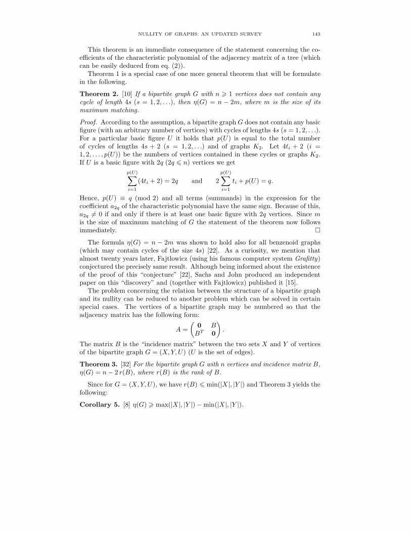
NULLITY OF GRAPHS: AN UPDATED SURVEY 143
This theorem is an immediate consequence of the statement concerning the co-efficients of the characteristic polynomial of the adjacency matrix of a tree (whichcan be easily deduced from eq. (2)).
Theorem 1 is a special case of one more general theorem that will be formulatein the following.
Theorem 2. [10] If a bipartite graph G with n � 1 vertices does not contain anycycle of length 4s (s = 1, 2, . . .), then η(G) = n − 2m, where m is the size of itsmaximum matching.
Proof. According to the assumption, a bipartite graph G does not contain any basicfigure (with an arbitrary number of vertices) with cycles of lengths 4s (s = 1, 2, . . .).For a particular basic figure U it holds that p(U) is equal to the total numberof cycles of lengths 4s + 2 (s = 1, 2, . . .) and of graphs K2. Let 4ti + 2 (i =1, 2, . . . , p(U)) be the numbers of vertices contained in these cycles or graphs K2.If U is a basic figure with 2q (2q � n) vertices we get
p(U)∑
i=1
(4ti + 2) = 2q and 2
p(U)∑
i=1
ti + p(U) = q.
Hence, p(U) ≡ q (mod 2) and all terms (summands) in the expression for thecoefficient a2q of the characteristic polynomial have the same sign. Because of this,a2q �= 0 if and only if there is at least one basic figure with 2q vertices. Since mis the size of maximum matching of G the statement of the theorem now followsimmediately. �
The formula η(G) = n − 2m was shown to hold also for all benzenoid graphs(which may contain cycles of the size 4s) [22]. As a curiosity, we mention thatalmost twenty years later, Fajtlowicz (using his famous computer system Grafitty)conjectured the precisely same result. Although being informed about the existenceof the proof of this “conjecture” [22], Sachs and John produced an independentpaper on this “discovery” and (together with Fajtlowicz) published it [15].
The problem concerning the relation between the structure of a bipartite graphand its nullity can be reduced to another problem which can be solved in certainspecial cases. The vertices of a bipartite graph may be numbered so that theadjacency matrix has the following form:
A =
(0 BBT 0
).
The matrix B is the “incidence matrix” between the two sets X and Y of verticesof the bipartite graph G = (X,Y, U) (U is the set of edges).
Theorem 3. [32] For the bipartite graph G with n vertices and incidence matrix B,η(G) = n− 2 r(B), where r(B) is the rank of B.
Since for G = (X,Y, U), we have r(B) � min(|X |, |Y |) and Theorem 3 yields thefollowing:
Corollary 5. [8] η(G) � max(|X |, |Y |)−min(|X |, |Y |).
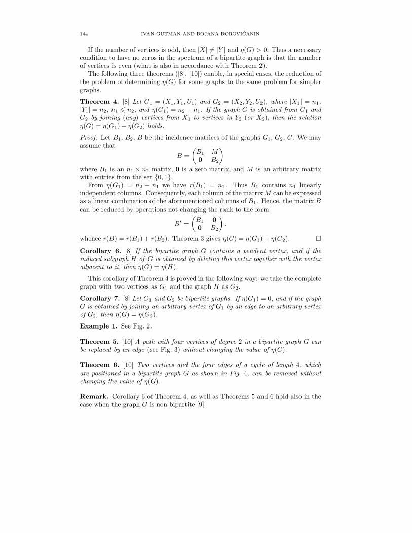
144 IVAN GUTMAN AND BOJANA BOROVICANIN
If the number of vertices is odd, then |X | �= |Y | and η(G) > 0. Thus a necessarycondition to have no zeros in the spectrum of a bipartite graph is that the numberof vertices is even (what is also in accordance with Theorem 2).
The following three theorems ([8], [10]) enable, in special cases, the reduction ofthe problem of determining η(G) for some graphs to the same problem for simplergraphs.
Theorem 4. [8] Let G1 = (X1, Y1, U1) and G2 = (X2, Y2, U2), where |X1| = n1,|Y1| = n2, n1 � n2, and η(G1) = n2 − n1. If the graph G is obtained from G1 andG2 by joining (any) vertices from X1 to vertices in Y2 (or X2), then the relationη(G) = η(G1) + η(G2) holds.
Proof. Let B1, B2, B be the incidence matrices of the graphs G1, G2, G. We mayassume that
B =
(B1 M0 B2
)
where B1 is an n1 × n2 matrix, 0 is a zero matrix, and M is an arbitrary matrixwith entries from the set {0, 1}.
From η(G1) = n2 − n1 we have r(B1) = n1. Thus B1 contains n1 linearlyindependent columns. Consequently, each column of the matrixM can be expressedas a linear combination of the aforementioned columns of B1. Hence, the matrix Bcan be reduced by operations not changing the rank to the form
B′ =(B1 00 B2
).
whence r(B) = r(B1) + r(B2). Theorem 3 gives η(G) = η(G1) + η(G2). �Corollary 6. [8] If the bipartite graph G contains a pendent vertex, and if theinduced subgraph H of G is obtained by deleting this vertex together with the vertexadjacent to it, then η(G) = η(H).
This corollary of Theorem 4 is proved in the following way: we take the completegraph with two vertices as G1 and the graph H as G2.
Corollary 7. [8] Let G1 and G2 be bipartite graphs. If η(G1) = 0, and if the graphG is obtained by joining an arbitrary vertex of G1 by an edge to an arbitrary vertexof G2, then η(G) = η(G2).
Example 1. See Fig. 2.
Theorem 5. [10] A path with four vertices of degree 2 in a bipartite graph G canbe replaced by an edge (see Fig. 3) without changing the value of η(G).
Theorem 6. [10] Two vertices and the four edges of a cycle of length 4, whichare positioned in a bipartite graph G as shown in Fig. 4, can be removed withoutchanging the value of η(G).
Remark. Corollary 6 of Theorem 4, as well as Theorems 5 and 6 hold also in thecase when the graph G is non-bipartite [9].

NULLITY OF GRAPHS: AN UPDATED SURVEY 145
Figure 2
Figure 3
Figure 4
Example 2. See Fig. 5.
4. Graphs with maximum nullity
If we bear in mind Lemmas 1 and 4, it is obvious that 0 � η(G) � n− 2 if G isa simple non-empty graph on n vertices.

146 IVAN GUTMAN AND BOJANA BOROVICANIN
Figure 5
A natural problem is to characterize the extremal graphs whose nullities attainthe upper bound n− 2 and the second upper bound n− 3.
Theorem 7. [11] Suppose that G is a simple graph on n vertices and G has noisolated vertices. Then
(i) η(G) = n − 2 if and only if G is isomorphic to a complete bipartite graphKn1,n2 , where n1 + n2 = n, n1, n2 > 0.
(ii) η(G) = n − 3 if and only if G is isomorphic to a complete tripartite graphKn1,n2,n3 , where n1 + n2 + n3 = n, n1, n2, n3 > 0.
Several results on the graphs satisfying η = n − t for some fixed value t, t > 3were obtained. Before stating them we give some necessary definitions.
Let Gn be the set of all n-vertex graphs, and let [0, n] = {0, 1, . . . , n}. A subsetN of [0, n] is said to be the nullity set of Gn provided that for any k ∈ N , thereexists at least one graph G ∈ Gn such that η(G) = k.
A connected simple graph on n vertices is said to be unicyclic if it has n edgesand bicyclic if it has n + 1 edges. Denote by Un and Bn the set of all n-vertexunicyclic and bicyclic graphs, respectively. For convenience, let Tn denote the setof n-vertex trees.
First we determine all graphs with pendent vertices that attain the third-maxim-um nullity n− 4 and the fourth-maximum nullity n− 5, using the results of Li [30].Then we proceed recursively, as in [30], to construct all graphs having pendentvertices with η(G) > 0.
Let G∗1 be an n-vertex graph obtained from a complete bipartite graph Kr,s and
a star K1,t by identifying a vertex of Kr,s with the center of K1,t, where r, s, t � 1and r + s + t = n. Let K1,l,m be a complete tripartite graph with the maximum-degree vertex v, where l,m > 0. Then let G2 be the n-vertex graph created fromK1,l,m and a star K1,p by identifying the vertex v with the center of K1,p, wherel,m, p � 1 and l +m+ p+ 1 = n.
Theorem 8. [30] Let G be a connected n-vertex graph with pendent vertices. Thenη(G) = n − 4 if and only if G is isomorphic to the graph G∗
1 or G∗2, where G
∗1 is
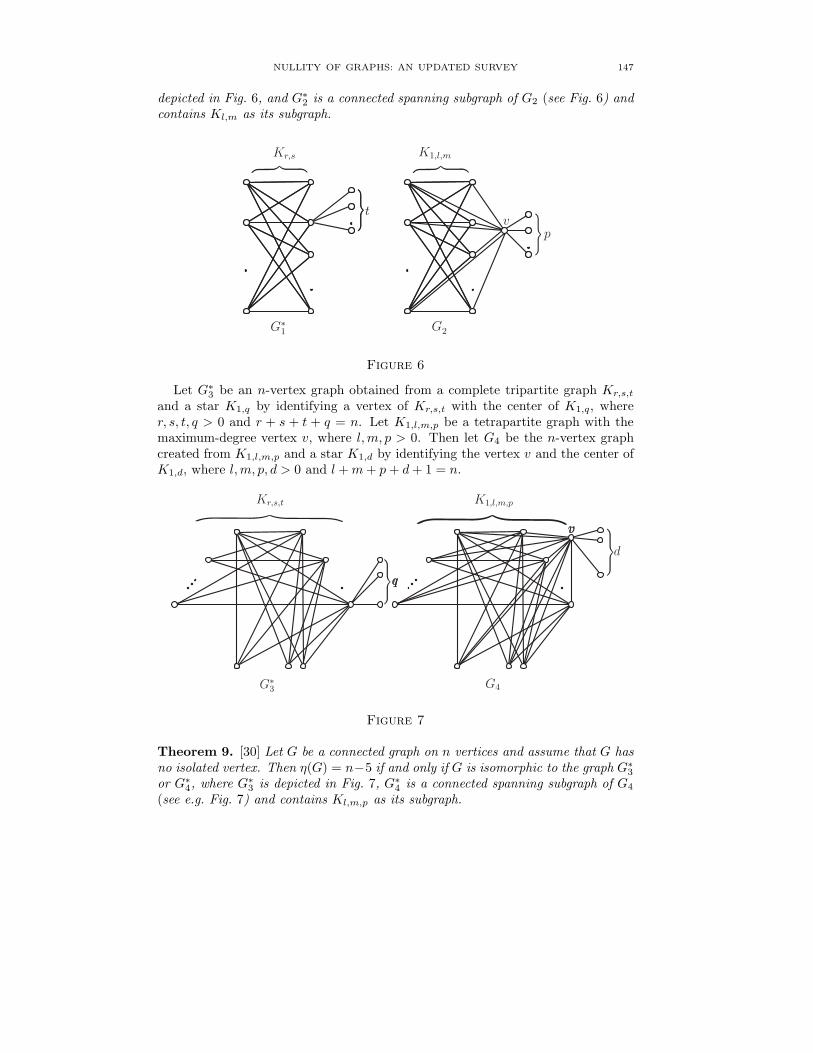
NULLITY OF GRAPHS: AN UPDATED SURVEY 147
depicted in Fig. 6, and G∗2 is a connected spanning subgraph of G2 (see Fig. 6) and
contains Kl,m as its subgraph.
Figure 6
Let G∗3 be an n-vertex graph obtained from a complete tripartite graph Kr,s,t
and a star K1,q by identifying a vertex of Kr,s,t with the center of K1,q, wherer, s, t, q > 0 and r + s + t + q = n. Let K1,l,m,p be a tetrapartite graph with themaximum-degree vertex v, where l,m, p > 0. Then let G4 be the n-vertex graphcreated from K1,l,m,p and a star K1,d by identifying the vertex v and the center ofK1,d, where l,m, p, d > 0 and l +m+ p+ d+ 1 = n.
Figure 7
Theorem 9. [30] Let G be a connected graph on n vertices and assume that G hasno isolated vertex. Then η(G) = n−5 if and only if G is isomorphic to the graph G∗
3
or G∗4, where G
∗3 is depicted in Fig. 7, G∗
4 is a connected spanning subgraph of G4
(see e.g. Fig. 7) and contains Kl,m,p as its subgraph.

148 IVAN GUTMAN AND BOJANA BOROVICANIN
Using similar reasoning as in Theorems 8 and 9, we may proceed recursively toconstruct all n-vertex graphs having pendent vertices with η(G) = n − 6, n − 7,n− 8, and so on. In that way, all n-vertex graphs with pendent vertices satisfyingη(G) > 0 can be determined [30]. Recently, also graphs with pendent trees wereexamined with regard to their nullity [18].
In the sequel we formulate some results on the extremal nullity of trees, unicyclicand bicyclic graphs. We also give the characterization of their nullity sets.
For an n-vertex tree, if it is a complete bipartite graph, then the tree shouldbe the star. Since any complete tripartite graph is cyclic, there does not exist atree that is a complete tripartite graph. Therefore, the following result is a directconsequence of Theorems 7, 8, and 9.
Theorem 10. [14, 30] Let Tn be the set of all n-vertex trees.(i) Let T ∈ Tn. Then η(T ) � n− 2, and the equality holds if and only if T ∼= Sn
[14].(ii) Let T ∈ Tn � {Sn}. Then η(T ) � n− 4, and the equality holds if and only if
T ∼= T1 or T ∼= T2, where T1 and T2 are depicted in Fig. 8 [30].(iii) Let T ∈ Tn � {Sn, T1, T2}. Then η(T ) � n− 6, and the equality holds if and
only if T ∼= T3 or T ∼= T4 or T ∼= T5, where trees T3, T4, T5 are shown in Fig. 8[30].
Figure 8
Just as in Theorem 10, we can use graphs in Tn (see [30]) whose nullity is n− 6to determine n-vertex trees whose nullity is n− 8, and so on. This implies:
Corollary 8. [30] The nullity set of Tn is {0, 2, 4, . . . , n− 4, n− 2} if n is even and{1, 3, 5, . . . , n− 4, n− 2}, otherwise.

NULLITY OF GRAPHS: AN UPDATED SURVEY 149
Figure 9
As already mentioned, for the cycle Cn, if n ≡ 0 (mod 4), then η(Cn) = 2 andη(Cn) = 0, otherwise. Therefore, unicyclic graphs with maximum nullity mustcontain pendent vertices. On the other hand, the cycle C4 is the only cycle whichis also a complete bipartite graph and the cycle C3 is the only cycle which is also acomplete tripartite graph. So, for the unicyclic graphs with maximum nullity Tanand Liu obtained:
Theorem 11. [39] Let U ∈ Un (n � 5). Then η(U) � n− 4 and the equality holdsif and only if G is isomorphic to some of the graphs U1, U2, U3, U4 and U5,depictedin Fig. 9.
The nullity set of unicyclic graphs was also determined in [39].
Theorem 12. [39] The nullity set of Un (n � 5) is [0, n− 4].
Recently, Guo, Yan, and Yeh [21] have somewhat extended the results of [39] bycharacterizing unicyclic graphs for which η = n− 5. They also proved:
Theorem 13. [21] Let G ∈ Un . Let m be the size of a maximum matching of G.Then η(G) = n− 2m− 1 or η(G) = n− 2m or η(G) = n− 2m+ 2.
In [21] the structure of the graphs belonging to each of the three cases in Theorem13 was fully determined.
In [39] the characterization of unicyclic graphs for which η = 0 remained as anopen problem. In [21] the following was shown:
Theorem 14. Let G ∈ Un and let C� be the unique cycle of G. Then η(G) = 0holds if and only if either G has a unique perfect matching, or � is odd and G−C�
has a perfect matching, or � �≡ 0 (mod 4) and G has two perfect matchings.
In the set of bicyclic graphs, the graph K2,3 is the only complete bipartite graphand the graph K4 − e is the only complete tripartite graph [26, 29]. Thus, thefollowing results are proved.

150 IVAN GUTMAN AND BOJANA BOROVICANIN
Figure 10
Theorem 15. [26, 29] Let B ∈ Bn. Then
(i) η(B) = n− 2 if and only if B ∼= K2,3.(ii) η(B) = n− 3 if and only if B ∼= K4 − e.(iii) If B ∈ Bn� {K2,3,K4− e}, then η(B) � n− 4 and the equality holds if and
only if B ∼= Bi (1 � i � 7) (Fig. 10)
Theorem 16. [26, 29] The nullity set of Bn is [0, n− 2].
From previous considerations it is clear that the problem of finding trees withmaximum nullity is easily solved. In the sequel we are concerned with a relatedproblem: namely, determining the greatest nullity among n-vertex trees in whichno vertex has degree greater than a fixed value Δ [17].
Let Δ be a positive integer. Denote by T (n,Δ) the set of all n-vertex trees inwhich all vertex degrees are less than or equal to Δ. Furthermore, let T (Δ) =⋃
n�1 T (n,Δ).
For Δ = 1 and n � 3, T (n,Δ) = ∅. For Δ = 2 and n � 3, each set T (n,Δ)consists of a single element (the n-vertex path Pn for which η(Pn) � 1). Thereforein what follows we assume that Δ � 3.
Theorem 17. [17] For all n � 1 and Δ � 3, if T ∈ T (n,Δ), then η(T ) �n− 2�(n− 1)/Δ. For all n � 1 and Δ � 3 there exist trees T ∈ T (n,Δ) such thatη(T ) = n− 2�(n− 1)/Δ.
Let T (n,Δ,max) be the set of trees from T (n,Δ) with maximum nullity (equalto n− 2�(n− 1)/Δ).
In [17] a method for constructing the trees in T (n,Δ,max) was given, and it isconjectured that these trees are all of maximum nullity. Li and Chang [31] gave acounter-example, showing that there exist additional trees with maximum nullity.Furthermore, they slightly modified way in which the elements of T (n,Δ,max) areconstructed.

NULLITY OF GRAPHS: AN UPDATED SURVEY 151
Before presenting the Li–Chang method, we need some preparation.An edge belonging to a matching of a graph G is said to cover its two end
vertices. A vertex is said to be perfectly covered (PC) if it is covered in all maximummatchings of G. Obviously, any vertex adjacent to a pendent vertex is a PC-vertex,and there is at most one vertex between any consecutive PC-vertices. However,there may exist PC-vertices that are not adjacent to pendent vertices.
A subset of T (n,Δ,max), denoted by T ∗1 (n,Δ,max) is constructed as follows.
For n = 1, 2, . . . ,Δ, the unique element of T ∗1 (n,Δ,max) is the n-vertex star. For
n = kΔ + i, k � 1, i = 1, 2, . . . ,Δ, any tree in T ∗1 (n,Δ,max) is obtained from
tree T ′ ∈ T ∗1 (n −Δ,Δ,max) ∪ T ∗
2 (n −Δ,Δ,max) and a copy of a Δ-vertex star,by joining one vertex of T ′ with degree less than Δ to the center of SΔ, whereT ∗2 (n − Δ,Δ,max) is obtained by moving (one-by-one) some pendent vertices ofT ∈ T ∗
1 (n−Δ,Δ,max) to some other PC-vertices, taking care that(i) the vertex degrees do not exceed Δ, and that(ii) in each step the vertex to which a pendent vertex is added is PC.
Theorem 18. [31] T (n,Δ,max) = T ∗1 (n,Δ,max) ∪ T ∗
2 (n,Δ,max).
A result analogous to Theorem 17 has recently been proved for bipartite graphs:
Theorem 19. [34] Let G be a bipartite graph with n � 1 vertices, e edges andmaximum vertex degree Δ. If G does not have as subgraph any cycle whose size isdivisible by 4, then η(G) � n− 2�e/Δ.
For bipartite graphs Fan and Qian [16] obtained the following results. Let Bipnbe the set of all bipartite graphs on n vertices.
Theorem 20. [16] The nullity set of Bipn is {n− 2k | k = 0, 1, 2, . . . , n/2�}.In order to formulate the next two theorems, we need to define the concepts of
extended path and extended cycle.Let for n � 2, Pn := v1v2 · · · vn be a path on vertices v1, v2, . . . , vn with edges
(vi, vi+1 for i = 1, 2, . . . , n− 1. Let Op denote the p-vertex graph without edges, anempty graph. Replace each vertex vi of Pn by an empty graphOpi for i = 1, 2, . . . , n,and add edges between each vertex of Opi and each of Opi+1 for i = 1, 2, . . . , n− 1.The graph thus obtained is of order N = p1 + p2 + · · ·+ pn and will be referred toas an extended path of length n. In an analogous manner we construct an extendedcycle of length n, n � 3, by additionally joining all vertices of Op1 with all verticesof Opn .
At this point we note that the nullity of an extended path of length n, n � 2,and of order N is equal to N − n if n is even, and is equal to N − n+ 1 if n is odd[16].
Theorem 21. [16] Let G ∈ Bipn, n � 4. Then η(G) = n − 4 if and only if G isisomorphic to a graph H to which possibly some isolated vertices are added, whereH is either the union of two extended paths of length 2, or an extended path oflength 4, or an extended path of length 5.
Theorem 22. [16] Let G ∈ Bipn, n � 6. Then η(G) = n − 6 if and only if G isisomorphic to a graph H to which possibly some isolated vertices are added, where

152 IVAN GUTMAN AND BOJANA BOROVICANIN
H is either the union of three extended paths of length 2, or an extended cycle oflength 6, or an extended cycle of length 8, and in any of these graphs the numberof all extended vertices (i.e., the pi-values) are mutually equal.
Finally, we mention another family of graphs where the nullity problem has beensolved [25]. It is the class of line graphs of trees.
We first observe that the nullity of line graphs may assume any positive integervalue. A trivial example for this is L(pK2), whose nullity is p (see Fig. 11).
Figure 11
If we restrict ourselves to connected graphs then the nullity of the line graphmay still be any positive integer. For instance [25], for the graph Gr depicted inFig. 12, η(L(Gr)) = r + 1.
Figure 12
With the line graphs of trees the situation is different:
Theorem 23. [25] If T is a tree, then L(T ) is either non-singular or has nullityone.
Remark. It is easy to find examples of trees with η(L(T ))=0 and with η(L(T ))=1.For instance, η(L(Pn)) = 0 and η(L(Pn)) = 1 for, respectively, odd and even valueof n.
More results on graphs whose nullity is one can be found in the papers [37, 38].
References
[1] F. Ashraf, H. Bamdad, A note on graphs with zero nullity, MATCH Commun. Math. Comput.Chem. 60 (2008), 15–19.
[2] J. Bondy, U. Murty, Graph Theory with Applications, Elsevier, New York, 1976.[3] B. Borovicanin, I. Gutman, Nullity of graphs, in: D. Cvetkovic, I. Gutman, Eds. Applications
of Graph Spectra, Math. Inst., Belgrade, 2009, pp. 107–122.

NULLITY OF GRAPHS: AN UPDATED SURVEY 153
[4] L. Collatz, U. Sinogowitz, Spektren endlicher Grafen, Abh. Math. Sem. Univ. Hamburg, 21(1957), 63–77.
[5] C.A. Coulson, B. O’Leary, R.B. Mallion, Huckel Theory for Organic Chemists, AcademicPress, London, 1978.
[6] C.A. Coulson, G. S. Rushbrooke, Note on the method of molecular orbitals, Proc. CambridgePhil. Soc. 36 (1940), 193–200.
[7] D. Cvetkovic, M. Doob, H. Sachs, Spectra of Graphs – Theory and Application, AcademicPress, New York, 1980.
[8] D. Cvetkovic, I. Gutman, The algebraic multiplicity of the number zero in the spectrum of abipartite graph, Matematicki Vesnik (Beograd) 9 (1972), 141–150.
[9] D. Cvetkovic, I. Gutman, N. Trinajstic, Graphical studies on the relations between the struc-ture and the reactivity of conjugated systems: The role of non-bonding molecular orbitals, J.Mol. Struct. 28 (1975), 289–303.
[10] D. Cvetkovic, I. Gutman, N. Trinajstic, Graph theory and molecular orbitals II, Croat. Chem.Acta 44 (1972), 365–374.
[11] B. Cheng, B. Liu, On the nullity of graphs, El. J. Lin. Algebra 16 (2007), 60–67.[12] M. J. S. Dewar, The Molecular Orbital Theory of Organic Chemistry, McGraw–Hill, New
York, 1969.[13] J. R. Dias, Molecular Orbital Calculations Using Chemical Graph Theory, Springer–Verlag,
Berlin, 1993.[14] M. Ellingham, Basic subgraphs and graph spectra, Austral. J. Comb. 8 (1993), 245–265.[15] S. Fajtlowicz, P. E. John, H. Sachs, On maximum matching and eigenvalues of benzenoid
graphs, Croat. Chem. Acta 78 (2005), 195–201.[16] Y. Z. Fan, K. S. Qian, On the nullity of bipartite graphs, Lin. Algebra Appl. 430 (2009),
2943–2949.[17] S. Fiorini, I. Gutman, I. Sciriha, Trees with maximum nullity, Lin. Algebra Appl. 397 (2005),
245–251.[18] S. C. Gong, Y. Z. Fan, Z. X. Yin, On the nullity of graphs with pendant trees Lin. Algebra
Appl. 433 (2010), 1374–1380.[19] A. Graovac, I. Gutman, N. Trinajstic, Topological Approach to the Chemistry of Conjugated
Molecules, Springer–Verlag, Berlin.[20] H.H. Gunthard, H. Primas, Zusammenhang von Graphentheorie und MO–Theorie von
Molekeln mit Systemen konjugierter Bindungen, Helv. Chim. Acta 39 (1956), 1645–1653.[21] J. M. Guo, W. Yan, Y. N. Yeh, On the nullity and the matching number of unicyclic graphs,
Lin. Algebra Appl. 431 (2009), 1293–1301.[22] I. Gutman, Characteristic and matching polynomials of benzenoid hydrocarbons, J. Chem.
Soc. Faraday Trans. II 79 (1983), 337–345.[23] I. Gutman, O.E. Polansky, Mathematical Concepts in Organic Chemistry, Springer–Verlag,
Berlin, 1986.[24] I. Gutman, I. Sciriha, Graphs with maximum singularity, Graph Theory Notes of New York
30 (1996), 17–20.[25] I. Gutman, I. Sciriha, On the nullity of line graphs of trees, Discr. Math. 232 (2001), 35–45.[26] S. Hu, B. Liu, X. Tan, On the nullity of bicyclic graphs, Lin. Algebra Appl. 429 (2008),
1387–1391.[27] Q. Huang, J. Meng, C. Song, The nullity of quasi-nonsingular graphs, Discr. Math., in press.[28] E. Huckel, Quantentheoretische Beitrage zum Benzolproblem, Z. Phys. 70 (1931), 204–286.[29] J. Li, A. Chang, W.C. Shiu, On the nullity of bicyclic graphs, MATCH Commun. Math.
Comput. Chem. 60 (2008), 21–36.[30] S. Li, On the nullity of graphs with pendent vertices, Lin. Algebra Appl. 429 (2008), 1619–
1628.[31] W. Li, A. Chang, On the trees with maximum nullity, MATCH Commun. Math. Comput.
Chem. 56 (2006), 501–508.

154 IVAN GUTMAN AND BOJANA BOROVICANIN
[32] H.C. Longuet-Higgins, Resonance structures and MO in unsaturated hydrocarbons, J. Chem.Phys. 18 (1950), 265–274.
[33] R.B. Mallion, D.H. Rouvray, Molecular topology and the Aufbau principle, Mol. Phys. 26(1978), 125–128.
[34] G. Omidi, On the nullity of bipartite graphs, Graphs Comb., in press.[35] K. Ruedenberg, Free electron network model for conjugated systems. V. Energies and electron
distributions in the F.E.M.O. model and in the L.C.A.O. model, J. Chem. Phys. 22 (1954),1878–1894.
[36] A. J. Schwenk, R. J. Wilson, On the eigenvalues of a graph, in: L. W. Beineke, R. J. Wilson,Eds. Selected Topics in Graph Theory, Academic Press, London, 1978, pp. 307–336.
[37] I. Sciriha, On the construction of graphs on nullity one, Discr. Math. 181 (1998), 193–211.[38] I. Sciriha, I. Gutman, Nut graphs – properties and construction, Utilitas Math. 54 (1998),
257–272.[39] X. Tan, B. Liu, On the nulity of unicyclic graphs, Lin. Algebra Appl. 408 (2005), 212–220.[40] N. Trinajstic, Chemical Graph Theory, Vols. I & II, CRC Press, Boca Raton, 1983.[41] K. Yates, Huckel Molecular Orbital Theory, Academic Press, New York, 1978.

Ivan Gutman, Hanyuan Deng,and Slavko Radenkovic
THE ESTRADA INDEX:AN UPDATED SURVEY
Abstract. If λi, i = 1, 2, . . . , n, are the eigenvalues of the graph G,then the Estrada index EE of G is the sum of the terms eλi . Thisgraph invariant appeared for the first time in year 2000, in a paperby Ernesto Estrada, dealing with the folding of protein molecules.Since then a remarkable variety of other chemical and non-chemicalapplications of EE were communicated.
The mathematical studies of the Estrada index started only a fewyears ago. Until now a number of lower and upper bounds wereobtained, and the problem of extremal EE for trees solved. Also,approximations and correlations for EE were put forward, valid forchemically interesting molecular graphs.
This chapter in an updated version of the an earlier survey bythe same authors, published in the book D. Cvetkovic, I. Gutman(Eds.), Applications of Graph Spectra, Math. Inst., Belgrade, 2009,pp. 123–140.
Mathematics Subject Classification (2010): 05C50; 05C90; 92E10
Keywords : Estrada index; spectrum (of graph); Laplacian spec-trum (of graph); chemistry

Contents
1. Introduction: the Estrada indexand its various applications 156
2. Elementary properties of the Estrada index 1573. Bounds for the Estrada index 1584. Estrada indices of some graphs 1614.1. Estrada index of line graphs 1624.2. Estrada index of some graph products 1635. Graphs with extremal Estrada indices 1636. Estrada indices of molecular graphs 1687. Laplacian Estrada indices 171References 172
1. Introduction: the Estrada indexand its various applications
This chapter is an updated, extended, and modified version of the survey [12] thatwas a part of the booklet “Applications of Graph Spectra”. Since the completionof [12], a number of relevant results came to the authors’ attention, that now areappropriately taken care of.
Let G be a graph without loops and multiple edges. Let n andm be, respectively,the number of vertices and edges ofG. Such a graph will be referred to as an (n,m)-graph.
The eigenvalues of the adjacency matrix of G are said to be [4] the eigenvaluesof G and to form the spectrum of G. A graph of order n has n (not necessarilydistinct, but necessarily real-valued) eigenvalues; we denote these by λ1, λ2, . . . , λn,and assume to be labelled in a non-increasing manner: λ1 � λ2 � · · · � λn. Thebasic properties of graph eigenvalues can be found in the books [4, 5].
A graph-spectrum-based invariant, recently put forward by Estrada is definedas
(1) EE = EE(G) =
n∑
i=1
eλi .
We proposed [8] to call it the Estrada index, a name that in the meantime has beencommonly accepted.
Although invented in year 2000 [15], the Estrada index has already found aremarkable variety of applications. Initially it was used to quantify the degree offolding of long-chain molecules, especially proteins [15–17]; for this purpose the EE-values of pertinently constructed weighted graphs were employed. Another, fullyunrelated, application of EE (this time of simple graphs, like those studied in thepresent paper) was put forward by Estrada and Rodrıguez-Velazquez [21,22]. Theyshowed that EE provides a measure of the centrality of complex (communication,social, metabolic, etc) networks; these ideas were recently further elaborated and

THE ESTRADA INDEX: AN UPDATED SURVEY 157
extended [18]. In [23] a connection between EE and the concept of extendedatomic branching was established, which was an attempt to apply EE in quantumchemistry. Another such application, this time in statistical thermodynamics, wasproposed by Estrada and Hatano [20] and later further extended in [19]. Recently,Carbo–Dorca [3] endeavored to find connections between EE and the Shannonentropy.
The proposed biochemical [15–17], physico–chemical [20,23], network–theoretical[18, 21, 22], and infomation–theoretical [3] applications of the Estrada index arenowadays widely accepted and used by other members of the scientific commu-nity; see, for example [6, 14, 30, 44, 45, 47, 51, 57]. In addition, this graph invariantis worth attention of mathematicians. Indeed, in the last few years quite a fewmathematicians became interested in the Estrada index and communicated mathe-matical results on EE in mathematical journals. In what follows we briefly surveythe most significant of these results.
2. Elementary properties of the Estrada index
Directly from the definition of the Estrada index, Eq. (1) we conclude the fol-lowing [22, 33].
1◦ Denoting by Mk = Mk(G) =∑n
i=1(λi)k the k-th spectral moment of the
graph G, and bearing in mind the power–series expansion of ex, we have
(2) EE(G) =
∞∑
k=0
Mk(G)
k!.
At this point one should recall [4] that Mk(G) is equal to the number of self-returning walks of length k of the graph G. The first few spectral moments of an(n,m)-graph satisfy the following relations [4]:
M0 = n; M1 = 0; M2 = 2m; M3 = 6t
where t is the number of triangles.2◦ As a direct consequence of (2), for any graph G of order n, different from the
complete graph Kn and from its (edgeless) complement Kn,
EE(Kn) < EE(G) < EE(Kn).
3◦ If G is a graph on n vertices, then EE(G) � n; equality holds if and only ifG ∼= Kn [24].
4◦ The eigenvalues of a bipartite graph satisfy the pairing property [4]: λn−i+1 =−λi, i = 1, 2, . . . , n. Therefore, if the graph G is bipartite, and if n0 is nullity (=the multiplicity of its eigenvalue zero), then
(3) EE(G) = n0 + 2∑
+
cosh(λi)
where cosh stands for the hyperbolic cosine [cosh(x) = (ex + e−x)/2], whereas∑
+
denotes summation over all positive eigenvalues of the corresponding graph.5◦ If A(G) is the adjacency matrix of the graph G, then EE(G) = tr eA(G), with
tr standing for the trace of the respective matrix.

158 IVAN GUTMAN, HANYUAN DENG, SLAVKO RADENKOVIC
3. Bounds for the Estrada index
Numerous lower and upper bounds for the Estrada index have been commu-nicated. In what follows we first state the simplest and earliest such bounds (asTheorem 3.1), and provide them with complete proofs. The other bounds will onlybe stated, and their proofs skipped.
Theorem 3.1. [8] Let G be an (n,m)-graph. Then the Estrada index of G isbounded as
(4)√n2 + 4m � EE(G) � n− 1 + e
√2m.
Equality on both sides of (4) is attained if and only if G ∼= Kn.
Proof of the lower bound (4). From the definition of the Estrada index, Eq. (1), weget
(5) EE2 =
n∑
i=1
e2λi + 2∑
i<j
eλi eλj .
In view of the inequality between the arithmetic and geometric means,
2∑
i<j
eλi eλj � n(n− 1)
(∏
i<j
eλi eλj
)2/[n(n−1)]
(6)
= n(n− 1)
⎡
⎣
(n∏
i=1
eλi
)n−1⎤
⎦
2/[n(n−1)]
= n(n− 1)(eM1
)2/n= n(n− 1).
By means of a power–series expansion, and bearing in mind the properties of M0,M1, and M2, we get
(7)
n∑
i=1
e2λi =
n∑
i=1
∑
k�0
(2λi)k
k!= n+ 4m+
n∑
i=1
∑
k�3
(2λi)k
k!.
Because we are aiming at an (as good as possible) lower bound, it may look plausible
to replace∑
k�3(2λi)
k
k! by 8∑
k�3(λi)
k
k! . However, instead of 8 = 23 we shall use a
multiplier γ ∈ [0, 8], so as to arrive at:n∑
i=1
e2λi � n+ 4m+ γ
n∑
i=1
∑
k�3
(λi)k
k!
= n+ 4m− γn− γm+ γ
n∑
i=1
∑
k�0
(λi)k
k!
i.e.,
(8)
n∑
i=1
e2λi � (1− γ)n+ (4 − γ)m+ γEE.

THE ESTRADA INDEX: AN UPDATED SURVEY 159
By substituting (6) and (8) back into (5), and solving for EE we obtain
(9) EE � γ
2+
√(n− γ
2
)2+ (4− γ)m.
It is elementary to show that for n � 2 and m � 1 the function
f(x) :=x
2+
√(n− x
2
)2+ (4 − x)m
monotonically decreases in the interval [0, 8]. Consequently, the best lower boundfor EE is attained not for γ = 8, but for γ = 0.
Setting γ = 0 into (9) we arrive at the first half of Theorem 3.1.
Remark. If in Eq. (7) we utilize also the properties of the third spectral moment,we get
n∑
i=1
e2λi = n+ 4m+ 8t+
n∑
i=1
∑
k�4
(2λi)k
k!
which, in a fully analogous manner, results in
(10) EE �√n2 + 4m+ 8t.
Proof of the upper bound (4). Starting with Eq. (2) we get
EE = n+n∑
i=1
∑
k�1
(λi)k
k!� n+
n∑
i=1
∑
k�1
|λi|kk!
= n+∑
k�1
1
k!
n∑
i=1
[(λi)
2]k/2 � n+
∑
k�1
1
k!
[n∑
i=1
(λi)2
]k/2
= n+∑
k�1
1
k!(2m)k/2 = n− 1 +
∑
k�0
(√2m)k
k!
which directly leads to the right–hand side inequality in (4).From the derivation of (4) it is evident that equality will be attained if and only
if the graph G has no non-zero eigenvalues. This, in turn, happens only in the caseof the edgeless graph Kn [4].
By this the proof of Theorem 3.1 is completed. �Recently Zhou [54] arrived at the following generalizations of Theorem 3.1:
Theorem 3.2. [54] If G is a graph on n vertices and k0 is an integer, k0 � 2,then
(11) EE(G) �
√√√√n2 +
k0∑
k=2
2kMk(G)
k!
with equality if and only if G ∼= Kn.
For k0 = 2 and k0 = 3, the right–hand side of (11) reduces to the lower bounds(4) and (10), respectively.
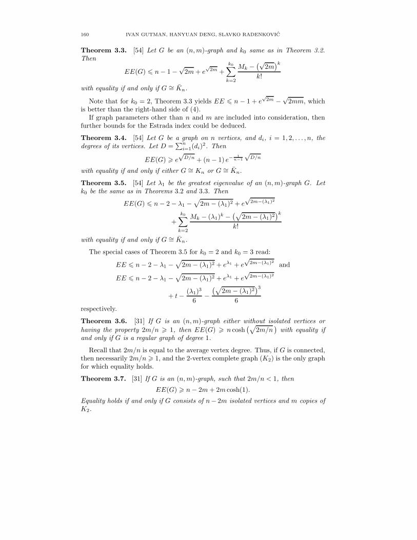
160 IVAN GUTMAN, HANYUAN DENG, SLAVKO RADENKOVIC
Theorem 3.3. [54] Let G be an (n,m)-graph and k0 same as in Theorem 3.2.Then
EE(G) � n− 1−√2m+ e
√2m +
k0∑
k=2
Mk −(√
2m)k
k!
with equality if and only if G ∼= Kn.
Note that for k0 = 2, Theorem 3.3 yields EE � n − 1 + e√2m −√
2mm, whichis better than the right-hand side of (4).
If graph parameters other than n and m are included into consideration, thenfurther bounds for the Estrada index could be deduced.
Theorem 3.4. [54] Let G be a graph on n vertices, and di, i = 1, 2, . . . , n, thedegrees of its vertices. Let D =
∑ni=1(di)
2. Then
EE(G) � e√
D/n + (n− 1) e−1
n−1
√D/n
with equality if and only if either G ∼= Kn or G ∼= Kn.
Theorem 3.5. [54] Let λ1 be the greatest eigenvalue of an (n,m)-graph G. Letk0 be the same as in Theorems 3.2 and 3.3. Then
EE(G) � n− 2− λ1 −√2m− (λ1)2 + e
√2m−(λ1)2
+
k0∑
k=2
Mk − (λ1)k − (√2m− (λ1)2
)k
k!
with equality if and only if G ∼= Kn.
The special cases of Theorem 3.5 for k0 = 2 and k0 = 3 read:
EE � n− 2− λ1 −√2m− (λ1)2 + eλ1 + e
√2m−(λ1)2 and
EE � n− 2− λ1 −√2m− (λ1)2 + eλ1 + e
√2m−(λ1)2
+ t− (λ1)3
6−(√
2m− (λ1)2)3
6respectively.
Theorem 3.6. [31] If G is an (n,m)-graph either without isolated vertices or
having the property 2m/n � 1, then EE(G) � n cosh(√
2m/n)with equality if
and only if G is a regular graph of degree 1.
Recall that 2m/n is equal to the average vertex degree. Thus, if G is connected,then necessarily 2m/n � 1, and the 2-vertex complete graph (K2) is the only graphfor which equality holds.
Theorem 3.7. [31] If G is an (n,m)-graph, such that 2m/n < 1, then
EE(G) � n− 2m+ 2m cosh(1).
Equality holds if and only if G consists of n− 2m isolated vertices and m copies ofK2.

THE ESTRADA INDEX: AN UPDATED SURVEY 161
Theorem 3.8. [31,38] If G is an (n,m)-graph with at least one edge, and if n0 isits nullity, then
EE(G) � n0 + (n− n0) cosh
(√2m
n− n0
).
Equality holds if and only if n− n0 is even, and if G consists of copies of completebipartite graphs Kri,si , i = 1, . . . , (n − n0)/2, such that all products ri · si aremutually equal.
Theorem 3.8 should be compared with inequality (3). It was first proven forbipartite graphs [38] and eventually extended to all graphs. The same result waslater communicated also in [54].
If the graph G is regular of degree r, then its greatest eigenvalue is equal to r. If,in addition, G is bipartite, then its smallest eigenvalue is equal to −r [4]. Bearingthese facts in mind, some of the above bounds could have been simplified [8]:
Theorem 3.9. [8] Let G be a regular graph of degree r and of order n. Then
er +√n+ 2nr − (2r2 + 2r + 1) + (n− 1)(n− 2) e−2r/(n−1)
� EE(G) � n− 2 + er + e√
r(n−r).
The lower bound is improved by including into the consideration also the thirdspectral moment:
EE(G) � er +√n+ 2nr − (2r2+2r+1)+ (n−1)(n−2) e−2r/(n−1) − 4
3 (r3−6t).
Theorem 3.10. [8] Let G be a bipartite regular graph of degree r and of order n.Then
2 cosh(r) +√(n− 2)2 + 2nr − 4 r2
� EE(G) � n− 4 + 2 cosh(r) + 2 cosh(√
nr/2− r2).
In recent works [2, 7] several bounds for the Estrada index were obtained, ofwhich we state here the neat:
Theorem 3.11. [7] Let G be a connected graph with n vertices and m edges.Then,
EE(G) � n+
(2m
n
)2
+1
12
(2m
n
)4
.
4. Estrada indices of some graphs
For graphs whose spectra are known [4], by Eq. (1) one gets explicit expressionsfor their Estrada index. In particular:
EE(Kn) = en−1 + (n− 1) e−1
EE(Ka,n) = a+ b− 2 + 2 cosh(√ab).

162 IVAN GUTMAN, HANYUAN DENG, SLAVKO RADENKOVIC
If Sn is the n-vertex star, then EE(Sn) = n− 2 + 2 cosh(√n− 1
). If Qn is the
hypercube on 2n vertices, then EE(Qn) = [2 cosh(1)]n [24].The (n+1)-vertex wheelWn+1 is obtained by joining a new vertex to each vertex
of the n-vertex cycle Cn. Then EE(Wn+1) = EE(Cn)−e2+2e cosh(√n− 1
)[24].
The Estrada index of the cycle Cn can be approximated as EE(Cn) ≈ n I0, [36]where
I0 =1
π
π∫
0
e2 cosx dx =∞∑
k=0
1
(k!)2= 2.27958530 · · · .
In an analogous manner [26, 36]
EE(Pn) ≈ (n+ 1) I0 − cosh(2)
EE(Zn) ≈ (n+ 2) I0
EE(ZZn) ≈ (n+ 1) I0 + 2 + cosh(2)
where Pn is the n-vertex path, Zn is the (n+ 2)-vertex tree obtained by attachingtwo pendent vertices to a terminal vertex of Pn, whereas ZZn is the (n+4)-vertextree obtained by attaching two pendent vertices to each of the two terminal verticesof Pn.
For positive integers n and m, the tree Pn,m on (m+1)n vertices is obtained byattaching m pendent vertices to each vertex of Pn. Then [26]
EE(Pn,m) ≈ (m− 1)n+ 2(n+ 1)Jm,
where
Jm =1
π
π∫
0
ecosx cosh(√
m+ cos2 x)dx.
Approximations for the Estrada index of Bethe and double-Bethe trees werereported in [52]. Expressions and approximate expressions for EE of several othergraphs can be found in [24].
In [41] the following approximate expression for the Estrada index of an (n,m)-graph was deduced using a Monte Carlo technique:
n(√
6m/n)−1
sinh(√
6m/n)
where sinh stands for the hyperbolic sine [sinh(x) = (ex − e−x)/2]. In [41] alsosome more complicated approximations for EE of (n,m)-graphs were proposed.
4.1. Estrada index of line graphs.
Theorem 4.1. [1] If G is an r-regular graph with n vertices and m = rn/2 edges,and L(G) is its line graph, then EE(L(G)) = er−2EE(G) + (m− n)e−2.
By Theorem 4.1, if G is a connected r-regular graph, then EE(L(G)) = EE(G)holds if and only if r = 1, 2, i.e., if and only if either G ∼= K2 or G ∼= Cn
[24]. To see this, suppose that EE(L(G)) = EE(G) and r � 3. Then m > nand EE(G) = (n − m)/[e2 (er−2 − 1)]. This would imply that EE(G) < 0, acontradiction.

THE ESTRADA INDEX: AN UPDATED SURVEY 163
The k-th iterated line graph Lk(G) of a graphG is defined recursively by Lk(G) =L(Lk−1(G)) where L0(G) ≡ G and L1(G) ≡ L(G).
Theorem 4.2. [1] If G is an r-regular graph with n vertices, and k � 1, then
EE(Lk(G)) = ak(r)EE(G) + bk(r)n
where ak(r) and bk(r) are functions depending solely on the variable r and param-eter k.
In [1] it was shown that ak(r) = e(r−2)(2k−1), which implies ak(r) = O(e(r−2)2k
).
An explicit expression for bk(r) could not be determined, but it was established [1]
that bk(r) has the same asymptotic behavior as ak(r), viz., bk(r) = O(e(r−2)2k
).
4.2. Estrada index of some graph products. Let G and H be two graphs withdisjoint vertex sets. The join G+H of G and H is the graph obtained by connectingall vertices of G with all vertices of H . If G1, G2, . . . , Gn are graphs with mutuallydisjoint vertex sets, then we denote G1 + G2 + · · · + Gn by
∑ni=1Gi. In the case
that G1 = G2 = · · · = Gn = G, we denote∑n
i=1Gi by nG.
Theorem 4.3. [24] Let G and H be r- and s-regular graphs with p and q vertices,respectively. Then
EE(G+H) = EE(G) + EE(H)− (er+ es) + 2e(r+s)/2 cosh(
12
√(r−s)2 + 4pq
).
Corollary 4.4. [24] If G is an r-regular n-vertex graph then
EE(2G) = 2EE(G)− 2er + 2er cosh(n)
EE(3G) = 3EE(G)− 3er + 2er cosh(n) + 2e(2r+n)/2 cosh (3n/2)− er+n.
The Cartesian product G×H of graphs G and H has the vertex set V (G×H)= V (G) × V (H) and (a, x)(b, y) is an edge of G × H if a = b and xy ∈ E(H),or ab ∈ E(G) and x = y. If G1, G2, . . . , Gn are graphs with mutually disjointvertex sets, then we denote G1 × G2 × · · · × Gn by
∏ni=1Gi. In the case that
G1 = G2 = · · · = Gn = G, we denote∏n
i=1Gi by Gn.
Theorem 4.5. [24] EE(G×H) = EE(G)EE(H). More generally,
EE
(r∏
i=1
Gi
)
=r∏
i=1
EE(Gi).
In particular, EE(Gr) = EE(G)r.
5. Graphs with extremal Estrada indices
In [8] de la Pena, Gutman and Rada put forward two conjectures:
Conjecture A. Among n-vertex trees, the path Pn has the minimum and the starSn the maximum Estrada index, i.e., EE(Pn) < EE(Tn) < EE(Sn), where Tn isany n-vertex tree different from Sn and Pn.
Conjecture B. Among connected graphs of order n, the path Pn has the minimumEstrada index.

164 IVAN GUTMAN, HANYUAN DENG, SLAVKO RADENKOVIC
vv vv
v
v
v vv
PS
11 22
3
4
nn
n n
t
... ......
Figure 1. The star Sn and the path Pn, and the labelling of their vertices.
v
v
v v
v v
u(v ) u(v )
v v
1
1
1
2
2
2
3 3
4 4
n n
...
...
G G
G G
I
Figure 2. Transformation I.
In what follows we first state some transformations of graphs and establish therespective change in the spectral moments, and then provide a complete proof ofthese conjectures.
Lemma 5.1. [10] Let Sn be the n-vertex star with vertices v1, v2, . . . , vn, andcenter v1, as shown in Figure 1. Then there is an injection ξ1 from W2k(v2) toW2k(v1), and ξ1 is not surjective for n � 3 and k � 1, where W2k(v1) and W2k(v2)are the sets of self-returning walks of length 2k of v1 and v2 in Sn, respectively.
Proof. Let ξ1 : W2k(v2) → W2k(v1), ∀w ∈ W2k(v2), if w = v2v1vi1 . . . vi2k−3v1v2,
then ξ1(w) = v1v2v1vi1 . . . vi2k−3v1.
Obviously, ξ1 is injective. However, there is no w ∈ W2k(v2) such that
ξ1(w) = v1v3v1v3v1 . . . v3v1 ∈ W2k(v1)
and ξ1 is not surjective for n � 3 and k � 1. �
Lemma 5.2. [10] Consider the Transformation I shown in Figure 2. Let u bea non-isolated vertex of a simple graph G. Let G1 and G2 be the graphs obtainedfrom G by, respectively, identifying a leaf v2 and the center v1 of the n-vertex starSn with the vertex u, cf. Figure 2. Then M2k(G1) < M2k(G2) for n � 3 and k � 2.
Proof. Let W2k(G) denote the set of self-returning walks of length 2k of G. ThenW2k(Gi) =W2k(G)∪W2k(Sn)∪Ai is a partition, where Ai is the set of self-returningwalks of length 2k of Gi, each of them containing both at least one edge in E(G) andat least one edge in E(Sn), i = 1, 2. So, M2k(Gi) = |W2k(G)|+ |W2k(Sn)|+ |Ai| =M2k(G) +M2k(Sn) + |Ai|. Obviously, it is enough to show that |A1| < |A2|.

THE ESTRADA INDEX: AN UPDATED SURVEY 165
Let η1 : A1 → A2, ∀w ∈ A1, η1(w) = (w − w ∩ Sn) ∪ ξ1(w ∩ Sn), i.e., η1(w) isthe self-returning walk of length 2k in A2 obtained from w by replacing its everymaximal (v2, v2)-section in Sn (which is a self-returning walk of v2 in Sn) with itsimage under the map ξ1.
By Lemma 5.1, ξ1 is injective. It is easily shown that η1 is also injective.However, there is no w ∈ A1 such that η1(w) ∈ A2 and η1(w) does not passthe edge v1v2 in G2. So, η1 is not surjective. Consequently, |A1| < |A2| andM2k(G1) < M2k(G2). �
Lemma 5.3. [10] Let Pn = v1v2 . . . vn be the n-vertex path, depicted in Figure 1.Then there is an injection ξ2 from W ′
2k(v1) to W ′2k(vt), and ξ2 is not a surjection
for n � 3, 1 < t < n and k � 1, where W ′2k(v1) and W ′
2k(vt) are the sets ofself-returning walks of length 2k of v1 and vt in Pn, respectively.
Proof. First, let f : {v1, v2, . . . , vt} → {v1, v2, . . . , vt}, f(vi) = vt−i+1 for i =1, 2, . . . , t. Then we can induce a bijection by f from the set of self-returning walksof length 2k of v1 in the sub-path Pt = v1v2 . . . vt and the set of self-returning walksof length 2k of vt in Pt.
Secondly, let ξ2 : W ′2k(v1) →W ′
2k(vt), ∀w ∈ W ′2k(v1).
(i) If w is a walk of Pt = v1v2 . . . vt, i.e., w does not pass the edge vtvt+1, thenξ2(w) = f(w).
(ii) If w passes the edge vtvt+1, we can decompose w into w = w1 ∪ w2 ∪ w3,where w1 is the first (v1, vt)-section of w, w3 is the last (vt, v1)-section of w, andthe rest w2 is the internal maximal (vt, vt)-section of w, i.e., w is a self-returningwalk of v1, first passing the walk w1 from v1 to vt, next passing the walk w2 fromvt to vt, and last passing the walk w3 from vt to v1; then ξ2(w) = w−1
1 ∪w−13 ∪w2,
that is, ξ2(w) is a self-returning walk vt, first passing the reverse of w1 from vt tov1, next passing the reverse of w3 from v1 to vt, and last passing the walk w2 fromvt to vt.
Obviously, ξ2 is injective. And ξ2 is not surjective since there is no w ∈W ′2k(v1)
such that ξ2(w) is a self-returning walk not passing the edge vtvt−1 in Pn of length2k of vt. �
Lemma 5.4. [10] Let u be a non-isolated vertex of a simple graph H. If H1 andH2 are the graphs obtained from H by identifying, respectively, an end vertex v1 andan internal vertex vt of the n-vertex path Pn to u, cf. Figure 3, then M2k(H1) <M2k(H2) for n � 3 and k � 2.
Proof. Let Bi be the set of self-returning walks of length 2k of Hi, each of themcontaining both at least one edge in E(H) and at least one edge in E(Pn), i = 1, 2.Similarly to the proof of Lemma 5.2, it is enough to show that |B1| < |B2|.
Let η2 : B1 → B2, ∀w ∈ B1, η2(w) = (w − w ∩ Pn) ∪ ξ2(w ∩ Pn), i.e., η2(w) isthe self-returning walk of length 2k in B2 obtained from w by replacing its everysection in Pn (which is a self-returning walk of v1 in Pn) with its image under themap ξ2.

166 IVAN GUTMAN, HANYUAN DENG, SLAVKO RADENKOVIC
vv vv
uu
vv vv1
1
1
2
nn tt t+1t+1
...... ......
H H
HHII
Figure 3. Transformation II.
By Lemma 5.3, ξ2 is injective. It follows that η2 is also injective. But, η2 is notsurjective since there is no w ∈ B1 with η2(w) ∈ B2 not passing the edges vtvt−1
in H2. So, |B1| < |B2|. �
Theorem 5.5. [10] If Tn is a n-vertex tree different from Sn and Pn, then
(12) EE(Pn) < EE(Tn) < EE(Sn).
Proof. Repeating Transformation I, as shown in Figure 2, any n-vertex tree T canbe changed into the n-vertex star Sn. By Lemma 5.2, we have M2k(T ) < M2k(Sn)for k � 2. This implies
EE(T ) =∑
k�0
M2k(T )
(2k)!<∑
k�0
M2k(Sn)
(2k)!= EE(Sn).
On the other hand, repeating Transformation II, as shown in Figure 3, any n-vertex tree T can be changed into the n-vertex path Pn. By Lemma 5.4, we haveM2k(T ) > M2k(Pn) for k � 2. Consequently,
EE(T ) =∑
k�0
M2k(T )
(2k)!>∑
k�0
M2k(Pn)
(2k)!= EE(Pn).
So the inequalities (12) hold. �
Theorem 5.5 shows that the path Pn and the star Sn have the minimum and themaximum Estrada indices among n-vertex trees, i.e., Conjecture A is true.
Zhao and Jia [53] have determined also the trees with the second and the thirdgreatest Estrada index. In fact, they proved:
Theorem 5.6. [53] Let S1n∼= Sn be the n-vertex star, cf. Figure 1, and let the
n-vertex trees Sin, i = 2, 3, 4, 5, 6, be those shown in Figure 4. Let T1 and T2 be
n-vertex trees, such that T1 /∈ {Sin | i = 1, 2, 3, 4, 5, 6} and T2 /∈ {Si
n | i = 1, 2, 3}.Then for n � 6,
EE(S1n) > EE(S2
n) > EE(S3n) > EE(S5
n) > EE(S6n) > EE(T1)
and
EE(S1n) > EE(S2
n) > EE(S3n) > EE(T2).
Consequently, among n-vertex trees, the first three trees with the greatest Estradaindices are Sn, S
2n and S3
n, respectively.

THE ESTRADA INDEX: AN UPDATED SURVEY 167
S
S
S
S
S
n
n
n
n
n
......
...
......
{
{
{
{
{
n-3
n-5
n-5
n-4
n-4
2
4
6
3
5
Figure 4. The graphs Sin, i = 2, 3, 4, 5, 6, having the second,
third, fourth, fifth, and sixth greatest Estrada indices among n-vertex trees [11, 53].
Recently it was demonstrated [11] that EE(S3n) > EE(S4
n) > EE(S5n), from
which follows:
Theorem 5.7. [11] Among n-vertex trees, n � 6, the first six trees with thegreatest Estrada indices are Sn, S
2n, S
3n, S
4n, S
5n, S
6n, respectively, cf. Figure 4.
Theorem 5.5 can be extended also in another way. Denote by Bn,Δ the treeobtained by attaching Δ − 1 pendent vertices to a pendent vertex of the pathPn−Δ+1. This tree is usually referred to as a “broom” (cf. [9]).
Theorem 5.8. [42] Among all trees on n vertices and maximum vertex degree Δ,the broom Bn,Δ has minimum Estrada index.
Theorem 5.9. [42] Observing that Bn,n−1 ≡ Sn and Bn,2 ≡ Pn, we have
EE(Bn,n−1) > EE(Bn,n−2) > · · · > EE(Bn,3) > EE(Bn,2).
Let G be a connected graph of order n and let e be an edge of G. The graphG′ = G−e is obtained from G by deleting the edge e. Obviously, any self-returningwalk of length k of G′ is also a self-returning walk of length k of G. Thus,
Mk(G′) �Mk(G) and EE(G′) � EE(G).
In particular, if T is a spanning tree of G, then
Mk(T ) �Mk(G) and EE(T ) � EE(G).
From Theorem 5.5 it follows that EE(Pn) � EE(G). So, we have:
Theorem 5.10. [10] If G is a simple connected graph of order n different fromthe complete graph Kn and the path Pn, then
EE(Pn) < EE(G) < EE(Kn).

168 IVAN GUTMAN, HANYUAN DENG, SLAVKO RADENKOVIC
Theorem 5.10 shows that the path Pn and the complete graph Kn have theminimum and the maximum Estrada indices among connected graphs of order n,i.e., Conjecture B is true.
Independently of the work of one of the present author [10, 11], Das and Leealso examined the Conjectures A and B [7]. For any connected (n,m)-graph G,they were able to show that EE(G) > EE(Pn) provided m � 1.8n+ 4, and thatEE(G) � E(Pn) provided m � n2/6. In addition, they also proved that amongtrees, the star has maximum Estrada index.
6. Estrada indices of molecular graphs
In view of the chemical origin of the Estrada index, it is natural than moleculargraphs [37], especially acyclic and benzenoid, were among the first whose structure–dependence was systematically examined.
Figure 5. Correlation between the Estrada indices and the pa-rameter D (= sum of squares of vertex degrees) for the 106 treeson 10 vertices.
A chemical tree is a tree in which no vertex has degree greater than four [37].Among the n-vertex chemical trees, Pn has minimum Estrada index. For theEstrada index of chemical trees it was concluded [35] that the n-vertex chemicaltree with the greatest Estrada index might be the Volkmann tree V Tn(4). However,this assertion cannot be considered as proven in a rigorous mathematical manner.Such a proof awaits to be achieved in the future.
In the case of trees with a fixed number of vertices (including both chemicaland non-chemical trees) it was found that EE increases with the increasing extentof branching [34]. This fact motivated investigations of the relation between EE

THE ESTRADA INDEX: AN UPDATED SURVEY 169
Figure 6. Correlation between the Estrada index (EE) and thegreatest graph eigenvalue λ1 for the 106 trees on 10 vertices.
and other branching indices. It was established that there is a linear correlationbetween EE and the quantity D =
∑ni=1(di)
2, earlier encountered in Theorem 3.4,see Figure 5.
The quantitative analysis of these correlations resulted in the following approx-imate expression:
EE ≈ 1.735n− 0.13 + 0.11D.
This formula is capable of reproducing EE with an error less than 0.1%.The Estrada index of trees was also correlated with the greatest graph eigenvalue
[35,40]; a characteristic example of such correlations is shown in Figure 6. One cansee that the EE/λ1 relation is not simple. The fact that the (EE, λ1) data pointsare grouped on several (almost) horizontal lines indicates that EE is much lesssensitive to structural features than λ1.
Empirical studies revealed that the number of vertices n and number of edgesm are the main factors influencing EE-value of molecular graphs [34, 39, 41]. Forbenzenoid systems, (m,n)-type approximations are capable of reproducing over99.8% of EE-value [39, 41]. In order to find some finer structural details on whichEE depends, series of isomeric benzenoid systems (having equal n and m) wereexamined. The Estrada indices of benzenoid isomers vary only to a very limitedextent. The main structural feature influencing these variations is the number ofbay regions, b. (The quantity b is equal to the number of edges on the boundary ofa benzenoid graph, connecting two vertices of degree 3; for details see [32].) Withinsets of benzenoid isomers, EE is an increasing linear function of b, see Figure 7.
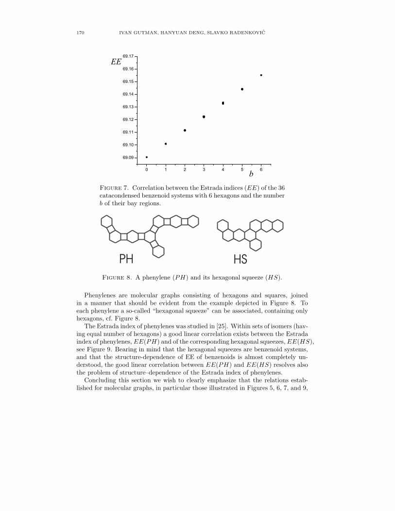
170 IVAN GUTMAN, HANYUAN DENG, SLAVKO RADENKOVIC
Figure 7. Correlation between the Estrada indices (EE) of the 36catacondensed benzenoid systems with 6 hexagons and the numberb of their bay regions.
PH HS
Figure 8. A phenylene (PH) and its hexagonal squeeze (HS).
Phenylenes are molecular graphs consisting of hexagons and squares, joinedin a manner that should be evident from the example depicted in Figure 8. Toeach phenylene a so-called “hexagonal squeeze” can be associated, containing onlyhexagons, cf. Figure 8.
The Estrada index of phenylenes was studied in [25]. Within sets of isomers (hav-ing equal number of hexagons) a good linear correlation exists between the Estradaindex of phenylenes, EE(PH) and of the corresponding hexagonal squeezes, EE(HS),see Figure 9. Bearing in mind that the hexagonal squeezes are benzenoid systems,and that the structure-dependence of EE of benzenoids is almost completely un-derstood, the good linear correlation between EE(PH) and EE(HS) resolves alsothe problem of structure–dependence of the Estrada index of phenylenes.
Concluding this section we wish to clearly emphasize that the relations estab-lished for molecular graphs, in particular those illustrated in Figures 5, 6, 7, and 9,
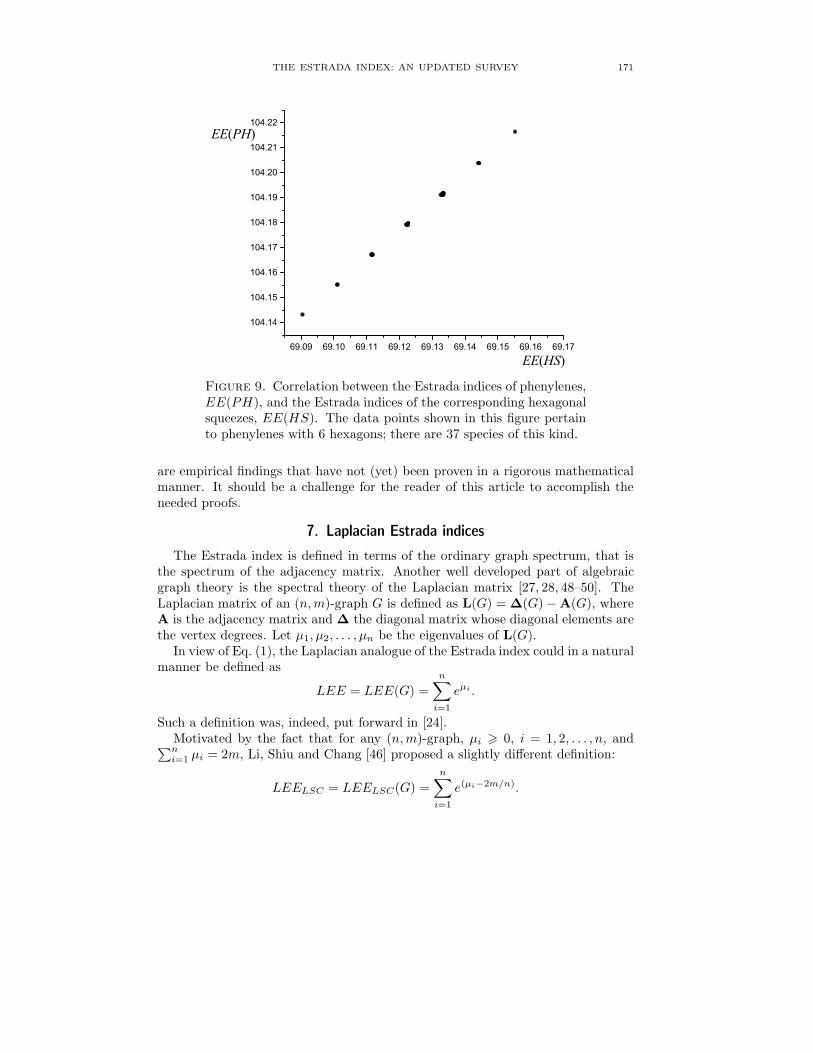
THE ESTRADA INDEX: AN UPDATED SURVEY 171
Figure 9. Correlation between the Estrada indices of phenylenes,EE(PH), and the Estrada indices of the corresponding hexagonalsqueezes, EE(HS). The data points shown in this figure pertainto phenylenes with 6 hexagons; there are 37 species of this kind.
are empirical findings that have not (yet) been proven in a rigorous mathematicalmanner. It should be a challenge for the reader of this article to accomplish theneeded proofs.
7. Laplacian Estrada indices
The Estrada index is defined in terms of the ordinary graph spectrum, that isthe spectrum of the adjacency matrix. Another well developed part of algebraicgraph theory is the spectral theory of the Laplacian matrix [27, 28, 48–50]. TheLaplacian matrix of an (n,m)-graph G is defined as L(G) = Δ(G)−A(G), whereA is the adjacency matrix and Δ the diagonal matrix whose diagonal elements arethe vertex degrees. Let μ1, μ2, . . . , μn be the eigenvalues of L(G).
In view of Eq. (1), the Laplacian analogue of the Estrada index could in a naturalmanner be defined as
LEE = LEE(G) =
n∑
i=1
eμi .
Such a definition was, indeed, put forward in [24].Motivated by the fact that for any (n,m)-graph, μi � 0, i = 1, 2, . . . , n, and∑ni=1 μi = 2m, Li, Shiu and Chang [46] proposed a slightly different definition:
LEELSC = LEELSC(G) =
n∑
i=1
e(μi−2m/n).

172 IVAN GUTMAN, HANYUAN DENG, SLAVKO RADENKOVIC
Evidently,LEELSC(G) = e−2m/nEE(G)
and therefore it is no surprise that the lower and upper bounds for LEE obtainedin [56] and those for LEELSC obtained in [46] were found to be equivalent. Morebounds for LEE were reported in [2, 55].
Generally speaking, the Laplacian Estrada index has properties closely analogousto those of the ordinary Estrada index. Thus, we have:
Theorem 7.1. [43] If Tn is a n-vertex tree different from Sn and Pn, then
LEE(Pn) < LEE(Tn) < LEE(Sn).
This result is fully analogous to Theorem 5.5.In [43] also the n-vertex tree with second-maximal Laplacian Estrada index was
characterized. Denote by Sn(a, b) the tree formed by adding an edge between thecenters of the stars Sa and Sb, in which case n = a+ b. This tree is called a “doublestar”.
Theorem 7.2. [43] For n � 4, the unique n-vertex tree with second-maximalLaplacian Estrada index is Sn(2, n− 2).
One of the present authors together with Jie Zhang could promptly improveTheorem 7.2:
Theorem 7.3. [13] For n � 6, the n-vertex tree with third-maximal LaplacianEstrada index is Sn(3, n− 3).
Among results that relate the Laplacian Estrada index with the ordinary Estradaindex we point out the trivial:
Theorem 7.4. If G is a regular graph of degree r, then LEE(G) = er EE(G).
and the less straightforward:
Theorem 7.5. [56] If G is a bipartite (n,m)-graph, then LEE(G) = n − m +e2EE(L(G)), where L(G) is the line graph of G.
Concluding this section we mention that also the distance Estrada index wasrecently considered [29], in which instead of eigenvalues of the adjacency matrixone used the eigenvalues of the distance matrix.
References
[1] T. Aleksic, I. Gutman, M. Petrovic, Estrada index of iterated line graphs, Bull. Acad. SerbeSci. Arts (Cl. Sci. Math. Natur.) 134 (2007), 33–41.
[2] H. Bamdad, F. Ashraf, I. Gutman, Lower bounds for Estrada index and Laplacian Estradaindex, Appl. Math. Lett. textbf23 (2010), 739–742.
[3] R. Carbo–Dorca, Smooth function topological structure descriptors based on graph–spectra,J. Math. Chem. 44 (2008), 373–378.
[4] D. Cvetkovic, M. Doob, H. Sachs, Spectra of Graphs – Theory and Application, third ed.,Johann Ambrosius Barth Verlag, Heidelberg, Leipzig, 1995.
[5] D. Cvetkovic, P. Rowlinson, S. Simic, An Introduction to the Theory of Graph Spectra,Cambridge Univ. Press, Cambridge, 2010.

THE ESTRADA INDEX: AN UPDATED SURVEY 173
[6] L. Da Fontoura Costa, M.A.R. Tognetti, F. N. Silva, Concentric characterization and clas-sification of complex network nodes: Application to an institutional collaboration network,Physica A387 (2008), 6201–6214.
[7] K.C. Das, S. G. Lee, On the Estrada index conjecture, Lin. Algebra Appl. 431 (2009), 1351–1359.
[8] J. A. de la Pena, I. Gutman, J. Rada, Estimating the Estrada index, Lin. Algebra Appl. 427(2007), 70–76.
[9] R.R. del Vecchio, I. Gutman, V. Trevisan, C.T.M. Vinagre, On the spectra and energies ofdouble–broom–like trees, Kragujevac J. Sci. 31 (2009), 45–58.
[10] H. Deng, A proof of a conjecture on the Estrada index, MATCH Commun. Math. Comput.Chem. 62 (2009), 599–606.
[11] H. Deng, A note on the Estrada index of trees, MATCH Commun. Math. Comput. Chem.62 (2009), 607–610.
[12] H. Deng, S. Radenkovic, I. Gutman, The Estrada index, in: D. Cvetkovic, I. Gutman, Eds.Applications of Graph Spectra, Math. Inst., Belgrade, 2009, pp. 123–140.
[13] H. Deng, J. Zhang, A note on the Laplacian Estrada index of trees, MATCH Commun. Math.Comput. Chem. 63 (2010), 777–782.
[14] T. Doslic, Bipartiviy of fullerene graphs and fullerene stability, Chem. Phys. Lett. 412 (2005),336–340.
[15] E. Estrada, Characterization of 3D molecular structure, Chem. Phys. Lett. 319 (2000), 713–718.
[16] E. Estrada, Characterization of the folding degree of proteins, Bioinformatics 18 (2002),697–704.
[17] E. Estrada, Characterization of the amino acid contribution to the folding degree of proteins,Proteins 54 (2004), 727–737.
[18] E. Estrada, Topological structural classes of complex networks, Phys. Rev. E 75 (2007),016103.
[19] E. Estrada, Atom–bond connectivity and the energetic of branched alkanes, Chem. Phys.Lett. 463 (2008), 422–425.
[20] E. Estrada, N. Hatano, Statistical–mechanical approach to subgraph centrality in complexnetworks, Chem. Phys. Lett. 439 (2007), 247–251.
[21] E. Estrada, J. A. Rodrıguez–Velazquez, Subgraph centrality in complex networks, Phys. Rev.E 71 (2005), 056103.
[22] E. Estrada, J. A. Rodrıguez–Velazquez, Spectral measures of bipartivity in complex networks,Phys. Rev. E 72 (2005), 046105.
[23] E. Estrada, J.A. Rodrıguez–Velazquez, M. Randic, Atomic branching in molecules, Int. J.
Quantum Chem. 106 (2006), 823–832.[24] G.H. Fath-Tabar, A.R. Ashrafi, I. Gutman, Note on Estrada and L-Estrada indices of graphs,
Bull. Acad. Serbe Sci. Arts. (Cl. Math. Natur.) 139 (2009), 1–16.[25] B. Furtula, I. Gutman, Energy and Estrada index of phenylenes, Indian J. Chem. 47A (2008),
220–224.[26] Y. Ginosar, I. Gutman, T. Mansour, M. Schork, Estrada index and Chebyshev polynomials,
Chem. Phys. Lett. 454 (2008), 145–147.[27] R. Grone, R. Merris, The Laplacian spectrum of a graph II, SIAM J. Discr. Math. 7 (1994),
221–229.[28] R. Grone, R. Merris, V. S. Sunder, The Laplacian spectrum of a graph, SIAM J. Matrix Anal.
Appl. 11 (1990), 218–238.[29] A. D. Gungor, S. B. Bozkurt, On the distance Estrada index of graphs, Hacettepe J. Math.
Statist. 38 (2009), 277–283.[30] A. Gursoy, O. Keskin, R. Nussinov, Topological properties of protein interaction networks
from a structural perspective, Biochem. Soc. Trans. 36 (2008), 1398–1403.[31] I. Gutman, Lower bounds for Estrada index, Publ. Inst. Math. (Beograd), 83 (2008), 1–7.

174 IVAN GUTMAN, HANYUAN DENG, SLAVKO RADENKOVIC
[32] I. Gutman, S. J. Cyvin, Introduction to the Theory of Benzenoid Hydrocarbons, Springer–Verlag, Berlin, 1989.
[33] I. Gutman, E. Estrada, J.A. Rodrıguez–Velazquez, On a graph–spectrum–based structuredescriptor, Croat. Chem. Acta 80 (2007), 151–154.
[34] I. Gutman, B. Furtula, B. Glisic, V. Markovic, A. Vesel, Estrada index of acyclic molecules,Indian J. Chem. 46 (2007), 723–728.
[35] I. Gutman, B. Furtula, V. Markovic, B. Glisic, Alkanes with greatest Estrada index, Z.Naturforsch. 62a (2007), 495–498.
[36] I. Gutman, A. Graovac, Estrada index of cycles and paths, Chem. Phys. Lett. 436 (2007),294–296.
[37] I. Gutman, O. E. Polansky, Mathematical Concepts in Organic Chemistry, Springer–Verlag,Berlin, 1986.
[38] I. Gutman, S. Radenkovic, A lower bound for the Estrada index of bipartite molecular graphs,Kragujevac J. Sci. 29 (2007), 67–72.
[39] I. Gutman, S. Radenkovic, Estrada index of benzenoid hydrocarbons, Z. Naturforsch. 62a(2007), 254–258.
[40] I. Gutman, S. Radenkovic, B. Furtula, T. Mansour, M. Schork, Relating Estrada index withspectral radius, J. Serb. Chem. Soc. 72 (2007), 1321–1327.
[41] I. Gutman, S. Radenkovic, A. Graovac, D. Plavsic, Monte Carlo approach to Estrada index,Chem. Phys. Lett. 446 (2007), 233–236.
[42] A. Ilic, D. Stevanovic, The Estrada index of chemical trees, J. Math. Chem. 47 (2010),305–314.
[43] A. Ilic, B. Zhou, Laplacian Estrada index of trees, MATCH Commun. Math. Comput. Chem.63 (2010), 769–776.
[44] M. Jungsbluth, B. Burghardt, A.K. Hartmann, Fingerprinting networks: Correlations oflocal and global network properties, Physica A381 (2007), 444–456.
[45] V.V. Kerrenbroeck, E. Marinari, Ranking vertices or edges of a network by loops: A newapproach, Phys. Rev. Lett. 101 (2008), 098701.
[46] J. Li, W.C. Shiu, A. Chang, On Laplacian Estrada index of a graph, Appl. Anal. Discr.Math. 3 (2009), 147–156.
[47] C.Y. Lin, C. H. Chin, H.H. Wu, S.H. Chen, C.W. Ho, M.T. Ko, HUBBA: Hubs objectsanalyzer – a framework of interactome hubs identification for network biology, Nucleic AcidsRes. 36 (2008), 438–443.
[48] R. Merris, Laplacian matrices of graphs: A survey, Lin. Algebra Appl. 197–198 (1994),143–176.
[49] R. Merris, A survey of graph Laplacians, Lin. Multilin. Algebra 39 (1995), 19–31.
[50] B. Mohar, The Laplacian spectrum of graphs, in: Y. Alavi, G. Chartrand, O. R. Oellermann,A. J. Schwenk, Eds. Graph Theory, Combinatorics, and Applications, Wiley, New York, 1991,pp. 871–898.
[51] A. Platzer, P. Perco, A. Lukas, B. Mayer, Characterization of protein–interaction networksin tumors, BMC Bioinformatics 8 (2007), 224–229.
[52] M. Robbiano, R. Jimenez, L. Medina, The energy and an approximation to Estrada index ofsome trees, MATCH Commun. Math. Comput. Chem. 61 (2009), 369–382.
[53] H. Zhao, Y. Jia, On the Estrada index of bipartite graphs, MATCH Commun. Math. Comput.Chem. 61 (2009), 495–501.
[54] B. Zhou, On Estrada index, MATCH Commun. Math. Comput. Chem. 60 (2008), 485–492.[55] B. Zhou, On sum of powers of Laplacian eigenvalues and Laplacian Estrada index of graphs,
MATCH Commun. Math. Comput. Chem. 62 (2009), 611–619.[56] B. Zhou, I. Gutman, More on the Laplacian Estrada index, Appl. Anal. Discr. Math. 3
(2009), 371–378.[57] E. Zotenko, J. Mestre, D.P. O’Leary, T.M. Przytycka, Why do hubs in the yeast protein
interaction network tend to be essential: Re-examining the connection between the networktopology and essentiality, Computat. Biol. 4 (2008), 1–16.