Spectral Graph Theory

Outline:

• Definitions and different spectra

• Physical analogy

• Description of bisection algorithm

• Relationship of spectrum to graph structure

• My own recent work on graphical images

I. Definition and Different Spectra:

• Spectrum: The set of eigenvalues corresponding to a matrix

• Two major kinds of graph matricies used in this context: Adjacency and Laplacian

Adjacency Matrix

If graph is undirected, A is symmetric. This means that its eigenvectors are real and orthogonal

Laplacian MatrixLet D be the matrix composed of I multiplied by a vector containing the degree of each vertex

Then,

Sometimes normalized by

Spectra Intuition

• For each vertex, assign a number so that the number is proportional to the sum of all its neighbor’s numbers: Proportions are eigenvalues of A

• For each vertex, assign a number so that the number is proportional to the difference between of all its neighbor’s numbers and itself multiplied by its degree: Proportions are eigenvalues of L

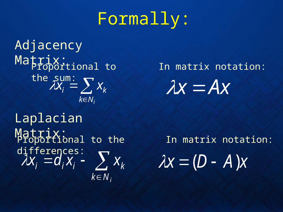
Formally:

In matrix notation:Proportional to the sum:

Adjacency Matrix:

In matrix notation:Proportional to the differences:

Laplacian Matrix:

II. Physical Analogies

• Harmonic modes of a vibrating string

• Chemistry: Hückel theory showed that the spectra of a molecule’s adjacency matrix is related to the energy of the corresponding molecular orbitals

Modes of a string

x1

x2

x3

x4

x5

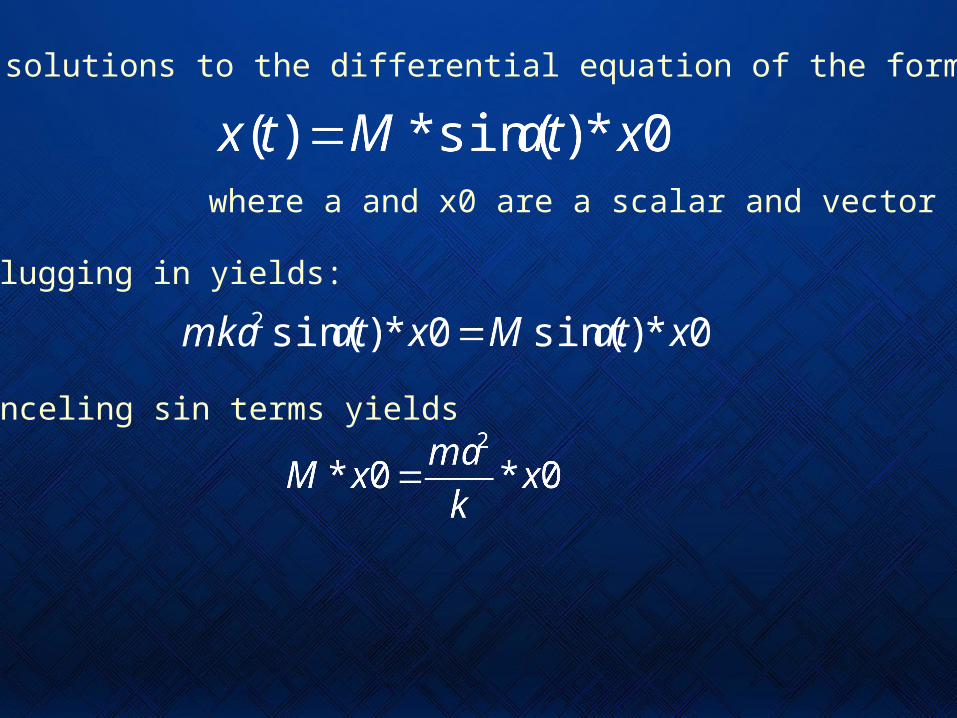
Seeking solutions to the differential equation of the form:

Plugging in yields:

Canceling sin terms yields

where a and x0 are a scalar and vector

Therefore eigenvalues of M are:

With eigenvectors:

Modes of a string concluded

• Therefore the eigenvectors of the Laplacian form the harmonic basis set with coefficients equal to the eigenvalues

• Demmel suggests that harmonic analogy works in 2D, giving “fault lines” in the surface

III. Spectral bisection algorithm

• Builds L, finds the eigenvector corresponding to the second smallest eigenvalue (Fiedler value) and partitions nodes based on a cut point in the corresponding eigenvector (Fiedler vector)

Rationale behind method

• Since rows/colums all add to zero in L, the first eigenvector will be all ones and the first eigenvalue will be zero

• Second eigenvalue/eigenvector known as the Fiedler vector/value

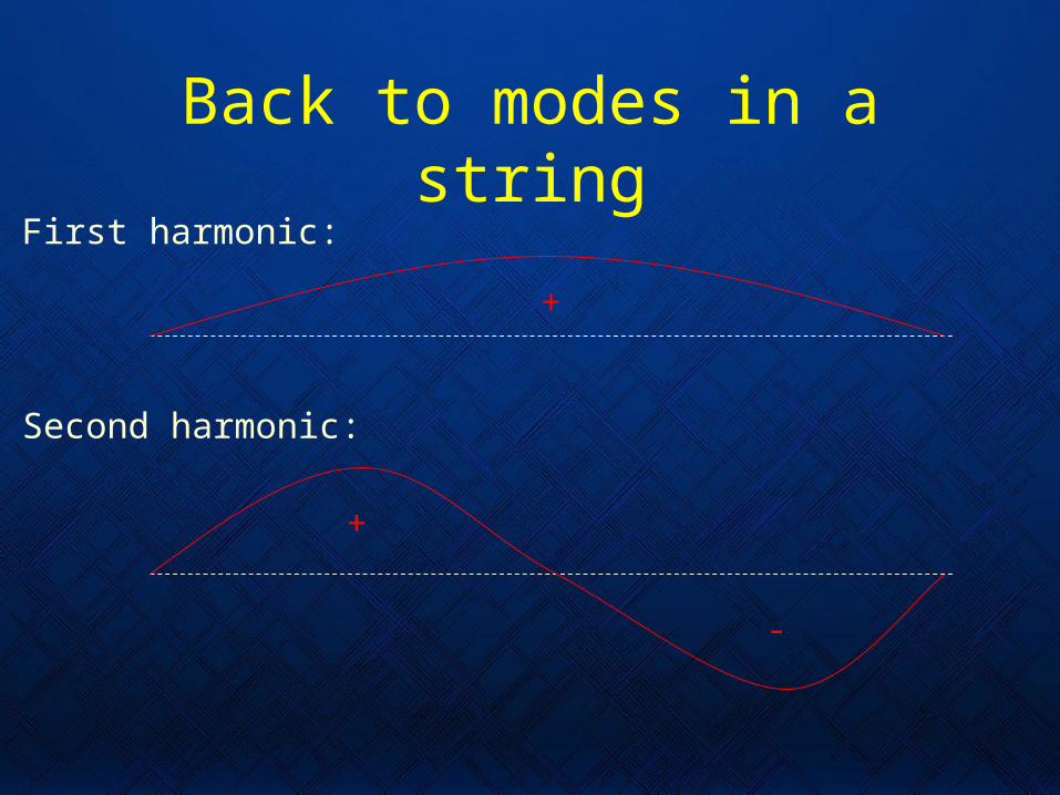
Back to modes in a string

+

First harmonic:

Second harmonic:

+

-

Possible choices of a cut-point• Median cut: Use median value in

eigenvector

• Ratio cut: Use point which gives the best ratio of vertices separated to edges cut

• Sign cut: Cut-point equals zero

• Gap cut: Choose value at largest gap in the sorted list of Fiedler vector components

Demmel endorses sign cut, most applied researchers seem to favor median cut, while mathematicians (and Shi/Malik) favor ratio cut

Q. How to approximate eigenvalues/vectors of a sparse, symmetric matrix?

A. The Lanczos method

Lanczos method takes an n x n sparse, symmetric matrix A and computes a k x k tridiagonal matrix T whose eigenvalues/vectors are good approximations of those in A

Even with k much smaller than n, the approximation is fairly good. Fortunately, the values which converge first are the largest and smallest, including the Fiedler values

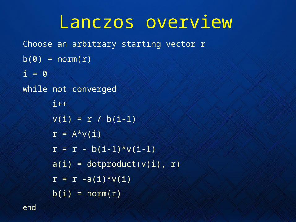
Lanczos overviewChoose an arbitrary starting vector r

b(0) = norm(r)

i = 0

while not converged

i++

v(i) = r / b(i-1)

r = A*v(i)

r = r - b(i-1)*v(i-1)

a(i) = dotproduct(v(i), r)

r = r -a(i)*v(i)

b(i) = norm(r)

end

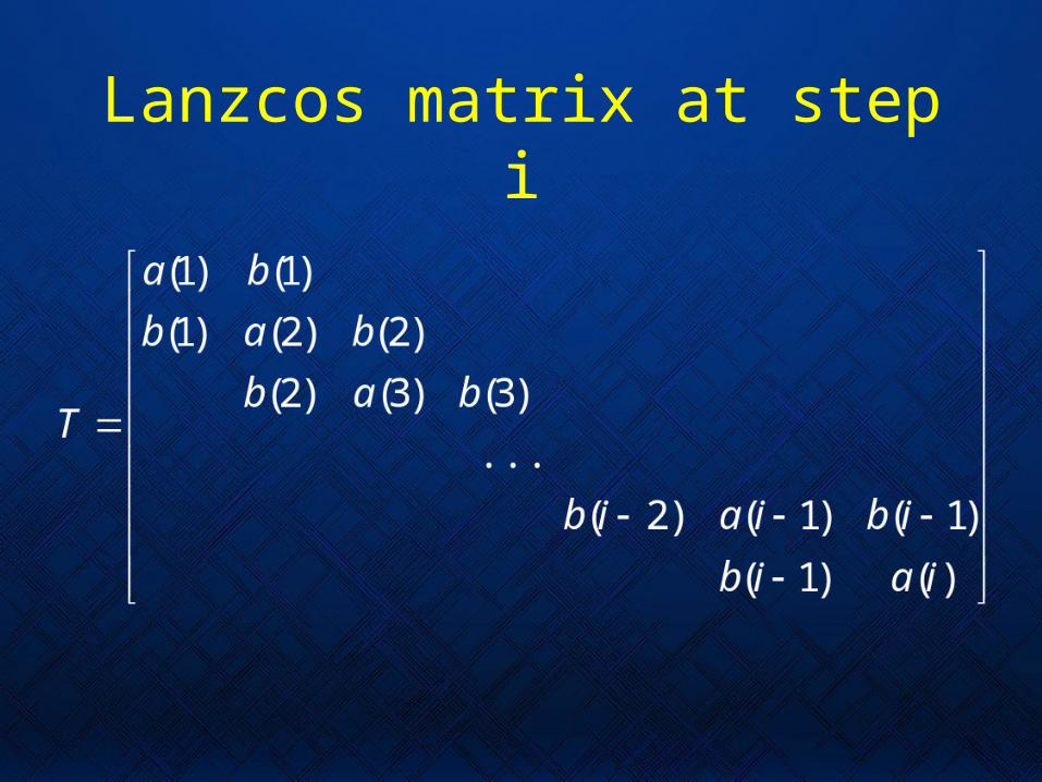
Lanzcos matrix at step i

Problem: Lanczos method too slowSolution: Multilevel method

• Coarsen using MIS

• Find eigenvectors of coarsened graph using Rayleigh Quotient Iteration (RQI)

• Project eigenvectors back to original graph using coarsened values to seed RQI

Although approximation is quick and dirty, when you’re only concerned with the sign (or median or...), a rough approximation is okay

IV. Beyond partitioning: Structural relationships

• Knowing the spectrum of a graph can tell you certain things about the graph’s structure and visa versa

Isomorphisms

• Cospectral graphs are not necessarily isomorphic, but isomorphic graphs are always cospectral

• Spectrum is invariant to nonsingular transformations (e.g. permutations, affine transforms, etc.)

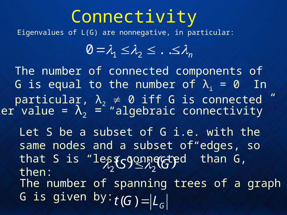
ConnectivityEigenvalues of L(G) are nonnegative, in particular:

The number of connected components of G is equal to the number of λi = 0 In particular, λ2 0 iff G is connected

Feidler value = λ2 = “algebraic connectivity”

Let S be a subset of G i.e. with the same nodes and a subset of edges, so that S is “less connected” than G, then:

The number of spanning trees of a graph G is given by:

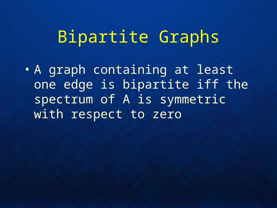
Bipartite Graphs

• A graph containing at least one edge is bipartite iff the spectrum of A is symmetric with respect to zero

Cheeger constantsFor a subset of the vertices S, let:

Define the Cheeger constant as:

Then the Fiedler value is bounded by:

Regularity

A graph is regular with degree r iff:

Conclusion

• Graph spectra have many curious and surprising relationships to graph structure

• Many more theorems related to graph spectra

• Most work focuses either on applications or proving various bounds on the values

Current Work in Image Processing

Build a graph-based IP environment

• Problem definition

• Data structure

• Resolved issues

• Current IP routines

• Future directions

Problem: Liberate IP from pixels

Solution: Formulate IP on graphs

Advantages:

Space variant vision possible

Processing on fewer components in same domain

Graph algorithms are fast

Goals:

Space variant applications

Choosing nodes based on content

Use graph theory algorithms to novel ends

Logonoid simulations, etc.

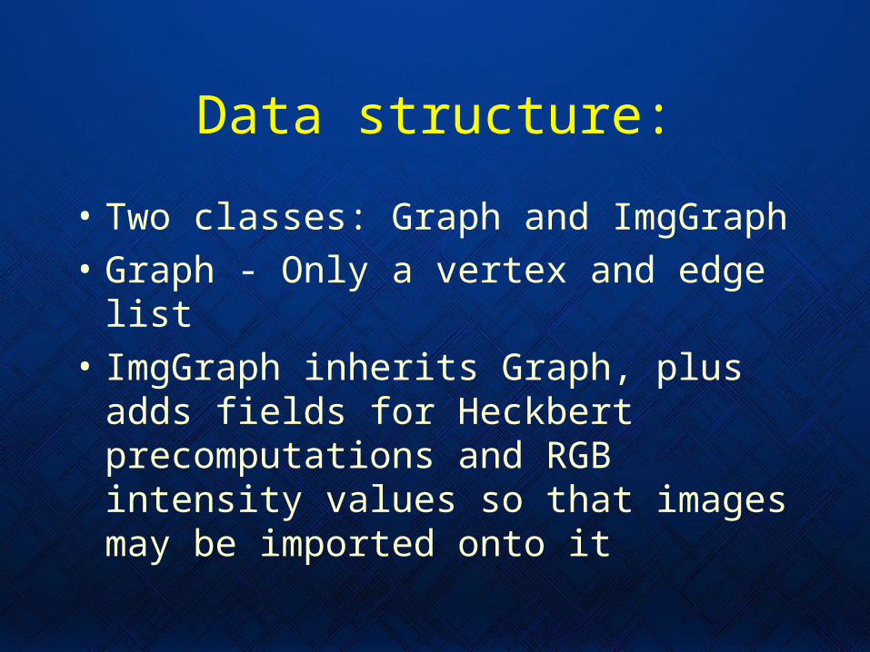
Data structure:

• Two classes: Graph and ImgGraph

• Graph - Only a vertex and edge list

• ImgGraph inherits Graph, plus adds fields for Heckbert precomputations and RGB intensity values so that images may be imported onto it

What’s not in the structure:• Neighbor list (i.e. flowers)

• Edge weights

• Face list (more on this later)

Why?All of these fields aren’t necessary for many methods (i.e. face list is only necessary if visualizing), leading to possibly unneeded:

• Precomputation time

• Storage space

• Updating (e.g. when deleting nodes/edges)

Current methods - Graph

• Get/set - Basic OOP methods

• Neighborhood - Compute neighbor list and distances to each neighbor

• Removeedge - Removes an edge

• Removenode - Remove a node

Current methods - ImgGraphGet/set - Basic OOP methods

Adjacency - Computes the adjacency matrix

Laplacian - Computes the Laplacian matrix

Impotimg - Imports an image centered at location fovea

Edgegraph - Computes the edge map using 1st derivative

Makeweights - Computes edge weights

Neighborhood - Compute neighbor list and distances to each neighbor

Removenode - Removes a node list

Removeisolated - Finds and removes nodes of degree zero

Threshcut - Segmentation by intensity thresholding

Showstruct -Displays graph structure without image data

Showmesh - Displays graph by interpolating across enclosed polygons

Showgraph - Displays graph as a traditional stick-and-ball, where balls are colored to reflect RGB values at the node

Findfaces - Generates a list of enclosed polygons that can be fed to patch in the Showmesh call

Problems to solve

• Importing images

• Assigning edge weights

• Visualization

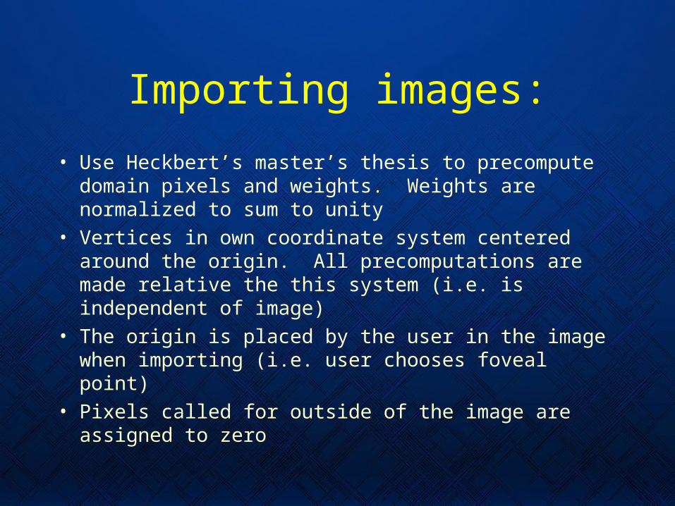
Importing images:

• Use Heckbert’s master’s thesis to precompute domain pixels and weights. Weights are normalized to sum to unity

• Vertices in own coordinate system centered around the origin. All precomputations are made relative the this system (i.e. is independent of image)

• The origin is placed by the user in the image when importing (i.e. user chooses foveal point)

• Pixels called for outside of the image are assigned to zero

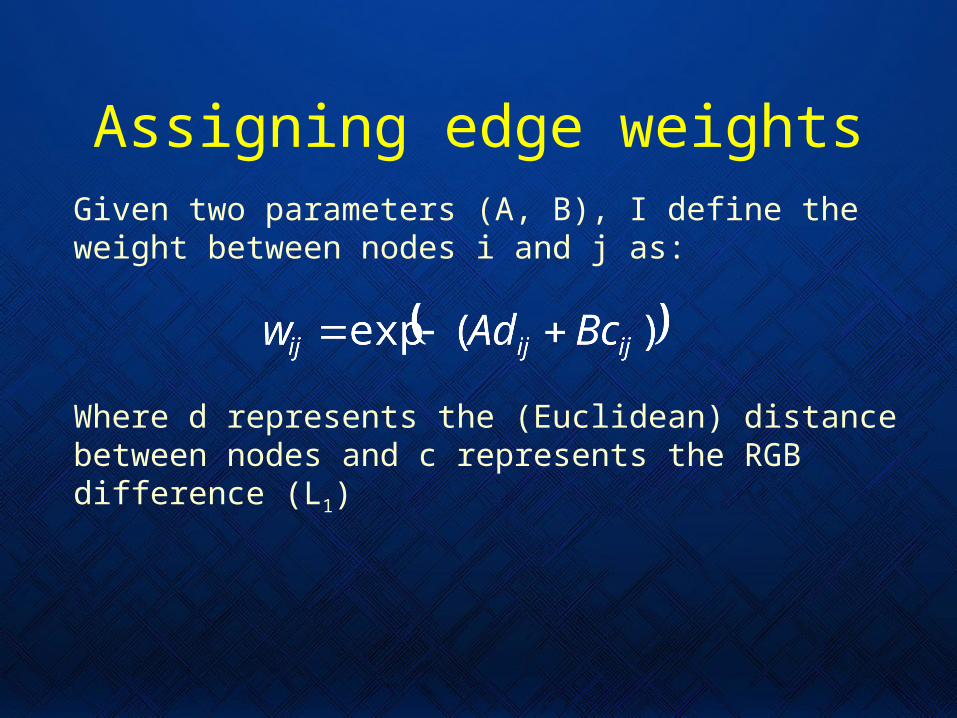
Assigning edge weightsGiven two parameters (A, B), I define the weight between nodes i and j as:

Where d represents the (Euclidean) distance between nodes and c represents the RGB difference (L1)

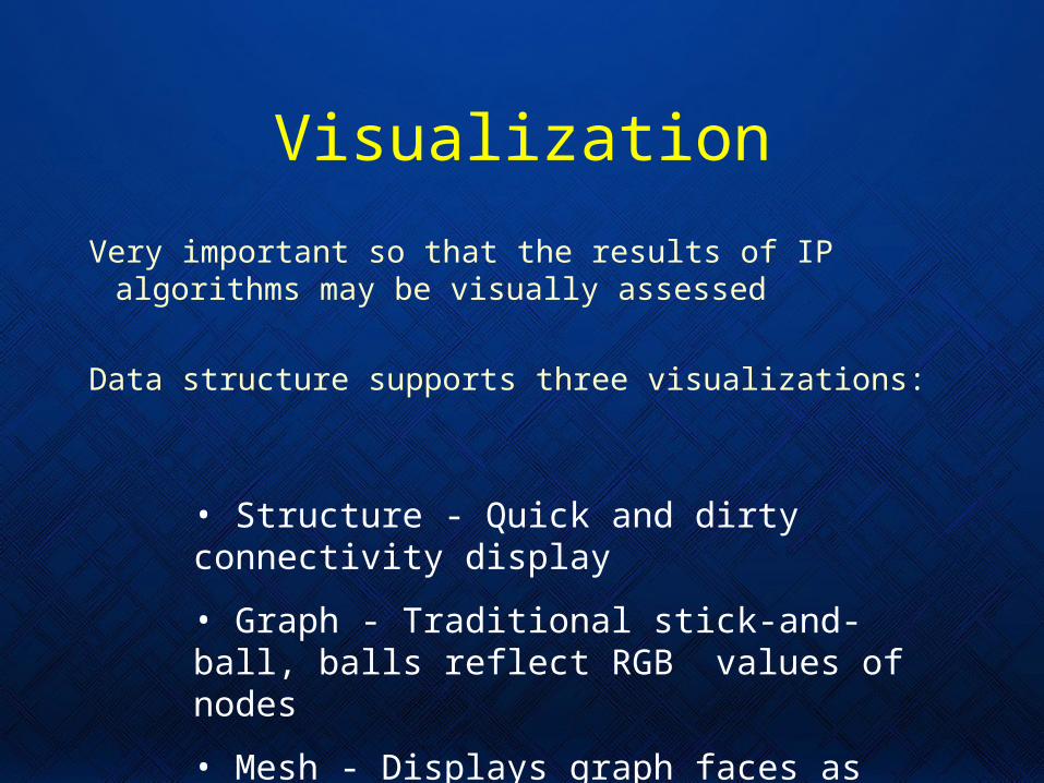
Visualization

Very important so that the results of IP algorithms may be visually assessed

Data structure supports three visualizations:

• Structure - Quick and dirty connectivity display

• Graph - Traditional stick-and-ball, balls reflect RGB values of nodes

• Mesh - Displays graph faces as filled-in polygons

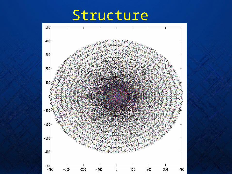
Structure

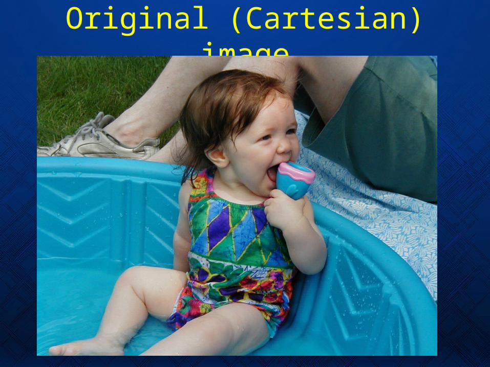
Original (Cartesian) image

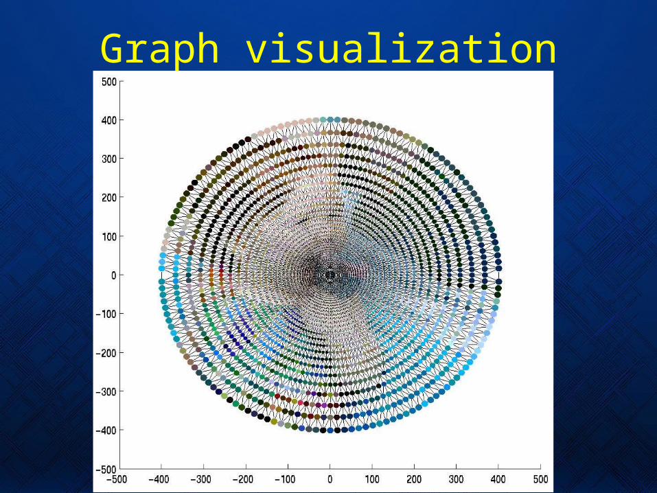
Graph visualization

Mesh visualization

Current IP algorithms

• Edge detection with 1st derivative

• Segmentation by gray level thresholding

• Mesh partitioning toolbox (Gilbert & Teng)

Edge detection

Intensity segmentation

Graph partitioning toolbox

• Failed to produce interesting segmentations for a retinal graph

• Algorithms work to produce good load balancing, and therefore will cut the retinal disk in half through the center of the fovea, regardless of the image (although the angle of the cut depends on the image)

• Algorithms may still prove useful for image guided graphs (i.e. graphs determined by image content)

Future directions:

• Coarsening/pyramid algorithms

• More serious segmentation

• Image guided graphs

• Graph matching (i.e. object recognition)

• Hardware implementation

• Fourier domain? FEM? Space/time graphs?