Seismic Noise by Wind Farms: A Case Study from the VIRGO

Gravitational Wave Observatory, Italy.

Gilberto Saccorotti1∗, Davide Piccinini1, Lena Cauchie1,2, and Irene Fiori3

1 (*corresponding author)Istituto Nazionale di Geofisica e Vulcanologia, Sezione di PisaVia U. della Faggiola, 32 - 56126 PISA (I)Tel +39 050 8311960saccorotti@pi.ingv.it

2 University College of Dublin, School of Geological Sciences - Dublin(Ireland)lena.cauchie@gmail.com

3 European Gravitational Observatory, Cascina, Pisa (Italy)irene.fiori@ego-gw.it

1

Abstract1

We present analyses of the noise wavefield in the vicinity of VIRGO,2

the Italy-France gravitational wave observatory located close to Pisa,3

Italy, with special reference to the vibrations induced by a nearby4

wind park. The spectral contribution of the wind turbines is investi-5

gated using (i) on-site measurements, (ii) correlation of spectral am-6

plitudes with wind speed, (iii) directional properties determined via7

multichannel measurements, and (iv) attenuation of signal amplitude8

with distance. Among the different spectral peaks thus discriminated,9

the one at frequency 1.7 Hz has associated the greatest power, and10

under particular conditions it can be observed at distances as large as11

11 km from the wind park. The spatial decay of amplitudes exhibits12

a complicate pattern, that we interpret in terms of the combination13

of direct surface waves and body waves refracted at a deep (≈ 800 m)14

interface between the plio-pleistocenic marine, fluvial and lacustrine15

sediments and the Miocene carbonate basement. We develop a model16

for wave attenuation which allows determining the amplitude of the17

radiation from individual turbines, which is estimated on the order of18

300-400 µms−1/√Hz for wind speeds over the 8-14 m/s range. On19

the base of this model, we then develop a predictive relationship for20

assessing the possible impact of future, project wind farms.21

1 Introduction22

Several detectors are nowadays operative to reveal the tiny space-time ripples23

which, according to Einstein’s theory of general relativity, are expected in as-24

sociation with astrophysical processes, like supernova explosions, coalescence25

of binary systems, spinning neutron stars.26

2

A class of these gravitational waves detectors (Saulson, 1994) works on27

the principle of the Michelson interferometer;28

detectors of this kind are GEO-600 in Germany, LIGO in USA, TAMA in29

Japan, and VIRGO in Italy (see The Virgo collaboration, Virgo Final Design30

1997 VIR-TRE-DIR-1000-13 available at https//pub3.ego-gw.it/itf/tds).31

Established under an Italy-France cooperative effort (EGO; European Grav-32

itational Observatory), VIRGO is located south of Pisa, about 15 km on-33

shore the central-northern Thyrrenian Coast (Fig. 1). The VIRGO laser34

interferometer consists of two 3-km-long orthogonal arms oriented N20◦E35

and N70◦W departing from a central building (CB). The end mirrors of the36

interferometer are located at the extremities of the two arms, hereinafter37

referred to as North- and West-End (NE and WE, respectively). Multiple38

reflections between these mirrors extend the effective optical length of each39

arm up to 120 kilometers, thus allowing for sensitivity to spatial strains40

on the order of ≈ 10−22 over the 10 Hz–10000 Hz frequency range. In41

order to achieve such extreme sensitivities, the interferometer exploits the42

most advanced techniques in the field of high power ultrastable lasers, high43

reflectivity mirrors, and seismic isolation systems (Acernese et al., 2010a).44

Nonetheless, intense low frequency ground vibrations might overcome the iso-45

lation system and deteriorate the detector performances. A major concern46

is that low frequency (1 Hz–10 Hz) periodic disturbances might match and47

excite the low frequency modes of the isolation systems, seriously compro-48

mising its functionality. Another concern for VIRGO is the noise associated49

to the tiny fractions of light which exits the interferometer main beam path50

and are then scattered back by external, seismically excited surfaces (Vinet51

et al., 1996; Acernese et al., 2010b).52

By mid 2008, a wind park composed by four, 2MW turbines was installed at53

3

some 6 km East of VIRGO’s NE (Fig. 1). After then, plans were submitted54

to local authorities for (i) adding three additional turbines to the existing55

wind park, and (ii) installing a new, 7-turbine wind park at a site located56

about 5 km west of VIRGO’s WE. As a consequence, EGO asked to the57

italian Istituto Nazionale di Geofisica e Vulcanologia (INGV hereinafter) to58

conduct a noise study aiming at (i) verifying properties and intensity of the59

vibrations produced by the present aerogenerators, with the ultimate goal of60

(ii) assessing the possible impact of the project wind parks.61

Wind turbines are large and vibrating cylindrical towers strongly coupled62

to the ground through massive concrete foundation, with rotating turbine63

blades generating low-frequency acoustic signals.64

Vibrations depict a complex spectrum, which includes both time-varying65

frequency peaks directly related to the blade-passing frequency, and station-66

ary peaks associated with the pendulum modes of the heavy rotor head and67

tower, and to flexural modes of the tower.68

These disturbances propagate via complex paths including directly through69

the ground or principally through the air and then coupling locally into the70

ground. Though weak, such vibrations may be relevant once compared to the71

local levels of seismic noise. Schofield (2001) found that the intense low fre-72

quency seismic disturbances from the Stateline Wind Project (Washington-73

Oregon, USA) were well above the local seismic background till distances of74

≈ 18 km from the turbines. Similar distance ranges were found by Styles75

et al. (2005), who analysed the possible influence of a project wind park at76

Eskdalemuir (Scotland), in the vicinity of the UK Seismic Array. Fiori et77

al. (2009) studied the seismic noise generated by a wind park in proximity78

of the GEO-600 interferometric antenna (Germany), and observed the signal79

from the turbines till distances of about 2000 m.80

4

In this work we present the results from seismic noise analysis in the81

vicinity of VIRGO, with special reference to the action of the wind park.82

The paper is structured into four parts. In the first part (Sections 2-3), we83

describe the geological setting of the study area and describe the data acqui-84

sition procedures. We then describe (Section 4) the spectral characteristics85

of the noise wavefield, and their relationships with human activities and the86

wind field. In the third part (sections 5 and 6), we use small- and large-87

aperture array deployments to investigate the directional properties of the88

noise wavefield and its amplitude decay with distance from the windfarm.89

In the last part (Section 7) we propose an attenuation model involving the90

combination of direct cylindrical waves propagating at the surface, and body91

waves refracted at a deep ( 800 m) lithological interface. This attenuation92

law is eventually used for establishing a predictive relationship for assess-93

ing the range of seismic amplitudes which are expected in association with94

narrow-band, shallow sources of noise.95

2 The Study Area96

EGO-VIRGO is located in the southernmost portion of the Lower Arno river,97

a Neogenic-Quaternary back-arc basin, which formed in the Middle-Miocene,98

during the Northern Thyrrenian Basin extensional phases (Fanucci et al.,99

1987; Patacca et al., 1990). This tectonic depression is bounded by the100

Monti Pisani to the north and by other smooth relief to the south (Monti101

Livornesi). The tectonic and climatic pulses during the Miocene allowed102

marine and continental deposits to overlay the Mesozoic bedrock and the103

metamorphic Tuscan Unit, previously collapsed along a set of NW striking104

normal faults (Cantini et al., 2001). As a consequence, the top of the car-105

5

bonatic bedrock deepens from depths of ≈ 700 m to depths of ≈ 2500 m as106

one moves from the eastern to the western sector of the plain (Mariani and107

Prato, 1988; Della Rocca et al., 1988). The shallow geology (up to depths108

of ≈ 60 m) is well documented by a large number of boreholes and surveys,109

which overall confirm the stratigraphic settings previously described by sev-110

eral authors (e.g., Mazzanti and Rau, 1994; Stefanelli et al., 2008). According111

to these studies, the deposition due to the glacial activity and the eustatic112

changes during Pleistocene fills up the basin with four main layers:113

i) conglomerates (Conglomerates of the Arno River and Serchio from114

Bientina) attributed to the Wurm II inter-glacial period (60 ky - 40 ky before115

present);116

ii) deep mud and fluvio-lacustrine deposits; iii) sands; iv) shallow mud117

and fluvio–lacustrine clays (Grassi and Cortecci, 2006).118

3 Data Acquisition and Processing119

Our seismic survey had the main goal of discriminating which components120

of the noise wavefield are likely due to the action of the wind generators, in121

turn determining how these signals propagate and attenuate.122

To attain these objectives, we deployed the instruments according to dif-123

ferent, time-varying configurations, designed in order to provide the best124

resolution for both directional and attenuation measurements over a wide125

frequency band and distance range. In total we used 14 seismic stations,126

three of which were kept fixed at the same location throughout the duration127

of the survey (sites 1078, 7148 and 931E in Fig. 1), while other three were128

used for short-duration measurements of site effects via H/V spectral ratios129

(not described in this paper).130

6

Our instruments consisted of nine RT130- and five 72A-type recorders131

from REFTEK, each synchronised to the GPS time signal. All mobile sta-132

tions used Lennartz LE3D-5s, three-component velocimeters exhibiting a flat133

velocity response over the 0.2-40 Hz frequency band, while two of the three134

reference sites (1078 and 7148) were equipped with Guralp CMG40, three-135

component broad-band seismometers with flat velocity response over the136

0.025-50 Hz frequency band. For all these instruments sampling rate was137

set at 125 samples/second/channel. Complementing these data are record-138

ings from two two FBA ES-T EpiSensor accelerometers and a further CMG40139

velocimeter located at VIRGO’s vertexes and central building, respectively.140

These latter instruments are part of VIRGO’s internal monitoring network,141

and are acquired at a rate of 1 KHz and successively down-sampled at 50142

samples/second/channel.143

Data acquisition started on the 26th of October and terminated on the144

17th of November, 2009.145

Before the data collection, we performed accurate huddle tests between all146

the possible combinations of recorder/sensor pairs using either noise samples147

or teleseismic signals to verify the sameness of the amplitude response of the148

different instruments over the whole frequency band of sensitivity. All the149

spectra presented throughout the following are either velocity or displacement150

amplitude spectral densities, derived from the square root of Power Spectral151

Density (PSD) estimates, calculated via Welch’s (1967) method. Wind data152

are from an anemometer located atop VIRGO’s control building, recording153

wind speed and direction at a rate of 1 datum every 10 s.154

7

4 Seismic Noise in proximity of the Wind155

Park156

4.1 Spectral Properties157

Seismic noise in proximity of the wind park exhibits a typical weekly and daily158

pattern (the 8-hr workday, for example), as depicted by the spectrogram of159

Figure 2.160

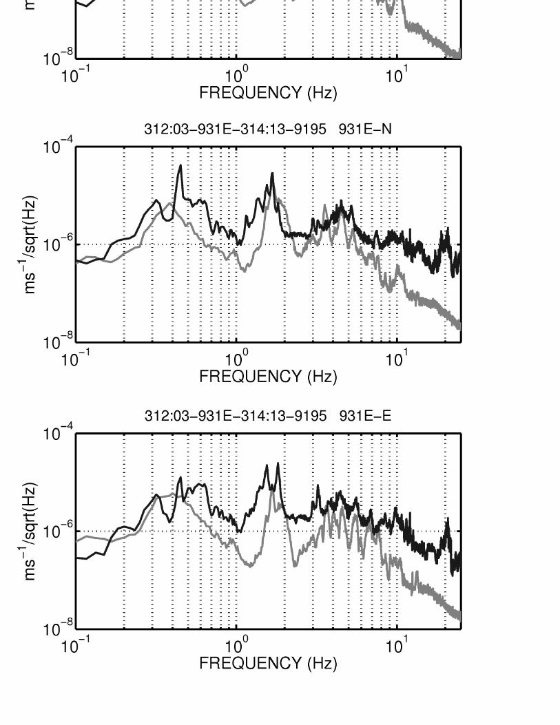
Spectra of human noise span the 1 Hz-20 Hz frequency band, as shown in161

Figure 3, where we compare spectra taken during a day and night intervals162

in absence of wind. In general, spectra taken at day time are an amplified163

version of those collected during the night, indicating that no monochromatic164

signals are generated by human activities.165

On the other side, the nightly spectra depict several narrow spectral peaks166

which origin is not likely related to anthropic noise (e.g., the peak at fre-167

quency ≈ 1.7 Hz on the NS component, and narrow peaks at frequencies ≈168

3 Hz, 4 Hz, 5.5 Hz, 7 Hz on the EW component). As it is shown in the rest169

of the paper, the peak at frequency ≈ 1.7 Hz of the NS component is the one170

which assumes the greatest relevance to the purpose of this study.171

4.2 Noise amplitude and wind speed172

Rows of the spectrogram in Figure 2 are time series of the narrow-band noise173

amplitude, that we cross-correlate against the contemporaneous time series174

of wind speed in order to verify whether particular spectral lines are coupled175

to the action of the wind. The frequency-dependent maxima of the cross-176

correlation function and associated lag times are shown in Figures 4a and177

4b for the NS component of motion. Noise exhibits a good correlation with178

8

wind speed at several discrete frequencies, centered at around 0.45, 1.7, 3.5,179

4.5 Hz.180

An example of such correlation is shown in Figure 4c where the time181

series of noise amplitude at frequency 1.7 Hz is compared with the chrono-182

gram of wind speed. At frequencies above 1 Hz, the correlation peaks of183

Figure 4a occur at zero lag (Fig. 4b); in other words, noise amplitude grows184

contemporaneously to the increase of wind speed.185

On the contrary, noise amplitude at frequency 0.45 Hz is delayed by sev-186

eral hundred minutes with respect to the wind intensity, suggesting that187

marine microseism is the most likely origin for the seismic noise at that par-188

ticular frequency.189

Correlation of seismic noise amplitude with wind speed is well documented by190

numerous previous studies (e.g., Withers et al., 1996, and references therein).191

All these works indicate however that an increase in wind speed affects seis-192

mic noise over a wide frequency band (e.g., 1 Hz-50 Hz). Our narrow-band193

correlations are therefore suggestive of an harmonic source which is itself194

excited by the action of the wind.195

4.3 Noise from an individual turbine196

Figure 5 illustrates the spectrogram for the vertical component of ground197

velocity recorded in close proximity of an aerogenerator, and encompassing198

a switch-on of the turbine. While the turbine is stopped, we recognise a199

few transients overimposed to a continuous radiation at frequency 0.45 Hz.200

We attribute this energy to the eigen-oscillation of the tower, which is occa-201

sionally excited by adjustments of the nacelle orientation. The switch-on of202

the turbine is well recognised at about 3000 s into the recording, and it is203

marked by (i) a few steady spectral lines, the most important of which are204

9

at frequencies of 0.45 Hz and 1.7 Hz, and (ii) time-varying peaks (gliding205

spectral lines), at frequencies of about 0.3 Hz, 0.6 Hz, 0.9 Hz,... up to 20 Hz206

and above. The time stationarity of the former peaks indicates that these207

are likely due to the different modes of oscillation of the tower. Conversely,208

the gliding spectral lines are attributed to the rotation of the blades which209

complete period of revolution varies within the 3-10 s range as a function of210

wind speed and nacelle orientation. Figure 6 compares spectra from beneath211

the turbine (taken at low wind speeds) with not-contemporaneous spectra212

observed at the reference site 931E during a 1-hour-long period of stong213

wind. The two sets of spectra are markedly different, and the only common214

peak is found at the Z and NS components of motion, at frequency 1.7 Hz.215

This suggests that either the other peaks that we found to correlate clearly216

with wind speed (e.g., 3.5, 4.5 Hz...) are not related to the action of the217

wind park, or that path effects, and the combination of waves radiated from218

individual turbines, modify severely the spectral composition of the seismic219

noise as it propagates away from the wind park.220

As a consequence, beneath-turbine measurements cannot be taken as rep-221

resentative of the overall wind park noise as observed in the far field. The222

next two sections are thus dedicated to finding indirect evidences for deter-223

mining the noise spectral components which are actually due to the action224

of the wind park.225

5 Directional Properties and Wavetypes226

In this section we use a dense, 2-D array deployment installed about 480 m227

from the closest turbine to investigate the composition of the noise wave-228

field around the wind park. Under the plane-wave approximation, we use229

10

inter-station delay times measured via cross-correlation to derive the two230

component of the horizontal slowness vector and hence apparent velocity231

and backazimuth for waves impinging at the array (Del Pezzo and Giudi-232

cepietro, 2002). Multichannel data streams are first passed through a bank233

of 0.2-Hz-wide band-pass filters spanning the 0.1-5.1 Hz frequency band;234

for each frequency band, inter-station cross correlations are calculated using235

non-overlapping, 600-s-long windows of signal, thus allowing for a time- and236

frequency-dependent estimates of the kinematic properties of the noise wave-237

field. We decided to use such long time windows since we noted correlation238

estimates to become stable for time windows longer than ≈ 500 s.239

The results, shown in Figure 7, clearly indicate that most of the energy240

at frequency above 1 Hz propagates from directions which are compatible241

with the wind park (backazimuths between 90◦ and 110◦). Conversely, waves242

at frequencies below 1 Hz mostly come from the coast (i.e., backazimuths243

pointing to West), confirming that marine microseism is the most powerful244

source over this particular frequency range.245

Our measurements also indicate a marked dispersion, indicating a domi-246

nance of surface waves. Phase velocities range from 1000-2000 m/s below 1247

Hz, to 100-200 m/s at frequencies above 2 Hz. These values are consistent248

with those listed by Castagna et al. (1985) for shear waves propagating in249

saturated, unconsolidated sediments. At frequency 1.7 Hz, particle motions250

at the array site are mostly horizontal, and oriented N-S (i.e., perpendicu-251

larly to the direction of propagation), thus suggesting a dominance of Love252

waves.253

11

6 Attenuation with distance254

Figure 8 illustrates the spatial decrease of spectral amplitudes as a function of255

distance from the wind park. Measurements are taken during a windy night256

(wind speed ≈ 50 km/h), for which we do expect low intensity of human257

sources and high radiation from the wind turbines.258

Several out of the frequency peaks which correlate well with wind speed259

(e.g., 1.7, 3.5, 4.5 Hz on the NS component) attenuate as one goes farther260

from the wind park, thus reinforcing the hypothesis that these peaks are due261

to the action of the turbines. In particular, the peak at frequency 1.7 Hz is262

clearly observed also at VIRGO’s WE, about 11 km from the energy plant.263

For this particular frequency, the decay of spectral amplitude with in-264

creasing distance from the source exhibits a complicate pattern (Fig. 8b).265

In particular, we observe a marked change in the amplitude decay rate for266

source-to-receiver distances on the order of 2500-3000 m.267

A simplified propagation model explaining the two different attenuation268

rates involves the combination of direct surface waves, and body waves prop-269

agating along deeper paths characterised by higher velocities and quality270

factors.271

272

In this model, if we assume an isotropic source located at the free surface,273

the amplitude of the surface waves AD(f, r) scales with distance r according274

to a general attenuation law for cylindrical waves (e.g., Del Pezzo et al.,275

1989):276

AD(f, r) =A0√re−

πfr

Q0v0 (1)

where A0 is the seismic amplitude at the source, f is the frequency, and277

12

(Q0, v0) are the quality factor and surface-wave velocity of the shallowest278

layer,respectively,.279

As for the body waves, we simplify their propagation in terms of head waves280

refracted at a deep (≈ 800 m) interface between the shallow plio-pleistocenic281

sediments and the miocene carbonates (Fig. 9). The down- and up-going282

ray segments of these waves traverse an 800-m-thick layer of average Quality283

Factor and shear-wave velocity (Q1, v1), respectively, and are continuosly284

refracted at the interface with an half-space of quality factor and velocity285

(Q2, v2). Neglecting the short propagation paths throughout the shallowest286

layer, the attenuation with distance of these body waves is thus described by287

the relationship:288

AR(f, r) = A0(2r1 + r2)−ne

−2πr1f

Q1v1−

πr2f

Q2v2 (2)

where n is the geometrical spreading coefficient which, for body waves, is289

expected to take unit value.290

Thus, for an observer recording the signal from N turbines which vibrate291

with the same amplitude A0 and are located at distances ri, i = 1 . . . N , the292

amplitude is given by the sum of eqs. (1) and (2):293

AT (f) = A0

N∑

i=1

(AD(f, ri) + AR(f, ri)) (3)

remembering however that the AR term (eq. 2) is not defined for hori-294

zontal distances r shorter than the critical distance.295

Equation 3 is based on the critical assumptions that (i) each turbine ra-296

diates a signal of the same amplitude; (ii) these signals propagate in phase,297

thus constructively interfering throughout their paths, and (iii) the energy is298

equally parted into surface- and body-wave raypaths.299

13

300

The free parameters in equation (3) are the velocities and quality fac-301

tors vi, Qi (i = 0, . . . 2) of the two layers and the halfspace, the geometrical302

spreading coefficient n of the body head waves, and the amplitude A0 of the303

radiation from each individual turbine. The depth to the top of the carbon-304

ate basement h is rather well constrained by well-log data, and as specified305

above it is assumed to take the value of 800 m.306

For fitting eq.(3) to data, we first consider a sample set of amplitude vs. dis-307

tance measurements obtained over 1-hour-long recording at 14, 3-component308

stations. For these signals, we average the amplitude spectral densities over309

a 0.1 Hz-wide frequency band encompassing the reference frequency of 1.7310

Hz, and eventually obtain three-component amplitudes from the quadrature311

sum of spectra derived at the individual components of ground motion.312

The fit is conducted using an exhaustive grid search in which all the free313

parameters in eq.(3) are allowed to vary over appropriate ranges. For A0 and314

n we used 11 values spanning the [10–1000] µms−1/√Hz and [0.5–1] ranges,315

respectively. The three Qi × vi (i = 0 . . . 2) products were instead allowed316

to vary over an 11 × 11 × 11 grid spanning the [3000,5000], [10000,80000]317

and [100000,200000] m/s intervals, respectively. These ranges encompasses318

S-wave velocity and quality factor values which are expected in association319

with the shallow geology of the site (e.g., Campbell, 2009; Castagna, 1985).320

For each combination of these parameters, we then calculate the L1 misfit321

function:322

L1(m) =

Nobs∑

i=1

|Aobs(ri)− Apre(ri)| (4)

wherem is a model vector containing the parameters (A0, n,Q0V0, Q1V 1, Q2V2),323

and Aobs, Apre are the observed amplitudes and those predicted in the sense324

14

of eq.(3). From this procedure, we noted that the misfit function (eq. 4)325

is mostly sensitive to the source amplitude and body-wave spreading coef-326

ficient. Therefore, we assigned to seismic velocities and quality factors the327

values reported in Figure 9, and inverted amplitude observations only for the328

spreading coefficient of body waves and the amplitude at the source.329

The inversion was separately applied to amplitude data taken from twenty,330

1-hour-long interval of noise recorded by different network geometries, at dis-331

tances from the barycenter of the wind park ranging from 1200 m to ≈ 11000332

m. For each set of measurements, we only considered stations for which the333

peak at 1.7 Hz was clearly visible. Best–fitting values of A0 and n were334

sought over a 21 × 21 regular grid spanning the same intervals mentioned335

above.336

337

Figure 10 shows the L1 error function from a sample data set, and the338

comparison between the observed amplitudes and those predicted on the339

basis of the minimum-norm model.340

The sample error function of Figure 10a indicates a clear correlation be-341

tween A0 and n. Nonetheless, results from the whole set of inversions depict342

narrow distributions, thus supporting the overall robustness of the estimates.343

In fact, mean values and ± 1σ uncertainties for the A0/Arif ratio (where Arif344

is the amplitude at reference site 931E) and the spreading coefficient n are345

29.9 ± 1.9 and 0.70 ± 0.04, respectively.346

347

The geometrical spreading coefficient of head waves is sensitively smaller348

than the unit value which is expected for body waves. This occurrence is349

likely due to the fact that our simplified model assumes that the source350

radiates isotropically, in turn neglecting the additional conversion to surface351

15

waves as body waves impinge at the earth’s surface.352

7 Predictive Relationship353

The points discussed above allow establishing a predictive relationship for354

assessing the effects of future wind plants with custom turbine configuration.355

As a first step, we use the results from the inversion of amplitude data to356

convert the seismic amplitude observed at the reference site to the radiation357

amplitude at unit distance from a single turbine.358

In order to relate these amplitudes to the wind speed, we consider that the359

energy in a volume of air goes as the square of its velocity, and that the360

volume that pass by the turbine per unit time increases linearly with wind361

velocity.362

Thus, the available power P at an individual turbine goes as the cube of363

the wind velocity W : P ∝ W 3.364

By further assuming that the power in the seismic signal is proportional to365

the wind power available to the turbine, it turns out that the signal amplitude366

goes as the wind velocity to the 3/2 power (Schofield, 2001; Fiori et al., 2009).367

We thus plot the single-turbine amplitudes against the wind speed for the368

entire observation period, and fit these data with a power law in the form:369

As = c+ a ·W 3

2 (5)

where As is the amplitude spectral density of the ground velocity (in370

ms−1/√Hz) at unit distance from a single turbine, and W is the wind speed371

in m/s (Fig. 11). The best-fitting parameters are a=2.13×10−7 Hz−0.5 and372

c = 1.40 × 10−6 ms−1Hz−0.5. The fit is not very well constrained, likely373

due to a combination of several causes, such as: (i) contamination of the374

16

seismic signal by additional noise sources, and (ii) difference of the wind field375

between VIRGO’s anenometer and the wind park.376

Keeping these limitation in mind, one can substitute the A0 of eq. (3) with377

the right-hand side of eq. (5), thus deriving the expected spatial distribution378

of ground vibration amplitudes as a function of wind speed, for any custom379

configuration of wind turbines. Once a robust statistics of wind speed will be380

available, these data will eventually allow to derive ’shake maps’ describing381

the probability of exceeding given ground motion amplitudes throughouit382

the study area.In this application, moreever, it must be considered that the383

wind speed measured at VIRGO’s anenometer (placed at ≈ 10 m height) is384

expected to be sensitively smaller than that at the blades’ elevation (60-100385

m).386

8 Discussion and Conclusion387

In this paper we analysed the seismic noise wavefield in the vicinity of the388

VIRGO gravitational wave observatory (Cascina, Pisa - Italy), with special389

reference to the action of a nearby wind park composed by four, 2 MW390

turbines. Using stations deployed at distances ranging between ≈ 1200 m391

and ≈ 11,000 m from the barycenter of the wind park, we obtained record-392

ings of the noise wavefield over a wide range of site condition and epicentral393

ranges. We noted that path effects modify significantly the source spectrum,394

implying that beneath-turbine measurements are not fully indicative of the395

effective contribution of the wind park to the far–field ground vibration spec-396

tra. Therefore, the spectral components of the noise wavefield likely due to397

the action of the wind park had to be discriminated on the basis of indirect398

evidences, including: (i) Correlation of narrow-band noise amplitude with399

17

wind speed; (ii) Directional properties, and (iii) Attenuation with increasing400

distance from the wind park.401

Basing on these results, we individuated several frequency bands likely due402

to the action of the wind park. Among these, the most energetic is that at403

frequency 1.7 Hz which, under particular conditions (i.e., low cultural noise404

and strong wind) can be clearly observed at epicentral distances as large as405

11 km.406

At this particular frequency, waves depict a complicate pattern of attenua-407

tion with distance, characterised by a marked decrease in the decay rate for408

ranges larger than 2500–3000 m.409

We interpreted this pattern in terms of a simplified propagation model in-410

volving the combination of direct, cylindrical waves and body head waves411

continuosly refracted at a deep (≈ 800 m) interface separating the shallow412

marine-lacustrine sediments from the carbonate basement. This model is413

based on several simplifying assumptions, including: (i) Seismic energy is414

equally parted into surface and head body waves, and no other wave types415

and/or wave conversions are allowed, and (ii) Site effects are negligible.416

By further assuming that (i) Each turbine radiates the same amount417

of energy; (ii) Signals from individual turbines sum constructively, (iii) the418

velocity structure of the propagation medium is laterally-homogeneous, and419

(iv) Local amplification effects are negligible, we thus defined a model relating420

the seismic amplitude recorded at a given distance to the radiation of each421

individual turbine.422

Assumption (ii) above is likely to provide an over-estimation of the radi-423

ation amplitude from individual turbines. A more realistic estimates should424

consider that the turbines are not all in phase and neither are they operating425

at exactly the same frequency, because of the slight possible variations in426

18

rotation speed and wind conditions across the farm. These are quasi-random427

sources and therefore add in quadrature, and not linearly as previously as-428

sumed. Therefore 100 turbines are 10 times as noisy as 1, not 100 times.429

Thus, since we’re dealing with a park composed by 4 turbines, the above430

consideration would imply scaling the estimated single-turbine amplitudes431

by about a factor 2, which is probably not so relevant once compared to the432

assumptions reported at points (iii) and (iv) above (i.e., site and path effects).433

434

Separately, we also found a relationship between wind speed and noise435

amplitude, which is reasonably well-fitted by a power law. Therefore, these436

two pieces of information allow us to build a predictive relationship linking437

wind speed with expected noise amplitude for any custom configuration of438

turbines. This latter argument will permit, given a robust statistics of wind439

speed, to assess the probabilities of exceeding an arbitrary noise amplitude440

threshold at any site of interest within the study area, as a consequence of441

present or project wind parks.442

443

9 Data and Resources444

All data used for this study are property of the EGO Consortium and cannot445

be released to the public.446

10 Acknowledgements447

Thoughtful revisions from Martin C. Chapman, Salvatore de Lorenzo and448

an anonymous reviewer greatly contributed to improving the quality of the449

19

manuscript. The research was fully supported by the EGO Consortium.450

Thomas Braun, Riccardo Azzara, Nicola Piana Agostinetti, Chiara Mon-451

tagna and Luciano Zuccarello participated to the field survey. Federico Pao-452

letti provided superb logistic assistance during the data aquisition. Finally,453

we are grateful to Jacques Colas, whose constructive criticisms greatly stim-454

ulated the conduction of the research.455

11 References456

Acernese, F., et al. (2010a) Measurements of Superattenuator seismic isola-457

tion by Virgo interferometer. Astrop. Phys., 33 , 182-189.458

459

Acernese, F., et al. (2010b) Noise from scattered light in Virgo’s second460

science run data, Class. Quantum Grav. , 27.461

462

Campbell , K.W., (2009). Estimates of Shear-Wave Q and k0 for Uncon-463

solidated and Semiconsolidated Sediments in Eastern North America. Bull.464

Seism. Soc. Amer., 99, 23652392, doi: 10.1785/0120080116.465

466

Cantini P., Testa G., Zanchetta G., Cavallini R. (2001) - The Plio-467

Pleistocene evolution of extensional tectonics in northern Tuscany, as con-468

strained by new gravimetric data from the Montecarlo basin (lower Arno469

valley, Italy). Tectonophysics, 330, 25-43.470

471

Castagna, J. P., M. L. Batzle and R. L. Eastwood (1985). Relationships472

between compressional-wave and shear-wave velocities in clastic silicate rocks473

. Geophysics, 50, 571-581.474

20

475

Del Pezzo, E., G. Lombardo and S. Spampinato, (1989). Attenuation of476

Volcanic Tremor at Mt. Etna, Sicily. Bull. Seism. Soc. Amer., 79, 1989-477

1994.478

479

Del Pezzo, E. and F. Giudicepietro, (2002) Plane wave fitting method480

for a plane, small aperture, short period seismic array: a MATHCAD 2000481

professional program. Computer and Geosciences , 28, 59-64.482

483

Della Rocca B., Mazzanti R. e Pranzini E., (1988) - Studio geomorfologico484

della Pianura di Pisa. Geogr, Fis. Dinam. Quat., 10 (1987), 56-84.485

486

Fanucci F., Firpo M., Ramella A. (1987) - Genesi ed evoluzione di piane487

costiere del Mediterraneo: esempi di piccole piane della Liguria. Geogr. Fis.488

Dinam. Quat., 10, 193-203489

490

Fiori,I., L. Giordano, S. Hild, G. Losurdo, E.Marchetti, G. Mayer, and491

F.Paoletti (2009). A study of the seismic disturbance produced by the wind492

park near the gravitational wave detector GEO-600. Proc. 3rd Int. Meeting493

on Wind Turbine Noise. Aalborg (Denmark), 1719 June 2009494

495

Grassi S., Cortecci G., (2005) - Hydrogeology and geochemistry of the496

multilayered confined aquifer of the Pisa plain (Tuscany-central Italy). Appl.497

Geochem., 20, 41-54498

499

Mariani M., Prato R. (1988) - I bacini neogenici costieri del margine tir-500

renico: approccio sismicostratigrafico. Mem. Soc. Geol. It., 41, 519-531501

21

502

Mazzanti R. , Rau A (1994) - La Geologia. In: Mazzanti R. (ed.) - La503

pianura di Pisa e i rilievi contermini. La natura e la storia. Mem. Soc. Geol.504

It., 50, 31-87505

506

Saulson P.R (1994) Interferometric gravitational wave detectors, World507

Scientific,316 ppgg.508

509

Patacca E., Sartori R., Scandone P (1990) - Tyrrhenian basin and Apen-510

ninic arcs: kinematic relations since Late Tortonian times.Mem. Soc. Geol.511

Ital., 45, 425-451512

513

Schofield R., (2001), Seismic Measurements at the Stateline Wind Project,514

LIGO T020104-00-Z.515

516

Stefanelli P., Carmisciano C., Caratori Tontini F., Cocchi L., Beverini517

N., Fidecaro F. and D. Embriaco (2008) Microgravity vertical gradient mea-518

surement in the site of VIRGO interferometric antenna (Pisa plain, Italy).519

Annals of Geoph., 51, 877-886520

521

Styles, P., (2005). A detailed study of the propagation and modelling522

of the effects of low frequency seismic vibration and infrasound from wind523

turbines. Proc. 1st Int. Meeting on Wind Turbine Noise, Berlin, Oct. 2005524

525

Vinet, J.Y. et al. (1996) Scattered light noise in gravitational wave inter-526

ferometric detectors: Coherent effects, Phys. Rev. D, 54, 1276-1286527

528

22

Welch, P. (1967). A direct digital method of power spectrum estimation,529

IBM J. Res. Dev., 5, 141.530

531

Withers, M.M, R.C. Aster, C.J. Young and Eric P. Chael (1996). High-532

Frequency Analysis of Seismic Background Noise as a Function of Wind533

Speed and Shallow Depth . Bull. Seism. Soc. Amer., 86, 1507-1515534

535

23

12 Figure Captions536

Fig. 1 - Simplified Geological Map of Western Tuscany. The shaded region537

marks the area surrounding VIRGO and object of this study. The inset at the538

bottom-right shows the configuration of the VIRGO antenna (black lines),539

with location of the recording stations which have been kept fixed throughout540

the duration of the survey. Circles are Episensor accelerometers deployed at541

VIRGO’s towers, and triangles are stations equipped with Guralp CMG-40T542

broad-band sensors. The square is the reference station 931E, equipped with543

a Lennartz LE3D-5s seismometer; stars mark the position of the four turbines544

of the windpark.545

Fig. 2 - Spectrogram for the vertical component of ground velocity546

recorded at reference site 931E (see Fig. 1). Each spectrogram’s column547

results from the average of spectral estimates obtained over 10 consecutive,548

not-overlapping 60-s-long windows of signal.549

Unit is amplitude spectral density (ms−1/√Hz), according to the color-550

bar at the right. Labels at the top of the map indicate days of the week.551

Fig. 3 - Amplitude spectral density for the three component of ground552

velocity recorded at reference site 931E (see Fig.1) during night- and day-553

time periods (gray and black lines, respectively), both in absence of wind.554

Spectral densities are obtained using 10 consecutive, not-overlapping 600-s-555

long windows of signal. The bottom panel reports the spectral ratios between556

day- and night-time measurements.557

Fig. 4 - (a) Maxima of the Cross-Correlation function between narrow558

band noise amplitude and wind speed. (b): Time lags associated with cor-559

relation coefficients greater than 0.4. (c) Time evolution of the seismic noise560

24

amplitude at frequency 1.7 Hz (NS component of reference site 931E) and561

wind speed recorded at EGO’s premise.562

Fig. 5 - Time series (top) and corresponding spectrogram (bottom) for563

the vertical component of ground velocity observed at the base of a turbine,564

and encompassing a switch-on sequence (≈ 3100 s into the record).565

Unit is amplitude spectral density (ms−1/√Hz, according to the grayscale566

at the right.567

Fig. 6 - Comparison of spectral amplitudes observed beneath a turbine568

and at reference site 931E (black and gray lines, respectively). The two data569

set are not simultaneous, and correspond to wind speed of ≈ 3 m/s and ≈570

11 m/s, respectively.571

Fig. 7 - (a) Dispersion curve, derived from the frequency-dependent572

slowness estimates. Slowness data are obtained from 24 consecutive, not-573

overlapping 600-s-long time windows. The inset shows the configuration of574

the array used for slowness estimates (circles), with respect to the wind575

park (stars). (b) Wave Backazimuth (direction-of-arrival) as a function of576

frequency. The two dashed lines mark the angular interval encompassing the577

wind park.578

Fig. 8 - (a) Spatial decay of the amplitude of ground velocity (N com-579

ponent) for increasing distance from the barycenter of the windpark. The580

image map is the logarithm of the amplitude spectral density (ms−1/√

(Hz))581

, according to the colorbar at the top. The peak at frequency 1.7 Hz is clearly582

observed at VIRGO’s west end, ≈ 11 km from the wind park. (b) Spatial583

decay of the amplitude at the frequency 1.7 Hz. The decay rate changes584

abruptly for distances on the order 2500–3000 m, suggesting the emergence585

25

of waves which propagated through deeper paths.586

Fig. 9 - Sketch of the propagation model used for interpreting amplitude587

data. Seismic waves radiated from a source at the surface propagate as both588

surface waves and body head waves refracted at a deep interface; XC is the589

critical distance. Surface waves are entirely confined within the shallowest590

layer, while body waves propagate through a layer of thickness h and at the591

interface between this layer and an halfspace represented by the carbonate592

basement. Shear-wave velocities and quality factors are listed within each593

layer.594

Fig. 10 - (a) L1-norm misfit function obtained from the regular grid-595

search over the parameters A0 and n for fitting equation 3 to three-component596

amplitude data. (b) Fit of experimental, three-component amplitudes using597

the best values of the parameters obtained from the minimum of the misfit598

function in (a)599

Fig. 11 - Relationships between vibration amplitude at a single turbine600

and wind speed. Gray tones indicate wind directions measured clockwise601

from North, according to the gray scale at the right.602

26

618 620 622 624 626 628 630 632

4828

4830

4832

4834

4836

4838

EASTING (km)

NO

RT

HIN

G (

km

) EPNE

EPWE

CMGV1078

7148

931E

43.7

12.5

0 5 100

0.2

0.4

0.6

0.8

FREQUENCY (Hz)

CO

RR

. CO

EF

F.

(a)

0 5 10

0

200

400

600

FREQUENCY (Hz)

DE

LAY

(m

in)

(b)

300 302 304 306 308 310 312 314 3160

5

10

15(c)

DATE (JDAY 2009)

Wind Speed (m/s)ms−1/sqrt(Hz) x 1E+6

0 2 4 6 8 10 12 140

0.2

0.4

0.6

0.8

1

1.2x 10

−5

Wind Speed (m/s)

Am

plitu

de (

ms−

1 /sqr

t(H

z))

F=1.7 Hz

0

50

100

150

200

250

300

350