seismic data processing with the wave …sep · seismic data processing with the wave equation the...

SEISMIC DATA PROCESSING WITH THE WAVE EQUATION

The coordinate frames used by theoreticians to describe wave propagation do not include frames in common use by geophysical prospectors to describe observations. Whereas the theoretician generally considers a single source (or shot) location at a time, the experimentalist deals simultaneously with waves which have been gener- ated separately by many shots. Our task in this section is to put the wave equation into some prospectors' coordinate frames.

11-1 DOWNWARD CONTINUATION OF GATHERS AND SECTIONS

Suboceanic prospecting is generally carried out by a ship which carries a repetitive energy source and which trails a cable that is 2 to 3 kilometers long and packed with sonic receivers. Ideally, the ship's course is a straight line which we can take to be the x axis. Ideally, all the seismic waves of interest propagate in a vertical plane through the line of the ship's course. This plane is called the plane of the seismic section. Despite the fact that it is no great problem to describe waves in

three dimensions once difference techniques have been mastered for two dimensions, we will restrict the theory to two dimensions in order to keep it compatible with the bulk of present-day surveying practice and the capability of most present-day computing machines. An impulsive wave from a point source spreading out in three dimensions will decay in amplitude in inverse proportion to the travel time. (The area of a spherical wavefront increases as t 2, so the energy per unit area decreases as t2, and so the wave amplitude is proportional to t-l.) An impulsive wave from a line source (the line would be on the ocean's surface perpendicular to the ship's course) has an amplitude decay proportional to t-1/2. Thus, the attempt to compress three-dimensional reality into a one- or two-dimensional mathematical form often begins (and almost always ends) with a t1f2 or a t scaling factor. Of far more practical importance than this scaling is the attempt to keep all the seismic rays which emanate from and return to the ship's traverse line confined to a single plane. In other words, we hope to avoid recording side echoes. Often side echoes can be reduced or eliminated by careful choice of the ship's course. But, once the data have been recorded, you have to live with what- ever side echoes are there. One way to think about these side echoes is to imagine the ship's traverse line as the axis of a cylindrical wordinate system. Instead of considering that the time delay of an echo is a measure of the depth to a reflector, one now imagines that the travel time is a measure of the radius in the cylindrical coordinate system. Interpretation is easy if the plane of the seismic section is merely somewhat tipped away from the vertical. Interpretation problems arise when the earth is so three-dimensionally complex that several wobbly planes are involved and the observed data have become a superposition of many of them. In short, where the earth gets three-dimensionally inhomogeneous you cannot get along very well with two-dimensional experimental and calculational techniques.

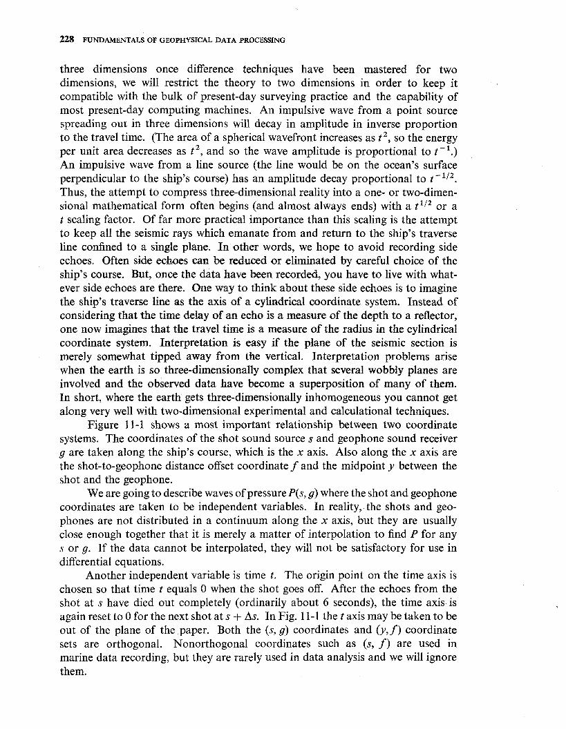
Figure 1 f -1 shows a most important relationship between two coordinate systems. The coordinates of the shot sound source s and geophone sound receiver g are taken along the ship's course, which is the x axis. Also along the x axis are the shot-to-geophone distance offset coordinate f and the midpoint y between the shot and the geophone.

We are going to describe waves of pressure P(s, g) where the shot and geophone coordinates are taken to be independent variables. In reality, the shots and geophones are not distributed in a continuum along the x axis, but they are usually close enough together that it is merely a matter of interpolation to find P for any s or g. If the data cannot be interpolated, they will not be satisfactory for use in differential equations.

Another independent variable is time t. The origin point on the time axis is chosen so that time t equals 0 when the shot goes off. After the echoes from the shot at s have died out completely (ordinarily about 6 seconds), the time axis is again reset to 0 for the next shot at s + As. In Fig. 11-1 the t axis may be taken to be out of the plane of the paper. Both the (s, g) coordinates and (y, f ) coordinate sets are orthogonal. Nonorthogonal coordinates such as (s, f ) are used in marine data recording, but they are rarely used in data analysis and we will ignore them.

. . . . . . . . . . . . . . - : - - - . g L.

profile • v A b

- * * \ . . . . . . I t . . . . receiver cable 0 . . . . . . * . . . . . . ' 0 .

I . . . . , .

FIGURE 11-1 The relationships among sound source coordinate s, geophone sound receiver coordinate g, offset coordinate f = g - s, and midpoint coordinate y = (g + s)/2. Theoreticians generally use s and g as coordinates of the wave-pressure field, but interpreters generally use f and y.

Theoreticians usually work in the (g, t) plane for a fixed s. In exploration seismology, data in the (g, t) plane are called a projile. Seismic data interpreters usually work with wave amplitude in both the (y, t) plane and the (f, t) plane. A display in the (y, t) plane is called a seismic section. A display in the (f, t) plane is called a common midpoint gather or a common reflection point gather, which, unfortunately, in industry is often called a common depth point gather. This termi- nology originated in the days when analytical methods usually modeled the earth as a stratified medium in which the reflection point, called the depth point, lay directly beneath the midpoint. It is unfortunate because of the considerable con- fusion we now have with the depth z axis. In this book we will avoid the term depth point. A data display over midpoint y at fixed offset f, that is, the (y, t ) plane, is called a seismic section and it is the only one of the orthogonal planes

which may continue for hundreds or thousands of kilometers. Projiles and gathers continue for only a few kilometers, first because of the limited length of the receiver cable, but more fundamentally because of the limited distance over which a shot can be heard.

Profiles and gathers today typically contain about 48 seismic traces. Because useful data often lie beyond the 3-kilometer receiver cable, another form of data recording is sometimes used. This is the sonobuoy. A sonobuoy is a buoy with a single sound receiver (called a hydrophone) and a radio transmitter. The buoy is cast over- board and the ship sails away, firing at about a six-second repetition rate until the buoy is out of range of either the radio or the seismic signals. Such data form a common receiver point gather and comprise about 200 to 2000 seismic traces. Sonobuoy data are conceptually one of the easiest kinds of data to be imagined as providing boundary conditions for wave-extrapolation equations. The principle of reciprocity says that we could imagine that the ship had carried the sonic receiver and that the buoy had carried the repetitive sound source. (It is not done this way because the sonic receiver is an inexpensive, lightweight, throwaway item, well suited to the buoy.) Thus, the principle of reciprocity which says P(g, s, t ) =

P(s, g, t) enables us to imagine a single shot with many hundreds of receivers, just what we need for downward continuation of the upcoming and downgoing wave fields.

This brings us to the concept of how we learn about the interior of the earth by means of downward continuing waves. As indicated in Fig. 11-2, an obvious, but important, idea is that reflectors exist in the earth at places where the onset of the downgoing waue is time coincident with an upcoming waue.

To best illustrate this idea, monochromatic waves will be used. This enables us to compute and think in (x, z) for fixed co rather than to have to work in the three- dimensional space of (x, z, t). A penalty we pay by going to a single frequency is that the idea of time coincidence of two time-dependent waveforms becomes for monochromatic waves the idea of both waves being coherent with a fixed phase shift (usually zero or 180 degrees) at points in space where reflection can occur. We will see that phase equivalence at a single frequency at a single point in space does not by itself provide time coincidence. The same must be true of other frequencies. Generally, the more frequencies are involved in phase coherency, the better will be the spatial resolution.

The reader will recall that a number of assumptions in Sec. 10-5 led us to the idea that up- and downgoing monochromatic waves can be calculated with equations like

In a forward problem, synthetic data are calculated from a model. In an inverse problem, a model is calculated from the data. To do a forward problem we

FIGURE 11-2 Illustration of the basic principle of reflector mapping. There are a near- surface source S and many surface receivers R. At a shallow depth above the reflector at the typical point PI the downgoing wave Dl occurs much earlier than the upcoming wave U l . The upgoing wave Ul represents energy which has traveled from the source to one or more places on the reflector and then back up to the point PI. At a point P,, which is at or near a reflecting interface of arbitrary shape, there will be overlap in time of the down- and upgoing waves D, and U,. The time overlap may be used in the construction of a map of reflector positions. Below the reflector at the point P3, there is, in principle, no upcoming wave. However, practical schemes for estimating the upcoming waves U at various depths in large part amount to shifting the upcoming waves seen at R to earlier and earlier times corresponding to greater and greater depths. Since the practical schemes will have no knowledge of the interface, they will predict an erroneous upcoming wave U3 at P3 , indicated by dots before the arrival of the downgoing wave. This error has no bad effect on the reflector mapping formulas which utilize time coincidence of up- and downgoing waves. These ideas are valid in situations where there are many reflectors at many depths. (From Ref. [ 5 ] , p. 468.)

first assume a shot location at, say z = 0 and x = 0. This provides a delta function initial condition for the downgoing wave. Assumption of a velocity model then allows use of an equation like, say (1 1-1-1) to continue the downgoing wave downward to arbitrary depth. At a sufficiently great depth, the upcoming wave U is taken to be 0. It is integrated upward with (1 1-1-2) where the product of the reflection coefficient c and the downgoing wave D act as a source for the upgoing wave.

Now we approach the inverse problem where we are trying to determine the reflection coefficient c(x, z), but we are given the observation of the upgoing wave U at the earth's surface (z = 0, all x). We calculate D as before. Since c(x, z ) is

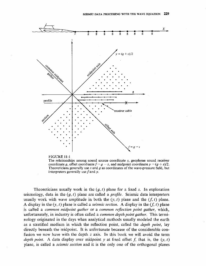
FIGURE 1 1-3 Location of a dipping bed with a single source emitting a single frequency. Top and bottom represent two possible source locations. The left-hand panel shows the real part of downgoing wave D. The dashed line represents a transition from low to high velocity as can be seen by the greater wavelength below. The center panel represents the upcoming reflected wave U, which originates at the velocity jump. On the right-hand panel is plotted the real part of the ratio O/D. The right- hand panel tells where downgoing and upcoming waves are in phase. It gives the correct dip of the bed. With only a single frequency the depth cannot be deter- minded except to within multiples of a half-wavelength. The estimated upcoming wave 0, is computed from the true upcoming wave U, observed at the surface and the velocity v of the medium; Y,/ Y is not used. (From Ref. 131, p. 417.)

unknown in (1 1-1-2) we can compute 0 , an approximation to U, by marching the equation

down from the surface z = 0 where 0 is given. Now the question is, how will 0 depart from U? Between the earth's surface

and the shallowest reflector (shallowest nonzero c) there will be no difference between (1 1-1-2) and (1 1-1 -3). In that region, both U and 0 will be waves of identical speeds, directions, rates of divergence, and all other properties. As (11-1-2) is

projected downward (opposite to the direction of propagation), the source terms in (1 1-1-2) serve to "turn off" the upcoming waves until U, unlike 0, totally vanishes beneath the deepest reflector. Now the question is whether there is practical significance to the fact that 0 does not vanish beneath reflectors. Our purpose in computing 0 is to determine the location of reflectors by the time-coincidence idea in Fig. 11-2. For this time-coincidence idea, it does not matter that the upcoming wave is not turned off beneath an interface. Figure 11-3 illustrates these concepts for a monochromatic wave. To display the earth model, the reflection coefficient c(x, z) is estimated by displaying t where

Monochromatic Down going wave model reconstruction Model

Returned wave Reconstructed return Four frequency reconstruction

FIGURE 11-4 Synthesis of waves from a reflector which is warped and offset by a fault and the reconstruction of an image of the fault. Top left is the wave traveling away from a point source. Bottom left shows the upgoing reflected wave. It vanishes below the interface. At the bottom center, we see the reconstruction from surface observations of the upcoming wave. In doing the reconstruction, one does not assume knowledge of the reflectors, since they are what we are looking for. Hence, in the reconstructed return, one has an upgoing wave below the reflector. At the top center panel we show the product of the upgoing wave with the complex conjugate of the downgoing wave. The reflector exists along some line of zero phase, but with a single frequency, one cannot tell which line represents the reflector. The top center panel was summed over four frequencies to get the lower right panel, which gives a better indication of the reflector position. More frequencies would define it more clearly. (From Ref. [5 ] , p. 479.)

234 FUNDAMENTALS OF GEOPHYSICAL DATA PROCESSING

We notice that for a monochromatic wave there will be phase coincidence of 0 and D not only at the reflector but also at half-wavelength intervals both above and below the reflector. (If we had U instead of 0 , there would be 0 below.) Now the idea is that we can repeat the whole calculation for monochromatic waves at other frequencies and sum the results. The summation will always be in phase at the reflector but of variable phase away from the reflector.

Figure 11-4 shows a calculation like that in Fig. 11-3, but more terms were included in the equations (in order to better represent waves traveling at larger angles from the vertical) and more frequencies were used (in order to illustrate construc- tive interference at the reflector). Another difference between Figs. 11-3 and 11-4 is that the reflector estimate is O/D in (1 1-1-3), but in (1 1-1-4) it is OD* (where D* is the complex conjugate of D). Both O/D and OD* have the same phase, but they have a different amplitude. The advantage of O/D is that it has the magnitude of the reflection coefficient. The disadvantage of O/D is that nodes in D, which theoretically should imply nodes in U, may cause us to have practical problems with division by small numbers. Another advantage of OD* is that if it is to be summed not only over many frequencies, but also over many shot locations, it has the desirable characteristic that it is small where illumination is poor and large where illumination is good.

Next we attack the important practical matter of how to continue sections downward. The obvious approach is to solve a separate problem in the (g, t ) plane for each shot point. Alternatively, we could use the reciprocity principle and use each receiver point as a separate problem in the (s, t) plane. For reasons we will come to recognize, there are considerable practical advantages in leaving the theory (g, s) coordinates and continuing downward directly in the interpreter's (y, f ) coordinates. A compelling practical reason is that many data are collected with a single shot and a single receiver which move together 'across the surface of the earth. For a fixed shot point there is only one receiver point, so there are clearly insuf- ficient data to initialize a downward continuation in the (g, t ) plane. Nonetheless, when all shot points are considered, it turns out that with good accuracy we can continue the constant offset section downward.

We will develop two separate equations, one for downgoing waves and one for upcoming waves. The conversion from field coordinates (s, g, e, t) to interpretation coordinates (y,f, z, t ') is accomplished with the definitions

The first two definitions (11-1-5a, 11-1-5b) are merely the transformation from shot s and geophone g coordinates to midpoint y and offset f coordinates described

earlier. Equation (1 1-1-5c) indicates that the receiver elevation e is a point on the vertical z axis. In (1 1-1-5d) we have a definition of receiver-elevation-dependent time t'. Comparing to Sec. 10-4, it is clear that the plus sign is for waves propagating in the + z direction (down) and the minus sign giving t + z/E is for waves going up. It is important to distinguish the constant velocity fi in the coordinate transform (1 1-1-5) from the spatially variable velocity G(x, z) which will be used in the wave equation. Although the coordinate transformation is based on a constant- velocity medium, the transformed wave equation can still describe waves in a variable-velocity medium.

Now we state that we are trying to describe the same disturbance in the new coordinate system as that in the old one.

Next, we compute the partial derivative of P with respect to its independent variables.

Now we need the second partial derivatives of P with respect to its independent variables. Since all the coefficients of a,, df , at, , and a, in (11-1-7) are constants, then the second derivatives can be found by squaring the operators in parentheses in (11-1-7).

We are familiar with the wave equation in the form

P,, + Pzz = c-~P,, + source (1 1-1-8)

We can imagine that the geophones used to observe P could be placed anywhere in the (x, z) space. A quantity like P,, on the surface of the earth could be measured by setting out geophones at g = x and measuring P,,. We regard the coordinates of the geophone location (x, z) = (g, e) as independent variables. Thus, we may write the wave equation as

where we have used a source term defined as a delta function at (x, z, t) = (s, 0,O). Since we do not intend to use this equation in the vicinity of sources, we can drop the delta function at the source. Now we take the operators in (11-1-7), square them and insert them into (1 1-1-9). This gives


First we will neglect Q,, in a Fresnel-like approximation. (Higher accuracy can be achieved as in Sec. 10-3 if Q,, is estimated.) specializing to homogeneous media, v = v" and using t: = -(+ 1/Zi) and t i = 1 our equation has reduced to

Equation (I 1-1-1 1) is a partial differential equation in four dimensions starting from initial conditions which are data in three dimensions. Frequently a problem of this magnitude will not be computationally feasible, so we now consider how to remove the offset dimension. Let us integrate (1 1-1-1 1) over offset. We obtain

Now if Q and Qf should vanish at the great offsets which we take to be the limits on the integrals, then the two terms farthest right vanish. Let us define a vertically stacked section by

This stacking is done without time shifting; hence, it is similar to but not precisely the same thing as the familiar common reflection-point stack. Thus, for vertically stacked sections we have

We could also have obtained (1 1-1 - 14) from (1 1-1 - 1 1) by merely asserting that for zero-offset data the offset derivatives may be neglected and that (1 1-1 - 14) applies to near-trace sections.

Of course (1 1-1 - 14) is no stranger to us. Earlier we learned how the equation P,, = .5 UP,, controls propagation of a wave field (like a common shot-point gather). This means that (1 1-1 -14) should convert hyperbolas to other hyperbolas ; but in fact, because of the Fresnel-like approximation (which is improvable) it converts parabolas to other parabolas. In other words, (1 1-1-14) does just the kind of thing which is of use in seismic migration. Further details are in succeeding sections.

11-2 WAVE EQUATION MIGRATION

The construction of a cross section of reflectivity within the earth from a seismic section is called migration. At many locations on the earth the subsurface consists of horizontally layered sedimentary rocks. At such locations the migration of seismic data can be extremely simple because waves propagate vertically to the reflectors and they will have a round-trip travel time which is in direct proportion to depth. Migration is, then, just applying the proportionality factor to the time axis.

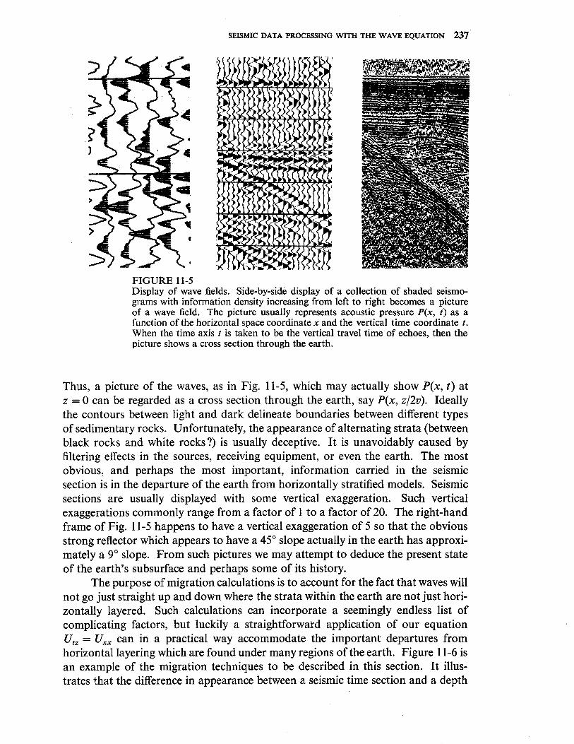
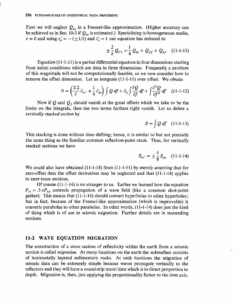
FIGURE 11-5 Display of wave fields. Side-by-side display of a collection of shaded seismograms with information density increasing from left to right becomes a picture of a wave field. The picture usually represents acoustic pressure P(x, t ) as a function of the horizontal space coordinate x and the vertical time coordinate t. When the time axis t is taken to be the vertical travel time of echoes, then the picture shows a cross section through the earth.

Thus, a picture of the waves, as in Fig. 11-5, which may actually show P(x, t ) at z = 0 can be regarded as a cross section through the earth, say P(x, 212~) . Ideally the contours between light and dark delineate boundaries between different types of sedimentary rocks. Unfortunately, the appearance of alternating strata (between black rocks and white rocks?) is usually deceptive. It is unavoidably caused by filtering effects in the sources, receiving equipment, or even the earth. The most obvious, and perhaps the most important, information carried in the seismic section is in the departure of the earth from horizontally stratified models. Seismic sections are usually displayed with some vertical exaggeration. Such vertical exaggerations commonly range from a factor of 1 to a factor of 20. The right-hand frame of Fig. 11-5 happens to have a vertical exaggeration of 5 so that the obvious strong reflector which appears to have a 45" slope actually in the earth has approxi- mately a 9" slope. From such pictures we may attempt to deduce the present state of the earth's subsurface and perhaps some of its history.

The purpose of migration calculations is to account for the fact that waves will not go just straight up and down where the strata within the earth are not just horizontally layered. Such calculations can incorporate a seemingly endless list of complicating factors, but luckily a straightforward application of our equation U,, = U,, can in a practical way accommodate the important departures from horizontal layering which are found under many regions of the earth. Figure 1 1-6 is an example of the migration techniques to be described in this section. It illustrates that the difference in appearance between a seismic time section and a depth


FIGURE 11-6 Three sinusoidal reflectors at increasing depths (left) and the calculated zero- offset reflection seismic section (right). There is no vertical exaggeration. Since each reflector has the same shape, it must have the same maximum dip (about 15") as the others. The departure of the time section from the depth section obviously increases as one looks down the frames. A rule of thumb is that significant departure begins to occur when the depth becomes comparable to the smallest radius of curvature of the reflector (buried focus). The radius about equals the depth at the shallowest reflector where strong focusing is apparent. (From Ref. [81, p. 758.)

section need not arise solely from the dip of the strata; in fact, the curvature is usually the major factor. Hence, migration can be important even in relatively flat areas.

An impulse incident on an interface gives an impulsive reflection; however, there is always some filtering effect in the source, receiver, or earth which converts the supposed impulsive waveform to a little wavelet. Ideally, the cross section through the earth should display an impulse at the interface, but the migration computation carries the wavelet from the time section into the depth section. In this way, a resolving power limitation on the time axis is converted to a resolving power limitation on the depth axis. An interesting question is that of the resolving power on the horizontal x axis. Waves propagating at an angle convert the resolving power of the wavelet to an angular axis rather than the vertical axis. Clearly, the best horizontal resolving power you could get would be from waves traveling horizontally. For 45" waves, horizontal resolving distance would be l/sin 45" times as great as the vertical resolving distance. This is illustrated in Fig. 11-7 and in other figures.

The basic operation of migration can be understood in simple terms without reference to the wave equation. Figures 11-8 and 11-9 illustrate the transforma- tions between time and depth for the two special cases where one domain or the other contains only an impulse function. Real data comprise a continuum in (x, t ) ,

FIGURE 11-7 Reflections from oscillatory interfaces illustrating lateral resolving-power limitations. On the left is a starting model of some oscillatory interfaces. Center is the construction of a zero-offset section by the method of this section extended to the 45" approximation and modified by numerical viscosity to reject energy with dips beyond about 30". The right-hand frame is the attempted reconstruction of starting model. It is no longer possible to resolve short-wavelength oscillations on the left-hand side of the interface. (From Ref. [8], p. 759.)

but Fig. 11-8 suggests a migration technique based on the linear superposition principle; namely, take every data point in the (x, t ) domain and throw it out to a circular arc in the (2, t ) domain. The migrated section is the superposition of all these arcs. A natural question one might ask is: Why bother to use the wave equation for migration when it can be done with the circular arcs? The answer to such a question depends upon a multitude of practical factors, some of which are data-dependent. One consideration favoring the wave equation approach is that velocity inhomogeneity is more easily and accurately described by wave equations than by ray tracing. Both methods are presently commercially available.

Figure 11-10 is an example which illustrates the origin of the term migration. It shows that a dipping interface which terminates at a point will appear in the time data to have the termination point migrated down-dip from its true location. In an example of this type, the departure of the depth section from the time data is really rather modest and it becomes even more slight as the dip is decreased.

This does not imply that data with slight dips need not be migrated because, as we have seen, of the dominating importance of curvature. An interesting practical example of this is shown in Fig. 11-1 1.

Field data examples of many of the synthetic data analyses are shown in the data of Fig. 1 1-1 2.

FIGURE 1 1-8 The depth response to time-domain impulses and reconstruction of the impulses. The fact that the left frame is mostly blank depicts a situation in which no echo is received when a source and receiver move together in the horizontal direction until they reach the right-hand edge of the frame where the three blips indicate that there are three echoes at successively increasing times. With these as observed data, the logical conclusion is that the reflection structure of the earth is three concentric circles with centers on the right-hand margin. The center frame shows the circles. (For economy, the right-hand edge of the frame is a plane of symmetry.) It will be noticed that the bottom of the circles is darker than the top. This is indicative of the 45" phase shift of bringing two-dimensional waves from a focus away from the focus. Waves with dips greater than about 45" have been filtered away by numerical viscosity. The loss of this energy plus the loss of the energy of waves which propagate at complex angles results in a reconstruction (right-hand frame) in which the impulses are somewhat spread out in the horizontal direction. (From Ref. [8], p. 750.)

We begin the explanation of how to migrate sections by recalling the basic result of Sec. 11-1 (and replacing t' by t).

Equation (1 1-1-13) defines a sum over offset of all the waves. Equation (1 1-1-14) shows how the sum S can be extrapolated down into the earth from the surface where it is known. We recall that the plus sign or the minus sign is chosen according to whether the extrapolation is done on the downgoing wave or the upgoing wave. Recall a source term 6(g - s, e, t) in (1 1-1-9). In midpoint-offset coordinates this source term becomes 6(f) const(y)6(~)6(t). Since the source term is a constant

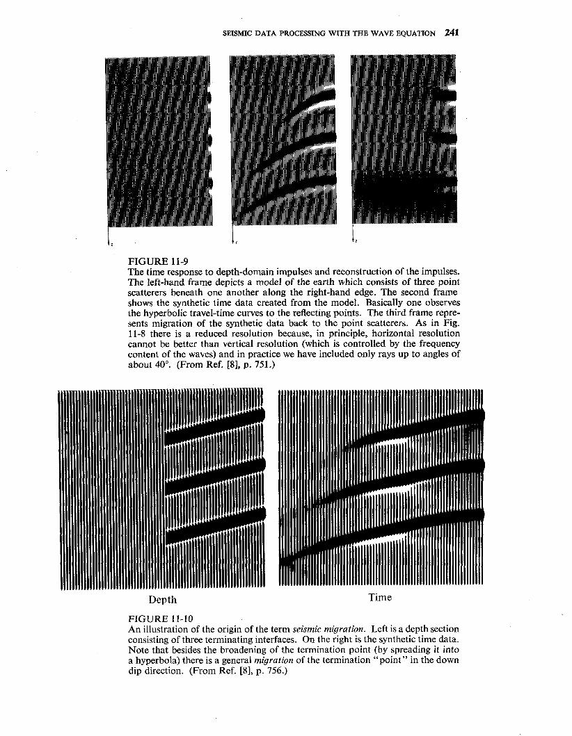
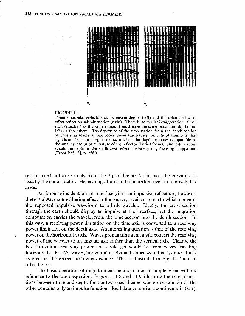
FIGURE 11-9 The time response to depth-domain impulses and reconstruction of the impulses. The left-hand frame depicts a model of the earth which consists of three point scatterers beneath one another along the right-hand edge. The second frame shows the synthetic time data created from the model. Basically one observes the hyperbolic travel-time curves to the reflecting points. The third frame represents migration of the synthetic data back to the point scatterers. As in Fig. 11-8 there is a reduced resolution because, in principle, horizontal resolution cannot be better than vertical resolution (which is controlled by the frequency content of the waves) and in practice we have included only rays up to angles of about 40". (From Ref. [8J, p. 751.)

Depth Time

FIGURE 1 1-10 An illustration of the origin of the term seismic migration. Left is a depth section consisting of three terminating interfaces. On the right is the synthetic time data. Note that besides the broadening of the termination point (by spreading it into a hyperbola) there is a general migration of the termination "point" in the down dip direction. (From Ref. [8], p. 756.)


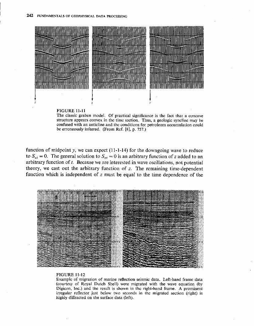
FIGURE 11-11 The classic graben model. Of practical significance is the fact that a concave structure appears convex in the time section. Thus, a geologic syncline may be confused with an anticline and the conditions for petroleum accumulation could be erroneously inferred. (From Ref. [8], p. 757.)

function of midpoint y, we can expect (1 1-1-14) for the downgoing wave to reduce to S,, = 0. The general solution to S,, = 0 is an arbitrary function of z added to an arbitrary function oft. Because we are interested in wave oscillations, not potential theory, we cast out the arbitrary function of z. The remaining time-dependent function which is independent of z must be equal to the time dependence of the

FIGURE 11-12 Example of migration of marine reflection seismic data. Left-hand frame data (courtesy of Royal Dutch Shell) were migrated with the wave equation (by Digicon, Inc.) and the result is shown in the right-hand frame. A prominent irregular reflector just below two seconds in the migrated section (right) is highly diffracted on the surface data (left).

source function; that is, a delta function of time. Since we now have an analytic function for the downgoing S at all depths, we can next turn to the numerical downward extrapolation of the upcoming S. Equation (1 1-1-14) with the minus sign enables us to do the downward extrapolation of the upcoming wave. Because the downgoing wave is a plane wave, the upcoming wave, if seen down at the reflectors, will take on the shape of the reflectors. Thus, the migrated section comprises the surface observations extrapolated downward to the proper depth.

As a practical matter, it turns out that investigators do not presently use the vertical stack defined by (1 1-1-13). They inject a time shift as a function of offset before doing the summation. The main effect of this is to make all offset traces more closely resemble the zero offset trace. The time delay of waves recorded on a zero offset section is equally divided between the downgoing path and the upgoing path. The two paths have unequal delays when the downgoing wave is a plane wave and the upcoming wave represents complicated scattering. From these con- siderations, we can now guess a result from (1 1-3-18) which is that the migration equation for a zero offset section, or an NMO stack resembles (1 1-1-14) but contains an extra factor of 2. Thus, we begin with

There may be some practical justification in allowing fi to be variable in some of the three coordinates (y, z, t); however, by keeping the velocity constant in y we can simplify our first encounter with the details of migration. Fourier transforming the y variation with eiky we reduce (1 1-2-1) to

Now we will discretize the z and t coordinates. Then the function Q in (11-2-2) may be tabulated in the (z, t) plane and the differential operator in (1 1-2-2) becomes a 2 x 2 convolution operator in this two-dimensional plane. The operator is

Defining a scale factor

the operator multiplied by Az At is

When the operator (1 1-2-5) is laid upon an arbitrary place in the Q table and the four numbers in the operator are multiplied onto the four Q numbers beneath the operator, the meaning of (11-2-2) is that the sum of these four products should vanish. If we find a place in the Q table where only three of the four numbers of Q

are actually known, then we can calculate the fourth, unknown number. In fact, Q may be given only along a few boundaries in the (z, t) plane and we may be able to fill in the rest of the plane.

Migration and its inverse may be thought of on the following grid.

On this grid r, , r,, . . . , r4 represents the observed surface seismogram and c,, c,, . . . , c4 represents the migrated section. The zeros in the bottom row represent the idea that seismograms vanish at a sufficiently late time. Notice that in filling in the table there is a lot more work (diffraction) in going from r4 to c4 than in going from r2 to c2 . This is because for fixed dip, deep events migrate farther than shallow events. Letting ky2 = 0, we have a = 0 and we are describing a stratified earth. Starting with surface data r,, r2 , r3 , and r4 and the bottom row of zeros we can use (1 1-2-5) to fill in the table (1 1-2-6) and it becomes

Inspecting the table (1 1-2-7) we see that numbers remain absdlutely constant as we move in the z direction. If we had not taken ky2 = 0 but had instead taken k; to be small, we would see the numbers in the table changing gradually in the z direction. When k: is not zero some caution must be exercised in the order in which the (z, t) plane is filled up. The number a is always positive. Obviously, if the number a happens to equal + 1, then it will be impossible to find unknown numbers in the Q table if they should lie under the multiplier 1 - a. It turns out that, regardless of what numerical (positive) value a takes, the process of recur- sively seeking numbers in Q which underlie 1 - a will be unstable as is polynomial

division by a nonminimum-phase filter. One reason is that such a process actually is polynomial division but the polynomials are two-dimensional polynomials. These complications are all the mathematical manifestations of the physical idea of causality.

From the point of view of solving hyperbolic differential equations it is most economical if you can get roughly the same number of points per wavelength (typically eight) on each coordinate axis. This means that in the development till now we have drastically over-sampled the z axis. The 15" limitation of the Fresnel approximation implies that Az could always be taken five times or more coarser than u At. The subject of optimal selection of grid spacings is somewhat involved. Suffice it to say here that some field data have been migrated satisfactorily at a Az/u At ratio as great as 100 with a corresponding reduction in cost. Anyway, for the purpose of illustrating the point we will now redraw the section table with twice as coarse a sampling on the z axis. Numbers in the two tables below indicate two different possible orderings, both causal, of the use of (11-2-5) for the migration calculation. In either case the resulting migrated section is interpolated (perhaps very crudely) off the diagonal.

t t + z-outer t-outer

The reader should check in each of the above tables that the number computed at any stage is based on three already known table entries and that the unknown being computed multiplies (1 + a) and not (1 - a). To synthesize data from a hypothetical depth section the calculation proceeds in reverse numerical order.

Study of the two optional procedures (1 1-2-7a) and (1 1-2-76) reveals that the one labeled " t-outer" has an extraordinary advantage over the one labeled " z-outer " in the much smaller computer memory requirement.

Another practical reality is the need to be able to handle depth-variable velocities. This can be achieved by taking the migrated data c,, c, , . . . , not from the diagonal in the (2, t) plane, but from another curve through the (z, t ) plane as illustrated in Fig. 11-13. A nice feature of wave-equation migration is that velocity


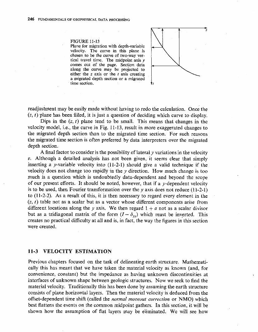
FIGURE 11-13 Plane for migration with depth-variable velocity. The curve in this plane is chosen to be the curve of two-way vertical travel time. The midpoint axis y comes out of the page. Section data along the curve may be projected to either the z axis or the t axis creating a migrated depth section or a migrated time section.

readjustment may be easily made without having to redo the calculation. Once the (2, t) plane has been filled, it is just a question of deciding which curve to display.

Dips in the (2, t ) plane tend to be small. This means that changes in the velocity model, i.e., the curve in Fig. 11-13, result in more exaggerated changes to the migrated depth section than to the migrated time section. For such reasons the migrated time section is often preferred by data interpreters over the migrated depth section.

A final factor to consider is the possibility of lateral y variations in the velocity v. Although a detailed analysis has not been given, it seems clear that simply inserting a y-variable velocity into (11-2-1) should give a valid technique if the velocity does not change too rapidly in the y direction. How much change is too much is a question which is undoubtedly data-dependent and beyond the scope of our present efforts. It should be noted, however, that if a y-dependent velocity is to be used, then Fourier transformation over the y axis does not reduce (1 1-2-1) to (1 1-2-2). As a result of this, it is then necessary to regard every element in the (2, t) table not as a scalar but as a vector whose different components arise from different locations along the y axis. We then regard 1 + a not as a scalar divisor but as a tridiagonal matrix of the form (I - a,,) which must be inverted. This creates no practical difficulty at all and is, in fact, the way the figures in this section were created.

11-3 VELOCITY ESTIMATION

Previous chapters focused on the task of delineating earth structure. Mathemati- cally this has meant that we have taken the material velocity as known (and, for convenience, constant) but the impedance as having unknown discontinuities at interfaces of unknown shape between geologic structures. Now we seek to find the material velocity. Traditionally this has been done by assuming the earth structure consists of plane horizontal layers. Then the material velocity is deduced from the offset-dependent time shift (called the normal moueout correction or NMO) which best flattens the events on the common midpoint gathers. In this section, it will be shown how the assumption of flat layers may be eliminated. We will see how

velocity can be estimated even in an earth consisting of random point scatterers. This can be expected to be useful in fractured zones or even perhaps in " no record " areas. An NR or no record area is one where the best-processed section shows no coherence along the midpoint y coordinate. An area may be NR not only because of poor data quality but also because the geologic structure itself has no continuity. But, as we will see, there is no theoretical reason why material velocity cannot be determined in such an NR area.

Basically, the procedure is to downward-continue both the theoretical downgoing wave and the observed upgoing wave. They are projected back down to the reflectors where their nearly constant ratio should represent the reflection coefficient as a function of offset. If they are projected downwards with an incorrect velocity, the ratio will be an oscillatory function of offset. The task, then, is to find the velocity which gives the best fit of the two waves. It does not matter whether the reflectors have any lateral continuity or not because the fitting is done for variable offset at a fixed midpoint at the reflector depth. When reflectors have no lateral continuity they may be called scatterers. An earth model with randomly located scatterers would produce migrated seismic data which was a random function of (moveout-corrected) time and midpoint but which was a constant function of offset.

It is easy to think of a good means to downward-continue the downgoing waves. From the shot point these waves expand spherically. For a homogeneous medium, we can just write down an analytic solution. For a moderately inhomogeneous medium, we can use the methods of earlier chapters. One problem is that the approximation Q,, = 0 restricts validity to angles of about 15" from the vertical. This is easily improved by transforming from cartesian (x, z) coordinates to polar (r, 0) coordinates. The approximation Q,, z 0 requires rays to stay within 15" of a radius line. Obviously a " stratified media coordinate frame" could be designed to handle even stronger velocity inhomogeneity of that type.

The problem which is more difficult is to find a good coordinate system for the upcoming waves. It took me two years to come up with a practical solution. A hint is provided by observing why, for the downgoing wave, the polar system is preferable to the cartesian system. For a quasi-spherical wave Q,, will be nearly 0, whereas Q,, gets large quickly unless you are directly under the source. Because we deal with equations like Q,, = Q,, or Q,, = Q,,/r2, this means that Q, will generally be small; whereas Q, is small only on the z axis directly under the source. Consequently, the approximation Q,, = 0 is much better than Q,, z 0. Our observation is that the advantage of the (r, 0) coordinates is that the downgoing wave D(r, 0) is nearly independent of the lateral 0 coordinate. What we need is a coordinate frame in which the upcoming wave U is nearly independent of the lateral coordinate. Experienced geophysicists will immediately recognize that normal moveout-corrected data fill this requirement. Normal moveout (NMO) correction is a compression of the time axis on far offset seismograms intended to make the far offset waves arrive at the same (NMO corrected) time as the vertically incident waves. Thus, the partial derivative of the wave field Q with respect to shot-geophone offset at a fixed NMO corrected time should be small.

The closer our data come to those from flat horizontal reflectors in an earth

FIGURE 11-14 Geometry for normal-moveout correction of downward-continued data.

of known velocity the smaller the offset derivative will be. The purpose of a wave equation is to handle the departure from such an idealized situation.

This compression of the time axes of the far offset seismograms is really a coordinate change. The usual definition of NMO correction does not anticipate our desire to project our geophones deeply into the earth. As we project our geophones downward along a ray path we will retain the surface midpoint y and the surface half-oflset h =f /2 as lateral coordinates of the wave field. Lateral derivatives of idealized data should vanish.

Figure 11-14 shows the geometry for normal moveout correction of downward- continued data in homogeneous media of velocity G. The transformation from interpretation variables to observation variables is

(d2 + h2)'l2(2d - Z) t(h, y, d, 2 ) = (1 1-3-lc)

dii

Either algebraic or geometric means yield the inverse transformation

That (1 1-3-2) is indeed inverse to (1 1-3-1) is readily checked by substituting (1 1-3-1) into (1 1-3-2).

In a homogeneous medium of velocity u" we may write the solution for the downgoing wave as a delta function on an expanding circle

The upcoming wave U will be computed in the (h, y, d, z) variables and we want to compare it to the downgoing wave D, expressed by (1 1-3-3) in (g, s, t, z) variables. We can convert D to (h, y, d, z) variables by substitution of (1 1-3-1) into (1 1-3-3); a meaningful simplification arises if we assume the medium velocity u" equals the moveout coordinate frame velocity 6. We get

In this case, the downgoing wave turns out to be independent of the lateral coordinates h and y.

Now let us consider an earth model which contains only a single point scatterer located at (x,, 2,). This scatterer is illuminated by a delta function source located at (s, 0). Excluding horizontally propagating waves, we have for the upcoming wave U(s, g, t , z) an infinitesimal distance above the scatterer

Substituting the transformation (1 1-3-1) at z = d into (1 1-3-5), we obtain

The existence of 6(y -xo) allows us to set y = xo in the other delta function, getting

We now see the central concept that the wave at the reflector in moveout corrected coordinates is indeed independent of the half-offset h. Obviously, the superposition of a random collection of point scatterers will create a migrated wave field which is random in y and d but still constant in the offset h. Indeed, the concept would also seem to be valid even if the scatterers were randomly distributed out of the plane of the section. In three-dimensional space it is only necessary to regard z as the radial distance from the traverse Iine.

The purpose of all this is to estimate velocity; but velocity is needed for the first step, namely the migration. Use of an erroneous velocity in the migration prevents total collapse to a delta function on the midpoint axis. This causes some destructive interference between adjoining midpoints representing some information loss for a random scatterer model but it is of no consequence in a layered earth model (where even the migration itself is unnecessary).

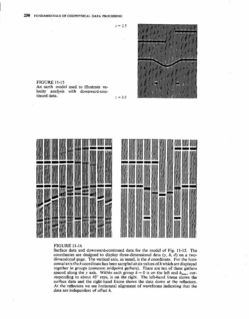
Stephen M. Doherty [Ref. 371 made a calculation to illustrate these concepts. Figure 11-15 shows an earth model. Figure 11-16 shows surface data and downward-continued data for the model.

From the point of view of velocity determination, it is immaterial what coordinate frame is used to downward-continue the observed waveforms. However,


FIGURE 11-15 An earth model used to illustrate velocity analysis with downward-continued data.

FIGURE 1 1-1 6 Surface data and downward-continued data for the model of Fig. 11-15. The coordinates are designed to display three-dimensional data (y, h, d) on a two- dimensional page. The vertical axis, as usual, is the d coordinate. For the horizontal axis the h coordinate has been sampled at six values of h which are displayed together in groups (common midpoint gathers). There are ten of these gathers spaced along the y axis. Within each group h = 0 is on the left and h,,,, corresponding to about 45" rays, is on the right. The left-hand frame shows the surface data and the right-hand frame shows the data down at the reflectors. At the reflectors we see horizontal alignment of waveforms indicating that the data are independent of offset h.

it is convenient to downward-continue these waves in the NMO coordinate frame. This proceeds in a fashion similar to that in our earlier work. To simplify the alge- bra, first note that (1 1-3-2b) and (1 1-3-2c) imply that

The wave equation

in NMO coordinates will take the form

As before, when we square these partial differential operators we will take the coefficients to be constant. This is the high frequency assumption that the wave field changes more rapidly than the coordinate frame. Before we compute all the required derivatives we define a simplifying combination b where

The required derivatives are computed, recalling (1 1-3-6) to be

First we quickly discover that if moveout-correction velocity fi equals media velocity ij, say 5 = 5 = v, then three of the terms in (1 1-3-8) vanish identically. By direct substitution, the reader may verify that

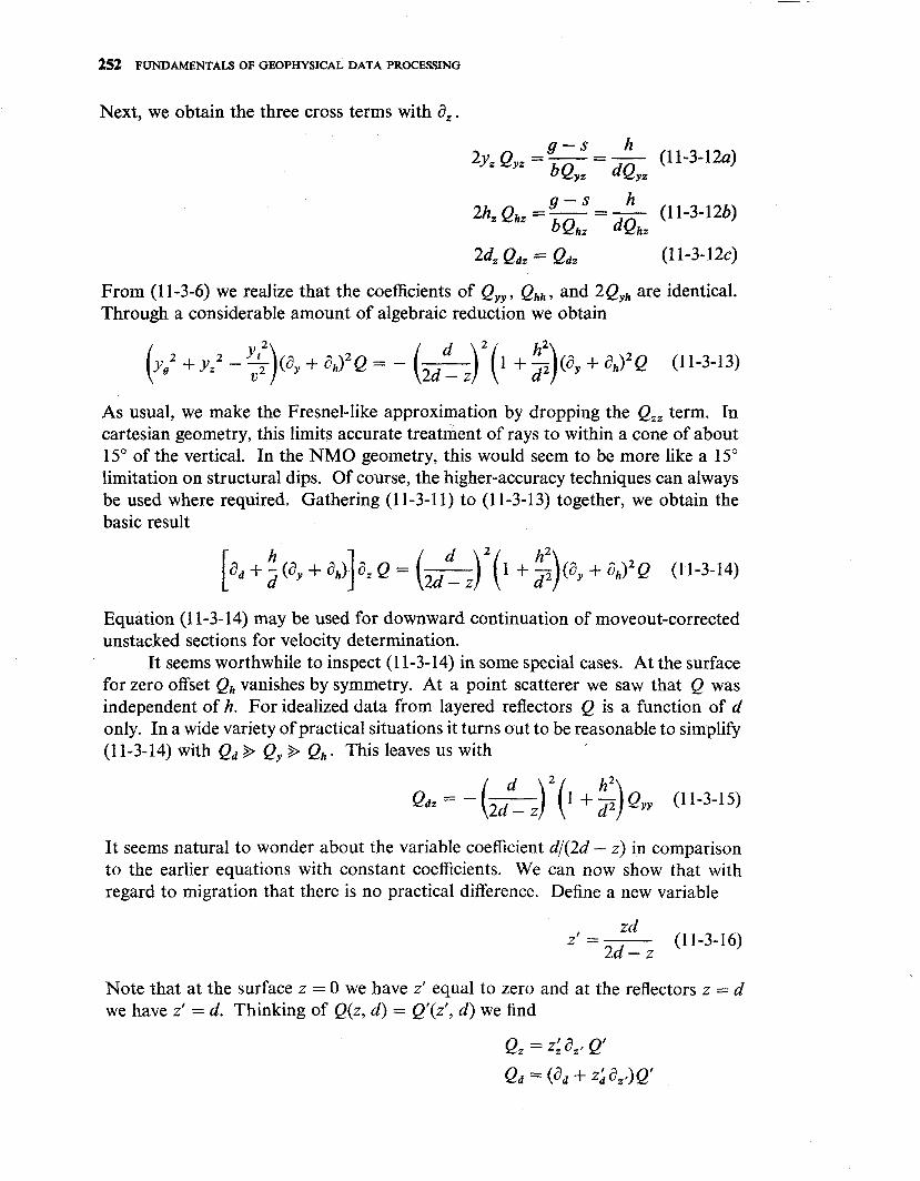
Next, we obtain the three cross terms with 8,.

g - s h 2yz Qyz = - = - (1 1-3- 12a)

bQyz dQyz g - s h

2hz Qh, =- = - (1 1-3-12b) b Qhz dQhz

2dz Qdz = Qdz (1 1-3- 12c)

From (1 1-3-6) we realize that the coefficients of Qyy , Qhh , and 2Qyh are identical. Through a considerable amount of algebraic reduction we obtain

As usual, we make the Fresnel-like approximation by dropping the Qzz term. In cartesian geometry, this limits accurate treatment of rays to within a cone of about 15" of the vertical. In the NMO geometry, this would seem to be more like a 15" limitation on structural dips. Of course, the higher-accuracy techniques can always be used where required. Gathering (1 1-3-1 1) to (1 1-3-13) together, we obtain the basic result

Equation (1 1-3-14) may be used for downward continuation of moveout-corrected unstacked sections for velocity determination.

It seems worthwhile to inspect (1 1-3-14) in some special cases. At the surface for zero offset Qh vanishes by symmetry. At a point scatterer we saw that Q was independent of h. For idealized data from layered reflectors Q is a function of d only. In a wide variety of practical situations it turns out to be reasonable to simplify (1 1-3-14) with Qd 9 Q, + Qh . This leaves us with

It seems natural to wonder about the variable coefficient dl(2d - z) in comparison to the earlier equations with constant coefficients. We can now show that with regard to migration that there is no practical difference. Define a new variable

Note that at the surface z = 0 we have z' equal to zero and at the reflectors z = d we have z' = d. Thinking of Q(z, d) = Qr(zt, d) we find

With these, the left-hand side of (1 1-3-15) becomes

In a Fresnel-like approximation, we drop obtaining

which reduces (1 1-3- 15) to

Q,, (11-3-17)

To justify the factor of 2 which was asserted in Sec. 11-2, we may make another transformation from d to a two-way travel-time coordinate t' given by

which gives

Of course (1 1-3-18) must be integrated from 2' = 0 to z' = t1v'/2. A convenient rescaling of the depth axis is in terms of two-way travel time t" where

This leads to the equation

in which t' is the two-way travel time and t" is the two-way travel-time depth axis which is integrated from the surface t" = 0 to the reflectors at t" = t'.

Strictly speaking, (1 1-3-19) should be applied separately to data of each offset h before the data are summed over offset (stacked). For reasons of economy, the data are often stacked before migration with (11-3-19). In such a compromise, h in (1 1-3-19) is taken as zero or some average value of 2h/ut1 is used.

So far, we have shown that downward-continued, moveout-corrected seismograms will be independent of offset if downward continued with the correct velocity. What we have not seen is how to estimate the velocity error from the downward-continued data. For this we must recognize another important term which has been omitted from the entire analysis. We saw this term in earlier studies of propagation in inhomogeneous media. We must carry through the distinction between media velocity c ( ~ , z) and NMO velocity 6 [generalizable to 6(z)] which was abandoned for the sake of the simplifications beginning at (1 1-3-1 1). Recalling that for small departu~es from layered models, Qd 9 Q, 9 Q,, we see

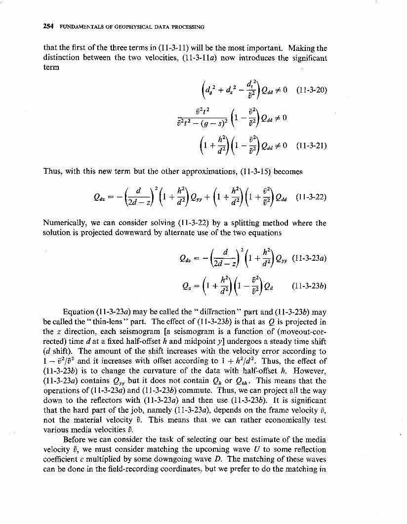
that the first of the three terms in (1 1-3-1 1) will be the most important. Making the distinction between the two velocities, (11-3-lla) now introduces the significant term

Thus, with this new term but the other approximations, (1 1-3-15) becomes

Numerically, we can consider solving (1 1-3-22) by a splitting method where the solution is projected downward by alternate use of the two equations

Equation (1 1-3-23a) may be called the " diffraction" part and (1 1-3-233) may be called the " thin-lens " part. The effect of (1 1-3-23b) is that as Q is projected in the z direction, each seismogram [a seismogram is a function of (moveout-corrected) time d at a fixed half-offset h and midpoint y ] undergoes a steady time shift (d shift). The amount of the shift increases with the velocity error according to 1 - v2/c2 and it increases with offset according to 1 + h2/d2. Thus, the effect of (11-3-238) is to change the curvature of the data with half-offset h. However, (11-3-23a) contains Qyy but it does not contain Qh or Qhh. This means that the operations of (1 1-3-23a) and (1 1-3-23b) commute. Thus, we can project all the way down to the reflectors with (11-3-23a) and then use (11-3-233). It is significant that the hard part of the job, namely (1 1-3-23a), depends on the frame velocity u, not the material velocity u". This means that we can rather economically test various media velocities u".

Before we can consider the task of selecting our best estimate of the media velocity u", we must consider matching the upcoming wave U to some reflection coefficient c multiplied by some downgoing wave D. The matching of these waves can be done in the field-recording coordinates, but we prefer to do the matching in

the NMO coordinate system. First, let us get an expression for the downgoing wave in NMO coordinates. Insert (1 1-3-1) into (1 1-3-3) to obtain

At present, we are not trying to preserve slow magnitude variations [spherical spreading was omitted from (11-3-3)], so we can divide through the argument of the delta function by -4d. Since we are interested in small amounts of variation of 6 from ij the delta function will vanish very near to z = d. Thus, to a good approximation we can substitute z for d i n the coefficient of (1 - c2/ij2), obtaining

where we have defined a time (d) shift function

Now let us return to the task of matching the up- and downgoing wave. We might hope to determine a reflection coefficient, along with some angular dependence, in the form of a power series, for example:

To simplify the sequel we will estimate only the constant term c, by the minimi- zation

min 1 1 [U(Y, 2, h, d) - C(Y, z)D(Y, 2, h, d)12 (1 1-3-28) c h d

The solution is obviously

Because D vanishes almost everywhere, we can gain insight by replacing the double sum by a single sum, specifically for the numerator

Numerator = x x U(y, z, h, d) 6(d - z - s) h d

= x u(y, Z, h, d = z + s(h2, Z, s/a)] (1 1-3-30) h

Letting N denote the number of terms in the offset sum, we get for (1 1-3-29)


Finally, we come to the part of determining the velocity v" which provides the best minimum of U - cD. For this, a computer scan over 5 may be used to find the minimum

min z (U - C D ) ~ = min x (U - c ) ~ ii h d i i h

In practice it is found that rather than minimize the sum squared minus the squared sum it is preferable to maximize the negative logarithm or the semblance ratio

Semblance = ii

(' U)2 < 1 (1 1-3-33) N x U 2 -

The ratio has the advantage of being insensitive to the magnitude of the wave U and lends itself well to displays over a wide range of conditions.

11-4 MULTIPLE REFLECTIONS

Accurate modeling of multiple reflections makes it possible to subtract theoretical multiples from field data, thereby uncovering the more informative, primary reflections. We will first review a simplified layered model for multiple reflections and then modify it for application to a two-dimensionally inhomogeneous earth. We plan to solve both forward and inverse problems. The forward problem is given the two-dimensional spatial distribution of reflection coefficients to find the reflections including diffracted multiples with peglegs. The inverse problem is to deduce the two-dimensional spatial distribution of reflection coefficients from the waves.

The basic idea that we use for the inverse problem is that " reflectors exist at points in the earth where the first arrival of a downgoing wave is time-coincident with an upcoming wave." As a practical matter, we try to choose reflection coefficients which ensure that the upcoming wave vanishes before the onset of the downgoing wave. In Chap. 8 we learned that, for a layered medium, the Z transform polynomial for the downgoing wave D(Z) is minimum-phase. This means that the inverse of D(Z), namely l/D(Z), can be expanded into positive powers of Z and the lead coefficient will be lld,. Consequently, in the nth layer the reflection coefficient at the bottom of the layer is the coefficient of the lowest power of Z in the expansion for Un(Z)/Dn(Z). Our plan is to show that Un(Z)/Dn(Z) is observable at the surface n = 0, and then show how Un+'/Dn+l can be easily computed from Un/Dn. First of all, pressure P and vertical velocity W must be taken as known at the surface for all time.

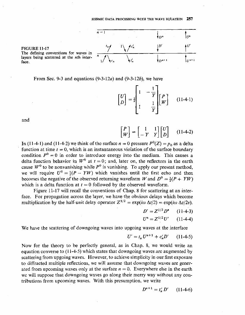
FIGURE 11-17 The defining conventions for waves in

t" layers being scattered at the nth interface.

From Sec. 9-3 and equations (9-3-12a) and (9-3-12b), we have

and

In (1 1-4-1) and (1 1-4-2) we think of the surface n = 0 pressure ~ ' ( 2 ) = p , as a delta function at time t = 0, which is an instantaneous violation of the surface boundary condition PO = 0 in order to introduce energy into the medium. This causes a delta function behavior in WO at t = 0; and, later on, the reflectors in the earth cause WO to be nonvanishing while PO is vanishing. To apply our present method, we will require UO = +(P - YW) which vanishes until the first echo and then becomes the negative of the observed returning waveform Wand Do = f(P + YW) which is a delta function at t = 0 followed by the observed waveform.

Figure 11-17 will recall the conventions of Chap. 8 for scattering at an interface. For propagation across the layer, we have the obvious delays which become multiplication by the half-unit delay operator 2'12 = exp(iw At/2) = exp(io A.212~).

We have the scattering of downgoing waves into upgoing waves at the interface

U' = t, Un+l + CAD' (1 1-4-5)

Now for the theory to be perfectly general, as in Chap. 8, we would write an equation converse to (1 1-4-5) which states that downgoing waves are augmented by scattering from upgoing waves. However, to achieve simplicity in our first exposure to diffracted multiple reflections, we will assume that downgoing waves are gener- ated from upcoming waves only at the surface n = 0. Everywhere else in the earth we will suppose that downgoing waves go along their merry way without any con- tributions from upcoming waves. With this presumption, we write

,258 FUNDAMENTALS OF GEOPHYSICAL DATA PROCESSING

As a practical matter, the assumption we have built into (1 1-4-6) is not a bad one for marine data where the free-surface reflector is by far the strongest reflector. Although a large range of reflection coefficients is found in practice, a common case would be for a sea-floor coefficient of . l and subsurface coefficients of .Ol. With land data, it is often important to account for a lot of absorption and scattering in the near-surface layers.

Anyway, eliminating the D' and U' variables from (1 1-4-3) to (1 1-4-6), we obtain

~ n + l - - t f ~ 1 / 2 ~ 1 1 (1 1-4-7)

Dividing (1 1-4-8) by (1 1-4-7), we achieve a simple relationship for the downward continuation of U/D. It is

To understand this simple recurrence relationship we must recall that the coefficient of Z0 in Un/Dn vanishes (see Fig. 11-17) and that the coefficient of Z in Un/Dn - I is c, = -cn. Thus, the 2 - I multiplier in (1 1-4-9) shifts Un/Dn to have -cn as the coefficient of 2' and then the c, in (1 1-4-9) extinguishes it. Clearly, the downward continuation is so simple that the results can almost be seen as the coefficients of the surface ratio uO(Z)/DO(Z). The only complicating factor is the divisor tit, which gives a monotonically increasing scale factor of l /n ;= , (1 - ck2) to the coefficient of Zn in uO(Z)/DO(Z).

Now let us see how we can generalize these layered-model ideas to a two- dimensionally inhomogeneous earth. The big difference is that upward and downward continuation of waveforms can no longer be accomplished simply by the delay operator 2. We could use (10-5-16) for upward and downward continuation; however, it seems more natural and certainly more economical to use (10-5-17a) and (10-5-18) which are

Equations (11-4-10) and (11-4-11) may be compared with (11-4-7) and (11-4-8). It is apparent that transmission coefficients are not accounted for in (1 1-4-10) and (1 1-4-1 1). That is the sort of thing which is usually unimportant in the analysis of field data, but which can be recovered by a more exhaustive derivation if necessary.

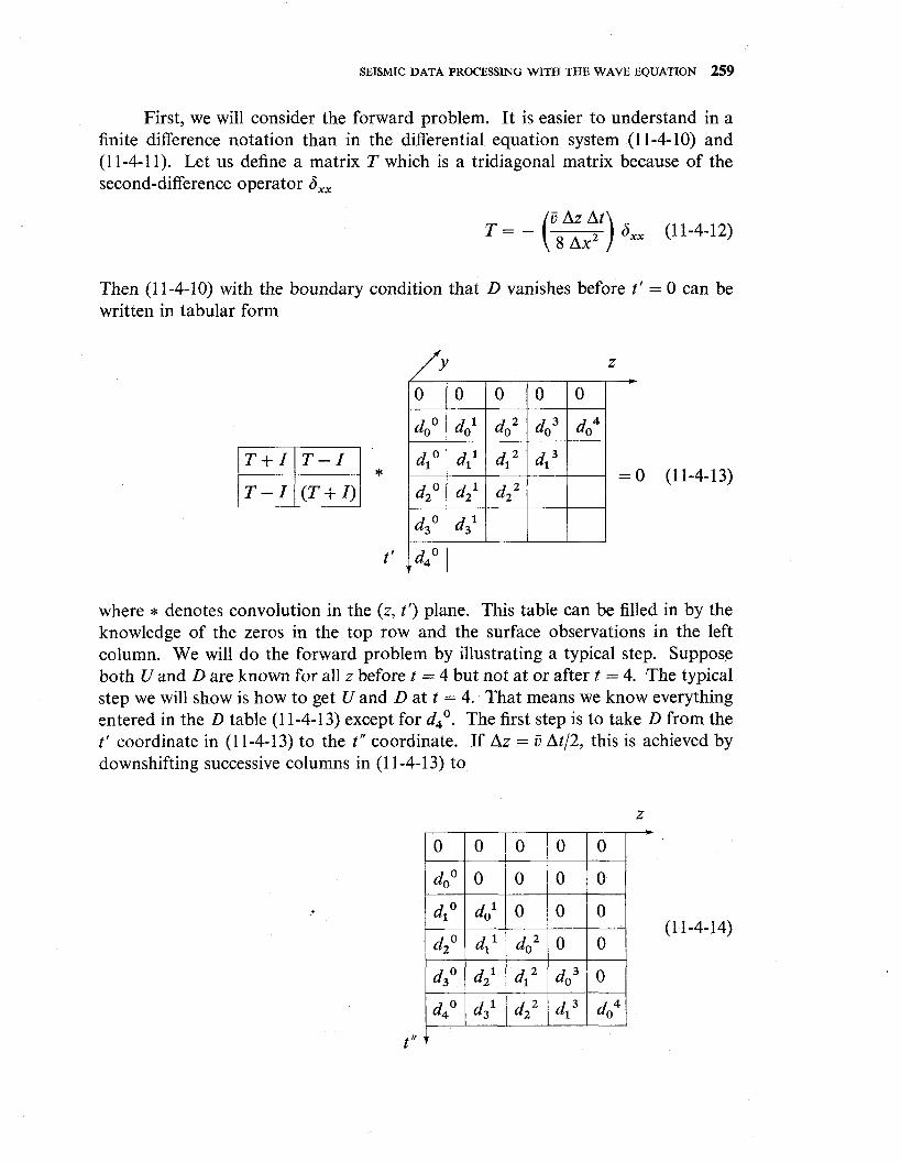
First, we will consider the forward problem. It is easier to understand in a finite difference notation than in the differential equation system (11-4-10) and (11-4-1 1). Let us define a matrix T which is a tridiagonal matrix because of the second-difference operator ax,

Then (1 1-4-10) with the boundary condition that D vanishes before t ' = 0 can be written in tabular form

where * denotes convolution in the (z, t') plane. This table can be filled in by the knowledge of the zeros in the top row and the surface observations in the left column. We will do the forward problem by illustrating a typical step. Suppose both U and D are known for all z before t = 4 but not at or after t = 4. ,The typical step we will show is how to get U and D at t = 4. That means we know everything entered in the D table (1 1-4-13) except for d40. The first step is to take D from the t' coordinate in (1 1-4-1 3) to the t" coordinate. If Az = ij At/2, this is achieved by downshifting successive columns in (1 1-4-13) to

The meaning of the t" coordinate is that if reflection occurs, all elements on a given row of constant t" can contribute to the upcoming wave received at a surface arrival time t". Equation (1 1-4-11) may be rearranged to

(i a, + a,,) ( - u) = c'(x, z)a,D (1 1-4-1 5 )

which can be expressed in tabular form as

In the tabular equation (1 1-4-16) the unknown elements have been left blank. On the right-hand side the reflection coefficients are to be convolved upward into the downgoing wave to create the sources for the upgoing wave. The co entry in the reflection coefficient row is set at zero because we will prescribe the boundary condition dtO = -utO separately. Thus, we see the right-hand side of (11-4-16) is completely known, and the unknowns in the left-hand side may be filled in from right to left, thereby computing the upcoming wave table at t" = 4 for all z. This gives d,', enabling us to go back and fill in another row in the downgoing wave table which enables us to fill another row in the upgoing wave table, ad infinitum.

The inverse calculation proceeds in a similar fashion. Suppose dtO is known for all t and we wish to calculate c; , ci , etc., in a recursive fashion. It is sufficient

SEISMIC DATA PROCESSING WITH THE WAVE EQUATION 261

to show how to compute c;. Suppose we skim off the two left-hand columns of (1 1-4-16). We get

T - I T + I Convolve l&l\ I up

In (1 1-4-17) all the boxes filled by g on the left are given. The boxes with g on the right are readily computable as before. If c; were known, it would be a straightforward task to compute successively . . . , e3 , e, , el, eo . We would be compelled to initialize the computation with an approximation such as e, = 0 for some large N. If the correct value of c; had been used, then we should find that eo vanishes. Since we do not know what value of c; to use, we try c; = + 1 obtaining e,f and we try c; = - 1 obtaining e, . The correct value of c; is the appropriately weighted linear combination

where

which inverts to

reducing (1 1-4- 18) to

or


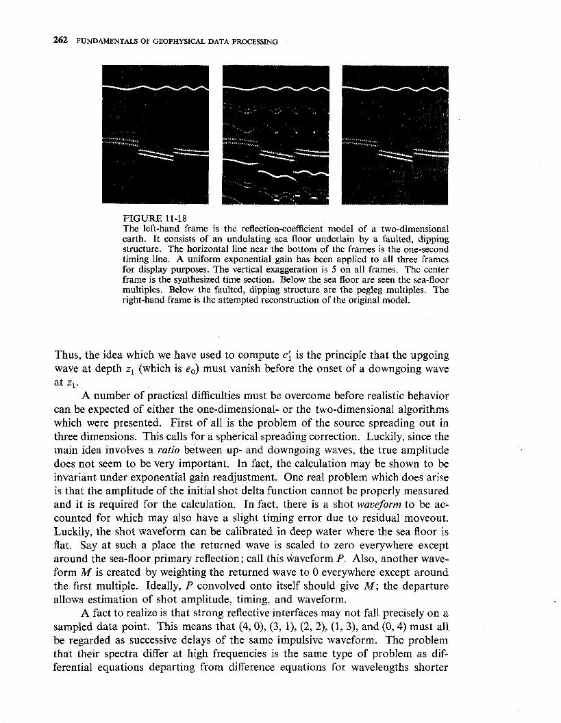
FIGURE 1 1-1 8 The left-hand frame is the reflection-coefficient model of a two-dimensional earth. It consists of an undulating sea floor underlain by a faulted, dipping structure. The horizontal line near the bottom of the frames is the one-second timing line. A uniform exponential gain has been applied to all three frames for display purposes. The vertical exaggeration is 5 on all frames. The center frame is the synthesized time section. Below the sea floor are seen the sea-floor multiples. Below the faulted, dipping structure are the pegleg multiples. The right-hand frame is the attempted reconstruction of the original model.

Thus, the idea which we have used to compute c; is the principle that the upgoing wave at depth z, (which is e,) must vanish before the onset of a downgoing wave at z,.

A number of practical difficulties must be overcome before realistic behavior can be expected of either the one-dimensional- or the two-dimensional algorithms which were presented. First of all is the problem of the source spreading out in three dimensions. This calls for a spherical spreading correction. Luckily, since the main idea involves a ratio between up- and downgoing waves, the true amplitude does not seem to be very important. In fact, the calculation may be shown to be invariant under exponential gain readjustment. One real problem which does arise is that the amplitude of the initial shot delta function cannot be properly measured and it is required for the calculation. In fact, there is a shot waveform to be accounted for which may also have a slight timing error due to residual moveout. Luckily, the shot waveform can be calibrated in deep water where the sea floor is flat. Say at such a place the returned wave is scaled to zero everywhere except around the sea-floor primary reflection; call this daveform P. Also, another waveform M is created by weighting the returned wave to 0 everywhere except around the first multiple. Ideally, P convolved onto itself should give M; the departure allows estimation of shot amplitude, timing, and waveform.

A fact to realize is that strong reflective interfaces may not fall precisely on a sampled data point. This means that (4, O), (3, I), (2, 2), (1, 3), and (0,4) must all be regarded as successive delays of the same impulsive waveform. The problem that their spectra differ at high frequencies is the same type of problem as differential equations departing from difference equations for wavelengths shorter

than about ten sample points. There is no need to model the high frequencies accurately; just be sure to sample the data densely enough. The real problem with high frequencies is keeping them from causing instability. For example, in the calculation of uOIDO = - W(Z)/[~ + W(Z)] it is first necessary to estimate the @ which would be recorded if the shot P/I had been an ideal delta function. Naturally, the high frequencies in w are rather meaningless. The only reason you care about them is that they should not be such as to make 1 + ~nonminimum-phase which would prevent the division. In this case, the high frequencies can be filtered out from @ and the divisor will tend toward a positive real function. Don C . Riley [Ref. 381 has established that these various practical difficulties can be overcome and Fig. 11-18 shows an example of one of his calculations.

seismic data processing with the wave …sep · seismic data processing with the wave equation the...

Documents