Converted-wave seismic imaging: Amplitude-balancingsource-independent imaging conditions

Andrey H. Shabelansky1, Alison Malcolm2, and Michael Fehler3

ABSTRACT

We have developed crosscorrelational and deconvolu-tional forms of a source-independent converted-wave imag-ing condition (SICW-IC) and show the relationship betweenthem using a concept of conversion ratio coefficient, a con-cept that we developed through reflection, transmission, andconversion coefficients. We applied the SICW-ICs to a twohalf-space model and the synthetic Marmousi I and II mod-els and show the sensitivity of the SICW-ICs to incorrectwave speed models. We also compare the SICW-ICs andsource-dependent elastic reverse time migration. The resultsof SICW-ICs highlight the improvements in spatial resolu-tion and amplitude balancing with the deconvolutionalforms. This is an attractive alternative to active and passivesource elastic imaging.

INTRODUCTION

Seismic imaging of the earth’s interior is important in explorationand global seismology. It produces images of subsurface discontinu-ities associated with impedance contrasts through reflection, trans-mission, or conversion coefficients of propagating waves. One ofthe pioneering studies on seismic imaging is presented by Claerbout(1971) who introduces the concept of a reflective imaging condition(IC). This concept is based on the fundamental assumption that theacquisition/survey geometry is well-known: The source and receiverlocations are known, and seismic waves can be numerically propa-gated from these locations. This imaging condition has been exten-sively investigated for the past five decades with algorithms for post

and prestack migrations, such as the survey sinking migration(Claerbout, 1985; Popovici, 1996), Kirchhoff-type migration(Schneider, 1978; Bleistein, 1987), shot profile migration (Stoffaet al., 1990), and reverse time migration (Baysal et al., 1983; Changand McMechan, 1994). However, when source information is notavailable, seismic images cannot be constructed using Claerbout’sapproach. An alternative approach is to use interference between dif-ferent wave types propagated backward in time from receiver loca-tions only (Nihei et al., 2001; Xiao and Leaney, 2010; Brytic et al.,2012; Shang et al., 2012; Shabelansky et al., 2013a, 2014). We callthis imaging condition the source-independent converted-wave imag-ing condition (SICW-IC). We discuss the physical meaning of theSICW-IC and present an amplitude-balancing approach for SICWimaging.This paper is divided into three parts. In the first part, we review the

relationship between Claerbout (1971) and SICW-ICs with reflection,transmission, and conversion coefficients. In the second part, we in-troduce the concept of conversion ratio coefficients (CRCs) and weshow how to associate them with different forms of SICW-IC. In thefinal part, we present numerical tests of different forms of SICW-ICapplied to a two half-space model and the synthetic Marmousi I andII models. We also show the sensitivity of the SICW-ICs to wavespeed variations and present a comparison between the SICW-ICsand source-dependent elastic reverse time migration (RTM).

RELATIONSHIP BETWEEN IMAGINGCONDITIONS ANDREFLECTION, TRANSMISSION,

AND CONVERSION COEFFICIENTS

In this section, we present four forms of a source-independentconverted-wave imaging condition following the approach ofClaerbout (1971) for the standard imaging condition.

First presented at the EAGE 2015 Annual Meeting (Shabelansky et al., 2015a).Manuscript received by the Editor 10 March 2015; revised manuscript received 18 October 2016; published online 7 February 2017.

1Formerly Massachusetts Institute of Technology, Department of Earth, Atmospheric and Planetary Sciences, Earth Resources Laboratory, Cambridge,Massachusetts, USA; presently Chevron, Houston, Texas, USA. E-mail: andreys@alum.mit.edu.

2Formerly Massachusetts Institute of Technology, Department of Earth, Atmospheric and Planetary Sciences, Earth Resources Laboratory, Cambridge,Massachusetts, USA; presently Memorial University of Newfoundland, Earth Sciences Department, Newfoundland, Canada. E-mail: amalcolm@mun.ca.

3Massachusetts Institute of Technology, Department of Earth, Atmospheric and Planetary Sciences, Earth Resources Laboratory, Cambridge, Massachusetts,USA. E-mail: fehler@mit.edu.

© 2017 Society of Exploration Geophysicists. All rights reserved.

S99

GEOPHYSICS, VOL. 82, NO. 2 (MARCH-APRIL 2017); P. S99–S109, 13 FIGS.10.1190/GEO2015-0167.1

Dow

nloa

ded

06/2

3/17

to 1

34.1

53.3

7.12

8. R

edis

trib

utio

n su

bjec

t to

SEG

lice

nse

or c

opyr

ight

; see

Ter

ms

of U

se a

t http

://lib

rary

.seg

.org

/

Standard imaging condition

The relationship between the reflection (or reflection conversion)coefficients R associated with impedance contrasts (see Figure 1a),is defined as the ratio between the pure reflected (or reflected con-verted) and the incident wavefields u:

RPP ¼urPPuiP

; RPS ¼urPSuiP

; (1)

and for the transmission (or transmission conversion) coefficients Tas the ratio between the pure transmitted (or transmitted converted)and the incident wavefields:

TPP ¼utPPuiP

; TPS ¼utPSuiP

: (2)

For simplicity we omit the vector notation of the wavefield u (e.g.,displacement, particle velocity, or acceleration) and the spatial andtime indices. Superscripts i, r, and t refer to the incident, reflected,and transmitted waves, respectively, and subscripts P and S denotethe wave type, P and/or S. The wavefields urPS and u

tPS are called the

P to S reflected converted and transmitted converted, respectively.The imaging condition in Claerbout (1971) approximates RPP,

where the incident wavefield is calculated by forward propagationin time from the source and is often called the source wavefield, andthe reflected (or reflected-converted) wavefield is calculated byback propagation in time from the receivers and is called thereceiver wavefield. The incident wavefield in the denominator of

equations 1 and 2 can be zero. Many studies have investigatedhow to avoid the division by zero and suggest different solutions(Valenciano and Biondi, 2003; Kaelin and Guitton, 2006; Chatto-padhyay and McMechan, 2008; Schleicher et al., 2008). One sol-ution is to multiply the numerator and denominator by thedenominator and to add a small number to the denominator (Valen-ciano and Biondi, 2003). Thus, for equation 1, we obtain

IDPP ¼ uiPurPP

ðuiPÞ2 þ ϵ2; IDPS ¼ uiPu

rPS

ðuiPÞ2 þ ϵ2; (3)

where I is the calculated image and ϵ2 is a small number. This formis called a deconvolutional imaging condition, denoted with thesuperscript D. The results obtained with this imaging condition de-pend strongly on the choice of ϵ2, which changes with the data dueto illumination and noise, and the image may still be unstable. As analternative to the deconvolutional imaging condition, Claerbout(1971) also introduces the crosscorrelational imaging conditionby taking only the numerator of equation 3 giving

ICPP ¼ uiPurPP; ICPS ¼ uiPu

rPS; (4)

where the superscript C refers to crosscorrelation. Unlike the de-convolutional imaging condition that has no units just like the re-flection and transmission (or reflection conversion and transmissionconversion) coefficients, the crosscorrelational imaging conditionhas the squared units of the wavefields that form the image. Fig-ure 1b shows schematically the application of the concept of the

imaging condition between forward-propagating(incident) P and backward-propagating (re-flected) P wavefields, and in Figure 1c betweenforward-propagating (incident) P and backward-propagating (reflected-converted) S wavefields.Note that with Claerbout (1971) imaging condi-tion, only one reflected or reflected-convertedwavefield (i.e., either PP or PS) is used at a timeduring the propagation and the other wave type,marked with the gray line, is not used.

Source-independent converted-waveimaging condition

The source-independent converted-wave imag-ing condition uses both back-propagated wave-fields simultaneously (see Figure 1d) in the cross-correlational form as

IC ¼ urPPurPS: (5)

The source location, marked with the star in Fig-ure 1d, is not used for the SICW-IC because we useonly the reflected and reflected-converted wave-fields (i.e., the incident wavefield marked withthe gray line is not used). Moreover, the source lo-cation can be anywhere along the gray lines in Fig-ure 2, which makes SICW-IC applicable to activeand passive seismic data. The sources along thesegray lines can, in general, be outside of the com-putational grid and the image is constructed only in

a) c)

b) d)

Figure 1. Schematics illustrating (a) elastic-wave propagation that samples a point (bluedot) on a reflector with an incident P-wave, (b) imaging of the reflection point usingClaerbout’s imaging condition with forward- and backward-propagating P-waves, andwith (c) forward-propagating P-wave and backward-propagating S-wave. (d) SICW-ICwith P and S backward-propagating waves. The red arrows in panels (b-d) indicate thedirection of the propagating waves that form an image. The gray lines mark the availablewave types that are not used in the image construction. Although the source information,marked with a star, indicates the origin of the waves, the image obtained with SICW-ICin panel (d) uses receiver information only.

S100 Shabelansky et al.

Dow

nloa

ded

06/2

3/17

to 1

34.1

53.3

7.12

8. R

edis

trib

utio

n su

bjec

t to

SEG

lice

nse

or c

opyr

ight

; see

Ter

ms

of U

se a

t http

://lib

rary

.seg

.org

/

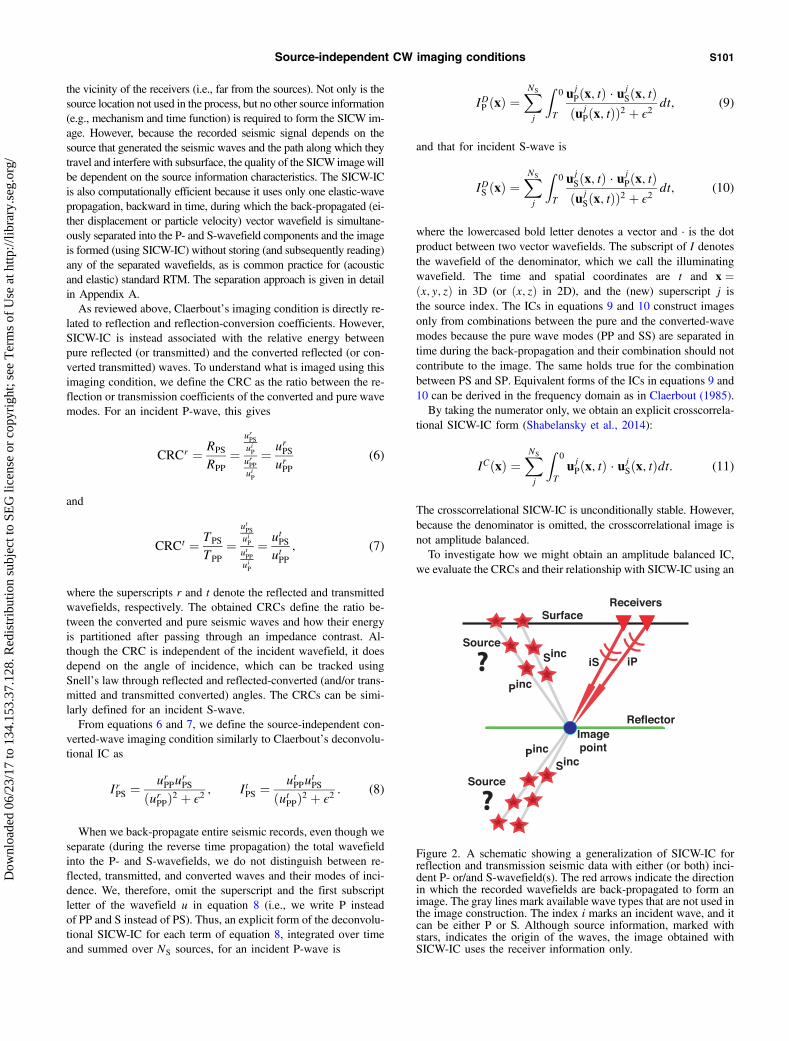
the vicinity of the receivers (i.e., far from the sources). Not only is thesource location not used in the process, but no other source information(e.g., mechanism and time function) is required to form the SICW im-age. However, because the recorded seismic signal depends on thesource that generated the seismic waves and the path along which theytravel and interfere with subsurface, the quality of the SICW imagewillbe dependent on the source information characteristics. The SICW-ICis also computationally efficient because it uses only one elastic-wavepropagation, backward in time, during which the back-propagated (ei-ther displacement or particle velocity) vector wavefield is simultane-ously separated into the P- and S-wavefield components and the imageis formed (using SICW-IC) without storing (and subsequently reading)any of the separated wavefields, as is common practice for (acousticand elastic) standard RTM. The separation approach is given in detailin Appendix A.As reviewed above, Claerbout’s imaging condition is directly re-

lated to reflection and reflection-conversion coefficients. However,SICW-IC is instead associated with the relative energy betweenpure reflected (or transmitted) and the converted reflected (or con-verted transmitted) waves. To understand what is imaged using thisimaging condition, we define the CRC as the ratio between the re-flection or transmission coefficients of the converted and pure wavemodes. For an incident P-wave, this gives

CRCr ¼ RPS

RPP

¼urPS

uiP

urPP

uiP

¼ urPSurPP

(6)

and

CRCt ¼ TPS

TPP

¼utPS

uiP

utPP

uiP

¼ utPSutPP

; (7)

where the superscripts r and t denote the reflected and transmittedwavefields, respectively. The obtained CRCs define the ratio be-tween the converted and pure seismic waves and how their energyis partitioned after passing through an impedance contrast. Al-though the CRC is independent of the incident wavefield, it doesdepend on the angle of incidence, which can be tracked usingSnell’s law through reflected and reflected-converted (and/or trans-mitted and transmitted converted) angles. The CRCs can be simi-larly defined for an incident S-wave.From equations 6 and 7, we define the source-independent con-

verted-wave imaging condition similarly to Claerbout’s deconvolu-tional IC as

IrPS ¼urPPu

rPS

ðurPPÞ2 þ ϵ2; ItPS ¼ utPPu

tPS

ðutPPÞ2 þ ϵ2: (8)

When we back-propagate entire seismic records, even though weseparate (during the reverse time propagation) the total wavefieldinto the P- and S-wavefields, we do not distinguish between re-flected, transmitted, and converted waves and their modes of inci-dence. We, therefore, omit the superscript and the first subscriptletter of the wavefield u in equation 8 (i.e., we write P insteadof PP and S instead of PS). Thus, an explicit form of the deconvolu-tional SICW-IC for each term of equation 8, integrated over timeand summed over NS sources, for an incident P-wave is

IDP ðxÞ ¼XNS

j

Z0

T

ujPðx; tÞ · ujSðx; tÞðujPðx; tÞÞ2 þ ϵ2

dt; (9)

and that for incident S-wave is

IDS ðxÞ ¼XNS

j

Z0

T

ujSðx; tÞ · ujPðx; tÞðujSðx; tÞÞ2 þ ϵ2

dt; (10)

where the lowercased bold letter denotes a vector and · is the dotproduct between two vector wavefields. The subscript of I denotesthe wavefield of the denominator, which we call the illuminatingwavefield. The time and spatial coordinates are t and x ¼ðx; y; zÞ in 3D (or ðx; zÞ in 2D), and the (new) superscript j isthe source index. The ICs in equations 9 and 10 construct imagesonly from combinations between the pure and the converted-wavemodes because the pure wave modes (PP and SS) are separated intime during the back-propagation and their combination should notcontribute to the image. The same holds true for the combinationbetween PS and SP. Equivalent forms of the ICs in equations 9 and10 can be derived in the frequency domain as in Claerbout (1985).By taking the numerator only, we obtain an explicit crosscorrela-

tional SICW-IC form (Shabelansky et al., 2014):

ICðxÞ ¼XNS

j

Z0

TujPðx; tÞ · ujSðx; tÞdt: (11)

The crosscorrelational SICW-IC is unconditionally stable. However,because the denominator is omitted, the crosscorrelational image isnot amplitude balanced.To investigate how we might obtain an amplitude balanced IC,

we evaluate the CRCs and their relationship with SICW-IC using an

Figure 2. A schematic showing a generalization of SICW-IC forreflection and transmission seismic data with either (or both) inci-dent P- or/and S-wavefield(s). The red arrows indicate the directionin which the recorded wavefields are back-propagated to form animage. The gray lines mark available wave types that are not used inthe image construction. The index i marks an incident wave, and itcan be either P or S. Although source information, marked withstars, indicates the origin of the waves, the image obtained withSICW-IC uses the receiver information only.

Source-independent CW imaging conditions S101

Dow

nloa

ded

06/2

3/17

to 1

34.1

53.3

7.12

8. R

edis

trib

utio

n su

bjec

t to

SEG

lice

nse

or c

opyr

ight

; see

Ter

ms

of U

se a

t http

://lib

rary

.seg

.org

/

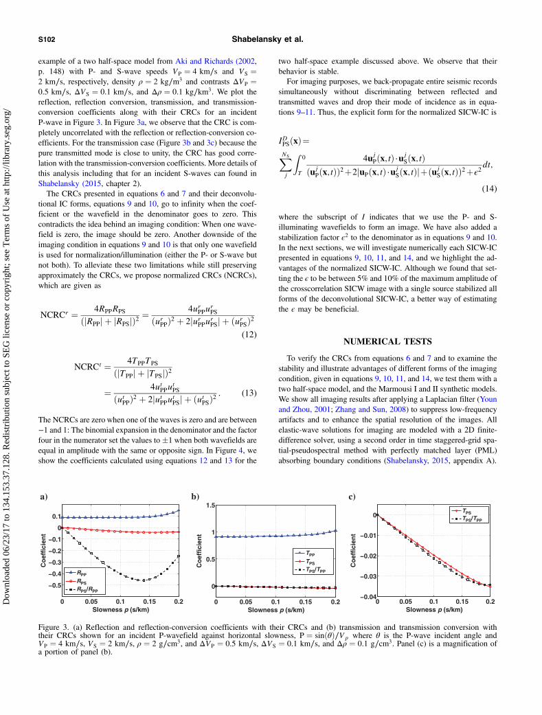
example of a two half-space model from Aki and Richards (2002,p. 148) with P- and S-wave speeds VP ¼ 4 km∕s and VS ¼2 km∕s, respectively, density ρ ¼ 2 kg∕m3 and contrasts ΔVP ¼0.5 km∕s, ΔVS ¼ 0.1 km∕s, and Δρ ¼ 0.1 kg∕km3. We plot thereflection, reflection conversion, transmission, and transmission-conversion coefficients along with their CRCs for an incidentP-wave in Figure 3. In Figure 3a, we observe that the CRC is com-pletely uncorrelated with the reflection or reflection-conversion co-efficients. For the transmission case (Figure 3b and 3c) because thepure transmitted mode is close to unity, the CRC has good corre-lation with the transmission-conversion coefficients. More details ofthis analysis including that for an incident S-waves can found inShabelansky (2015, chapter 2).The CRCs presented in equations 6 and 7 and their deconvolu-

tional IC forms, equations 9 and 10, go to infinity when the coef-ficient or the wavefield in the denominator goes to zero. Thiscontradicts the idea behind an imaging condition: When one wave-field is zero, the image should be zero. Another downside of theimaging condition in equations 9 and 10 is that only one wavefieldis used for normalization/illumination (either the P- or S-wave butnot both). To alleviate these two limitations while still preservingapproximately the CRCs, we propose normalized CRCs (NCRCs),which are given as

NCRCr ¼ 4RPPRPS

ðjRPPj þ jRPSjÞ2¼ 4urPPu

rPS

ðurPPÞ2 þ 2jurPPurPSj þ ðurPSÞ2(12)

NCRCt ¼ 4TPPTPS

ðjTPPj þ jTPSjÞ2

¼ 4utPPutPS

ðutPPÞ2 þ 2jutPPutPSj þ ðutPSÞ2: (13)

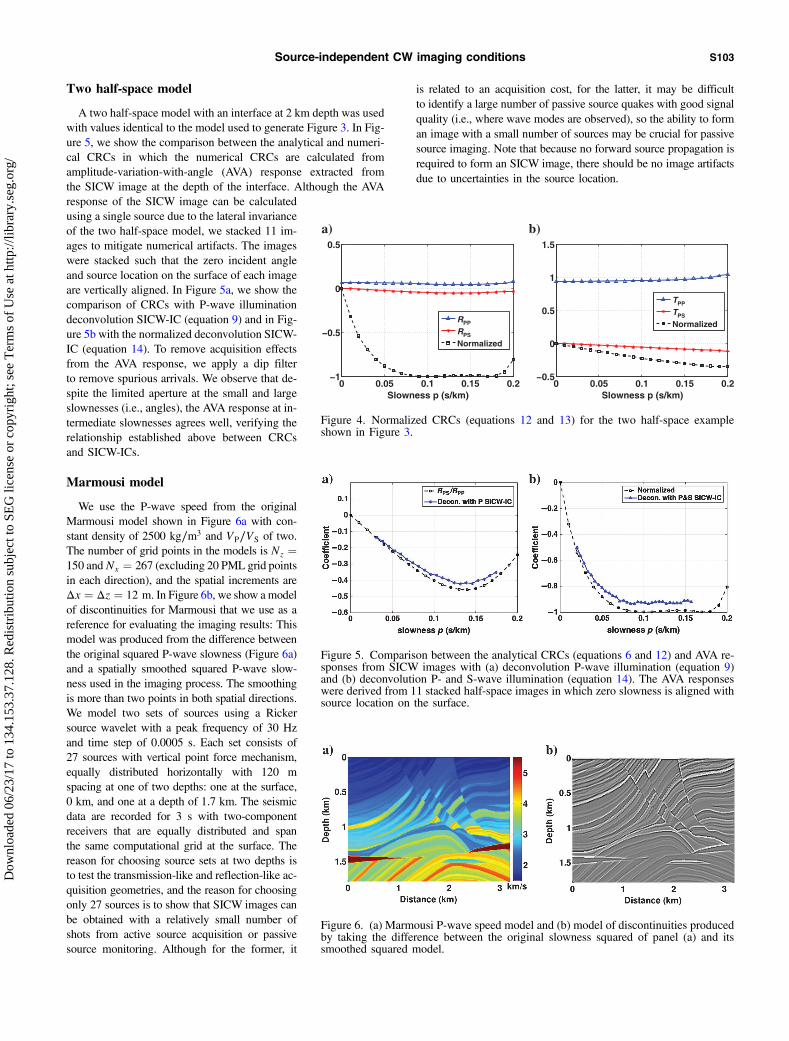
The NCRCs are zero when one of the waves is zero and are between−1 and 1: The binomial expansion in the denominator and the factorfour in the numerator set the values to �1when both wavefields areequal in amplitude with the same or opposite sign. In Figure 4, weshow the coefficients calculated using equations 12 and 13 for the

two half-space example discussed above. We observe that theirbehavior is stable.For imaging purposes, we back-propagate entire seismic records

simultaneously without discriminating between reflected andtransmitted waves and drop their mode of incidence as in equa-tions 9–11. Thus, the explicit form for the normalized SICW-IC is

IDPSðxÞ¼XNS

j

Z0

T

4ujPðx;tÞ ·ujSðx;tÞðujPðx;tÞÞ2þ2juPðx;tÞ ·ujSðx;tÞjþðujSðx;tÞÞ2þϵ2

dt;

(14)

where the subscript of I indicates that we use the P- and S-illuminating wavefields to form an image. We have also added astabilization factor ϵ2 to the denominator as in equations 9 and 10.In the next sections, we will investigate numerically each SICW-ICpresented in equations 9, 10, 11, and 14, and we highlight the ad-vantages of the normalized SICW-IC. Although we found that set-ting the ϵ to be between 5% and 10% of the maximum amplitude ofthe crosscorrelation SICW image with a single source stabilized allforms of the deconvolutional SICW-IC, a better way of estimatingthe ϵ may be beneficial.

NUMERICAL TESTS

To verify the CRCs from equations 6 and 7 and to examine thestability and illustrate advantages of different forms of the imagingcondition, given in equations 9, 10, 11, and 14, we test them with atwo half-space model, and the Marmousi I and II synthetic models.We show all imaging results after applying a Laplacian filter (Younand Zhou, 2001; Zhang and Sun, 2008) to suppress low-frequencyartifacts and to enhance the spatial resolution of the images. Allelastic-wave solutions for imaging are modeled with a 2D finite-difference solver, using a second order in time staggered-grid spa-tial-pseudospectral method with perfectly matched layer (PML)absorbing boundary conditions (Shabelansky, 2015, appendix A).

0 0.05 0.1 0.15 0.2

−0.5

−0.4

−0.3

−0.2

−0.1

0

0.1

Slowness p (s/km)

Co

effi

cien

t

RPP

RPS

RPS/RPP

0 0.05 0.1 0.15 0.2

0

0.5

1

1.5

Slowness p (s/km)

Co

effi

cien

t

TPP

TPS

TPS/TPP

0 0.05 0.1 0.15 0.2−0.04

−0.03

−0.02

−0.01

0

Slowness p (s/km)

Co

effi

cien

t

TPSTPS/TPP

a) b) c)

Figure 3. (a) Reflection and reflection-conversion coefficients with their CRCs and (b) transmission and transmission conversion withtheir CRCs shown for an incident P-wavefield against horizontal slowness, P ¼ sinðθÞ∕Vp where θ is the P-wave incident angle andVP ¼ 4 km∕s, VS ¼ 2 km∕s, ρ ¼ 2 g∕cm3, and ΔVP ¼ 0.5 km∕s, ΔVS ¼ 0.1 km∕s, and Δρ ¼ 0.1 g∕cm3. Panel (c) is a magnification ofa portion of panel (b).

S102 Shabelansky et al.

Dow

nloa

ded

06/2

3/17

to 1

34.1

53.3

7.12

8. R

edis

trib

utio

n su

bjec

t to

SEG

lice

nse

or c

opyr

ight

; see

Ter

ms

of U

se a

t http

://lib

rary

.seg

.org

/

Two half-space model

A two half-space model with an interface at 2 km depth was usedwith values identical to the model used to generate Figure 3. In Fig-ure 5, we show the comparison between the analytical and numeri-cal CRCs in which the numerical CRCs are calculated fromamplitude-variation-with-angle (AVA) response extracted fromthe SICW image at the depth of the interface. Although the AVAresponse of the SICW image can be calculatedusing a single source due to the lateral invarianceof the two half-space model, we stacked 11 im-ages to mitigate numerical artifacts. The imageswere stacked such that the zero incident angleand source location on the surface of each imageare vertically aligned. In Figure 5a, we show thecomparison of CRCs with P-wave illuminationdeconvolution SICW-IC (equation 9) and in Fig-ure 5b with the normalized deconvolution SICW-IC (equation 14). To remove acquisition effectsfrom the AVA response, we apply a dip filterto remove spurious arrivals. We observe that de-spite the limited aperture at the small and largeslownesses (i.e., angles), the AVA response at in-termediate slownesses agrees well, verifying therelationship established above between CRCsand SICW-ICs.

Marmousi model

We use the P-wave speed from the originalMarmousi model shown in Figure 6a with con-stant density of 2500 kg∕m3 and VP∕VS of two.The number of grid points in the models is Nz ¼150 andNx ¼ 267 (excluding 20 PML grid pointsin each direction), and the spatial increments areΔx ¼ Δz ¼ 12 m. In Figure 6b, we show amodelof discontinuities for Marmousi that we use as areference for evaluating the imaging results: Thismodel was produced from the difference betweenthe original squared P-wave slowness (Figure 6a)and a spatially smoothed squared P-wave slow-ness used in the imaging process. The smoothingis more than two points in both spatial directions.We model two sets of sources using a Rickersource wavelet with a peak frequency of 30 Hzand time step of 0.0005 s. Each set consists of27 sources with vertical point force mechanism,equally distributed horizontally with 120 mspacing at one of two depths: one at the surface,0 km, and one at a depth of 1.7 km. The seismicdata are recorded for 3 s with two-componentreceivers that are equally distributed and spanthe same computational grid at the surface. Thereason for choosing source sets at two depths isto test the transmission-like and reflection-like ac-quisition geometries, and the reason for choosingonly 27 sources is to show that SICW images canbe obtained with a relatively small number ofshots from active source acquisition or passivesource monitoring. Although for the former, it

is related to an acquisition cost, for the latter, it may be difficultto identify a large number of passive source quakes with good signalquality (i.e., where wave modes are observed), so the ability to forman image with a small number of sources may be crucial for passivesource imaging. Note that because no forward source propagation isrequired to form an SICW image, there should be no image artifactsdue to uncertainties in the source location.

Figure 5. Comparison between the analytical CRCs (equations 6 and 12) and AVA re-sponses from SICW images with (a) deconvolution P-wave illumination (equation 9)and (b) deconvolution P- and S-wave illumination (equation 14). The AVA responseswere derived from 11 stacked half-space images in which zero slowness is aligned withsource location on the surface.

Figure 6. (a) Marmousi P-wave speed model and (b) model of discontinuities producedby taking the difference between the original slowness squared of panel (a) and itssmoothed squared model.

0 0.05 0.1 0.15 0.2−1

−0.5

0

0.5

Slowness p (s/km)

RPP

RPS

Normalized

0 0.05 0.1 0.15 0.2−0.5

0

0.5

1

1.5

Slowness p (s/km)

TPP

TPS

Normalized

a) b)

Figure 4. Normalized CRCs (equations 12 and 13) for the two half-space exampleshown in Figure 3.

Source-independent CW imaging conditions S103

Dow

nloa

ded

06/2

3/17

to 1

34.1

53.3

7.12

8. R

edis

trib

utio

n su

bjec

t to

SEG

lice

nse

or c

opyr

ight

; see

Ter

ms

of U

se a

t http

://lib

rary

.seg

.org

/

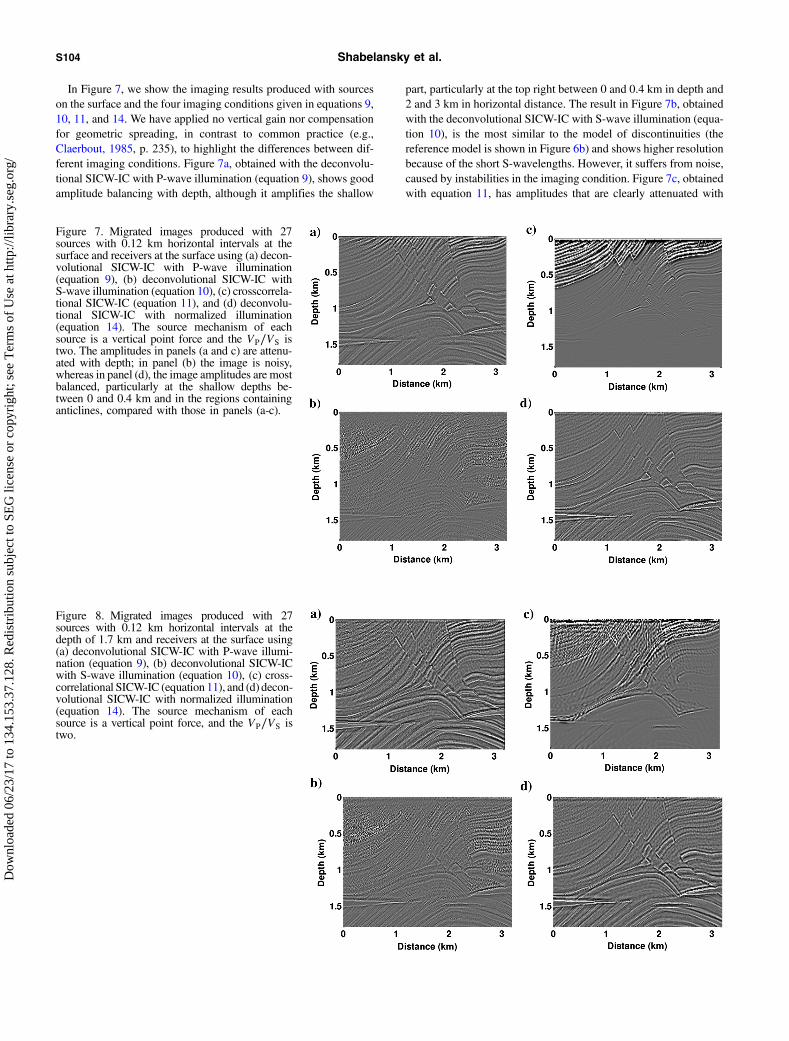
In Figure 7, we show the imaging results produced with sourceson the surface and the four imaging conditions given in equations 9,10, 11, and 14. We have applied no vertical gain nor compensationfor geometric spreading, in contrast to common practice (e.g.,Claerbout, 1985, p. 235), to highlight the differences between dif-ferent imaging conditions. Figure 7a, obtained with the deconvolu-tional SICW-IC with P-wave illumination (equation 9), shows goodamplitude balancing with depth, although it amplifies the shallow

part, particularly at the top right between 0 and 0.4 km in depth and2 and 3 km in horizontal distance. The result in Figure 7b, obtainedwith the deconvolutional SICW-IC with S-wave illumination (equa-tion 10), is the most similar to the model of discontinuities (thereference model is shown in Figure 6b) and shows higher resolutionbecause of the short S-wavelengths. However, it suffers from noise,caused by instabilities in the imaging condition. Figure 7c, obtainedwith equation 11, has amplitudes that are clearly attenuated with

Figure 7. Migrated images produced with 27sources with 0.12 km horizontal intervals at thesurface and receivers at the surface using (a) decon-volutional SICW-IC with P-wave illumination(equation 9), (b) deconvolutional SICW-IC withS-wave illumination (equation 10), (c) crosscorrela-tional SICW-IC (equation 11), and (d) deconvolu-tional SICW-IC with normalized illumination(equation 14). The source mechanism of eachsource is a vertical point force and the VP∕VS istwo. The amplitudes in panels (a and c) are attenu-ated with depth; in panel (b) the image is noisy,whereas in panel (d), the image amplitudes are mostbalanced, particularly at the shallow depths be-tween 0 and 0.4 km and in the regions containinganticlines, compared with those in panels (a-c).

Figure 8. Migrated images produced with 27sources with 0.12 km horizontal intervals at thedepth of 1.7 km and receivers at the surface using(a) deconvolutional SICW-IC with P-wave illumi-nation (equation 9), (b) deconvolutional SICW-ICwith S-wave illumination (equation 10), (c) cross-correlational SICW-IC (equation 11), and (d) decon-volutional SICW-IC with normalized illumination(equation 14). The source mechanism of eachsource is a vertical point force, and the VP∕VS istwo.

S104 Shabelansky et al.

Dow

nloa

ded

06/2

3/17

to 1

34.1

53.3

7.12

8. R

edis

trib

utio

n su

bjec

t to

SEG

lice

nse

or c

opyr

ight

; see

Ter

ms

of U

se a

t http

://lib

rary

.seg

.org

/

depth. The image in Figure 7d produced by equation 14 is similar toFigure 7a. However, although certain small-scale interface conti-nuities are lost, the amplitudes in Figure 7d are considerably betterbalanced and have better spatial resolution with depth when usingP- and S-illuminating wavefields, compared with those in Fig-ure 7a–7c (see particularly the shallow region between 0 and0.4 km in depth, and the deep region of anticlines).In Figure 8, we present images generated with sources at a depth

of 1.7 km. We observe again that the image obtained with the cross-correlational SICW-IC has poorer amplitude recovery comparedwith those produced with the deconvolutional SICW-ICs. Alsothe image with the normalized illumination, Figure 8d has ampli-tudes balanced most similarly to that of the reference model(Figure 6b).As mentioned above, Figures 7 and 8 were obtained with a small

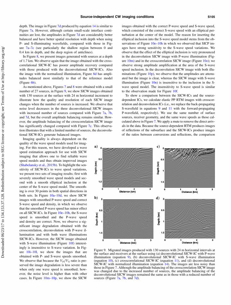
number of 27 sources, in Figure 9, we show SICW images obtainedwith 130 sources at the surface with 24 m horizontal increment toillustrate how the quality and resolution of each SICW imagechanges when the number of sources is increased. We observe thatnoise level decreases in the three deconvolutional SICW imageswith increased number of sources compared with Figure 7a, 7b,and 7d, but the overall amplitude balancing remains similar. How-ever, the amplitude balancing of the crosscorrelation SICW imagehas significantly changed compared with Figure 7c. This observa-tion illustrates that with a limited number of sources, the deconvolu-tional SICW-ICs generate balanced images.Imaging quality is always dependent on the

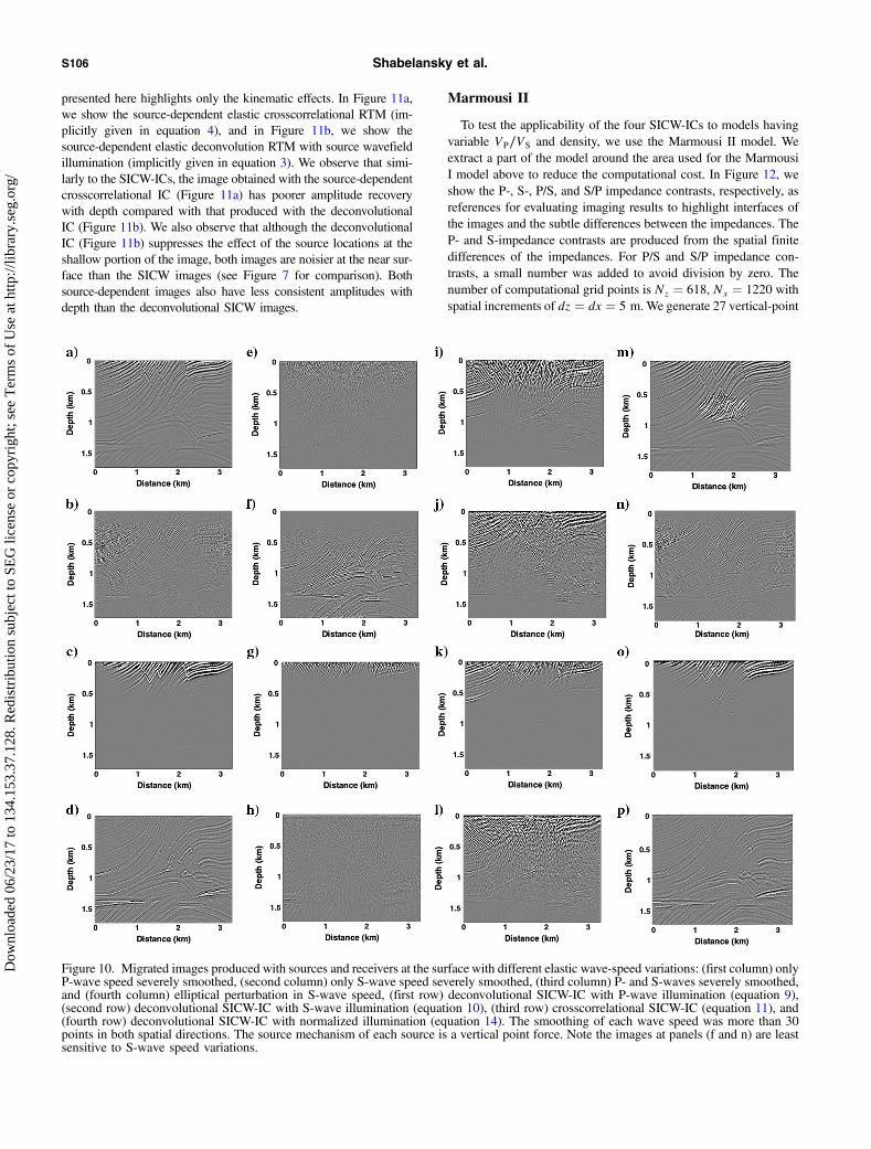
quality of the wave speed models used for imag-ing. For this reason, we have developed a wavespeed estimation approach for use with SICWimaging that allows one to find reliable wavespeed models and thus obtain improved images(Shabelansky et al., 2015b). To highlight the sen-sitivity of SICW-ICs to wave speed variations,we present two sets of imaging results; first withseverely smoothed wave speed models and sec-ond with a smooth elliptical inclusion at thecenter of the S-wave speed model. The smooth-ing is over 30 points in both spatial directions inboth sets. In Figure 10a–10d, we show SICWimages with smoothed P-wave speed and correctS-wave speed and density, in which we observethat the smoothed P-wave speed has minor effecton all SICW-ICs. In Figure 10e–10h, the S-wavespeed is smoothed and the P-wave speedand density are correct. Now, we observe a sig-nificant image degradation obtained with thecrosscorrelation, deconvolution with P-wave il-lumination and with both wave illuminationsSICW-ICs. However, the SICW image obtainedwith S-wave illumination (Figure 10f) interest-ingly is insensitive to S-wave variation. In Fig-ure 10i–10l, we show the images that areobtained with P- and S-wave speeds smoothed.We observe that because the VP∕VS ratio is pre-served the image degradation is less severe thanwhen only one wave speed is smoothed; how-ever, the noise level is higher than with othercases. In Figure 10m–10p, we show the SICW

images obtained with the correct P-wave speed and S-wave speed,which consisted of the correct S-wave speed with an elliptical per-turbation at the center of the model. The reason for inserting theelliptical inclusion into the S-wave speed model stems from the ob-servations of Figure 10e–10h in which we observed that SICP im-ages have strong sensitivity to the S-wave speed variations. Weobserve that the effect of the elliptical inclusion is very pronouncedin the deconvolution SICW image with P-wave illumination (Fig-ure 10m) and in the crosscorrelation SICW image (Figure 10o); weobserve strong amplitude amplification at the area of the S-wavespeed inclusion. In the deconvolution SICW image with both illu-minations (Figure 10p), we observe that the amplitudes are attenu-ated but the image is clear, whereas the SICW image with S-waveillumination (Figure 10n) is insensitive to the inclusion in the S-wave speed model. The insensitivity to S-wave speed is similarto the observation made for Figure 10f.To show a comparison between the SICW-ICs and the source-

dependent ICs, we calculate elastic PP RTM images with crosscor-relation and deconvolution ICs (i.e., we replace the back-propagatingS-wavefield in equations 9 and 11 with the forward-propagatingP-wavefield, respectively). We use the same number of surfacesources, receiver geometry, and the same wave speeds as those cal-culated above in Figure 7. We apply a mute to remove the direct arriv-als in the data. Because the source-dependent RTM produces imagesof reflections of the subsurface and the SICW-ICs produce imagesof the ratios between conversions and reflections, the comparison

Figure 9. Migrated images produced with 130 sources with 24 m horizontal intervals atthe surface and receivers at the surface using (a) deconvolutional SICW-IC with P-waveillumination (equation 9), (b) deconvolutional SICW-IC with S-wave illumination(equation 10), (c) crosscorrelational SICW-IC (equation 11), and (d) deconvolutionalSICW-IC with normalized illumination (equation 14). The images are less noisy thanthose in Figure 7. Although the amplitude balancing of the crosscorrelation SICW imagewas changed due to the increased number of sources, the amplitude balancing of thedeconvolutional SICW images remained the same as in those with a reduced number ofsources (Figure 7a, 7b, and 7d).

Source-independent CW imaging conditions S105

Dow

nloa

ded

06/2

3/17

to 1

34.1

53.3

7.12

8. R

edis

trib

utio

n su

bjec

t to

SEG

lice

nse

or c

opyr

ight

; see

Ter

ms

of U

se a

t http

://lib

rary

.seg

.org

/

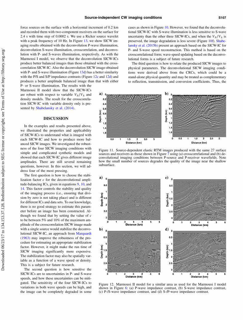
presented here highlights only the kinematic effects. In Figure 11a,we show the source-dependent elastic crosscorrelational RTM (im-plicitly given in equation 4), and in Figure 11b, we show thesource-dependent elastic deconvolution RTM with source wavefieldillumination (implicitly given in equation 3). We observe that simi-larly to the SICW-ICs, the image obtained with the source-dependentcrosscorrelational IC (Figure 11a) has poorer amplitude recoverywith depth compared with that produced with the deconvolutionalIC (Figure 11b). We also observe that although the deconvolutionalIC (Figure 11b) suppresses the effect of the source locations at theshallow portion of the image, both images are noisier at the near sur-face than the SICW images (see Figure 7 for comparison). Bothsource-dependent images also have less consistent amplitudes withdepth than the deconvolutional SICW images.

Marmousi II

To test the applicability of the four SICW-ICs to models havingvariable VP∕VS and density, we use the Marmousi II model. Weextract a part of the model around the area used for the MarmousiI model above to reduce the computational cost. In Figure 12, weshow the P-, S-, P/S, and S/P impedance contrasts, respectively, asreferences for evaluating imaging results to highlight interfaces ofthe images and the subtle differences between the impedances. TheP- and S-impedance contrasts are produced from the spatial finitedifferences of the impedances. For P/S and S/P impedance con-trasts, a small number was added to avoid division by zero. Thenumber of computational grid points is Nz ¼ 618, Nx ¼ 1220 withspatial increments of dz ¼ dx ¼ 5 m. We generate 27 vertical-point

Figure 10. Migrated images produced with sources and receivers at the surface with different elastic wave-speed variations: (first column) onlyP-wave speed severely smoothed, (second column) only S-wave speed severely smoothed, (third column) P- and S-waves severely smoothed,and (fourth column) elliptical perturbation in S-wave speed, (first row) deconvolutional SICW-IC with P-wave illumination (equation 9),(second row) deconvolutional SICW-IC with S-wave illumination (equation 10), (third row) crosscorrelational SICW-IC (equation 11), and(fourth row) deconvolutional SICW-IC with normalized illumination (equation 14). The smoothing of each wave speed was more than 30points in both spatial directions. The source mechanism of each source is a vertical point force. Note the images at panels (f and n) are leastsensitive to S-wave speed variations.

S106 Shabelansky et al.

Dow

nloa

ded

06/2

3/17

to 1

34.1

53.3

7.12

8. R

edis

trib

utio

n su

bjec

t to

SEG

lice

nse

or c

opyr

ight

; see

Ter

ms

of U

se a

t http

://lib

rary

.seg

.org

/

force sources on the surface with a horizontal increment of 0.2 kmand recorded them with two-component receivers on the surface for2.4 s with time step of 0.0002 s. We use a Ricker source waveletwith a peak frequency of 10 Hz. In Figure 13, we show SICW im-aging results obtained with the deconvolution P-wave illumination,deconvolution S-wave illumination, crosscorrelation, and deconvo-lution with P- and S-waves illumination, respectively. As with theMarmousi I model, we observe that the deconvolution SICW-ICsproduce better balanced images than those obtained with the cross-correlation SICW-IC. Also the deconvolution SICW image obtainedwith P- and S-wave illumination (Figure 13d) has a better similaritywith the P/S and S/P impedance contrasts (Figure 12c and 12d) andproduces a better amplitude balanced image than that with eitherP- or S-wave illumination. The results with theMarmousi II model show that the SICW-ICsare robust with respect to variable VP∕VS anddensity models. The result for the crosscorrela-tion SICW-IC with variable density only is pre-sented by Shabelansky et al. (2014).

DISCUSSION

In the examples and results presented above,we illustrated the properties and applicabilityof SICW-ICs to understand what is imaged witheach SICW-IC and how to produce more bal-anced SICW images. We investigated the robust-ness of the four SICW imaging conditions withsimple and complicated synthetic models andshowed that each SICW-IC gives different imageamplitudes. There are still several remainingquestions, however. In this section, we will ad-dress four of the most pressing.The first question is how to choose the stabi-

lization factor ϵ for the deconvolutional ampli-tude-balancing ICs, given in equations 9, 10, and14. This factor controls the stability and qualityof the imaging process (i.e., ensuring that divi-sion by zero is not taking place) and is differentfor different ICs and data sets. To our knowledge,there is no good strategy to estimate this param-eter before an image has been constructed. Al-though we found that by setting the value of ϵto be between 5% and 10% of the maximum am-plitude of the crosscorrelation SICW image madewith a single source would stabilize the deconvo-lutional SICW-IC, an approach from Marquardt(1963) may improve the robustness of the pro-cedure for estimating an appropriate stabilizationfactor. However, it might make the run time ofSICW imaging significantly more expensive.The stabilization factor may also be spatially var-iable as a function of a wave speed or density.This is a subject for future research.The second question is how sensitive the

SICW-ICs are to uncertainties in P- and S-wavespeeds, and how these uncertainties can be miti-gated. The sensitivity of the four SICW-ICs tovariations in both wave speeds can be high, andthe image can be completely degraded in some

cases as shown in Figure 10. However, we found that the deconvolu-tional SICW-IC with S-wave illumination is less sensitive to S-waveuncertainty than the other three SICW-ICs, and when the VP∕VS ispreserved, the image degradation is less severe (Figure 10f). Shabe-lansky et al. (2015b) present an approach based on the SICW-IC forP- and S-wave speed reconstruction. This method is based on thecrosscorrelational form; wave-speed updating based on the deconvo-lutional forms is a subject of future research.The third question is how to relate the produced SICW images to

physical parameters. The deconvolutional SICW imaging condi-tions were derived above from the CRCs, which could be astand-alone physical quantity and may be treated as complementaryto reflection, transmission, and conversion coefficients. Thus, the

Figure 11. Source-dependent elastic RTM images produced with the same 27 surfacesources and receivers as those shown in Figure 7 using (a) crosscorrelational and (b) de-convolutional imaging conditions between P-source and P-receiver wavefields. Notehow the small number of sources degrades the quality of the image near the shallowsubsurface.

Figure 12. Marmousi II model for a similar area as used for the Marmousi I modelshown in Figure 6: (a) P-wave impedance contrast, (b) S-wave impedance contrast,(c) P-/S-wave impedance contrast, and (d) S-/P-wave impedance contrast.

Source-independent CW imaging conditions S107

Dow

nloa

ded

06/2

3/17

to 1

34.1

53.3

7.12

8. R

edis

trib

utio

n su

bjec

t to

SEG

lice

nse

or c

opyr

ight

; see

Ter

ms

of U

se a

t http

://lib

rary

.seg

.org

/

images could be associated by inversion with the CRCs. In particu-lar, the CRCs may be of great interest in studies of amplitude varia-tion with offset/angle/azimuth because they define the ratio of theconverted and pure seismic waves and how their energy is parti-tioned after passing through an impedance contrast.The fourth question is how to apply SICW imaging to an aniso-

tropic medium using the four imaging conditions. The success ofSICW imaging in an anisotropic medium depends on the abilityto separate the propagating waves into quasi P- and S-waves. ForVTI media, many studies show different techniques for wave sep-aration (Dellinger and Etgen, 1990; Yan and Sava, 2009; Yan,2010; Zhang and McMechan, 2010; Cheng and Fomel, 2014).However, they are significantly more computationally expensivethan that shown in Appendix A for the isotropic case. For a moregeneral anisotropy, even further research is required, particularlyin 3D.Our approach relies on wavefield separation using the method

described in Appendix A, and it does not require knowledge of thenormal vector from subsurface reflectors as in Duan and Sava(2015), an estimation of the wavefield vector propagation directionsas in Gong et al. (2016), or an estimation of the Poynting vectors asin Wang and McMechan (2015). The general observations and dis-cussions drawn throughout the text in 2D are expected to be similarin 3D. The application of the 3D crosscorrelational SICW-IC tofield data can be found in Shabelansky (2015, chapter 5). We haveintroduced a novel approach for source-independent seismic imag-ing and illustrated it with a limited number of numerical examplesthat are meant to highlight the differences among the proposed

imaging conditions. We hope that others will explore more numeri-cal examples to evaluate the SICW-ICs and apply them to field data.

CONCLUSION

We have presented crosscorrelational and deconvolutional formsof an SICW-IC, and we investigated their relationship with reflection,transmission, and conversion coefficients through a newly introducedconcept of CRCs. We illustrated the properties of the CRCs and dem-onstrated their use through deconvolutional imaging conditions withdifferent types of illumination compensation. We tested the imagingconditions with a two half-space model, and the synthetic MarmousiI and II models. We also showed the sensitivity of the SICW-ICs to P-and S-wave speed perturbations and presented a comparison betweenthe SICW-ICs and the source-dependent elastic RTM. The resultsshow advantages when appropriate illumination compensation inSICW-IC is applied and that SICW-IC with S-wave illumination isless sensitive to S-wave speed perturbation than the other SICW-ICs.The introduced SICW-ICs present attractive alternatives to elasticsource-dependent RTM imaging.

ACKNOWLEDGMENTS

We thank ConocoPhillips and the Earth Resources Laboratory(ERL) founding members consortium at MIT for funding this work.Partial support for this work was provided by the Department ofEnergy, Lawrence Berkeley National Laboratory, subcontract#6927716, entitled, “Advanced 3D Geophysical Imaging Technolo-

gies for Geothermal Resource Characterization.”We acknowledge S. K. Bakku, A. Tryggvason,and O. Gudmundsson for their helpful discus-sions. We also acknowledge the associate and as-sistant editors and six anonymous reviewerswhose comments helped significantly to improvethe manuscript.

APPENDIX A

P-S WAVEFIELD SEPARATIONUSING ACCELERATION

DECOMPOSITION

The images produced with P- and S-waves de-pend on the P-S wavefield separation. Separationusing the Helmholtz decomposition (i.e., applyingonly the divergence and curl operators) producesimages with inconsistent amplitude and phase thatthus require correction before or after the con-struction of the images (Sun et al., 2004, 2011;Shang et al., 2012; Shabelansky et al., 2013b).Separation using the vector wavefield decomposi-tion is computationally more expensive, but it pro-duces images with consistent amplitude polarity.The vector wavefield separation is derived from

the isotropic elastic-wave equation for a smoothmedium (Aki and Richards, 2002, p. 64) as

u ¼ α2∇∇ · u − β2∇ × ∇ × u; (A-1)

where uðx; tÞ and uðx; tÞ are the displacement andacceleration vector wavefields, αðxÞ and βðxÞ are

Figure 13. Marmousi II: migrated images produced with 27 sources with 0.2 km hori-zontal interval at the surface and receivers at the surface using (a) deconvolutionalSICW-IC with P-wave illumination (equation 9), (b) deconvolutional SICW-IC withS-wave illumination (equation 10), (c) crosscorrelational SICW-IC (equation 11), and(d) deconvolutional SICW-IC with normalized illumination (equation 14). The sourcemechanism of each source is a vertical point force. Despite a certain level of noise in allimages, the image amplitudes in panel (d) are the most balanced.

S108 Shabelansky et al.

Dow

nloa

ded

06/2

3/17

to 1

34.1

53.3

7.12

8. R

edis

trib

utio

n su

bjec

t to

SEG

lice

nse

or c

opyr

ight

; see

Ter

ms

of U

se a

t http

://lib

rary

.seg

.org

/

the P- and S-wave speeds, and ∇, ∇ ·, and ∇× are the gradient, di-vergence, and curl operators, respectively. Because the accelerationwavefield is decomposed into α2∇∇ · u and −β2∇ × ∇ × u, we de-fine u ¼ uP þ uS with

uPðx; tÞ ¼ α2ðxÞ∇∇ · uðx; tÞ;uSðx; tÞ ¼ −β2ðxÞ∇ × ∇ × uðx; tÞ; (A-2)

where uP and uS are the P- and S-components of acceleration. Be-cause αðxÞ and βðxÞ are in general smooth for imaging, we removethe effect of the P- and S-wave speeds on wavefield separation andobtain

uP ¼ ∇∇ · u; uS ¼ −∇ × ∇ × u; (A-3)

where uPðx; tÞ and uSðx; tÞ are the P- and S-vector components of theseparated displacement vector wavefield uðx; tÞ with the velocitiesremoved in equation A-2. By removing the (squared) wave speedsfrom equation A-2, we obtain units of inverse displacement (i.e.,1∕m) in equation A-3. Note that the operators ∇∇ · and −∇ × ∇in equation A-2 can be similarly applied to the particle velocity oracceleration wavefields. Then the units of the separated wavefieldswill be proportional to 1∕ms or 1∕ms2, respectively. The wave speedremoval procedure reduces strong dependence of imaging on wavespeeds and thus produces more balanced images. However, for wavespeed optimization analysis, care needs to be taken because this pro-cedure affects to construction of the gradient for the optimization. Formore details, see Shabelansky et al. (2015b) and Shabelansky (2015,appendix B).

REFERENCES

Aki, K., and P. G. Richards, 2002, Quantitative seismology, theory andmethods, 2nd ed.: University Science Books.

Baysal, E., D. D. Kosloff, and J. W. C. Sherwood, 1983, Reverse time mi-gration: Geophysics, 48, 1514–1524, doi: 10.1190/1.1441434.

Bleistein, N., 1987, On the imaging of reflectors in the earth: Geophysics,52, 931–942, doi: 10.1190/1.1442363.

Brytic, V., M. V. de Hoop, and R. D. van der Hilst, 2012, Elastic-wave in-verse scattering based on reverse time migration with active and passivesource reflection data, in G. Uhlmann, ed., Inverse problems and appli-cations: Inside out II: MSRI Publications 60, 411.

Chang, W.-F., and G. A. McMechan, 1994, 3-D elastic prestack, reverse-time depth migration: Geophysics, 59, 597–609, doi: 10.1190/1.1443620.

Chattopadhyay, S., and G. A. McMechan, 2008, Imaging conditions for pre-stack reverse time migration: Geophysics, 73, no. 3, S81–S89, doi: 10.1190/1.2903822.

Cheng, J., and S. Fomel, 2014, Fast algorithms for elastic-wave-mode sep-aration and vector decomposition using low-rank approximation foranisotropic media: Geophysics, 79, no. 4, C97–C110, doi: 10.1190/geo2014-0032.1.

Claerbout, J. F., 1971, Toward a unified theory of reflector mapping: Geo-physics, 36, 467–481, doi: 10.1190/1.1440185.

Claerbout, J. F., 1985, Imaging the earth’s interior: Blackwell ScientificInc.

Dellinger, J., and J. Etgen, 1990, Wave-field separation in two-dimensionalanisotropic media: Geophysics, 55, 914–919, doi: 10.1190/1.1442906.

Duan, Y., and P. Sava, 2015, Scalar imaging condition for elastic reversetime migration: Geophysics, 80, no. 4, S127–S136, doi: 10.1190/geo2014-0453.1.

Gong, T., B. D. Nguyen, and G. A. McMechan, 2016, Polarized wavefieldmagnitudes with optical flow for elastic angle-domain common-imagegathers: Geophysics, 81, no. 4, S239–S251, doi: 10.1190/geo2015-0518.1.

Kaelin, B., and A. Guitton, 2006, Imaging condition for reverse time migra-tion: 76th Annual International Meeting, SEG, Expanded Abstracts,2594–2598.

Marquardt, D. W., 1963, An algorithm for least-squares estimation of non-linear parameters: Journal of the Society for Industrial & Applied Math-ematics, 11, 431–441, doi: 10.1137/0111030.

Nihei, K. T., S. Nakagawa, and L. R. Myer, 2001, Fracture imaging withconverted elastic waves: Lawrence Berkeley National Laboratory,LBNL–50789.

Popovici, A. M., 1996, Prestack migration by split-step DSR: Geophysics,61, 1412–1416, doi: 10.1190/1.1444065.

Schneider, W. A., 1978, Integral formulation for migration in two and threedimensions: Geophysics, 43, 49–76, doi: 10.1190/1.1440828.

Schleicher, J., J. C. Costa, and A. Novais, 2008, A comparison of imagingconditions for wave-equation shot-profile migration: Geophysics, 73,no. 6, S219–S227, doi: 10.1190/1.2976776.

Shabelansky, A. H., 2015, Theory and application of source independent fullwavefield elastic converted phase seismic imaging and velocity analysis:Ph.D. thesis, Massachusetts Institute of Technology.

Shabelansky, A. H., M. C. Fehler, and A. E. Malcolm, 2013a, Converted-phase seismic imaging of the Hengill region, southwest Iceland: Presentedat the AGU Fall Meeting Abstracts, A2461.

Shabelansky, A. H., A. Malcolm, and M. Fehler, 2015a, Converted-phaseseismic imaging-amplitude-balancing source-independent imaging condi-tions: 77th Annual International Conference and Exhibition, EAGE,Extended Abstracts, doi: 10.3997/2214-4609.201412937.

Shabelansky, A. H., A. Malcolm, M. Fehler, and W. L. Rodi, 2014,Migration-based seismic trace interpolation of sparse converted phasemicro-seismic data: 84th Annual International Meeting, SEG, ExpandedAbstracts, 3642–3647.

Shabelansky, A. H., A. Malcolm, M. Fehler, X. Shang, and W. L. Rodi,2013b, Converted phase elastic migration velocity analysis: 83rd AnnualInternational Meeting, SEG, Expanded Abstracts, 4732–4737.

Shabelansky, A. H., A. Malcolm, M. C. Fehler, X. Shang, and W. L. Rodi,2015b, Source-independent full wavefield converted-phase elastic migra-tion velocity analysis: Geophysical Journal International, 200, 952–966,doi: 10.1093/gji/ggu450.

Shang, X., M. de Hoop, and R. van der Hilst, 2012, Beyond receiver func-tions: Passive source reverse time migration and inverse scattering ofconverted waves: Geophysical Research Letters, 39, 1–7, doi: 10.1029/2012GL052289.

Stoffa, P. L., J. T. Fokkema, R. M. de Luna Freire, andW. P. Kessinger, 1990,Split-step Fourier migration: Geophysics, 55, 410–421, doi: 10.1190/1.1442850.

Sun, R., G. A. McMechan, and H.-H. Chuang, 2011, Amplitude balancing inseparating P- and S-waves in 2D and 3D elastic seismic data: Geophysics,76, no. 3, S103–S113, doi: 10.1190/1.3555529.

Sun, R., G. A. McMechan, H.-H. Hsiao, and J. Chow, 2004, SeparatingP-and S-waves in prestack 3D elastic seismograms using divergenceand curl: Geophysics, 69, 286–297, doi: 10.1190/1.1649396.

Valenciano, A., and B. Biondi, 2003, 2-D deconvolution imaging conditionfor shot-profile migration: 73rd Annual International Meeting, SEG,Expanded Abstracts, 1059–1062.

Wang, W., and G. A. McMechan, 2015, Vector-based elastic reverse timemigration: Geophysics, 80, no. 6, S245–S258, doi: 10.1190/geo2014-0620.1.

Xiao, X., and W. S. Leaney, 2010, Local vertical seismic profiling (VSP)elastic reverse-time migration and migration resolution: Salt-flank imag-ing with transmitted P-to-S waves: Geophysics, 75, no. 2, S35–S49, doi:10.1190/1.3309460.

Yan, J., 2010, Wave-mode separation for elastic imaging in transverselyisotropic media: Ph.D. thesis, Colorado School of Mines.

Yan, J., and P. Sava, 2009, Elastic wave-mode separation for VTImedia: Geophysics, 74, no. 5, WB19–WB32, doi: 10.1190/1.3184014.

Youn, O. K., and H.-W. Zhou, 2001, Depth imaging with multiples:Geophysics, 66, 246–255, doi: 10.1190/1.1444901.

Zhang, Q., and G. A. McMechan, 2010, 2D and 3D elastic wavefield vectordecomposition in the wavenumber domain for VTI media: Geophysics,75, no. 3, D13–D26, doi: 10.1190/1.3431045.

Zhang, Y., and J. Sun, 2008, Practical issues of reverse time migration-true-amplitude gathers, noise removal and harmonic-source encoding:70th Annual International Conference and Exhibition, EAGE, ExtendedAbstracts, doi: 10.3997/2214-4609.20147708.

Source-independent CW imaging conditions S109

Dow

nloa

ded

06/2

3/17

to 1

34.1

53.3

7.12

8. R

edis

trib

utio

n su

bjec

t to

SEG

lice

nse

or c

opyr

ight

; see

Ter

ms

of U

se a

t http

://lib

rary

.seg

.org

/