seismic characterization of naturally fractured reservoirs ... · pdf filegeophysical...

$: Seismic characterization of naturally fractured reservoirs ... · PDF fileGeophysical Prospecting doi: 10.1111/1365-2478.12011 Seismic characterization of naturally fractured reservoirs$
Geophysical Prospecting doi: 10.1111/1365-2478.12011

Seismic characterization of naturally fractured reservoirs usingamplitude versus offset and azimuth analysis

Mehdi E. Far1∗, Colin M. Sayers1,2, Leon Thomsen1,3, De-hua Han1 and

John P. Castagna1

1University of Houston2Schlumberger and 3Delta Geophysics

Received March 2012, revision accepted September 2012

ABSTRACTP-wave seismic reflection data, with variable offset and azimuth, acquired over afractured reservoir can theoretically be inverted for the effective compliance of thefractures. The total effective compliance of a fractured rock, which is described usingsecond- and fourth-rank fracture tensors, can be represented as background compli-ance plus additional compliance due to fractures. Assuming monoclinic or orthotropicsymmetry (which take into account layering and multiple fracture sets), the compo-nents of the effective second- and fourth-rank fracture compliance tensors can be usedas attributes related to the characteristics of the fractured medium. Synthetic tests in-dicate that using a priori knowledge of the properties of the unfractured medium, theinversion can be effective on noisy data, with S/N on the order of 2. Monte Carlosimulation was used to test the effect of uncertainties in the a priori information aboutelastic properties of unfractured rock. Two cases were considered with Wide Azimuth(WAZ) and Narrow Azimuth (NAZ) reflection data and assuming that the fractureshave rotationally invariant shear compliance. The relative errors in determination ofthe components of the fourth-rank tensor are substantially larger compared to thesecond-rank tensor, under the same assumptions.

Elastic properties of background media, consisting in horizontal layers withoutfractures, do not cause azimuthal changes in the reflection coefficient variation withoffset. Thus, due to the different nature of these properties compared to fracturetensor components (which cause azimuthal anomalies), simultaneous inversion forbackground isotropic properties and fracture tensor components requires additionalconstraints.

Singular value decomposition (SVD) and resolution matrix analysis can be used topredict fracture inversion efficacy before acquiring data. Therefore, they can be usedto determine the optimal seismic survey design for inversion of fracture parameters.However, results of synthetic inversion in some cases are not consistent with resolu-tion matrix results and resolution matrix results are reliable only after one can see aconsistent and robust behaviour in inversion of synthetics with different noise levels.

Key words: Fractures, AVOA, Reflection coefficient, Inversion, Singular value de-composition.

∗Email: [email protected]

C© 2013 European Association of Geoscientists & Engineers 1

2 Mehdi E. Far et al.

INTRODUCTIO N

Natural and induced fractures in reservoirs play an impor-tant role in determining fluid flow during production andknowledge of the orientation and density of fractures is usefulto optimize production from fractured reservoirs (e.g., Reiss1980; Nelson 1985). Areas of high-fracture density may rep-resent zones of high permeability, therefore locating wells inthese areas may be important. Fractures usually show pre-ferred orientations and this may result in significant perme-ability anisotropy in the reservoir. It is important for optimumdrainage that producers should be more closely spaced alongthe direction of minimum permeability than along the direc-tion of maximum permeability and the azimuthal orientationof deviated wells should be chosen to maximize productiontaking into account the orientation of fractures (Sayers 2009).

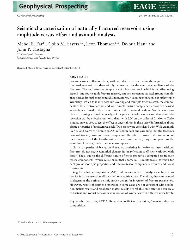
Seismic anisotropy is defined as the dependence of seismicvelocity upon angle. Seismic velocity anisotropy can be causedby different factors, such as rock fabric, grain-scale microc-racks, rock layering and aligned fractures at all scales, pro-vided that the characteristic dimensions of these features aresmall relative to the seismic wavelength (Worthington 2008).As a result, P-waves propagating parallel to fractures willbe faster than those propagating perpendicular to fractures(Fig. 1).

The use of seismic waves to determine the orientation offractures has received much attention. For example, Lynn

Figure 1 Reflection from a fractured layer with a single set of parallelvertical fractures for acquisition parallel and perpendicular to thefractures

et al. (1994) used the azimuthal variation in the reflectionamplitude of seismic P-waves to characterize fractured reser-voirs (see also Eftekharifar and Sayers 2011a, b). Reflectionamplitudes have advantages over seismic velocities for char-acterizing fractured reservoirs because they have higher ver-tical resolution. However, the interpretation of variations inreflection amplitude requires a model of sufficient complex-ity to allow the measured change in reflection amplitude tobe inverted correctly for the characteristics of the fracturedreservoir (Sayers 2009).

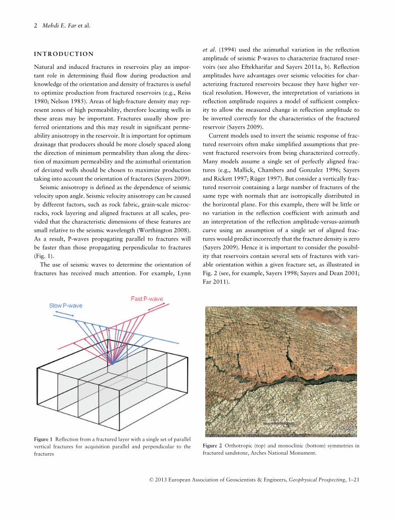
Current models used to invert the seismic response of frac-tured reservoirs often make simplified assumptions that pre-vent fractured reservoirs from being characterized correctly.Many models assume a single set of perfectly aligned frac-tures (e.g., Mallick, Chambers and Gonzalez 1996; Sayersand Rickett 1997; Ruger 1997). But consider a vertically frac-tured reservoir containing a large number of fractures of thesame type with normals that are isotropically distributed inthe horizontal plane. For this example, there will be little orno variation in the reflection coefficient with azimuth andan interpretation of the reflection amplitude-versus-azimuthcurve using an assumption of a single set of aligned frac-tures would predict incorrectly that the fracture density is zero(Sayers 2009). Hence it is important to consider the possibil-ity that reservoirs contain several sets of fractures with vari-able orientation within a given fracture set, as illustrated inFig. 2 (see, for example, Sayers 1998; Sayers and Dean 2001;Far 2011).

Figure 2 Orthotropic (top) and monoclinic (bottom) symmetries infractured sandstone, Arches National Monument.

C© 2013 European Association of Geoscientists & Engineers, Geophysical Prospecting, 1–21

Seismic characterization of naturally fractured reservoirs 3

The simple model of Horizontally Transverse Isotropic(HTI) symmetry, which assumes one set of aligned verticalfractures (with rotationally invariant shear compliance) em-bedded in an otherwise isotropic background is misleadingfor another reason. In the HTI model, horizontal layering ofsediments, leading to a variation of velocity with polar angle,is ignored. Hence HTI is not a suitable model in sedimentarybasins, where layering is ubiquitous and no fractures can bepresumed to lie within an ‘otherwise isotropic background’,although it may be useful in the igneous crust, for which itwas originally proposed (e.g., Crampin 1984).

In this work, the linear slip theory (see below) is used todescribe the relation between stress and fracture strain, asexpressed by the specific compliances of the fractures. Thistheory describes fractures using normal and tangential spe-cific compliances of fractures, without detailed assumptionsconcerning the microgeometry of the fractures. It is assumedthat the specific shear compliance of fractures is rotationallyinvariant around the normal to the fractures (this work willbe generalized in a future paper to the case of rotationally-dependent shear compliance, enabling the analysis of joints,which are much longer horizontally than vertically.) Thom-sen (1995) showed the effect of frequency and squirt flowon elastic properties of fractured rocks, including their in-teraction with equant (non-fracture) porosity. At higher fre-quencies, fluid-filled fractures tend to be stiffer than at lowerfrequencies. Based on data from several authors, Worthing-ton (2008) showed that fracture specific compliances are di-rectly related to fracture dimension. The theory developed byKachanov (1980) and Sayers and Kachanov (1991, 1995) isused for effective medium modelling of media with fractureshaving rotationally invariant shear compliance. Kachanov(1980) applied this approach to modelling permeabilityalso.

Fracture characterization using surface seismic data de-mands wide azimuth surveys. Due to the high cost of wideazimuth seismic data acquisition, the determination of az-imuth/offset characteristics in such data, for the task of frac-ture modelling, becomes very important, as does optimizationof the acquisition for revealing such characteristics. This op-timization will be demonstrated using Singular Value Decom-position (SVD) and inversion of synthetic Amplitude VersusOffset and Azimuth (AVOA) data. Synthetic AVOA data fordifferently oriented vertical fractures are analysed, in order toidentify which parameter combinations are well-resolved byvarious experimental geometries. Synthetic reflectivity dataare also used to invert for the components of the additionaleffective fracture compliance tensor. Inversion results are in

general consistent with resolution matrix results with differ-ent noise levels, proving the usefulness of SVD for this inverseproblem.

LINEAR S LIP CONDITION

The small vector difference (across a fracture) in the displace-ment field u is assumed to depend linearly on the tractionvector t. This dependence may be assumed to be real andfrequency independent, corresponding to an elastic springcondition, or it may be assumed to be complex and fre-quency dependent (Jones and Whittier 1967; Schoenberg1980).

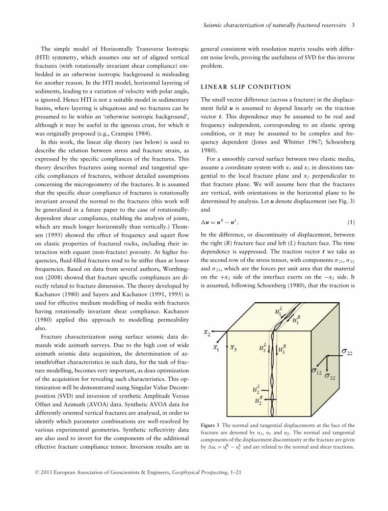
For a smoothly curved surface between two elastic media,assume a coordinate system with x1 and x3 in directions tan-gential to the local fracture plane and x2 perpendicular tothat fracture plane. We will assume here that the fracturesare vertical, with orientations in the horizontal plane to bedetermined by analysis. Let u denote displacement (see Fig. 3)and

�u = uR − uL, (1)

be the difference, or discontinuity of displacement, betweenthe right (R) fracture face and left (L) fracture face. The timedependency is suppressed. The traction vector t we take asthe second row of the stress tensor, with components σ 21, σ 22

and σ 23, which are the forces per unit area that the materialon the +x2 side of the interface exerts on the −x2 side. Itis assumed, following Schoenberg (1980), that the traction is

Figure 3 The normal and tangential displacements at the face of thefracture are denoted by u3, u1 and u2. The normal and tangentialcomponents of the displacement discontinuity at the fracture are givenby �ui = uR

i − uLi and are related to the normal and shear tractions.



linearly dependent on the displacement slip:

t(�u) ≈ k�u, (2)

where k is the specific stiffness matrix.If the specific stiffness matrix k is required to be invariant

with respect to inversion of x2, it can be shown (Schoenberg1980) that off-diagonal terms k21, k12, k32 and k23, betweenthe normal and tangential directions, must be zero. If there isrotational symmetry for shear compliance around the x2 axis,it can be shown that k13 = k31 = 0, k11 = k33 = kT and k22 =kN (Schoenberg 1980).

It is convenient to characterize compliances instead of stiff-nesses, which are the inverse of a compliance matrix. One canwrite (Kachanov 1980):

�u =

⎡⎢⎢⎣

BT 0 0

0 BN 0

0 0 BT

⎤⎥⎥⎦ t, (3)

where BN = kN−1 and BT = kT

−1 are the normal and tangentialspecific fracture compliances respectively and their dimensionis length/stress. BN gives the displacement discontinuity in thedirection normal to the fracture for a unit normal traction andBT gives the displacement discontinuity parallel to the fractureplane for unit shear traction (see Fig. 3). If there are multiplefractures, then the effective compliances of a given fracturewill be affected by the presence of the other fractures. Theyalso depend on the fluid content and fracture density. In indexnotation, equation (3) is:

�ui = Bi j tj , (4)

with B11 = B33 = BT and B22 = BN. The specific compli-ance tensor B above is written for the case of fractures withrotationally invariant shear compliance, normal to the x2 di-rection; for a fracture with arbitrary orientation, it may bewritten compactly as (Kachanov 1980):

Bi j = BNni n j + BT(δi j − ni n j ). (5)

The boundary conditions shown in equation (4) were firstused by Jones and Whittier (1967) for modelling of wavepropagation through a flexibly bonded interface by allow-ing both slip and separation. The vanishing of either or bothof these specific compliances leads to perfectly bonded in-terface conditions. Real elastic parameters may be general-ized to complex frequency- dependent viscoelastic parameters,therefore linear viscoelastic interfaces can be modelled as well(Schoenberg 1980).

Schoenberg’s linear slip theory was originally developed fora single set of fractures (with rotationally invariant shear com-

pliance) embedded in isotropic host rock and later was ex-tended to several fracture sets (see, for example, Schoenbergand Muir 1989; Schoenberg and Sayers, 1995) and also toanisotropic backgrounds (e.g., Sayers and Kachanov 1991,1995; Helbig 1994; Schoenberg and Sayers 1995).

A R B I T R A R Y V E R T I C A L F R A C T U R E S

In an elastic medium that contains an arbitrary number of setsof fractures with arbitrary orientation distribution, using thedivergence theorem and Hooke’s law, it can be shown (Hill1963; Sayers and Kachanov 1995) that the elastic compliancetensor of the fractured medium can be written in the followingform:

Si jkl = S0i jkl + �Si jkl , (6)

where S0 is the compliance matrix of the medium (includingthe effects of pores, cracks and stress except for those fracturesexplicitly included in �S).

Following Nichols, Muir and Schoenberg (1989), the addi-tional (effective) compliance matrix �S, for n sets of alignedfractures can be written as:

�S =n∑

q=1

�Sq, (7)

where �Sq is the additional effective compliance matrix of theqth set of aligned fractures in the presence of the other fracturesets. Implicitly, each of these effective fracture compliancesdepends upon the rest of the rock, specifically including thepresence, location, size and orientation of the other fracturesand pores (including their intersections, if liquid-filled).

Sayers and Kachanov (1991, 1995) derived the effectiveadditional compliance matrix due to fractures with rotation-ally invariant shear compliance. Using equations (6)–(8), theeffective excess compliance �Sijkl due to the presence of thefractures can be written as:

�Si jkl = 14

(δikα jl + δilα jk + δ jkαil + δ jlαik) + βi jkl . (8)

Here, δij is the Kronecker delta, αij is a second-rank tensor andβ ijkl is a fourth-rank tensor defined by:

αi j = 1V

∑r

B(r )T n(r )

i n(r )j A(r ), (9)

βi jkl = 1V

∑r

(B(r )

N − B(r )T

)n(r )

i n(r )j n(r )

k n(r )l A(r ), (10)

where the sum is over all fractures in volume V. Variable ni(r)

is the ith component of the normal to the rth fracture and A(r)



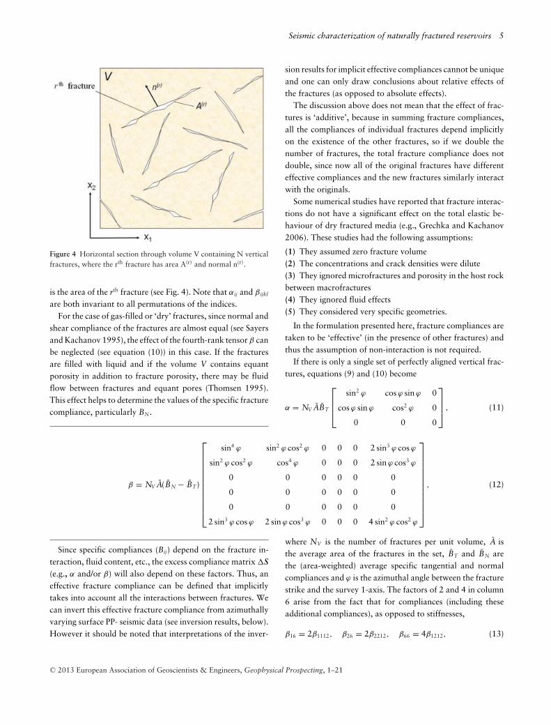
Figure 4 Horizontal section through volume V containing N verticalfractures, where the rth fracture has area A(r) and normal n(r).

is the area of the rth fracture (see Fig. 4). Note that αij and β ijkl

are both invariant to all permutations of the indices.For the case of gas-filled or ‘dry’ fractures, since normal and

shear compliance of the fractures are almost equal (see Sayersand Kachanov 1995), the effect of the fourth-rank tensor β canbe neglected (see equation (10)) in this case. If the fracturesare filled with liquid and if the volume V contains equantporosity in addition to fracture porosity, there may be fluidflow between fractures and equant pores (Thomsen 1995).This effect helps to determine the values of the specific fracturecompliance, particularly BN.

Since specific compliances (Bij) depend on the fracture in-teraction, fluid content, etc., the excess compliance matrix �S(e.g., α and/or β) will also depend on these factors. Thus, aneffective fracture compliance can be defined that implicitlytakes into account all the interactions between fractures. Wecan invert this effective fracture compliance from azimuthallyvarying surface PP- seismic data (see inversion results, below).However it should be noted that interpretations of the inver-

sion results for implicit effective compliances cannot be uniqueand one can only draw conclusions about relative effects ofthe fractures (as opposed to absolute effects).

The discussion above does not mean that the effect of frac-tures is ‘additive’, because in summing fracture compliances,all the compliances of individual fractures depend implicitlyon the existence of the other fractures, so if we double thenumber of fractures, the total fracture compliance does notdouble, since now all of the original fractures have differenteffective compliances and the new fractures similarly interactwith the originals.

Some numerical studies have reported that fracture interac-tions do not have a significant effect on the total elastic be-haviour of dry fractured media (e.g., Grechka and Kachanov2006). These studies had the following assumptions:

(1) They assumed zero fracture volume(2) The concentrations and crack densities were dilute(3) They ignored microfractures and porosity in the host rockbetween macrofractures(4) They ignored fluid effects(5) They considered very specific geometries.

In the formulation presented here, fracture compliances aretaken to be ‘effective’ (in the presence of other fractures) andthus the assumption of non-interaction is not required.

If there is only a single set of perfectly aligned vertical frac-tures, equations (9) and (10) become

α = NV ABT

⎡⎢⎢⎣

sin2 ϕ cos ϕ sin ϕ 0

cos ϕ sin ϕ cos2 ϕ 0

0 0 0

⎤⎥⎥⎦ , (11)

β = NV A(BN − BT)

⎡⎢⎢⎢⎢⎢⎢⎢⎢⎢⎢⎢⎣

sin4 ϕ sin2 ϕ cos2 ϕ 0 0 0 2 sin3 ϕ cos ϕ

sin2 ϕ cos2 ϕ cos4 ϕ 0 0 0 2 sin ϕ cos3 ϕ

0 0 0 0 0 0

0 0 0 0 0 0

0 0 0 0 0 0

2 sin3 ϕ cos ϕ 2 sin ϕ cos3 ϕ 0 0 0 4 sin2 ϕ cos2 ϕ

⎤⎥⎥⎥⎥⎥⎥⎥⎥⎥⎥⎥⎦

, (12)

where NV is the number of fractures per unit volume, A isthe average area of the fractures in the set, BT and BN arethe (area-weighted) average specific tangential and normalcompliances and ϕ is the azimuthal angle between the fracturestrike and the survey 1-axis. The factors of 2 and 4 in column6 arise from the fact that for compliances (including theseadditional compliances), as opposed to stiffnesses,

β16 = 2β1112, β26 = 2β2212, β66 = 4β1212, (13)



according to the Voigt two-index notation. It is shown inthe Appendix A that, if the background medium is isotropic,this case yields ‘HTI’ symmetry, which as discussed aboveis not a suitable approximation in sedimentary basins. If thebackground medium is polar anisotropic, this case yields or-thotropic symmetry.

If there are two sets of perfectly aligned vertical fractures,oriented orthogonally, then equations (9) and (10) become:

α = NV1 A1 BT1

⎡⎢⎢⎣

sin2 ϕ1 cos ϕ1 sin ϕ1 0

cos ϕ1 sin ϕ1 cos2 ϕ1 0

0 0 0

⎤⎥⎥⎦

+ NV2 A2 BT2

⎡⎢⎢⎣

cos2 ϕ1 − sin ϕ1 cos ϕ1 0

− sin ϕ1 cos ϕ1 sin2 ϕ1 0

0 0 0

⎤⎥⎥⎦ ,

(14)

β = NV1 A1(BN1 − BT1)

×

⎡⎢⎢⎢⎢⎢⎢⎢⎢⎢⎣

sin4 ϕ1 sin2 ϕ1 cos2 ϕ1 0 0 0 2 sin3 ϕ1 cos ϕ1

sin2 ϕ1 cos2 ϕ1 cos4 ϕ1 0 0 0 2 sin ϕ1 cos3 ϕ1

0 0 0 0 0 0

0 0 0 0 0 0

0 0 0 0 0 0

2 sin3 ϕ1 cos ϕ1 2 sin ϕ1 cos3 ϕ1 0 0 0 4 sin2 ϕ1 cos2 ϕ1

⎤⎥⎥⎥⎥⎥⎥⎥⎥⎥⎦

+ NV2 A2(BN2 − BT2)

×

⎡⎢⎢⎢⎢⎢⎢⎢⎢⎢⎣

cos4 ϕ1 cos2 ϕ1 sin2 ϕ1 0 0 0 −2 cos3 ϕ1 sin ϕ1

cos2 ϕ1 sin2 ϕ1 sin4 ϕ1 0 0 0 −2 cos ϕ1 sin3 ϕ1

0 0 0 0 0 0

0 0 0 0 0 0

0 0 0 0 0 0

−2 cos3 ϕ1 sin ϕ1 −2 cos ϕ1 sin3 ϕ1 0 0 0 4 cos2 ϕ1 sin2 ϕ1

⎤⎥⎥⎥⎥⎥⎥⎥⎥⎥⎦

,

(15)

where ϕ1 is the azimuthal angle between the fracture set withlabel 1 and the survey 1-axis. It is shown in Appendix A thatthis results in orthotropic symmetry.

If the two fracture sets are not orthogonal but are per-fectly aligned (within each set), then equations (14) and (15)become,

α = NV1 A1 BT1

⎡⎢⎢⎣



0 0 0

⎤⎥⎥⎦

+ NV2 A2 BT2

⎡⎢⎢⎣



0 0 0

⎤⎥⎥⎦ ,

(16)

β = NV1 A1(BN1 − BT1)

×

⎡⎢⎢⎢⎢⎢⎢⎢⎢⎢⎣


sin2 ϕ1 cos2 ϕ1 cos4 ϕ1 0 0 0 2 sin ϕ1 cos3 ϕ1

0 0 0 0 0 0

0 0 0 0 0 0

0 0 0 0 0 0


⎤⎥⎥⎥⎥⎥⎥⎥⎥⎥⎦

+ NV2 A2(BN2 − BT2)

×

⎡⎢⎢⎢⎢⎢⎢⎢⎢⎢⎣


0 cos4 ϕ2 0 0 0 2 sin ϕ2 cos3 ϕ2

0 0 0 0 0 0

0 0 0 0 0 0

0 0 0 0 0 0


⎤⎥⎥⎥⎥⎥⎥⎥⎥⎥⎦

,

(17)

where ϕ2 is the azimuthal angle to the fracture set with label2. In each of these special cases, there is a corresponding re-duction in the number of degrees of freedom; in what followswe consider the general case, with 8 degrees of freedom (3elements of α and 5 of β).

If the background medium is isotropic or transverselyisotropic and there are at least two non-orthogonal verticalfracture sets, this leads to monoclinic symmetry of the frac-tured rock, with a stiffness matrix given by:

CMono. =

⎡⎢⎢⎢⎢⎢⎢⎢⎢⎢⎢⎢⎢⎢⎣

C11 C12 C13 0 0 C16

C12 C22 C23 0 0 C26

C13 C23 C33 0 0 C36

0 0 0 C44 C45 0

0 0 0 C45 C55 0

C16 C26 C36 0 0 C66

⎤⎥⎥⎥⎥⎥⎥⎥⎥⎥⎥⎥⎥⎥⎦

, (18)

and a compliance matrix of similar form. We can choose axesx1 and x2 such that C45 = 0; this is the principal coordinate sys-tem. In the present context, where the azimuthal anisotropy iscaused by fractures, this choice of coordinate system diagonal-izes αij (Sayers 1998). Therefore, for a vertically propagatingshear wave, the fast and slow polarization directions will be inthe direction of x1 and x2, which coincide with the principaldirections of αij. For a coordinate system not so aligned, theazimuth ϕS1 of the fast vertical shear wave is given by (Sayers1998):



tan(2ϕS1) = 2α12/(α11 − α22). (19)

This angle may be determined in the field, from the polar-ization of the fast shear wave measured in a well or a verticalseismic profile.

An important issue in fracture modelling for seismic ex-ploration is the choice of coordinate system. In real worldproblems, the azimuthal orientation of fractures is usually un-known. Therefore, the problem of characterizing fracturedreservoirs should be analysed without assuming that theseorientations are known. Taking into account the generalityof coordinate systems, the fracture compliance matrix in thiswork can be categorized into 6 classes by considering the fol-lowing criteria:

(1) Isotropic or polar anisotropic (‘VTI’) background(2) One or more sets of fractures, not necessarily perfectlyaligned within any set(3) Alignment or non-alignment of fractures with the coordi-nate axes.

The effective compliance tensor Sijkl can be calculated usingequation (6). Since seismologists require the stiffness tensorinstead, when the fracture compliance �S is small, one can di-rectly calculate the stiffness matrix using the additional com-pliance due to fractures, �Sijkl and the background stiffnessmatrix C0 (e.g., Sayers 2009):

C = C0 − C0 �S C0. (20)

We will assume a polar anisotropic background. Anisotropic background is a special case of this. In order tomaintain generality, each fracture is characterized by its ex-cess compliance, not by its shape or size, which we do notspecify here.

The additional compliance, �S, due to two or more setsof aligned vertical fractures, not aligned with the coordinate

system, has the form:

�S =

⎡⎢⎢⎢⎢⎢⎢⎢⎢⎢⎢⎢⎣

α11 + β1111 β1122 0 0 0 α12 + 2β1112

β1122 α22 + β2222 0 0 0 α12 + 2β1222

0 0 0 0 0 0

0 0 0 α22 α12 0

0 0 0 α12 α11 0

α12 + 2β1112 α12 + 2β1222 0 0 0 α11 + α22 + 4β1122

⎤⎥⎥⎥⎥⎥⎥⎥⎥⎥⎥⎥⎦

, (21)

which is the same as equation (8), for this special case.

REFLECTIVITY AND G ENERALIZEDANISOTROPY PARAMETERS

In this study, the elastic contrast between the overburden andreservoir will be assumed to be small. In this situation, theplane-wave P-wave reflection coefficient for a plane separatingmedia with arbitrary elastic symmetry with weak anisotropy(WA) can be written in the form (Psencık and Martins 2001):

RP P (θ, φ) = RisoP P (θ ) + 1

2�εz + 1

2

[(�δx − 8

Vs2

Vp2 �γx

)cos2 φ

+(

�δy − 8Vs

2

Vp2 �γy

)sin2 φ

+ 2

(�χz − 4

Vs2

Vp2 �ε45

)cos φ sin φ − �εz

]sin2 θ

+12

[�εx cos4 φ + �εy sin4 φ + �δz cos2 φ sin2 φ

+ 2(�ε16 cos2 φ + �ε26 sin2 φ) cos φ sin φ]

× sin2 θ tan2 θ, (22)

where RisoP P (θ ) denotes the weak-contrast reflection coefficient

at an interface separating two slightly different isotropic mediaand the generalized Thomsen anisotropy parameters (Thom-sen 1986) are given by Psencık and Martins (2001) for eachmedium:

δx = A13 + 2A55 − V2P

V2P

, δy = A23 + 2A44 − V2P

V2P

,

δz = A12 + 2A66 − V2P

V2P

, χz = A36 + 2A45

V2P

, ε16 = A16

V2P

,

ε26 = A26

V2P

, ε45 = A45

V2S

εx = A11 − V2P

2V2P

, εy = A22 − V2P

2V2P

, εz = A33 − V2P

2V2P

,

γx = A55 − V2S

2V2S

, γy = A44 − V2S

2V2S

, (23)



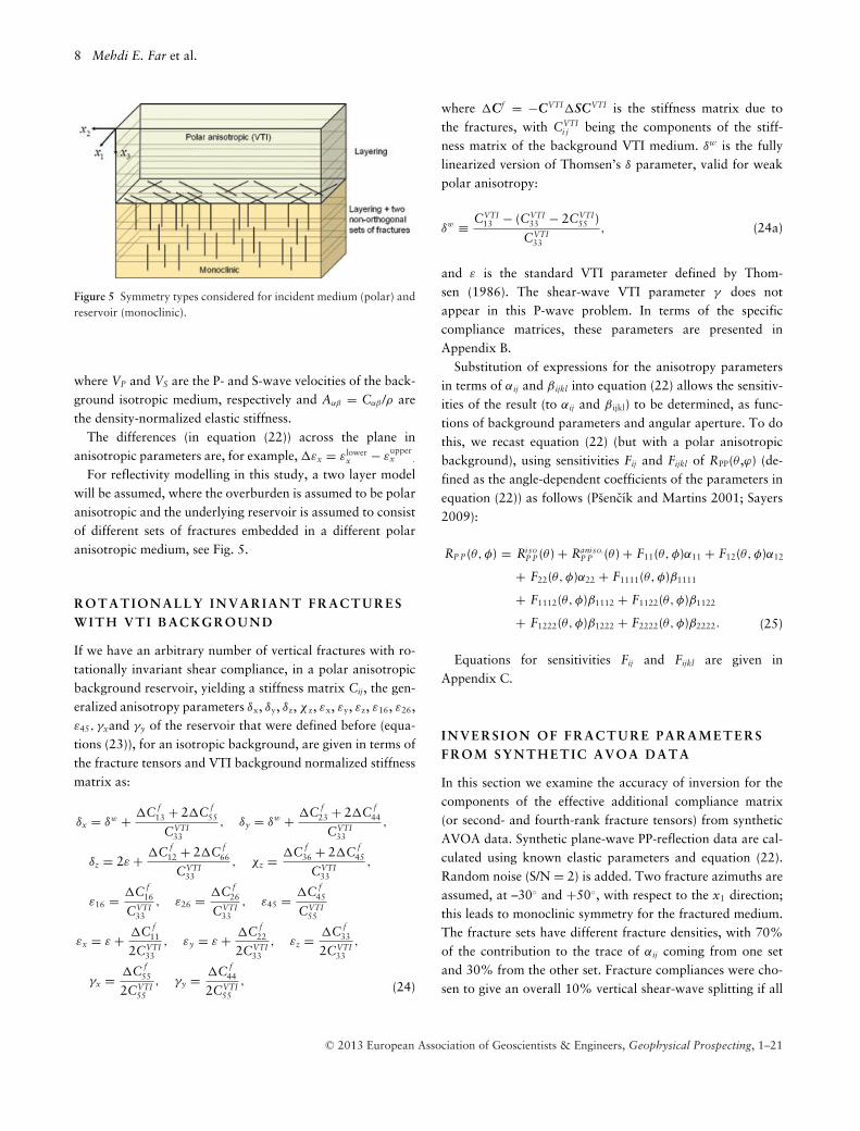
Figure 5 Symmetry types considered for incident medium (polar) andreservoir (monoclinic).

where VP and VS are the P- and S-wave velocities of the back-ground isotropic medium, respectively and Aαβ = Cαβ /ρ arethe density-normalized elastic stiffness.

The differences (in equation (22)) across the plane inanisotropic parameters are, for example, �εx = εlower

x − εupperx .

For reflectivity modelling in this study, a two layer modelwill be assumed, where the overburden is assumed to be polaranisotropic and the underlying reservoir is assumed to consistof different sets of fractures embedded in a different polaranisotropic medium, see Fig. 5.

ROTATIONALL Y I N V A R I A N T FR A C T URESW I T H V T I B A C K G R O U N D

If we have an arbitrary number of vertical fractures with ro-tationally invariant shear compliance, in a polar anisotropicbackground reservoir, yielding a stiffness matrix Cij, the gen-eralized anisotropy parameters δx, δy, δz, χ z, εx, εy, εz, ε16, ε26,ε45, γxand γy of the reservoir that were defined before (equa-tions (23)), for an isotropic background, are given in terms ofthe fracture tensors and VTI background normalized stiffnessmatrix as:

δx = δw + �C f13 + 2�C f

55

CVTI33

, δy = δw + �C f23 + 2�C f

44

CVTI33

,

δz = 2ε + �C f12 + 2�C f

66

CVTI33

, χz = �C f36 + 2�C f

45

CVTI33

,

ε16 = �C f16

CVTI33

, ε26 = �C f26

CVTI33

, ε45 = �C f45

CVTI55

εx = ε + �C f11

2CVTI33

, εy = ε + �C f22

2CVTI33

, εz = �C f33

2CVTI33

,

γx = �C f55

2CVTI55

, γy = �C f44

2CVTI55

, (24)

where �Cf = −CVTI�SCVTI is the stiffness matrix due tothe fractures, with CVTI

i j being the components of the stiff-ness matrix of the background VTI medium. δw is the fullylinearized version of Thomsen’s δ parameter, valid for weakpolar anisotropy:

δw ≡ CVTI13 − (CVTI

33 − 2CVTI55 )

CVTI33

, (24a)

and ε is the standard VTI parameter defined by Thom-sen (1986). The shear-wave VTI parameter γ does notappear in this P-wave problem. In terms of the specificcompliance matrices, these parameters are presented inAppendix B.

Substitution of expressions for the anisotropy parametersin terms of αij and β ijkl into equation (22) allows the sensitiv-ities of the result (to αij and β ijkl) to be determined, as func-tions of background parameters and angular aperture. To dothis, we recast equation (22) (but with a polar anisotropicbackground), using sensitivities Fij and Fijkl of RPP(θ ,ϕ) (de-fined as the angle-dependent coefficients of the parameters inequation (22)) as follows (Psencık and Martins 2001; Sayers2009):

RP P (θ, φ) = RisoP P (θ ) + Raniso.

P P (θ ) + F11(θ, φ)α11 + F12(θ, φ)α12

+ F22(θ, φ)α22 + F1111(θ, φ)β1111

+ F1112(θ, φ)β1112 + F1122(θ, φ)β1122

+ F1222(θ, φ)β1222 + F2222(θ, φ)β2222. (25)

Equations for sensitivities Fij and Fijkl are given inAppendix C.

I N V E R S I O N OF FR A C T U R E P A R A M E T E R SFROM SYNTHETIC AVOA D ATA

In this section we examine the accuracy of inversion for thecomponents of the effective additional compliance matrix(or second- and fourth-rank fracture tensors) from syntheticAVOA data. Synthetic plane-wave PP-reflection data are cal-culated using known elastic parameters and equation (22).Random noise (S/N = 2) is added. Two fracture azimuths areassumed, at –30◦ and +50◦, with respect to the x1 direction;this leads to monoclinic symmetry for the fractured medium.The fracture sets have different fracture densities, with 70%of the contribution to the trace of αij coming from one setand 30% from the other set. Fracture compliances were cho-sen to give an overall 10% vertical shear-wave splitting if all



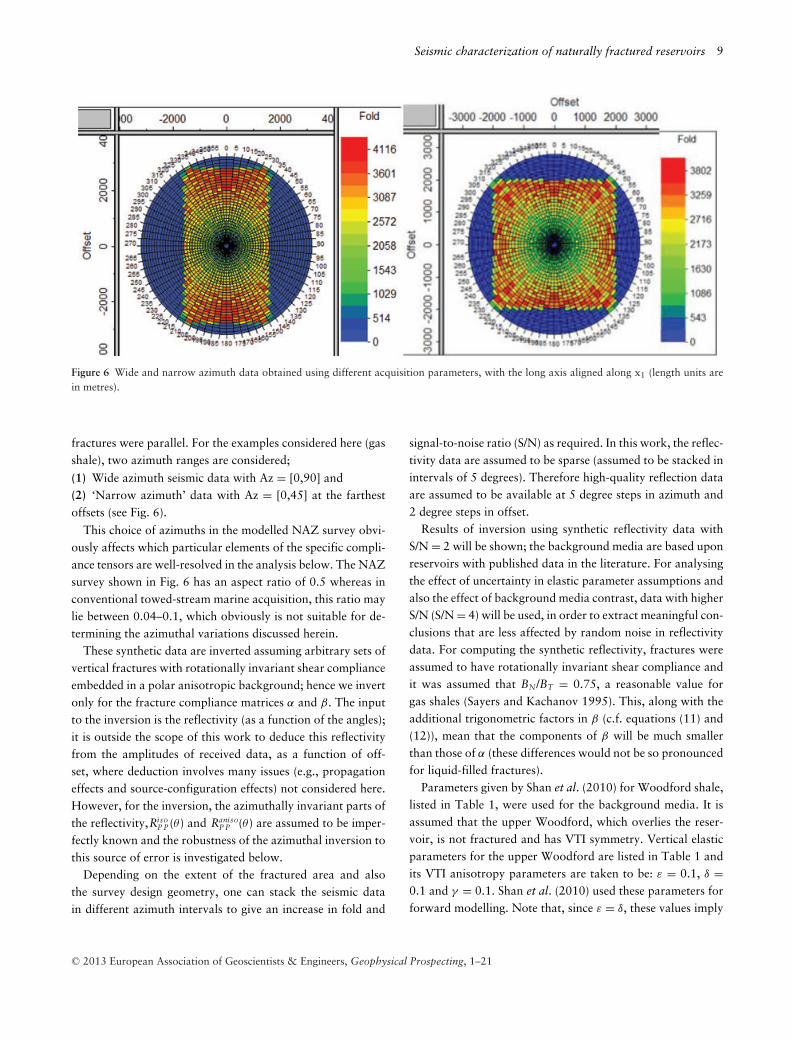
Figure 6 Wide and narrow azimuth data obtained using different acquisition parameters, with the long axis aligned along x1 (length units arein metres).

fractures were parallel. For the examples considered here (gasshale), two azimuth ranges are considered;

(1) Wide azimuth seismic data with Az = [0,90] and(2) ‘Narrow azimuth’ data with Az = [0,45] at the farthestoffsets (see Fig. 6).

This choice of azimuths in the modelled NAZ survey obvi-ously affects which particular elements of the specific compli-ance tensors are well-resolved in the analysis below. The NAZsurvey shown in Fig. 6 has an aspect ratio of 0.5 whereas inconventional towed-stream marine acquisition, this ratio maylie between 0.04–0.1, which obviously is not suitable for de-termining the azimuthal variations discussed herein.

These synthetic data are inverted assuming arbitrary sets ofvertical fractures with rotationally invariant shear complianceembedded in a polar anisotropic background; hence we invertonly for the fracture compliance matrices α and β. The inputto the inversion is the reflectivity (as a function of the angles);it is outside the scope of this work to deduce this reflectivityfrom the amplitudes of received data, as a function of off-set, where deduction involves many issues (e.g., propagationeffects and source-configuration effects) not considered here.However, for the inversion, the azimuthally invariant parts ofthe reflectivity,Riso

P P (θ ) and RanisoP P (θ ) are assumed to be imper-

fectly known and the robustness of the azimuthal inversion tothis source of error is investigated below.

Depending on the extent of the fractured area and alsothe survey design geometry, one can stack the seismic datain different azimuth intervals to give an increase in fold and

signal-to-noise ratio (S/N) as required. In this work, the reflec-tivity data are assumed to be sparse (assumed to be stacked inintervals of 5 degrees). Therefore high-quality reflection dataare assumed to be available at 5 degree steps in azimuth and2 degree steps in offset.

Results of inversion using synthetic reflectivity data withS/N = 2 will be shown; the background media are based uponreservoirs with published data in the literature. For analysingthe effect of uncertainty in elastic parameter assumptions andalso the effect of background media contrast, data with higherS/N (S/N = 4) will be used, in order to extract meaningful con-clusions that are less affected by random noise in reflectivitydata. For computing the synthetic reflectivity, fractures wereassumed to have rotationally invariant shear compliance andit was assumed that BN/BT = 0.75, a reasonable value forgas shales (Sayers and Kachanov 1995). This, along with theadditional trigonometric factors in β (c.f. equations (11) and(12)), mean that the components of β will be much smallerthan those of α (these differences would not be so pronouncedfor liquid-filled fractures).

Parameters given by Shan et al. (2010) for Woodford shale,listed in Table 1, were used for the background media. It isassumed that the upper Woodford, which overlies the reser-voir, is not fractured and has VTI symmetry. Vertical elasticparameters for the upper Woodford are listed in Table 1 andits VTI anisotropy parameters are taken to be: ε = 0.1, δ =0.1 and γ = 0.1. Shan et al. (2010) used these parameters forforward modelling. Note that, since ε = δ, these values imply



Table 1 Parameters for Woodford shale (Bayuk et al. 2009; Shan et al. 2010).

Woodford Shale Depth (km) Thickness (m) VPO [krn/s] VSO [km/s] VP0/VS0 Density (g/cc) ε δ γ

Upper ∼4 9.144 4.509 2.855 1.58 2.855 0.1 0.1 0.1Middle ∼4 53.34 4.161 2.687 1.55 2.46 0.29 0.17 0.1

elliptical P-wave fronts, which is a special case, not necessar-ily realistic, which leads to difficulties in converting reflectionarrival times to depths (Thomsen 1986). However, this doesnot create any difficulties in this study.

It is also assumed that the middle Woodford is the reservoirand has two sets of vertical and non-orthogonal fractures thatlead to monoclinic symmetry (see Fig. 5). Background elasticparameters for the middle Woodford are again selected fromTable 1 but anisotropy parameters are chosen from Bayuket al. (2009) who reported anisotropy parameters for 3 sam-ples from the Woodford shale that showed positive anellip-ticity (i.e., ε-δ > 0). Since their measurements for differentsamples agree with each other, background VTI anisotropyparameters measured by Bayuk et al. (2009) were used for themiddle Woodford: ε = 0.29, δ = 0.17 and γ = 0.1. These VTIparameters are not small, as strictly required by the presenttheory but this should not affect the present conclusions con-cerning azimuthal anisotropy, since any errors introduced bythe failure of the weak VTI approximation will have azimuthalisotropy. The symmetries of the upper and the middle Wood-ford are shown in Fig. 5.

The forward problem has the simple form

R = Fw, (26)

where R is a vector (of length N) containing all data (reflectioncoefficients), w is a vector (of length M) that represents theunknown parameters (components of the second- and fourth-rank fracture tensors) and F is the N × M sensitivity matrix.In this problem, M = 8. Inversion can be performed usingeither simple matrix operations, or, more robustly, using theconjugate gradient method that was used in this work. In thefirst case, the solution can be obtained from

w = (F T F )−1 F T R. (27)

Moreover, since for the present AVOA inversion it is as-sumed that the background (un-fractured) parameters areknown, statistical methods for inversion of elastic parametersfrom post-stack 3D surface seismic data can be used (e.g., Far2011). Since conventional seismic inversion for isotropic prop-erties will have some error and uncertainty involved, Monte

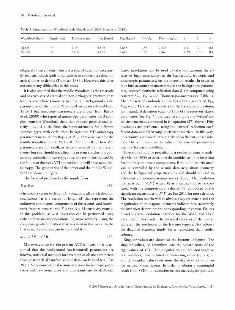
Carlo simulation will be used to take into account the ef-fects of high uncertainty, in the background isotropic andanisotropic parameters, on the inversion results. In order totake into account the uncertainty in the background parame-ters, ‘correct’ synthetic reflection data R are computed usingconstant VP0, VS0, ρ and Thomsen parameters (see Table 1).Then 50 sets of randomly and independently generated VP0,VS0, ρ and Thomsen parameters for the background medium,with standard deviation equal to 15% of the reservoir elasticparameters (see Fig. 7), are used to compute the ‘wrong’ co-efficient matrices contained in F (equation (27) above). Fiftyinversions are performed using the ‘correct’ reflection coef-ficient data and 50 ‘wrong’ coefficient matrices. In this way,uncertainty is included in the matrix of coefficients or sensitiv-ities. The red line shows the value of the ‘correct’ parametersused for forward modelling.

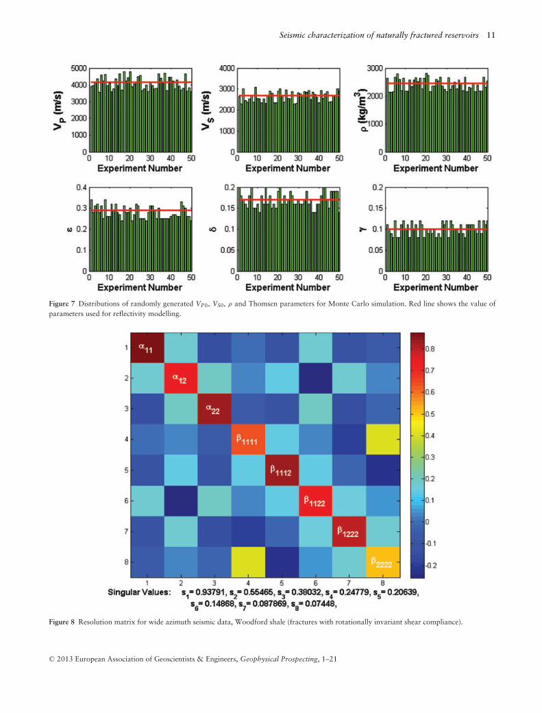
Inversion should be preceded by a resolution matrix analy-sis (Menke 1989) to determine the confidence in the inversionfor the fracture tensor components. Resolution matrix anal-ysis is controlled by the seismic data acquisition geometryand the background properties only and should be used todetermine an optimum seismic survey design. The resolutionmatrix is Rm = V pV T

p where VP is a matrix (not to be con-fused with the compressional velocity VP) composed of thesignificant eigenvalues of FTF (see Far 2011 for more details).The resolution matrix will be always a square matrix and themagnitudes of its diagonal elements indicate how accuratelythe inversion determines the corresponding unknown. Figures8 and 9 show resolution matrices for the WAZ and NAZdata used in this study. The diagonal elements of the matrixrepresent the resolution of the fracture tensors. Hot coloursfor diagonal elements imply better resolution than coolercolours.

Singular values are shown at the bottom of figures. Thesingular values, or s-numbers, are the square roots of theeigenvalues of FTF. The singular values are non-negativereal numbers, usually listed in decreasing order (s1 > s2 >

s3 . . .). Singular values determine the degree of variation inthe matrix of coefficients. In order to obtain a meaningfulresult from SVD and resolution matrix analysis, insignificant



Figure 7 Distributions of randomly generated VP0, VS0, ρ and Thomsen parameters for Monte Carlo simulation. Red line shows the value ofparameters used for reflectivity modelling.

Figure 8 Resolution matrix for wide azimuth seismic data, Woodford shale (fractures with rotationally invariant shear compliance).



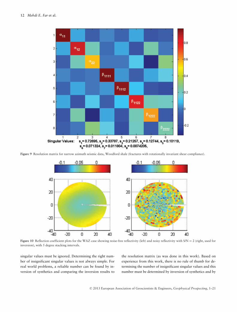
Figure 9 Resolution matrix for narrow azimuth seismic data, Woodford shale (fractures with rotationally invariant shear compliance).

Figure 10 Reflection coefficient plots for the WAZ case showing noise-free reflectivity (left) and noisy reflectivity with S/N = 2 (right, used forinversion), with 5 degree stacking intervals.

singular values must be ignored. Determining the right num-ber of insignificant singular values is not always simple. Forreal world problems, a reliable number can be found by in-version of synthetics and comparing the inversion results to

the resolution matrix (as was done in this work). Based onexperience from this work, there is no rule of thumb for de-termining the number of insignificant singular values and thisnumber must be determined by inversion of synthetics and by



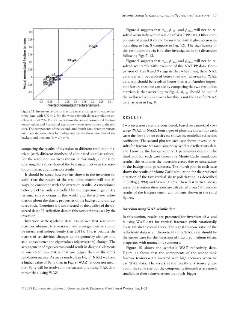
Figure 11 Inversion results of fracture tensors using synthetic reflec-tivity data with S/N = 2 for the wide azimuth data; correlation co-efficient = 98.9%. Vertical axes show the actual normalized fracturetensor values and horizontal axes show the inverted values of the ten-sors. The components of the second- and fourth-rank fracture tensorsare made dimensionless by multiplying by the shear modulus of thebackground medium (μ = ρVS0

2).

comparing the results of inversion to different resolution ma-trices (with different numbers of eliminated singular values).For the resolution matrices shown in this study, eliminationof 2 singular values showed the best match between the reso-lution matrix and inversion results.

It should be noted however (as shown in the inversion re-sults) that the results of the resolution matrix will not al-ways be consistent with the inversion results. As mentionedbefore, SVD is only controlled by the experiment geometry(seismic survey design in this work) and the a priori infor-mation about the elastic properties of the background unfrac-tured rock. Therefore it is not affected by the quality of the ob-served data (PP-reflection data in this work) that is used by theinversion.

Inversion with synthetic data has shown that resolutionmatrices, obtained from data with different geometries, shouldbe interpreted independently (Far 2011). This is because thematrix of sensitivities changes as the geometry changes andas a consequence the eigenvalues (eigenvectors) change. Thearrangement of eigenvectors could result in diagonal elementsin one resolution matrix that are bigger than in the otherresolution matrix. As an example, if in Fig. 9 (NAZ) we havea higher value of β1111 than in Fig. 8 (WAZ), it does not meanthat β1111 will be resolved more successfully using NAZ datarather than using WAZ.

Figure 8 suggests that α12, β1111 and β2222 will not be re-solved accurately with inversion of WAZ PP data. Other com-ponents of α and β should be inverted with higher accuraciesaccording to Fig. 8 (compare to Fig. 12). The significance ofthis resolution matrix is further investigated in the discussionfollowing Figs 7–12.

Figure 9 suggests that α22, β1222 and β2222 will not be re-solved accurately with inversion of this NAZ PP data. Com-parison of Figs 8 and 9 suggests that when using these NAZdata, α12 will be resolved better than α22, whereas for WAZdata, α22 should be resolved better than α12. Another impor-tant feature that one can see by comparing the two resolutionmatrices is that according to Fig. 9, β1111 should be one ofthe well-resolved unknowns but this is not the case for WAZdata, as seen in Fig. 8.

R E S U L T S

Two inversion cases are considered, based on azimuthal cov-erage (WAZ or NAZ). Four types of plots are shown for eachcase: the first plot for each case shows the modelled reflectioncoefficient. The second plot for each case shows inversion re-sults for fracture tensors using noisy synthetic reflectivity dataand knowing the background VTI parameters exactly. Thethird plot for each case shows the Monte Carlo simulationresults; this estimates the inversion errors due to uncertaintyin the background parameters. The fourth plot in each caseshows the results of Monte Carlo simulation for the predicteddirection of the fast vertical shear polarization, as describedin Helbig (1994) and Sayers (1998). These fast vertical shear-wave polarization directions are calculated from 50 inversionresults of the fracture tensor components shown in the thirdfigures.

Inversion using WAZ seismic data

In this section, results are presented for inversion of α andβ using WAZ data for vertical fractures (with rotationallyinvariant shear compliance). The signal-to-noise ratio of thereflectivity data is 2. Theoretically this WAZ case should bethe easiest case for the inversion of fractured medium elasticproperties with monoclinic symmetry.

Figure 10 shows the synthetic WAZ reflectivity data.Figure 11 shows that the components of the second-rankfracture tensors α are inverted with high accuracy when weuse WAZ data. The errors in the fourth-rank tensor β areabout the same size but the components themselves are muchsmaller, so their relative errors are much bigger.



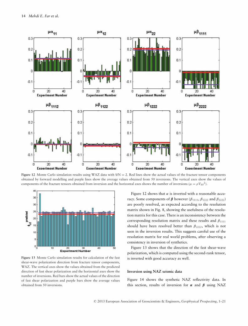
Figure 12 Monte Carlo simulation results using WAZ data with S/N = 2. Red lines show the actual values of the fracture tensor componentsobtained by forward modelling and purple lines show the average values obtained from 50 inversions. The vertical axes show the values ofcomponents of the fracture tensors obtained from inversion and the horizontal axes shows the number of inversions (μ = ρVS0

2).

Figure 13 Monte Carlo simulation results for calculation of the fastshear-wave polarization direction from fracture tensor components,WAZ. The vertical axes show the values obtained from the predicteddirection of fast shear polarization and the horizontal axes show thenumber of inversions. Red bars show the actual values of the directionof fast shear polarization and purple bars show the average valuesobtained from 50 inversions.

Figure 12 shows that α is inverted with a reasonable accu-racy. Some components of β however (β1111, β1222 and β2222)are poorly resolved, as expected according to the resolutionmatrix shown in Fig. 8, showing the usefulness of the resolu-tion matrix for this case. There is an inconsistency between thecorresponding resolution matrix and these results and β1111

should have been resolved better than β2222, which is notseen in the inversion results. This suggests careful use of theresolution matrix for real world problems, after observing aconsistency in inversion of synthetics.

Figure 13 shows that the direction of the fast shear-wavepolarization, which is computed using the second-rank tensor,is inverted with good accuracy as well.

Inversion using NAZ seismic data

Figure 14 shows the synthetic NAZ reflectivity data. Inthis section, results of inversion for α and β using NAZ



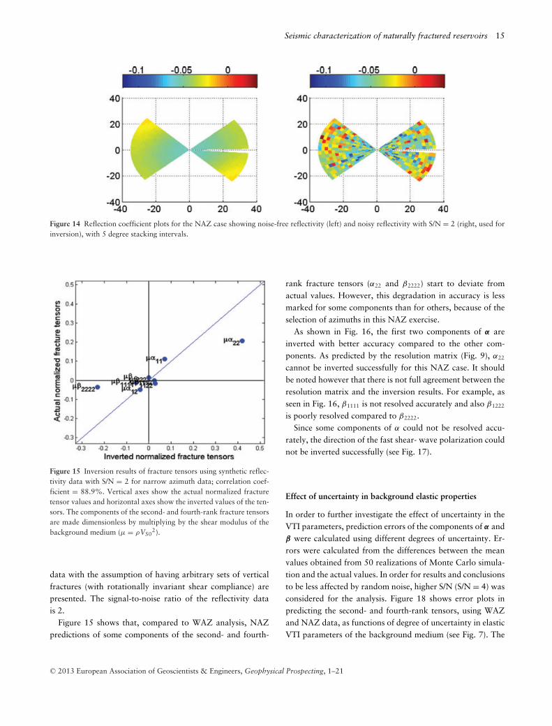
Figure 14 Reflection coefficient plots for the NAZ case showing noise-free reflectivity (left) and noisy reflectivity with S/N = 2 (right, used forinversion), with 5 degree stacking intervals.

Figure 15 Inversion results of fracture tensors using synthetic reflec-tivity data with S/N = 2 for narrow azimuth data; correlation coef-ficient = 88.9%. Vertical axes show the actual normalized fracturetensor values and horizontal axes show the inverted values of the ten-sors. The components of the second- and fourth-rank fracture tensorsare made dimensionless by multiplying by the shear modulus of thebackground medium (μ = ρVS0

2).

data with the assumption of having arbitrary sets of verticalfractures (with rotationally invariant shear compliance) arepresented. The signal-to-noise ratio of the reflectivity datais 2.

Figure 15 shows that, compared to WAZ analysis, NAZpredictions of some components of the second- and fourth-

rank fracture tensors (α22 and β2222) start to deviate fromactual values. However, this degradation in accuracy is lessmarked for some components than for others, because of theselection of azimuths in this NAZ exercise.

As shown in Fig. 16, the first two components of α areinverted with better accuracy compared to the other com-ponents. As predicted by the resolution matrix (Fig. 9), α22

cannot be inverted successfully for this NAZ case. It shouldbe noted however that there is not full agreement between theresolution matrix and the inversion results. For example, asseen in Fig. 16, β1111 is not resolved accurately and also β1222

is poorly resolved compared to β2222.Since some components of α could not be resolved accu-

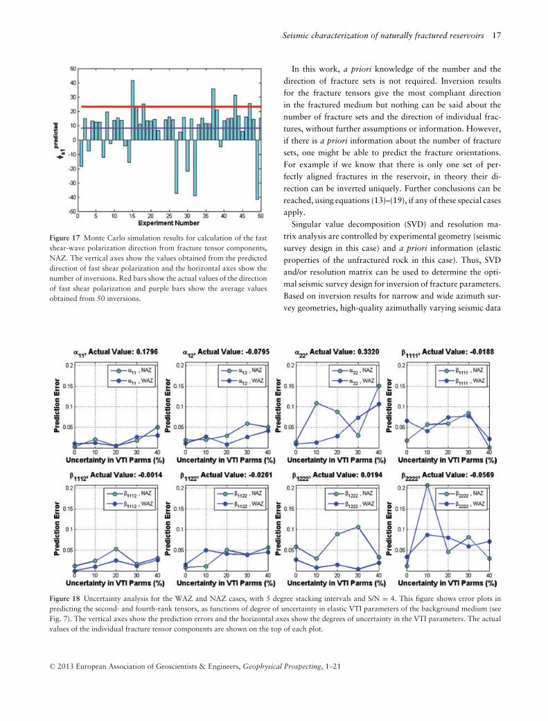
rately, the direction of the fast shear- wave polarization couldnot be inverted successfully (see Fig. 17).

Effect of uncertainty in background elastic properties

In order to further investigate the effect of uncertainty in theVTI parameters, prediction errors of the components of α andβ were calculated using different degrees of uncertainty. Er-rors were calculated from the differences between the meanvalues obtained from 50 realizations of Monte Carlo simula-tion and the actual values. In order for results and conclusionsto be less affected by random noise, higher S/N (S/N = 4) wasconsidered for the analysis. Figure 18 shows error plots inpredicting the second- and fourth-rank tensors, using WAZand NAZ data, as functions of degree of uncertainty in elasticVTI parameters of the background medium (see Fig. 7). The



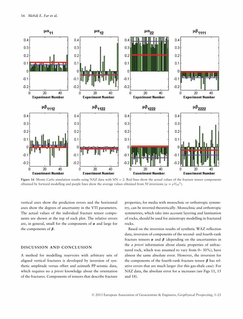
Figure 16 Monte Carlo simulation results using NAZ data with S/N = 2. Red lines show the actual values of the fracture tensor componentsobtained by forward modelling and purple lines show the average values obtained from 50 inversions (μ = ρVS0

2).

vertical axes show the prediction errors and the horizontalaxes show the degrees of uncertainty in the VTI parameters.The actual values of the individual fracture tensor compo-nents are shown at the top of each plot. The relative errorsare, in general, small for the components of α and large forthe components of β.

DISCUSS ION A N D C ON C L USI ON

A method for modelling reservoirs with arbitrary sets ofaligned vertical fractures is developed by inversion of syn-thetic amplitude versus offset and azimuth PP-seismic data,which requires no a priori knowledge about the orientationof the fractures. Components of tensors that describe fracture

properties, for media with monoclinic or orthotropic symme-try, can be inverted theoretically. Monoclinic and orthotropicsymmetries, which take into account layering and laminationof rocks, should be used for anisotropy modelling in fracturedrocks.

Based on the inversion results of synthetic WAZ reflectiondata, inversion of components of the second- and fourth-rankfracture tensors α and β (depending on the uncertainties inthe a priori information about elastic properties of unfrac-tured rock, which was assumed to vary from 0– 30%), havealmost the same absolute error. However, the inversion forthe components of the fourth-rank fracture tensor β has rel-ative errors that are much larger (for this gas-shale case). ForNAZ data, the absolute error for α increases (see Figs 11, 15and 18).



Figure 17 Monte Carlo simulation results for calculation of the fastshear-wave polarization direction from fracture tensor components,NAZ. The vertical axes show the values obtained from the predicteddirection of fast shear polarization and the horizontal axes show thenumber of inversions. Red bars show the actual values of the directionof fast shear polarization and purple bars show the average valuesobtained from 50 inversions.

In this work, a priori knowledge of the number and thedirection of fracture sets is not required. Inversion resultsfor the fracture tensors give the most compliant directionin the fractured medium but nothing can be said about thenumber of fracture sets and the direction of individual frac-tures, without further assumptions or information. However,if there is a priori information about the number of fracturesets, one might be able to predict the fracture orientations.For example if we know that there is only one set of per-fectly aligned fractures in the reservoir, in theory their di-rection can be inverted uniquely. Further conclusions can bereached, using equations (13)–(19), if any of these special casesapply.

Singular value decomposition (SVD) and resolution ma-trix analysis are controlled by experimental geometry (seismicsurvey design in this case) and a priori information (elasticproperties of the unfractured rock in this case). Thus, SVDand/or resolution matrix can be used to determine the opti-mal seismic survey design for inversion of fracture parameters.Based on inversion results for narrow and wide azimuth sur-vey geometries, high-quality azimuthally varying seismic data

Figure 18 Uncertainty analysis for the WAZ and NAZ cases, with 5 degree stacking intervals and S/N = 4. This figure shows error plots inpredicting the second- and fourth-rank tensors, as functions of degree of uncertainty in elastic VTI parameters of the background medium (seeFig. 7). The vertical axes show the prediction errors and the horizontal axes show the degrees of uncertainty in the VTI parameters. The actualvalues of the individual fracture tensor components are shown on the top of each plot.



with a high-fold number is required to characterize fracturesreliably.

REFERENCES

Bayuk I.O., Chesnokov E.M., Ammermann M. and Dyaur N. 2009.Elastic properties of four shales reconstructed from laboratory mea-surements at unloaded conditions. 79th SEG Annual Meeting, Ex-panded Abstracts.

Crampin S. 1984. Effective anisotropic constants for wave propa-gation through cracked solids. Geophysical Journal of the RoyalAstronomical Society 76, 135–145.

Eftekharifar M. and Sayers C.M. 2011a. Seismic characterization offractured reservoirs: A resolution matrix approach. 81st SEG An-nual Meeting, Expanded Abstracts.

Eftekharifar M. and Sayers C.M. 2011b. Seismic characterization offractured reservoirs: Inversion for fracture parameters illustratedusing synthetic AVOA data. 81st SEG Annual Meeting, ExpandedAbstracts.

Far M.E. 2011. Seismic Characterization of Naturally FracturedReservoirs. PhD dissertation, University of Houston, Houston, TX.

Grechka V. and Kachanov M. 2006. Effective elasticity of rockswith closely spaced and intersecting cracks. Geophysics 71, 85–91.

Helbig K. 1994. Foundations of Elastic Anisotropy for ExplorationSeismic. Pergamon Press.

Hill R. 1963. Elastic properties of reinforced solids: Some theoreti-cal principles. Journal of the Mechanics and Physics of Solids 11,357–372.

Jones J.P. and Whittier J.S. 1967. Waves at a flexibly bonded interface.Journal of Applied Mechanics 34, 905–909.

Kachanov M. 1980. Continuum model of medium with cracks.Journal of the Engineering Mechanics Division of the Amer-ican Society of Civil Engineers 106, no. EMS5, 1039–1051.

Lynn H.B., Bates C.R., Layman M. and Jones M. 1994. Naturalfracture characterization using P-wave reflection seismic data, VSP,borehole imaging logs, and in-situ stress field determination. SPE29595.

Mallick S., Chambers R. E. and Gonzalez A. 1996. Method for de-termining the principal axes of azimuthal anisotropy from seismicP-wave data. US Patent 5508973.

Menke W. 1989. Geophysical Data Analysis: Discrete Inverse The-ory. Academic Press.

Nelson R.A. 1985. Geologic Analysis of Naturally Fractured Reser-voirs. Gulf Publishing Company, Houston.

Nichols D., Muir F. and Schoenberg M. 1989. Elastic properties ofrocks with multiple sets of fractures. 59th SEG Annual Meeting,Expanded Abstracts.

Psencık I. and Martins J.L. 2001. Properties of weak contrastPP reflection/transmission coefficients for weakly anisotropicelastic media. Studia Geophysica et Geodaetica 45, 176–199.

Reiss L.H. 1980. The Reservoir Engineering Aspects of FracturedFormations. Editions Technip, Paris.

Rueger A. 1997. P-wave reflection coefficients for transverselyisotropic media with vertical and horizontal axis of symmetry. Geo-physics 62, 713–722.

Sayers C.M. 1998. Misalignment of the orientation of fractures andthe principal axes for P- and S-waves in rocks containing multi-ple non-orthogonal fracture sets. Geophysical Journal International133, 459–466.

Sayers C.M. 2009. Seismic characterization of reservoirs contain-ing multiple fracture sets. Geophysical Prospecting 57, 187–192.

Sayers C.M. and Dean S. 2001. Azimuth-dependent AVO in reservoirscontaining non-orthogonal fracture sets. Geophysical Prospecting49, 100–106.

Sayers C.M. and Kachanov M. 1991. A simple technique for find-ing effective elastic constants of cracked solids for arbitrary crackorientation statistics. International Journal of Solids and Structures12, 81–97.

Sayers C.M. and Kachanov M. 1995. Microcrack-induced elasticwave anisotropy of brittle rocks. Journal of Geophysical Research100, 4149–4156.

Sayers C.M. and Rickett J.E. 1997. Azimuthal variation in AVOresponse for fractured gas sands. Geophysical Prospecting 45,165–182.

Schoenberg M. 1980. Elastic wave behavior across linear slip in-terfaces. Journal of the Acoustical Society of America 68, 1516–1521.

Schoenberg M. and Muir F. 1989. A calculus for finely layeredanisotropic media. Geophysics 54, 581–589.

Schoenberg M. and Sayers C.M. 1995. Seismic anisotropy of fracturedrock. Geophysics 60, 204–211.

Shan N., Tatham R., Sen M.K., Spikes K. and RuppelS.C. 2010. Sensitivity of seismic response to variations inthe Woodford Shale. 80th SEG Annual Meeting, ExpandedAbstracts.

Thomsen L. 1986. Weak elastic anisotropy. Geophysics 51,1954–1966.

Thomsen L. 1995. Elastic anisotropy due to aligned cracks in porousrock. Geophysical Prospecting 43, 805–829.

Worthington M.H. 2008. Interpreting seismic anisotropy in fracturedreservoirs. First Break 26, 57–63.

APPENDIX A

SPECIAL CASES

Consider an isotropic background with one set of frac-tures aligned with x1 (x2 along the symmetry axis); this isthe principal coordinate system. Substituting the backgroundcompliance tensor (the first term on the right-hand side ofequation (6)) and the additional compliance tensor (the sec-ond term on the right-hand side of equation (6), cf. equa-tions (11) and (12) with cos ϕ = 1), in 2-index form, one



obtains:

S = 1E

⎡⎢⎢⎢⎢⎢⎢⎢⎢⎢⎢⎢⎣

1 −ν −ν 0 0 0

−ν 1 −ν 0 0 0

−ν −ν 1 0 0 0

0 0 0 2(1 + ν) 0 0

0 0 0 0 2(1 + ν) 0

0 0 0 0 0 2(1 + ν)

⎤⎥⎥⎥⎥⎥⎥⎥⎥⎥⎥⎥⎦

+

⎡⎢⎢⎢⎢⎢⎢⎢⎢⎢⎢⎢⎣

0 0 0 0 0 0

0 α22 + β2222 0 0 0 0

0 0 0 0 0 0

0 0 0 α22 0 0

0 0 0 0 0 0

0 0 0 0 0 α22

⎤⎥⎥⎥⎥⎥⎥⎥⎥⎥⎥⎥⎦

=

⎡⎢⎢⎢⎢⎢⎢⎢⎢⎢⎢⎢⎢⎢⎢⎣

1E

−ν/E −ν/E 0 0 0

−ν/E1E

+ α22 + β2222 −ν/E 0 0 0

−ν/E −ν/E1E

0 0 0

0 0 0 α22 + 2(1 + ν)/E 0 0

0 0 0 0 2(1 + ν)/E 0

0 0 0 0 0 α22 + 2(1 + ν)/E

⎤⎥⎥⎥⎥⎥⎥⎥⎥⎥⎥⎥⎥⎥⎥⎦

(A1)

which has HTI symmetry (Schoenberg and Sayers 1995). Sim-ilarly, one can show that, if the background medium is polaranisotropic, this one set of fractures results in orthotropicsymmetry. Similar methods prove that two orthogonal frac-ture sets (equations (14) and (15)) in an isotropic or polaranisotropic background medium result in orthotropic sym-metry and that two non-orthogonal fracture sets (equations(16) and (17)) in an isotropic or polar anisotropic backgroundmedium result in monoclinic symmetry.

APPENDIX B

GENERALIZED ANISOTROPY PARAMETERS

In terms of the specific compliance matrices, anisotropy pa-rameters are defined as (with the superscripts VTI for the back-ground polar anisotropic medium implicit):

εx = ε + −C211(α11 + β1111) − C2

12(α22 + β2222) − 2C11C12β1122

2C33

εy = ε + −C212(α11 + β1111) − C2

11(α22 + β2222) − 2C11C12β1122

2C33

εz = −C213(α11 + β1111 + α22 + β2222 + 2β1122)

2C33

ε16 = −C66(2C11β1112 + 2C12β1222 + α12(C11 + C12))C33

ε26 = −C66(2C12β1112 + 2C11β1222 + α12(C11 + C12))C33

ε45 = −C245α12

C55

δx = δw + −C13(C11(α11 + β1111) + C12(α22 + β2222) + β1122(C11 + C12)) − 2C255α11

C33



δy = δw + −C13(C12(α11 + β1111) + C11(α22 + β2222) + β1122(C11 + C12)) − 2C255α22

C33

δz = 2ε + C11C12(α11 + β1111 + α22 + β2222) − β1122(C11 + C12) − 2C266(α11 + α22 + 4β1122)

C33

γx = −C55α11

2(B1)

γy = −C55α22

2

χz = −2C66C13(α12 + β1112 + β1222) − 2C255α12

C33

APPENDIX C

SENSITIV ITY EQUA T I ON S

Sensitivities in equation (25) are obtained as:

F11(θ, φ) = 1μ

[− C2

13

4C33+

(cos2 φ

(−C11C13 + 2C2

55

C33

+ 4C55V2S

V2P

)− C12C13 sin2 φ

C33

)12

sin2 θ

+(

−C211 cos4 φ

2C33− (C11C12 + 2C2

66) cos2 φ sin2 φ

C33

− C212 sin4 φ

2C33

)12

sin2 θ tan2 θ

]

F12(θ, φ) = 1μ

[(4C55V2

S

V2P

− 2C255 + 2C13C66

C33

)sin φ cos φ sin2 θ

+(

− (C11 + C12)C66

C33

)cos φ sin φ sin2 θ tan2 θ

]

F22(θ, φ) = 1μ

[− C2

13

4C33+ 1

2

[−C12C13 cos2 φ

C33

+(

4C55V2S

V2P

+ −C11C13 − C255

C33

)]sin2 φ sin2 θ

+ 12

(− (C12 cos2 φ + C11 sin2 φ)2

2C33

− 2(C66 cos φ sin φ)2

C33

)sin2 θ tan2 θ

](C1)

F1111(θ, φ) = 1μ

[− C2

13

4C33+ 1

2

(−C13(C12 sin2 φ + C11 cos2 φ)

C33

)

× sin2 θ − 12

(1

2C33(C11 cos2 φ + C12 sin2 φ)2

)

× sin2 θ tan2 θ

]

F1112(θ, φ) = 1μ

[− 2C13C66 cos φ sin φ

C33sin2 θ

−(

2C66(C11 cos2 φ + C12 sin2 φ)C33

)

× cos φ sin φ sin2 θ tan2 θ

]

F1122(θ, φ) = 1μ

[− C2

13

2C33+ 1

2

×(

C13(C11 + C12)(2 cos2 φ − 1)C33

)sin2 θ

+ 12

(−C11C12 + (3(C11 − C12)2) cos2 φ sin2 φ

C33

)

× sin2 θ tan2 θ

]

F1222(θ, φ) = 1μ

[− 2C66C13

C33sin φ cos φ sin2 θ

+(

−2C66(C11 sin2 φ + C12 cos2 φ)C33

)

× sin φ cos φ sin2 θ tan2 θ

]



F2222(θ, φ) = 1μ

[− C2

13

4C33+ 1

2

×(

−C13(C11 sin2 φ + C12 cos2 φ)C33

)sin2 θ

+12

(− (C12 cos2 φ + C11 sin2 φ)2

2C33

)sin2 θ tan2 θ

]

where VP = VP01+VP022 , VS = VS01+VS02

2 are the average proper-ties of the upper and lower media and μ = ρVS0

2. For thespecial case of an isotropic background, the sensitivity rela-tions, fully linearized, simplify to:

F11(θ, φ) = 1μ

[− λ2

4M− 1

2

(cos2 φ

(λ2 + 2λμ − 2μ2

M

)

+ λ2 sin2 φ

M

)sin2 θ − 1

2

(12

M cos4 φ

+ (λM + 2μ2) sin2 φ cos2 φ

M+ λ2 sin4 φ

2M

)

× sin2 θ tan2 θ

]

F12(θ, φ) = 1μ

[ (−2μ(λ − μ)

M

)sin φ cos φ sin2 θ

− 2μ(λ + μ)M

cos φ sin φ sin2 θ tan2 θ

]

F22(θ, φ) = 1μ

[− λ2

4M+ 1

2

((−λ2 + 2λμ − 2μ2

M

)sin2 φ

+ λ2

2M(1 − 2 cos2 φ)

)sin2 θ

+12

(−λ2 cos4 φ

2M− (λM + 2μ2) sin2 φ cos2 φ

M

− 12

M sin4 φ

)sin2 θ tan2 θ

](C2)

F1111(θ, φ) = 1μ

[− λ2

4M+ 1

2

(−λ2 sin2 φ

M− λ cos2 φ + λ2

2M

)

× sin2 θ + 12

(−λ2 sin4 φ

2M

−12

M cos4 φ − λ sin2 φ cos2 φ

)sin2 θ tan2 θ

]

F1112(θ, φ) = 1μ

[− 2μλ

Mcos φ sin φ sin2 θ −

(2μλ sin2 φ

M

+ 2μ cos2 φ

)cos φ sin φ × sin2 θ tan2 θ

]

F1122(θ, φ) = 1μ

[− λ2

2M− 1

2

(λ(λ + 2μ)

M

)sin2 θ

+12

(− (λ2 + M2 + 4μ2) sin2 φ cos2 φ

M

− λ(sin4 φ + cos4 φ))

sin2 θ tan2 θ

]

F1222(θ, φ) = 1μ

[− 2λμ

Msin φ cos φ sin2 θ −

(2λμ cos2 φ

M

+ 2μ sin2 φ

)sin φ cos φ × sin2 θ tan2 θ

]

F2222(θ, φ) = 1μ

[− λ2

4M+ 1

2

(−λ sin2 φ + λ2

2M(1 − 2 cos2 φ)

)

× sin2 θ + 12

(− λ2 cos4 φ

2M− 1

2M sin4 φ

− λ sin2 φ cos2 φ

)sin2 θ tan2 θ

]

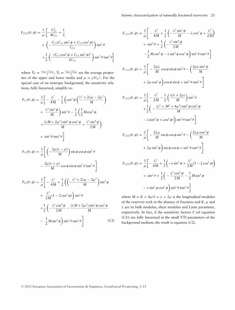
where M = K + 4μ/3 = λ + 2μ is the longitudinal modulusof the reservoir rock in the absence of fractures and K, μ andλ are its bulk modulus, shear modulus and Lame parameter,respectively. In fact, if the sensitivity factors F (of equation(C1)) are fully linearized in the small VTI parameters of thebackground medium, the result is equation (C2).


seismic characterization of naturally fractured reservoirs ... · pdf filegeophysical...

Documents