rate decline analysis for naturally fractured reservoirs … · rate decline analysis for naturally...
TRANSCRIPT
RATE DECLINE ANALYSIS FOR NATURALLY FRACTURED RESERVOIRS
A REPORT SUBMITTED TO THE DEPARTMENT OF PETROLEUM
.. ENGINEERING OF STANFORD UNIVERSITY
IN PARTIAL FULFILLMENT OF THE REQUIREMENTS FOR THE DEGREE OF MASTER OF SCIENCE
BY Katsunori Fujiwara
June 1989

I certify that I have read this report and that in my opinion it is fully adequate, in scope and in quality, as partial fulfillment of the degree of Master of Science in Petroleum Engineerihg.
?'/'Cp- -jJL - fq.4' Younes Jalali-Yazdi - (Principal advisor)
.. 11
Acknowledgement
I would like to thank Dr. Y o u w Jalali-Yazdi for his essential help and his able guidance as my research advisor during the come of this research work and the preparation of this report.
I also would like to thank the faculty, students, and staff of the Department of Petroleum Engineering for providing me with encouragement and good basis for research work.
I would like to dedicate the pzesent study to my wife, Rinko, for providing me patience and happiness.
Finally, I would like to thank Mippon Mining Co., Ltd. and Japan National Oil Corporation for having provided the financial support for my Master’s program at Stanford University.
... 111
Abstract
In this work, transient rate analylsiis for constant pressure production in a naturally fractured reservoir is presented. The solution for the dimensionless flowrate is based on a model which treats interporosity flow as a function of a continuous matrix block size distribution. Several distributions of matrix block size are considered. This approach is similar to that of Ref. 1, which examined the pressure response.
The flowrate response js investigated for both pseudo-steady state (PSS) and unsteady state (USS) interporosity models, which include slab, cylindrical, and spherical matrix block geometries, It was found that the flowrate decline becomes smooth, specially for the Gteadly state model, and approaches the decline behavior of a nonfractured reservoir when matrix block size Variability is large, i.e., when fracturing is extremely nonuniform. The difference in flowrate for various geometric models of blocks is not significant, with the spherical geometry yielding the highest and the slab yielding the lowest flowrate.
This work suggests why certain naturally fractured reservoirs do not exhibit a sudden rate decline followed by a period of constant flowrate as predicted by clas- sical double porosity models. Also, the results indicate that reservoir producibility is directly proportional to fracture intensity and inversely proportional to the de- gree of fracture nonunifonnity. Hence, the Warren and Root model which assumes fracturing is perfectly unifom, provides an upper bound of reservoir producibility and cumulative production.
iv
Contents
Acknowledgement iii
Abstract iv
Table of Contents vi
List of Tables vii
List of Figures ix
1 Introduction 1
2 Mathematical Model 4
2.1 Initial Boundary Value Problem . . . . . . . . . . . . . . . . . . . . . 4
2.2 Probability Density Functions (PDF) . . . . . . . . . . . . . . . . . . 6 2.3 Solutions . . . . . . . . . . . . . . . . . . . . . . . . . . . . . . . . 8
2.3.1 General Soluticm . . . . . . . . . . . . . . . . . . . . . . . . . 8 2.3.2 Solutions for Sllab Geometry . . . . . . . . . . . . . . . . . . . 8
2.3.3 Solutions for CylrSndrical Geometry . . . . . . . . . . . . . . . 11 2.3.4 Solutions for Spherical Geometry . . . . . . . . . . . . . . . . 11 2.3.5 Dimensionless Parameters . . . . . . . . . . . . . . . . . . . . 12
3 Discussion 15 3.1 Effect of Matrix Block Geometry . . . . . . . . . . . . . . . . . . . . 15
3.2 Effect of the Mode of Interporosity Flow . . . . . . . . . . . . . . . . 26
V
3.3 Effect of PDF Type . . . . . . . . . . . . . . . . . . . . . . . . . . . 29 3.4 Effect of Fracture Intensity and Uniformity . . . . . . . . . . . . . . 34
4 Conclusion 39
Nomenclature 41
Bibliography 45
A Derivation of Solution 48 A . l Slab Geometry . . . . . . . . . . . . . . . . . . . . . . . . . . . . . . 48
A . l . l Unsteady State . . . . . . . . . . . . . . . . . . . . . . . . . . 48 A.1.2 Pseudo-Steady State . . . . . . . . . . . . . . . . . . . . . . . 51
A.2 Cylindrical Geometry . . . . . . . . . . . . . . . . . . . . . . . . . . 53 A.2.1 Unsteady State . . . . . . . . . . . . . . . . . . . . . . . . . . 53 A.2.2 Pseudo-Steady State . . . . . . . . . . . . . . . . . . . . . . . 54
A.3 Spherical Geometry . . . . . . . . . . . . . . . . . . . . . . . . . . . 55 A.3.1 Unsteady State . . . . . . . . . . . . . . . . . . . . . . . . . . 55 A.3.2 Pseudo-Steady $tate . . . . . . . . . . . . . . . . . . . . . . . 57
B Computer Programs 59
vi
List of Tables
2.1 Constant Q for various matrix geometries . . . . . . . . . . . . . . . 13
vii
List of Figures
1.1 Naturally Fractured Reservoir . . . . . . . . . . . . . . . . . . . . . . 3
2.1 Uniform Distribution . . . . . . . . . . . . . . . . . . . . . . . . . . . 6 2.2 Positively Skewed Linear Distribution . . . . . . . . . . . . . . . . . 7 2.3 Negatively Skewed Linear Distribution . . . . . . . . . . . . . . . . . . 7 2.4 Matrix Slab Geometry . . . . . . . . . . . . . . . . . . . . . . . . . . 13 2.5 Matrix Cylindrical Geometry . . . . . . . . . . . . . . . . . . . . . . 14
2.6 Matrix Spherical Geomdry . . . . . . . . . . . . . . . . . . . . . . . 14
3.1 Flowrate profile for slab geometry in USS model . . . . . . . . . . . 17 3.2 Flowrate profile for cyEodrical geometry in USS model . . . . . . . . 18 3.3 Flowrate profile for spherical geometry in USS model . . . . . . . . . 19
3.5 Difference in flowrate of various matrix block geometries . . . . . . . 21 3.4 Comparison of flowrate tesponse of various matrix block geometries . 20
3.6 Pressure and pressure derivative profile for slab geometry in USS model . . . . . . . . . . . . . . . . . . . . . . . . . . . . . . . . . . . 22
3.7 Pressure and pressure derivative profile for cylindrical geometry in USS model . . . . . . . . . . . . . . . . . . . . . . . . . . . . . . . . 23
3.8 Pressure and pressure derivative profile for spherical geometry in USS model . . . . . . . . . . . . . . . . . . . . . . . . . . . . . . . . . . . 24
3.9 Comparison of pressure derivative profile of various matrix block ge- ometries . . . . . . . . . . . . . . . . . . . . . . . . . . . . . . . . . . 25
3.10 Comparison of PSS and WSS flowrate response . . . . . . . . . . . . 27 3.11 Comparison of PSS and USS pressure derivative profiles . . . . . . . 28
viii
... *.. ..
3.12 PSS flowrate profile for various matrix block size distributions . . . . 3.13 PSS pressure and pressure derivative profile for various matrix block
size distributions . . . . . . . . . . . . . . . . . . . . . . . . . . . . . 3.14 USS flowrate profile for parious matrix block size distributions . . . 3.15 USS pressure and pressure derivative profile for various matrix block
size distributions . . . . . . . . . . . . . . . . . . . . . . . . . . . . . 3.16 Cumdative production at t D = lo5 for Pss model . . . . . . . . . . 3.17 Cumdative production at t D = lo5 for uss model . . . . . . . . . . 3.18 Flowrate profile for various A . . . . . . . . . . . . . . . . . . . 3.19 Pressure derivative profile for various Xgmean . . . . . . . . . . . . . .
30
31 32
33 35 36 37 38
ix
Section 1
Introduction
Much work has been done on the pressure transient modeling of naturally fractured reservoirs. However, the rate response and producing capacity of these reservoirs have not received adequate attention. This work examines flowrate decline behavior of naturally fractured reservoirs.
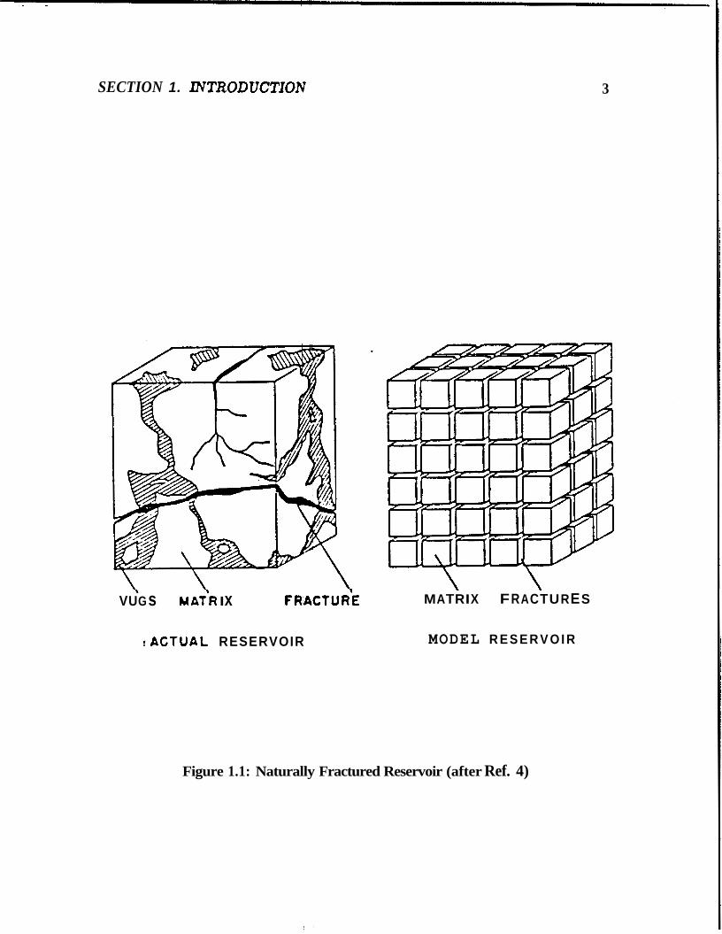
Naturally fractured reservoirs are heterogeneous porous media which consist of fractures and matrix blocks. The matrix blocks store most of the fluid, but have low permeability. On the other band, the fractures do not store much, but have extremely high permeability. Most of the reservoir fluid flows from the matrix blocks into the wellbore through the permeable fractures. Therefore, the produc- ing capacity of a naturally fractured reservoir is governed by matrix-fracture fluid transport capacity, which is called interporosity flow. To describe flow in naturally fractured reservoirs, double pomsity model has been widely used. Fig. 1.1 shows the schematic of a naturally fractured reservoir and its double porosity idealiza- tion. This concept was first proposed by Barenblatt et a1 [2,3). Transient pressure behavior for this model has been studied by many researchers [2-161. Mavor and Cinco-Ley [lo] and Da Prat e t a1 [17] examined the rate response of this model by applying the rate decline concept proposed by Fetkovich [18]. Raghavan and Ohaeri [19], and Sageev [ZO] also examined the rate dedine behavior of naturally fractured reservoirs. These work indicate that the double porosity model predicts an initial high flowrate followed by P sudden rate decline and a period of constant
1
SECTION I. INTRODUCTION 2
flowrate (the interporosity flow period). Although many naturally fractured reser- voirs exhibit such behavior, many others do not. They exhibit a gradual rate decline throughout the life of the reservoir, similar to that of nonfractured reservoirs. Jalali- Yazdi et a2 [21] suggested the concept of a distributed interporosity flow strength to explain such behavior.
Here, a similar approach is &dopted, and the effect of the variation of matrix block size on flowrate is investigated. This work demonstrates that the gradual rate decline occurs in nonuniformly fractured reservoirs where the variation in matrix block size is large. Also, this work shows that fracture nonuniformity has an adverse effect on the producing capacity of naturally fractured reservoirs.
SECTION 1. XNTRODUCTIOW
VUG s M ATR I x FRACTURE
:ACTUAL RESERVOIR
3
MATRIX FRACTURES
MODEL R E S E R V O I R
Figure 1.1: Naturally Fractured Reservoir (after Ref. 4)
Section 2
Mat hernatical Model
The partial differential equations and their solutions for pseudo-steady state and three unsteady state cases, which include slab, cylindrical, and spherical matrix block geometries, are presented in this section. Also, the probability density func- tions (PDF) used in this study to represent various distributions of matrix block size, are presented.
2.1 Initial Boundary Value Problem
The fracture diffusivity equatian for a double porosity reservoir with a continuous matrix block size distribution is given by:
and the matrix diffusivity equation is:
In Eqn. 2.1, P(h ) is the probability density function of matrix block size and is discussed in the next section. U ( h ) in Eqn. 2.1 is the flow contribution from a matrix block of size h, and is given by:
4
SECTION 2. MATHEMATICAL MODEL
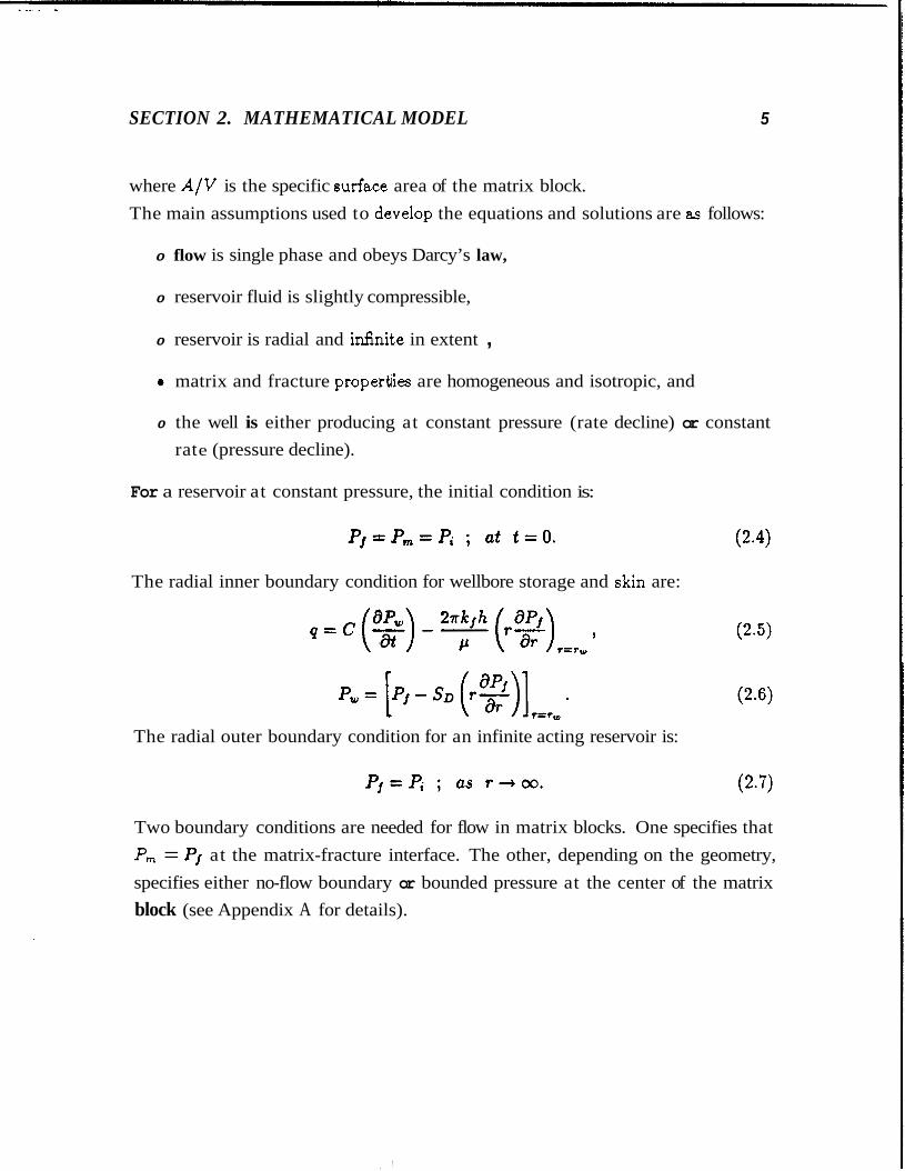
where A/V is the specific surfaae area of the matrix block.
5
The main assumptions used to develop the equations and solutions are as follows:
0 flow is single phase and obeys Darcy’s law,
0 reservoir fluid is slightly compressible,
0 reservoir is radial and idki te in extent ,
0 matrix and fracture properkies are homogeneous and isotropic, and
0 the well is either producing at constant pressure (rate decline) or constant rat e (pressure decline).
For a reservoir at constant pressure, the initial condition is:
The radial inner boundary condition for wellbore storage and skin are:
r=rw
The radial outer boundary condition for an infinite acting reservoir is:
Two boundary conditions are needed for flow in matrix blocks. One specifies that P, = Pi at the matrix-fracture interface. The other, depending on the geometry, specifies either no-flow boundary or bounded pressure at the center of the matrix block (see Appendix A for details).
SECTION 2. MATHEMATICAL MODEL 6
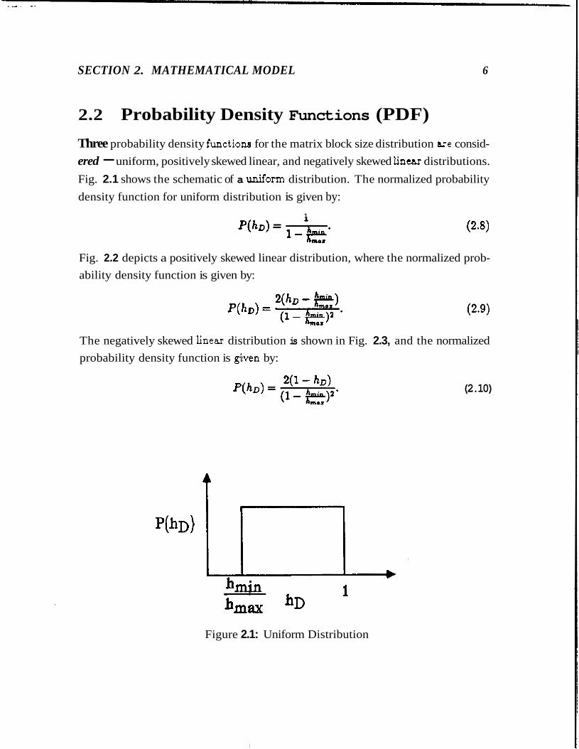
2.2 Probability Density Functions (PDF) Three probability density functions for the matrix block size distribution are consid- ered - uniform, positively skewed linear, and negatively skewed linear distributions. Fig. 2.1 shows the schematic of a uniform distribution. The normalized probability density function for uniform distribution is given by:
1
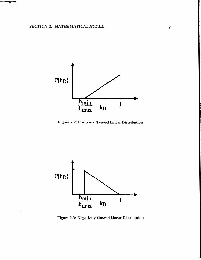
Fig. 2.2 depicts a positively skewed linear distribution, where the normalized prob- ability density function is given by:
The negatively skewed linear distribution is shown in Fig. 2.3, and the normalized probability density function is given by:
t
Figure 2.1: Uniform Distribution
(2.10)
SECTION 2. MATHEMATICAL MODEL
t
Figure 2.2:
t
Poaitively Skewed Linear Distribution
Figure 2.3: Negatively Skewed Linear Distribution
7
SECTION 2. MATHEMATICAL MODEL 8
2.3 Solutions
2.3.1 General Solution
The initial boundary value problem is rendered dimensionless and solved using Laplace transforms. The procedure is stated in Appendix A. The constant pressure solution is obtained from the constant rate solution (with CD = 0) using the result presented by van Everdingen and Hurst [22]:
(2.11)
Or, in Laplace space: - Q D = -. QD
S
The argument x of modified Bessel functions is:
x = Ja.
(2.13)
(2.14)
(2.15)
The function g(s) can be obtained by specifying the mode of interporosity flow (PSS or USS), the geometry of matrix blocks (slab, cylinder, or sphere), and the distribution of matrix block size.
2.3.2 Solutions for Slab Geometry
Fig. 2.4 shows the schematic of the slab geometry. In this geometry, matrix blocks and fractures are assumed to be piled up on one another. No flow boundary ex- ists at the center of the matrix slab due to flow symmetry. Pseudo-steady state
and unsteady state cases are considered for the three probability density functions discussed in section 2.2.
SECTION 2. MATHEMATICAL MODEL 9
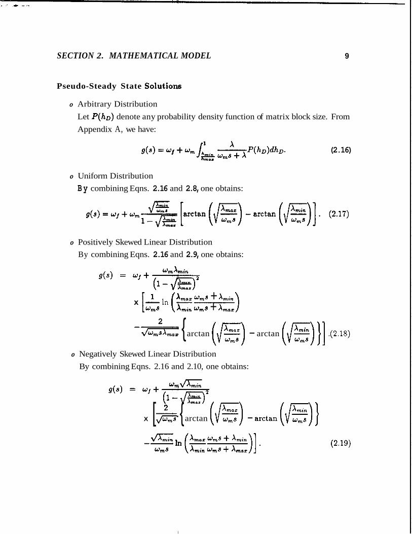
Pseudo-Steady State Solutiorus
0 Arbitrary Distribution Let P ( ~ D ) denote any probability density function of matrix block size. From Appendix A, we have:
(2.16)
0 Uniform Distribution B y combining Eqns. 2.16 and 2.8, one obtains:
0 Positively Skewed Linear Distribution By combining Eqns. 2.16 and 2.9, one obtains:
Xmax urns + Amin x -In - [w:s ( Xmin urns + Xmax
-7zXz { arctan ({z) - arctan ({E)}] .(2.18) 2
0 Negatively Skewed Linear Distribution By combining Eqns. 2.16 and 2.10, one obtains:
X [ - & { arctan (/$) - (ig))
SECTION 2. MATHEMATICAL MODEL 10
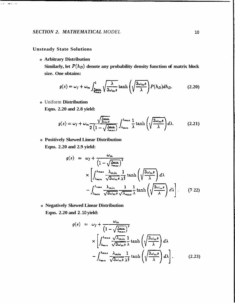
Unsteady State Solutions
0 Arbitrary Distribution Similarly, let P ( ~ D ) denote any probability density function of matrix block size. One obtains:
0 Uniform Distribution Eqns. 2.20 and 2.8 yield:
0 Positively Skewed Linear Distribution Eqns. 2.20 and 2.9 yield:
0 Negatively Skewed Linear Distribution Eqns. 2.20 and 2.10 yield:
(2.20)
(2.21)
22)
(2.23)
SECTION 2. MATHEMATICAL MODEL 11
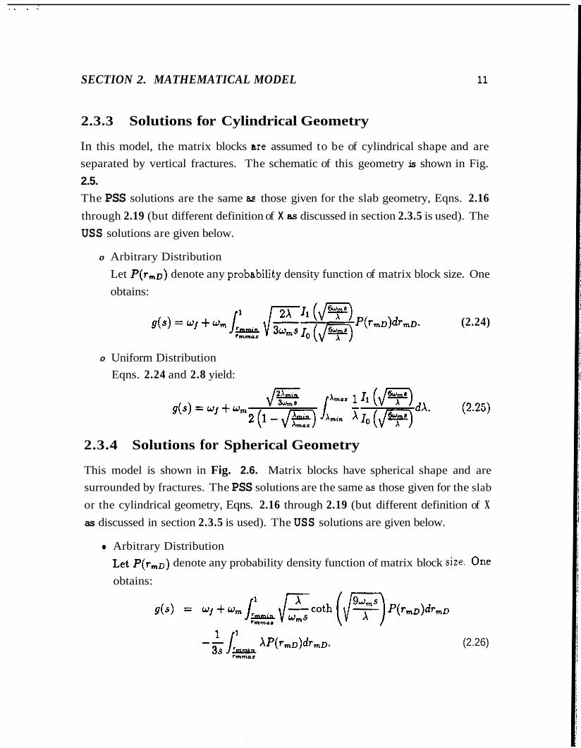
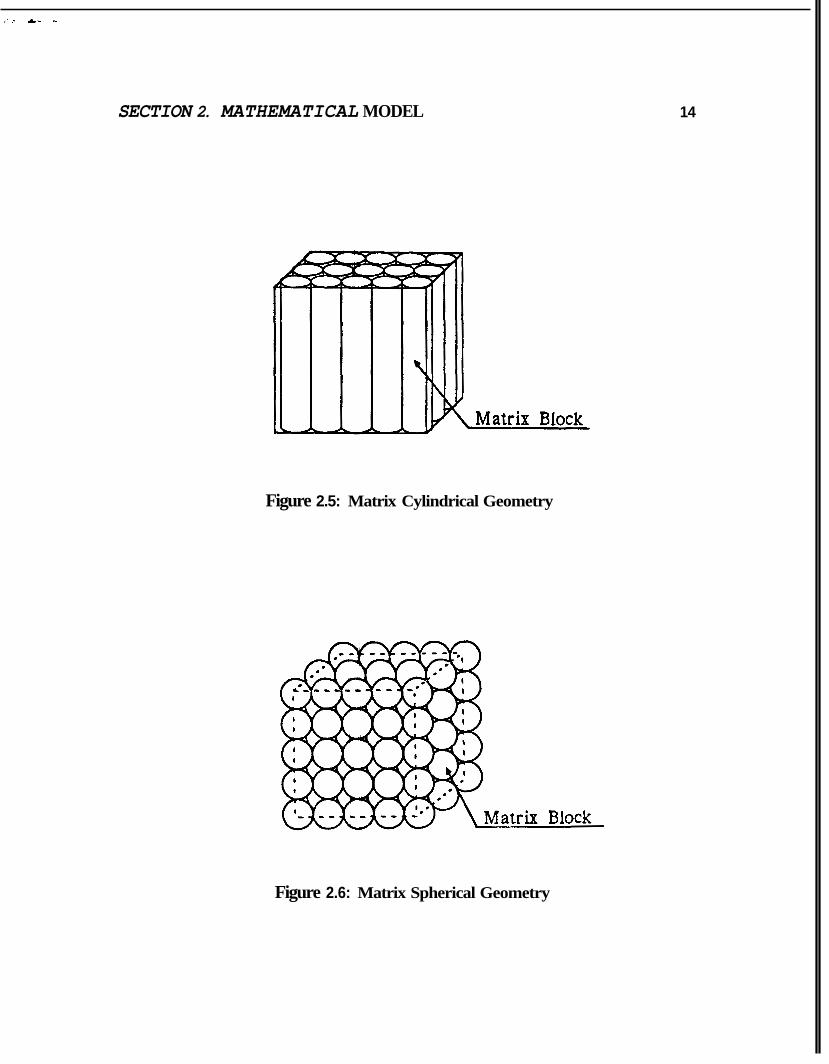
2.3.3 Solutions for Cylindrical Geometry
In this model, the matrix blocks are assumed to be of cylindrical shape and are separated by vertical fractures. The schematic of this geometry is shown in Fig. 2.5. The PSS solutions are the same as those given for the slab geometry, Eqns. 2.16 through 2.19 (but different definition of X as discussed in section 2.3.5 is used). The USS solutions are given below.
0 Arbitrary Distribution Let P(rfflD) denote any probability density function of matrix block size. One obtains:
(2.24)
0 Uniform Distribution Eqns. 2.24 and 2.8 yield:
2.3.4 Solutions for Spherical Geometry
This model is shown in Fig. 2.6. Matrix blocks have spherical shape and are surrounded by fractures. The PSS solutions are the same as those given for the slab
or the cylindrical geometry, Eqns. 2.16 through 2.19 (but different definition of X as discussed in section 2.3.5 is used). The USS solutions are given below.
0 Arbitrary Distribution Let P(r,o) denote any probability density function of matrix block size. One
obtains:
(2.26)
SECTION 2. MATHEMATICAL MODEL
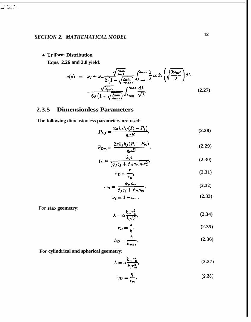
0 Uniform Distribution Eqns. 2.26 and 2.8 yield:
2.3.5 Dimensionless Parameters
The following dimensionless parameters are used:
For slab geometry:
For cylindrical and spherical geometry:
f7 f m
rlD = - 9
12
(2.27)
(2.28)
(2.29)
(2.30)
(2.31)
(2.32)
(2.33)
(2.34)
(2.35)
(2.36)
(2.37)
(2.3s)
SECTION 2. MATHEMATEA& MODEL 13
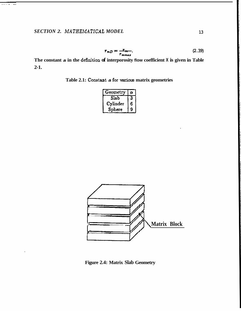
fmD = -. r m (2.39) rmmat
The constant a in the definition of interporosity flow coefficient X is given in Table 2-1.
Table 2.1: Constant a for various matrix geometries
?
r
? Matrix Block I
Figure 2.4: Matrix Slab Geometry
SECTION 2. MATHEMATICAL MODEL
Figure 2.5: Matrix Cylindrical Geometry
Figure 2.6: Matrix Spherical Geometry
14
Section 3
Discussion
In this work, flowrate and pressure response are considered and the factors which affect them are investigated. To convert the rate and pressure solutions from Laplace space into real space, Stehfest Algorithm (231 is used. The unsteady state solutions are evaluated using numerical integration.
3.1 Effect of Matrix Block Geometry
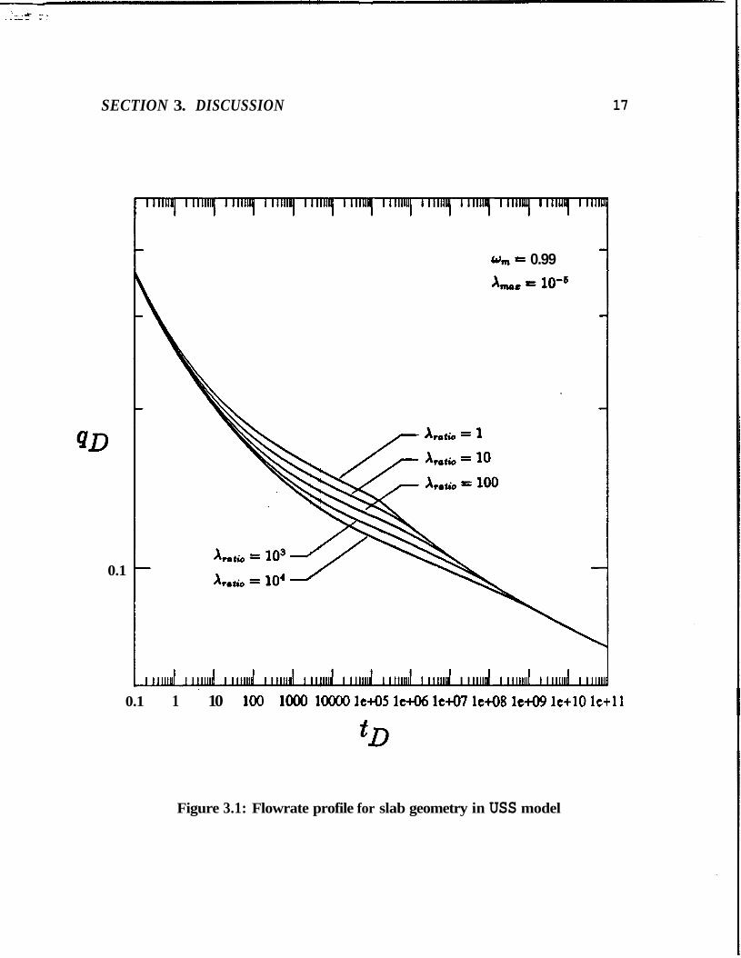
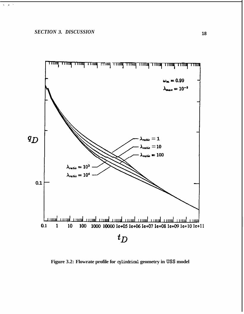
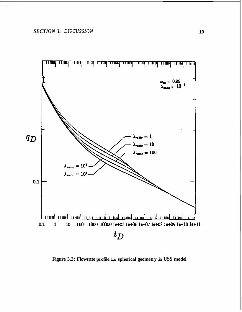
Figs. 3.1 through 3.3 show the rate response for the uniform distribution and USS interporosity flow for slab, cylindrical, and spherical matrix block geometries, respectively. Each figure is for m e value of wm and X,,,, and several values of Xralio.
The parameter Xratio is defined as:
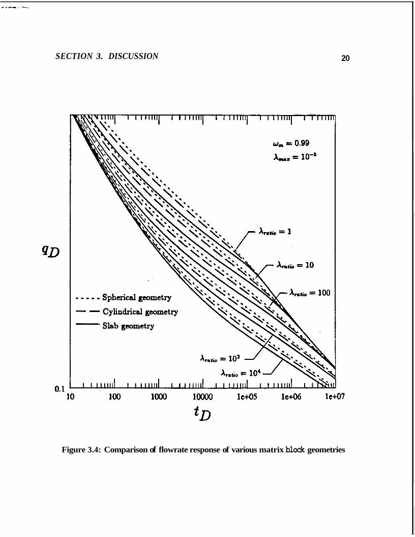
which is a measure of the spread (variance) of the matrix block size distribution and determines the duration of the interporosity flow period. In each of the Figs. 3.1 through 3.3, the interporosity flow period for a given Atatio begins and ends at the same time for the three geometries. This occurs because the duration of the interporosity flow period depends only on Xratio. The effect of block geometry appears only in the interporosity flow period. Fig. 3.4 shows that the spherical model yields a higher flowrate than the Cylindrical model, which in turn yields a
15
SECTION 3. DISCUSSION 16
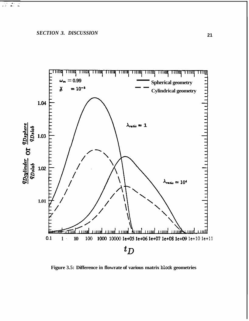
higher flowrate than the slab model. The differences are, however, not significant. Also, as Fig. 3.5 indicates, as X*atio increases, the difference in flowrate decreases.
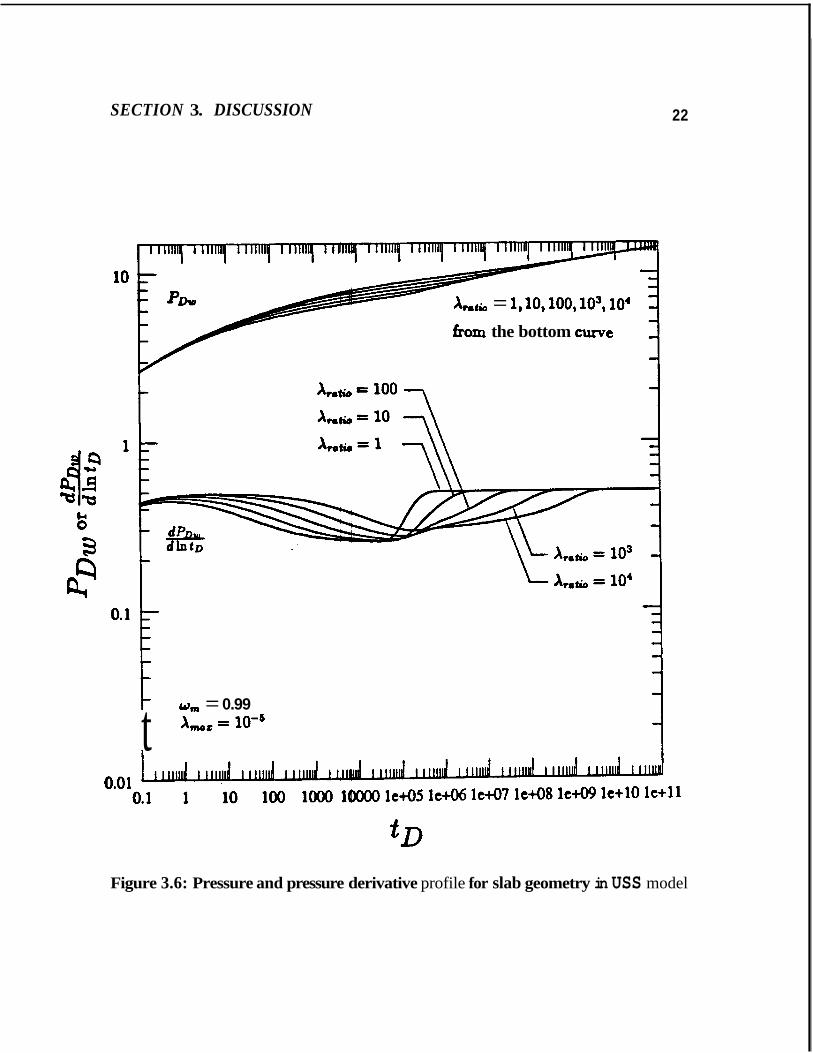
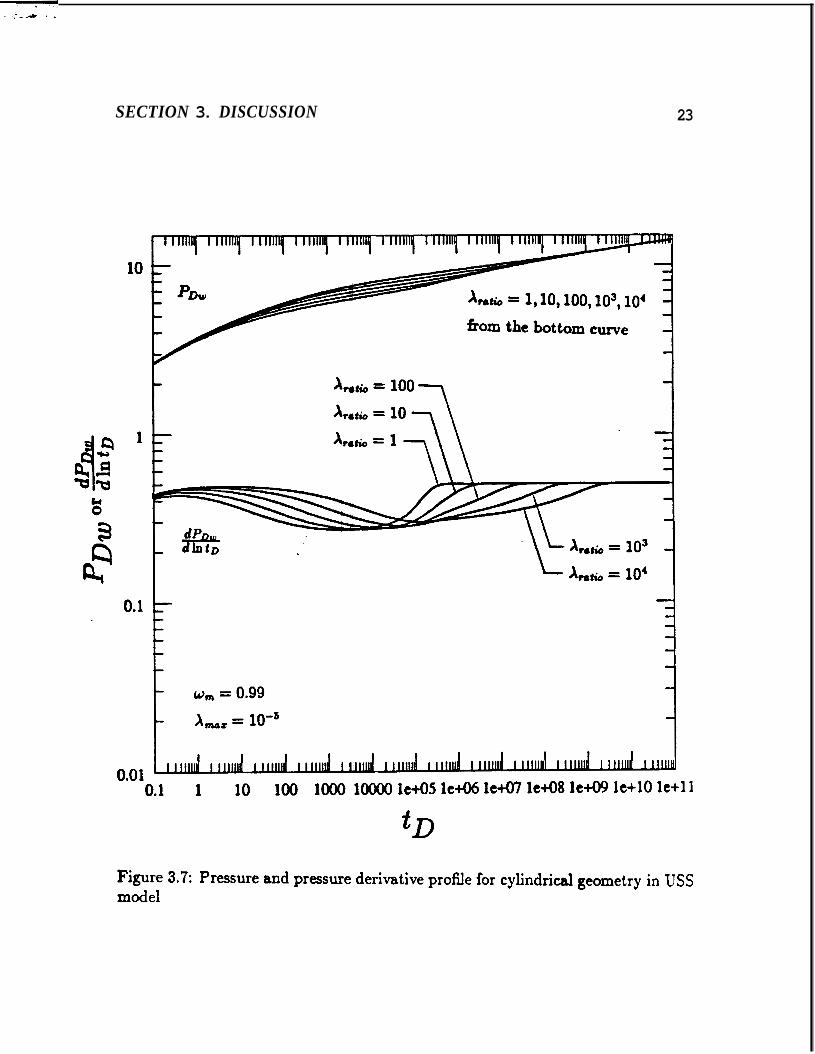
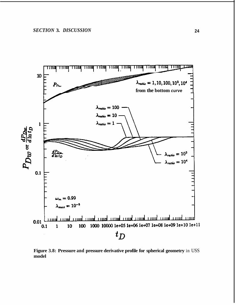
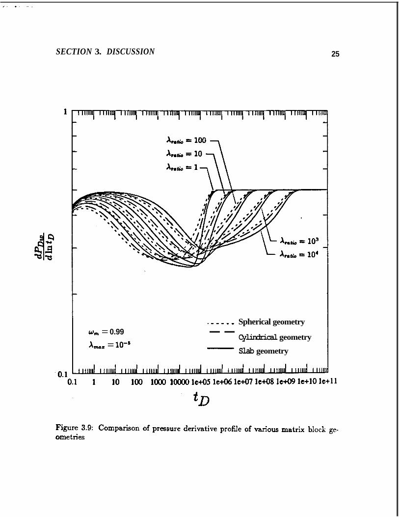
Figs. 3.6 through 3.8 show the pressure and the pressure derivative response for constant rate production for slab, cylindrical, and spherical geometries, respectively. Fig. 3.9 compares the pressure derivative response for the three geometries. The spherical model shows a smoother derivative profile than the cylindrical or the slab models, especially for small Xtafio. Due to the striking similarity of the rate and the pressure response for the three bbck geometries, only the slab model will be used for the remainder of this study.
SECTION 3. DISCUSSION 17
QD
0.1
0, = 0.99
0.1 1 10 100 lo00 10000 l e 4 5 let06 le+07 l e 4 8 let09 le+10 l t+ l l
Figure 3.1: Flowrate profile for slab geometry in USS model
i 4 -
SECTION 3. DISCUSSION
QD
0.1
i
18
-
\
I l l
- = 0.09
A m * = 10''
4 x,t, = 1
A,t, = 10
7 x,t, = 100
0.1 1 10 100 loo0 l o o 0 0 le+05 lt+06 le+07 l e 4 8 le+09 lt+10 k + l l
Figure 3.2: Flowrate profile for cylindrical geometry in USS model
SECTION 3. DXSCUSSION
QD
0.1
t Om = 0.99
19
1 I r l r l d I I
0.1 1 10 100 l o o 0 1~oooO le+O5 le+06 leI-07 l e 4 8 k+09 le+10 k + l l
Figure 3.3: Flowrate profile for spherical geometry in USS model
SECTION 3. DISCUSSION 20
100 l o o 0 0 le+05 le+06 l e 4 7
Figure 3.4: Comparison of flowrate response of various matrix block geometries
SECTION 3. DISCUSSION 21
1.02
1.01
w, = 0.99
x,, = 10'' - Spherical geometry -- Cylindrical geometry
xmtw = 1
0.1 1 10 100 lo00 l o o 0 0 l e 4 5 le+06 l e 4 7 l e 4 8 le+09 lt+10 let11
Figure 3.5: Difference in flowrate of various matrix block geometries
SECTION 3. DISCUSSION
10 s . ~ = 1, IO, loo, 103,104 &om the bottom curve
OS1 1 om = 0.99 t x,, = 10-5 1
22
tD Figure 3.6: Pressure and pressure derivative profile for slab geometry in USS model
SECTION 3. DISCUSSION 23
SECTION 3. DISCUSSION 24
10
from the bottom curve
Figure 3.8: Pressure and pressure derivative profile for spherical geometry in USS model
r i .: - .
SECTION 3. DISCUSSION 25
o m = 0.99
Am+ = lo-6
.---.I- Spherical geometry -- Cylindrical geometry
Slab geometry
SECTION 3. DISCUSSION 26
3.2 Effect of the Mode of Interporosity Flow
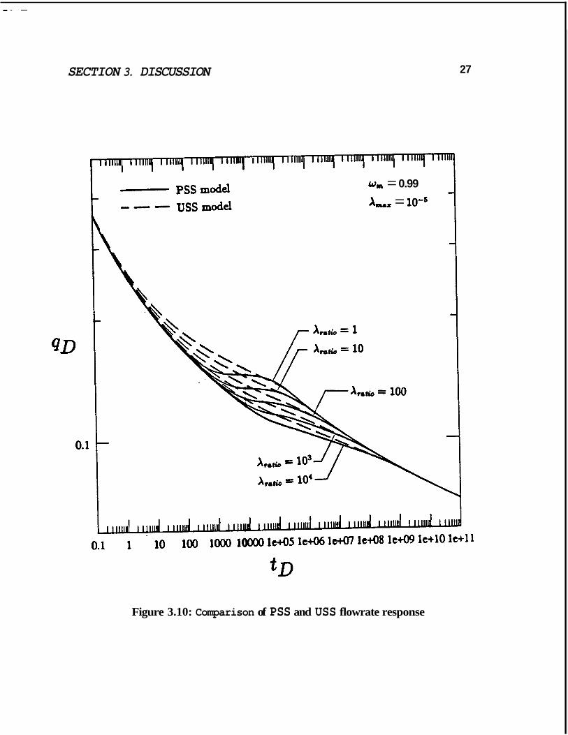
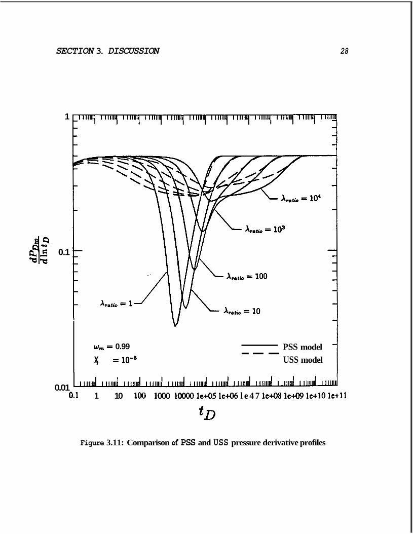
Fig. 3.10 is a flowrate profile that compares the USS and PSS response for several values of Xrotio. The interporosity flow period ends at the same time for these two models, however, the beginning time is different. In the USS model, the interporos- ity flow period begins much earlier than in the PSS model. Thus, the duration of the interporosity flow period of the USS model is much longer than that of the PSS model. Also, the USS model yields a higher flowrate than the PSS model during the interporosity flow period. Both models produce at exactly the same flowrate at the end of this period. Thus, the USS model yields a larger cumulative produc- tion. In the PSS model, the flowrate during the interporosity flow period is almost constant for small Xrotio values. In the USS model, on the other hand, a period of constant flowrate does not occur and a gradual decline is observed throughout the interporosity flow period. This gradual flowrate decline is particularly pronounced for large Xroiio values. Fig. 3.11 shows the comparison of pressure derivative profiles for the PSS and the USS models. The figure shows the sharp character of the PSS profile compared to the USS profile.
. . - - -
SECTION 3. DISCUSSION
QD
0.1
I I l l
WAI = 0.99
A- = 10’’
\.
27
Figure 3.10: Comparison of PSS and USS flowrate response
SECTION 3. DISCUSSION 28
1
dz 0.1 'tt'tf
0.01
Y
w, = 0.99
x,,, = 10-5
1 PSS model USS model --- 1
0.1 1 10 100 lo00 loo00 l e 4 5 le& l e 4 7 let08 le+09 le+10 le+ll
Figure 3.11: Comparison Of PSS and USS pressure derivative profiles
SECTION 3. DlSCUSSION 29
3.3 Effect of PDF Type
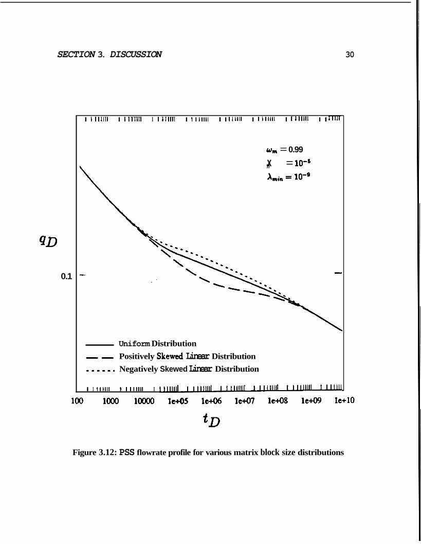
In this section, the rate and the pressure response for three matrix block size distri- butions - uniform, positively skewed linear, and negatively skewed linear distribu- tions, are examined. Both PSS and USS modes of interporosity flow are considered. Only the slab matrix geometry is used, since the transient response is not very sensitive to the matrix block geometry (see section 3.1).
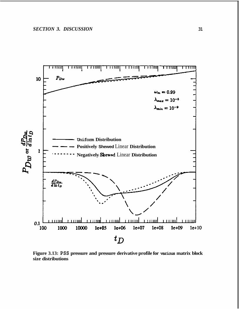
Fig. 3.12 shows the PSS flowrate profile for the three probability density func- tions. The duration of the interparosity flow period is the same for the three models. The probability distribution function does not affect the duration of this period as long as the limits of the distribution (Amin and X,,,) are the same. The response shows the lowest flowrate for the positively skewed linear distribution arld the high- est flowrate for the negatively skewed linear distribution. This indicates that the higher frequency of smaller matrix block sizes yields a higher flowrate. The flowrate for the uniform distribution is between that of the positively and the negatively skewed linear distributions, but is closer to the latter. This implies that the adverse effect of large blocks on reservoir producibility outweighs the advantage of small blacks. Fig. 3.13 shows the PSS pressure and the pressure derivative response for
the three distributions. The positively skewed distribution, which corresponds to a higher frequency of larger blocks, shows a delayed response.
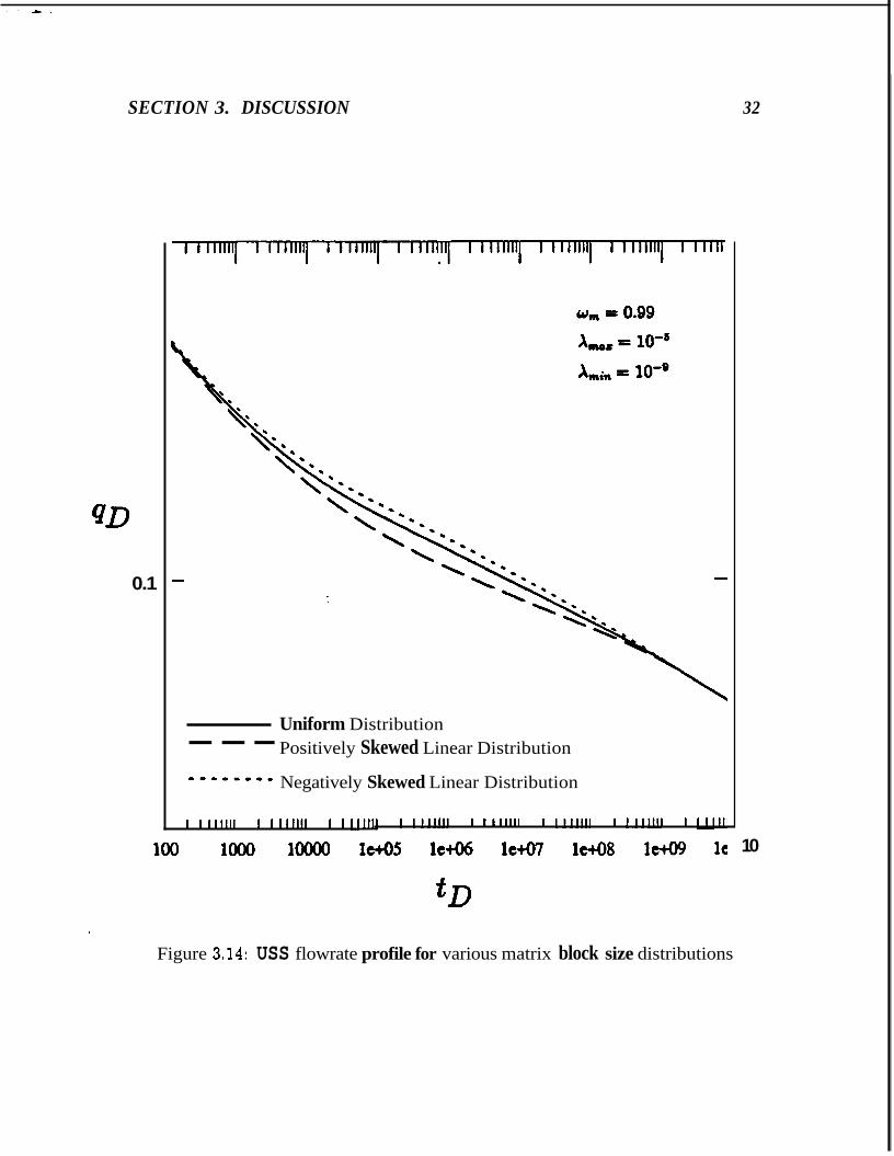
Figs. 3.14 and 3.15 show the rate profile and the pressure derivative profile for the USS model, respectively. The effect of the probability density function is less significant compared to the PSS model. However, the features which were mentioned with regard to the PSS model are observed here as well.
SECTION 3. DISCUSSION 30
QD
0.1
I 1 1 1 1 1 1 1 I I111111 I I111111 I I111111 I I llllll I 1 1 1 1 1 1 1 I I111111 I I lllrr
urn = 0.99
x,, = lo-&
Uniform Distribution - - Positively Skewad Linear Distribution ....-. Negatively Skewed Linear Distribution
I 1 I11111 I 1 1 1 1 1 1 1 I I U U
100 lo00 l o o 0 0 ltM5 le+O6 le+O7 le+O8 let09 k+10
tD
Figure 3.12: PSS flowrate profile for various matrix block size distributions
SECTION 3. DISCUSSION 31
P
0.
Uniform Distribution 1 Positively Shewed Linear Distribution
Negatively Skewed Linear Distribution
L'
Figure 3.13: PSS pressure and pressure derivative profile for various matrix block size distributions
. : * .
SECTION 3. DISCUSSION 32
QD
0.1
Uniform Distribution --- Positively Skewed Linear Distribution ---.--.- Negatively Skewed Linear Distribution
I I I 1 1 1 1 1 I I I11111 I 1 l U l I I111111 I 1 1 1 1 1 1 1 I I111111 I I 1 1 1 1 1 1 I I1111
100 1000 loo00 l&5 le+O6 lt+07 l e 4 8 le+09 le 10
Figure 3.14: USS flowrate profile for various matrix block size distributions
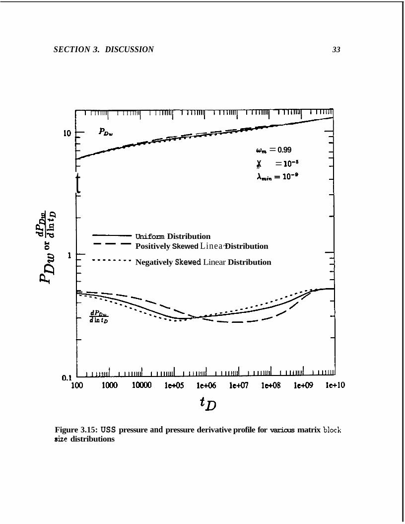
SECTION 3. DISCUSSION 33
I I 1 1 1 1 1 1 I I I I 11111 I I I rn
- - 0, = 0.99 - - - x,, = lo-6 -
t Uniform Distribution --- Positively Skewed Linea~ Distribution
0 - 0 - 0 0 0 0 Negatively Skewed Linear Distribution
100 lo00 l o o 0 0 lM5 l& le+07 1 ~ 0 8 le+09 1 ~ 1 0
Figure 3.15: USS pressure and pressure derivative profile for various matrix block rize distributions
SECTION 3. DISCUSSION 34
3.4 EEect of Fracture Intensity and Uniformity
Here, the effect of the mean and the variance of the matrix block size distribution on flowrate and cumulative recovery is considered. This is done for the uniform distribution and slab geometry for both PSS and USS models.
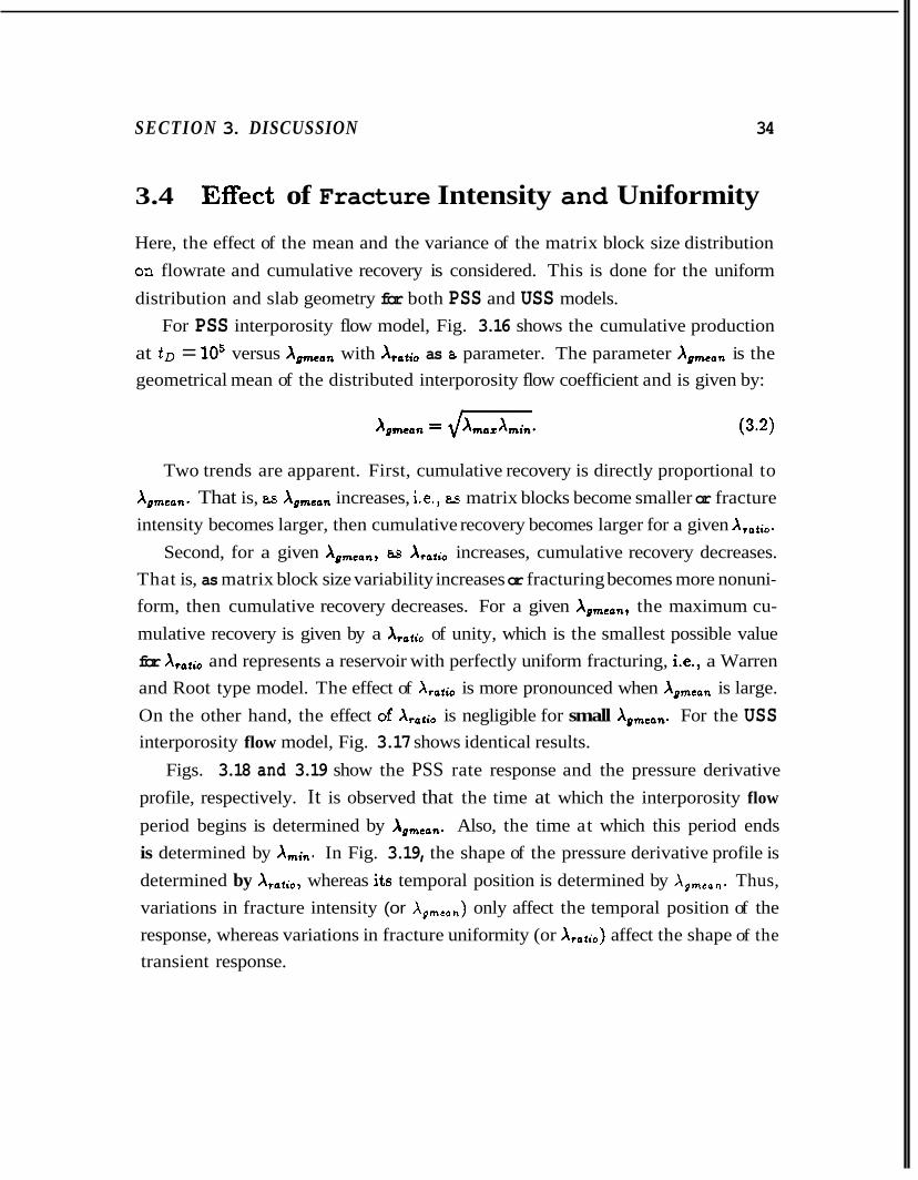
For PSS interporosity flow model, Fig. 3.16 shows the cumulative production at t~ = lo5 versus Xgmean with Xpatio as a parameter. The parameter Agmean is the geometrical mean of the distributed interporosity flow coefficient and is given by:
Two trends are apparent. First, cumulative recovery is directly proportional to Xgmean. That is, as Xgmean increases, ie., as matrix blocks become smaller or fracture intensity becomes larger, then cumulative recovery becomes larger for a given Xratio.
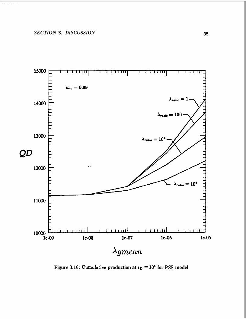
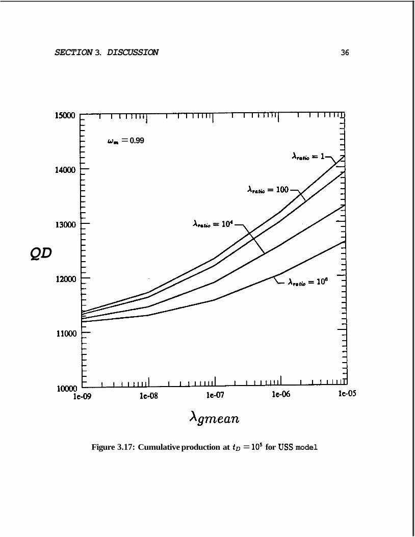
Second, for a given Anmean, &S X+atio increases, cumulative recovery decreases. That is, as matrix block size variability increases or fracturing becomes more nonuni- form, then cumulative recovery decreases. For a given Xgmcon, the maximum cu- mulative recovery is given by a Xrafio of unity, which is the smallest possible value for Xralio and represents a reservoir with perfectly uniform fracturing, Le., a Warren and Root type model. The effect of Xratio is more pronounced when Agmean is large. On the other hand, the effect ob Xratio is negligible for small Xgmean. For the USS interporosity flow model, Fig. 3.17 shows identical results.
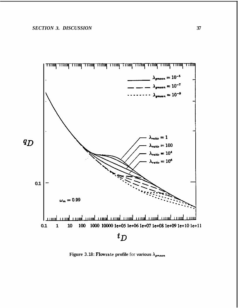
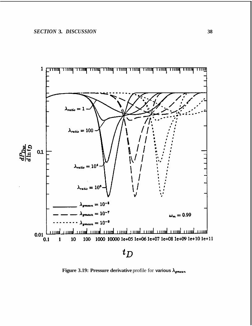
Figs. 3.18 and 3.19 show the PSS rate response and the pressure derivative profile, respectively. It is observed that the time at which the interporosity flow
period begins is determined by Agmean. Also, the time at which this period ends is determined by Amin. In Fig. 3.19, the shape of the pressure derivative profile is determined by Xratio, whereas its temporal position is determined by Xgmean. Thus, variations in fracture intensity (or Xgmean) only affect the temporal position of the response, whereas variations in fracture uniformity (or Xral io) affect the shape of the transient response.
QD
SECTION 3. DISCUSSION 35
Xgmean
Figure 3.16: Cumulative production at fD = IO5 for Pss model
SECTION 3. DISCUSSION 36
QD
E Wm = 0.99
Xgmean
Figure 3.17: Cumulative production at fD = lo5 for USS model
SECTION 3. DISCUSSION 37
QD
0.1
0.1 1 10 100 l o o 0 l o o 0 0 lc+O5 le& l e W le48 leM9 le+10 le+ll
t D
Figure 3.18: Flowraie profile for various A,,mean
SECTION 3. DISCUSSION 38
0.1
Figure 3.19: Pressure derivative profile for various X w a n
Section 4
Conclusion
1. The distributed formulation of interporosity flow predicts a gradual decline of the flowrate unlike the classical double porosity models which predict a sudden rate decline followed by a period of constant flowrate. This gradualness is more pronounced for larger matrix block size variabilities, i.e., cases of extremely nonuniform fracturing. Also, the gradualness is more apparent in the unsteady state model of interporosity flow.
2. Matrix block geometry does not have a significant effect on the rate or the pressure response. Spherical geometry yields slightly higher flowrate than the cylindrical geometry. The latter yields slightly higher flowrate than the slab geometry. Matrix block geometry only enters the formulation for unsteady state interporosity flow and not for pseudo-steady state interporosity flow.
3. The unsteady state formulation of interporosity flow yields higher flowrate (and hence higher cumulative recovery) than the pseudo-steady state formu- lation.
4. The negatively skewed linear distribution of matrix block size yields higher flowrate than the uniform distribution. The latter , in turn, yields higher flowrate than the positively skewed linear distribution. Thus, from the view- point of reservoi- producibility, it is more advantageous to have a high fre-
quency of small blocks than large blocks.
39

SECTION 4. CONCLUSION 40
5. Reservoir producibility is directly proportional to fracture intensity and in- versely proportional to the degree of fracture nonuniformity. Hence, the War- ren and Root model which assumes perfectly uniform fracturing, yields an upper bound of reservoir ptoducibility.
Nomenclature
A =
Cf =
area of matrix fracture interface, ft2
constant constant constant formation volume factor, RB/STB
constant constant constant fracture total compressibility, psi”
matrix total Compressibility, psi-’
wellbore storage coefficient, dimensionless
constant constant constant constant constant constant constant a parameter in the Bessel function argument
matrix block size for slab geometry, ft
matrix block size for slab geometry, dimensionless
41
NOMENCLATURE 42
maximum matrix block size, ft
minimum matrix block size, ft
modified Bessel function, first kind, zero order
modified Bessel function, first kind, first order
fracture permeability, md
matrix permeability, md
modified Beasel function, second kind, zero order
modified Bessel function, second kind, first order
fracture pressure, dimensionless
Laplace transfoamed fracture pressure
matrix pressure, dimensionless
Laplace transformed matrix pressure
wellbore pressure response, dimensionless
Laplace h-ansfotrmed wellbore pressure response
fracture fluid pressure, psi
probability density function of matrix block size distribution
probability density function of normalized matrix block size distribution in slab geometry
probability density function of normalized matrix block size distribution in cylindrical and spherical geometries
initial pressure, psi
matrix fluid pressure, psi
wellbore pressure response, psi
volumetric flow rate, STB/D
volumetric flow mte, dimensionless
Laplace transformed flow rate
cumulative production, dimensionless
NOMENCLATURE 43
Laplace transformed cumulative production
radial coordinate, ft
radial Coordinate, dimensionless
matrix block radius for cylindrical and spherical geometries, ft
matrix block radius for cylindrical and spherical geometries, dimensionless maximum matrix block radius, ft
minimum matrix block radius, ft
wellbore radius, ft
Laplace parameter
skin factor, dimensionless
time, hour
time, dimensionless
production time, dimensionless
interporosity flow contribution from matrix size h interporosity flow contribution from dimensionless matrix size
hD
interporosity flow contribution from dimensionless matrix ra- dius rmD
volume of matrix block, ft3
Bessel function argument
coordinate for dab matrix block dimensionless coordinate for slab matrix block constant in the definition of interporosity flow coefficient
coordinate for matrix block radius dimensionless coordinate for matrix block radius interporosity flow coefficient, dimensionless
NOMENCLATURE 44
Xgmeon geometrical mean of interporosity flow coefficient, dimension- less maximum interporosity flow coefficient, dimensionless
minimum interporosity flow coefficient, dimensionless
ratio of X,,, to Amin
viscosity, cp
fracture porosity, dimensionless
matrix porosity, dimensionless
fracture storativity ratio, dimensionless
matrix storativity ratio, dimensionless
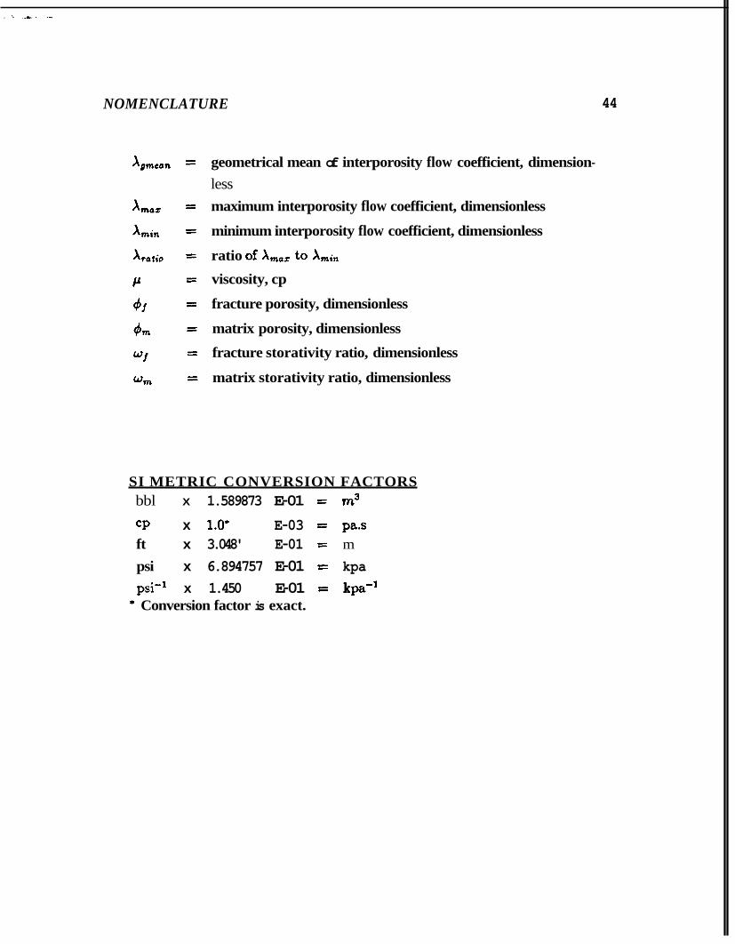
SI METRIC CONVERSION FACTORS bbl X 1.589873 E-01 = m3
C P x 1.0' E-03 = pas ft x 3.048' E-01 E m
psi x 6.894757 E-01 = kpa psi'' x 1.450 E-01 = kpa" ' Conversion factor is exact.
Bibliography
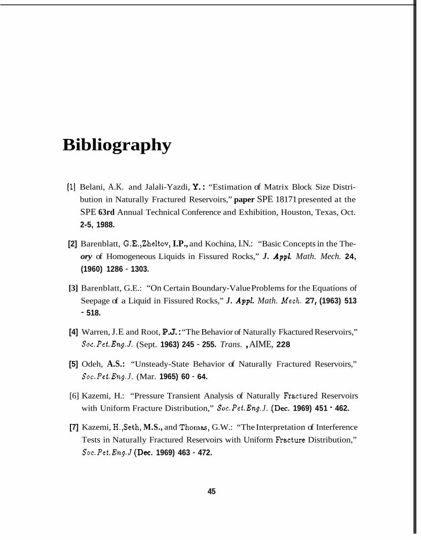
[l] Belani, A.K. and Jalali-Yazdi, Y.: “Estimation of Matrix Block Size Distri- bution in Naturally Fractured Reservoirs,” paper SPE 18171 presented at the SPE 63rd Annual Technical Conference and Exhibition, Houston, Texas, Oct. 2-5, 1988.
[2] Barenblatt, G.E.,Zheltov, I.P., and Kochina, I.N.: “Basic Concepts in the The- ory of Homogeneous Liquids in Fissured Rocks,” J. A p p l . Math. Mech. 24,
(1960) 1286 - 1303.
[3] Barenblatt, G.E.: “On Certain Boundary-Value Problems for the Equations of Seepage of a Liquid in Fissured Rocks,” J. A p p l . Math. Mech. 27, (1963) 513 - 518.
[4] Warren, J.E and Root, P.J.: “The Behavior of Naturally Fkactured Reservoirs,” S0c.Pet.Eng.J. (Sept. 1963) 245 - 255. Trans. , AIME, 228
[5] Odeh, A.S.: “Unsteady-State Behavior of Naturally Fractured Reservoirs,” Soc. Pet.Eng. J. (Mar. 1965) 60 - 64.
[6] Kazemi, H.: “Pressure Transient Analysis of Naturally Fkactured Reservoirs with Uniform Fracture Distribution,” Soc.Pet.Eng. J . (Dec. 1969) 451 - 462.
[7] Kazemi, H.,Seth, M.S., and Thomas, G.W.: “The Interpretation of Interference Tests in Naturally Fractured Reservoirs with Uniform Fkacture Distribution,” Soc.Pet. Eng.J (Dm. 1969) 463 - 472.
45
BIBLIOGRAPHY 46
[8) DeSwaan, O.A.: “Analytic Solution for Determining Naturally Fractured Reservoir Properties by Well Testing,” Soc.Pet.Eng. J. (June 1976) 117 - 122.
191 Najurieta, H.L.: “A Theory for Pressure Transient Analysis in Naturally Frac- tured Reservoirs,” J.Pet. Tech. (July 1980) 1241 - 1250.
[lo] Mavor, M.J. and Cinco-Ley, H.: “Transient Pressure Behavior of Naturally Fractured Reservoirs,” paper SPE 7977 presented at the SPE California Re- gional Meeting, Ventura, California, Apr. 18-20, 1979.
[ll] Kucuk, F. and Sawyer, W.K.: “Transient Flow in Naturally Fractured Reser- voirs and Its Application to Devonian Gas Shales,” paper SPE 9397 presented at the SPE 55th Annual Technical Conference and Exhibition, Dallas, Texas, Sept. 21-24, 1980.
[12] Deruyck, B.G., Bourdet, D.P., DaPrat, G., and h e y , H.J.Jr.: “Interpre- tation of Interference Tests in Reservoirs With Double Porosity Behavior - Theory and Field Ex.&nples,”’ paper SPE 11025 presented at the SPE 57th Annual Technical Conference and Exhibition, New Orleans, Louisiana, Sept. 26-29, 1982.
[13] Ohaeri, C.U.: “Pressure Buildup Analysis for a Well Produced at a Constant Pressure in a Naturally Fractured Reservoir;” paper SPE 12009 presented at the SPE 58th Annual Technical Conference and Exhibition, San Francisco, California, Oct. 5-8, 1983.
[14] Streltsova, T.D.: “Well Pressure Behavior of a Naturally Fractured Reservoir,” Soc. Pet.Eng. J . (Oct. 1983) 769 - 780.
[15] Cinco-Ley, H., Samaniego, F.V., and Kucuk, F.: “The Pressure Transient Be- havior for Naturally Fractured Reservoirs With Multiple Block Size,” paper SPE 14168 presented at the SPE 60th Annual Technical Conference and Ex- hibition, Las Vegas, Nevada, Sept. 22-25, 1985.
BIBLIOGRAPHY 47
[16] Jalali-Yazdi, Y. and Ershaghi, I.: “A Unified Type Curve Approach for Pres- sure Transient Analysis of Naturally Fractured Reservoirs,” paper SPE 16778 presented at the SPE 62nd Annual Technical Conference and Exhibition, Dal- las, Texas, Sept. 27-30,1987,
[17] DaPrat, G., Cinco-Ley, H., and Ramey, H.J.Jr.: “Decline Curve Analysis Using Type Curves for Two-Porosity System,” Soc. Pet. Eng. J . (June 1981) 354 - 362.
[18] Fetkovich, M.J.: “Decline Curve Analysis Using Type Curves,” J.Pet.Tech.
(June 1980) 1065 - 1077.
1191 Raghavan, R. and Ohaeri, C.U.: “Unsteady Flow to A Well Produced at Con- stant Pressure in a F’ractured Reservoir,” paper SPE 9902 presented at the SPE California Regional Meeting, Bakersfield, California, Mar. 25-26, 1981.
[20] Sageev, A., DaPrat, G., and Ramey, H.J.Jr.: “Decline Curve Analysis for Double-Porosity Systems,” paper SPE 13630 presented at the SPE California Regional Meeting, Bakersfield, California, Mar. 27-29, 1985.
[21] Jalali-Yazdi, Y., Belani, A.K., and Fujiwara, K.: “An Interporosity Flow Model for Naturally Fractured Reservoirs,” paper SPE 18749 presented at the SPE California Regional Meeting, Bakersfield, California, Apr. 5-7, 1989.
[22] van Everdingen, A.F. and Burst, W.: “The Application of the Laplace Trans- formation to Flow Problems in Reservoirs,” Trans. , AIME(1949), 186 305 - 324B.
[23] Stehfest, H.: “Algorithm 368, Numerical Inversion of Laplace Transforms,” Communications of the ACM D-5 (Jan. 1970) 13, No.1, 47 - 49.
Appendix A
Derivation of Solution
This appendix contains a derivation of the constant rate and constant pressure solutions.
A.1 Slab Geometry
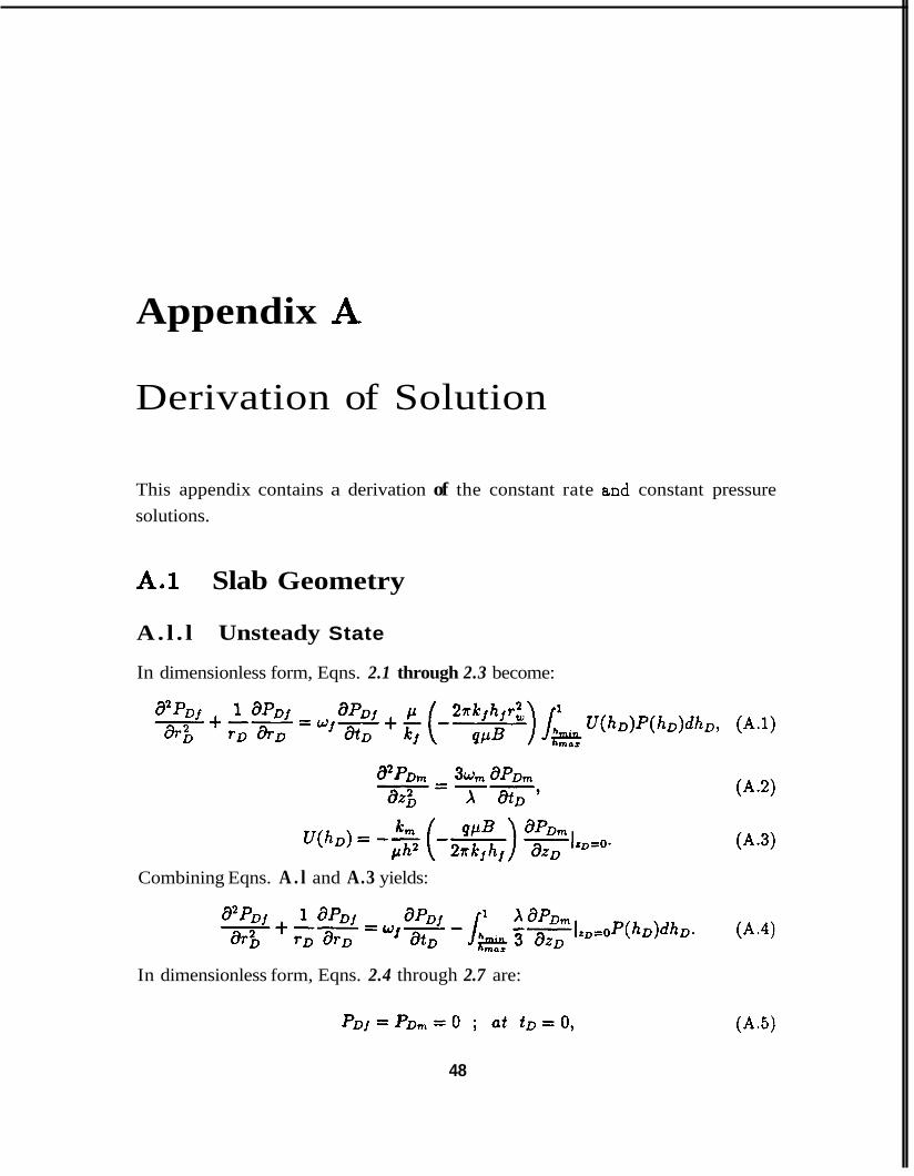
A. l . l Unsteady State
In dimensionless form, Eqns. 2.1 through 2.3 become:
Combining Eqns. A . l and A.3 yields:
In dimensionless form, Eqns. 2.4 through 2.7 are:
48
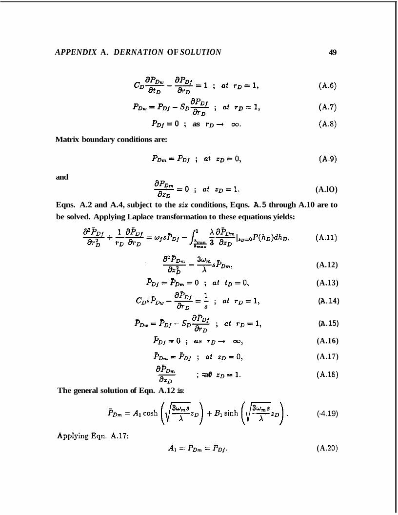
APPENDIX A. DERNATION OF SOLUTION 49
P D j = O ; as r D + 00.
Matrix boundary conditions are:
and (A.lO)
Eqns. A.2 and A.4, subject to the six conditions, Eqns. A.5 through A.10 are to be solved. Applying Laplace transformation to these equations yields:
a p D * - = 0 ; at . z D = ~ .
The general solution of Eqn. A.12 is:
(A.11)
(A.12)
(A.13)
(A.14)
(A.15)
(A.16)
(A.17)
(A.18)
(-4.19)
( A 2 0 )
APPENDIX A . DERNATION OF SOLUTION
Next, differentiating Eqn. A.19 and using Eqn. A.18:
Thus:
P D f
Substituting Eqn. A.22 into Eqn. A.l l , and rearranging yields:
where:
50
(A.21)
(A -22)
(A.23)
The general solution for Eqn. A.23 is:
Applying boundary condition, Eqn. A.16:
(A.25)
(A.26)
Differentiating Eqn. A.26:
From the skin and storage conditions, Eqns. A.14 and A.15: .
where:
(A 2 9 )
( A .30)
APPENDIX A . DERIVATION OF SOLUTION 51
The relation between flowrate and wellbore pressure in Laplace space is [22]:
1 SZPDW
ijD = -* (A.32)
Then, flowrate for no storage case is:
- XKl ( X ) q D =
8 {KO( 5 ) + s D x K l ( z ) } '
Cumulative production is given as:
(A.33)
(A.34)
A.1.2 Pseudo-Steady State
Solution for pseudo-steady state interporosity flow is obtained by eliminating the spacial dependency of time rate of change of pressure. That is, Eqn. A.2 becomes:
(A.35)
where & ( f D ) is independent of t ~ . This partial differential equation is solved as:
1 P D m 5E1(1D)zL -I- E ~ D + G I .
Applying boundary condition, Eqns. A.9, and A.lO:
Then:
(A.36)
(A.37)
G1 = Poi. (A .39)
APPENDIX A. DEWATION OF SOLUTION 52
By differentiating Eqn. A.40 and using Eqn. A.35:
(A .41)
Substituting Eqn. A.41 into Eqn. A.4, the diffusivity equation becomes:
In Eqn. A.40, by averaging &(to) across the matrix block thickness, the following equation is obtained:
(A .45)
Applying Laplace transfox&ation to Eqns. A.42 and A.45:
and
From Eqn. A.47:
Substituting Eqn. A.48 into Eqn. A.46, the following equation is obtained:
where:
(A .47)
(A .48)
(A.49)
(A .50)
Eqn. A.49 is the same as Eqn. A.23 in the unsteady state model, which yields the same general solution. The procedure and solutions of Eqns. A.25 through A.34 are valid for the pseudo-steady state model also.
APPENDIX A. DEWATION OF SOLUTION 53
A.2 Cylindrical Geometry
A.2.1 Unsteady State
In dimensionless form, Eqns. 2.1 through 2.3 become:
, - I
(A.52)
(A.53)
Combining Eqn. A.51 and Eqn. A.53 yields:
Eqns. A.5 through A.8 are used as initial and boundary conditions in cylindri- cal geometry, too. As for the boundary conditions for the matrix coordinate, the following are used instead of Eqns. A.9 and A.lO:
PDf ; at = 1, (A.55)
P D m is f inite at q D = 0. (A.56)
Applying Laplace transform to E q n s . A.54 and A.52:
and (A . 5S )
The boundary conditions in Laplace space are given by Eqns. A.13 through A.16 end the following two equations:
Pom i s f inite at VD = 0. -
(A.60)
APPENDIX A. DERIVATION OF SOLUTION
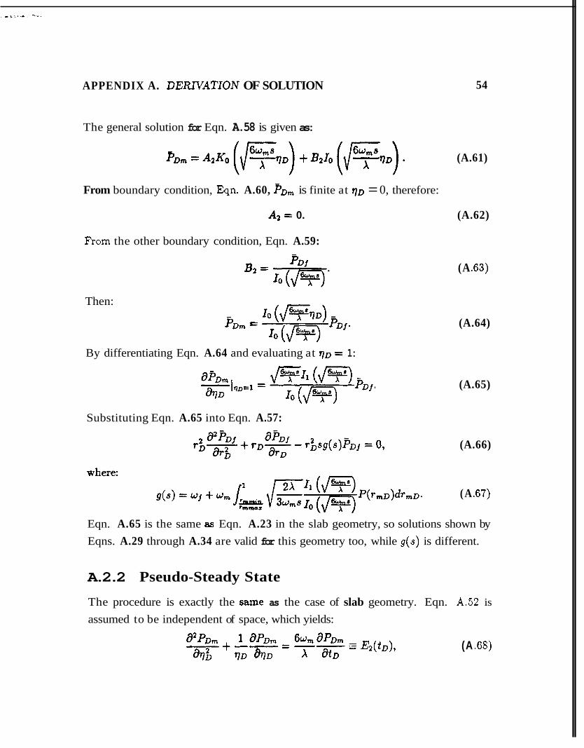
The general solution for Eqn. A.58 is given as:
From boundary condition, Eqn. A.60, PDm is finite at VD = 0, therefore:
A2 = 0.
F'rom the other boundary condition, Eqn. A.59: -
Then:
By differentiating Eqn. A.64 and evaluating at 70 = 1:
Substituting Eqn. A.65 into Eqn. A.57:
54
(A.61)
(A.62)
(A .63)
(A.64)
(A.65)
(A.66)
(A .67)
Eqn. A.65 is the same as Eqn. A.23 in the slab geometry, so solutions shown by Eqns. A.29 through A.34 are valid for this geometry too, while g(s) is different.
A.2.2 Pseudo-Steady State
The procedure is exactly the same as the case of slab geometry. Eqn. A.52 is
assumed to be independent of space, which yields:
(A .SS)
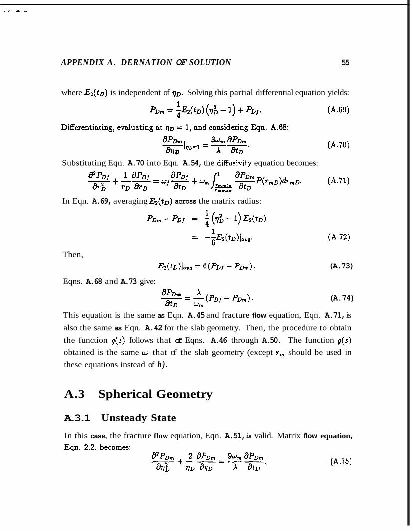
APPENDIX A . DERNATION OF SOLUTION 55
where & ( t D ) is independent of q ~ . Solving this partial differential equation yields:
Substituting Eqn. A.70 into Eqn. A.54, the diffusivity equation becomes:
In Eqn. A.69, averaging & ( t D ) across the matrix radius:
Then,
&(tD)lowg = 6 ( P D j - P D m ) - Eqns. A.68 and A.73 give:
(A.73)
(A.74)
This equation is the same as Eqn. A.45 and fracture flow equation, Eqn. A.71, is also the same as Eqn. A.42 for the slab geometry. Then, the procedure to obtain the function g(s) follows that of Eqns. A.46 through A.50. The function g(s)
obtained is the same as that of the slab geometry (except rm should be used in these equations instead of h) .
A.3 Spherical Geometry
A.3.1 Unsteady State
In this case, the fracture flow equation, Eqn. A.51, is valid. Matrix flow equation,
(A .75)
APPENDIX A. DERNATION OF SOLUTION
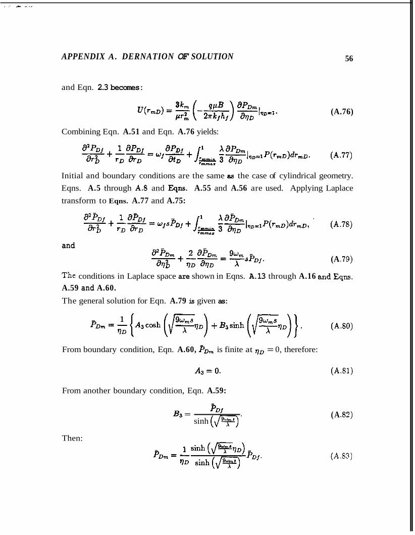
and Eqn. 2.3 becomes:
56
(A.76)
Combining Eqn. A.51 and Eqn. A.76 yields:
Initial and boundary conditions are the same as the case of cylindrical geometry. Eqns. A.5 through A.8 and Eqns. A.55 and A.56 are used. Applying Laplace transform to Eqns. A.77 and A.75:
and (A 3 9 )
The conditions in Laplace space are shown in Eqns. A.13 through A.16 and Eqm. A.59 and A.60. The general solution for Eqn. A.79 is given as:
From boundary condition, Eqn. A.60, p~~ is finite at = 0, therefore:
A3 = 0. (A.81)
From another boundary condition, Eqn. A.59:
P D j Bs = sinh (m *
Then:
(A .83)
(A.83)
APPENDIX A . DERNATION OF SOLUTION
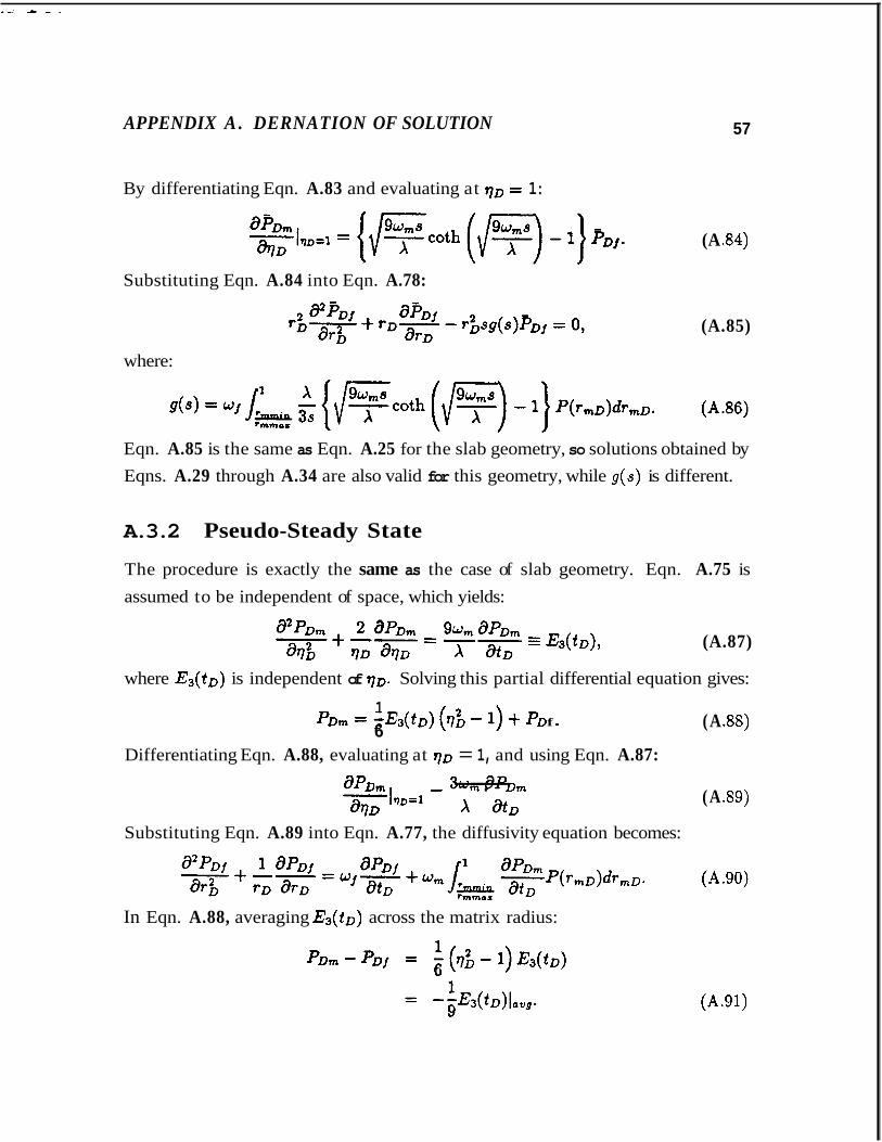
By differentiating Eqn. A.83 and evaluating at V D = 1:
Substituting Eqn. A.84 into Eqn. A.78:
57
(A .84)
(A.85)
where:
Eqn. A.85 is the same as Eqn. A.25 for the slab geometry, so solutions obtained by Eqns. A.29 through A.34 are also valid for this geometry, while g(s) is different.
A.3.2 Pseudo-Steady State
The procedure is exactly the same as the case of slab geometry. Eqn. A.75 is assumed to be independent of space, which yields:
(A.87)
where E 3 ( t D ) is independent of q ~ . Solving this partial differential equation gives:
1 6 porn = - & ( t o ) (7; - 1) + P D f (A 38)
Differentiating Eqn. A.88, evaluating at V D = 1, and using Eqn. A.87:
a P D m - - --. 3wrn a p D m -11)0=1 x a t D (A .S9) 3770
Substituting Eqn. A.89 into Eqn. A.77, the diffusivity equation becomes:
In Eqn. A.88, averaging & ( t ~ ) across the matrix radius:
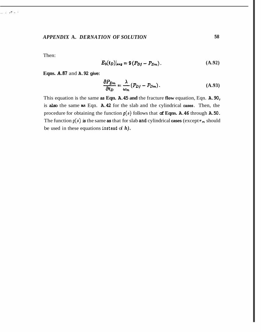
APPENDIX A. DERNATION OF SOLUTION 58
Then:
& ( f ~ ) l o v g = 9 ( P D ~ - porn).
Eqns. A.87 and A.92 give:
(A.92)
(A.93)
This equation is the same as Eqn. A.45 and the fracture flow equation, Eqn. A.90, is also the same 8s Eqn. A.42 for the slab and the cylindrical cases. Then, the procedure for obtaining the function g(s) follows that of Eqns. A.46 through A.50. The function g(s) is the same as that for slab and cylindrical cases (except r, should be used in these equations instead of h).
Appendix B
Computer Programs
This section contains the computer programs which are used in this study. To solve
some of the equations, IMSL fortran routines were used.
59
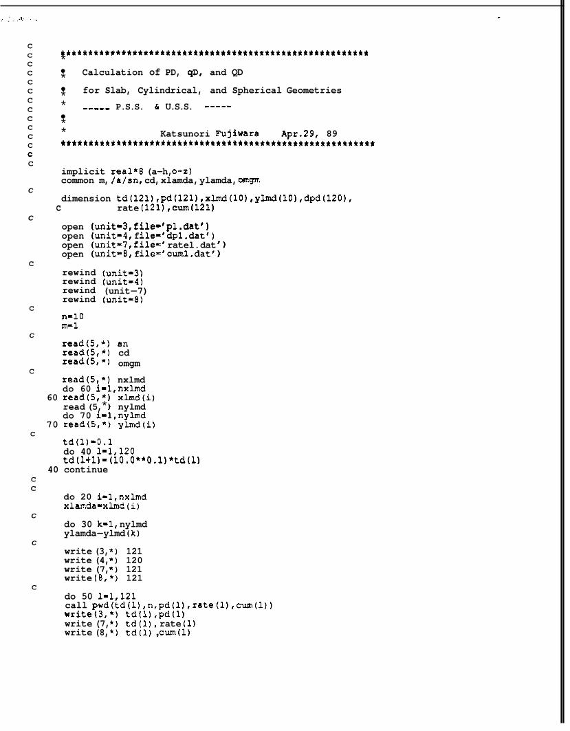
C C C C C C C C C C C C
. . . . . . . . . . . . . . . . . . . . . . . . . . . . . . . . . . . . . . . . . . . . . . . . . . . . . . . .
Calculation of PD, qD, and QD
for Slab, Cylindrical, and Spherical Geometries
* ----- P.S.S. c U.S.S. -----
* * *
* * Katsunori Pujiwara Apr.29, 89 . . . . . . . . . . . . . . . . . . . . . . . . . . . . . . . . . . . . . . . . . . . . . . . . . . . . . . . . .
C implicit real*8 (a-h, 0 - 2 ) common m, /a/sn, cd, xlamda, ylamda, mgm
dimension td(121) ,pd(121) ,xlmd(lO) ,ylmd(lO) ,dpd(l20), C
c rate (121) ,cum(l21) C
open (unit=3,file='pl.datt) open (unit=4, f ile='dpl .dat' ) open (unit=7, file-' ratel. dat open (unit=8, f ile-'cuml .dat'
rewind (unit=3) rewind (unit=4) rewind (unit-7) rewind (unit=8)
n=lO m-1
read(5, *) sn read(5, *) cd read(5, *) omgm
read(5, *) nxlmd do 60 i=l,nxlmd
read (5, * nylmd do 70 i=l,nylmd
C
C
C
C
60 read(5,*) xlmd(i)
70 read(5,*) ylmd(i) C
td(1)-0.1 do 40 1=1,120 td(l+l)-(lO.O**O.l)*td(l)
40 continue C C
do 20 i=l,nxlmd xlamdatxlmd (i)
do 30 kel, nylmd ylamda-ylmd (k)
write (3, * ) 121 write (4, *) 120 write (7, * ) 121 write (B, * ) 121
C
C
C do 50 1-1,121 call pwd(td(1) ,n,pd(l) ,rate(l) ,cum(l)) write(3,*) td(1) ,pd(l) write (7, *) td(l), rate (1) write (8, *) td(1) , cum(1)
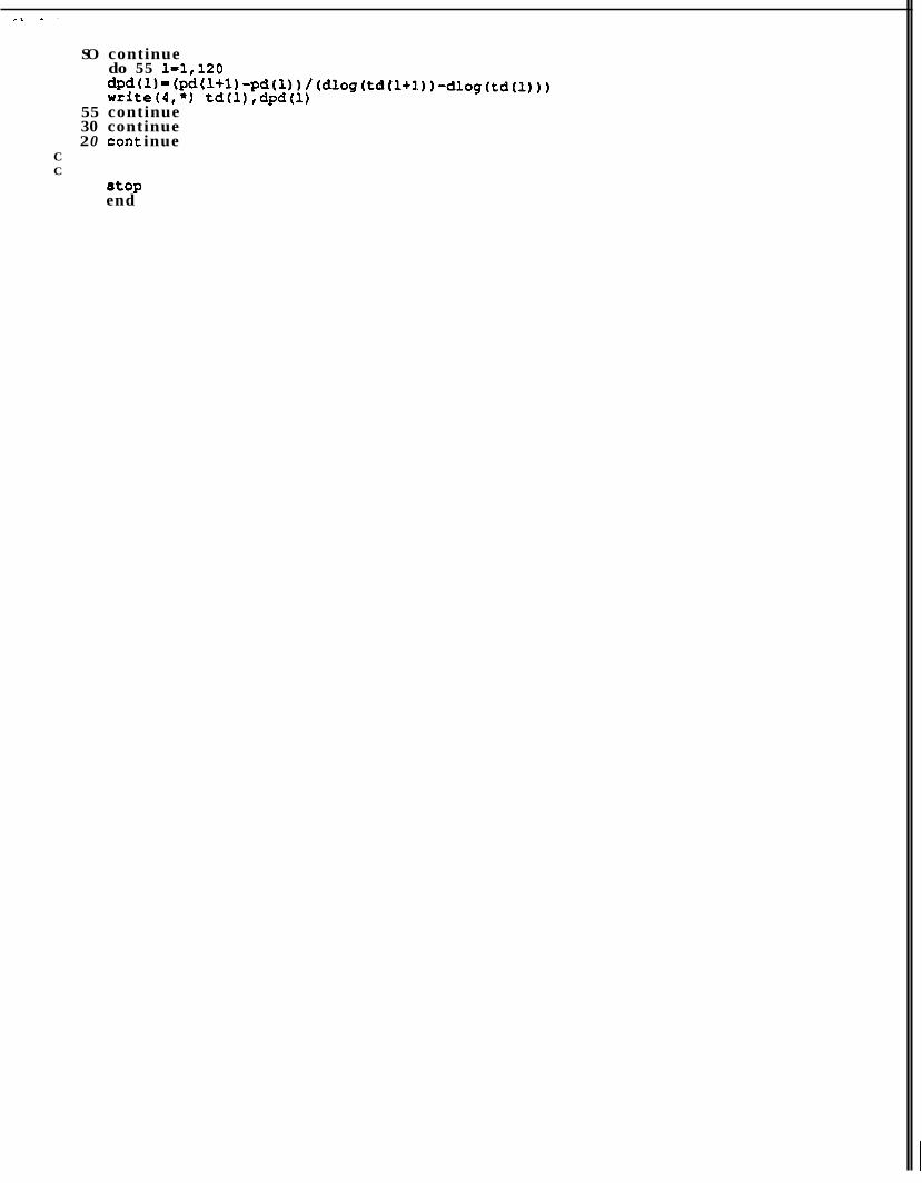
SO continue do 55 111,120 dpd(l)=(pd(l+l)-pd(l))/(dl~g(td(l+l.))-dlog(td(l))) write(4, *) t d ( 1 ) ,dpd(l)
55 continue 30 continue 2 0 cont inue
C C
stop end
* L * - I .- .A.
'.C C C C C C c 'C C C C C C C
C C
C
C
C C
C
C
. . . . . . . . . . . . . . . . . . . . . . . . . . . . . . . . . . . . . . . . . . . . . . . . . . . . . . . . * * Calculation of PD,qD, and OD
for Slab, Cylindrical, and Spherical Geometries
* --_-- * P . S . S . ----- * Katsunori Fujiwara Apr.29, 89 . . . . . . . . . . . . . . . . . . . . . . . . . . . . . . . . . . . . . . . . . . . . . . . . . . . . . . . . .
function plapl(s) implicit real*8 (a-h,o-z) double precision kO,kl,gg,xx common m,/a/sn,cd,xlamda,ylamda,omgm
if (xlamda .eq. ylamda) then gg-1.0-omgm+omgm*xlamda/(omgm*s+xlamda) else gg=l. 0-omgm+omgm*dsqrt (xlamda/omgm/s) / (1.0-
& dsqrt (xlamda/ylamda) ) * C (datan (dsqrt (ylamda/omgm/s) 1 -Batan (sqrt (xlamda/omgm/ & SI)) endif
xx=dsqrt (s*gg) k0-dbsk0 (xx) kl-dbskl ( x x ) PlaPl= (kO+sn*xx*kl) / (s* (cd*s* (kO+sn*xx*kl) +xx*kl) ) return end
function plap2 (5) implicit real*8 (a-h, 0 -2 ) double precision kO, kl, gg, plap, xx Cornon m, /a/sn, cd, xlamda, ylamda, omgm
if(x1amda .eq. ylamda) then gg-1.0-omgm+omgm*xlamda/(omgm*s+xlamda) else gg=1 .O-omgm+omgm*dsqrt (xlamda/omgm/s) / (1.0-
C dsqrt (xlamda/ylamda) ) * C (datan (dsqrt (ylamda/omgm/s) ) -ciatan (sqrt (xlamda/omgm/ & SI)) endif
xx=dsqrt (s*gg) kO-dbskO (xx) kl-dbskl (xx) plap=(kO+sn*xx*kl)/(s*(cd*s*(kO+~n*xx*kl)+xx*kl)) plap2=l./s/s/plap return end
function plap3 (s) implicit raal*8 (a-h, 0 - 2 ) double precision kO, kl,gg,plap,xx
cornon m, /a/sn, cd, xlamda,ylamda, omgm C .C
if (xlamda .eq. ylamda) then gg=l.O-omgm+omgm*xlamda/ (omgm*s+xLamda) else gg=l.O-omgm+omgm*dsqrt(xlamda/om~/s)/(l.O-
& dsqrt (xlamda/ylamda) ) c (datan (dsqrt (ylamda/omgm/s) 1 -&tan (sqrt (xlamda/omgm/ c SI)) endi f
ur-dsqrt (s*gg) kO-dbskO ( x x ) kl-dbskl (xx) plap- (kO+sn*xx*kl) / (s* (cd*s* (kO+sn*xx*kl) +xx*kl) ) plap3=l./s/s/s/plap return end
. .a-
C C C C C C C C C C C C
C C
C
C C
C C
C
. . . . . . . . . . . . . . . . . . . . . . . . . . . . . . . . . . . . . . . . . . . . . . . . . . . . . . . . *
Calculation of PD,qD, and OD
* for Slab Geometry ----- U . S . S . ----- * * t * Katsunori Pujiwara . . . . . . . . . . . . . . . . . . . . . . . . . . . . . . . . . . . . . . . . . . . . . . . . . . . . . . . . .
function plapl(s,ans) implicit real*6 (a-h, 0 -2 ) double precision kO, kl,gg, xx comon m, /a/sn, cd, xlamda, ylamda, mgm
if (xlamda .ne. ylamda) then
& dsqrt (xlamda/ylamda) ) *ans gg-1.0-omgm+omgm*dsqrt (xlamda/3. Jomgm/s) / (1 .O-
else gg-1. 0-omgm+omgm*dsqrt (xlamda/3. Jomgm/s) *
C dtanh (dsqrt (3. *omgm*s/xlamda) ) endif
ut-dsqrt (s*gg) kO-dbskO (xx) kl-dbskl (xx) plapl= (kO+sn*xx*kl) / (s* (cd*s* (kO+sn*xx*kl) +xx*kl) ) return end
function plap2 (5, ans) implicit real*8 (a-h, 0-2) double precision kO,kl,gg,plap,xx common m, /a/sn, cd, xlamda, ylamda, oangm
if (xlamda .ne. ylamda) then
6 dsqrt(xlamda/ylamda))*ans ggll.0-omgmiomgm*dsqrt (xlamda/3./omgm/s) / (1.0-
else gg=l.0-omgmiomgm*dsqrt(xlamda/3./omgm/s)*
C dtanh(dsqrt(3.*omgm*s/xlamda)) endif
xx-dsqrt (s*gg) kO-dbsk0 (xx) kl-dbskl (xx) plapt (kO+sn*xx*kl) / (s* (cd*s* (kO+sn*xx*kl) +xx*kl) ) plap2=l./s/s/plap return end
function plap3 (s,ans) implicit real*8 (a-h, 0 -2 ) double precision kO, kl, gg, plap, xx common m, /a/sn, cd, xlamda, ylamda, omgm
C C
. . .. .. - _.. .
if (xlamda .ne. ylamda) then
C dsqrt (xlamda/ylamda) ) *ans gg=l. 0-omgm+omgm*dsqrt (xlamda/3. /omgm/s) / (1.0-
gp1.O-omgm+omgm*dsqrt (xlamda/3. /omgm/s) * else
C dtanh (dsqrt ( 3 . *omgm*s/xlamda) ) endif
ut-dsqrt (s*gg) k0-dbsk0 ( x x ) kl=dbskl (xx) p l a p (kO+sn*xx*kl) / (s* (cd*s* (kOtsn*xx*kl) +xx*kl) ) plap3=1./s/s/s/plap return end
C
C Definition of function f which is used for integration
function f (x) implicit real*8 (a-h, 0 - 2 )
fldtanh (x) /x return end
C
. . .. 2.
C C C C C C C C C C C C
C C
C
C C
C C
C
C C
C C
. . . . . . . . . . . . . . . . . . . . . . . . . . . . . . . . . . . . . . . . . . . . . . . . . . . . . . . . * Calculation of PD,qD, and OD
* for Cylindrical Geometry --*-- * Katsunori Fujiwara
. . . . . . . . . . . . . . . . . . . . . . . . . . . . . . . . . . . .
U . S . S .
******* **
function plapl(s,ans) implicit real*8 (a-h, 0 - 2 ) double precision kO I kl, gg, xx common m, /a/sn, cd, xlamda, ylamda, omgm
if(x1amda .ne.ylamda) then gg-l.0-omgm+omgm*dsqrt(2.*xlamda/3./omgm/s)/(l.O-
& dsqrt (xlamda/ylamda) ) *ans else gg-1.0-omgm+omgm*dsqrt (2. *xlamda/3. /omgm/s) *
& dbsile(dsqrt(6.*omgm*s/xlamda~)/ & dbsiOe(dsqrt(6.*omgm*s/xlamdal) endif
xxrdsqrt (s*gg) k0-dbsk0 ( x x ) kl-dbskl ( x x ) plapl= (kO+sn*xx*kl) / (s* (cd*s* (kO+sn*xx*kl) +xx*kl) ) return end
function plap2 (5, ans ) implicit real*8 (a-h, 0-2) double precision kO I kl, gg, xx common m, /a/sn, cd, xlamda, ylamda, omgm
if(x1amda .ne.ylamda) then gg=1 .O-omgm+omgm*dsqrt (2. *xlamda/3. /omgm/s) / (1.0-
& dsqrt (xlamda/ylamda) ) *ans else gg=l.0-omgm+omgm*dsqrt(2.*xlamda/3./omgm/s)*
& dbsile(dsqrt(6.*omgm*s/xlamda))/ L dbsiOe (dsqrt (6. *omgm*s/xlamda) ) endif
aucldsqrt (s*gg) k0-dbsk0 (xx) kltdbskl (xx) plap- (kOtsn*xx*kl) / (s* (cd*s* (kO+sn*xx*kl) +xx*kl) ) plap2=l./s/s/plap return end
function plap3 (3, ans) implicit real*8 (a-h, 0 - z ) double precision kO, kl, gg, xx common m, /a/sn, cd, xlamda, ylamda,omgm
**** **
if(x1amda .ne.ylamda) then
gg-1.0-omgm+omgm*dsqrt (2. *xlamda/3. /omgm/s) / (1.0- & dsqrt (xlamda/ylamda) 1 *ans else gg=l.0-omgm+omgm*dsqrt(2.*xlamda/3./omgm/s)*
& dbsile (dsqrt (6. *omgm*s/xlamda) 1 / & dbsiOe (dsqrt (6. *omgm*s/xlamda) ) endif
uc-dsqrt (s*gg) kO=dbskO ( x x ) klldbskl (xx) plap=(kO+sn*xx*kl) / (s* (cd*s* (kO+sn*xx*kl) +xx*kl) ) plap3=l./s/s/s/plap return end
E
C Definition of function f which i 8 used for integration function f (x) implicit rea1*8 (a-h, 0 - 2 ) double precision iOe,ile
iOe-dbsiOe (x) ile-dbsile (x) f=ile/iOe/x
return end
C
C
C C C C C C C C C C C C
C C
C
C C
C C
C
C C
C C
. . . . . . . . . . . . . . . . . . . . . . . . . . . . . . . . . . . . . . . . . . . . . . . . . . . . . . * Calculation of PD,qD, and OD
* for Spherical Geometry ----- U . S . S . ----- *
* * * Katsunori Fujiwara . . . . . . . . . . . . . . . . . . . . . . . . . . . . . . . . . . . . . . . . . . . . . . . . . . . . . . . . .
function plapl(s, ansl, ans2) implicit real*8 (a-h, 0-2) double precision kO, kl,gg, xx common m, /a/sn, cd, xlamda, ylamda, omgm
if (xlamda .ne. ylamda) then gg=l . 0-omgm+omgm*dsqrt (xlamda/omgm/s) / (1.0-
C dsqrt (xlamda /ylamda) ) *ansl & -dsqrt (xlamda) /6. /s/ (1 .O-dsqrt (xlamda/ylamda) ) * a m 2
c (dsqrt(9.*omgm*s/xlamda))-xlamda/3./s
else gg=l.O-omgm+omgm*dsqrt(xlamda/omgm/s)/dtanh
endif
xxldsqrt (s*gg) kO=dbskO (xx) kl-dbskl ( x x ) plapl= (kO+sn*xx*kl) / (s* (cd*s* (kO+sn*xx*kl) +xx*kl) ) return end
function plap2(s,ansl,ans2) implicit real*8 (a-h, 0 - 2 ) double precision kO, kl, gg, xx common m, /a/sn, cd, xlamda, ylamda, omgm
if (xlamda .ne. ylamda) then 99'1.0-omgm+omgm*dsqrt (xlamda/omgm/s) / (1.0-
c dsqrt (xlamda/ylamda) 1 *ansl c -dsqrt(xlamda)/6./s/(l.O-dsqrt(xlamda/ylamda))*ans2
L (dsqrt(9.*omgm*s/xlamda))-xlamda/3./s
else gg=l.O-orngm+omgm*dsqrt(xlamda/orqm/s)/dtanh
endif
xxldsqrt (s*gg) kO=dbskO ( x x ) kl=dbskl (xx) plap- (kO+sn*xx*kl) / (s f (cd*s* (kO+sn*xx*kl) +xx*kl) 1 plap2=l./s/s/plap return end
function plap3 (s, ansl, ans2) implicit rea1*8 (a-h, 0 - 2 ) double precision kO, kl, gg, xx common m, /a/sn, cd, xlamda, ylamda, omngrn
if(x1amda .ne. ylamda) then
gpl. 0-omgm+omgm*dsqrt (xlamda/onqn/s) / (1.0- C dsqrt(xlamda/ylamda))*ansl c -dsqrt (xlamda) / 6 . /s/ (1.0-dsqzt (xlamda/ylamda) ) *ans2
c (dsqrt(9.*omgm*s/xlamda))-xlMda/3./s
else gpl.0-omgm+omgm*dsqrt(xlamda/omgm/s)/dtanh
endif
ut-dsqrt (s*gg) kO-dbskO ( x x ) kl-dbskl ( x x ) plap- (kO+sn*xx*kl) / (s* (cd*s* (kO+sn*xx*kl) +xx*kl) ) plap3=l./s/s/s/plap return end
C
C Definition of function f which is used for integration
function f 1 (x) implicit real*8 (a-h, 0 - 2 )
f 1-1. /dtanh (x) /x return end
C
function f2 (x ) implicit real*8 (a-h,o-z)
f2-1. /dsqrt (x) return end
C
- II
C C C C C C C C C C C C
. . . . . . . . . . . . . . . . . . . . . . . . . . . . . . . . . . . . . . . . . . . . . . . . . . . . . . Calculation of PD,.qD, and QD
* for Slab, Cylindrical, and Spherical Geometries
* -_--- P.S.S. ----- Skewed Dibtribution
*
* Katsunori Fujiwara Apr.29, 89
t********************************************************
C C
function plapl(s) implicit real*B (a-h,o-z) double precision kO, kl,gg, xx common m, /a/sn, cd, xlamda, ylamda, amgn common /b/nflag
C C
if (xlamda .eq. ylamda) then ggll.0-omgm+omgm*xlamda/(omgm*s+xlamda) else
if ( nflag .eq. 1) then 99'1.0-omgm+omgm*dsqrt (xlamdaJomgm/s) / (1.0-
c dsqrt (xlamda/ylamda) ) * c (datan (dsqrt (ylamda/omgm/s) 1 -datan (sqrt (xlamda/omgm/ & 3)))
else endif
ratio=xlamda/ylamda argl-dsqrt (xlamda/omgm/s) arg2=dsqrt (ylamda/omgm/s) arg3-1 .O-ratio aaa=omgm*xlamda/arg3/arg3 bbb-dlog (ylamda' (omgm*s+xlamcYa) /xlamda/ (omgm*s+
cccldatan (arg21 -datan (argl)
gg-l.O-omgm+aaa*(bbb/omgm/s-~.*ccc/dsqrt(omgm*s*ylamda))
c ylamda)
if ( nflag .eq. 2 ) then
else endif if ( nflag .eq. 3) then
else endif
gg=l. 0-omgm+aaa* (2 .*ccc/dsqrt (omgm*s*xlamda) -bbb/omgm/s)
endif
xx-dsqrt (s*gg) kO-dbskO (xx) kl-dbskl (xx) plapl= (kO+sn*xx*kl) / (s* (cd*s* (kO+8n*xx*kl) +xx*kl) ) return end
C
C function plap2 (3) implicit real*8 (a-h, 0 - 2 ) double precision kO, kl, gg, plap, xx common m, /a/an, cd, xlamda, ylamda,omgrn common /b/nflag
C C
if (xlamda .eq. ylamda) then
gg-1. 0-omgm+omgm*xlamda/ (omgm*s+xLlamda) else
if ( nflag .eq. 1) then gg-l.0-orngm+omgm*dsqrt(xlamQa/amgm/s)/(l.O-
& dsqrt(xlamda/ylamda))* & (datan (dsqrt (ylamda/omgm/s) ) -datan (sqrt (xlamda/omgm/ & 8 ) ) )
else endif
ratio-xlamda/ylamda argl-dsqrt (xlamda/omgm/s) arg2-dsqrt (ylamda/omgm/s) arg3=l. 0-ratio aaa=omgm*xlamda/arg3/arg3 bbb-dlog (ylamda* (omgm*s+xlamda) /xlamda/ (omgm*s+
ccc-datan (arg2) -datan (argl)
gg-l.O-omgm+aaa*(bbb/omgm/s-~.*ccc/dsqrt(omgm*s*ylamda))
& ylamda) 1
if ( nflag .eq. 2) then
else endif if ( nflag .eq. 3) then
else endif
gg-l.0-omgm+aaa*(2.*ccc/dsqrt~omgm*s*xlamda~-bbb/omgm/s~
endif
xx-dsqrt (s*gg) kO-dbskO (xx) kl-dbskl (xx) plap- (kO+sn*xx*kl) / (s* (cd*s* (kO+sn*xx*kl) +xx*kl) plap2=1./s/s/plap return end
E
C function plap3 (s) implicit real*8 (a-h, 0 - 2 ) double precision kO, kl, gg, plap, xx common m, /a/sn, cd, xlamda, ylamda, amgm common /b/nflag
C C
if (xlamda .eq. ylamda) then gg=l.0-omgm+omgm*xlamda/(omgm*s+xlamda) else
if ( nflag .eq. 1) then 98'1.0-omgm+omgm*dsqrt (xlamda/omgm/s) / (1.0-
c dsqrt (xlamda/ylamda) ) * c (datan (dsqrt (ylamda/omgm/s) 1 -datan (sqrt (xlamda/omgm/ & 3) 1 )
else endif
ratio-xlamda/ylamda argl-dsqrt (xlamda/omgm/s) arg2tdsqrt (ylamda/omgm/s) arg3-1.0-ratio aaa=omgm*xlamda/arg3/arg3 bbb=dlog(ylamda*(omgm*s+xlamda),Ixlamda/(omgm*s+
ccc-datan (arg2) -datan (argl)
gg-l.O-orngm+aaa*(bbb/omgm/s~~.*ccc/dsqrt(omgm*s*ylamda))
& ylamda) 1
if ( nflag .eq. 2) then
else endif
if ( nflag .eq. 3) then
else endif
gg-l.0-omgm+aaa*(2.*ccc/d~qrt~omgm*s*xla~a~-bbb/omgm/s)
endif
xx-dsqrt (s*gg) kO-dbsk0 (xx) kl*dbskl (xx) plap- (kO+sn*xx*kl) / (s* (cd*s* (kO+$n*xx*kl) +xx*kl) ) plap3=l./s/s/s/plap return end
C
C C C
. . . . . . . . . . . . . . . . . . . . . . . . . . . . . . . . . . . . . . . . . . . . . . . . . . . . . . . . *
C Calculation of PD,qD, and OD
C for Slab Geometry ----- U . S . I . ----- C
C C C C C C C
* Skewed Distributions
* KatsUnOri Fujiwara . . . . . . . . . . . . . . . . . . . . . . . . . . . . . . . . . . . . . . . . . . . . . . . . . . . . . . . . .
function plapl(s,ansl,ans2) implicit real*B (a-h, 0-2) double precision kO I kl I gg, xx common m, /a/sn,cd,xlamda,ylamda,orngm common /b/nflag
C C
if (rlamda .eq. ylamda) then gg-l.O-omgm+omgm*dsqrt(xlamda/3./omgm/s)*
& dtanh (dsqrt (3. *omgm*s/xlamda) else
if (nflag .eq. 1) then gg=l.0-omgm+omgm*dsqrt(xlamda/3./omgm/s)/~l.O-
c dsqrt (xlamda/ylamda) ) *an31 else endif if (nflag .eq. 2) then gg-1.0-omgm+omgm/ ( (1.0-dsqrt (xlmda/ylamda) 1 **2.)
& * (2. *xlamda/3. /omgm/s*ans2 h -2.*xlamda/dsqrt(3.*omgm*s*ylamda)*ansl)
else endif if (nflag .eq. 3) then
gg-1.O-omgm+omgm/ ( (1.0-dsqrt (xlamda/ylamda) 1 **2. ) & * (2. *dsqrt (xlamda/3. /omgm/s) *anal & -2.*xlamda/3./omgm/s*ans2)
else endif
endif
xx=dsqrt (s*gg) kO=dbskO (xx) kl-dbakl ( x x ) plapl- (kO+sn*xx*kl) / (s* (cd*s* (kO+sn*xx*kl) +xx*kl) return end
C
C C
function plap2 (s,ansl,ans2) implicit real*8 (a-h,o-z) double precision kO,kl,gg,plap,xx common m, /a/sn, cd, xlamda, ylamda, omgm common /b/nflag
C C
if (xlamda .eq. ylamda) then gg=l.0-omgm+omgm*dsqrt(xlamda/3./omgm/s)*
c dtanh (dsqrt (3 .*omgm*s/xlamda) else
if (nflag .eq. 1) then gg-l.0-omgm+omgm*dsqrt(xlamda/3./omgm/s)/~l.O-
c dsqrt (xlamda/ylamda) 1 *an51 else endif if (nf lag .eq. 2) then gg=1.O-omgm+omgm/ ( (1.0-dsqrt (xlamda/yla.mda
c *(2.*xlamda/3./omgm/s*ans2 6 -2.*xlamda/dsqrt(3.*omgm*$*ylamda)*ansl
else endif if (nflag .eq. 3) then gg=l. 0-om&+omgm/ ( (1.0-dsqrt (xlamda/ylamda) ) **2. )
L * (2. *dsqrt (xlamda/3. /omgmls) *ansl c -2.*xlamda/3./omgm/s*ans2)
el8e endif
endif
utldsqrt (s*gg) kO=dbskO (xx) kl-dbskl (xx) plap= (kO+sn*xx*kl) / (s* (cd*s* (kO+sn*xx*kl) +xx*kl) ) plap2=l./s/s/plap return end
C
function plap3 (s, ansl, ans2) implicit real*8 (a-h, 0 -2 ) double precision kO,kl,gg,plap,xx common m, /a/sn, cd, xlamda, ylamda, omgm common /b/nf lag
C C
if (xlamda .eq. ylamda) then gg-l.0-omgm+omgm*dsqrt(xlamda/3./omgm/s)*
e dtanh(dsqrt(3.*omgm*s/xlamda)) else
if (nflag .eq. 1) then gg=l.0-omgm+omgm*dsqrt(xlamda/3./omgm/s)/(l.O-
c dsqrt (xlamda/ylamda) ) *ansl else endi f if (nflag .eq. 2) then gg=l. 0-omgm+omgm/ ( (1 -0-dsqrt (xlamda/ylamda) ) **2. )
& *(2.*xlamda/3./omgm/s*ans2 6 -2.*xlamda/dsqrt(3.*omgm*s*ylamda)*ansl)
else endif if (nflag .eq. 3) then gg=l.0-omgm+omgm/((l.O-dsqrt(xlamda/ylamda))**2.~
& * (2. *dsqrt (xlamda/3. /omgm/e) *ansl & -2.*xlamda/3./omgm/s*ans2)
else endif
endif
xxldsqrt (s *gg ) k0-dbsk0 (xx) klldbskl (xx) plap- (kO+sn*xx*kl) / (s* (cd*s* (kO+sn*xx*kl) +xx*kl) ) .plap3=l./s/s/s/plap return end
C
C Definition of function f which i8 used for integration
function fl ( x ) implicit rea1*8 (a-h, 0-2)
f ldtanh (x) /x return end
C
function f2 (x) implicit rea1*8 (a-h,o-z)
f 2dtanh (x) return end
C
. . - -.. .
C C C
C C
C C C C
C C
1 C C
4
5 6 C C C
C C C C C
C C
C C C
C C
9 C C e 12 11
13
14 10
THE STEHFEST ALGORITHM * * * * * * * * * * * * * * * * * * * * * * * a * * * * *
SUBROUTINE PWD (TD,N,PD, rate, cum) THIS FUNTION COMPUTES NUMERICALLY THE LAPLACE TRNSFORM INVERSE OF F (S) .
IMPLICIT REAL*8 (A-H,O-2)
COMMON M, /a/8n, cd,xlamda, ylamda, o q m DIMENSION G ( 5 O ) ,V(50) ,H(25)
NOW IF THE ARRAY V(1) WAS CCW"@TED BEFORE THE PROGRAM GOES DIRECTLY TO THE END OF THE SUBRUTINE TO CALCULATE F ( S ) .
IF (N.EQ.M) GO TO 17 M=N DLOGTW=0.6931471805599 NH=N / 2
THE FACTORIALS OF 1 TO N ARE 'CALCULATED INTO ARRAY G. G(1)=1 DO 1 I=2,N
CONTINUE G(I)=G(I-l)*I
TERMS WITH K ONLY ARE CALCULATED INTO ARRAY H. Xi (1)=2. /G (NH-1) DO 6 I=2,NH
FI=I IF (I-NH) 4,5,6 H (I) =FI**NH*G (2*I) / (G (NH-I) *G (I) *G(I-l) ) GO TO 6 H(I)=FI**NH*G(2*I)/(G(I)*G(I-L))
CONTINUE
THE TERMS (-1) **NH+1 ARE CALCULATED. FIRST THE TERM FOR I=1
SN=2* (NH-NH/2*2) -1
THE REST OF THE SN'S ARECALCULAXED IN THE MAIN RUTINE.
THE ARRAY V ( I) IS CALCULATED. DO 7 I=l,N
FIRST SET V(1) -0 V(I)-O.
THE LIMITS FOR K ARE ESTABLISHED. THE LOWER LIMIT IS KllINTEG ( (I+:L/2) )
K1= (I+1) /2
THE UPPER LIMIT IS K2-MIN ( ItM/2:1 K2=I IF (K2-NH) 8,8,9 K2=NH
THE SUMMATION TERM IN V (I) 56 CALCULATED. DO 10 K=Kl,K2
IF (2*K-I) 12,13,12 IF (I-K) 11,14,11 V ( I ) - V ( I ) + H ( K ) / ( G ( I - K ) * G ( 2 * K - I ) ) GO TO 10
GO TO 10 V(I)=V(I)+H(K)/G(2*K-I)
v(I)=v(I)+H(K)/G(I-K)
CONTINUE
-. L A
C C C
C C
7 C C 17
15
18
THE V(1) ARRAY IS FINALLY CALCULATED BY WEIGHTING ACCORDING TO SN.
V(I)=SN*V(I)
THE TERM SN CHANGES ITS SIGN EhCH ITERATION. SNm-SN
CONTINUE
THE NUMERICAL APPROXIMATION IS CALCULATED. A=DLOGTW/TD PD=O ratelo. cunro . DO 15 I=l,N
ARGIA* I PD-PD+V (I) *plapl (ARG) rate-rate+v (i) *plap2 (arg) cum=curn+v (i) *plap3 (arg)
CONTINUE PD=PD*A rate=rate*a cum=cum*a RETURN END