securitisation and financial stability
TRANSCRIPT

Securitisation and Financial Stability�
Hyun Song Shin
Princeton University
Revised: August 2008
Abstract
A widespread opinion before the credit crisis of 2007/8 was that secu-ritisation enhances �nancial stability by dispersing credit risk. After thecredit crisis, securitisation was blamed for allowing the \hot potato" of badloans to be passed to unsuspecting investors. Both views miss the endo-geneity of credit supply. Securitisation enables credit expansion throughhigher leverage of the �nancial system as a whole. Securitisation by itselfmay not enhance �nancial stability if the imperative to expand assets drivesdown lending standards. The \hot potato" of bad loans sits in the �nancialsystem on the balance sheets of large banks rather than being sold on to�nal investors, since the aim of �nancial intermediaries is to expand lendingin order to utilise slack in balance sheet capacity.
�Paper presented as the Economic Journal Lecture at the Royal Economic Society Conferencein Warwick, March 17-18, 2008. I am grateful to Frank Heinemann, Gara Minguez Afonso,Jean-Charles Rochet and Andrew Scott for their comments on earlier versions, and especiallyto Tobias Adrian for allowing me to draw on work from our on-going collaboration.

1. Introduction
There are two pieces of received wisdom concerning securitisation - one old and
one new. The old view (prevalent before outbreak of the credit crisis of 2007/8)
emphasized the positive role played by securitisation in dispersing credit risk,
thereby enhancing the resilience of the �nancial system to defaults by borrowers.
The subsequent credit crisis has somewhat tarnished this positive image.1 In its
place, there is a new received wisdom which emphasizes the distorted incentives
that developed at all stages of the securitisation process, and which allowed the
\hot potato" of bad loans to pass through the �nancial system to be held �nally
in the hands of unsuspecting �nal investors.
Although both views of securitisation (old and new, positive and negative) are
appealing at a super�cial level, they both neglect the endogeneity of credit supply.
Financial intermediaries manage their balance sheets actively in response to shifts
in measured risks. The supply of credit is the outcome of such decisions, and
depends sensitively on key attributes of intermediaries' balance sheets.
Three attributes merit special mention - equity, leverage and funding source.
The equity of a �nancial intermediary is its risk capital that can absorb potential
losses. Leverage is the ratio of total assets to equity, and is a re ection of the
constraints placed on the �nancial intermediary by its creditors on the level of
exposure for each dollar of its equity. Finally, the funding source matters for
the total credit supplied by the �nancial intermediary sector as a whole to the
ultimate borrowers.
At the aggregate sector level (i.e. once the claims and obligations between
leveraged entities have been netted out), the lending to ultimate borrowers must
be funded either from the equity of the intermediary sector or by borrowing from
1See BIS (2008), Brunnermeier (2008), Greenlaw et al. (2008) or IMF (2008) for an accountof the credit crisis of 2007/8.
2

creditors outside the intermediary sector. For any �xed pro�le of equity and
leverage across the banks, the supply of credit to ultimate borrowers is larger
when the banks borrow more from creditors outside the banking system.
In a traditional banking system that intermediates between retail depositors
and ultimate borrowers, the total quantity of deposits represents the obligation
of the banking system to creditors outside the banking system. However, secu-
ritisation opens up potentially new sources of funding for the banking system by
tapping new creditors. The new creditors are those who buy mortgage-backed
securities (MBSs), claims that are written on MBSs such as collateralised debt
obligations (CDOs), and (one step removed) those who buy the asset-backed com-
mercial paper (ABCP) that are ultimately backed by CDOs and MBSs.2 The new
creditors who buy the securitised claims include pension funds, mutual funds and
insurance companies, as well as foreign investors such as foreign central banks.
Indeed, we will see shortly that foreign central banks have been an important
funding source for residential mortgage lending in the United States. We will
also examine some more partial evidence for the United Kingdom from balance
sheet of Northern Rock, the UK mortgage bank which failed in 2007.
Although securitisation may facilitate greater credit supply to ultimate bor-
rowers at the aggregate level, the choice to supply credit is taken by the con-
stituents of the banking system taken as a whole. For a �nancial intermediary,
its return on equity is magni�ed by leverage. To the extent that it wishes to
maximize its return on equity, it will attempt to maintain the highest level of
leverage consistent with limits set by creditors (for instance, through the \hair-
cuts" on repurchase agreements) or self-imposed risk constraints. As measured
risk uctuates, so will leverage itself. In benign �nancial market conditions when
2See Gorton and Souleles (2006) for a description of special purpose vehicles involved in thesecuritisation process in the US.
3

measured risks are low, �nancial intermediaries expand balance sheets as they in-
crease leverage. Although the intermediary could increase leverage in other ways
- for instance, returning equity to shareholders, buying back equity by issuing
long-term debt - the evidence suggests that they tend to keep equity intact and
adjust the size of total assets (see Adrian and Shin (2007, 2008b)). As balance
sheets expand, new borrowers must be found. When all prime borrowers have
a mortgage, but still balance sheets need to expand, then banks have to lower
their lending standards in order to lend to subprime borrowers. The seeds of the
subsequent downturn in the credit cycle are thus sown.
When the downturn arrives, the bad loans are either sitting on the balance
sheets of the large �nancial intermediaries, or they are in special purpose vehicles
(SPVs) that are sponsored by them. This is so, since the bad loans were taken
on precisely in order to utilise the slack on their balance sheets. Although �nal
investors such as pension funds and insurance companies will su�er losses, too,
the large �nancial intermediaries are more exposed in the sense that they face
the danger of seeing their capital wiped out. The severity of the credit crisis
of 2007/8 lies precisely in the fact that the bad loans were not all passed on to
�nal investors. Instead, the \hot potato" sits inside the �nancial system, on the
balance sheet of the largest, and most sophisticated �nancial intermediaries.
The outline of this paper is as follows. I begin with some background on
securitisation, and construct an accounting framework of the �nancial system as
a network of inter-linked balance sheets. When this accounting framework is
combined with a model of leverage based on value at risk (VaR), it is possible to
model a lending boom fuelled by declines in measured risks. I conclude with a
discussion of the implications for �nancial stability.
4

0.0
0.5
1.0
1.5
2.0
2.5
3.0
3.5
4.0
4.5
1980
Q1
1982
Q1
1984
Q1
1986
Q1
1988
Q1
1990
Q1
1992
Q1
1994
Q1
1996
Q1
1998
Q1
2000
Q1
2002
Q1
2004
Q1
2006
Q1
2008
Q1
$ T
rilli
on
0.0
0.5
1.0
1.5
2.0
2.5
3.0
3.5
4.0
4.5Agency and GSE mortgage poolsABS issuersSavings institutionsGSEsCredit unionsCommercial banks
Figure 2.1: US Home Mortgage Assets (1980Q1 - 2008Q1): Flow of Funds, USFederal Reserve.
2. Background
Securitisation has played a key role in the growth of residential mortgage lending,
especially in the United States. Figure 2.1 plots the total outstanding US home
mortgage assets held by various classes of �nancial institutions from 1980. Even
as recently as the early 1980s, banks and savings institutions held the bulk of
home mortgages. Since then, the mortgage pools of the government sponsored
enterprises (GSEs) such as Fannie Mae and Freddie Mac have become the largest
holder of residential mortgages. Also noticeable are the securitisation vehicles
classi�ed under asset backed securities (ABS) issuers. The ABS issuers hold
mortgages that do not conform to the GSE standards, and hence contains the
subprime mortgages as well as large mortgages (\jumbo" mortgages) that exceed
the upper threshold on the GSE conforming mortgages.
Figure 2.2 is an aggregate series that distinguishes the \bank-based" holdings
5

0
1
2
3
4
5
6
7
1980
Q1
1982
Q1
1984
Q1
1986
Q1
1988
Q1
1990
Q1
1992
Q1
1994
Q1
1996
Q1
1998
Q1
2000
Q1
2002
Q1
2004
Q1
2006
Q1
2008
Q1
$ T
rilli
on
0
1
2
3
4
5
6
7
Marketbased
Bankbased
Figure 2.2: Bank-Based and Market-Based Home Mortgage Holdings (1980Q1 -2008Q1): Flow of Funds, US Federal Reserve
of residential mortgages from the \market-based" holdings. The latter is the
sum of the holdings of the government sponsored enterprises, the GSE mortgage
pools and the private label ABS issuers. The bank-based series is the sum of the
remaining three categories. We can see that the market-based series overtook the
bank-based series in 1990, and now accounts for two thirds of approximately 11
trillion dollars' worth of residential mortgages outstanding.
Securitisation had long been seen as a positive development for the resilience of
the �nancial system by enabling the dispersion of credit risk. However, since the
onset of the credit crisis of 2007/8, a less sympathetic view of securitisation has
gained support that emphasizes the multi-layered agency problems that took hold
at every stage of the securitisation process, starting with the origination of the loan
to the sale, warehousing and securitisation as well as the role of the credit rating
agencies in the process.3 We could dub this less charitable view the \hot potato"
3A comprehensive survey of the securitisation process for subprime mortgages is given by
6

hypothesis, and it has �gured frequently in speeches given by policy makers on
the credit crisis.4 The motto would be that there is always a greater fool in the
chain who will buy the bad loan. At the end of the chain, according to this
view, is the hapless �nal investor who ends up holding the hot potato and su�ers
the eventual loss. A celebrated anonymous cartoon strip has circulated widely
on the internet5 depicting a hapless o�cial from a Norwegian municipality in
conversation with a broker after su�ering losses on subprime mortgage securities.
There is also mounting empirical evidence that lending standards had been lowered
progressively in the run-up to the credit crisis of 2007 (see Demyanyk and van
Hemert (2007), Mian and Su� (2007) and Keys et al. (2007)).
It is clear that �nal investors who buy claims backed by bad assets will su�er
losses. However, it is important to draw a distinction between selling a bad loan
down the chain and issuing liabilities backed by bad loans. By selling a bad loan,
you get rid of the bad loan from your balance sheet. In this sense, the hot potato is
passed down the chain to the greater fool next in the chain. However, the second
action has a di�erent consequence. By issuing liabilities against bad loans, you do
not get rid of the bad loan. The hot potato is sitting in the �nancial system, on
the books of the special purpose vehicles (SPVs). Although the special purpose
vehicles are separate legal entities from the large �nancial intermediaries that
sponsor them, the �nanical intermediaries have exposures to them from liquidity
enhancements and various forms of retained interest (see Gorton and Souleles
(2006)). Thus, far from passing the hot potato down the chain to the greater fool
next in the chain, the large �nancial intermediaries end up keeping the hot potato.
In e�ect, the large �nancial intermediaries are the last in the chain. They are the
Ashcraft and Schuermann (2008) who details the speci�c agency problems at seven points inthe securitisation chain.
4See, for instance, Gieve (2008) and Mishkin (2008) among others.5For instance, http://bigpicture.typepad.com/comments/2008/02/how-subprime-re.html
7

greatest fool. While the �nal investors such as the famed Norwegian municipality
will end up losing money, the �nancial intermediaries that sponsored the SPVs
are in danger of larger losses. Since the intermediaries are leveraged, they are in
danger of having their equity wiped out.
Indeed, Greenlaw et al. (2008) report that of the approximately 1.4 trillion
dollar total exposure to subprime mortgages, around half of the potential losses are
borne by US leveraged �nancial institutions, such as commercial banks, investment
banks and hedge funds. Gorton (2008) also notes that �nancial intermediaries
have borne a large share of the total losses. When foreign leveraged institutions
are included, the total rises to two thirds. This raises the following important
question. Why did apparently sophisticated banks act as the \greatest fool"? In
the rest of the paper, I outline a framework that addresses this question.
3. An Accounting Framework
Financial intermediaries play the role both as a lender, but also as a borrower.
In what follows, I describe an accounting framework to take account of the inter-
locking claims and obligations. There are n+1 entities in �nancial system, where
n of them are leveraged institutions (referred to as \banks" for convenience) and
one unleveraged sector (indexed by n+1), which aggregates the balance sheets of
unleveraged institutions such as insurance companies, pension funds and mutual
funds, as well as household investors or foreign central banks. There is also an
\end-user" sector who are the ultimate borrowers. For our purposes, we may
consider the ultimate borrowers as households who buy a house �nanced with a
mortgage.
Denote by �yi the face value of claims held by bank i against such end-user
borrowers. As well as the end-user loans, there are also claims between members
of the �nancial system. The liability of one party in the system will be the asset
8

of another party. Denote by �xi the face value of the obligation of bank i, and by
�ij the share of bank i's obligations that are held by bank j. Then, denoting by
�ei the notional value of equity of bank i, the balance sheet identity of bank i in
terms of face values is:
�yi +
nXj=1
�xj�ji = �xi + �ei (3.1)
The left hand side of (3.1) is the total assets of bank i in notional values, consisting
of the loans made to end-users �yi, and the claims held against the other leveraged
entities (the \banks") in the �nancial system,Pn
j=1 �xj�ji. The right hand side
of (3.1) gives the total liabilities of bank i in notional values, and consists of the
total promised repayment �xi by bank i plus the notional equity �ei that equates
the two sides of the balance sheets. The interlocking claims and obligations can
be depicted in terms of the following table, where �xij denotes the notional value
of bank i's obligations to bank j.
bank 1 bank 2 � � � bank n outside debt
bank 1 0 �x12 � � � �x1n �x1;n+1 �x1bank 2 �x21 0 �x2n �x2;n+1 �x2
......
.... . .
......
bank n �xn1 �xn2 � � � 0 �xn;n+1 �xn
end-user loans �y1 �y2 � � � �yn
total assets �a1 �a2 �an
Summing the ith row of the matrix gives the total liabilities of bank i, since
it sums the obligations of bank i to other banks and to the long-only investors
(sector n+ 1). The sum of the entries in the ith column of the matrix gives the
total notional assets of bank i, since it sums the claims that bank i has on all
9

other banks in the system, plus the loans it has made to the end-users. The total
notional assets of bank i are denoted as �ai.
3.1. Credit Risk
To begin with, suppose there are two dates, date 0 and date 1. Loans made
at date 0 and are repaid at date 1. The loans made to the end-users are risky
and banks face credit risk. Credit risk follows the familiar Vasicek (2002) one
factor model, which is widely used and has been adopted as the backbone of the
Basel II capital regulations6. Under the Vasicek one factor model, the end-user
borrower j of bank i repays the loan when the realisation of random variable Zij
is non-negative, where Zij is de�ned as
Zij = ���1 (pi) +p�Y +
p1� �Xij (3.2)
where � (:) is the c.d.f. of the standard normal, Y and fXijg are mutually in-dependent standard normal random variables, and � and pi are constants. Y
has the interpretation of the common risk factor and Xij is the idiosyncratic risk
factor. The probability of default of any borrower j of bank i is pi since
Pr (Zij < 0) = Pr�p�Y +
p1� �Xij < �
�1 (pi)�
= ����1 (pi)
�= pi
Conditional on the common factor Y , defaults are independent across borrowers,
and the parameter � gives the ex ante correlation in defaults between any two
loans made by bank i.
Suppose that bank i's portfolio includes N loans to end-users each with face
value �yi=N . But letting N become large, the loan portfolio to end-users consists
6See also Alizalde and Repullo (2006) for an application of the Vasicek model in a model ofbanking competition.
10

of many small loans whose defaults are independent conditional on the realisation
of Y . By the law of large numbers, the repayment wi on the loan book of face
value �yi then becomes a determinstic function of Y . In other words,
wi (Y ) � �yi Pr (Zij � 0jY )
= �yi Pr�Yp�+Xij
p1� � � ��1 (pi)
�= �yi�
�Yp����1(pi)p1��
�The c.d.f. over the repayment on bank i's loan book is thus
Fi (z) = Pr (wi (Y ) � z)
= Pr�Y � w�1i (z)
�= �
���1(pi)+
p1����1
�z�yi
�p�
�(3.3)
Note the following features. A change in pi (the probability of default on a
particular loan made by bank i) implies �rst degree stochastic dominance shift
in the repayment density. A fall in pi pushes down the c.d.f., implying a �rst-
degree stochastic shift to the right in repayments. When pi is �xed, the mean
repayment remains unchanged. However, a change in the parameter � keeping pi
�xed implies a second degree stochastic dominance shift in the repayment density.
An increase in � is associated with a mean-preserving spread of the repayment
density, making the loan book more risky.
3.2. Realized Values of Debt
The realized value of repayment on the loans to end-users will determine the
realized value of the claims held between the banks, since the ability of one bank
to ful�l its promise will depend on the resources it has to meet its obligations.
11

Let us use the hat notation \^" to denote realized values at date 1. Thus, yi is
the realized repayment on bank i's loans to end-users, xi is the realized repayment
by bank i and so on. Assume that all debt is of equal seniority, so that if xi < �xi,
then bank j receives share �ij of xj. Creditors receive the full value of the assets
of the bank if the realized value of the assets fall short of the face value. Hence,
realized values of debt satisfy
x1 = min (a1 (x) ; �x1)
x2 = min (a2 (x) ; �x2) (3.4)...
xn = min (an (x) ; �xn)
where x = (x1; x2; � � � ; xn) is the pro�le of realized values of debt. There is
non-decreasing function F (:) that maps realized asset values to the realized asset
values that result when debts are settled. The ex post allocation is �xed point of
the mapping F (:). Eisenberg and Noe (2001) showed that under mild regularity
conditions, there is a unique �xed point of this mapping F (:) (see Shin (2008a) for
a simple exposition). Moreover, given the unique �xed point of F (:), the realized
value of bank i's debt can be written as a function of the realized repayments
from the loans to end-users y = (y1; � � � ; yn). Since the realized values fyig aredeterminstic functions of Y , we can write the realized value of the assets of bank
i as a deterministic function of the common factor Y . Hence, we write
ai (Y ) = yi (Y ) +Xj
�jixj (y (Y )) (3.5)
Moreover, the comparative statics result on lattices due to Milgrom and Roberts
(1994, theorem 3) ensures that the unique �xed point of the mapping F (:) is
increasing in the realized repayments fyig, so that each xj (y) is an increasing
12

function of y (see Eisenberg and Noe (2001)). In this way, for each bank i, the
realized value of its assets ai is a well-de�ned, increasing function of Y .
3.3. Market Values
Market values are de�ned as the expected values (seen from date 0) of the possible
realized values at date 1 where the expectations is taken with respect to the
distribution of loans losses given by the Vasicek model. I use the notation yi
(without any hats or bars) to denote the market value of bank i's loans to end-
users. Similarly, xi is the market value of bank i's debt, given by the expected
value of realized debt values xi at date 1. The total marked-to-market value of
assets of bank i can then be written as
ai = yi +Xj
xj�ji (3.6)
The balance sheet identity for bank i in market values is
yi +Xj
xj�ji = ei + xi (3.7)
The left hand side is the market value of assets and the right hand side is the
market value of the liabilities side of the balance sheet, where ei denotes the
market value of equity of bank i. The matrix of claims and obligations between
banks can then be written in market values, as below. The ith row of the matrix
can be summed to give the market value of debt of bank i, while the ith column
of the matrix can be summed to give the market value of total assets of bank i.
13

bank 1 bank 2 � � � bank n outside debt
bank 1 0 x12 � � � x1n x1;n+1 x1bank 2 x21 0 x2n x2;n+1 x2
......
.... . .
......
bank n xn1 xn2 � � � 0 xn;n+1 xn
end-user loans y1 y2 � � � yn
total assets a1 a2 an
From the balance sheet identity (3.7), we can express the vector of debt values
across the banks as follows, where � is the n� n matrix where the (i; j)th entryis �ij.
[x1; � � � ; xn] = [x1; � � � ; xn]
24 �
35+ [y1; � � � ; yn]� [e1; � � � ; en] (3.8)
or more succinctly as
x = x�+ y � e (3.9)
Equation (3.9) shows the recursive nature of debt in a �nancial system. Each
bank's debt value is increasing in the debt value of other banks. Solving for y,
y = e+ x (I � �)
De�ne the leverage of bank i as the ratio of the market value of assets to the
market value of its equity. Denote leverage by �i. Then, leverage is de�ned as
�i �aiei
(3.10)
Since xi=ei = �i�1, we have x = e (�� I), where � is the diagonal matrix whoseith diagonal entry is �i. Thus
y = e+ e (�� I) (I � �) (3.11)
14

Thus, the pro�le of total lending by the n banks to the end-user borrowers depends
on the interaction of three features of the banking system - the distribution of
equity e in the banking system, the pro�le of leverage � and the structure of the
�nancial system given by �. Total lending to end users is increasing in equity
and in leverage, as one would expect. More subtle is the role of the �nancial
system, as given by the matrix �. De�ne the vector z as
z � (I � �)u (3.12)
where
u �
264 1...1
375so that zi = 1 �
Pnj=1 �ij. In other words, zi is the proportion of bank i's debt
held by the outside claimholders - the sector n + 1. Then, total lending to end-
user borrowersP
i yi can be obtained by post-multiplying equation (3.11) by u so
thatnXi=1
yi =nXi=1
ei +nXi=1
eizi (�i � 1) (3.13)
Equation (3.13) is the balance sheet identity for the �nancial sector as a whole,
where all the claims and obligations between banks have been netted out. The
left hand side is the total lending to the end-user borrowers. The �rst term on
the right hand side of (3.13) is the total equity of the banking system, and the
second term is the total funding to the banking sector provided by the outside
claimholders (note that the second term can be written asPn
i=1 xizi). Thus, from
equation (3.13) we see the importance of the structure of the �nancial system for
the supply of credit. Ultimately, credit supply to end-users must come either
from the equity of the banking system, or the funding provided by non-banks.
15

3.4. Financial System Leverage
A given degree of leverage for the �nancial system as a whole is consistent with a
wide range of leverage levels for the individual banks. This is true both in terms
of the face values of claims, as well as market values. First consider face values.
A �nancial system in face values can be represented as the array (�e; �y; �x;�) that
satis�es the balance sheet identity:
�x = �x�+ �y � �e (3.14)
Then, for positive constant �, we can construct a �nancial system where the
aggregate equity, lending and leverage are all unchanged, but where the debt to
equity ratio of all individual banks is � times as large. Speci�cally, consider
the �nancial system (�e0; �y0; �x0;�0) where �e0 = �e, �x0 = ��x and �0 is any matrix of
interbank claims whose ith row sum to 1� zi=�. Finally, �y0 is de�ned as
�y0 = �e0 + �x0 (I � �0) (3.15)
Then, aggregate lending is given byXn
i=1�y0i = �e0u+ �x0 (I � �0)u
=Xn
i=1�e0i +
Xn
i=1�x0izi�
=Xn
i=1�ei +
Xn
i=1�xizi
=Xn
i=1�yi
Hence, aggregate notional leverage in both �nancial systems isPn
i=1 �yi=Pn
i=1 �ei.
However, by construction, the debt to equity ratio of all individual banks is �
times larger in the second �nancial system. The only restriction on the constant
� comes from the feature that the ith row of �0 sums to 1� zi=�. So, � shouldnot be so small that 1� zi=� < 0 for some i. This puts a lower bound on �. But
16

there is no upper bound. We can construct a �nancial system where aggregate
notional leverage is unchanged, but where individual bank notional leverage can
be as high as we want. The intuition is that the banks can lend and borrow from
each other in large amounts so that their leverage can be raised, without altering
the aggregate relationship between the banking sector with the ultimate creditors.
The construction presented above can also be made for the balance sheet
quantities expressed in market values, but with one di�erence. It is still true that
two �nancial systems can have the same aggregate market leverage and where the
individual market leverage for the banks di�er by a positive factor �. However,
for market leverage, the constant factor � cannot be chosen arbitrarily large.
This is because the market value of debt xi cannot be larger than the market
value of assets ai, and the market value of assets is underpinned by the value of
fundamental assets fykg. Thus, there is an upper bound in choosing the constantfactor �. Subject to this condition, the construction follows the exactly analogous
process.
The leverage of the aggregate banking sector itself is related to the leverage
of individual banks in the following way. If we denote by L the leverage of the
banking sector as a whole, we can write it as
L =
Pni=1 yiPni=1 ei
= 1 +
Pni=1 eizi (�i � 1)Pn
i=1 ei(3.16)
where (3.16) follows from (3.13). Thus, other things being equal, the leverage
of the banking sector as a whole is increasing in the amount of funding obtained
from outside claimholders, as given by the quantities fzig.
Proposition 1. For any given pro�le of leverage for individual banks, the lever-
age of the �nancial intermediary sector as a whole is increasing in the proportion
of funding obtained from creditors outside the �nancial intermediary sector.
17

0 iaiV
dens
ity o
veri
’sre
aliz
ed a
sset
s
c−1
Figure 4.1: Value at Risk
4. Value at Risk
Up to this point, we have con�ned ourselves to manipulating balance sheet identi-
ties. We now turn to the decision rule followed by the banks in order that we can
address comparative statics questions on how lending to end-users depends on the
underlying parameters that drive credit risk. For this purpose, we employ the
notion of value at risk. For bank i its value at risk at con�dence level c relative
to the face value of its assets �ai, is the smallest non-negative number Vi such that
Pr (ai < �ai � Vi) � 1� c (4.1)
Value at risk Vi is the \approximately" worst case loss that can be su�ered
by the bank, where \approximately worst case" is de�ned so that anything worse
happens with probability smaller than the benchmark 1�c. The concept of valueat risk has been adopted widely, both by the private sector and regulators, and
is the bedrock of the capital regulations adopted by Basel regulations. The 1996
Market Risk Amendment of the original 1988 Basel Accord is based on the notion
18

of value at risk, and the Basel II regulations have further built on the notion
of value at risk. There is an important open question of how well grounded
is the notion of value at risk from a microeconomic perspective. Adrian and
Shin (2008b) provide one possible approach in terms of a model of a contracting
problem in which value at risk can be shown to arise as part of the optimal contract
between a bank and its creditors in a repurchase agreement.
For the exercise here, let us simply assume that banks behave according to
the prescriptions that ow from the notion of value at risk and investigate the
consequences of such actions. In particular, assume that bank i aims to set
market equity ei to its value at risk Vi, so that
ei = Vi (4.2)
4.1. Decrease in default probability
In this context, let us examine consequences of more favorable macroeconomic
conditions as re ected the decline of default probabilities fpig in the Vasicek one-factor model. For simplicity, let pi = p for all i, and we suppose that p has fallen.
Recall that the c.d.f. for realized repayments yi on bank i's loans to end-users is
given by
�
���1(p)+
p1����1
�z�yi
�p�
�(4.3)
Notice that when the default probability pi for bank i declines, there is a
rightward shift in the density over the realized loan values yi in the sense of �rst
degree stochastic dominance. Moreover, since the value of interbank claims are
increasing in the aggregate factor Y , a fall in p entails a �rst-degree stochastic
dominance shift in the density over realized values of interbank assetsPn
j=1 �jixj
held by bank i. Hence, there is a �rst-degree stochastic dominance shift in the
density over bank i's total asset value ai. Figure 4.2 illustrates shift. The
19

0 iaiV ′
ie
dens
ity o
veri
’sre
aliz
ed a
sset
s
ia ia′
ie′
Figure 4.2: Value at Risk and Leverage
market value of assets following the fall in p is given by a0i, and the market equity
is given by e0i. We have e0i > ei, since the ex post value of equity at the terminal
date is increasing in the realized values yi, and there is a �rst-degree stochastic
dominance shift in yi. At the same time, there is a decline in the value at risk
of bank i. This is because the c.d.f. over asset values shifts lower following the
fall in p. Therefore, the (1� c)-quantile of the realized asset value shifts upward.The value at risk is smaller than before, and is given by V 0i . Thus, following the
decline in p, we have
e0i > ei > V0i (4.4)
so that e0i > V0i . Hence, bank i has surplus equity in the sense that its market
equity is too large relative to the equity that is required to meet its value at
risk. The surplus equity could, in principle, be remedied by paying a dividend
to shareholders, or by buying back equity by issuing more debt. However, in
20

practice, the evidence points to banks remedying surplus equity by raising the
size of total balance sheets instead, rather than paying out the surplus equity.7
Consistent with this evidence, we assume that if bank i has surplus equity, it
expands its balance sheet by increasing the notional value of debt �xi and using
the proceeds to take on more assets.
Assumption 1. When e0i > V0i after the decline in p, bank i increases the face
value of its debt �xi.
As banks raise new debt, they will acquire assets with the proceeds. The
interbank claims matrix � will therefore change. Since our focus here is on the
e�ect on aggregate lending, the exact way in which the interbank claims matrix
changes is not of direct interest. Suppose the new interbank claims matrix is
given by �� after the adjustment of face values, and the pro�le of market value of
debt is given by x� after the adjust of face values. The comparative statics result
due to Milgrom and Roberts (1994, theorem 3) for the �xed point of increasing
functions on complete lattices implies that when the face value of bank i's debt
increases, the market values of debt is increasing for all banks.8 Hence, given
Assumption 1, we have
x�i � xi for all i (4.5)
Let us make one further assumption. As banks increase their borrowing in
response to the appearance of surplus equity, they will search for new sources of
funding. If �nancial innovation through securitisation is available, the banks may
tap new sources of funding by borrowing from the outside creditor sector - sector
n+ 1 in our notation. We therefore make the following assumption.
7See Adrian and Shin (2007, 2008b).8See Eisenberg and Noe (2001).
21

Assumption 2. When banks increase notional debt in response to a fall in p,
the proportion of funding raised from the outside creditor sector is non-
decreasing.
This assumption places a restriction on the new interbank claims matrix ��
so that the sum of the i's row of �� is no larger than the sum of the i's row of the
initial interbank matrix �. In other words,
(I � ��)u � (I � �)u (4.6)
We will see shortly some empirical evidence that bears on Assumption 2.
Proposition 2. When p falls, the value of aggregate lending to end-users in-
creases, both in notional values and in market values.
The argument for this proposition starts with the balance sheet identities
before and after the change in face values of debt. The balance sheet identities
in face values are
�y = �e+ �x (I � �)
�y� = �e� + �x� (I � ��) (4.7)
where � indicates variables after the change. The face value of equity remains
unchanged (�e� = �e), so that the change in aggregate notional lending is given by
(�y� � �y)u = (�x� � �x) (I � �)u+ �x� (�� ��)u (4.8)
The �rst term on the right hand side is positive from our assumption that banks
react to surplus equity by expanding their balance sheets, while the second term
on the right hand side is positive from our assumption (4.6) that an increasing
proportion of the funding comes from the outside sector. Thus, (�y� � �y)u > 0,so that total lending to end-user borrowers in terms of notional values increases.
22

The argument for the increase in the market value of loans to end-users fol-
lowing the decline in p is similar. The balance sheet identities in market values
before and after the change are
y = e+ x (I � �)
y� = e� + x� (I � ��) (4.9)
The change in the market value of loans to end-users is
(y� � y)u = (e� � e)u+ (x� � x) (I � �)u+ x� (�� ��)u (4.10)
Equation (4.10) di�ers from the analogous one for face values in that the banks'
balance sheets now re ect the capital gain on their loan portolio as given by
(e� � e)u, where e� = e0, where e0 is the value given in (4.4). The increased equityis an additional funding source when loans are valued at market values. All three
terms on the right hand side of (4.10) are positive, and so (y� � y)u > 0.
5. Lending Boom
We can now sketch the scenario for a lending boom by using the results derived
so far. The �rst ingredient is the relationship between the probability of default
p on the loan book and the aggregate lending to end-user borrowers, who may be
interpreted as being households who borrow in order to buy a house. Proposition
1 gives a declining function that maps p to total lending. Figure 5.1 depicts
the negative relationship between total (notional) lending and p, where the total
lending appears on the horizontal axis. The arrows indicate that for each level
of p, there is an associated level of total lendingP
i �yi.
If we further suppose that there is a macroecomic feedback going from total
lending to the probability of default, then we may expect ampli�cations that result
23

p
1
0∑i iy
Figure 5.1: Aggregate lending is decreasing in p
from the interplay between strengthening balance sheets and increased lending.9
If increased loan supply feeds through to more buoyant aggregate conditions, it
is possible to sketch a scenario for a lending boom. Thus, for the purpose of
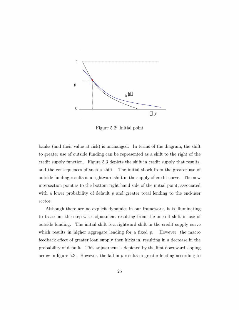
illustration, suppose there is a mapping g which maps aggregate lendingP
i �yi to
the probability of default p. To be consistent with the interpretation of higher
credit supply leading to more buoyant conditions, the function g (:) is should
be decreasing. Figure 5.2 superimposes the function g (:) on �gure 5.1. Now
consider the scenario where the advent of securitisation shifts the mix between
internal and external funding that banks use toward greater use of funding from
outside creditors. We may interpret this scenario as a decline in the entries of the
interbank matrix � such that the proportion of funding raised from outside cred-
itors increases. As argued in the previous section, such a development increases
the aggregate lending to the end-user borrowers even if the leverage of individual
9Adrian and Shin (2008c) exhibit evidence that expansions of intermediary balance sheetshelp explain future growth of GDP components such as housing investment and durable goodconsumption.
24
p
1
0∑i iy
()⋅g
Figure 5.2: Initial point
banks (and their value at risk) is unchanged. In terms of the diagram, the shift
to greater use of outside funding can be represented as a shift to the right of the
credit supply function. Figure 5.3 depicts the shift in credit supply that results,
and the consequences of such a shift. The initial shock from the greater use of
outside funding results in a rightward shift in the supply of credit curve. The new
intersection point is to the bottom right hand side of the initial point, associated
with a lower probability of default p and greater total lending to the end-user
sector.
Although there are no explicit dynamics in our framework, it is illuminating
to trace out the step-wise adjustment resulting from the one-o� shift in use of
outside funding. The initial shift is a rightward shift in the credit supply curve
which results in higher aggregate lending for a �xed p. However, the macro
feedback e�ect of greater loan supply then kicks in, resulting in a decrease in the
probability of default. This adjustment is depicted by the �rst downward sloping
arrow in �gure 5.3. However, the fall in p results in greater lending according to
25

p
1
0∑i iy
Figure 5.3: Lending boom
the argument for Proposition 1. Greater lending then feeds to lower p, and so
on. The new settling point given in �gure 5.3 is associated with a substantially
lower probability of default as well as a large stock of lending.
5.1. Subprime Lending
At the cost of some additional complexity, it would be possible to incorporate
subprime lending into the story. Suppose that the population of prime borrowers
is small relative to the expansion of total lending as implied by the new crossing
point between the credit supply curve and the macro feedback function g (:) in
�gure 5.3. Then, once all the prime borrowers have been granted a mortgage, the
banking system has to �nd additional means of creating assets. One way would be
for the banks to lend to each other. However, as discussed earlier, the aggregate
lending of the banking system to mortgage borrowers must equal the sum of the
equity and the borrowing from outside creditors. Since it is the borrowing from
the outside creditors which is increasing, the funding must ultimately �nd its way
26

to an end-user borrower.
Once all the prime borrowers in the population have a mortgage, the banks
must �nd new borrowers in order to expand their balance sheets. The only way
they can do this is to lower their lending standards. Subprime borrowers will then
start to receive funding. The mechanical nature of our framework in which banks
simply choose their balance sheet size masks important questions concerning the
short-termist nature of such lending to subprime borrowers. The answer as to why
banks would lower their lending standards in order to lend to subprime borrowers
must appeal to other frictions within the banking institutions that allows such
short-termism. Distorted incentives and shortened decisions horizons induced by
agency problems within the bank would be part of the overall story. See Rajan
(2005) and Kashyap, Rajan and Stein (2008) for discussion of such incentives.
6. Empirical Evidence
Aggregate lending to end-user borrowers by the banking system must be �nanced
either by the equity in the banking system or by borrowing from creditors outside
the banking system. The empirical counterpart to the sector described as the
\banking system" is the whole of the leveraged �nancial sector, which includes the
traditional commercial banking system, but also encompasses the market-based
�nancial system that plays a role in extending credit to banks and non-banks by
borrowing from outside creditors. In this sense, the leveraged �nancial sector
should be conceived broadly to include all leveraged institutions, such as invest-
ment banks, hedge funds and (in the US especially) the government sponsored
enterprises (GSEs) such as Fannie Mae and Freddie Mac.
27

0.0
1.0
2.0
3.0
4.0
5.0
6.0
7.0
8.0
2001 2002 2003 2004 2005 2006 2007
Trill
ion
Dol
lars
Rest of the world
Nonfinancialsectors
Nonleveragedfinancial institutions
Leveraged financialinstitutions
Figure 6.1: Holding of GSE-backed securities (source: US Flow of Funds)
6.1. Evidence from US GSE mortgage-backed securities
A complete disaggregation of the funding source for the leveraged �nancial sector
is not possible due to the lack of detailed breakdowns in the data between funding
from leveraged and unleveraged creditors. A partial picture can be obtained, how-
ever, by examining the holding of US agency and GSE-backed securities. Figure
6.1 plots the total holding of US agency and GSE-backed securities broken down
into the identity of the creditor at the end of each year from 2001 to 2007. The
data are from the US Flow of Funds accounts compiled by the Federal Reserve
(table L.210). Leveraged �nancial institutions include commercial banks, broker
dealers and other securitisation vehicles. The non-leveraged �nancial institutions
include mutual funds, insurance companies and pension funds. The \non-�nancial
sector" includes household, corporate and government sectors. Finally, the \rest
of the world" category indicates foreign creditors, especially foreign central banks
or other o�cial sector holders. Figure 6.2 charts the holders by percentage hold-
ings.
28

0%
10%
20%
30%
40%
50%
60%
70%
80%
90%
100%
2001 2002 2003 2004 2005 2006 2007
Rest of the world
Nonfinancialsectors
Nonleveragedfinancial institutions
Leveraged financialinstitutions
Figure 6.2: Holding of GSE-backed securities (percentages)
The key series for our purposes is the proportion held by other leveraged
�nancial institutions. We see that US leveraged institutions have been holding
a declining proportion of the total. At the end of 2002, leveraged �nancial
institutions held 48.4% of the total, but by the end of 2007, that percentage had
dropped to 36.7%. There has been a consequent increase in the funding provided
by the non-leveraged sector. In terms of the model, this translates to a increase in
the z vector of proportions raised from outside the \banking sector" of the model.
Notably, the holdings of the \rest of the world" category (which itself is mostly
accounted for by foreign central banks) has more than tripled from $504 billion
at the end of 2001 to $1,540 billion at the end of 2007. Recall that the increased
proportion of the funding coming from outside the banking system plays a key
role in the development of the lending boom scenario of the previous section. We
see that the assumption has some empirical support.
29

Composition of Northern Rock's Liabilities(June 1998 June 2007)
0
20
40
60
80
100
120
Jun98
Dec98
Jun99
Dec99
Jun00
Dec00
Jun01
Dec01
Jun02
Dec02
Jun03
Dec03
Jun04
Dec04
Jun05
Dec05
Jun06
Dec06
Jun07B
illio
n po
unds
Equity
Other Liabilities
Securitized notes
Retail Deposits
Figure 6.3: Source. Northern Rock annual and interim reports
6.2. Evidence from the UK
The increased importance of securitisation can be found also in the UK, from
the balance sheet series of Northern Rock, the UK bank that failed in 2007.
Northern Rock was a building society (i.e. a mutually owned savings and mortgage
bank) until its decision to go public and oat its shares on the stock market in
1997. In the nine years from June 1998 (the �rst year after demutualisation) to
June 2007 (on the eve of its crisis), Northern Rock's total assets grew from 17.4
billion pounds to 113.5 billion pounds (a constant equivalent annual growth rate
of 23.2%). By the eve of its crisis, Northern Rock was the �fth largest bank in
the UK by mortgage assets. Northern Rock's liabilities re ect both the funding
constraints it faced, as well as the way it overcame those constraints. Figure 6.3
charts the composition of Northern Rock's liabilities from June 1998 to June 2007.
Traditional deposit funding did not keep pace with total assets, and the gap was
30
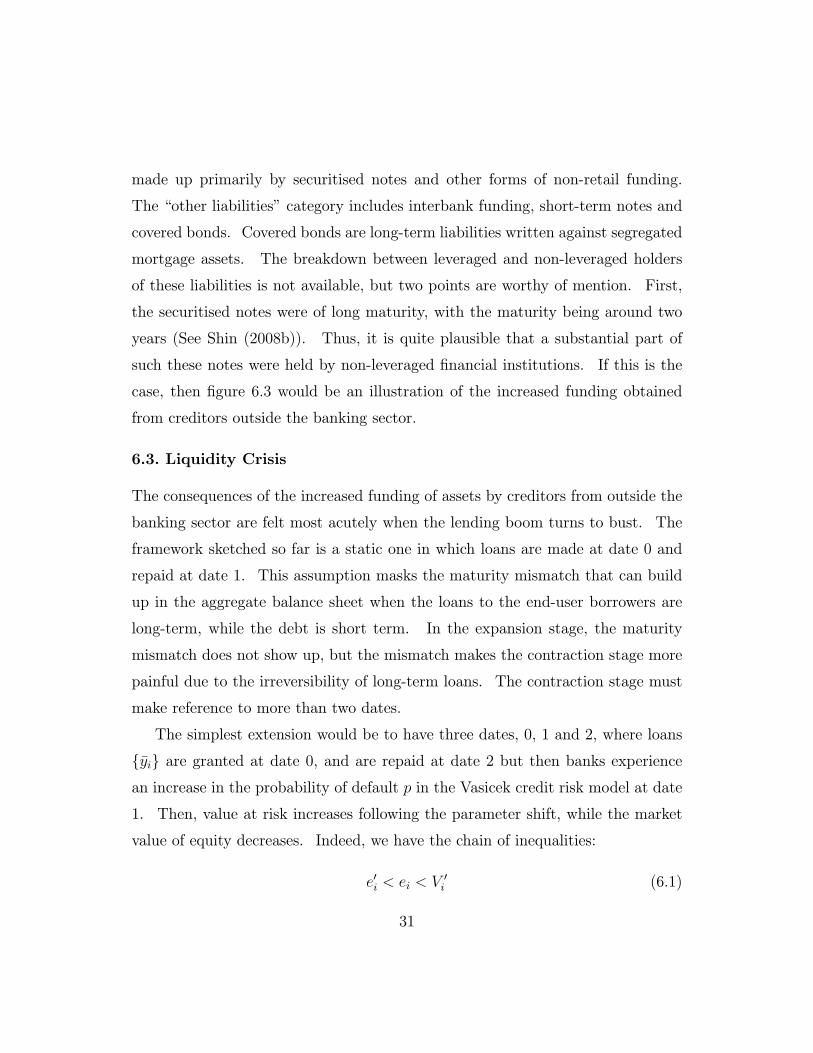
made up primarily by securitised notes and other forms of non-retail funding.
The \other liabilities" category includes interbank funding, short-term notes and
covered bonds. Covered bonds are long-term liabilities written against segregated
mortgage assets. The breakdown between leveraged and non-leveraged holders
of these liabilities is not available, but two points are worthy of mention. First,
the securitised notes were of long maturity, with the maturity being around two
years (See Shin (2008b)). Thus, it is quite plausible that a substantial part of
such these notes were held by non-leveraged �nancial institutions. If this is the
case, then �gure 6.3 would be an illustration of the increased funding obtained
from creditors outside the banking sector.
6.3. Liquidity Crisis
The consequences of the increased funding of assets by creditors from outside the
banking sector are felt most acutely when the lending boom turns to bust. The
framework sketched so far is a static one in which loans are made at date 0 and
repaid at date 1. This assumption masks the maturity mismatch that can build
up in the aggregate balance sheet when the loans to the end-user borrowers are
long-term, while the debt is short term. In the expansion stage, the maturity
mismatch does not show up, but the mismatch makes the contraction stage more
painful due to the irreversibility of long-term loans. The contraction stage must
make reference to more than two dates.
The simplest extension would be to have three dates, 0, 1 and 2, where loans
f�yig are granted at date 0, and are repaid at date 2 but then banks experiencean increase in the probability of default p in the Vasicek credit risk model at date
1. Then, value at risk increases following the parameter shift, while the market
value of equity decreases. Indeed, we have the chain of inequalities:
e0i < ei < V0i (6.1)
31

which is the mirror image of the inequalities (4.4) that hold during the boom.
The counterpart to Assumption 1 would be that the banks attempt to reduce
their total balance sheet size by reducing the size of their notional debt level �xi.
However, if the loans to end-users �yi are long-term, then banks are not free to
reduce the size of their balance sheets exibly. The constraint on the exibility
will bind harder if the proportion of assets of this type constitute a large fraction
of total assets.
In aggregate, the total long-term lending to end-users is mirrored by the size
of the funding obtained from lenders from outside the banking sector. Thus, at
an aggregate level, the increased use of securitisation is associated with a tighter
constraint against rapid reductions in balance sheet size. When value at risk
increases, banks must cut back the size of their balance sheets. Some banks will
be able to reduce their balance sheets exibly by not rolling over short-term assets
and short-term liabilities. But not every bank can do this, since the �nancial
system as a whole holds long-term illiquid assets �nanced by short-term liquid
liabilities. There will be \pinch points" that are thus exposed when value at risk
increases. These pinch point banks will su�er a liquidity crisis.
Northern Rock is a good example of such a pinch point. Its assets were almost
all long-term residential mortgages. Thus, it had very little scope to reduce its
balance sheet in a exible way once the crisis struck. Crucially, Northern Rock
was vulnerable to the tick-up in value at risk due to its high leverage. Figure
6.4 plots the leverage series from June 1998 to December 2007 according to three
di�erent measures of equity. In the early years, there was no distinction between
total equity, shareholder equity and common equity. All equity was common
equity. However, in 2005, the total equity series included for the �rst time 736.5
million pounds worth of subordinated debt, as well as 299.3 million pounds worth
of reserve notes. Both of these items had been issued much earlier (in 2001), but
32

Northern Rock's LeverageJune 1998 December 2007
10
20
30
40
50
60
70
80
90
Jun98
Dec98
Jun99
Dec99
Jun00
Dec00
Jun01
Dec01
Jun02
Dec02
Jun03
Dec03
Jun04
Dec04
Jun05
Dec05
Jun06
Dec06
Jun07
Dec07
Leverage on total equity
Leverage on shareholder equity
Leverage on common equity
Figure 6.4: Source. Northern Rock annual and interim reports
they were included in the equity series in the annual report for the �rst time in
2005.10 The inclusion of these subordinated debt items introduced a jump up in
the equity series for Northern Rock, and accounts for the sharp jump down in the
leverage series in June 2005 in �gure 6.4. However, as we can see also from �gure
6.4, when the subordinated debt items are excluded, and equity is construed just
as shareholder equity, the leverage series continues to move up in 2005. On the
eve of its crisis in 2007, the leverage ratio on common equity stood at almost 60.
This made Northern Rock particularly vulnerable among UK banks to the credit
crisis that erupted in August 2007.11
Although the coventional notion of equity in bank regulation is as a bu�er
against losses to depositors, the relevant equity measure for funding constraints is
10See Shin (2008b).11See Yorulmazer (2008) for an empirical analysis of UK banks at the time of the Northern
Rock crisis.
33

the stake of held by those who control the assets - i.e. the common equity holders.
The distinction is seen most clearly for repurchase agreements (repos), where the
haircuts applied by creditors determine the permitted leverage (see Adrian and
Shin (2008b)). Thus, even though the Basel-style leverage ratios were kept low by
issuing subordinated debt and preferred equity, the e�ective leverage for funding
purposes was climbing very rapidly in the case of Northern Rock. Its run in the
summer of 2007 should be seen in this context.
7. Related Literature and Conclusions
The importance of securitisation for �nancial stability lies in the impact of the
shadow banking system to a�ect the total supply of credit to end-users. When
there is a decline in the riskiness of fundamental assets (in our case, through a
fall in the parameter p), the risk-taking capacity of the shadow banking system
increases.
The idea that the changes in the lender's balance sheet is important in de-
termining the supply of credit has also �gured in an earlier literature that has
emphasized the liquidity structure of the banks' balance sheets (Bernanke and
Blinder (1988), Kashyap and Stein (2000)), or the cushioning e�ect of the banks'
regulatory capital (Van den Heuvel (2002)).
The supply-side mechanism for the growth of credit should be distinguished
from the larger literature on the uctuations in credit due to the shifts in the
demand for credit, as emphasized for instance by Bernanke and Gertler (1989)
and Kiyotaki and Moore (1998, 2001). The key to the demand-side explanations
of the uctuation of credit is the changing strength of the borrower's balance sheet
and the resulting change in the creditworthiness of the borrower.
The mechanism proposed here is in line with the supply side explanation for
the subprime crisis. The greater risk-taking capacity of the shadow banking
34

system leads to an increased demand for new assets to �ll the expanding balance
sheets, and an increase in leverage. The picture is of an in ating balloon which
�lls up with new assets. As the balloon expands, the banks search for new assets
to �ll the balloon. They look for borrowers that they can lend to. However,
once they have exhausted all the good borrowers, they need to scour for other
borrowers - even subprime ones. The seeds of the subsequent downturn in the
credit cycle are thus sown.
According to the picture painted here, the subprime crisis has its origin in
the increased supply of loans - or equivalently, in the increased appetite for new
assets to �ll up the expanding balance sheets. In this way, it is possible to explain
two features of the subprime crisis - �rst, why apparently sophisticated �nancial
intermediaries continued to lend to borrowers of dubious creditworthiness, and
second, why such sophisticated �nancial intermediaries held the bad loans on their
own balance sheets, rather than passing them on to other unsuspecting investors.
Both facts are explained by the imperative to expand balance sheets during an
upturn in the credit cycle.
35

References
Adrian, T. and H. S. Shin (2007) \Liquidity and Leverage" working paper, Federal
Reserve Bank of New York and Princeton Universityhttp://www.princeton.edu/~hsshin/working.htm
Adrian, T. and H. S. Shin (2008a) \Liquidity and Financial Contagion" Banque
de France Financial Stability Review, 11, 1 - 8.
Adrian, T. and H. S. Shin (2008b) \Financial Intermediary Leverage and Value at
Risk" working paper, Federal Reserve Bank of New York and Princeton Universityhttp://www.princeton.edu/~hsshin/working.htm
Adrian, T. and H. S. Shin (2008c) \Financial Intermediaries, Financial Stabilityand Monetary Policy" paper for the Federal Reserve Bank of Kansas City Sym-posium at Jackson Hole, 2008http://www.princeton.edu/~hsshin/working.htm
Alizalde, A. and R. Repullo (2006) \Economic and Regulatory Capital in Banking:What is the Di�erence?" working paper, CEMFI.
Ashcraft, A. and T. Schuermann (2008) \Understanding the Securitization ofSubprime Mortgage Credit" Sta� Report 318, Federal Reserve Bank of New Yorkhttp://www.newyorkfed.org/research/sta� reports/sr318.pdf
Bank for International Settlements (2008) 78th Annual Report, Basel, Switzerland.
Bernanke, B. and A. Blinder (1988) \Credit, Money and Aggregate Demand"
American Economic Review, 78, 435-39.
Bernanke, B. and M. Gertler (1989) \Agency Costs, Net Worth, and Business
Fluctuations" American Economic Review, 79, 14 - 31.
Brunnermeier, Markus (2008) \De-Ciphering the Credit Crisis of 2007," forth-
coming, Journal of Economic Perspectives.
Demyanyk, Y. and O. van Hemert (2007) \Understanding the Subprime MortgageCrisis" working paper, New York University, Stern School of Business.
36

Eisenberg, L. and T. H. Noe (2001) \Systemic Risk in Financial Systems" Man-agement Science, 47, 236-249.
Gieve, J. (2008) \The Return of the Credit Cycle: Old Lessons in New Markets"
speech at the Euromoney bond investors congress, February 27, 2008http://www.bankofengland.co.uk/publications/speeches/2008/speech338.pdf
Gorton, G (2008) \The Panic of 2007" paper for the Federal Reserve Bank of
Kansas City Symposium at Jackson Hole, 2008
Gorton, G. and N. Souleles (2006) \Special Purpose Vehicles and Securitization"in R. Stulz and M. Carey (eds) The Risks of Financial Institutions University ofChicago Press, Chicago.
Greenlaw, D., J. Hatzius, A. Kashyap and H. S. Shin (2008) \Leveraged Losses:Lessons from the Mortgage Market Meltdown" Report of the US Monetary Mon-etary Form, number 2.http://www.chicagogsb.edu/usmpf/docs/usmpf2008confdraft.pdf
International Monetary Fund (2008) Global Financial Stability Report, April,Washington DC
Kashyap, A., R. Rajan and J. Stein (2008) \Rethinking Capital Regulation" paperfor the Federal Reserve Bank of Kansas City Symposium at Jackson Hole, 2008
Kashyap, A. and J. Stein (2000) \What Do a Million Observations on Banks Sayabout the Transmission of Monetary Policy?" American Economic Review, 90,
407-428.
Keys, Benjamin, Tanmoy Mukherjee, Amit Seru and Vikrant Vig (2007) \DidSecuritization Lead to Lax Screening? Evidence From Subprime Loans" working
paper, University of Chicago GSB.
Kiyotaki, N. and J. Moore (1998) \Credit Chains" LSE working paper,
http://econ.lse.ac.uk/sta�/kiyotaki/creditchains.pdf.
Kiyotaki, N. and J. Moore (2001) \Liquidity and Asset Prices" LSE workingpaper, http://econ.lse.ac.uk/sta�/kiyotaki/ liquidityandassetprices.pdf.
37

Mian, Atif and Amir Su� (2007) \The Consequences of Mortgage Credit Expan-sion: Evidence from the 2007 Mortgage Default Crisis" working paper, Universityof Chicago GSB
Milgrom, P. and J. Roberts (1994) \Comparing Equilibria" American Economic
Review, 84, 441-459.
Mishkin, F. (2008) \On `Leveraged Losses: Lessons from the Mortgage Market
Meltdown"' discussion at 2nd US Monetary Policy Forum, New York, February27th 2008http://www.federalreserve.gov/newsevents/speech/mishkin20080229a.htm
Rajan, R. (2005) \Has Financial Development Made the World Riskier?" Pro-ceedings of the Federal Reserve Bank of Kansas City Symposium at Jackson Hole,2005.http://www.kc.frb.org/publicat/sympos/2005/sym05prg.htm
Shin, H. S. (2008a) \Risk and Liquidity in a System Context" Journal of FinancialIntermediation, 17, 315 - 329.
Shin, H. S. (2008b) \Re ections on Modern Bank Runs: A Case Study of North-ern Rock" working paper, Princeton University
Van den Heuvel, S. (2002) \The Bank Capital Channel of Monetary Policy",working paper, Wharton School, University of Pennsylvania,http://�nance.wharton.upenn.edu/~vdheuvel/BCC.pdf
Vasicek, O. (2002) \The Distribution of Loan Portfolio Value"
http://www.moodyskmv.com/conf04/pdf/papers/dist loan port val.pdf
Yorulmazer, T. (2008) \Liquidity, Bank Runs and Bailouts: Spillover E�ects Dur-
ing the Northern Rock Episode" working paper, Federal Reserve Bank of New
York.
38