sectorial holdings and stock 2021 prices: the …
TRANSCRIPT

SECTORIAL HOLDINGS AND STOCK
PRICES: THE HOUSEHOLD-BANK NEXUS2021
Matías Lamas and David Martínez-Miera
Documentos de Trabajo
N.º 2130

SECTORIAL HOLDINGS AND STOCK PRICES:
THE HOUSEHOLD-BANK NEXUS

Documentos de Trabajo. N.º 2130
September 2021
(*) We thank Andrés Almazán, Carmen Broto, Ángel Estrada, Javier Mencía, Carlos Pérez, Rafael Repullo, Sheridan Titman, and seminar audiences at the Banco de España for their comments and suggestions, all errors are our own. We are also grateful to the Statistics Department of the Banco de España for their help and support regarding the Securities Holdings Statistics by Sector. We acknowledge financial support from the Spanish Ministry of Economics and Competitiveness, Grants No. ECO2015-68136-P (Martínez-Miera). This paper reflects our views and not necessarily the views of Banco de España or the Eurosystem. Matías Lamas e-mail: [email protected]. David Martínez-Miera, e-mail: [email protected].
Matías Lamas
BANCO DE ESPAÑA
David Martínez-Miera
UC3M AND CEPR
SECTORIAL HOLDINGS AND STOCK PRICES:
THE HOUSEHOLD-BANK NEXUS (*)

The Working Paper Series seeks to disseminate original research in economics and fi nance. All papers have been anonymously refereed. By publishing these papers, the Banco de España aims to contribute to economic analysis and, in particular, to knowledge of the Spanish economy and its international environment.
The opinions and analyses in the Working Paper Series are the responsibility of the authors and, therefore, do not necessarily coincide with those of the Banco de España or the Eurosystem.
The Banco de España disseminates its main reports and most of its publications via the Internet at the following website: http://www.bde.es.
Reproduction for educational and non-commercial purposes is permitted provided that the source is acknowledged.
© BANCO DE ESPAÑA, Madrid, 2021
ISSN: 1579-8666 (on line)

Abstract
We analyze the evolution and price implications of aggregate sectorial holdings of stocks,
using detailed information on the universe of publicly traded stocks in the euro area. We
document that: i) households’ (HH) direct holdings represent a higher fraction of total
ownership in domestic bank stocks than in non-fi nancial corporation (NFC) stocks; ii)
HH holdings of stocks increase (decrease) following a decline (increase) in the stock
price, especially for domestic bank stocks; and iii) an increase in domestic HH holdings
is followed by future (persistent) increases in the price of NFC stocks, but not for bank
stocks. Moreover, during equity issuances, an increase in the share of domestic HH
holdings is followed by a future (persistent) decrease in the stock price of bank stocks,
but not for NFC stocks. Our results are consistent with HH being liquidity providers in
the stock market, and at the same time subject to negative information asymmetries. We
argue that this latter effect is more prevalent in domestic bank stocks than in NFC given
the close relationships between HH and banks.
Keywords: household ownership, stock prices, equity issuance, banks, non-fi nancial
corporations, liquidity provision, informational asymmetries.
JEL classifi cation: G11, G14, G21, G50.

Resumen
Este trabajo analiza la evolución y las implicaciones en el precio de las acciones de las
tenencias de acciones por parte de distintos sectores. Para ello se utiliza información
detallada sobre el universo de acciones cotizadas de la zona del euro. Se encuentra lo
siguiente: i) los hogares cuentan con un mayor peso en el accionariado de los bancos
que en el de las empresas no fi nancieras; ii) las tenencias de acciones de los hogares
aumentan (disminuyen) cuando cae (sube) el precio de las acciones, especialmente
cuando se trata de las acciones de bancos nacionales, y iii) un aumento de las tenencias
de acciones de los hogares domésticos es seguido por incrementos persistentes del
precio de las acciones de las empresas, mientras que esto no ocurre para los bancos.
Además, tras una emisión de acciones, un aumento de la participación de los hogares
en el accionariado de los bancos es seguido por una caída del precio de estas acciones,
mientras que esto no ocurre en las empresas. Nuestros resultados sugieren que los
hogares actúan como proveedores de liquidez en los mercados de acciones, si bien al
mismo tiempo están sujetos a asimetrías de información. Este último mecanismo puede
ser más relevante cuando los hogares compran las acciones de los bancos, dadas las
estrechas relaciones entre las entidades y los hogares.
Palabras clave: participación de los hogares en el mercado de acciones, precio de las
acciones, emisiones de acciones, bancos, empresas no fi nancieras, provisión de liquidez,
asimetrías de información.
Códigos JEL: G11, G14, G21, G50.

BANCO DE ESPAÑA 7 DOCUMENTO DE TRABAJO N.º 2130
1. Introduction
What are the roles of different sectors when investing in the stock market? Do
households play a different role in bank than in non-financial corporation stocks?
Households’ direct holdings of stocks represent a sizeable part of the stock market.
According to the Securities Holdings Statistics by Sector (SHSS), euro area households’
(HH) direct holdings of stocks accounted for 10% of total stock market capitalization of
euro area firms as of the end of 2017.1 In order to understand the role of HH direct
investment in the stock market, we analyze (aggregate) trading behavior of HH, and that
of other sectors, and its implications for future price developments. In doing so we
highlight the different patterns present in bank stocks with respect to non-financial
corporations (NFC), as well as between domestic and foreign investors.
We document that in our sample: (i) bank stocks represent a larger fraction of direct
holdings for HH than for other market participants, especially for bank stocks with which
the HH shares residence (domestic); (ii) HH increase their direct holdings after price
declines in a given stock, especially for domestic bank stocks; (iii) after an increase in
(domestic) HH direct ownership in a given NFC stock the stock price increases, but bank
stock prices do not; (iv) in equity issuances, an increase in (domestic) HH direct
ownership is followed by future price declines in bank stocks, but not in NFC stocks.
Our interest in HH direct investment is based on two facts. First, HH direct holdings
are large and, as suggested by recent events (such as the “GameStop short squeeze”, IMF
(2021)), can have implications in the stock market if the market is not fully efficient.
Second, HH are a special type of investor when compared to other participants in the
stock market (institutional investors). HH have different liquidity needs than other
participants –liquidity channel-, but also have lower financial sophistication -information
channel–. Given the close relationships that HH have with banks with respect to financial
investment decisions (as banks have close ties with their clients), we focus on
documenting the existing differences between HH and other sectors’ trading patterns
when trading bank versus NFC stocks. These differences allow us to highlight the
potential frictions that HH face in the stock market, and their aggregate price implications.
1 HH holdings refer to the market value of listed, ordinary stocks of the euro area in HH portfolios.
To perform our analysis, we use data from the SHSS. This dataset identifies
aggregate sectorial holdings for each publicly traded security in the euro area on a

BANCO DE ESPAÑA 8 DOCUMENTO DE TRABAJO N.º 2130
quarterly basis. One of the advantages is that it identifies aggregate HH direct holdings,
as well as those of other sectors such as mutual funds (MF), insurance and pension funds
(IPF), banks or NFC. In doing so it identifies the residence of the holder, allowing us to
differentiate between domestic and foreign investors for each investor type. To the best
of our knowledge, this is the first study that, using the universe of holdings of publicly
traded stocks in Europe for the period 2009-2017, explores the dynamic relationships
between price developments and aggregate stock holdings of HH and other sectors, and
documents stark differences between domestic and foreign HH (as well as other sectors)
when trading bank or NFC stocks.
Analyzing HH direct holdings and comparing them to other sectors is relevant as
HH can have a different role than other market participants in the stock market. Previous
research has shown that HH can play the role of liquidity providers in the stock market
and invest when prices are low due to liquidity tensions (e.g. Kaniel et al. 2008) –liquidity
channel-.2 However, HH have also been shown to be less sophisticated and less informed
than other participants in the stock market (Barber and Odean, 2000 and Barber et al.
2009) and, hence, can be slower and less efficient in incorporating new information about
stock fundamentals –information channel-. This latter effect can be more relevant for
domestic investors, as less sophisticated investors have been shown to have a higher home
bias (Karlson and Norden 2007). Hence, the information channel can make (domestic)
HH more prone to buy stocks that, due to a negative information shock which HH do not
fully incorporate, have a decline in their future price. If such information is not
instantaneously absorbed in the stock price, it will continue to decline in the future up to
the moment in which the information is completely incorporated.
If HH are subject to a (negative) information channel, HH can act not only as
liquidity providers, buying when the price goes down because of liquidity tensions and
obtaining positive profits when such tensions cease to exist, but can also be subject to a
“lemons” problem, buying when the price goes down because some (better informed)
market participants are receiving negative signals about the stocks’ fundamentals and are
selling the stock. In such case HH would make a loss on such trade.
We argue that the close relationship that banks have with their clients (HH), to
which they offer advice and special conditions if they invest in their own stocks (Hoechle
2 See Timmer (2018) for evidence on how liquidity needs between institutional investors (investment funds and pension funds or insurance companies) affect buying or selling debt securities after a price decline.

BANCO DE ESPAÑA 9 DOCUMENTO DE TRABAJO N.º 2130
et al. 2018), can make the informational asymmetry higher in bank stocks than in NFC
stocks. This can be more relevant when bank and holder share nationality, i.e. domestic
banks, as it is more probable that such investors share a relationship with the bank.
This study provides evidence consistent with both a liquidity and informational
channel in HH stock investing. Our evidence suggests that informational asymmetries
can be especially relevant in the case of domestic bank stocks, which we argue can be
related to the close relationships between HH and banks in making financial decisions.
In line with the close relationship that HH and banks have, we document in Section
2 that the weight of HH direct holdings in bank stocks is higher than in NFC stocks, and
that this is especially the case when banks and HH share the same residence (domestic
banks), which we argue is a proxy of the closeness of such relationship. At the end of
2017 HH direct holdings represented 13.8% of the market capitalization of euro area bank
stocks, versus 9.6% in the case of NFC stocks. This “bias” towards bank stocks is more
prominent when we split holdings of the HH sector on the basis of its residence. Direct
holdings of HH that share residence with the headquarter of banks (exposures of domestic
HH to domestic banks) represented 13.0% of the market capitalization of the euro banking
sector as of the end of 2017 (8.7% in the case of NFCs). This percentage falls significantly
to 0.8% for foreign HH (HH that do not share residence with the bank) and, importantly,
is similar to holdings of NFC stocks by foreign HH, which is 0.9%.
After documenting the differences in aggregate stock holdings of different
(domestic and foreign) sectors, in Section 4 we analyze the aggregate trading patterns of
HH (and other sectors) following a decline (increase) in stock prices, and their differences
in bank versus NFC stocks. We also analyze if domestic investors in each given sector
buy more (or less) stocks after a price decrease than foreign investors in such sector. We
then analyze in Section 5 if changes in (domestic) HH holdings (or those of any other
sector) are related to future price changes, studying if there are differences in this
relationship in bank versus NFC stocks. We analyze both normal times and also periods
of equity issuances, as such periods are ones of high informational asymmetries between
the firm and its investors (Myers and Majluf, 1984 and Miller and Rock, 1985).
Regarding our first set of results, we document that HH, as well as NFC, increase
(reduce) their holdings in a given stock the quarter after a drop (increase) in the price of
the stock. On the other hand, institutional investors, mainly MF and banks, reduce

BANCO DE ESPAÑA 10 DOCUMENTO DE TRABAJO N.º 2130
(increase) their holdings the quarter after a drop (increase) in the stock price. We find that
this pattern of HH direct investment is more relevant in bank stocks than in NFC stocks
and that such pattern is driven by domestic HH and not by foreign HH. In particular, a
decline of one standard deviation in NFC prices (-15%) leads to a modest increase of
domestic HH holdings of 0.5%. The change in holdings is five times greater for the same
shock in bank stock prices. Similarly, we also document the existence of a differential
behavior of domestic vs foreign NFC holders in the case of bank stocks. Finally, we show
how the reaction to price decreases by domestic HH and NFC in bank stocks is four times
larger than to price increases. This is not the case for other sectors such as IPF, MF or
banks. This result highlights that during periods of negative bank shocks (which translate
into stock prices declines) there is an increase in the holdings of domestic HH and NFC
(and not of banks, IPF or MF).
Concerning our second set of results, we find that an increase in the share of
domestic HH holdings predicts future permanent increases in NFC stock prices. This
result is in line with the liquidity provision mechanism present in Kaniel et al. (2008)
among others. The argument is as follows: HH act as liquidity providers in moments of
price pressure that drive the stock price down and buy the stock at a depressed price. Once
the price pressure lifts HH benefit from the reversal of such stock price to its original
fundamental price. Interestingly, we find that this is not the case in bank stocks, as we
document that an increase in the share of domestic HH holdings does not predict future
increases in bank stock prices. This latter result suggests a potential negative information
channel that domestic HH can be subject to when buying (bank) stocks – information
channel-. Consistently with domestic HH having a closer link with banks than foreign
HH, we find that an increase in the share of foreign HH holdings predicts an increase, and
not a decline, in bank stock prices in the future.
Finally, in order to further analyze the relevance of the potential negative
informational asymmetries that HH can be subject to when trading stocks, we study equity
issuances. We do so as equity issuances are situations in which the asymmetries of
information between investors and the firm managers can heighten. Our last set of results
documents that when during an equity issuance of bank stocks the share of domestic HH
holdings increase, this is followed by future persistent price declines in the following
quarters. In particular, for follow-on (seasoned) issuances of bank stocks an increase in
HH holdings of one standard deviation leads to a decline in the price per share of 15%

BANCO DE ESPAÑA 11 DOCUMENTO DE TRABAJO N.º 2130
(on average) four quarters after the issuance, and this effect is persistent.3 This finding is
consistent with HH being less informed than other investors about the underlying reason
of the equity issuance and, therefore, the underlying quality of the stock -information
channel-. In this respect, we document that these aforementioned results are only present
in equity issuances of bank stocks and not in equity issuances of NFC, and only present
when the increase is in domestic (and not foreign) HH share.
We end our analysis by performing, in Section 6, several tests that ensure the
robustness of our results. We first perform our analysis undergoing a seemingly unrelated
regression, instead of an OLS, procedure. We then restrict our sample to focus only on (i)
bank and NFC stocks that are of similar (large) market value and (ii) periods in which the
aggregate price trends of both bank and NFC stocks are also similar. We find that our
results hold in all these robustness checks.
Our novel findings highlight the aggregate implications of underlying frictions in the
stock market. Our study suggests that the HH sector plays a liquidity role in the stock
market, and at the same time is subject to informational asymmetries, which are larger in
the case of domestic bank stocks. We argue that this can have non-trivial effects for the
economy. By providing liquidity in the market, HH can help ameliorate negative feedback
loops in stock prices. However, this can come at a financial cost for HH if such prices do
not revert, which we find is more prevalent in bank stocks. Also the fact that domestic
HH holdings increase during distress situations (stock price declines), and that banks'
3 By focusing on price performance the quarters after the issuance takes place we avoid possible mechanical price dilution effects that occur during the quarter in which the issuance takes place.
equity issuances expose HH to informational asymmetries, can affect regulators’
incentives and decision making in relevant ways.
1.1. Related literature
This study is related to two strands of research. The first strand of literature comprises
those studies analyzing the stock trading behaviors of different agents. We contribute to
this literature by being the first ones that analyze aggregate direct HH stock holdings and
document the important differences that exist between the buying and selling patters in
bank and NFC stocks and in domestic and foreign investors of each holder-sector.
Keniel et al (2008) provides evidence on how individual investors buy stocks
following price declines in the previous month and how, in doing so, they obtain abnormal

BANCO DE ESPAÑA 12 DOCUMENTO DE TRABAJO N.º 2130
returns. They argue that this evidence is consistent with individual investors being risk
averse and playing a liquidity role in the stock market. Timmer (2018) provides evidence
on how institutional investors subject to liquidity pressures are more prone to sell bonds
which are bought by institutions with lower liquidity pressures obtaining a profit in doing
so. Our results complement the ample literature on trading behaviour of different types
of investors, by providing evidence on the relevance of HH direct holdings and showing
the different patterns that occur in bank stocks and NFC stocks as well as between foreign
and domestic investors. We argue that our novel findings are also in line with the presence
of asymmetries of information, and not only liquidity provision, being especially relevant
for HH trading in bank stocks.
Evidence in Gibson et al. (2004) and Chemmanur et al (2009) highlights that
institutional investors trading during an equity issuance is a predictor of future stock
performance. Such studies conclude that institutional investors, by being more informed
than other investors, are able to obtain positive returns during equity issuances. We add
to this previous results by providing relevant information on other important agents in the
stock market, HH, and showing that increases in domestic HH ownership patters are
predictors of future negative stock performance for banks but not for NFC following an
equity issuance.
The second strand of literature related to our study is the one analyzing the
important role that banks have in household financial decisions. We complement this
literature by providing evidence of the aggregate effect of such relations. We show that
HH show different trading patterns when trading bank stocks than NFC stocks and that
this is especially true when they share residence with the bank. Hoechle et al. (2018)
shows evidence consistent with bank financial advisors favoring the interest of the bank
when advising clients, and these advices resulting in worse results for the client. Golez
and Marin (2015) find similar incentives problems related to trading decisions of bank
affiliated-funds. We show evidence consistent with these incentive problems having a
(negative) impact for domestic HH trading behaviour in bank stocks.
The remainder of the paper is structured as follows. Section 2 presents the data
sources used for our analysis as well as descriptive statistics of our variables of interest.
Section 3 details our estimation methodology. Section 4 presents the results of our
estimations related to the evolution of sectorial holdings following a price change and
Section 5 presents the results regarding the evolution of stock prices after changes in

BANCO DE ESPAÑA 13 DOCUMENTO DE TRABAJO N.º 2130
sectorial holdings. Section 6 performs different robustness checks that show how our
main results are robust to different empirical specifications and sample selections and
finally section 7 presents our concluding remarks.
2. Data
This section provides in section 2.1 a description of the data sources used in our
analysis, and in section 2.2 descriptive statistics of the variables used in our study
differentiating between bank stocks and NFC stocks.
2.1. Data sources
Our dataset is constructed using the SHSS, a large repository of holdings of
securities collected by the Eurosystem. The SHSS covers, on a quarterly basis, aggregate
holdings of securities of institutional (e.g. mutual funds, insurance companies, pension
funds) and retail sectors (mainly, HH and NFC) based in euro area countries and in the
rest of the world, albeit with limitations for this latter case. Holdings are directly reported
to the Eurosystem or collected via custodians, which ensures a comprehensive coverage,
particularly from Q4 2013 onwards.4 The main advantage of this database is that holdings
data is available on a security-by-security basis, allowing for a granular view of stocks
holdings over time. In addition, the SHSS collects some characteristics of securities, such
as their prices or market capitalization.
Our main interest is in holdings of common stocks issued by euro area
counterparties. To obtain this information, we use the equity module of the SHSS, which
includes common stocks as well as other equity instruments (e.g. preferred shares). We
focus on common stocks and match our sample with the Centralised Securities Database
(CSDB) –also run by the Eurosystem-, which contains a richer set of attributes per
security. The final sample comprises holdings per institutional sector and country of
3,889 stocks from Q1 2009 to Q4 2017, of which 3,300 are NFC stocks, 131 are bank
stocks and 458 are shares issued by non-bank financials.5 Our set of stocks comprise all
4 Before Q4 2013 there are some gaps in holdings data in certain countries. When not reliable, we have dropped these holdings from our dataset. Holdings coverage is almost complete after that date. For instance, Fache and Rodríguez (2018) show that in Q4 2015 the coverage of SHSS holdings reached nearly 93% of that recorded in the euro area accounts. It is important to note that such study refers to holdings of equity and debt instruments, while we focus on euro area common stocks. 5 When compared to the Securities issues statistics (SEC) of the European Central Bank, our sample covers on average 93% of the total market capitalization of listed shares in the euro area.

BANCO DE ESPAÑA 14 DOCUMENTO DE TRABAJO N.º 2130
when new shares are issued. For this subset of periods, we differentiate follow-on
(seasoned) issuances from other issuances (e.g. scrip dividends) by merging our data with
that of the Deal Screener of Refinitiv.
listed shares, including delisted stocks provided that they were active at some point during
the sample period. Finally, for each common stock the CSDB allows to identify periods
6 In this quarter, we cover 95.1% of the market capitalization of all euro area common stocks, according to ECB´s SEC statistics. Holdings coverage, or the ratio of holdings to market capitalization, is 87.8% for financials (95.6% in the case of banks stocks), and 90.7% for NFC stocks. 7 When calculating aggregate holdings of euro area HH, we consider French non-profit institutions serving households (NPISH) within the French HH sector as we cannot separate HH holdings from NPISH holdings in this country. 8 Holdings of the RoW are subject to the so-called custodian bias as the client of the non-euro area custodian that reports holdings may be another custodian, with clients in the euro area. 9 Given the incomplete disclosure of RoW our rows in Panel B do not add up to 100%.
2.2. Holdings data
2.2.1. Holdings at a glance
Table 1 summarizes holdings of euro area common stocks as of the end of 2017,
which is the last observation in our dataset. Holdings are broken down into issuer sectors
(rows) and holder sectors (columns). There are two main issuer categories, financials,
which includes the subsegment of banks, and NFC.6 Holders are euro area institutional
sectors and are divided into HH (individual investors), NFC, Banks, insurance and
pension funds (IPF), mutual funds (MF), and “Other”. “Other” comprises all remaining
categories (e.g. holdings of the public sector or direct investment of financial holdings,
among others).7 We also show holdings of investors based in the Rest of the World
(RoW). It is important to highlight that for this sector data is less reliable given the lower
informational requirements for non-European investors.8 The table is split into three
panels. Panel A collects the distribution of holdings in EUR bn. Panels B and C describe
the weight of holdings in total market capitalization as well as the distribution of holdings
per sector, respectively.9
Table 1 shows that HH are major holders of euro area common stocks, especially
in the case of banks. HH direct holdings accounted for EUR 753 bn in Q4 2017 (Panel
A), representing 10.0% of the total market capitalization of our set of common stocks
(Panel B). Interestingly, while HH ownership stands at 9.6% in the NFC segment, it
reaches 13.8% for banks, being this share much higher than that of NFC and other euro

BANCO DE ESPAÑA 15 DOCUMENTO DE TRABAJO N.º 2130
area institutional investors such as Banks and IPF, and comparable to that of MF.10 This
result barely changes when we consider holdings in previous quarters (see Figures 1.A to
1.C). Although not shown in the table, we note that HH ownership of banks is very
different across jurisdictions. For instance, in Spain, where banks predominantly focus
on retail activities, the share of HH in total banks´ equity more than doubles that of their
European peers (25.9%).
The preference of HH for bank stocks is further confirmed when looking at each
sector’s investment portfolio, i.e. the distribution of holdings per equity segment (Table
1 Panel C). In Q4 2017, holdings in bank stocks represented 13.4% of the portfolio of
common stocks of HH. Only the allocation of Banks holders and “Other” holders towards
these stocks is higher, which could be due to holdings of own stocks in the former case,
and the role of strategic investors and semi-public entities in the so-called “Other”
sector.11 In Table A1 in the appendix, we provide further evidence showing that this bias
towards bank stocks is fundamentally driven by domestic investors, especially HH.
Interestingly, the allocation towards banks is much higher for domestic HH than for non-
domestic HH. For domestic HH banks represent 14.0% of their direct holdings versus
7.9% for non-domestic HH (1.8 times more -Table A1 Panel C-), while for domestic HH
NFC stocks represent 75.9% of their portfolio versus 69.3% for non-domestic HH (1.1
times, -Table A1 Panel C-)
A further analysis of HH ownership reveals that HH share is not always higher in
banks than in NFC stocks. Figure 2 shows the (average) share of HH in the two types of
common stocks by quintiles of the distribution of the market capitalization of banks (as
before, data refers to the last data point –Q417-). In the first quintile, which concentrates
53% of all NFC (NFC are on average smaller than banks), HH ownership is higher in this
sector than in financial companies. As the market capitalization of companies grows, HH
ownership diminishes in the case of NFC, while in banks this trend is less clear. It is
relevant to note how in the second, fourth and fifth quintiles, the share of HH becomes
10 The share of the RoW in the market capitalization of euro area stocks stands at 37%, or 41% of total holdings in the SHSS. This is similar to the documented by Fache and Rodríguez (2015) for quoted shares (which includes common stocks and other types of shares) using this same database. Holdings data in that work refers to Q4 2013. 11 For illustrative purposes, Table A1 shows holdings information differentiating between domestic and non-domestic holders. The main messages of this section hold. In particular, the allocation of domestic HH towards bank stocks is higher than that of NFC, IPF and MF holders.

BANCO DE ESPAÑA 16 DOCUMENTO DE TRABAJO N.º 2130
more important in banks than in NFC. For illustrative purposes, a histogram depicting the
complete distribution of HH ownership in the two stock types is presented in Figure 3.12
Overall, the aggregate size of HH exposures suggests that the trading behavior of
this sector might be relevant in driving price developments in stocks. On the other hand,
the role of HH could be different in banks than in NFC given the concentration of HH
holdings in the former stocks, and the ties of retail customers with their banks.
Table 3 focuses on domestic HH (those who invest in securities of their own
country) and examine changes in ownership and future price performance. is
our results are not affected by these periods. Finally, we note that we do not know whether the RoW is a net buyer of net seller of securities as holdings data is less reliable for this sector.
12 Our main results control for stock fixed effects which ameliorate concerns regarding differences in unobservable characteristics among stocks. In order to further analyze possible comparability issues we analyze different subsets of stocks in section 6.2. 13 The institutional sectors in this study (Banks, IPF and MF) are the same as those in Timmer (2018) 14 We note that netbuy is higher than zero for all holders. This happens for different reasons. First, netbuy is positively skewed, and positive changes in holdings are, on average, slightly higher than negative changes (which increases the mean of netbuy above zero). Second, netbuy tends to be much higher than zero in periods in which the number of shares issued augments (within the same firm). Excluding these periods (14% of total observations), the mean of netbuy is closer to zero (and even negative for bank holders). In the empirical part, we have performed some exercises (available upon request) to ensure that
Table 2 and 3 summarize the main variables of interest for the empirical analysis.
Table 2 describes trading behavior variables and price changes for each holder:
netbuy and return. Netbuy is the (average) quarterly change in stock holdings, measured
as the number of shares held (expressed in logs) and calculated at the security level (we
multiply this variable by 100 for expositional purposes). Return stands for the lagged
return of the stock (its price change in the previous quarter). We focus on five holder
types, HH, NFC, Banks, IPF and MF, and two issuer or equity segments, banks and
NFC.13 Holders are shown in columns, while issuers in rows. Panel A refers to the sample
of Banks, Panel B to NFC, and Panel C to Banks and NFC.
The number of observations is larger for HH than for other holders as there are more
groups of this type of investor (more countries of residence). Except for IPF holders,
netbuy is higher in banks than in NFC issuers, i.e. holdings increase (on average) more
when investors trade bank versus NFC securities. Netbuy is also higher in HH than in
other holders. It is also relevant to note that the standard deviation of netbuy is pronounced
across firms and holders.14
2.2.2. Summary statistics

BANCO DE ESPAÑA 17 DOCUMENTO DE TRABAJO N.º 2130
the percentage change in the share of domestic HH ownership per security, being the
share the ratio between the number of shares held by domestic HH to the total number of
shares. Future price performance is the cumulative change in the log of prices at future
horizons. For instance, in the second column of this panel, reflects price
changes between quarter t+1 and t, while in the third column takes the
cumulative price change between quarter t+2 and t. , in the final column, is
the cumulative price change between quarter t+8 and t, or two years after.
The mean value of ∆dshare is slightly positive for the full sample (Panel C), being
somewhat lower for banks (Panel A) than for NFC (Panel B). With regards to future
returns, future price changes are (on average) positive in NFC but negative for banks
stocks. The underperformance of banks is expected as our sample period (2009-2017)
covers the financial and the sovereign crisis, when banks stocks were severely hit.15
Standard deviations are large, particularly for longer horizons, and similar between the
two firm types.
15 In table A10 we perform our analysis focusing only in periods in which the aggregate price trends are similar both for bank and NFC stocks. See section 6.2 for a description of such analysis
3. Empirical specification
This section presents our empirical framework. We first discuss our strategy to
analyze the evolution of sectorial stock holdings following a price change, section 3.1.
We then discuss our strategy related to the implications of sectorial ownership on future
stock price developments, section 3.2.
3.1. Sectorial stock holdings and past price evolution
In order to analyze how different sectors behave following changes in the price of
a given stock, we follow an identification strategy similar to that of Abassi et al (2016).
Our objective is to identify which sectors of the economy buy or sell a given stock
following a price increase and if the pattern is the same for domestic and foreign investors
in each sector.
We first run the following set of regressions for each holder-sector:
=

BANCO DE ESPAÑA 18 DOCUMENTO DE TRABAJO N.º 2130
where x determines the holder-sector under analysis, s identifies the security, t the quarter
and c the residence of the investor. Netbuy is the change in the holdings of stock s, at
quarter t, by holders of country c, where holdings are defined as the log of the number of
shares held by sector x in firm s. Return is the quarterly change of the price of stock s,
divided by the price of security s in the previous quarter. As Timmer (2018) we lag Return
by one quarter to prevent that our results are driven by sectorial trading decisions having
a price impact in such quarter (we also perform a robustness exercise, in the appendix,
showing that results are unaffected by using current returns). In these sector-by-sector
specifications we also include security fixed effects, , time fixed effects, , and holder-
country fixed effects, . Our main variable of interest is . For investors that buy (sell)
after a price increase (decrease) is positive, while it is negative for those investors that
buy (sell) after a price decline (increase).
We perform two variations of our base specification in order to analyze possible
heterogeneous behaviours within a given sector. We analyze if domestic and foreign
investors in a given sector behave in the same way, and also if sectors exhibit the same
behaviour in bank stocks and in NFC stocks.
In order to analyze the relevance of the shared residence (domestic holders), we
extend our main specification and include an interaction term with the variable DOM,
where DOM identifies those investors in a given sector that have the same residence as
the firm. We take the firms’ headquarters as the residence of the firm. The coefficient on
this interaction term allows us to distinguish the behaviour of domestic and foreign
investors in each given sector.16 This first variation can then be written as follows:
=
We also differentiate between quarters in which there was an increase in the stock
price and quarters in which there was a decline, in order to analyse if there was a
symmetric reaction to price increases and declines. We include a dummy variable RISE
that takes the value 1 if the return was positive and a dummy variable DROP that takes
the value 1 if the return was negative, and interact them with returns (only positive returns
are considered with RISE, and negative returns with DROP). The specification follows:
= 16 We cover euro area holdings, which implies that foreign investors are those based in the euro area but in a different country where the firm is located.

BANCO DE ESPAÑA 19 DOCUMENTO DE TRABAJO N.º 2130
We also extend our basic specification in order to differentiate between sectorial
behaviour in bank stocks and NFC stocks. We do so by first running separate regressions
of equation (1) for each type of stocks, and then by introducing a dummy variable BANK
that takes the value one if the stock is a bank stock in our full sample. The interaction
term Return*BANK highlights the different behaviour of each sector in bank stocks with
respect to NFC stocks. In this specification we also include the interaction term with the
dummy variable DOM that takes the value one if the holder-sector is domestic as well as
security fixed effects, time fixed effects and holder country fixed effects. In our most
saturated specifications we also include firm-time, firm-holder-country and time-holder-
country fixed effects. The specification for this analysis is:
=
3.2. Price implications of stock holdings
To analyze the evolution of stock prices after a given sector increases (or
decreases) their holdings in the stock, and similarly to Timmer (2018) among others, we
run the following specification
=
where , being the log of the price per
share of firm s in quarter t+k (t in the case of ), and
, where is the ratio between the number of shares of
firm s held by sector x in quarter t to the total number of shares of firm s in t, i.e. the
ownership share of sector x. In this specification we also include security and time fixed
effects.
Our coefficient of interest captures if a change in the overall weight of a given
sector is related to future price changes in such stock. Following the argument in Keniel
et al. (2008) we would expect a positive coefficient for those sectors that act as liquidity
providers in the stock market. However, if some sectors are subject to a lemons problem
when buying or selling stock we would expect a negative coefficient, as they increase
(decrease) their holdings when the stock is overvalued (undervalued).

BANCO DE ESPAÑA 20 DOCUMENTO DE TRABAJO N.º 2130
As in our previous analysis we perform this analysis both for the subsample of
bank stocks and NFC stocks to see if sectors perform different roles in each type of stocks.
In order to better identify the existence of possible asymmetries of information
we also analyse a subset of periods in which equity issuances occur for a given firm.
These instances have been argued to be situations in which informational asymmetries
across market participants heighten. We first identify a quarter in which an equity
issuance occurs as quarters in which the total number of shares of a given company
increases, which comprises both scrip issuances and follow-on (seasoned) offerings. Next
in order to improve identification, we conduct an analysis only for the subset of quarters
in which the firm undergoes a follow-on offering, which we identify using information
on seasoned equity offerings provided by the Deal Screener of Refinitiv. The sample
period of issuances is the same as that of the main sample from 2009:Q1 to 2017:Q4.
4. Results regarding the evolution of sectorial stock holdings
We now proceed to report and discuss the results of our study regarding the
evolution of sectorial stock holdings. In particular, we document the relationship between
HH (and other sectors’) holdings and past changes in stock prices. We find that HH and
NFC buy (sell) stocks following a price drop (increase), especially so in bank stocks and
when they are domestic investors.17
4. 1 Sectorial investment behaviour
We now present results on how each sector’s holdings vary following a price
change in the stocks, as detailed in equation (1). As already explained, in all of our
estimations, when possible, we saturate the model with time fixed effects, security (firm)
fixed effects and holder country fixed effects to capture time invariant characteristics of
stocks or country traits, as well as aggregate market conditions, that could determine
sectorial investment behaviour.
Table 4 shows the results for each sector in columns. Both HH (column 1) and
NFC (column 2) sectors increase their holdings of a given stock after a price decline in
such stock. Note that both columns 1 and 2 in Table 4 depict a negative and significant
17 To estimate the equations, we winsorize observations at the 2.5th and 97.5th percentile of the distribution of netbuy, price returns and ∆dshare to ensure that our results are not driven by outliers.

BANCO DE ESPAÑA 21 DOCUMENTO DE TRABAJO N.º 2130
coefficient. On the other hand, Bank (column 3), MF (column 5) and to a lesser extent
IPF (column 4) sectors decrease their holdings of a given stock after a price decline in
such stock. Note that for these latter sectors the coefficient is positive and significant for
Bank and MF, but is not significant for the IPF sector. These results highlight that after a
price decline the relative relevance of HH and NFC sectors on stock ownership increases,
being HH the sector that has a higher relative increase in their holdings.
Table 5 performs the same analysis taking into account if investors of a given
sector are domestic or foreign, and differentiating between bank stocks in Panel A and
NFC stocks in Panel B, as depicted in equation (2).18 Table 5 shows how while HH buy
(sell) following a price decline (increase) both in bank and NFC stocks, this is especially
true in the case of bank stocks. Note that both coefficients of interest are negative and
higher for bank stocks than for NFC stocks in column (1) which represents the HH sector
holdings.
In order to have a better understanding of the relevance that the links between
banks and HH might have in the trading decisions of these holders, we differentiate
between domestic and foreign investors. Our argument is that a domestic HH (or a
domestic NFC) is more prone to have relations with a given bank than a foreign HH (or
foreign NFC) and that such relations can shape their investment decisions. Note also that
less sophisticated investors are more prone to invest in domestic stocks (Karlsson and
Norden 2007) and hence domestic investors are more prone to be distorted. We also argue
that consistently with previous literature (e.g. Hoechle et al. 2018) this special
relationship regarding investment is much more prone to happen in the banking industry
than in NFCs.
The differential behavior of domestic HH (and NFC) is captured by the interaction
Return x DOM, which is negative and significant for bank stocks (Table 5 Panel A), but
not for NFC stocks (Table 5 Panel B). Thus, for bank stocks domestic HH and domestic
NFC sectors are more reactive to past price changes than foreign ones, while for NFC
stocks this is not the case. This result on the relevance of sharing the same residence
between investors and the banks suggests that the investment behavior of HH and NFC
is related to the close ties that these two sectors have with their banks.19
18 As already explained an investor is domestic if its residence is the same as that of the firm. 19 Results hold also when we exclude “hold” decisions, or periods when holders do not change their holdings, i.e. netbuy=0.

BANCO DE ESPAÑA 22 DOCUMENTO DE TRABAJO N.º 2130
A joint estimation of these effects as expressed in equation (4) is reported in Table
6, which covers the full sample of bank and NFC stocks, and includes a series of time
varying fixed effects. The results in Table 6 are in line with those in Table 5 and highlight
the different behaviour of HH (and NFC) after price declines especially in domestic
banks. Results remain broadly the same if we consider current returns in stocks (Table
A2) rather than lagged returns as in our baseline specifications.20
We end our analysis of how sectorial holdings change after a price change by
differentiating in Table 7 between price increases and price drops, as explained in
equation (3), and focusing only on domestic sectors. While we find that the pattern
depicted in Tables 5 and 6 is maintained, we document that HH and NFC react much
more after price drops and in bank stocks, as point estimates are nearly four times bigger
with respect to price increases. Table A3 shows consistent results for a joint estimation
of these effects.
All in all, our results document that the ownership structure of firms changes after
a decline in their stock price. HH and NFC direct ownership of stocks increases
(decreases) after a price decline (increase) and this is especially true for domestic holdings
of bank stocks. Specifically, and regarding the economic effects of these results, a decline
of one standard deviation in NFC prices leads to an increase of domestic HH holdings of
0.5%. The change in holdings is five times bigger for the same shock in banks.
The relevance of these results depends, among other issues, on the existence or
not of frictions in the stock market. If there would be no frictions in the stock market, like
those steaming from informational asymmetries, this shift in ownership would be the
natural consequence of, for example, different liquidity needs of each investor. However,
if, as argued by Barber and Odean (2000) among others, HH are less informed than other
investors, this shift in ownership could be the result of informational asymmetries and
affect the correct pricing of stocks, as they would be held by less informed agents during
price declines. This would also affect the welfare of those subject to informational
asymmetries, as they could be overpaying (underselling) for stocks.
In the next section we proceed to analyze the implications for stock prices of
changes in sectorial ownership in order to shed some light on the plausibility of the
existence of informational asymmetries in the stock market.
20 We also note that institutional investors also change their behavior when trading domestic stocks.

BANCO DE ESPAÑA 23 DOCUMENTO DE TRABAJO N.º 2130
5 Price implications of sectorial stock ownership
In this section we document the relationship between changes in sectorial
ownership and future price developments of a given stock. We first document that an
increase in (domestic) HH ownership is a predictor of future price increases in NFC
stocks, in line with the presence of a liquidity channel, but not in bank stocks. We then
document that in equity issuances, which have been argued to be situations where
asymmetries of information heighten (Myers and Majluf, 1984 and Miller and Rock,
1985), increases in domestic HH ownership are predictors of future price declines in bank
stocks, in line with the presence of an information channel, and not in NFC.
We argue that the combination of these two sets of findings, as well as those
presented in section 4, highlight that HH might be having a role of liquidity providers
and, at the same time, being subject to a lemons problem derived from informational
asymmetries, being this latter case especially true in domestic bank stocks.
5. 1 Price implications of sectorial ownership
Table 8 reports the results of estimating equation (5) for bank stocks in Panel A
and for NFC stocks in Panel B. In Panel C, we present a joint estimation for both types
of stocks. For expositional purposes, we focus on the domestic HH sector in the main text
and we report results for both foreign HH and other sectors in the Appendix. Each column
represents the cumulative change in prices up to each quarter.
Our results show how an increase in the share of domestic HH holdings in a given
quarter is a predictor of a permanent future price increases in NFC stocks in the following
quarters (Panel B). Specifically, an increase in HH holdings of 1 standard deviation
results in an increase in the price per share of NFC stocks of 0.5% (on average) from t+3
onwards. This result is in line with the liquidity mechanism present in Kaniel et al (2008).
However, as Table 8 shows this is not the case for bank stocks (Panel A). In particular,
for bank stocks, an increase in HH holdings does not predict a future increase in prices
the quarters following such increase (results are confirmed for the joint sample -Panel C-
).21 These results point out that while overall domestic HH have a behavior consistent
21 Results holds when we consider netbuy rather than ∆dshare (Table A4). However, we use ∆dshare as it is indirectly controlling for the behavior of other holders. For instance, if ∆dshare increases it means not only that HH holdings augment but also that HH buy more than other sectors. Also to make results more comparable with the case of equity issuances (next section) in which the total number of shares increase.

BANCO DE ESPAÑA 24 DOCUMENTO DE TRABAJO N.º 2130
with them being liquidity providers in NFC stocks and obtaining positive profits when
the price pressure lifts in the subsequent quarter(s), this is not true for the case of bank
stocks.
Table A5 in the appendix reports results for all holder-sectors. Price performance
is poorer in bank stocks than in NFC stocks when retail holders (HH and NFC) increase
holdings, although for non-domestic HH there is a positive drift in the price per share of
banks in the medium term. Focusing on institutional holdings, the positive sign of the
interaction ∆dshare x Bank for institutional holders (except for domestic IPF) suggest that
prices go up the quarters after these investors invest in these stocks, although this result
is in general not statistically significant.22
5.2 Price implications of sectorial stock ownership in equity issuances
In order to test if domestic HH could be subject to a lemons problem, especially
in bank stocks, we turn to analyzing what happens between domestic HH holdings and
future price developments in the event of equity issuances comparing them with foreign
HH holdings and with that of other sectors. We focus on these periods as they have been
argued to be situations in which informational asymmetries between market participants
heighten.
In particular, in this subsection we report the results of estimating equation (5)
only for those quarters in which an equity issuance happens for a given stock. In order to
do so we characterize all quarters in which a firm undergoes an equity issuance and
analyze the price behavior in the following quarters. In general, we identify equity
issuances as periods when the number of issued shares increase, which include scrip
issuances as well as follow-on offerings. Since during follow-on offerings informational
asymmetries may be stronger (and thus the “lemons problem” faced by HH), we
separately run regressions for this subset of issuances.
Table 9 shows how changes in domestic HH holdings are related to future price
developments in stocks differentiating between all equity issuances (Panel A) and follow-
on offerings (Panel B). We find that when domestic HH increase their holdings of banks
stocks more than other sectors (increase their share or ownership) in the quarter in which
an equity issuance happens, this predicts a fall in prices in the following quarters (negative 22 When using the joint sample, we incorporate time*issuer sector fixed effects to account for the different environment that banks and NFC have faced over the sample period.

BANCO DE ESPAÑA 25 DOCUMENTO DE TRABAJO N.º 2130
sign of the interaction ∆dshare x Bank). Interestingly, the effect is not instantaneous, and
the coefficient grows in absolute terms as the quarters evolve, which is consistent with
information taking time to be included in prices. The pattern is much clearer in follow-on
issuances (Panel B), in both statistical and economic terms. In this set of observations, a
positive shock in HH holdings of 1 standard deviation leads to a decline in the price per
share of bank stocks of over 15% (on average) from t+3 onwards. Effects are not
statistically different from zero for NFC stocks.
Comparing this set of results (Table 9) as well as results reported in Table 8, we
can conclude that domestic HH are much more prone to be subject to a lemons problem
when buying bank stocks than when buying NFC stocks.
As before, Table A6 reports results for all holder-sectors. We focus on the
subsample of follow-on issuances. One relevant finding is that the price performance of
bank stocks is not negative when foreign HH increase holdings of these stocks. This in
line with our argument of domestic HH having closer ties to domestic banks (and being
subject to a lemons problems). We also document how the negative drift in banks prices
is also present when domestic NFC increase their ownership but not when non-domestic
NFC do so. No consistent effects are found for institutional investors, with the exception
of domestic MF and banks (domestic or not), as prices increase in banks´ stocks when
these investors gain exposure following an equity issuance.23
23 Table A7 replicates the analyses of section 5 using the future percentage price change in stocks rather than changes in the log of future prices, conditional on changes in domestic HH ownership. Price performance is still worse for banks than for NFC, particularly after follow-on equity issuances.
6 Robustness exercises
In this section we perform a set of robustness exercises regarding our main results. We
first address possible concerns regarding the interdependence of investment decisions
section 6.1, and then we address possible concerns regarding comparability of NFC and
bank stocks in our sample section 6.2.
6.1 Addressing the interdependence between investment decisions of holders
When studying the trading behavior of investors, we run our regressions
individually for each investor category. However, there can be a concern about how
independent these regressions are, as the trading behavior of one sector may be influenced

BANCO DE ESPAÑA 26 DOCUMENTO DE TRABAJO N.º 2130
by the trading behavior of other sectors. In order to ameliorate the potential inference bias
that could arise when decisions of different types of investors are related, we perform a
robustness analysis in which we run a common regression for all investors, using the
seemingly unrelated regression (SUR) procedure.
For this analysis we first need to restrict the sample to observations for which
netbuy is defined for all holders (HH, NFC, Banks, etc.) in the same firm and quarter,
which we call “common exposures”. Given the holdings information, this analysis is only
feasible for domestic holders, i.e. those that share residence with the issuer of the stock.
Otherwise, the sample would be restricted to observations in which netbuy is defined for
all the combinations of holder sectors-countries, and in the same quarter (too few
observations). In parallel, the number of equations to be estimated by means of the SUR
would be quite high (one per holder sector-country).
Table A8 presents the outcome of this robustness exercise. For expositional
purposes, panel A refers to OLS estimates (our base estimations) and Panel B reports the
outcome of the SUR estimation. Point estimates are the same in the two exercises as the
set of predictors is identical under the two methods. However, the SUR provides more
efficient estimates of standard errors as shown by the p-value of the Breusch-Pagan test
for independent equations (reported at the bottom of the table). Importantly, the finding
that HH buy (sell) after a price decrease (increase) with NFC stocks and even more with
banks stocks also holds for this new specification. In particular, the interaction between
Return (in t-1) x Bank is negative and significant under the SUR method at the 1%
confidence level (slightly above this level using OLS).
6.2 Banks and NFC: comparability issues
One other possible source of concern is the comparability between banks and
NFCs in our sample. While both banks and NFCs in our sample are listed companies, the
size of NFC is on average smaller than that of banks. For instance, as of the end of 2017,
around 50% of NFCs had a market capitalization below EUR 100 million, while the
percentage of banks below this level was 20%. On the other hand, the market environment
of banks and NFC has differed in recent years, with periods in which banks stocks have
underperformed, and others in which they have outperformed, NFCs stocks. Since in
general conditions surrounding these two type of issuers have been heterogeneous, one
could have concerns regarding whether NFCs and banks stocks are actually comparable
securities for investors during our study and hence our results could be biased.

BANCO DE ESPAÑA 27 DOCUMENTO DE TRABAJO N.º 2130
To alleviate comparability issues, we restrict attention to a more homogeneous
sample of banks and NFCs. In this new sample we focus on common exposures as defined
in Section 6.1 and further restrict the sample to those stocks (of both banks and NFC)
with a market capitalization of over EUR 50 million (or over EUR 100 million).24 With
this approach, we effectively eliminate stocks in which institutional investors hold no
exposures (less “comparable” securities), and at the same time prevent that our results are
driven by (very) small firms.
Table A9 studies the trading behavior of HH with this restricted set of
observations. Columns 1 to 3 of the table refer to regressions in which there are only
domestic HH. The other columns also include non-domestic HH. To further improve
comparability, we have removed very small exposures from the portfolio of non-domestic
investors.25 In line with previous results, HH increase their holdings after a price decline.
Besides this effect is prevalent in domestic HH, but not in foreign HH, and especially so
with banks stocks in comparison to NFC stocks (negative sign of the interaction Return
(in t-1) x Bank in columns 1-3, and of the interaction Return (in t-1) x Bank x DOM in
columns 4-12).
In order to ameliorate the problem of different aggregate trends we restrict in
Table A10 our attention to time periods in which the stock price evolution in both NFC
and bank stock prices are similar and find that the pattern also holds.26
We finally resort to document that the results in section 5 are robust to this
restricted sample of larger stocks (market capitalization above EUR 50 million). In
particular, Table A11 shows that banks underperform NFC following an increase in
domestic HH ownership, and that after a follow-on issuance an increase in domestic HH
ownership is related to future price declines in bank stocks.27
24 We define companies with a market capitalization of over EUR 50 or 100 million as those that during at least 33% of observations present a market capitalization above these levels. 25 In particular, we calculate the share of each holder in the market capitalization of a stock, and remove observations when the share lies below 0.01%. 26 For each period, we calculate the average lagged return in banks and NFC. We then calculate the difference between these two returns, and obtain the distribution of this new variable (comprised between -12% and +9%). Periods with similar returns are those in the interquartile range of this distribution (-3%, +2%), which we use to run the regressions of table A10. 27 Panel B considers follow-on offerings and keep all observations for banks as there are not many issuances of this type for this sector.

BANCO DE ESPAÑA 28 DOCUMENTO DE TRABAJO N.º 2130
7 Conclusions
This paper documents the dynamic relationships between aggregate sectorial
holdings of stocks in the euro area and the price of such stocks. The evidence presented
in the paper suggests that different sectors in the economy play different roles in the stock
market, and are subject to different degrees of informational asymmetries.
We first document that following a price decline HH and NFC sectors are more
prone to increase their holdings of stocks, while MF, IPF, and Banks are more prone to
reduce them. We find that this effect is more pronounced for domestic HH (and domestic
NFC) investing in bank stocks. We then resort to documenting stock price dynamics
following a change in sectorial holdings and find how in the quarters following an
increase in domestic HH holdings of a given NFC stock the price of such stock increases.
However, for bank stocks an increase in domestic HH holdings is not followed by future
price increases. These findings are consistent with HH providing liquidity to stocks and
at the same time being subject to (negative) informational asymmetries, being the latter
especially important for bank stocks. In order to provide further evidence in line with this
argument, we document that during follow-on offerings an increase in domestic HH
holdings is followed by a decline in future prices of bank stocks and not in NFC stocks.
Our results highlight the relevance of understanding the different behavior of
sectors present in the stock market as we document that when stock prices decline the
weight of less sophisticated (and domestic) participants increase, being this especially
important in bank stocks. This situation can affect both price formation and regulatory
responses that are based on stock prices, like for example the introduction of bank
bailouts. National regulators can be more prone to introduce favorable bail-out regimes
for stock holders if by doing so they favor their own nationals. As already discussed, our
study also provides evidence in line with domestic HH being subject to informational
asymmetries when buying bank stocks, especially during equity issuances. This latter
evidence should be taken into account by both stock market and bank regulators in order
to enhance the price informativeness of bank stocks. We argue that, given the close HH-
bank relationships, banks can have an important role in ameliorating the informational
asymmetries faced by HH, and at the same time improve price informativeness, by
providing good financial advice to their clients.

BANCO DE ESPAÑA 29 DOCUMENTO DE TRABAJO N.º 2130
References
Abbassi, P., R. Iyer, J.-L. Peydro and F. R. Tous (2016). “Securities Trading by Banks
and Credit Supply: Micro-Evidence from the Crisis”, Journal of Financial
Economics, 121(3), pp. 569-594.
Barber, B., Y. Lee, Y. Liu and T. Odean (2009). “Just How Much Do Individual Investors
Lose by Trading?”, The Review of Financial Studies, 22(2), pp. 609-632.
Barber, B., R. Lehavy and B. Trueman (2007). “Comparing the stock recommendation
performance of investment banks and independent research firms”, Journal of
Financial Economics, 85(2), pp. 490-517.
Barber, B., and T. Odean (2000). “Trading Is Hazardous to Your Wealth: The Common
Stock Investment Performance of Individual Investors”, Journal of Finance, 55(2),
pp. 773-806.
Chemmanur, T., S. He and G.Hu (2009). “The role of institutional investors in seasoned
equity offerings”, Journal of Financial Economics, 94(3), pp. 384-411.
Fache, L., and A. Rodríguez (2015).“The use of securities holdings statistics (SHS) for
designing new euro area financial integration indicators”, IFC Bulletins, No. 39,
Bank for International Settlements.
Fache, L., and A. Rodríguez (2018). Disentangling euro area portfolios: new evidence
on cross-border securities holdings, European Central Bank Statistics Paper Series.
Gibson, S., A. Safieddine and R. Sonti (2004). “Smart investments by smart money:
Evidence from seasoned equity offerings”, Journal of Financial Economics, 72(3),
pp. 581-604.
Golez, B., and J. M. Marín (2015). “Price support by bank-affiliated mutual funds”,
Journal of Financial Economics, 115(3), pp. 614-638.
Hackethal, A., M. Haliassos and T. Jappelli (2012). “Financial advisors: A case of
babysitters”, Journal of Banking and Finance, 36(2), pp. 509-524.
Hoechle, D., S. Ruenzi, N. Schaub and M. Schmid (2018). “Financial Advice and Bank
Profits”, The Review of Financial Studies, 31(11), pp. 4447-4492.
International Monetary Fund (2021). Global Financial Stability Report, April.
Kaniel, R., G. Saar and S. Titman (2008). “Individual investor trading and stock returns”,
Journal of Finance, 63(1), pp. 273-310. Karlsson, A., and L. Nordén (2007). “Home sweet home: Home bias and international
diversification among individual investors”, Journal of Banking & Finance, 31(2),
pp. 317-333.

BANCO DE ESPAÑA 30 DOCUMENTO DE TRABAJO N.º 2130
Miller, M. H., and K. Rock (1985). “Dividend Policy under Asymmetric Information”,
The Journal of Finance, 40(4), pp. 1031-1051.
Myers, S. C., and N. S. Majluf (1984). “Corporate financing and investment decisions
when firms have information that investors do not have”, Journal of Financial
Economics, 13(2), pp. 187-221.
Timmer, Y. (2018). “Cyclical investment behavior across financial institutions”, Journal
of Financial Economics, 129(2), pp. 268-286.

BANCO DE ESPAÑA 31 DOCUMENTO DE TRABAJO N.º 2130
Tables
Table 1. Holdings in 2017 Q4 at a glance
This table summarizes holdings of euro area common stocks as of the end of 2017 (last observation), according to SHSS data. Holdings data is split into two issuer categories, financials, which includes the subsegment of banks, and NFC. Holders are euro area institutional sectors and comprise either HH (individual investors), NFC, Banks, insurance and pension funds (IPF), and mutual funds (MF), while Other comprises all remaining categories (e.g. holdings of the public sector or holdings of financial holdings, among others). Total EA is the sum of holdings of the previous holders. In addition, we show holdings of investors based in the Rest of the World (RoW), although holdings data is less reliable in this segment. Panel A collects the distribution of holdings in EUR bn. Panels B and C are simple derivations of Panel A and describe the weight of holdings of each holder sector in total market capitalization as well as the distribution of holdings per holder, respectively. In Panel B holdings do not sum up 100% (see last column, in which we report holdings coverage for each sector). This happens because holdings information is incomplete for the Rest of the World (RoW) sector, and because holdings coverage is somewhat below 100% for the other sectors.
Panel A. Holdings (EUR bn) HH NFC Banks IPF MF Other Total EA RoW
Total 753 1,046 202 215 1,148 625 3,989 2,777
Financials 187 49 74 53 244 189 796 630
of which: Banks 101 19 38 17 119 98 392 308
NFC 566 997 128 162 904 436 3,193 2,147
Panel B. Weight in market cap. (%)
HH NFC Banks IPF MF Other Total EA RoWholdings
coverage (%)
Total 10.0 13.9 2.7 2.9 15.3 8.3 53.1 37.0 90.1
Financials 11.5 3.0 4.6 3.3 15.0 11.6 49.0 38.8 87.8
of which: Banks 13.8 2.6 5.2 2.4 16.2 13.4 53.5 42.1 95.6
NFC 9.6 16.9 2.2 2.8 15.4 7.4 54.3 36.5 90.7
Panel C. Distribution of holdings (%)
HH NFC Banks IPF MF Other Total EA RoW
Total 100.0 100.0 100.0 100.0 100.0 100.0 100.0 100.0
Financials 24.8 4.7 36.8 24.7 21.3 30.2 20.0 22.7
of which: Banks 13.4 1.8 18.7 8.0 10.3 15.7 9.8 11.1
NFC 75.2 95.3 63.2 75.3 78.7 69.8 80.0 77.3

BANCO DE ESPAÑA 32 DOCUMENTO DE TRABAJO N.º 2130
Table 2. Summary Statistics. Trading behavior
This table studies the trading behavior of each holder sector. Panel A refers to the sample of Banks, Panel B to NFC, and Panel C to Banks and NFC. Netbuy is the (average) quarterly change in stock holdings, measured as the number of shares held (expressed in logs) and calculated at the security level. We multiply this variable by 100 to read it similarly to a percentage change. Return stands for the lagged return of the stock, or its price change in the previous quarter.
Panel A. Banks HH NFC Banks IPF MF
Netbuy (mean) 2.71 1.29 1.02 0.93 1.43
Netbuy (sd) 33.34 36.02 51.07 34.97 36.32
Return (mean) 0.01 0.01 0.01 0.01 0.01
Return (sd) 0.16 0.17 0.17 0.17 0.17
Observations 18,202 8,819 6,018 9,298 14,468
Panel B. NFC HH NFC Banks IPF MF
Netbuy (mean) 1.49 1.02 0.01 1.25 1.23
Netbuy (sd) 31.09 32.45 54.69 36.00 34.34
Return (mean) 0.02 0.02 0.02 0.03 0.03
Return (sd) 0.16 0.15 0.15 0.15 0.15
Observations 340,666 139,909 80,809 122,258 206,401
Panel C. Banks and NFC HH NFC Banks IPF MF
Netbuy (mean) 1.55 1.03 0.08 1.22 1.24
Netbuy (sd) 31.21 32.67 54.45 35.93 34.47
Return (mean) 0.02 0.02 0.02 0.03 0.03
Return (sd) 0.16 0.16 0.16 0.15 0.15
Observations 358,868 148,728 86,827 131,556 220,869

BANCO DE ESPAÑA 33 DOCUMENTO DE TRABAJO N.º 2130
Table 3. Summary Statistics. Domestic HH ownership and future price performance
The table focuses on domestic HH (those who invest in securities of their own country) and examines changes in ownership and future price performance in banks stocks (Panel A), NFC stocks (Panel B) and in both stocks (Panel C). ∆dshare is defined as share(t)/share(t-1)-1, where share is the ratio between the number of shares held by HH to the total number of shares of the firm, expressed in percentage points. Future price performance consists of changes in the log of prices at future horizons. We multiply this variable by 100 to read it similarly to a percentage change. For instance, in the second column of the table, ∆Price(t+1) summarizes price changes between quarter t+1 and t, while in the third column ∆Price(t+2) takes the cumulative change in the log of prices between quarter t+2 and t. ∆Price(t+8), in the final column, is the cumulative change in the log of prices between quarter t+8 (two years after the trade) and t.
Panel A. Banks ∆dshare∆Price
(t+1)
∆Price
(t+2)
∆Price
(t+3)
∆Price
(t+4)
∆Price
(t+5)
∆Price
(t+6)
∆Price
(t+7)
∆Price
(t+8)
Mean 0.28 -0.92 -0.94 -1.75 -2.56 -2.91 -3.13 -3.73 -4.44
sd 10.20 17.96 22.86 29.89 35.15 39.57 44.35 49.20 53.11
Observations 2784 2784 2638 2529 2413 2301 2201 2103 2003
Panel B. NFC ∆dshare∆Price
(t+1)
∆Price
(t+2)
∆Price
(t+3)
∆Price
(t+4)
∆Price
(t+5)
∆Price
(t+6)
∆Price
(t+7)
∆Price
(t+8)
Mean 0.53 0.35 0.61 0.64 0.58 0.47 0.32 -0.14 -0.51
sd 11.11 19.74 24.97 31.32 37.22 42.55 47.36 51.93 55.85
Observations 66357 66357 63676 60945 58294 55605 53044 50536 47978
Panel C. Banks and NFC ∆dshare∆Price
(t+1)
∆Price
(t+2)
∆Price
(t+3)
∆Price
(t+4)
∆Price
(t+5)
∆Price
(t+6)
∆Price
(t+7)
∆Price
(t+8)
Mean 0.52 0.30 0.55 0.54 0.45 0.33 0.19 -0.28 -0.67
sd 11.08 19.67 24.89 31.27 37.14 42.44 47.25 51.83 55.75
Observations 69141 69141 66314 63474 60707 57906 55245 52639 49981

BANCO DE ESPAÑA 34 DOCUMENTO DE TRABAJO N.º 2130
Table 4. Sectorial response to a stock price change
The table studies how the holdings of each sector varies following a price change in the stocks. The sample period runs from Q1 2009 to Q4 2017. The dependent variable is netbuy or the (average) quarterly change in stock holdings, measured as the number of shares held (expressed in logs) and calculated at the security level. We multiply this variable by 100 to read it similarly to a percentage change. Return stands for the lagged return of the stock, or its price change in the previous quarter. We run five regressions in total, each per holder sector (HH=households or individual investors; NFC=non-financial corporations; Banks are banks; IPF=Insurance and Pension Funds; MF=Mutual Funds). The sample of firms is made up of bank and NFC stocks. All specifications include firm fixed effects, time fixed effects and holder country fixed effects. Robust standard errors are shown in parentheses and are clustered at the security level: p < 0.1, p < 0.05, p < 0.01.
Dependent variable: change in the log of the number of shares held
HH NFC Banks IPF MF
(1) (2) (3) (4) (5)
Return (in t-1) -5.414*** -1.907*** 9.507*** 0.988 7.415***
(0.535) (0.709) (1.385) (0.927) (0.741)
R-squared 0.023 0.020 0.036 0.025 0.019Observations 358836 148669 86721 131445 220814
Firm FE Y Y Y Y Y
Time FE Y Y Y Y Y
Holder country FE Y Y Y Y Y

BANCO DE ESPAÑA 35 DOCUMENTO DE TRABAJO N.º 2130
Table 5. Sectorial response to a stock price change. Domestic vs foreign holders
The table studies how the holdings of each sector varies following a price change in the stocks. The sample period runs from Q1 2009 to Q4 2017. The dependent variable is netbuy or the (average) quarterly change in stock holdings, measured as the number of shares held (expressed in logs) and calculated at the security level. We multiply this variable by 100 to read it similarly to a percentage change. Return stands for the lagged return of the stock, or its price change in the previous quarter. DOM is a dummy equal to one if the residence of the holder sector is the same as that of the firm/stock traded, and zero otherwise. In the two panels, we run five regressions in total, each per holder sector, differentiating between holdings of bank stocks (Panel A) and NFC stocks (Panel B). All specifications include firm fixed effects, time fixed effects, holder country fixed effects and domestic holder fixed effects. Robust standard errors are shown in parentheses and are clustered at the security level: p < 0.1, p < 0.05, p < 0.01.
Dependent variable: change in the log of the number of shares held
Panel A. Banks HH NFC Banks IPF MF
(1) (2) (3) (4) (5)
Return (in t-1) -10.73*** -4.349 2.497 4.981 3.051
(3.557) (4.192) (6.095) (3.378) (3.546)Return (in t-1) x DOM -6.931** -10.27** 3.294 -16.23*** -0.206
(2.947) (4.005) (9.522) (4.021) (4.638)
R-squared 0.041 0.022 0.033 0.031 0.029Observations 18200 8815 6017 9296 14468
Panel B. NFC HH NFC Banks IPF MF
(1) (2) (3) (4) (5)
Return (in t-1) -4.977*** -2.617*** 5.963*** 3.161*** 7.953***
(0.601) (0.999) (1.847) (1.137) (0.862)Return (in t-1) x DOM -1.028 1.619 9.051*** -7.337*** -1.678
(0.702) (1.179) (2.500) (1.570) (1.211)
R-squared 0.022 0.020 0.038 0.026 0.019Observations 340636 139854 80704 122149 206346
Controls
Firm FE Y Y Y Y Y
Time FE Y Y Y Y Y
Holder country FE Y Y Y Y Y
Domestic holder FE Y Y Y Y Y

BANCO DE ESPAÑA 36 DOCUMENTO DE TRABAJO N.º 2130
Dependent variable: change in the log of the number of shares held
Banks and NFC(1) (2) ´(3) ´(4) ´(5) ´(6) ´(7) ´(8) ´(9) ´(10)
Return (in t-1) -5.039*** . -2.629*** . 6.194*** . 3.093*** . 7.778*** .
(0.599) . (0.996) . (1.839) . (1.125) . (0.856) .Return (in t-1) x DOM -1.032 -4.777*** 1.591 -0.659 8.960*** 9.799*** -7.317*** -10.89*** -1.608 -6.105***
(0.702) (0.699) (1.179) (1.521) (2.501) (3.747) (1.570) (2.234) (1.210) (1.420)Return (in t-1) x Bank -2.744 . 3.368 . -7.516 . 1.602 . -0.282 .
(3.126) . (3.239) . (5.339) . (2.652) . (2.864) .Bank x DOM 0.249 . -0.611 . -2.291* . -0.434 . 0.175 .
(0.406) . (0.828) . (1.220) . (0.744) . (0.583) .Return (in t-1) x Bank x DOM -5.177* -6.898** -11.69*** -15.59*** -3.202 -21.43* -8.469* -7.075 0.570 0.00143
(3.108) (2.770) (4.171) (4.326) (9.832) (12.88) (4.348) (6.351) (4.827) (4.732)
R-squared 0.023 0.287 0.020 0.351 0.037 0.427 0.026 0.345 0.019 0.274Observations 358836 346949 148669 115230 86721 59098 131445 113970 220814 203899
Controls
Firm FE Y . Y . Y . Y . Y .
Time FE Y . Y . Y . Y . Y .
Holder country FE Y . Y . Y . Y . Y .
Domestic holder FE Y Y Y Y Y Y Y Y Y Y
Firm x Time FE N Y N Y N Y N Y N Y
Firm x Holder country FE N Y N Y N Y N Y N Y
Time x Holder country FE N Y N Y N Y N Y N Y
HH NFC Banks IPF MF
Table 6. Sectorial responses to price changes. Full sample of bank and NFC stocks
The table studies how the holdings of each sector varies following a price change in the stocks. The sample period runs from Q1 2009 to Q4 2017. The dependent variable is netbuy or the (average) quarterly change in stock holdings, measured as the number of shares held (expressed in logs) and calculated at the security level. We multiply this variable by 100 to read it similarly to a percentage change. Return stands for the lagged return of the stock, or its price change in the previous quarter. DOM is a dummy equal to one if the residence of the holder sector is the same as that of the firm/stock traded, and zero otherwise. Bank is a dummy equal to one if the issuer is a bank, and zero if the issuer is a NFC. We run ten regressions in total, two per holder sector (HH=households or individual investors; NFC=non-financial corporations; Banks are banks; IPF=Insurance and Pension Funds; MF=Mutual Funds). Specifications in columns 1, 3, 5, 7 and 9 include firm fixed effects, time fixed effects, holder country fixed effects and domestic holder fixed effects. Specifications in other columns include other time varying fixed effects as well as domestic holder fixed effects (which is not redundant as a very limited number of firms change their domicile over time). Robust standard errors are shown in parentheses and are clustered at the security level: p < 0.1, p < 0.05, p < 0.01.

BANCO DE ESPAÑA 37 DOCUMENTO DE TRABAJO N.º 2130
Table 7. Positive and negative returns. Only domestic holders
The table studies how the holdings of domestic holders varies following a positive or negative price change in the stocks. The sample period runs from Q1 2009 to Q4 2017. The dependent variable is netbuy or the (average) quarterly change in stock holdings, measured as the number of shares held (expressed in logs) and calculated at the security level. We multiply this variable by 100 to read it similarly to a percentage change. Return stands for the lagged return of the stock, or its price change in the previous quarter. RISE is a dummy equal to one for positive price changes (in t-1), and zero otherwise. DROP is a dummy equal to one for negative price changes (in t-1), and zero otherwise. In the two panels, we run five regressions in total, each per holder sector (HH=households or individual investors; NFC=non-financial corporations; Banks are banks; IPF=Insurance and Pension Funds; MF=Mutual Funds), differentiating between holdings of bank stocks (Panel A) and NFC stocks (Panel B). All specifications include firm fixed effects, time fixed effects and holder country fixed effects. Robust standard errors are shown in parentheses and are clustered at the security level: p < 0.1, p < 0.05, p < 0.01.
Panel A. Banks HH NFC Banks IPF MF
(1) (2) (3) (4) (5)
Return (in t-1) x RISE -5.477 -5.583 4.244 -10.26 -1.468
(3.881) (5.291) (15.06) (8.854) (8.543)Return (in t-1) x DROP -23.93*** -21.93*** 5.425 -10.01 9.915
(7.554) (7.910) (17.91) (7.719) (9.658)
R-squared 0.091 0.058 0.065 0.073 0.066Observations 2648 2482 2151 2180 2354
Panel B. NFC HH NFC Banks IPF MF
(1) (2) (3) (4) (5)
Return (in t-1) x RISE -2.042** -0.157 8.738*** -4.318* 3.622**
(0.964) (1.293) (3.316) (2.221) (1.632)Return (in t-1) x DROP -3.890*** 2.204 23.61*** -2.862 10.78***
(1.352) (1.731) (4.400) (3.085) (2.437)
R-squared 0.074 0.055 0.084 0.066 0.077Observations 63067 57258 35662 32283 41840
Controls
Firm FE Y Y Y Y Y
Time FE Y Y Y Y Y
Holder country FE Y Y Y Y Y
Dependent variable: change in the log of the number of shares held

BANCO DE ESPAÑA 38 DOCUMENTO DE TRABAJO N.º 2130
Table 8. Future price performance and domestic HH share
The table shows how price changes at future horizons conditional on an increase or a decrease in domestic HH ownership. The sample period runs from Q1 2009 to Q4 2017. The dependent variable is ∆Price(t+k), where k=1,2,…8, and represents the cumulative change in the log of prices since quarter t to quarter t+k. We multiply this variable by 100 to read it similarly to a percentage change. ∆dshare is defined as share(t)/share(t-1)-1, where share is the ratio between the number of shares held by HH to the total number of shares of the firm, expressed in percentage points . Bank is a dummy equal to one if the issuer is a bank, and zero if the issuer is a NFC. Panel A shows results for bank stocks, Panel B for NFC stocks and Panel C for both. All specifications include firm fixed effects and time*issuer sector fixed effects, which is not redundant in panel C. Robust standard errors are shown in parentheses and are clustered at the security level: p < 0.1, p < 0.05, p < 0.01.
Dependent variable: change in the log of prices between t and t+k (k=1,2,…,8)
Panel A. Bank t+1 t+2 t+3 t+4 t+5 t+6 t+7 t+8
(1) (2) (3) (4) (5) (6) (7) (8)
∆dshare 0.0209 0.000 -0.0136 0.0246 0.0110 -0.00351 0.0773 0.0713
(0.0145) (0.0199) (0.0223) (0.0185) (0.0282) (0.0332) (0.0471) (0.0572)
R-squared 0.374 0.433 0.445 0.478 0.513 0.521 0.522 0.532Observations 2784 2638 2529 2413 2301 2201 2103 2003
Panel B. NFC t+1 t+2 t+3 t+4 t+5 t+6 t+7 t+8
(1) (2) (3) (4) (5) (6) (7) (8)
∆dshare 0.0258*** 0.0369*** 0.0448*** 0.0535*** 0.0501*** 0.0604*** 0.0658*** 0.0808***
(0.00423) (0.00664) (0.00834) (0.0100) (0.0102) (0.0122) (0.0139) (0.0148)
R-squared 0.172 0.210 0.251 0.285 0.318 0.352 0.384 0.419Observations 66357 63676 60945 58294 55605 53044 50536 47978
Panel C. Banks and NFC t+1 t+2 t+3 t+4 t+5 t+6 t+7 t+8
(1) (2) (3) (4) (5) (6) (7) (8)
∆dshare 0.0268*** 0.0394*** 0.0471*** 0.0545*** 0.0516*** 0.0630*** 0.0667*** 0.0803***
(0.00415) (0.00656) (0.00812) (0.00968) (0.00986) (0.0117) (0.0134) (0.0141)∆dshare x Bank 0.0000206 -0.0394* -0.0610*** -0.0320* -0.0450* -0.0876** -0.00500 -0.00489
(0.0152) (0.0208) (0.0213) (0.0187) (0.0265) (0.0348) (0.0463) (0.0531)
R-squared 0.179 0.218 0.258 0.292 0.325 0.358 0.389 0.423Observations 69141 66314 63474 60707 57906 55245 52639 49981
Controls
Firm FE Y Y Y Y Y Y Y Y
Time x issuer sector FE Y Y Y Y Y Y Y Y

BANCO DE ESPAÑA 39 DOCUMENTO DE TRABAJO N.º 2130
Table 9. Future price performance after equity issuances and domestic HH share
The table shows how price changes in stocks at future horizons following an equity issuance and conditional on an increase or a decrease in domestic HH ownership. The sample period runs from Q1 2009 to Q4 2017. The dependent variable is ∆Price(t+k), where k=1,2,…8, and represents the cumulative change in the log of prices since quarter t to quarter t+k. We multiply this variable by 100 to read it similarly to a percentage change. ∆dshare is defined as share(t)/share(t-1)-1, where share is the ratio between the number of shares held by HH to the total number of shares of the firm, expressed in percentage points. Panel A refers to all equity issuances, while Panel B restricts the sample to follow-on issuances. Bank is a dummy equal to one if the issuer is a bank, and zero if the issuer is a NFC. All specifications include firm fixed effects and time*issuer sector fixed effects. Robust standard errors are shown in parentheses and are clustered at the security level: p < 0.1, p < 0.05, p < 0.01.
Dependent variable: change in the log of prices between t and t+k (k=1,2,…,8)
Panel A. All issuances t+1 t+2 t+3 t+4 t+5 t+6 t+7 t+8
(1) (2) (3) (4) (5) (6) (7) (8)
∆dshare 0.0111 0.0189 0.0165 0.00412 -0.00914 0.0130 0.0310 0.0325
(0.00871) (0.0137) (0.0190) (0.0204) (0.0238) (0.0263) (0.0302) (0.0313)∆dshare x Bank -0.0201 -0.0196 -0.127* -0.0457 -0.0451 -0.0835 -0.0450 -0.0836
(0.0302) (0.0359) (0.0653) (0.0535) (0.0838) (0.0705) (0.111) (0.107)
R-squared 0.376 0.393 0.415 0.457 0.482 0.502 0.522 0.534Observations 6478 6198 5889 5623 5365 5133 4842 4590
Panel B. Follow-on t+1 t+2 t+3 t+4 t+5 t+6 t+7 t+8
(1) (2) (3) (4) (5) (6) (7) (8)
∆dshare 0.0169 -0.00315 -0.0570 -0.0402 -0.177* -0.0736 0.0278 0.0110
(0.0430) (0.0685) (0.0823) (0.0956) (0.102) (0.131) (0.142) (0.137)∆dshare x Bank 0.108 -0.244** -0.625*** -0.740*** -0.560*** -0.910** -1.818*** -1.841***
(0.180) (0.115) (0.139) (0.178) (0.199) (0.404) (0.266) (0.255)
R-squared 0.205 0.191 0.184 0.170 0.192 0.154 0.182 0.168Observations 1637 1585 1512 1464 1383 1325 1263 1219
Controls
Firm FE Y Y Y Y Y Y Y Y
Time x issuer sector FE Y Y Y Y Y Y Y Y

BANCO DE ESPAÑA 40 DOCUMENTO DE TRABAJO N.º 2130
Figures
Figure 1.A. Share of each holder sector in the market capitalization of euro area stocks, in % (Q413-Q417)
Holders sectors are the same as in Table 1. We do not show holdings data before Q413 as the coverage of holdings is incomplete for some countries before that date, which makes time series on holdings less comparable. Data is in %.
0
10
20
30
40
50
2013q4 2014q4 2015q4 2016q4 2017q4
HH
0
10
20
30
40
50
2013q4 2014q4 2015q4 2016q4 2017q4
NFC
0
10
20
30
40
50
2013q4 2014q4 2015q4 2016q4 2017q4
Banks
0
10
20
30
40
50
2013q4 2014q4 2015q4 2016q4 2017q4
IPF
0
10
20
30
40
50
2013q4 2014q4 2015q4 2016q4 2017q4
MF
0
10
20
30
40
50
2013q4 2014q4 2015q4 2016q4 2017q4
Other
0
10
20
30
40
50
2013q4 2014q4 2015q4 2016q4 2017q4
RoW

BANCO DE ESPAÑA 41 DOCUMENTO DE TRABAJO N.º 2130
Figure 1.B. Share of each holder sector in the market capitalization of banks based in the euro area, in % (Q413-Q417)
Holders sectors are the same as in Table 1. We do not show holdings data before Q413 as the coverage of holdings is incomplete for some countries before that date, which makes time series on holdings less comparable. Data is in %
0
10
20
30
40
50
2013q4 2014q4 2015q4 2016q4 2017q4
HH
0
10
20
30
40
50
2013q4 2014q4 2015q4 2016q4 2017q4
NFC
0
10
20
30
40
50
2013q4 2014q4 2015q4 2016q4 2017q4
Banks
0
10
20
30
40
50
2013q4 2014q4 2015q4 2016q4 2017q4
IPF
0
10
20
30
40
50
2013q4 2014q4 2015q4 2016q4 2017q4
MF
0
10
20
30
40
50
2013q4 2014q4 2015q4 2016q4 2017q4
Other
0
10
20
30
40
50
2013q4 2014q4 2015q4 2016q4 2017q4
RoW

BANCO DE ESPAÑA 42 DOCUMENTO DE TRABAJO N.º 2130
Figure 1.C. Share of each holder sector in the market capitalization of NFC based in the euro area, in % (Q413-Q417)
Holders sectors are the same as in Table 1. We do not show holdings data before Q413 as the coverage of holdings is incomplete for some countries before that date, which makes time series on holdings less comparable. Data is in %
0
10
20
30
40
50
2013q4 2014q4 2015q4 2016q4 2017q4
HH
0
10
20
30
40
50
2013q4 2014q4 2015q4 2016q4 2017q4
NFC
0
10
20
30
40
50
2013q4 2014q4 2015q4 2016q4 2017q4
Banks
0
10
20
30
40
50
2013q4 2014q4 2015q4 2016q4 2017q4
IPF
0
10
20
30
40
50
2013q4 2014q4 2015q4 2016q4 2017q4
MF
0
10
20
30
40
50
2013q4 2014q4 2015q4 2016q4 2017q4
Other
0
10
20
30
40
50
2013q4 2014q4 2015q4 2016q4 2017q4
RoW

BANCO DE ESPAÑA 43 DOCUMENTO DE TRABAJO N.º 2130
Figure 2. HH ownership in banks versus NFC. Q4 2017.
The figure shows the average share of HH in banks and NFC (x axis) by quintiles of the distribution of the market capitalization of banks (y axis). “Q1” stands for the first quintile (banks with market capitalization below 100 million euros), “Q2” is the second quintile (market capitalization between 100-400 million euros), “Q3” for the third one (400-1,600 million euros), “Q4” for the fourth one (1,600-6,700 million euros), and “Q5” for the fifth one (more than 6,700 million euros). Data refers to Q4 2017 and is in %.
Figure 3. HH ownership in banks and NFC. Histograms. Q4 2017
The figure depicts the distribution of the share of HH in bank and NFC stocks (x axis). Data on HH ownership refers to Q4 2017 and is in %.

BANCO DE ESPAÑA 44 DOCUMENTO DE TRABAJO N.º 2130
Appendix
Table A1. Holdings data. Breakdown between domestic and non-domestic holders
This table summarizes holdings of euro area common stocks as of the end of 2017 (last data point), according to SHSS data. Holdings data is split in the same way as Table 1, but in this table we differentiate between domestic holders and non-domestic holders, and omit holdings of non-euro area investors (RoW). Domestic holders share residence with the issuer of the stock. Non-domestic holders are investors from other euro area countries (“other EMU”). In Panel B holdings do not sum up 100% as we exclude holdings of the RoW sector and holdings coverage is somewhat below 100% for euro area sectors.
Panel A. Holdings (EUR bn)domestic other EMU domestic other EMU domestic other EMU domestic other EMU domestic other EMU domestic other EMU
Total 678 75 983 62 163 39 126 89 358 790 468 158
Financials 164 23 45 4 63 12 36 17 65 179 151 38
of which: Banks 95 6 18 1 30 7 10 8 32 87 78 20
NFC 514 52 939 58 100 27 90 72 294 611 316 120
Panel B. Weight of holdings in market cap. (%)domestic other EMU domestic other EMU domestic other EMU domestic other EMU domestic other EMU domestic other EMU
Total 9.0 1.0 13.1 0.8 2.2 0.5 1.7 1.2 4.8 10.5 6.2 2.1
Financials 10.1 1.4 2.7 0.3 3.9 0.7 2.2 1.1 4.0 11.0 9.3 2.3
of which: Banks 13.0 0.8 2.4 0.2 4.2 1.0 1.3 1.0 4.3 11.9 10.6 2.8
NFC 8.7 0.9 16.0 1.0 1.7 0.5 1.5 1.2 5.0 10.4 5.4 2.0
Panel C. Distribution of holdings (%)domestic other EMU domestic other EMU domestic other EMU domestic other EMU domestic other EMU domestic other EMU
Total 100.0 100.0 100.0 100.0 100.0 100.0 100.0 100.0 100.0 100.0 100.0 100.0
Financials 24.1 30.7 4.5 7.2 38.4 30.0 28.6 19.2 18.1 22.7 32.3 23.8
of which: Banks 14.0 7.9 1.8 2.2 18.7 18.9 7.7 8.5 8.9 11.0 16.6 12.8
NFC 75.9 69.3 95.5 92.8 61.6 70.0 71.4 80.8 81.9 77.3 67.7 76.2
HH NFC Banks IPF MF Other
Other
HH NFC Banks IPF MF Other
HH NFC Banks IPF MF

BANCO DE ESPAÑA 45 DOCUMENTO DE TRABAJO N.º 2130
Table A2. Sectorial responses to price changes. Full sample of bank and NFC stocks. Current returns
The table studies how the holdings of each sector varies following a price change in the stocks. The sample period runs from Q1 2009 to Q4 2017. The dependent variable is netbuy or the (average) quarterly change in stock holdings, measured as the number of shares held (expressed in logs) and calculated at the security level. We multiply this variable by 100 to read it similarly to a percentage change. Return stands for the return of the stock, or its price change in the current quarter. DOM is a dummy equal to one if the residence of the holder sector is the same as that of the firm/stock traded, and zero otherwise. Bank is a dummy equal to one if the issuer is a bank, and zero if the issuer is a NFC. We run ten regressions in total, two per holder sector (HH=households or individual investors; NFC=non-financial corporations; Banks are banks; IPF=Insurance and Pension Funds; MF=Mutual Funds). Specifications in columns 1, 3, 5, 7 and 9 include firm fixed effects, time fixed effects, holder country fixed effects and domestic holder fixed effects. Specifications in other columns include other time varying fixed effects as well as domestic holder fixed effects (not redundant as a very limited number of firms change their domicile over time). Robust standard errors are shown in parentheses and are clustered at the security level: p < 0.1, p < 0.05, p < 0.01.
Dependent variable: change in the log of the number of shares held
Banks and NFC(1) (2) ´(3) ´(4) ´(5) ´(6) ´(7) ´(8) ´(9) ´(10)
Return (in t) -13.27*** . -16.01*** . -15.27*** . -9.551*** . 10.19*** .
(0.674) . (1.108) . (1.957) . (1.072) . (0.871) .Return (in t) x DOM -1.315* -3.732*** 6.118*** -0.763 -16.23*** -16.21*** 2.397 -7.402*** -20.82*** -12.01***
(0.765) (0.726) (1.258) (1.523) (2.540) (3.818) (1.568) (2.108) (1.355) (1.474)Return (in t) x Bank -5.679* . -5.923 . 2.176 . 5.592** . 6.691** .
(3.002) . (3.831) . (5.819) . (2.370) . (2.889) .Bank x DOM 0.0519 . -0.873 . -1.953* . -0.494 . -0.450 .
(0.366) . (0.735) . (1.113) . (0.708) . (0.603) .Return (in t) x Bank x DOM -7.528** -12.31*** -4.525 -12.10** -7.890 -10.29 -8.342* -6.056 13.74*** 3.568
(3.796) (3.714) (5.021) (5.922) (8.877) (11.53) (4.929) (6.156) (4.749) (4.857)
R-squared 0.026 0.271 0.022 0.336 0.039 0.422 0.026 0.333 0.020 0.262Observations 382136 368783 159006 122256 93262 63026 140083 120764 233973 215213
Controls
Firm FE Y . Y . Y . Y . Y .
Time FE Y . Y . Y . Y . Y .
Holder country FE Y . Y . Y . Y . Y .
Domestic holder FE Y Y Y Y Y Y Y Y Y Y
Firm x Time FE N Y N Y N Y N Y N Y
Firm x Holder country FE N Y N Y N Y N Y N Y
Time x Holder country FE N Y N Y N Y N Y N Y
HH NFC Banks IPF MF

BANCO DE ESPAÑA 46 DOCUMENTO DE TRABAJO N.º 2130
Table A3. Positive and negative returns. Only Domestic holders
The table studies how the holdings of domestic holders varies following a positive or negative price change in the stocks. The sample period runs from Q1 2009 to Q4 2017. The dependent variable is netbuy or the (average) quarterly change in stock holdings, measured as the number of shares held (expressed in logs) and calculated at the security level. We multiply this variable by 100 to read it similarly to a percentage change. Return stands for the lagged return of the stock, or its price change in the previous quarter. RISE is a dummy equal to one for positive price changes (in t-1), and zero otherwise, whereas DROP is a dummy equal to one for negative price changes (in t-1), and zero otherwise. Bank is equal to one for bank stocks and is zero for NFC stocks. We run five regressions in total, each per holder sector (HH=households or individual investors; NFC=non-financial corporations; Banks are banks; IPF=Insurance and Pension Funds; MF=Mutual Funds). All specifications include firm fixed effects, time*issuer sector fixed effects, and holder country fixed effects. Robust standard errors are shown in parentheses and are clustered at the security level: p < 0.1, p < 0.05, p < 0.01.
Banks and NFC HH NFC Banks IPF MF
(1) (2) (3) (4) (5)
Return (in t-1) x RISE -2.043** -0.157 8.738*** -4.318* 3.615**
(0.964) (1.293) (3.317) (2.222) (1.633)Return (in t-1) x RISE x bank -3.425 -5.422 -4.495 -5.933 -5.043
(3.953) (5.380) (15.21) (9.005) (8.602)Return (in t-1) x DROP -3.878*** 2.205 23.61*** -2.860 10.84***
(1.352) (1.731) (4.402) (3.085) (2.436)Return (in t-1) x DROP x bank -20.44*** -24.25*** -18.19 -7.342 -1.535
(7.619) (8.035) (18.19) (8.255) (10.01)
R-squared 0.074 0.055 0.084 0.066 0.076Observations 65715 59740 37813 34463 44194
Controls
Firm FE Y Y Y Y Y
Time x issuer sector FE Y Y Y Y Y
Holder country FE Y Y Y Y Y
Holders: only domestic
Dependent variable: change in the log of the number of shares held

BANCO DE ESPAÑA 47 DOCUMENTO DE TRABAJO N.º 2130
Table A4. Future price performance with netbuy
The table shows how price changes at future horizons conditional on an increase or a decrease in domestic HH ownership. The sample period runs from Q1 2009 to Q4 2017. The dependent variable is the future change in the price of the stock, calculated as the difference in the log of the price per share between quarter t and quarter t+k (where k=1,2,…8). Netbuy is the (average) quarterly change in stock holdings, measured as the number of shares held (expressed in logs) and calculated at the security level. We multiply both variables by 100 to read them similarly to a percentage change. Panel A shows results for bank stocks, Panel B for NFC stocks, and panel C for both. All specifications include firm fixed effects and time*issuer sector fixed effects, which is not redundant in panel C. Robust standard errors are shown in parentheses and are clustered at the security level: p < 0.1, p < 0.05, p < 0.01.
Dependent variable: change in the log of prices between t and t+k (k=1,2,…,8)
Panel A. Bank t+1 t+2 t+3 t+4 t+5 t+6 t+7 t+8
(1) (2) (3) (4) (5) (6) (7) (8)
netbuy -0.00312 -0.0167 -0.0345 -0.00526 0.0431 0.0661 0.111** 0.00968
(0.0182) (0.0257) (0.0227) (0.0316) (0.0392) (0.0481) (0.0445) (0.0446)
R-squared 0.380 0.430 0.440 0.473 0.504 0.519 0.535 0.544Observations 2737 2602 2496 2389 2280 2178 2076 1978
Panel B. NFC t+1 t+2 t+3 t+4 t+5 t+6 t+7 t+8
(1) (2) (3) (4) (5) (6) (7) (8)
netbuy 0.0211*** 0.0351*** 0.0420*** 0.0496*** 0.0487*** 0.0641*** 0.0717*** 0.0904***
(0.00395) (0.00591) (0.00724) (0.00822) (0.00952) (0.0110) (0.0120) (0.0132)
R-squared 0.167 0.204 0.246 0.280 0.313 0.346 0.377 0.412Observations 68067 65363 62558 59863 57134 54510 51909 49312
Panel C. Banks and NFC t+1 t+2 t+3 t+4 t+5 t+6 t+7 t+8
(1) (2) (3) (4) (5) (6) (7) (8)
netbuy 0.0211*** 0.0351*** 0.0420*** 0.0496*** 0.0487*** 0.0641*** 0.0717*** 0.0904***
(0.00395) (0.00591) (0.00724) (0.00822) (0.00952) (0.0110) (0.0120) (0.0132)netbuy x Bank -0.0242 -0.0519** -0.0765*** -0.0548* -0.00563 0.00203 0.0394 -0.0807*
(0.0184) (0.0261) (0.0236) (0.0323) (0.0400) (0.0488) (0.0456) (0.0460)
R-squared 0.174 0.211 0.252 0.286 0.319 0.352 0.383 0.416Observations 70804 67965 65054 62252 59414 56688 53985 51290
Controls
Firm FE Y Y Y Y Y Y Y Y
Time x issuer sector FE Y Y Y Y Y Y Y Y

BANCO DE ESPAÑA 48 DOCUMENTO DE TRABAJO N.º 2130
Table A5. Future price performance and changes in sectorial ownership
Dependent variable: change in the log of prices between t and t+k (k=1,2,…,8)
Panel A. Domestic HH t+1 t+2 t+3 t+4 t+5 t+6 t+7 t+8
(1) (2) (3) (4) (5) (6) (7) (8)
∆dshare 0.0268*** 0.0394*** 0.0471*** 0.0545*** 0.0516*** 0.0630*** 0.0667*** 0.0803***
(0.00415) (0.00656) (0.00812) (0.00968) (0.00986) (0.0117) (0.0134) (0.0141)∆dshare x Bank 0.0000206 -0.0394* -0.0610*** -0.0320* -0.0450* -0.0876** -0.00500 -0.00489
(0.0152) (0.0208) (0.0213) (0.0187) (0.0265) (0.0348) (0.0463) (0.0531)
R-squared 0.179 0.218 0.258 0.292 0.325 0.358 0.389 0.423Observations 69141 66314 63474 60707 57906 55245 52639 49981
Panel B. Non-domestic HH t+1 t+2 t+3 t+4 t+5 t+6 t+7 t+8
(1) (2) (3) (4) (5) (6) (7) (8)
∆dshare -0.00110 0.000961 0.0000783 -0.000466 0.00130 0.00191 0.00504 0.0103*
(0.00183) (0.00280) (0.00360) (0.00417) (0.00454) (0.00519) (0.00577) (0.00620)∆dshare x Bank 0.0134* 0.0130 0.0256* 0.0282* 0.0552*** 0.0551*** 0.0489** 0.0118
(0.00708) (0.0103) (0.0142) (0.0168) (0.0181) (0.0208) (0.0241) (0.0249)
R-squared 0.203 0.236 0.273 0.303 0.330 0.360 0.390 0.421Observations 65682 63109 60493 57922 55343 52876 50409 47991
Panel C. Domestic NFC t+1 t+2 t+3 t+4 t+5 t+6 t+7 t+8
(1) (2) (3) (4) (5) (6) (7) (8)
∆dshare 0.136*** 0.116*** 0.0447 0.145** 0.165** 0.165** 0.136 0.214**
(0.0313) (0.0423) (0.0514) (0.0626) (0.0707) (0.0800) (0.0899) (0.101)∆dshare x Bank -0.0429 -0.378** -0.0187 -0.630* -0.0456 -0.672 -0.0179 0.310
(0.140) (0.147) (0.248) (0.357) (0.359) (0.544) (0.391) (0.479)
R-squared 0.183 0.221 0.262 0.296 0.328 0.361 0.391 0.425Observations 62938 60454 57888 55350 52814 50368 47986 45607
Panel D. Non-domestic NFC t+1 t+2 t+3 t+4 t+5 t+6 t+7 t+8
(1) (2) (3) (4) (5) (6) (7) (8)
∆dshare 0.137 0.437** -0.0311 0.108 0.515 0.343 0.404 0.777**
(0.117) (0.198) (0.264) (0.287) (0.331) (0.362) (0.417) (0.384)∆dshare x Bank 0.619** 1.406*** 0.353 -0.525 -1.178*** -2.623*** -3.613*** -3.666***
(0.244) (0.359) (1.115) (0.584) (0.416) (0.731) (0.855) (0.891)
R-squared 0.250 0.288 0.320 0.344 0.372 0.400 0.428 0.455Observations 38946 37249 35616 34003 32439 30893 29362 27803
Panel E. Domestic banks t+1 t+2 t+3 t+4 t+5 t+6 t+7 t+8
(1) (2) (3) (4) (5) (6) (7) (8)
∆dshare -0.0481 -0.0854 -0.747* -0.561 -0.428 -1.048* 0.0115 -0.491
(0.247) (0.327) (0.415) (0.482) (0.527) (0.605) (0.689) (0.715)∆dshare x Bank -0.181 0.220 1.490 0.300 1.597 2.997* 0.236 2.305
(0.664) (0.912) (1.090) (1.270) (1.455) (1.639) (2.461) (2.148)
R-squared 0.224 0.257 0.292 0.320 0.348 0.379 0.407 0.437Observations 46841 45319 43724 42082 40401 38770 37179 35524
Panel F. Non-domestic banks t+1 t+2 t+3 t+4 t+5 t+6 t+7 t+8
(1) (2) (3) (4) (5) (6) (7) (8)
∆dshare 0.299 -0.000766 0.184 0.689 0.257 -0.0534 -1.170 -0.306
(0.327) (0.475) (0.577) (0.676) (0.717) (0.797) (0.869) (0.902)∆dshare x Bank -1.020 -0.537 -2.980** -2.880 1.458 0.793 3.683* 6.409**
(1.116) (1.221) (1.417) (1.804) (2.729) (2.199) (2.115) (3.053)
R-squared 0.281 0.308 0.333 0.354 0.372 0.399 0.428 0.450Observations 32938 31813 30678 29648 28557 27446 26324 25198

BANCO DE ESPAÑA 49 DOCUMENTO DE TRABAJO N.º 2130
(Table A5 –continued-)
The table shows how price changes at future horizons conditional on an increase or a decrease in domestic or non-domestic HH (panels A and B), NFC (panels C and D), Banks (panels E and F), IPF (panels G and H) and MF (panels I and J) ownership. The sample period runs from Q1 2009 to Q4 2017. The dependent variable is the future change in the price of the stock (in percentage), calculated as the difference in the log of the price per share between quarter t and quarter t+k (where k=1,2,…8). We multiply this variable by 100 to read it similarly to a percentage change. ∆dshare is defined as share(t)/share(t-1)-1, where share is the ratio between the number of shares held by any holder sector to the total number of shares of the firm, expressed in percentage points . Banks is a dummy equal to one for bank stocks and zero for NFC stocks. Each panel refers to one holder sector, i.e. HH, NFC, Banks, IPF and MF, considering both the domestic and the non-domestic segment (this yields 10 sectors in total). All specifications include firm fixed effects and time*issuer sector fixed effects. Robust standard errors are shown in parentheses and are clustered at the security level: p < 0.1, p < 0.05, p < 0.01.
Panel G. Domestic IPF t+1 t+2 t+3 t+4 t+5 t+6 t+7 t+8
(1) (2) (3) (4) (5) (6) (7) (8)
∆dshare 0.911** 1.358** 0.853 0.474 0.887 0.829 -0.200 2.077*
(0.397) (0.593) (0.716) (0.842) (0.927) (1.023) (1.081) (1.225)∆dshare x Bank -0.943 -0.555 0.466 -1.274 -2.512 -0.722 -1.846 -0.416
(1.370) (1.828) (2.692) (2.758) (4.198) (3.793) (4.111) (3.535)
R-squared 0.269 0.300 0.337 0.365 0.392 0.420 0.454 0.483Observations 37237 35947 34629 33290 31890 30509 29193 27868
Panel H. Non-domestic IPF t+1 t+2 t+3 t+4 t+5 t+6 t+7 t+8
(1) (2) (3) (4) (5) (6) (7) (8)
∆dshare -0.565 -0.584 -1.367 -2.411** -2.880** -3.971*** -3.894** -2.826*
(0.511) (0.778) (0.899) (1.127) (1.246) (1.442) (1.523) (1.639)∆dshare x Bank -1.000 0.353 -1.461 0.444 -2.332 3.574 4.190 8.614
(2.333) (2.976) (4.207) (6.630) (5.536) (5.008) (5.690) (5.780)
R-squared 0.299 0.326 0.348 0.370 0.393 0.417 0.440 0.467Observations 31592 30215 28804 27505 26227 24995 23784 22606
Panel I. Domestic MF t+1 t+2 t+3 t+4 t+5 t+6 t+7 t+8
(1) (2) (3) (4) (5) (6) (7) (8)
∆dshare 0.302*** 0.0403 0.184 0.257 0.255 0.285 0.223 -0.0215
(0.0774) (0.113) (0.142) (0.172) (0.200) (0.225) (0.250) (0.276)∆dshare x Bank -0.151 0.677 0.0213 0.640 1.444 0.763 0.466 1.748
(0.447) (0.604) (0.735) (0.764) (0.993) (1.027) (1.061) (1.347)
R-squared 0.253 0.287 0.322 0.351 0.380 0.407 0.438 0.466Observations 46804 44983 43176 41401 39655 37942 36260 34545
Panel J. Non-domestic MF t+1 t+2 t+3 t+4 t+5 t+6 t+7 t+8
(1) (2) (3) (4) (5) (6) (7) (8)
∆dshare 0.0798 0.0438 -0.0495 -0.215 -0.461** -0.641*** -0.670** -0.804***
(0.0755) (0.115) (0.157) (0.190) (0.213) (0.244) (0.261) (0.281)∆dshare x Bank -0.966*** -0.916** -0.799 -1.131 0.328 2.090* 1.539 2.407*
(0.349) (0.448) (0.626) (0.730) (0.923) (1.074) (1.131) (1.450)
R-squared 0.280 0.321 0.352 0.377 0.403 0.433 0.460 0.484Observations 42184 40472 38781 37143 35504 33907 32308 30712
Controls
Firm FE Y Y Y Y Y Y Y Y
Time x issuer sector FE Y Y Y Y Y Y Y Y

BANCO DE ESPAÑA 50 DOCUMENTO DE TRABAJO N.º 2130
Table A6. Prices after equity issuances and sectorial ownership. Follow-on offerings
Dependent variable: change in the log of prices between t and t+k (k=1,2,…,8)
Panel A. Domestic HH t+1 t+2 t+3 t+4 t+5 t+6 t+7 t+8
(1) (2) (3) (4) (5) (6) (7) (8)
∆dshare 0.0169 -0.00315 -0.0570 -0.0402 -0.177* -0.0736 0.0278 0.0110
(0.0430) (0.0685) (0.0823) (0.0956) (0.102) (0.131) (0.142) (0.137)∆dshare x Bank 0.108 -0.244** -0.625*** -0.740*** -0.560*** -0.910** -1.818*** -1.841***
(0.180) (0.115) (0.139) (0.178) (0.199) (0.404) (0.266) (0.255)
R-squared 0.205 0.191 0.184 0.170 0.192 0.154 0.182 0.168Observations 1637 1585 1512 1464 1383 1325 1263 1219
Panel B. Non-domestic HH t+1 t+2 t+3 t+4 t+5 t+6 t+7 t+8
(1) (2) (3) (4) (5) (6) (7) (8)
∆dshare 0.00955 0.00776 0.0270 0.0408* 0.0347* 0.0407 0.0640** 0.0639**
(0.00698) (0.0147) (0.0181) (0.0210) (0.0208) (0.0248) (0.0284) (0.0300)∆dshare x Bank -0.0328 -0.00468 -0.0308 0.00759 0.000202 0.0502 -0.215* 0.0529
(0.0236) (0.0288) (0.0409) (0.0314) (0.0622) (0.0629) (0.118) (0.0753)
R-squared 0.239 0.215 0.197 0.200 0.218 0.200 0.192 0.194Observations 1702 1662 1579 1533 1456 1409 1347 1299
Panel C. Domestic NFC t+1 t+2 t+3 t+4 t+5 t+6 t+7 t+8
(1) (2) (3) (4) (5) (6) (7) (8)
∆dshare 0.0221* 0.0110 -0.0154 0.00611 0.0181 0.0122 0.0131 0.0179
(0.0117) (0.0194) (0.0226) (0.0239) (0.0231) (0.0297) (0.0276) (0.0349)∆dshare x Bank -0.132 -0.249 -1.365*** -0.905* -1.308*** -1.002** -4.852*** -4.479***
(0.130) (0.170) (0.461) (0.512) (0.229) (0.497) (0.653) (0.551)
R-squared 0.237 0.211 0.194 0.162 0.191 0.154 0.179 0.158Observations 1553 1504 1438 1398 1316 1265 1211 1164
Panel D. Non-domestic NFC t+1 t+2 t+3 t+4 t+5 t+6 t+7 t+8
(1) (2) (3) (4) (5) (6) (7) (8)
∆dshare 0.00142 0.000492 0.000195 -0.00508 -0.00547 0.00457 0.00795 0.00629
(0.00308) (0.00458) (0.00558) (0.00698) (0.00772) (0.0163) (0.0182) (0.0172)∆dshare x Bank 0.00641 0.00865 0.0133 0.0202* 0.00771 0.0291 0.0291 0.00928
(0.00550) (0.00875) (0.00973) (0.0122) (0.0191) (0.0254) (0.0207) (0.0218)
R-squared 0.332 0.327 0.302 0.276 0.287 0.302 0.306 0.290Observations 1083 1047 990 959 907 879 831 797
Panel E. Domestic banks t+1 t+2 t+3 t+4 t+5 t+6 t+7 t+8
(1) (2) (3) (4) (5) (6) (7) (8)
∆dshare -0.000647 -0.00254 -0.00261 -0.00541 -0.00881** -0.00838* -0.0108* -0.0125**
(0.00154) (0.00227) (0.00425) (0.00345) (0.00438) (0.00462) (0.00619) (0.00575)∆dshare x Bank -0.00263 -0.0789*** 0.228 0.00462 -0.114 0.569*** 1.412*** 1.572***
(0.0124) (0.0104) (0.293) (0.299) (0.195) (0.0932) (0.185) (0.111)
R-squared 0.272 0.250 0.231 0.208 0.228 0.224 0.243 0.222Observations 1169 1146 1105 1073 1020 986 949 913
Panel F. Non-domestic banks t+1 t+2 t+3 t+4 t+5 t+6 t+7 t+8
(1) (2) (3) (4) (5) (6) (7) (8)
∆dshare 0.00571* 0.00429 -0.000988 -0.00449 -0.0103 -0.0134 -0.0148 -0.0102
(0.00315) (0.00416) (0.00585) (0.00691) (0.00794) (0.0129) (0.0147) (0.0134)∆dshare x Bank 0.00494 0.00770 0.00457 0.00386 0.0330** 0.0373* 0.0545*** 0.0760***
(0.00547) (0.00830) (0.0122) (0.0125) (0.0151) (0.0208) (0.0180) (0.0265)
R-squared 0.389 0.370 0.409 0.331 0.314 0.299 0.303 0.332Observations 862 847 820 800 769 750 719 695

BANCO DE ESPAÑA 51 DOCUMENTO DE TRABAJO N.º 2130
(Table A6 –continued-)
The table shows how price changes in bank stocks at future horizons following a follow-on issuance and conditional on an increase or a decrease in domestic or non-domestic HH (panels A and B), NFC (panels C and D), Banks (panels E and F), IPF (panels G and H) and MF (panels I and J) ownership. The sample period runs from Q1 2009 to Q4 2017. The dependent variable is ∆Price(t+k), where k=1,2,…8, and represents the cumulative change in the log of prices since quarter t to quarter t+k, expressed in percentage. We multiply this variable by 100 to read it similarly to a percentage change. ∆dshare is defined as share(t)/share(t-1)-1, where share is the ratio between the number of shares held by any holder sector to the total number of shares of the firm, expressed in percentage points. Bank is a dummy equal to one when the issuer is a bank and equal to zero when the issuer is a NFC. Each panel refers to one holder sector, i.e. HH, NFC, Banks, IPF and MF, considering both the domestic and the non-domestic segment (this yields 10 sectors in total). All specifications include firm fixed effects and time*issuer sector fixed effects. Robust standard errors are shown in parentheses and are clustered at the security level: p < 0.1, p < 0.05, p < 0.01.
Panel G. Domestic IPF t+1 t+2 t+3 t+4 t+5 t+6 t+7 t+8
(1) (2) (3) (4) (5) (6) (7) (8)
∆dshare 0.00959 0.00307 0.000731 -0.00773 -0.00957 0.0163 0.00954 0.0310
(0.0115) (0.0142) (0.0157) (0.0194) (0.0236) (0.0447) (0.0531) (0.0567)∆dshare x Bank -0.123* -0.191** -0.242 -0.558*** -3.493*** -4.999*** 1.958*** 1.672***
(0.0664) (0.0864) (0.171) (0.189) (0.0236) (0.0447) (0.184) (0.128)
R-squared 0.323 0.246 0.216 0.195 0.236 0.218 0.250 0.225Observations 946 930 889 867 819 798 761 737
Panel H. Non-domestic IPF t+1 t+2 t+3 t+4 t+5 t+6 t+7 t+8
(1) (2) (3) (4) (5) (6) (7) (8)
∆dshare 0.0132 -0.00520 -0.00476 0.00511 -0.0162 -0.0170 -0.0194 0.00319
(0.00967) (0.0177) (0.0170) (0.0178) (0.0254) (0.0347) (0.0362) (0.0421)∆dshare x Bank -0.0192 -0.0261 -0.126*** -0.0201 -0.650*** 0.158 0.165** -0.813***
(0.0228) (0.0368) (0.0421) (0.0536) (0.187) (0.125) (0.0767) (0.249)
R-squared 0.355 0.350 0.388 0.346 0.335 0.359 0.380 0.431Observations 870 848 805 779 742 727 695 664
Panel I. Domestic MF t+1 t+2 t+3 t+4 t+5 t+6 t+7 t+8
(1) (2) (3) (4) (5) (6) (7) (8)
∆dshare -0.0119 -0.00770 -0.0158 -0.0101 -0.0310 -0.0265 -0.0689 -0.0869**
(0.0162) (0.0212) (0.0270) (0.0256) (0.0381) (0.0425) (0.0465) (0.0416)∆dshare x Bank 0.0229 -0.0763 -0.0873** -0.0268 0.990*** 1.135*** 0.832** 1.851***
(0.0936) (0.0533) (0.0412) (0.123) (0.115) (0.330) (0.417) (0.678)
R-squared 0.294 0.271 0.217 0.194 0.212 0.199 0.224 0.222Observations 1263 1226 1166 1128 1070 1034 991 955
Panel J. Non-domestic MF t+1 t+2 t+3 t+4 t+5 t+6 t+7 t+8
(1) (2) (3) (4) (5) (6) (7) (8)
∆dshare 0.0245* 0.0165 0.0368* 0.0773*** 0.0869** 0.0782** 0.109*** 0.111***
(0.0142) (0.0170) (0.0194) (0.0298) (0.0349) (0.0374) (0.0387) (0.0375)∆dshare x Bank -0.0768 -0.265** -0.187 -0.413** -0.397 -0.218 -0.338 -0.0358
(0.0653) (0.128) (0.138) (0.191) (0.315) (0.316) (0.341) (0.437)
R-squared 0.326 0.326 0.326 0.320 0.302 0.282 0.325 0.320Observations 1080 1053 996 963 921 884 840 808
Controls
Firm FE Y Y Y Y Y Y Y Y
Time x issuer sector FE Y Y Y Y Y Y Y Y

BANCO DE ESPAÑA 52 DOCUMENTO DE TRABAJO N.º 2130
Table A7. Future price performance and domestic HH
The table shows how price changes in bank stocks at future horizons (panel A) and following a follow-on issuance (panel B) conditional on an increase or a decrease in domestic HH ownership. The sample period runs from Q1 2009 to Q4 2017. The dependent variable is ∆Price(t+k), where k=1,2,…8, and represents the cumulative percentage change in prices (rather than the cumulative change in the log of prices) since quarter t to quarter t+k. ∆dshare is defined as share(t)/share(t-1)-1, where share is the ratio between the number of shares held by HH to the total number of shares of the firm, expressed in percentage points . Bank is a dummy equal to one when the issuer is a bank and equal to zero when the issuer is a NFC. All specifications include firm fixed effects and time*issuer sector fixed effects. Robust standard errors are shown in parentheses and are clustered at the security level: p < 0.1, p < 0.05, p < 0.01.
Dependent variable: percentage change prices between t and t+k (k=1,2,…,8)
Panel A. Future price changes, all periods
t+1 t+2 t+3 t+4 t+5 t+6 t+7 t+8
(1) (2) (3) (4) (5) (6) (7) (8)
∆dshare 0.0289*** 0.0442*** 0.0519*** 0.0592*** 0.0572*** 0.0723*** 0.0774*** 0.0945***
(0.00435) (0.00708) (0.00914) (0.0107) (0.0118) (0.0136) (0.0142) (0.0163)∆dshare x Bank -0.00703 -0.0329* -0.0505** -0.0265 -0.0392 -0.0356 0.0148 -0.0212
(0.0143) (0.0188) (0.0206) (0.0237) (0.0280) (0.0371) (0.0499) (0.0455)
R-squared 0.164 0.192 0.227 0.255 0.282 0.308 0.334 0.362Observations 69141 66314 63474 60707 57906 55245 52639 49981
Panel B. Follow-on issuances t+1 t+2 t+3 t+4 t+5 t+6 t+7 t+8
(1) (2) (3) (4) (5) (6) (7) (8)
∆dshare 0.0112 -0.0238 -0.0678 -0.0999 -0.339*** -0.272** -0.0853 -0.0698
(0.0512) (0.0783) (0.0878) (0.0978) (0.113) (0.132) (0.160) (0.162)∆dshare x Bank -0.0376 -0.276** -0.470*** -0.439*** -1.881*** -2.965*** -1.437*** -0.468***
(0.168) (0.110) (0.144) (0.144) (0.113) (0.132) (0.160) (0.162)
R-squared 0.210 0.198 0.199 0.165 0.208 0.150 0.191 0.158Observations 1637 1585 1512 1464 1383 1325 1263 1219
Controls
Firm FE Y Y Y Y Y Y Y Y
Time*issuer sector FE Y Y Y Y Y Y Y Y

BANCO DE ESPAÑA 53 DOCUMENTO DE TRABAJO N.º 2130
Table A8. Sectorial response to stock price changes. Domestic holders with common exposures
The table studies how the holdings of each sector varies following a price change in the stocks. Both in Panel A (OLS regressions) and B (seemingly unrelated regression -SUR-) the sample is restricted to observations in which netbuy is defined for all investors in the same stock and quarter (common exposures). The sample period runs from Q1 2009 to Q4 2017. The dependent variable is netbuy or the (average) quarterly change in stock holdings, measured as the number of shares held (expressed in logs) and calculated at the security level. We multiply this variable by 100 to read it similarly to a percentage change. Return stands for the lagged return of the stock, or its price change in the previous quarter. Bank is a dummy equal to one if the issuer is a bank, and zero if the issuer is a NFC. In columns we collect results per holder sector (HH=households or individual investors; NFC=non-financial corporations; Banks are banks; IPF=Insurance and Pension Funds; MF=Mutual Funds). All specifications include firm fixed effects, time fixed effects, and holder country fixed effects. The p-value of the Breusch-Pagan test for independent equations is reported below Panel B and it is highly significant, indicating that the residuals of the five equations (one per holder) are not independent (and thus the SUR provides more efficient estimates of standard errors). Robust standard errors are shown in parentheses and are clustered at the security level: p < 0.1, p < 0.05, p < 0.01.
Panel A. OLS HH NFC Banks IPF MF
(1) (2) (3) (4) (5)
Return (in t-1) -6.644*** -2.463* 10.19*** -4.489** 5.163***
(0.901) (1.364) (2.897) (1.993) (1.466)Return (in t-1) x Bank -6.983** -5.835 -9.697 -6.115 -5.121
(3.214) (3.892) (11.07) (5.317) (4.648)
R-squared 0.102 0.081 0.123 0.083 0.104Observations 19,865 19,865 19,865 19,865 19,865
Panel B. Seemingly unrelated regression (SUR) HH NFC Banks IPF MF
(1) (2) (3) (4) (5)
Return (in t-1) -6.644*** -2.463* 10.19*** -4.489** 5.163***
(0.779) (1.269) (2.842) (1.745) (1.249)Return (in t-1) x Bank -6.983*** -5.835 -9.697 -6.115 -5.121
(2.330) (3.796) (8.502) (5.219) (3.737)
R-squared 0.116Observations 19,865
Breusch-Pagan test for indep. equations (p-value) 0.000
Controls
Firm FE Y
Time FE Y
Holder country FE Y

BANCO DE ESPAÑA 54 DOCUMENTO DE TRABAJO N.º 2130
Dependent variable: change in the log of the number of shares held
Investor category: HH
Holder Only
domestic
Only
domestic
Only
domesticAll All All All All All All All All
Explanatory variables / subset of observations
AllMarket cap >
50 million
Market cap >
100 millionAll
Market cap >
50 million
Market cap >
100 millionAll
Market cap >
50 million
Market cap >
100 millionAll
Market cap >
50 million
Market cap >
100 million
(1) (2) ´(3) ´(4) ´(5) ´(6) ´(7) ´(8) ´(9) ´(10) ´(11) ´(12)
Return (in t-1) -6.644*** -6.410*** -6.530*** -7.180*** -7.751*** -7.902*** -6.475*** -6.937*** -6.957*** . . .
(0.901) (0.936) (1.000) (1.205) (1.249) (1.329) (1.212) (1.244) (1.327) . . .Return (in t-1) x DOM -3.685*** -3.043** -3.426*** -5.024*** -4.750*** -5.167*** -4.600*** -4.513*** -5.062***
(1.230) (1.246) (1.286) (1.298) (1.301) (1.348) (1.406) (1.448) (1.506)Return (in t-1) x Bank -6.983** -7.542** -7.521** 1.940 2.259 2.305 1.767 2.134 2.135 . . .
(3.214) (3.250) (3.437) (5.254) (5.279) (5.444) (5.113) (5.122) (5.299) . . .Bank x DOM 0.00828 0.00953 -0.151 . . . . . .
(0.827) (0.837) (0.879) . . . . . .Return (in t-1) x Bank x DOM -8.173* -8.861** -8.482* -8.302* -8.592** -8.304* -13.02*** -12.96*** -12.06***
(4.444) (4.471) (4.585) (4.372) (4.375) (4.525) (4.248) (4.251) (4.319)
R-squared 0.102 0.086 0.086 0.047 0.045 0.046 0.150 0.150 0.150 0.400 0.398 0.399Observations 19,865 17901 16118 83507 78298 72349 82509 77537 71730 80386 75824 70381
Controls
Firm FE Y Y Y Y Y Y . . . . . .
Time FE Y Y Y Y Y Y . . . . . .
Holder country FE Y Y Y Y Y Y . . . . . .
Domestic holder FE N N N Y Y Y Y Y Y Y Y Y
Firm x Time FE N N N N N N N N N Y Y Y
Firm x Holder country FE N N N N N N Y Y Y Y Y Y
Time x Holder country FE N N N N N N Y Y Y Y Y Y
Table A9. Sectorial response to stock price changes. Sample of common exposures The table shows how the holdings of HH varies following a price change in the stocks. In the first three columns, the sample is restricted to 1) domestic holders, and 2) observations in which netbuy is defined for all investors in the same stock and quarter (common exposures). In the rest of columns, the sample includes non-domestic holdings, although we get rid of very small exposures (those with a total share in the market capitalization of the stock below 0.01%). The sample period runs from Q1 2009 to Q4 2017. The dependent variable is netbuy or the (average) quarterly change in stock holdings, measured as the number of shares held (expressed in logs) and calculated at the security level. We multiply this variable by 100 to read it similarly to a percentage change. Return stands for the lagged return of the stock, or its price change in the previous quarter. DOM is a dummy equal to one if the holder is domestic (the dummy is equal to zero for non-resident holders). Bank is a dummy equal to one if the issuer is a bank, and zero if the issuer is a NFC. All specifications include firm, time and holder country fixed effects. In columns 4-12, we include domestic holder fixed effects as well. In some columns, we interact some of these fixed effects (see the bottom of the table). Robust standard errors are shown in parentheses and are clustered at the security level: p < 0.1, p < 0.05, p < 0.01.

BANCO DE ESPAÑA 55 DOCUMENTO DE TRABAJO N.º 2130
Table A10. Sectorial response to stock price changes. Periods with similar returns between bank and NFC stocks vs other periods. Sample of common exposures.
The table shows how the holdings of bank and NFC stocks of HH varies following a price change in these stocks. In the first column, the sample is restricted to 1) domestic holders, 2) observations in which netbuy is defined for all investors in the same stock and quarter (common exposures), and 3) periods in which the past return of banks and NFC are “similar”. For this purpose, we calculate the average lagged returns in NFC and banks stocks for each period. We then calculate the difference between these two returns, and obtain the distribution of this new variable. Periods with “similar” returns are those in the interquartile range of this distribution. In column 1, the sample includes only domestic holdings. In the rest of columns, the sample includes non-domestic holdings as well, although we get rid of very small exposures (those with a total share in the market capitalization of the stock below 0.01%). The sample period runs from Q1 2009 to Q4 2017. The dependent variable is netbuy or the (average) quarterly change in stock holdings, measured as the number of shares held (expressed in logs) and calculated at the security level. We multiply this variable by 100 to read it similarly to a percentage change. Return stands for the lagged return of the stock, or its price change in the previous quarter. DOM is a dummy equal to one if the holder is domestic (the dummy is equal to zero for non-resident holders). Bank is a dummy equal to one if the issuer is a bank, and zero if the issuer is a NFC. All specifications include firm, time and holder country fixed effects. Columns 2-4 include domestic holder fixed effects as well. In some columns, we interact some of these fixed effects (see the bottom of the table). Robust standard errors are shown in parentheses and are clustered at the security level: p < 0.1, p < 0.05, p < 0.01.
Dependent variable: change in the log of the number of shares held
Investor category: HH
Holder Only
domesticAll All All
Explanatory variables / subset of observations
All All All All
(1) ´(2) ´(3) ´(4)
Return (in t-1) -6.200*** -10.22*** -9.981*** .
(1.323) (1.563) (1.586) .Return (in t-1) x DOM . 1.028 1.698 1.237
. (1.752) (1.826) (2.086)Return (in t-1) x Bank -11.45* 9.216 8.213 .
(6.496) (7.219) (7.092) .Bank x DOM . 1.524* . .
. (0.917) . .Return (in t-1) x Bank x DOM . -15.93** -13.16** -12.99**
. (7.033) (6.539) (6.286)
R-squared 0.162 0.060 0.207 0.434Observations 10182 44627 43351 42249
Controls
Firm FE Y Y . .
Time FE Y Y . .
Holder country FE Y Y . .
Domestic holder FE N Y Y Y
Firm x Time FE N N N Y
Firm x Holder country FE N N Y Y
Time x Holder country FE N N Y Y
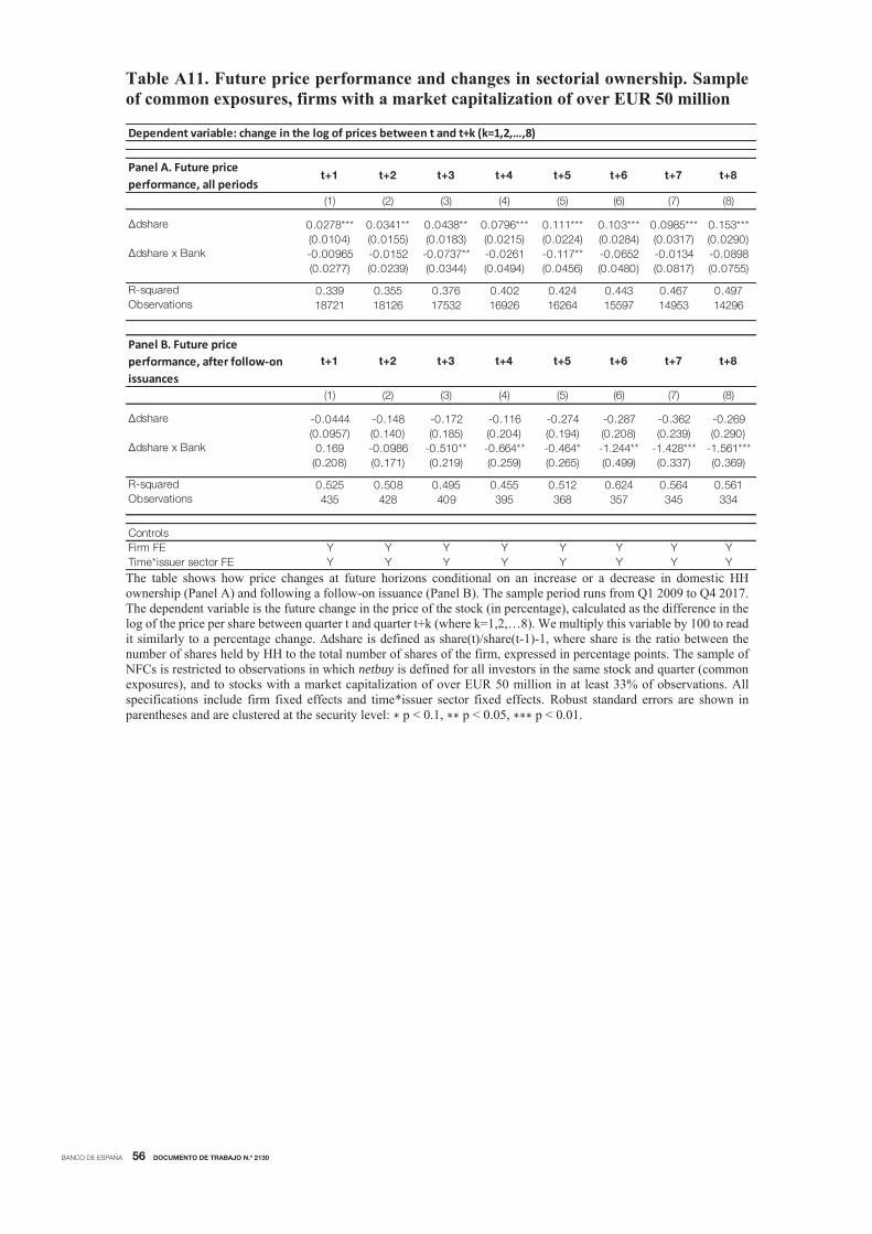
BANCO DE ESPAÑA 56 DOCUMENTO DE TRABAJO N.º 2130
Table A11. Future price performance and changes in sectorial ownership. Sample of common exposures, firms with a market capitalization of over EUR 50 million
The table shows how price changes at future horizons conditional on an increase or a decrease in domestic HH ownership (Panel A) and following a follow-on issuance (Panel B). The sample period runs from Q1 2009 to Q4 2017. The dependent variable is the future change in the price of the stock (in percentage), calculated as the difference in the log of the price per share between quarter t and quarter t+k (where k=1,2,…8). We multiply this variable by 100 to read it similarly to a percentage change. ∆dshare is defined as share(t)/share(t-1)-1, where share is the ratio between the number of shares held by HH to the total number of shares of the firm, expressed in percentage points. The sample of NFCs is restricted to observations in which netbuy is defined for all investors in the same stock and quarter (common exposures), and to stocks with a market capitalization of over EUR 50 million in at least 33% of observations. All specifications include firm fixed effects and time*issuer sector fixed effects. Robust standard errors are shown in parentheses and are clustered at the security level: p < 0.1, p < 0.05, p < 0.01.
Dependent variable: change in the log of prices between t and t+k (k=1,2,…,8)
Panel A. Future price performance, all periods
t+1 t+2 t+3 t+4 t+5 t+6 t+7 t+8
(1) (2) (3) (4) (5) (6) (7) (8)
∆dshare 0.0278*** 0.0341** 0.0438** 0.0796*** 0.111*** 0.103*** 0.0985*** 0.153***
(0.0104) (0.0155) (0.0183) (0.0215) (0.0224) (0.0284) (0.0317) (0.0290)∆dshare x Bank -0.00965 -0.0152 -0.0737** -0.0261 -0.117** -0.0652 -0.0134 -0.0898
(0.0277) (0.0239) (0.0344) (0.0494) (0.0456) (0.0480) (0.0817) (0.0755)
R-squared 0.339 0.355 0.376 0.402 0.424 0.443 0.467 0.497Observations 18721 18126 17532 16926 16264 15597 14953 14296
Panel B. Future price performance, after follow-on issuances
t+1 t+2 t+3 t+4 t+5 t+6 t+7 t+8
(1) (2) (3) (4) (5) (6) (7) (8)
∆dshare -0.0444 -0.148 -0.172 -0.116 -0.274 -0.287 -0.362 -0.269
(0.0957) (0.140) (0.185) (0.204) (0.194) (0.208) (0.239) (0.290)∆dshare x Bank 0.169 -0.0986 -0.510** -0.664** -0.464* -1.244** -1.428*** -1.561***
(0.208) (0.171) (0.219) (0.259) (0.265) (0.499) (0.337) (0.369)
R-squared 0.525 0.508 0.495 0.455 0.512 0.624 0.564 0.561Observations 435 428 409 395 368 357 345 334
Controls
Firm FE Y Y Y Y Y Y Y Y
Time*issuer sector FE Y Y Y Y Y Y Y Y

BANCO DE ESPAÑA PUBLICATIONS
WORKING PAPERS
2010 ALFREDO GARCÍA-HIERNAUX, MARÍA T. GONZÁLEZ-PÉREZ and DAVID E. GUERRERO: Eurozone prices: a tale of
convergence and divergence.
2011 ÁNGEL IVÁN MORENO BERNAL and CARLOS GONZÁLEZ PEDRAZ: Sentiment analysis of the Spanish Financial
Stability Report. (There is a Spanish version of this edition with the same number).
2012 MARIAM CAMARERO, MARÍA DOLORES GADEA-RIVAS, ANA GÓMEZ-LOSCOS and CECILIO TAMARIT: External
imbalances and recoveries.
2013 JESÚS FERNÁNDEZ-VILLAVERDE, SAMUEL HURTADO and GALO NUÑO: Financial frictions and the wealth distribution.
2014 RODRIGO BARBONE GONZALEZ, DMITRY KHAMETSHIN, JOSÉ-LUIS PEYDRÓ and ANDREA POLO: Hedger of last
resort: evidence from Brazilian FX interventions, local credit, and global fi nancial cycles.
2015 DANILO LEIVA-LEON, GABRIEL PEREZ-QUIROS and EYNO ROTS: Real-time weakness of the global economy: a fi rst
assessment of the coronavirus crisis.
2016 JAVIER ANDRÉS, ÓSCAR ARCE, JESÚS FERNÁNDEZ-VILLAVERDE and SAMUEL HURTADO: Deciphering the
macroeconomic effects of internal devaluations in a monetary union.
2017 JACOPO TIMINI, NICOLA CORTINOVIS and FERNANDO LÓPEZ VICENTE: The heterogeneous effects of trade
agreements with labor provisions.
2018 EDDIE GERBA and DANILO LEIVA-LEON: Macro-fi nancial interactions in a changing world.
2019 JAIME MARTÍNEZ-MARTÍN and ELENA RUSTICELLI: Keeping track of global trade in real time.
2020 VICTORIA IVASHINA, LUC LAEVEN and ENRIQUE MORAL-BENITO: Loan types and the bank lending channel.
2021 SERGIO MAYORDOMO, NICOLA PAVANINI and EMANUELE TARANTINO: The impact of alternative forms of bank
consolidation on credit supply and fi nancial stability.
2022 ALEX ARMAND, PEDRO CARNEIRO, FEDERICO TAGLIATI and YIMING XIA: Can subsidized employment tackle
long-term unemployment? Experimental evidence from North Macedonia.
2023 JACOPO TIMINI and FRANCESCA VIANI: A highway across the Atlantic? Trade and welfare effects of the
EU-Mercosur agreement.
2024 CORINNA GHIRELLI, JAVIER J. PÉREZ and ALBERTO URTASUN: Economic policy uncertainty in Latin America:
measurement using Spanish newspapers and economic spillovers.
2025 MAR DELGADO-TÉLLEZ, ESTHER GORDO, IVÁN KATARYNIUK and JAVIER J. PÉREZ: The decline in public
investment: “social dominance” or too-rigid fi scal rules?
2026 ELVIRA PRADES-ILLANES and PATROCINIO TELLO-CASAS: Spanish regions in Global Value Chains: How important?
How different?
2027 PABLO AGUILAR, CORINNA GHIRELLI, MATÍAS PACCE and ALBERTO URTASUN: Can news help measure economic
sentiment? An application in COVID-19 times.
2028 EDUARDO GUTIÉRREZ, ENRIQUE MORAL-BENITO, DANIEL OTO-PERALÍAS and ROBERTO RAMOS: The spatial
distribution of population in Spain: an anomaly in European perspective.
2029 PABLO BURRIEL, CRISTINA CHECHERITA-WESTPHAL, PASCAL JACQUINOT, MATTHIAS SCHÖN and NIKOLAI
STÄHLER: Economic consequences of high public debt: evidence from three large scale DSGE models.
2030 BEATRIZ GONZÁLEZ: Macroeconomics, Firm Dynamics and IPOs.
2031 BRINDUSA ANGHEL, NÚRIA RODRÍGUEZ-PLANAS and ANNA SANZ-DE-GALDEANO: Gender Equality and the Math
Gender Gap.
2032 ANDRÉS ALONSO and JOSÉ MANUEL CARBÓ: Machine learning in credit risk: measuring the dilemma between
prediction and supervisory cost.
2033 PILAR GARCÍA-PEREA, AITOR LACUESTA and PAU ROLDAN-BLANCO: Raising Markups to Survive: Small Spanish
Firms during the Great Recession.
2034 MÁXIMO CAMACHO, MATÍAS PACCE and GABRIEL PÉREZ-QUIRÓS: Spillover Effects in International Business
Cycles.
2035 ÁNGEL IVÁN MORENO and TERESA CAMINERO: Application of text mining to the analysis of climate-related disclosures.
2036 EFFROSYNI ADAMOPOULOU and ERNESTO VILLANUEVA: Wage determination and the bite of collective contracts in
Italy and Spain: evidence from the metal working industry.
2037 MIKEL BEDAYO, GABRIEL JIMÉNEZ, JOSÉ-LUIS PEYDRÓ and RAQUEL VEGAS: Screening and Loan Origination Time:
Lending Standards, Loan Defaults and Bank Failures.
2038 BRINDUSA ANGHEL, PILAR CUADRADO and FEDERICO TAGLIATI: Why cognitive test scores of Spanish adults are so
low? The role of schooling and socioeconomic background

2039 CHRISTOPH ALBERT, ANDREA CAGGESE and BEATRIZ GONZÁLEZ: The Short- and Long-run Employment Impact of
COVID-19 through the Effects of Real and Financial Shocks on New Firms.
2040 GABRIEL JIMÉNEZ, DAVID MARTÍNEZ-MIERA and JOSÉ-LUIS PEYDRÓ: Who Truly Bears (Bank) Taxes? Evidence from
Only Shifting Statutory Incidence.
2041 FELIX HOLUB, LAURA HOSPIDO and ULRICH J. WAGNER: Urban air pollution and sick leaves: evidence from social
security data.
2042 NÉLIDA DÍAZ SOBRINO, CORINNA GHIRELLI, SAMUEL HURTADO, JAVIER J. PÉREZ and ALBERTO URTASUN:
The narrative about the economy as a shadow forecast: an analysis using Banco de España quarterly reports.
2043 NEZIH GUNER, JAVIER LÓPEZ-SEGOVIA and ROBERTO RAMOS: Reforming the individual income tax in Spain.
2101 DARÍO SERRANO-PUENTE: Optimal progressivity of personal income tax: a general equilibrium evaluation for Spain.
2102 SANDRA GARCÍA-URIBE, HANNES MUELLER and CARLOS SANZ: Economic uncertainty and divisive politics: evidence
from the Dos Españas.
2103 IVÁN KATARYNIUK, VÍCTOR MORA-BAJÉN and JAVIER J. PÉREZ: EMU deepening and sovereign debt spreads: using
political space to achieve policy space.
2104 DARÍO SERRANO-PUENTE: Are we moving towards an energy-effi cient low-carbon economy? An input-output LMDI
decomposition of CO2 emissions for Spain and the EU28.
2105 ANDRÉS ALONSO and JOSÉ MANUEL CARBÓ: Understanding the performance of machine learning models to predict
credit default: a novel approach for supervisory evaluation.
2106 JAVIER ANDRÉS, ÓSCAR ARCE and PABLO BURRIEL: Market polarization and the Phillips curve.
2107 JUAN de LUCIO and JUAN S. MORA-SANGUINETTI: New dimensions of regulatory complexity and their economic cost.
An analysis using text mining.
2108 DANILO LEIVA-LEON and LUIS UZEDA: Endogenous time variation in vector autoregressions.
2109 CORINNA GHIRELLI, ANDREA GONZÁLEZ, JOSÉ LUIS HERRERA and SAMUEL HURTADO: Weather, mobility and the
evolution of the Covid-19 pandemic.
2110 KLODIANA ISTREFI, FLORENS ODENDAHL and GIULIA SESTIERI: Fed communication on fi nancial stability concerns
and monetary policy decisions: revelations from speeches.
2111 YUNUS AKSOY, HENRIQUE S. BASSO and CAROLYN ST AUBYN: Time Variation in Lifecycle Consumption and Income.
2112 JENNIFER PEÑA and ELVIRA PRADES: Price setting in Chile: micro evidence from consumer on-line prices during the
social outbreak and Covid-19.
2113 NEZIH GUNER, YULIYA A. KULIKOVA and ARNAU VALLADARES-ESTEBAN: Does the added worker effect matter?
2114 RODOLFO G. CAMPOS and JACOPO TIMINI: Unequal trade, unequal gains: the heterogeneous impact of MERCOSUR.
2115 JAVIER QUINTANA: Import competition, regional divergence, and the rise of the skilled city.
2116 PATRICK MACNAMARA, MYROSLAV PIDKUYKO and RAFFAELE ROSSI: Marginal Tax Changes with Risky
Investment.
2117 RODOLFO G. CAMPOS, JACOPO TIMINI and ELENA VIDAL: Structural gravity and trade agreements: does the
measurement of domestic trade matter?
2118 ALESSANDRO MELCARNE, JUAN S. MORA-SANGUINETTI and ROK SPRUK: Democracy, technocracy and
economic growth: evidence from 20 century Spain.
2119 ÁNGEL ESTRADA and DANIEL SANTABÁRBARA: Recycling carbon tax revenues in Spain. Environmental and
economic assessment of selected green reforms.
2120 ALEJANDRO FERNÁNDEZ-CEREZO, BEATRIZ GONZÁLEZ, MARIO IZQUIERDO and ENRIQUE MORAL-BENITO:
Firm-level heterogeneity in the impact of the COVID-19 pandemic.
2121 EDUARDO GUTIÉRREZ and CÉSAR MARTÍN MACHUCA: The effect of tariffs on Spanish goods exports.
2122 JACOPO TIMINI: Revisiting the ‘Cobden-Chevalier network’ trade and welfare effects.
2123 ALEJANDRO BUESA, JAVIER J. PÉREZ and DANIEL SANTABÁRBARA: Awareness of pandemics and the impact of
COVID-19.
2124 ALICIA AGUILAR and DIEGO TORRES: The impact of COVID-19 on analysts’ sentiment about the banking sector.
2125 SILVIA ALBRIZIO, IVÁN KATARYNIUK, LUIS MOLINA and JAN SCHÄFER: ECB euro liquidity lines.
2126 ANTHONY BALD, ERIC CHYN, JUSTINE HASTINGS and MARGARITA MACHELETT: The causal impact of removing
children from abusive and neglectful homes.
2127 IRMA ALONSO, PEDRO SERRANO and ANTONI VAELLO-SEBASTIÀ: The impact of heterogeneous unconventional
monetary policies on the expectations of market crashes.
2128 MARÍA T. GONZÁLEZ-PÉREZ: Lessons from estimating the average option-implied volatility term structure for the
Spanish banking sector.
2129 SIMÓN A. RELLA, YULIYA A. KULIKOVA, EMMANOUIL T. DERMITZAKIS and FYODOR A. KONDRASHOV: Rates of
SARS-COV-2 transmission and vaccination impact the fate of vaccine-resistant strains.
2130 MATÍAS LAMAS and DAVID MARTÍNEZ-MIERA: Sectorial holdings and stock prices: the household-bank nexus.