sectoral analysis - instructinstruct.uwo.ca/economics/221b-570/2221bignotes.doc · web...

Macroeconomics 157 Ch VI. Consumption

Sectoral Analysis

Chapter VI. Consumption Function

1. Keynesian Theory

1) Background

We have learned that the Keynesian consumption function in general takes the form

where C0 is the basic consumption, c1 the marginal propensity to consume, and Yd the disposable income which is equal to income minus taxes. Implicit herein is the assumption that changes in income and changes in consumption are contemporaneous.

So by introducing time subscript, we can rewrite the above as

Keynesian economists estimated consumption function by obtaining a best fitting line with time-series data of disposable income and consumption.

For instance, with the U.S. yearly data of the period 1929-1941, the consumption function for the whole U.S. economy was estimated as

Ct = 47.6 +0.73 Ydt

(unit: in 1972 Billion U.S. dollars);

With the Canadian yearly data of 1926-1940, the consumption function for Canada was estimated as

Ct = 3.0 + 0.69 Ydt (in 1972 Billion Canadian dollars).

So we can make a prediction as to the magnitude of consumption if we have a reasonable forecast about income. Alternatively, as we have seen in the above


Question #1, we can get the value of the APC for a predicted level of national disposable income

Question #1: Suppose we have obtained the consumption function in Question #1 from the past data. What is the APC for a personal disposable income of $ 150 billions in 1972 dollars? The answer is 0.71; the consumption is 3.0 + 0.69 times 150 from the equation, and is equal to 106.5. The APC is this consumption $ 106.5 billions divided by the total disposable income $ 150 billions.

Question #2: Suppose we have obtained the consumption function in Question #1 from the past data. What is the APC for an personal disposable income of $ 200 billions in 1972 dollars? The answer is 0.705; the consumption is 3.0 + 0.69 times 200 from the equation, and is equal to 141. The APC is this consumption $141 biiions divided by the total disposable income $ 150 billions.

2) Implications of Keynesian Consumption Model

Two corollaries we can draw from the above equation are

Average Propensity to Consume (APC) is larger than Marginal Propensity to Consume (MPC); more importantly, the APC decreases as income increases. This implies a non-proportionality between an increase in income and the responsive increase in consumption. As income rises, a smaller and smaller portion of income will be spent as consumption. The above questions #1 and 2 illustrate the APC falls as income increases.

The estimation of the Marginal Propensity to Consume (MPC) enables government policy makers to compute the multiplier and thus to know exactly how much government expenditures or taxes should be adjusted in order to increase the national income by the target amount.

Quite important implications behind the two points are as follows:

The first point is a terrible prognosis for a growing economy. The APC shows the proportion of the total income to be consumed. A small APC means a small portion of income to be transformed into expenditures.Savings are, in the circular flow model of the Keynesian theory, a leakage, which lowers the Aggregate Expenditures and subsequently the level of the national income in the next round. As the APC decreases in a growing economy, an increasingly larger proportion of income is saved away and thus there occurs a deficiency of aggregate expenditures. The aggregate output continues to grow while the aggregate expenditures stagnate due to an increasingly larger proportion of income to be saved away. The result is a secular stagnation. This implication that a growing economy will be inevitably faced with Secular Stagnation due to a deficiency of


aggregate expenditure or an excessive saving is in line with Marxists' argument that the capitalist economy is bound for general glut due to excessive savings by stingy capitalists.

In the Keynesian view, the second point is a miracle cure for the problem of a falling APC: By using the multiplier government may know exactly how much it has to supplement the aggregate expenditure which is not sufficient if left to the private sector.

3) Keynesian Justification

The Keynesian Proof of the first point of a declining APC in the face of a growing income is as follows:

By definition, in general, the marginal propensity to consume (MPC) is the ratio of the responsive increase in consumption to a unit increase in income. It measures what proportion of an incremental increase in income is consumed. The average propensity to consume (APC) is the ratio of the total consumption to the total income. It measures what proportion of the total income is consumed.

(1) Illustration

Graphically, the MPC is the slope of the consumption curve and is constant over the entire range of income.

The APC measured at a certain level of income is the slope of the ray which links the origin and the corresponding point on the consumption curve.

0

R1 R2


At Y1, MPC = c1; APC = Slope of the OR1 ray.

At Y2, MPC = c1; APC = Slope of the OR2 ray.

(Note: the OR1 is steeper than the OR2, and therefore; APC at Y1 >> APC at Y2.)

Algebraically, we can also show that

As Ct = C1 + c2 Ydt,

So the APC is the MPC plus a positive term. And thus APC - MPC = C0/Ydt which is positive. Therefore, APC >> MPC.

We note that the term C0/Ydt is a decreasing function of income level; the numerator C0

is constant regardless of the level of Yd. As Yd increases in the denominator, the ratio falls.

Therefore, the APC falls as income increases. A smaller and smaller proportion of income will be spent and thus be transformed into the aggregate expenditures. This means that the average propensity to save rises as income increases.

Ydt = Ct + St

Dividing the both sides of the above equation by Ydt, we get

As the income is increasing, the APC is falling and the APS is rising.

(2) Numerical Example

The consumption equation (unit: in 1971 Billion dollars) is given as

Ct = 3.0 + 0.69 Ydt.

What is the MPC?


What is the APS at Ydt = $ 150 billion? What is the APS at Ydt = $ 200 billion?

These feature, i) "dAPC/dYd < 0" or the APC falls as income increases, and ii) "APC > MPC", basically the same results from the fact that the consumption function has an intercept.

If the consumption function is a ray from the origin and thus without any intercept, the APC will be equal to the MPC and the APC would be constant all the time just like the MPC. The APS will be constant over the entire range of income. As income rises, the increase in consumption is proportional to the increase in income.

4) Two Empirical Anomalies

Upon the Keynesian theory, economists who have been working on historical data have found two empirical anomalies:

1) "The estimated consumption function underpredicted the consumption for a higher level of income";

For instance, income has grown over time after World War II. We have seen that by substituting the forecasted level of national income into the estimated consumption function, we can get the predicted value of consumption and thus the APC. Economists did so in the pre-war time for the post-war era. Over time it was revealed that the consumption level predicted in the pre-war time for the post-war era was smaller than the actual post-war consumption. Also the predicted APC turned out to be smaller than the actual APC. For instance, when we predict the APC for the disposal national income level of $150 billions, it is about 0.71. However, historically, when the actual income was equal to $150 billions in Canada, the actual APC was about 0.85 rather than 0.71.

A few possibilities;

The first one is people have become more prodigal in the post-war period. The MPC might have increased in the post-war period compared to the MPC of the pre-war period. And thus the APC might have increased over time, too.

The second possible scenario is that the average and marginal propensities might have been wrongly measured in the estimation process. And there might have been a systematic error in estimating consumption.

If the first is true of the two possibilities, the Keynesian consumption function would be preserved, and there would be no further need for research geared to improving economic theory. This is an academically uninteresting case.

2) "The long-term APC thus APS were constant over a long period of time"


Professor Simon Kuznets estimated the long-run APC by observing the changes in consumption and income during a considerable long period of 1869 to 1933, and found that the long-run APC was constant at 0.89 over time. This result contrasts with the estimation result from a relatively short-period data.

This implies that there are two kinds of consumption curve, short-term and long-term:

The long-run consumption curve can be drawn as a ray from the origin;

There, long-run APC = long-run MPC as there is no intercept; the APC and APS are constant over the entire range of income.

long-run MPC >> short-run MPC if the short-run consumption curve is based on the yearly changes in income as shown above.

In attempts to resolve these anomalies, some alternative hypotheses about the consumption behaviour were proposed. These alternative consumption theories differ in the length of the time-horizon over which consumers are assumed to make consumption decision.

2. Permanent Income Hypothesis

1) Basic Ideas

M. Friedman says that the current consumption is a function of permanent income Yp.

Permanent income is a sort of income stable in the long run. Its calculation requires an observation over multiple periods of time. ctrue is a true value of marginal propensity to consume measured out of permanent income. This contrasts with c1 or the simple and conventional Keynesian type of marginal propensity to consume measured out of current income.

2) Fictitious Keynesian Consumption Function

He argues that in order to get the correct consumption function we should lengthen the period of observation, or should observe income and consumption for a sufficiently long time. Trying to attribute changes in current consumption to changes in current income would lead to a fictitious or erroneous consumption function.

The following example will be helpful in your understanding his point;


For instance, suppose that in an economy all the people are identical and homogeneous who are all paid $ 110 per week. The only inter-personal difference is that the one sixth of workers are paid on each day of the weekdays. So 1/6 are paid on Monday, another 1/6 on Tuesday, and so on... Let suppose that the workers spend more, say $ 40, on the pay day, than on other days of the week, say $10 per day. So they save $ 10 each week.

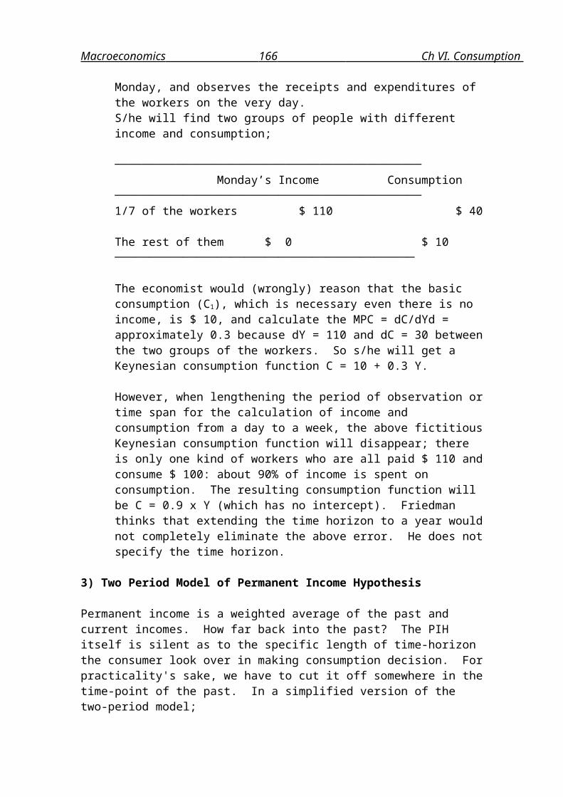
A Keynesian economist would like to examine the relationship between current income and current consumption. And s/he chooses a day of the week, say, Monday, and observes the receipts and expenditures of the workers on the very day.S/he will find two groups of people with different income and consumption;

─────────────────────────────────────────────Monday’s Income Consumption

─────────────────────────────────────────────1/7 of the workers $ 110 $ 40The rest of them $ 0 $ 10────────────────────────────────────────────

The economist would (wrongly) reason that the basic consumption (C1), which is necessary even there is no income, is $ 10, and calculate the MPC = dC/dYd = approximately 0.3 because dY = 110 and dC = 30 between the two groups of the workers. So s/he will get a Keynesian consumption function C = 10 + 0.3 Y.

However, when lengthening the period of observation or time span for the calculation of income and consumption from a day to a week, the above fictitious Keynesian consumption function will disappear; there is only one kind of workers who are all paid $ 110 and consume $ 100: about 90% of income is spent on consumption. The resulting consumption function will be C = 0.9 x Y (which has no intercept). Friedman thinks that extending the time horizon to a year would not completely eliminate the above error. He does not specify the time horizon.

3) Two Period Model of Permanent Income Hypothesis

Permanent income is a weighted average of the past and current incomes. How far back into the past? The PIH itself is silent as to the specific length of time-horizon the consumer look over in making consumption decision. For practicality's sake, we have to cut it off somewhere in the time-point of the past. In a simplified version of the two-period model;


where θ is in the range between zero and one, and indicates the extent to which people regard the current increase in income as permanent.

For instance, people assign 1 to θ when they regard the entire increase in income as permanent or persisting in the future. Then all the change in the current income will become the change in permanent income, and the c1 (=MPC) fraction of the increase in permanent income will translate into a change in consumption.

However, they will assign 0 to θ when they regard the entire increase in income as transitory or temporary. The increase in current income will not affect the permanent income, and therefore there would not be any change in consumption.

What is the MPC? There are multiple MPC's depending on what income to use in measuring the MPC.

When the MPC is measured against the permanent income: MPC measured out of permanent income = dCt /dYp .

Differentiating both sides of equation (1) with respect to Yp, we get

dCt / dY p = c ture.

The MPC measured out of current income (Yt) = c1= dCt / dYt;

Substituting equation (2) into equation (1), we get

Differentiating the above equation with respect to Yt, we can get

c1 = d C t/dYt = ctrue θ.

Obviously, ctrue > ctrue θ, because 1 > θ and thus cture x 1 > ctrue x θ.

The larger θ is, the larger the impact of changes in current income on permanent income and consumption;

(1) When θ is equal to one, the MPC measured out of permanent income will be just equal to the MPC as is the case of the Simple Keynesian consumption function.


(2) When θ is equal to zero, the MPC measure out of permanent income will be zero because there is no change in permanent income and thus no change in consumption. The increase in income will be mostly saved, and thus the ratio of saving to income will rise.

(3) Usually 0 < θ < 1. The MPC is measured out of.

Historical Evidence that a transitory increase in income or windfall of income does not increase consumption very much.

(1) There was a one-time restitution payment from Germany to the Israeli citizens. The payment was equal to the average annual income per household. Only 20 % of the amount received was spent out as consumption.

(2) In 1950, there was a unanticipated, one-time payment of life insurance dividends to the U.S. Word War Two veterans. It was $ 175, which amounted to 4 % of annual household income. Consumption rose only by 1 % that year (less than 30 % of the windfall increase in income was spent).

3) Life Cycle Hypothesis

Life Cycle Hypothesis specifies (1) the time horizon, which the consumer consider in making consumption decision, as her/his life time, and (2) include wealth in the income and thereby regarding wealth as making differences in consumption for a given level of labor income.

(1) A consumer's time horizon is equal to her/his life time;

the consumer will first figure out the total amount of resources available for consumption during his/her entire life time. This total amount of resources available during the life time is called 'Life-time Budget Constraint', which is specified, assuming life span is 75 years, as

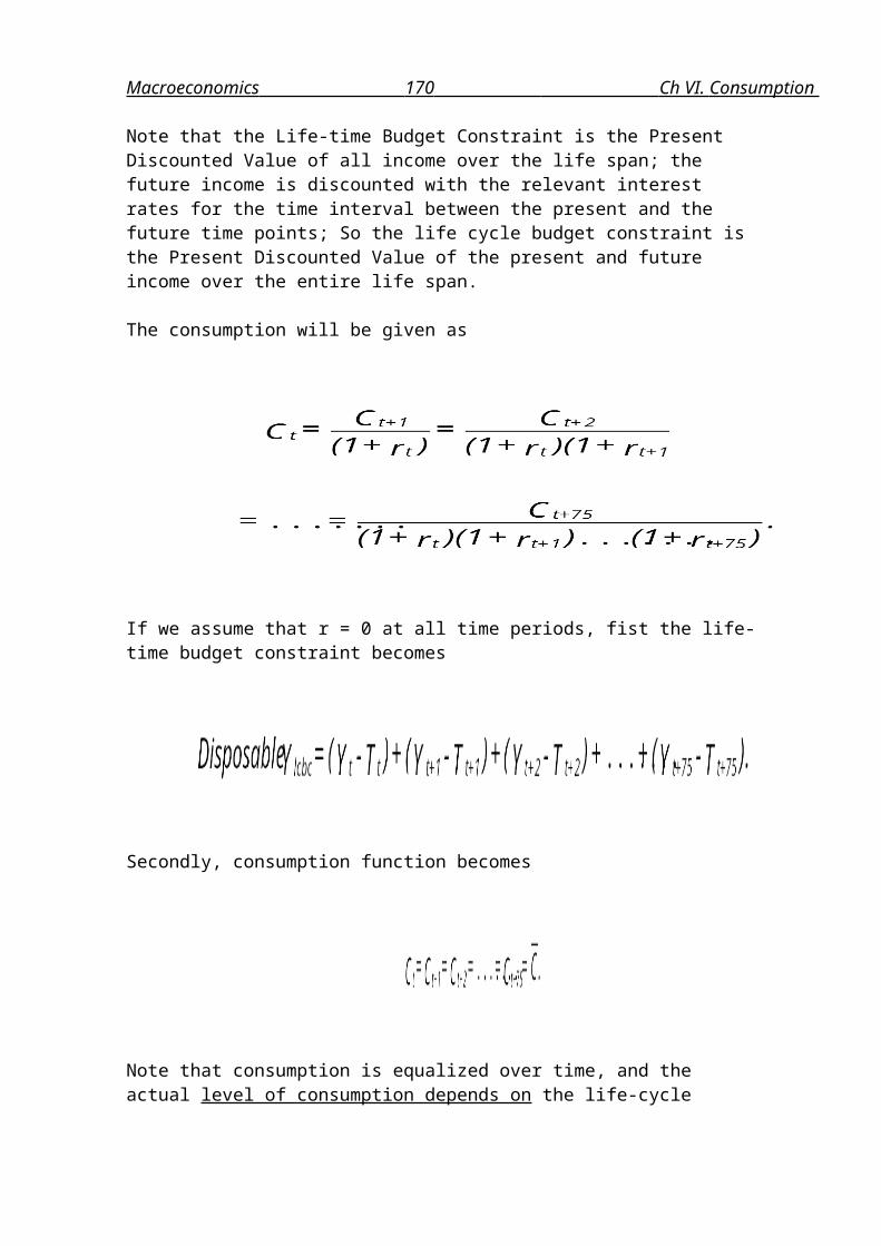
Note that the Life-time Budget Constraint is the Present Discounted Value of all income over the life span; the future income is discounted with the relevant interest rates for the time interval between the present and the future time points; So the life cycle budget


constraint is the Present Discounted Value of the present and future income over the entire life span.

The consumption will be given as

If we assume that r = 0 at all time periods, fist the life-time budget constraint becomes

Secondly, consumption function becomes

Note that consumption is equalized over time, and the actual level of consumption depends on the life-cycle budget constraint which in turn is a function of the current and future income over life time. Broadly speaking consumption function is given as

Let us examine some implicit assumptions behind this life-cycle hypothesis before making more realistic modifications to them;


(1) There is No Uncertainty. The L.C.H. assumes perfect foresight for the consumer; s/he is assumed to know the entire profile of current and future incomes. When s/he is born at time t, s/he knows what the current and future personal disposable incomes are and what the current and future taxes are. Government is acting along a preannounce path of policies.

(2) The preference of the consumer is that s/he can maximize her/his utility over time by smoothing the consumption profile or by spreading consumption evenly over time.

The equal amount of consumption for each period will maximize the total utility, because of the decreasing marginal utility of consumption.

Here a tax cut or decrease in tax (dTt+25), say, at time t+25, does bring about no increase in consumption at time t+25 compared to that at time t+24 or dCt+25 = Ct+25 - Ct+24. It means dCt+25/dTt+25=0. That is because the tax cut was already correctly and completely predicted and thus consumption was already adjusted (at time t or at the beginning).

(2) Wealth matters;

Consumption is a function of life-time labor income and wealth;

Ct = c YL + a WL, where

YL is the (life-time) labor income and WL wealth.

For a given level of labor income, at a personal level, the larger wealth one has, the larger APC will be when it is measured against (conventional labor) income;

Ct/Yt = c YL/Yt + a WL/Yt.

4) Modern Frontier Consumption Theory

(1) In the real economy, there is uncertainty to the future. The best one can do is to make an educated guess, or to form expectations by efficiently utilizing information contained in 'news'.

Now consumption depends on the current and all the expected future incomes during the life time; A revision of expectations provoked by the receipt of news about the occurrence of shock or unanticipated events involving future disposable income will


lead to changes in consumption; the modified Life Cycle Model in the presence of uncertainty will be

where * means expected future variables.

Example:

For instance, government may suddenly announce at time t that it will decrease tax at time t+25. This comes as surprise or shock as it was an unanticipated, unforeseen, unpredicted event. The 'news' leads to the revision of the expectations of the future income (Tt+25

*). Therefore, the Expected Life-cycle Budget Constraint will be revised upward at time t, and accordingly consumption level will be raised once-and-for-all at time t.

When actually the tax is raised at time t+25, nothing is out of blue. The event has been fully anticipated, and perhaps by this time all the necessary adjustments have been made. Thus the tax cut at t+25 would not bring about any adjustment in consumption at time t+25.

The changes in tax and consumption are not contemporaneous any more; at time t, consumption changes even if there is no change in tax or current disposable income. At time t+25, there will be no change in consumption while there occurs changes in disposable income due to the tax cut. Probably, by now, all the necessary adjustments have been made in response to this fully anticipated tax cut.

(2) The time-horizon may extend beyond life-time if the consumer cared about the welfare of her/his descendant(s), and so on for each subsequent generation.

Suppose there is a tax cut at time t+25, and the decrease in government revenue due to the tax cut will be offset by an increase in the revenues from issues of bonds. As the bonds have maturity and should be retired sometime in the future. Let us also suppose that government is planning to retire these bonds by increasing tax at the year t+76, a year after the death of a particular consumer. Within the framework of L.C.M. which regards the time horizon of a consumer as being limited to her/his life time, the consumer can enjoy the benefit of tax cut and avoid the future tax-liability (s/he dies at the year t+25). So the tax cut will be regarded as bonanza or windfall gains and lead to increases in consumption.

However, it s/he cares about the future generation, s/he will give weight to the disposable income and expenses of the future generation. In the above case, s/he


would like to lessen the future tax liability to be imposed upon her/his children. So s/he will save the benefits from tax cut by buying bonds newly issued, and bequeath bonds to the descendant. At the year t+76, the descendants will cash the bonds and pay the increase in tax-liability which is necessitated for the repayment of government debts. In this case, all the government does is to move tax over the time horizon, and thus to delay taxation. That kind of `intertemporal reallocation of taxation' does not alter the total amount of resources available for a consumer. The consumer will not change her/his consumption behaviour. Therefore there is no further impact on economy. So the Ricardian Equivalence holds (which says that switching from one method of financing to another does not matter, or that deficit-financed and tax-financed government fiscal policies are equivalent, unlike the Keynesian argument that there is no equivalence between the two because the former is more effective with the associated multiplier (=1/{1-c}) having a larger magnitude than the latter with the corresponding multiplier which is equal to one). Here the consumer acts as if s/he would live an infinite life. The inter-generational link is the bequest (motive).

Now in the infinite time horizon model, a general form of consumption function should be again modified as a function of income and tax variables of the current and all the future time points up to the infinity;

(3) Liquidity Constraint

L.C.H. assumes that the consumer can completely smooth the consumption profile by effectively financing current consumption with future income. This is possible when one has an unconstrained access to credit market, and thus can borrow or lend freely.

In reality, a lot of people have only limited access to credit market. Particularly this is the case for those who have wealth in the form of human capital. For instance, most people agree that students will earn more income in the future. But risk-averse people will not give unlimited credit to students. The students are faced with liquidity constraint and their consumption is below the desired level. When the liquidity constraint is lifted up, there will be increase in consumption because the previous consumption is somehow suppressed.

Application:Consumption Function and Tax Cut (Fiscal Policy)


Why does the specification of consumption function make difference in fiscal policy implications?

The consumption function is important because it characterizes a most important link within the mechanism of fiscal policy.

Once a renowned economist Professor Edmund Phelps asked in the class, “What is the ultimate purpose of tax?". The answer is that through Taxation and consequent changes in disposable income the government can affect Consumption. Changes in consumption, which is the largest component in the Autonomous Expenditure or YD, will bring about changes in equilibrium national income. So the sequence of fiscal policy involving tax cut is that dT (changes in T) dPDI dC dYD = dAE dYe.

It can be explained in the following details;

The tax multiplier or dYe/dT can be broken into the chain of functional relationships such as

Note that the first component is the multiplier which is equal to 1/{1-c1}. The second one is always one because YD = C + I + G; C will increase YD at the one dollar-to-one dollar ratio. The third is the MPC whose magnitude depends on the specification of consumption function. The last component dPDI/dT = d(Y-T)/dT is one in the Keynesian consumption theory, while in the PIH dPDI/dT = dYp/dT = θ.

The purpose of this chapter is that depending on the link dC/dPDI and dPDI/dT, the impact of tax cut on national income is not that simple, and varies much. We will examine how the modification of the simple Keynesian consumption function could alter the implications of fiscal policy, particularly tax-cut.

2) Permanent Income Hypothesis

In the context of the PIH, the tax multiplier which indicated the impact of tax cut on equilibrium national income can be broken into


We can show the following:

At equilibrium YS = YD, where YS = Y and YD is as given as above,

The PIH suggests that the tax cut will shift the IS curve only by the θ fraction of the distance of shift of IS as is suggested by the Keynesian model.


3) Life-cycle Income Hypothesis

We know that the present tax cut leads to budget deficit at the margin, and necessitates the issue of bond. The crucial point is when the bond will have to be retired sometime in the future, and that this retirement will be done by a tax increase. So basically all the government does in cutting tax is to delay tax over time. The crucial matter for the consumer is whether the bond will be retired and at the same time tax will be increased for that purpose; if the present tax cut has a tax increase within the life time, the consumer knows that s/he cannot escape the future tax liability and thus will not regard the present tax-cut as `free lunch.' S/he saves the increase in income which results from the decrease in tax by buying bonds, and will keep them until the tax raise. Then s/he will cash the bonds and pay the increased tax. In this way her/his consumption is kept smooth, and needs not be swayed by the whimsical government policies against her/his preferences.

4) Modern Frontier Consumption Function

(1) If the L.C.H is true and correct, and if the government will correct the future tax after her/his death, then the present tax cut is regarded as `free lunch,' whose bill will have to be picked up by the future generation s/he does not care about. Her/his consumption will increase upon the news that there will be a tax cut. So in this case of finite time-horizon model, the Ricardian Equivalence fails to hold.

If the time horizon is infinite because a generation cares about its subsequent generation, the consumer will behave as if s/he lives an infinite life; s/he equally weighs the present tax cut and the future tax liability. S/he will save the benefit from the present tax cut and bequeath the saving to the future generation or ‘bequest’, which will be cashed to pay the (future) tax liability, which originated from the tax cut. The bequest motive is the operational link between generations.

(2) Rational expectations theory says that in the real world with uncertainty, consumption is a function of the current and all expected future incomes. Therefore expectations about the future affect current consumption behaviour. Whenever there is a revision of expectations about the future, which is prompted by the receipt of news about unanticipated event, there will be changes in consumption.

Anticipated changes in income, or fully foreseen tax cuts would not bring out any concurrent changes in consumption, when actually the tax cuts happen. Because the tax cuts were fully anticipated in the past and were acted upon it at that time of perception, by the time when actually the even occurs, all actions have been taken and no further actions will be left to be taken.

In summary, only unanticipated shocks will bring about changes in consumption, and therefore the changes in consumption will be unpredictable or 'random walk.'


Example: There is no actual tax cut now at time t. But there is 'news' about the future tax cut of time period t+5. The consumer will revise expectations about the future income upward. The extent to which s/he revises expectations also depends upon her/his judgement as to whether the tax cut is permanent or temporary, or in other words, whether it is for one period or for multiple periods. As her/his expected future income increases, her/his consumption will increase now at time t. At time t+5 when actually the fully anticipated tax cut happens, there would not be any change in consumption.

Macroeconomics 174 Ch VII. I nvestment

Chapter VII. Investment Function

1. Definition

Investment consists of

Fixed Capital Investment: Machinery, Equipment, Non-residential Building, and Residential Construction Addition to Inventory: finished goods and materials on the pipeline, and

also buffer stock of finished goods.

We can also divide the total or gross investment into replacement investment or capital consumption allowances and net investment;

Gross Investment = Net Investment + Depreciation

There are suggestions to include Consumer Expenditures for Durables in Investment.

2. Biggest Issue: Volatility of Investment

Investment is much more volatile than income or consumption; Inventory Investment is still more volatile.

3. Explanations for Volatility of Investment.

1) Keynesian Accelerator Model of Investment

(1) Model

Inverting the following Aggregate Production Function with labor input being held constant

we can rewrite the above equation into;


We can also apply this to the last period;

Investment is the increase in capital stock which is proportional to the increase in (the production of aggregate output, which is equal to) national income;

Differentiating both sides with respect to time t, we get

The rate of change in investment depends on the acceleration/deceleration of the growth rate of income, or the change in the rate of change in income.

(2) Numerical Example:

Assumption: Ct = 50 + 0.8 Yt, It = 3 (Yt - Yt-1). Note that v =3 here.

────────────────────────────────────────────────── Year Yt % change Ct % change Kt It % change────────────────────────────────────────────────── 1 450 410 1350 2 500 11 % 450 10 % 1500 150 3 600 20 % 530 17 % 1800 300 100 % 4 660 10 % 580 9.5% 1980 180 -40 % 5 726 10 % 630 8.6% 2178 190 5 %─────────────────────────────────────────────────

Note that the % change in income and the % change in consumption go hand in hand in a similar proportion. However, the % changes in investment are much more volatile than those in national income or consumption.

In fact it is in a proportion to the % change of the % change in income; the % change in the % change in Y between years 2 and 3 (from 11% to 20%) is 82%. The % change in


the % change in Y between years 3 and 4 (from 20% to 10%) is -50%. The % change for the subsequent period is 0%. These numbers, 82%, -50%, and 0%, are in line with the % changes in investment, 100%, -40%, and 5%.

Therefore,

Acceleration in Y (an increase in the growth rate of national income) I

Deceleration in Y (a slow-down of the growth rate) I

Whether investment will increase or decrease this year in comparison to the last year's investment depends on whether the growth rate of this year is larger or smaller than the growth rate of the last year;

For instance, suppose that the real income grew 3% last year, and grows 1% this year. The economy is still growing; income increases this year and so does the consumption. But the investment will decrease compared to the last year's level because the growth rate drops from 3 to 1 % or the growth decelerates.

(3) Implications of the Keynesian Accelerator Model;

i) When the above investment function as a function of changes in income is substituted in the equilibrium national income equation, the only exogenous variables left over are autonomous consumption (C) and government expenditure (G). So what ultimately determines the equilibrium national income is G.

ii) Substituting the above investment function into the equilibrium income function, we get a first-order difference equation; Yt = A (G + C) + B Yt-1. Depending on the value of B, there could be different patterns of business cycles.

(4) Problems

i) This is a circular argument; Y changes as I changes, which changes as Y changes. Therefore this is rather a mechanical illustration than a explanation which touches the fundamental causes of volatility of investment.

ii) There is some factor which attenuates the volatility of investment; the adjustment cost makes actual fixed capital, investment or increases in fixed capital, take place over time in a gradual fashion rather than over night. But the adjustment cost is minimal for inventory investment.


The actual change in capital stock or dK cannot take place overnight. The time lag involved in increasing K is fairly long (think about the construction period, and the time lag between the order and the shipment of equipment and machinery). Inventory Investment does not involve any significant lag.

2) Neoclassical Model of Investment

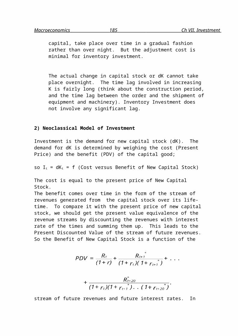
Investment is the demand for new capital stock (dK). The demand for dK is determined by weighing the cost (Present Price) and the benefit (PDV) of the capital good;

so It = dKt = f (Cost versus Benefit of New Capital Stock)

The cost is equal to the present price of New Capital Stock.The benefit comes over time in the form of the stream of revenues generated from the capital stock over its life-time. To compare it with the present price of new capital stock, we should get the present value equivalence of the revenue streams by discounting the revenues with interest rate of the times and summing them up. This leads to the Present Discounted Value of the stream of future revenues. So the Benefit of New Capital Stock is a function of the stream of future revenues and future interest rates. In reality where there is uncertainty, the future values are unknown. The best the investor can do is to make a rational guess about the future variables. This means that the PDV becomes the function of expected future variables such as expected future revenues and expected future interest rates;

where * denotes expected future variables, Rt+i is the stream of revenues from the investment project, r interest rate.

The revenue is the value of sales of output (= the price of output multiplied by the amount of output demanded and thus produced) minus tax, and so on;


Implications:

(1) There are a lot more expected variables in the investment function than in any other function; the expectations matter more in the investment function than in other functions.

(2) The expectations change all the time, reacting to 'News', which may not be necessarily correct.

(3) Among the expected variables which affect the PDV of the investment project, in percentage terms, the interest rate is the most volatile. For instance, at the aggregate level, revenues rarely change by 50% (due to such changes in sales or price) while the interest rate often changes by 50 % (from the 11 % to 15 % level or the other way around). So ultimately, a substantial part of the volatility of investment can be explained by the volatility of interest rate. What makes interest rate volatile? It should be considered in the context of Money Supply and Demand. Naturally this has a lot to do with the next topic of this course.

3) Rental Cost of Capital

Investment is the demand for new capital stock or an increase in capital stock(ΔK). The demand for ΔK is determined by weighing the cost and the benefit (or revenue) of the capital good at the margin.

Marginal Revenue = Marginal Cost.

Let's suppose that you are an investor or entrepreneur. You are borrowing money from a bank at the interest rate of i for a year and buy a capital good. You produce outputs from the use of the capital good, and sell it in a year to repay your loan from the bank.

Your revenues come from two sources: During the year, there will be product generated from the machine. At the end of year when you sell the machine you will have gains or loss as the price of the machine has changed.

The marginal revenue is the sum of the marginal product of capital MPK (for a year) and the capital gains or loss due to the changes in price of the capital good (when you are selling your company at the end of a year):


You incur two kinds of cost: one is the interest ("i") you pay to the bank. The other is that the machine needs repairs, that is, depreciation. Let's suppose that with the payment for depreciation the machine is maintained in as good a condition as a new one:

Here the interest rate i is determined in the money market. The percentage change in the price of the capital good may be in line with the rise of the general price level:

MPK is primarily a decreasing function of capital stock. It is also an increasing function of technical innovation and a decreasing function of any event which adversely affects productivity of capital (for instance, oil shocks).

By transposing the rate of inflation, we rewrite the equilibrium condition as follows:

We call the right-hand side express the user (rental) cost of capital.

Note that the interest rate minus the rate of inflation is the real interest rate. Therefore, the equilibrium condition is that the marginal product of capital is equalized with the user cost of capital, the sum of the real interest rate and the depreciation rate.

Applications of Rental Cost of Capital Model: How does this model work in respond to variety of changes?

For some reason of external shocks (such as an increase in real interest rate) the MC may rise. To ensure the equality between the user cost and the MPK, the MPK should rise to re-establish the equality. MPK will rise when K decreases. Investment should decrease. Intuitive explanation is that when the user cost of capital rises, the least productive project of investment should go to enhance the marginal productivity of capital of the existing project. We will observe that


the negative correlation between the interest rate and investment: An increase in the real interest rate will lead to a decrease in investment.

For some reason (such as oil shocks, which lead to cumbersome and disruptive energy saving measures) the MPK may decrease. The two forces will start working. In order to re-establish the equality, the MPK of the left-hand side should rise back. The capital stock should decrease to have an increase in MPK. The least productive project should go to enhance the productivity of capital. This decrease in the demand for capital will lead to a fall in the interest rate or th lending rate of the bank. In the right-hand side of the equality, the real interest starts falling. We will observe a positive correlation between the interest rate and investment.

A decrease in the nominal interest rate will not necessarily lead to an increase in investment; For instance, in 1990, the nominal interest rate was about 12% and the rate of inflation stood around 7%. The user cost of capital was then 12 minus 7 % plus depreciation rate. Now the nominal interest rate is only 8%, and the inflation rate is 2%. The current user cost of capital is 8 minus 2 % plus depreciation rate. The current user cost is higher than that of 1990. What matters to the investor is not the nominal but the real interest rate.

4) Tobin's Q Theory

According to James Tobin, the `Q' index larger than one is a green-light signal for expansion of facilities or new investment. The Q index is equal to the market value of a firm over the replacement cost of a firm: The market price incorporates the market’s expectations as to the prospect of future business returns to the firm, while the replacement cost is simply the present market price of capital required to set up the firm.

Tobin's Q shows how or through what transmission mechanism, for instance, an increase in money supply leads to an increase in investment. If money supply increases, other things being equal, expenditures on all assets will rise. As the demand for stocks rises, the stock prices will go up. The market value of a firm is the stock volume times the stock price. As the market value of stocks rises, Tobin's Q exceeds one. There occurs a new physical investment.

5) Permanent versus Temporary Investment Tax Credits?

By nature, investment can be done in the discrete manner; investment spurts, making the best use of an auspicious investment environment, which comes occasionally ("Make hay while the sun shines").

Implication: A temporary tax cut on investment will have a larger expansionary impact on investment than a permanent tax cut. This contrasted with the case of tax cut on


income; a permanent income-tax cut has a larger impact on consumption and aggregate expenditures than a temporary income-tax cut.

"....... Congress may revive the investment tax credit (ITC) in hopes of boosting spending on factories and equipment. Bush would probably sign on. Experts caution that ITC would be truly helpful only if the credit is temporary...." (The Times, "Does America Need a New Deal for the Nineties?", January 13, 1992).

Macroeconomics 182 Ch VIIII. O pen Macroeconomics

Chapter VIII. Money

We have already learned that the LM curve shows the combinations of interest rate and income (i, Y), which satisfy the equilibrium in the money market. It comes from the money supply and demand curves: The equilibrium in the money market, that is, the money supply being equal to the money demand, yields the interest rate.

1. Nominal versus Real Quantity of Money

In economics we define the demand and supply in real terms, not in nominal terms. It is in line with the microeconomics expression of demand and supply. Let's take an example of the demand and supply of hamburgers. We say that 5000 units of hamburgers are demanded at the price of $4. If we say that $20,000 worth of hamburgers are demanded, the statement is not clear enough. If the price is $1, 20,000 units of hamburgers are demanded in real terms. If the price is $10, the demand for hamburgers in real terms is 2,000 units. We can dispel any ambiguity by expressing the volume of demand and supply in real terms- here `real' means no change in response to changes in prices. The nominal quantity of money (supply or demand) is the face value of the total amount of money, and the real quantity of money is the face value divided by price level;

Real quantity of money = Nominal quantity of money / Price level:

m = M/P

At the equilibrium in the money market, the money supply in real terms is equal to the money demand in real terms:

ms = md.

Nothing further will happen to national income, interest rate, and so forth. At disequilibrium, there occurs an excess supply of or demand for money. The equilibrating forces come in to push back the economy to the equilibrium. In this process there occur changes in such variables as income, and interest rate.

It is of great importance to understand the operation of the above equation describing the equilibrium money market condition. Unlike the usual demand and supply case, where the left-side supply is determined by the supplier(s) and the right-side demand by the demander(s). The left-side can be determined by the interaction of the supplier and demander(s). The above equation can be rewritten as

M/P = md

ms = M/P as will be seen shortly.


In case the right-side md is constant, an increase in nominal money supply M by the monetary authority can lead to an increase in the price level P: If the demanders have a very clear idea as to how much money they want to hold in real terms, an increase in nominal money supply will simply lead to a rise of the price level. The above equation can be rewritten as

M = P md.

When the left-side variable, that is, nominal money supply M increases, the price level will go up proportionally if the real money demand is constant. What it implies is that the monetary authority or government determines only the nominal money supply. The real money supply and the price level are both determined by the demanders of money.

2. Money Supply

1) Exogeneity of Money Supply

The nominal quantity of the money supply is determined by the monetary authority, which usually is the central bank.

MS = M

As just mentioned, the monetary authority does not determine the real money supply as it does not control the price level. The demanders of money or the general public determine the price level. To recap, the monetary authority determines the nominal money supply not the real money supply.

How does the monetary authority determine the nominal quantity of money supply? The monetary authority determines the money supply on the basis of a variety of variables. For instance, in the face of a high level of unemployment rate it may increase money supply (of the next period). In this case the money supply is positively related to the unemployment rate. Alternatively, the government may change money supply by accommodating money demand. In the booming stage of business cycles where more money is needed to back up a higher volume of transactions, the government may increase money supply. In that case the money supply is inversely correlated with the unemployment rate. The money supply must be positively correlated with government deficits if part of deficits is monetized or financed through printing of paper money. If deficits are financed through issues of bonds or taxation, they are uncorrelated with money supply. All these suggest that there is no clear-cut unchanging hard-and-fast relation of a great significance between any macroeconomic variables and the money supply. Depending on the government's current monetary and fiscal policies, the macroeconomic variables and nominal money supply could have different relationship. It is impossible to define any unchanging specific relationship between money supply and any variables. In this sense, we say that basically, the nominal money supply is exogenously determined , meaning that it is a good approximation to say that the nominal money supply is


independent of any macroeconomic variables. Precisely speaking, the nominal money supply is also affected by interest rates, and so forth. However, their impacts are so small as to be dominated by the government's decision as to the money supply. At one point of time it is fixed, but over time it can be changed by the monetary authority.

The real quantity of money supply (ms) is the nominal money supply divided by the price level;

ms = MS/P = M/P

As the money supply is independent of the interest rate, when drawn in the interest rate and real quantity dimension, the money supply curve is vertical, being the same regardless of the level of the interest rate.

2) Detailed Studies of Money Supply: Money Multiplier

Here we would like to show that while there are determinants of money supply their impacts on money supply is all buried under the dominating factor, that is, the government decision of money supply. Roughly speaking, the money supply is independent of all variables including interest rates.

(1) Different scopes of money

There are a variety of alternative scopes of money. As you expand the scope of money, you are moving from a more liquid form of money to a less liquid one.

Monetary Base or High-powered money is the sum of Currency outside banks + Vault cashes in commercial banks and the reserve deposits at the Central Bank. This is close to the total amount of money that government or the monetary authority directly supplies to economy.

Cashes or Currency outside the banks or the banking institutions.

M1 = Currency + Demand Deposit

M2 = Currency + Demand Deposit + Time Deposit

The time deposits include personal notice and fixed-term deposits and non-personal notice deposits.

M3 = M2 + Non personal fixed term deposits + Foreign currency deposits

cf. There are some differences in terminologies between the U.S. and Canada:For the American terminologies, refer to Table 1 in Handout #1.


For the Canadian terminologies, refer to Table 2.

As of November 1975, the Bank of Canada set a target of money supply defined as M2: M2

is regarded as the aggregate money supply variable which has the most direct impact on the aggregate expenditures. In the present Canadian setting `money' means M2.

(2) Money Multiplier Analysis

How the fundamental change in money supply, that is, a change in the monetary base or high-powered money (ΔMB or ΔH)lead to a change in M2 (ΔM2)?

Let's simply call the ratio of MB (H) to M2 the money multiplier. Money supply M2 is equal to the product of the money supply multiplier and the high-powered money;

M2/H = μ ..........(1)

M2 = μ H .........(1')

We recall that

M2 = C + D, where D = DD + TD ......(2), and

H = C + R, where R = Required/Legal Reserves + Excess Reserves .....(3)

Therefore, plugging (2) and (3) into (1), we get

μ = (2)/(3) = [C + D] / [C + R] .....(4)

By dividing both the numerator and the denominator by D, we can rewrite equation (4):

μ = [C/D + 1] / [C/D + R/D] .....(5)

Therefore, by plugging (5) into (1'), we can see that the money supply M2 is a function of high-powered money H and the determinants of the money supply multiplier such as C/D and R/D:


M2 = μ H = μ(R/D, C/D) H = f(H, R/D, C/D) ......(6).

Questions:

i) What will happen to money supply around Christmas when people would like to hold more cashes for small transactions? Refer to the handout. The key is that as C/D ratio rises, as dμ /d(C/D) has a negative sign and thus μ declines, which leads to a fall in M2.

ii) What the impact on money supply would the zero reserve requirement system have? The R/D ration declines which leads to a rise in μ.

Equation (6) implies that government (monetary authority) can mostly control money supply but in a precise way. The interaction among the government, the general public and banks determines the money supply:

The government can fully control H: as will be seen, the monetary authority affects H mostly through the Open Market Operation (OMO). The central bank does have other means of controlling H such as the `Switching Operation' (= Withdrawal and Re-deposits of the central bank's account with the commercial banks), and so forth. However, we will just focus on the OMO.

The government has a printing machine with which to print money. Under the current fiat money system where no paper money is convertible into gold, silver, or any commodities, there is virtually no limit, except the self-restraint on the part of the monetary authority, to the supply of H by the government. Money has not much intrinsic values, and its value is just guaranteed by 'fiat' (decree) of the government.

It is under the fiat or fiduciary money system that paper money replaces commodity money and releases resources for other useful purposes. Gold and silver which is `locked up' for transactions purposes under the metallic standard system can now be used for other purposes under the fiat money system. Paper money or notes are now being used for transactions, which have very small intrinsic values. Only by the values of paper and ink used for the production of money, resources are being diverted from other useful purposes. This is the cheapest possible way of meeting the demand for media of exchange in an economy. This is a good side of the fiat money system: (paper) money is resource-releasing or resource-saving.

However, the bad side of the fiat money system is that there is no more discipline on money supply, except for the self-restraint by the government. Historical experiences reveal that under the fiat money system the printing machine tends to


overwork. There frequently occurs an excess supply of money. It brings about inflation, which erodes the real values of money and thus implicitly transfers real resources from the holder of money to the producer of money. Inflation is a form of taxation for the government. This government revenue from inflation taxation is called 'seigniorage.'

Some epistemology may help us understand the term seigniorage. Coins of precious metals were capable of being debased. So arouse the need for certification. In the medieval age, the monarch stamped coins to certify their purity. The coins were made of bullion presented to be stamped The revenues from certification were collected by serrating the edges of coins. These revenues were called seigniorage. The seigniorage in general refers to some due taken by the `Senior' or lord by virtue of the prerogative of sovereign. It refers to government revenues from inflation taxation.

The government and the commercial banks together determine the R/D ratio: the fist sets the required or legal reserve ratio and the second the excess reserve ratio. Under the new Canadian system of zero required reserve system, the R/D ratio is controlled by chartered banks only.

The general public determines the C/D ratio by making decision as to the relative share of their money balances between cashes and deposits.

3) Control of Monetary Base and Interest Rate

Monetary policies involve changes in money supply and interest rate by the monetary authorities. How does the Canadian government control the money supply and the interest rate, particularly the Bank Rate? The Keynesian ideas are well illustrated in the IS-LM framework, with which we are all very familiar. We would like to look into detailed processes beyond the IS-LM picture.

(1) How does the government control the money supply? Open Market Operation

The government can control money supply (M2) indirectly by controlling the supply of high-powered money (H). The money multiplier, which is affected by many factors beyond control by the government, comes in between the two. To that extent the controllability of money supply by government is limited.

The open market operation is defined as the controlling of high-powered money and thus money supply through the government's purchase (H and M2) or the sales (H and M2) of securities or financial assets in the financial market.

There is no idiosyncrasy about the open market operation. First, it does not have to be financial assets or securities that the government buys and sells. For instance, it could be 'wheat.' When the government buys wheat from farmers, it pays them for the wheat with


money it prints with the printing machine in the central bank. So there will be a flow of money from the government to the private sector, and the stock of money supply in the private sector increases.

One of the reasons why the government does not deal in wheat is that such operation will lock up wheat which has intrinsic values and uses - consumption as food. Another reason is that wheat is bulky and perishable, and thus it is costly to handle -transportation and storage costs. The financial assets do not have intrinsic values - except the small values as printed paper; they can be only used for igniting fire if the face value is gone-, and does not incur any considerable costs of storage or transportation. In this spirit, it may sound a rather odd suggestion, but what about the government buying birth certificates from the public, thereby increasing the money supply? At least, it does not bring about any distributional problems.

We can summarize the principle of the government operation affecting the money supply as follows:

Whenever the government buys "things", in fact anything, from the private sector which includes the public and the commercial banks, it pays for the things it buys with money it prints. Money flows from the government to the private sector. Therefore, the stock of money supply in the private sector increases.

Whenever the government sells "things", in fact anything, from the private sector including the public and the commercial banks, it receives money. Money flows out from the private sector, and the stock of money supply decreases in the private sector.

The above principle can be also obtained by studying the T-accounts of the banks in succession of transactions as are given in a handout distributed in the class.

Case I: The Canadian government participates in the Gulf War. Let's suppose that the Ministry of Finance sells newly issued bonds to the Bank of Canada and spends the acquired funds mostly on buying weapons from the American companies. Show the impact of the government action step by step on the money supply and other variables with the use of the IS-LM model. Please note that there are two stages of the government actions which affect the money supply: the open market operation or deals in financial assets and the fiscal activity or deal in weapons.

Case II: What will be the impact on the money supply when the Ministry of Finance sells newly issued bonds to the public and spends the acquired funds on Canadian wheat?


Let’s discuss the above two cases: First these questions do have two dimensions: (1) the sales of bonds or open market operation in a narrow sense, and (2) the purchase of goods and services from the private sector or the government expenditures.

Case I: When things are sold or bought among bureaus within the government sector, it does not affect the money supply: although some printed money moves from the Bank of Canada to the Ministry of Finance, it can be still regarded as the inventory of money which has not left the producer (of money) or the government. The MS does not change when the Bank of Canada buys bonds from the Ministry of Finance.

cf. Money residing in the government sector including the central bank is not `money supply'. It is inventory. In the microeconomics, products stockpiled in the warehouse of a factory are not called supply, but called inventory. Only when the products leave the factory or firm and enter the market where demanders are, then they are called supply. Therefore, the shift of stock of money from the central bank to the ministry of finance does not change the money supply. Precisely speaking, money supply is money supply in the private sector outside the supplier of money.

When the Ministry of Finance is engaged in fiscal activities or expenditure policy, buying domestically produced final goods and services and paying for them with the acquired fund, there will be an increase in the money supply in the domestic private sector. The MS increases as G increases. In the case, at hand, however, the acquired fund or newly created money is spent or injected into the American economy, leaving the money supply in the Canadian private sector unchanged.

The overall impact is no change in the MS. Therefore, the LM curve does not move. Neither does the IS curve, which has a shift parameter of the Aggregate Expenditures on the domestically produced goods and services or AE = C + I + G + X-M: In fact, G or government expenditures on goods, domestic and foreign, increases but M or imports increases, too, and thus they cancel out each other in the end.

Case II: In the first step of dealing in financial assets or the `open market operation,' the Ministry of Finance sells bonds to the general public. As it receives money from the public in return, for them, the MS in the private sector decreases.

In the second step of fiscal activities, the Ministry of Finance buys goods or wheat from the private sector with the acquired fund. The fund in payment for the wheat flows from the government to the private sector, and there will be an increase in the money supply in the private sector.

The combined impact of the two steps on the money supply is nil, leaving the money supply unchanged. The LM curve does not move.


The IS curve moves to the right as G in AE = C + I + G + X-M increases.

(2) How does the Bank of Canada control the short-term interest rate?

The Bank of Canada controls the Bank Rate indirectly by controlling the yields on Treasury Bills (T-bills hereafter) or short-term certificate of government borrowing through its `controlled auction' of the T-bills. The Bank Rate is pegged at 25 basis point or a quarter percentage point (0.25%) above the average weighted yields on the most recently auctioned Treasury Bills of the maturity of 91 days. The detailed procedure of the auction is provided in the separate hand-out. The Bank Rate subsequently forms the basis for all other interest rates. To this extent the government can control interest rates.

This is the short-term interest rate as opposed to the long-term interest rate of bonds with one year or longer term of maturity. The relationship between the short-term and the long-term interest rates needs more scrutiny, and will be dealt under the heading of "Term Structure."

The principle is that if the Bank closes the auction at a relatively high bid, the (discounted) last bidding price of the T-bills is quite high and the corresponding yields should be low: you may remember that the discounted bidding price and the yield(rate of return) are inversely related when the face value at the maturity is fixed.

Consequently, the Bank Rate, automatically set at the rate of the yields plus 0.25%, will be relatively low, too. As the auction is closed at a relatively high bid, a relatively small amount of money in the private sector flows into the government. The left-over or not-auctioned-off bills will be absorbed by the Bank of Canada that makes payment drawing on its holding of existing stock of money or issuing new notes.

How does this affect the money supply? The Bank's purchase of T-bills itself does not increase the money supply (in the private sector): simply money flows between bureaus within government. As we have seen in part I, only when the fund, shifted from the Bank to the Ministry as the payment for the bills, is spent through fiscal activities on domestic goods, there will be increases in money supply (H).

In addition, the more of T-bills the Bank of Canada buys from the Ministry of Finance, the less of T-bills are purchased by the general public and thus the less squeeze is made on the private sector's liquidity or the stock of money supply. In other words, the Bank indirectly affects the amount of liquidity or money supply of the private sector in the process of controlling the yields and interest rate.

In this case we may observe that lower interest rates are usually associated with a larger amount of money printing on the part of the Bank of Canada and more liquidity or larger amounts of the money supply on the part of the private sector (liquidity effect).


Secondly, the Bank Rate may determine the amount of borrowing by the commercial banks from the central bank, which may constitute the reserves of the first in the creation of demand deposits: a low Bank Rate may lead to a large borrowing by the commercial banks from the central bank. The commercial banks may use the borrowed fund as the reserves (R) against which loans and deposits money are created (M2: M2 = m H = m (C+R), where H is high-powered money, and m the money supply multiplier). However, the Bank of Canada has discouraged the commercial banks from borrowing to replenish their reserves and applied a very high penalty rate to the borrowing for reserves. In other words, in Canada the reserves of the commercial banks and consequent creation of deposit money as part of M2 do not respond to changes in the Bank Rate. This contrasts with the American situations: the (re)discount rate or the American counterpart of the Bank Rate is a major determinant of the money supply of the private sector.

One qualification we should keep in our mind is that the government sets the nominal interest rate or the observed interest rate but not the real interest rate. As we have seen in the early chapter of investment, the real interest rate is determined mainly by the marginal productivity of capital, which is in turn a function of capital stock.

2. Money Demand

1) Introduction

The demand for money or the demand for holding of real money balances should be expressed in real terms or the quantity (of goods the money balance can buy), not in monetary terms. We have already shown that there is little point in talking about the nominal money demand for an economy as a whole, and that the nominal money demand is always and thus trivially equal to the nominal money supply at the aggregate level.

What determines the desired level (quantity) of real money demand? Just as the desired quantity of hamburgers is determined by the consumers' income and the price of hamburger, according to some economists, the real demand for money is determined by the income level of the economy, that is, the national income, and the price of money, that is, the interest rate. Just like any other goods, Keynesians argue that the real money demand is related positively with real national income and inversely with the interest rate, which is the price of money from the Keynesian viewpoint.

Let us examine the second point in the above statement: the price of money is the interest rate. In other words, the opportunity cost of holding money balances is the interest rate. Money is one of many assets which range from financial assets, such as bonds, stock, equities to real assets such as land and gold. Money and other assets are substitutes. The major difference between money and other assets is that money does not bring in any positive pecuniary (monetary) returns - actually it is subject to the erosion of real values from inflation-, and other assets do have pecuniary returns. However money, or money balances in a precise term, renders a unique non-pecuniary service, which is known as


`liquidity'. Money is the most generally accepted medium of exchange and thus the most `liquid' out of all forms of assets. So when you decide to hold assets in the form of money balances instead of any other, you are showing your preference for liquidity over pecuniary returns. This is the reason why the money demand is called `liquidity preference', and the Keynesian money demand function, or the `liquidity preference function.'

The interest rate represents the foregone pecuniary return or the economic sacrifice you have to take when you choose to hold your wealth in the form of money balances rather than in the forms of other assets: the interest rate is the opportunity cost of holding cash balances. When the interest rate goes up, the cost of holding cash balances increases and naturally you would like to hold less assets in the form of cash balances and more interest bearing assets. This means that the demand for money is inversely related to the interest rate.

Now we have another major factor to be considered, which affect the real money demand: When real income increases, as money is a normal good, the demand for real money balances increases, too. When real income increases, there occur more transactions and thus more money balances are needed to back up the increased transactions.

where y is the real national income, i the nominal interest rate, and u the random term. K and h are all constants.

For simplicity we can specify the function in the linear form such as

In the log-log function, K is the elasticity of real money demand with respect to real national income, and h the elasticity of real money demand with respect to interest rate. The liquidity preference curve is negatively sloped when drawn with the interest rate on the vertical axis and the amount of real money on the horizontal axis. The variables y and u are the shift parameters of the real money demand curve.

In the case where money is defined in the narrowest scope, that is, cashes, the so-called `inventory theoretic approach' by Keynesians do have specific numbers assigned to K and h such as

md = 0.5 y - 0.5 i + u.

Now we can see the reason why dmd/di or -h <0 , and dmd/dy or K > 0 in greater details:

i) Interest rate [Substitution Effect]:


How much money you would like to hold depends, among other things, on the sacrifice of pecuniary returns that resulted from holding money instead of interest-bearing assets. The foregone returns are the opportunity cost of holding money. They can be represented by the interest rate. So the higher the interest rate, the higher the opportunity cost is and thus the lower md will be.

ii) Income [Income Effect]:

When real income rises, households will add to all assets including money. Also, as real income increases, the volume of transactions increases and thus there is a need for more money balances.

Keynes specified his money demand function such as Md = L1 +L2, where L1 = `Active Balances' due to transactions motives and L2 = `Idle Balances" due to speculative motives.

Our criticism against his idea is that one can think of different motives for holding money balances without dividing the actual holding of money into these two motives. Every dollar of money balances serves more than one function. Why can't the same dollar provide some transaction services, some precautionary services, some speculative services? Operationally Keynes's distinction is not meaningful as we cannot attach specific numbers to L1, and L2.

2) The interest rate elasticity of real money demand

We would like to make two major points: i) The magnitude of the interest rate elasticity of real money demand varies depending on the scope of money. ii) The magnitude also determines the relative effectiveness of monetary and fiscal polices.

The interest elasticity of 'money' will be all different depending on whether the `money' includes cash alone or other categories of money; cash does not bring any interest payment to the holder, while time deposit does. When there is an increase in interest rate, there will be a decrease in the demand for cash. If money includes both, the impact of the change in the interest rate on the demand for money will cancel out and thus the demand for that concept of money (= C + TD) could be rather constant.

(1) For Cash: Inventory Theoretic Approach

Can we derive the sensitivity of the demand for cash with respect to interest rate?

The Inventory Theoretic Approach developed by W, Baumol has its own answer: K = 0.5 and -h = -0.5


Suppose that you are making and spending $ Y each month. The monthly income of $ Y comes at the beginning of the month and, as being spent, gradually runs down to zero toward the end of the month. During the interim period you are faced with two choices: you can hold your income either in deposits which pay the interest rate i(in fractional terms) or in money or cash that does not carry any pecuniary returns. Suppose you deposit the entire monthly income with a bank which pays interest on the deposit at the beginning of the month, and you make trips to the bank to withdraw $ Z each time. This trip is not without cost as it takes time or other resources. Suppose that each trip costs $ tc.

The first question you may ask is: How may trips would you make to the bank per month? Y/Z trips per month. The total cost of making trips to the banks to get cash withdrawal is $ tc (cost per one trip) x Y/Z (the number of trips). For instance, if you have $ 800 monthly income which you deposit in the bank at the beginning and withdraw $ 160 per trip to the bank, you will have to go to the bank 5 times per month. If each trip costs $10 including loss of wages and use of other resources, the total cost involved in trips is $50.

The next question you may ask is: What is the average balance of cashes or money in you pocket? The amount of withdrawal of $ Z will slowly runs down to zero as you spend money. Therefore at the most you have $Z and at the least you have $0. The average cash balance is $(Z + 0)/2 or $Z/2. As 1/2 of $Z is always in you pocket rather than in the bank, you are foregoing the possible interest payment on it by $Z/2 x i: this is the opportunity cost of holding cash balances in your pocket instead of bank deposits. In the above case, the opportunity cost of the average cash balance of $80 is, if the interest rate is 0.1 (10%) per month, $8.

Therefore, the total cost is the sum of the costs of having money in the pocket and the costs of making trips to the bank:

Total Cost = Z/2 x i + Y/Z x tc.

You as a holder of cash balances would like to minimize the total cost by choosing an optimal value of Z;

Minimizing Z/2 x i + Y/Z x tc.

You are choosing $ Z here ( $ Y is given by your boss; i set by the bank; tc set by other things, such as bus fairs or your loss of wages for the time spent on trips) to minimize the total cost. The optimal value of Z* can be obtained from the first order condition: Differentiate the total cost with respect to Z and equate the first derivative with zero.

(f.o.c.) 1/2 i + Y x tc {-(1/Z)2} = 0.

as we know that d(1/Z)/dZ = - 1/Z2.

Solving the above for Z*, we get


1/Z2 = 1/2 x i x 1/Y x 1/tc

Z2 = 2 Y tc / i

Z = [(2 Y tc)/ i]½ , and

Md = Z/2 = [(Y tc)/ 2i]½

What is the income elasticity of the demand for cash balances? Answer: 1/2.

What is the interest elasticity of the demand for cash balances? Answer:-1/2.

(2) The interest rate elasticity for other money concepts:

As we have discussed, alternative concepts of money have different demand elasticities with respect to interest rate. When money is defined as M2 = Cashes in circulation + Demand Deposits + Time Deposits, the interest rate elasticity of money demand will be very small. One may think that if the interest rate or the rate of returns on short-term T-bills goes up, the demand for all the components of money M2 will decrease. It is not true. Because of competition that induces the banks to bid up their interest rate on deposits, the demand for deposits does not have to decrease. In this case, what determines the money demand is not a particular interest rate, but the difference between the interest rate on bonds or T-bills and the interest rate on deposits. As they tend to move together, the interest rate itself does not lead to a large change in money demand.

(3) Interest rate Elasticity, and Effectiveness of Monetary/Fiscal policies:

Keynesians argue that h is quite large while classical economists and Monetarists argue that it is very small.

A large value of h means that the elasticity of real money demand with respect to interest rate is quite high: graphically the elastic real money demand curve is quite flat. The LM curve derived from the flat money demand curve along with the vertical money supply curve is quite flat, too. You may recall that the flatter the LM, the smaller the Crowding-out. Fiscal policies are quite effective. In this case monetary policies are not so effective. These conclusions are in line with the Keynesian basic doctrine that advocates fiscal policies and is skeptical of monetary policies:


A small value of h means that the elasticity of real money demand with respect to interest rate is quite low: graphically the inelastic real money demand curve is quite steep. The LM curve derived from the steep money demand curve along with the vertical money supply curve is quite steep, too. You may recall that the steeper the LM, the larger the Crowding-out. Fiscal policies are not so effective. In this case monetary policies are quite effective. These conclusions are in line with the Monetarists's basic doctrine that advocates monetary policies and is sceptical of fiscal policies:

The so-called Re-entry Problem illustrates skepticism of monetary policies: It states that once the government turned around from expansionary to stringent monetary policies, it is difficult to go back to use money to boost the economy and to raise the national income. In the stage of monetary policies as a means of boosting the economy, there is a `re-entry problem'. Once you go out of it, you may have difficulty in re-entering it.

It occurs under the following two conditions:

i) the money demand is quite interest rate elastic; andii) the nominal interest rate is falling.

it can be explained as follows: The money demand equation can be expressed in terms of percentage changes such as

ΔM/P = K Δy - h Δi + Δu

When the interest rate is falling, the term -h i is positive. Thus ΔM > K Δy .

So when there is the re-entry problem the rate of monetary expansion is larger than K Δy. This means that the same rate of money creation would lead to a smaller increase in the national income. Put differently, in order to have the same rate of economic growth, the rate of money creation should be a lot higher with the re-entry problem than otherwise. The re-entry problem makes monetary policies quite ineffective.

eg) Let's assume that K=1 and h=0.5, and that interest rates have been falling from 15% to 7.5% (this is a 50% decrease as (7.5-15)/15 is equal to -50%). To have a 5% growth of national income, at what rate the money supply should be increased?

(Answer) ΔM/P = K Δy - h Δi = Δy - 0.5 Δ = 5 % - 0.5 (-50%) = 30 %.

A 30% increase in money supply will only lead to a 5% increase in national income. Under the given two conditions the effectiveness of monetary policy is smaller for a given rate of money creation than otherwise. The reason is that as the interest rate falls, the opportunity cost of holding money falls and thus the demand for real money demand increases. Put differently, when interest rates fall, people let money holding grow in their pocket or bank accounts. So a large part of the newly injected money supply will be held by an increased money balances rather than being spent around to boost the economy.


3. What Does Money Do? - Monetary Transmission Mechanism

1) Keynesian Ideas

The bridge between a change in money supply and changes in other variables is called the `Monetary Transmission Mechanism'. According to the Keynesians, (1) the transmission mechanism is long and (2) there are many factors coming in the way of transmission.

The Keynesian transmission mechanism is well illustrated by the IS-LM model which is the basic analytical tool for the Neo-classic Synthesis or `American Keynesians'. An increase in money supply shifts the real money supply curve. The interest rate falls in the money market. The falling interest rate favourable affects the investment in the goods market, and the rising investment leads to an increase in the aggregate expenditures and the national income.

However, most Keynesians are skeptical of any effective transmission of an increase in money supply to an increase in any variables: (i) If the money demand is quite interest elastic, a given amount of an increase in money supply will lead to a small fall in interest rate. This will be particularly true when the current interest rate is so low at the rock bottom that it cannot fall any further. Keynes saw such a situation of the money market during the Great Depression. (ii) If investment is not quite sensitive to interest rate, a falling interest rate will have hardly any impact on aggregate demand. In Keynes's view the investment is mainly determined by expectations of businessmen or `animal spirits' rather than by interest rates.

2) Monetarists' Ideas

Monetarists' transmission mechanism is direct and thus powerful. The money supply affects the aggregate expenditures directly.

The nominal quantity of money demanded by the society as a whole is always equal to the nominal quantity of money supplied by the government; MS = MD at all times. The general public as a whole cannot control the nominal money supply but it can control the real money supply through their collective control of price level.

Suppose the government is handing out newly printed paper monies or notes on the street. Is there anyone who would refuse them? Every dollar of money supply will be gladly demanded. When an individual receives some new paper monies, her/his nominal (and real) balances increase. S/he may succeed in decreasing the nominal money demand or the real money balanced back to the initial level by spending the excess money holdings. However, because her/his expenditures will become someone else's receipts, some other


members are getting the money being dumped on them by the first recipient. So from an individual's view point the nominal money demand may be controllable, while it is not controllable from the society's viewpoint. What is true for individuals is not necessarily true for the society as a whole. This is the `fallacy of composition' commonly found in macroeconomics.

As individuals are busy getting rid of the excess money over the desired level of demand("I would like to have $200 in my pocket, but as government gives me a new $100 bill, now I have the excess money holding by $100. I would like to go back to the initial level of desired money demand, that is, $200 by spending $100 away.") The increased money becomes a hot potato. I dump money on you, you do on him, he does on her, and so forth. The nominal money demand of the society as a whole, which includes my money as well as yours, and theirs, remains constant. So we say that an individual can control nominal money demand but the society cannot.

Depending on the situations surrounding the aggregate supply, the increased speed of spending or aggregate expenditures can do two different things to the economy:

(i) an increase in aggregate expenditures may stimulate the aggregate supply of goods and services if there is room in the economy as the current national income is below the full employment level. The majority of impact will be on the real national income. The increase in the national income will consequently induce people to hold more money, which restores an equilibrium in the money market. In this case the real money demand rises up to the new higher level of real money supply: in M/P = md, an increase in M raises M/P to create a disequilibrium. The economy goes back to equilibrium as an increase in y leads to an increase in md. P remains constant.

(ii)If the economy is around the full employment level, an increase in the aggregate expenditures will eventually push up the price level. The general public are collectively changing the price level and thus controlling the real money demand, which is equal to the nominal money demand divided by the price level. What does this mean in terms of the real money demand of the society? The real money demand of the society as a whole or the macroeconomic real money demand is going back to the initial level.

Suppose an economy is around the full employment level, and MS =MD = $200 billion and P =1.00 initially in the equilibrium. Now the monetary authority increases the nominal money supply MS to $400 billion. What will happen to the economy?

The (macroeconomic) real money supply is MS/P = 200/1 = 200 for the society at the initial equilibrium. The MS in the numerator can be replaced with MD as they are always equal to each other. Let's us not have any distinction between nominal money supply and demand by using just M: MS/P = MD/P = M/P. At the equilibrium the real money supply is equal to the real money demand: M/P = md.


This real money demand is at the desired level at the equilibrium in light of all the determinants of the demand including the income level and the interest rate.

What will happen as the nominal money supply doubles? First, all the increased nominal money supply will be demanded. So the nominal money demand is equal to the new nominal money supply(note that this equality of nominal money supply and demand does not mean at all as the equality of real money supply and demand is the condition for equilibrium): MD' = MS' = M' = $400 billion.

In the short-run, the price does not change, and thus the actual amount of real money holding will be M'/P = $400/1.00 = 400. This real money supply is much larger than the desired real money demand, that is, 200. As there are no change in the determinants of the real money demand such as interest rate and national income, there should not be any change in the level of real money balances the general public wish to hold. There is an excess of real cash balances over the desired real money demand: `actual' real money balances > `desired' real money balances.

As individuals with excessive money balances try to recover the desired real money balances by spending the excess money receipts, the price level is pushed up to P'. At this new price level, the new `actual' real money balances (M'/P') become equal to the desired level of real money balances.

Specifically, the price level will go up to the level of 2 (or the index number 200). The actual real money demand will be 400/2 = 200, the same level as before any changes.

Which out of the two paths, an increased money supply go depends on a completely separate (auxiliary) assumption as to the aggregate supply condition. Monetarism itself is silent and neutral as to which one is correct. It requires a quite separate auxiliary assumption. M. Friedman should be heard in his voice:

"The quantity theory is in the first instance a theory of the demand for money. It is not a theory of output, or of money income, or of the price level. Any statement about these variables requires combining the quantity equation with some specifications about the condition of supply of money and perhaps about other variables as well." (M. Friedman, "The Quantity Theory of Money - Restatement, Studies in the Quantity Theory of Money, University of Chicago, 1956.)

We have already discussed the whole range of arguments as to the impact of an increase in aggregate expenditures or aggregate demand on the real income versus the price level: Classical school believes that the As curve is vertical and thus an increase in the AD or AE leads to a rise of the price level only, and Keynesians argue that it is upward-sloping and thus a higher AE leads to a higher equilibrium real national income. The New Classical economists argue that the unanticipated increase in the AD or AE leads to an increase in the real national income only in the short-run and that any anticipated change will have


impacts only on the price level, not on real variables. Monetarism itself does not necessarily side with any particular argument.

Therefore Monetarists are careful in wording their statement: The money supply affects the nominal national income (= aggregate demand). If the national income is fixed at the full employment level, then any increase in money supply leads to a proportional rise in the price level.

The quantity equation of exchange illustrates these two points of arguments by Monetarists very well:

3) Quantity Equation

The relations between Money, Income, and Price Level can be reviewed with the Quantity Equation.

There are different versions of the quantity equation. However, the most common one is the Income Version of the Quantity Equation such as

M V = P y,

where V is called the `income velocity of money' which means how many times a dollar changes hands for a given period of time.

We can transform the above equation into;

Δ%M + Δ%V = Δ%P + Δ%y

If we look at the equation just mechanically, we can ask and answer the following questions very easily:

If the nominal money supply grows by 8%, the general price level rises by 6%, and velocity rises by 1%, what would happen to real income?

If income is growing at the annual rate of 4%, the money supply at 6%, and the prices at 1%, what must be the change in velocity?

There are also the `Transactions Version of the Quantity Equation' such as M V = P T, where T denotes the total volume of transactions, and the so-called Cambridge Cash-Balance Equation such as M = k P y where k = 1/V.


If in the Canadian economy real income is growing along the long-run trend of 3% per annum, the velocity is expected to fall by 1%, what monetary growth rate is required to produce `a zero inflation'?

The aggregate demand and supply are given by the following equations:

AD: P y = 3 M (no fiscal policies); AS: y = yf =300. Presently M = 100. What is the AD? Now if ΔMSe for the next time period t+1 is 30, what is ΔPe for t+1? Suppose that actually ΔMS at t+1 turns out to be only 20. What are actual ΔP at t+1, and forecast error respectively? What is going to happen to y in the short- and long-run?

The above equation itself does not specify what impact ΔM would have on P, V, or y. There are alternative views of causality and relationship among the variables appearing in the quantity equation.

(i) "Money Matters" :Monetarists view regards V, which is determined by the financial habit of the public, as being constant or changing only gradually. A change in M affects P y (= Y) collectively. V remains constant unless there are changes in its determinants: In V = P y /M, the numerator P y and the denominator M change proportionally. Y is the Money (Nominal) National Income. Therefore, the Quantity Equation is the Money Quantity Determination Theory of the Nominal National Income (Y). Y can also be viewed as Aggregate Demand (AD).

One thing to keep in mind is that the income velocity is not assumed to be constant all the time. Monetarists simply argue that it does not change for no reason. If V changes, it changes in response to changes in its determinants, such as wage payment custom (how often we are paid a year, and so forth) and the expected future inflation rate, and interest rate as the opportunity cost of holding money. The relationship between V and these variables is stable and predictable.

Even during the most apparent turmoil of hyperinflation, which means ‘a monthly inflation being higher than 50% for three consecutive months’, we can explain the relationship between the price level and money supply well with the quantity equation: Suppose that y is fixed at yf, and inflation is expected to accelerate. ΔM leads to ΔP. However, the price level will rise more than proportionally. Because of the expectations of ever accelerating inflation, the general public would like to ever speed up spending and to push up the income velocity V. The total change in P will be the sum of Δ%M plus Δ%V. Therefore, we find that the inflation rate exceeds the rate of money creation in the stage of accelerating inflation. On the other hand, the inflation rate is found to be lower than the rate of money creation at the decelerating state of inflation. These inequalities between the rates of inflation and money creation are evidence, not against, but for Monetarism. Separately, we will review this matter in a great detail.


(ii) "Money Does Not Matter at all (for Nominal as well Real Variables) " :Changes in M will produce an offsetting change in V: Put differently, real money demand is volatile or unstable. ΔM has no impact whatsoever on Y = P y. "Money Does Not Matter." Monetary policy is ineffective while fiscal policy is. This is close to Keynes's original idea. One of reasons put forth by those in favour of this idea is the "jumps back and forth between idle and active balances of money holdings" as is described in McClelland's paper. Monetarists cannot accept these fluctuations in money demand or V as in their view V is determined by economic customs which seldom change in the short-run and change very slowly even in the long-run only.

Even if one is convinced of (i), that is, "Money Matters", one has to consider the following questions of a separate dimension: Which of the two, P or y, would rise when Y increases? It is a controversy of "Neutrality" versus "Non-neutrality" of Money between the Classical and Keynesian schools. The New Classical or Rational Expectations Theory adds its own theory to the debate:

(a) Neutrality of Money : With an auxiliary assumption that y is randomly fluctuating around the full employment income, which is determined by the supply condition and long-run growth factors, the Quantity Equation becomes the Money Quantity Theory of Price Determination: M and P are moving proportionately:

M V = P yf, and thus ΔM V = ΔP yf.

This is the case where "Money Does Matter only for Nominal, not for Real, Income".

(b) Non-neutrality of Money: With an alternative auxiliary assumption that y < yf, ΔY due to ΔM leads mainly to Δy. This is the case where the economy has a large room for further expansion of production.

4) Rational Expectations Theory

The bottom line is that only unanticipated ΔM affects Y or national income in the short-run. This has been discussed in earlier chapters in relation to ‘Policy Invariance Theorem’.

Empirical studies on the Canadian economy of the last twenty years or so indicate the following conclusions:

i) Monetarist's transmission mechanism is correct for the entire period in question: Whenever monetary policies went against fiscal policies, monetary policies determined the changes in the aggregate demand and the nominal national income. For instance, in the


case when monetary policies were expansionary and fiscal policies contractionary, the nominal income increased.

ii) As a result, V or the income velocity was quite stable at least until the early 1980s. This means a proportionality in changes in the nominal income and the money supply for the most period of time: ΔM V = Δ Y.

iii) In the early 1980, V rose. This means that in the early 1980s the changes in the nominal income started to exceed the rate of changes in money supply: ΔM Δ V = Δ Y, and here M is defined as M1. This is not evidence against Monetarism, which does not preclude the possible changes in V. In the early 1980 inflation in Canada accelerated and the general public expected a continued acceleration. So people speeded up spending, and the income velocity rose. The income velocity changed in a systematic response to a changing opportunity cost of money holding. When they measured the velocity as a ratio of the nominal income to M2 as opposed to M1, the proportionality between the nominal income and money supply or the constancy of the velocity V (= Y/M) could be verified again. The most important determinant of the nominal income and the aggregate demand seemed to be M2. The Bank of Canada has changed its major money aggregate from M1 to M2 in managing the aggregate demand.

4.) Rational Expectation Theory

The New Classical Theory has brought a new dimension in out debate to “Neutrality” versus “Non-neutrality”. It argues that only unanticipated changes in money supply leads to a surprise inflation and consequently changes in real national income. This is called the (Monetary) “Policy Ineffectiveness Theorem”. They make a very clear distinction between Anticipated and Unanticipated Changes in the Money Supply.

1.) Short-run

Ultimately the question of whether a change in the money supply would affect national income depends on whether or not the monetary policy which involves the change in the money supply is anticipated by the public.

Remember that two kinds of random factors can make the actual national income deviate from the full employment income: the forecast error as to the future money supply, and aggregate supply and demand shocks.

Y t = Y + ½(M – M) + ½( ),

where M is the actual money supply of period t, M denotes the money supply expected at time t-1 to prevail at time t, and and are aggregate demand and supply shocks following a random walk process.

[ , They all denote the same thing. expected at t – 1]


Anticipated changes in the money supply lead to anticipated changes in the price level; there is no forecast error about the price level; there is no divergence, except for the one due to the aggregate supply and demand shocks, between the anticipated price level, which form the basis of setting nominal wages, and the actual price level; there is no change in real wages from the ones corresponding the full employment; there is no change in the level of employment from the natural rate of unemployment; there is no

change in the national income from the initial Y t . If there is a fluctuation in the

national income, that is due to aggregate supply and demand shocks. An anticipated monetary policy means

M t = M and thus M t - M = 0.

Therefore

Y t = Y + ½(0) + ½( ); Y t = Y + ½( ).

Unanticipated changes in the monetary supply lead to unanticipated changes in the price level; there will be forecast errors as to the price level which creates room for the national income to deviate from the full employment level in the short run. When there turns out to be a positive money supply shock or surprise, the actual money supply increases more than what was anticipated in the last period, and the actual price level rises more than anticipated: M - E M 0 (>0) and P - E P 0 (>0); the nominal wages for the period t or W was determined on the basis of E P at the t-

1. And thus the realized real wages ( ) will be smaller than the desired or anticipated

one ( ), which is equal to the full employment equilibrium; this relatively low

wage will provide employers with an incentive to hire more labor; as the labor input increases, the output will increase and the national income will increase above the full employment level in the short run.

An unanticipated monetary policy mean that M t M and thus M t - M

(forecast error) 0. This does not mean that monetary policies should be used to control the national income. On the contrary, an unanticipated change in the money supply increases the degree of variability of the national income: in order to defeat the general public’s expectations, the money supply should be changed in a random fashion. If so, the national income would also change in a random way. As stability of the national income is an important element of society’s material welfare, the increase volatility decreases social welfare. This kind of nondeterministic or random monetary policy is not useful.

2.) In the long run

Three alternative situations are possible:


First, if there is no further change in the monetary policy, in the long run, the general public will catch up with the reality and revise their expectations as to they money supply and the price level in line with the actual ones. Workers will demand a new level of nominal wages which recovers the equilibrium real wages. Then everything goes back to the initial full employment equilibrium.

Second, if the monetary authorities are engaged in nondeterministic ‘surprise’ monetary policies and thus changing the money supply in a purely random fashion, the general public will be continued to be ‘fooled’ and there will be always a deviation of the actual national income from the full employment one. However, the direction of the deviation, up above or down below the full employment one, is unpredictable as the deviation of

Y t from Y is the weighted average of the forecast error and the aggregate

shocks, both of which are intrinsically unpredictable under the rational expectations.

Third, when there are some structural rigidifies which hinder the flexible adjustment of nominal wages, actual wages do not return to the ones corresponding to full employment even if the general public may revise their expectations. An example is a legally binding non-indexed multiperiod-term wage contract which carries to the current and future periods the previously set nominal wages based on the earlier expectations. In this case, the short-run deviation persists as long as the contract remains valid.

Empirical Evidence:

Early research on the United States and Canada, such as Robert J. Barro, “Unanticipated Money, Output, and the Price Level in the United States,” Journal of Political Economy, 1977, Vol. 86, and Gillian Wogin, “Unemployment and Monetary policy Under Rational Expectations: Some Canadian Evidence,” Journal of Monetary Economics, 1980, Vol. 6, indicated that money surprises were important - even more important than actual or forecasted money supply – in explaining the departure of the real aggregate output from the potential output.

“M t expected at t -1” “M expected at t -2”

In addition, in Y - Y = (M t - E M t ) + (M t - E M ), by using the data from the U.S. economy of 1941 – 1977, Barro has found the econometrics test result that 0 and = 0, which means that M t - E M t has explanatory power while

M t - E M does not. The first is the forecast error which is included in the


information set or I . This confirms the prediction of rational expectations theory: only unanticipated changed in the money supply can affect the national income.

However, Barro’s findings might not stand up to attempts to deal with the longer-run movement in money in the 1970’s. In fact, his results have been brought into question by later researchers who have found that actual money supply explains the residual of the fluctuations of the national income from the potential one which cannot be explained by money surprise (F. Mishikin, “Does Unanticipated Money Matter? An Econometric Investigation,” JPE, 1982, Vol. 91; M. Askari, “A Non-nested Test of the New Classical Neutrality Proposition for Canada,” Applied Economics, 1986, Vol. 18).

4. Money, Inflation, and Interest Rate

1.) Two Tales of Money and Interest Rate

What determines the interest rate? Can the monetary authority control the interest rate? There are two different views of this matter.

(1) Liquidity Effect:

For a given money demand, an increase in money supply will lead to an excess supply of money and thus the interest rate will fall. Note that according to this view, the interest rate and money supply move in the opposite direction.

Graphically, in the real money supply and demand, and the IS-LM settings, the above case can be illustrated as

(2) Expectations’ Theory or Monetarists’ View:

Fisher’s equation saysi = r + ; and


i = r + in the long-run,

The nominal interest rate is equal to the real interest rate, which is independent of monetary variables, and the expected rate of inflation. If any change in money supply increases the expected rate of inflation ( ), or the long-run actual rate of inflation ( ), then there will be a change in the interest rate. The implications are as follows:

1.) Government can control only the nominal interest rate, not the real interest rate.

2.) The net impact of an increase in money supply on the nominal interest rate is the sum of liquidity and expectations’ effects.

The natural question is what kind of increase in the money supply would lead to an increase in the expected or actual rate of inflation. For example, a truly once-and-for-all blip of increase in money supply does not change the expected or long-run rate of inflation. So only the liquidity effect works.

2) Steady State and Dynamics of Money Supply, Inflation and Interest Rate

Real money (cash) demand has direct bearing on the social welfare. The change in real money demand is important. Real money demand is the ratio of nominal money supply to the price level. Therefore the relative movements or a relative change of the money supply and the price level determines the size of real money demand.

In this analysis, we would like to see whether an increase in the money supply would be accompanied with constancy of real money demand (M/P), or with a decrease in real money demand [(M/P) ↓].

In the first case, the price level increase in the same proportion as the money supply so M/P does not change. This can only happen when there is no change in nominal interest rate which determines the real money demand.

In the second case, the decrease in M/P with increasing money supply means that P rises more rapidly than M. So M/P decreases. This happens when the nominal interest rate increase.

(1) Once-and-for-all increase in money supply

If we believe neutrality, the only result is the proportional increase in the price level.The holding of real balances does not change.M ↑ and P ↑ proportionately → M/P does not change.

The once-and-for-all increase in money supply does not increase interest rate unless it raises the inflation expectations. By definition, if the increases in real money supply is once-and-for-all, the moneys supply will only increase once and in the long-run it will


never increase again, so the long-run rate of inflation or the expected rate of inflation does not change.

Therefore, a once-and-for-all increase in money supply will not result in a continuous rise in price level or the true sense of inflation, and will not induce the public to economize on the holdings of money and waste resources on the replacement of paper money. Thus, it does not impose any permanent cost on the economy.

Graphically:

(2) Continuous but Steady Increase in the Money Supply (dM > 0 but d M = 0)

The repetition of an once-and-for-all increase in money supply will result in the continuous increase in the price level. This is a constant or steady rate of inflation. Inflation occurs only with a sustained or continuous increase in money supply.

As long as the money supply increases at a steady rate, there is no complicating dynamics. The only problem is that compared to zero inflation there is a discrepancy between the social optimum and the private optimum in terms of money holdings; because the opportunity cost of holding money is positive, the public is trying to economize on the holding of paper money and this wasting resources and time.


As long as the rate at which the monetary authority increase money is constant, the rate of money creation is steady. In addition, if we accept the neutrality theorem, the steady rate of money creation will result in an equal and steady rate of inflation; dM/M = dP/P. The price level and the money supply increase at the same rate. The nominal interest rate, which is equal to the sum of the real interest rate and the rate of inflation, will be constant, too. So the opportunity cost of holding real money balance is constant and there is no reason why the real money demand should change. There is no worsening of the social welfare or no increase in social deadweight loss.

In this state, also = > 0, but constant.

Graphically:

(3) Continuous and Accelerating Increases in the Money Supply (dM > 0, and d M > 0)

An acceleration of continuous increases in money supply will increase the rate of inflation. This will in turn decrease the demand for real cash balances or the real money demand. Although M and P are increasing at the same time, the real balances should decrease. This in turn means that the speed at which P rises will exceed that at which M is increased.

Not only > 0, also d > 0; and > 0 and d > 0.So, i = r + ↑

Numeric Example:


Note: Y is constant in the assumption of neutrality and superneutrality.Graphic Illustration:

In stage I (a steady stage), the rate of money creation is 10%. If Y is constant, the rate of inflation is constant at 10%. So the nominal interest rate is constant at i = + r = 10% + r.

In stage II (another steady stage), the rate of money creation is 20%. If Y is constant and does not change (i.e. if superneutrality holds), the rate if inflation is 20%. There is no acceleration of inflation. The nominal interest rate is constant at i = + r = 20% + r.

In stage III (transition from a rate of inflation to higher rate), as the rate of inflation rises, the nominal interest rate rises, and thus the real money demand decreases [(M/P) ↓]. As the money supply (M) is increasing now, the price level (P) should increase more than the money supply to have M/P go down. As real money demand or real money balances decrease, the social welfare decreases and the social deadweight loss increases.

(Neutrality Revisited) The neutrality debates takes on another dimension. OK, we may accept the neutrality of a once-and-for-all increases in money. How about the

Time Money Stock %change Price Level Inflation rate M/P Yt 100 100 1 100t + 1 110 10% 110 10 1 100t + 2 121 10% 121 10 0.86 100t + 3 145 20% 169 40 0.86 100t + 4 174 20% 202 20 0.86 100 t + 5 209 20% 242 20 0.86 100


accelerating increase in money? Would it still have n impact on the real national income? Those in favor of ‘superneutrality’ states that sustained and accelerating (/ decelerating) increases in money supply ( M) will just lead to an increase (/decrease) in the rate of changes in the price level or an increase (/decrease) in the rate of inflation ( P = ) but not the national income (Y kept being constant). On the contrary, those arguing for ‘Non-superneutrality’ states that an increase in the rate of growth of money supply (the acceleration of the rate at which to create money) will increase the real national income level.

The increase in the rate of growth of money supply will increase the rate of inflation. We all know by now that the increase in the rate of inflation will increase the opportunity cost of holding cash balances or money balances (m = (M/P) falls). We know that the general public holds savings (S = Y – C) in the form of either increases in money holdings or in demand for physical goods or capital. In the face of the accelerating inflation rates, the public switches from money holdings, which are subject to inflationary erosion, to other assets including capital, K, which are not vulnerable to inflationary erosion. If the supply of K is elastic, then there will be an increase in the equilibrium K stock in the economy. The increased stock of K will lead to a larger national income. This impact of the acceleration of inflation rates on the capital stock is called ‘Tobin’ effect.

(Summary)

M↑ and accelerates → ↑ → i ↑ → m = M/P ↓ → demand for K ↑ → Y = F (K, N) ↑(If the Tobin effect is correct.)

The major problem of the Tobin effect is that if focuses only on the ‘substitution effect’ of inflation, namely, the switching by the public from money holdings to the demand for capital; given the size of savings; the relative size of money holdings will decrease while that of K will increase. Inflation has also an ‘income effect’: inflation would decrease national income which is net of the resources to be wasted on transactions and this purely available for consumption. It will then crease savings (S = Y – C), which decrease the absolute sizes of money holdings and demand for K.

With the substitution effect (K↑; m ↓) and the income effect (K↓; m ↓), the overall size of K may not change while the real cash balances will surely decrease. If K, the stock of capital, does not change, there will be no change in national income. This is the superneutrality; an increase in the rate of growth of money supply will lead to an increase in the rate of inflation, but no change in national income.

Under superneutrality, whatever the rate of money creation might be, say 10% or 1000%, and whatever the rate of inflation might be, national income level dose not change.

5. Optimal rate of inflation


Whatever the constant rate of money creation might be, say 10% or 1000%, and whatever the constant rate of inflation might be, national income level dose not change as long as it is fully anticipated and thus the PIT holds – Neutrality of Money.

Even anticipated changes in the rates of money creation, acceleration or deceleration, may not alter the national income – Superneutrality of Money.

If so, can we safely afford to be indifferent to the rate of inflation or the rate of money creation? The answer is ‘no’ when the social welfare or social efficiency is taken into account; inflation is resource-wasting and welfare-reducing.

1) Social Welfare Analysis

First of all, let us examine the proportion that “Inflation creates a wedge between the social optimum and the private optimum in terms of money holdings”:

Social Optimum in the use of money is achieved when the Social Marginal Cost of (producing) money = MB. In fact, SMC = 0. Therefore, money should be held or used up to the point where MB = 0 which is the saturation point of money holdings.

Illustration

1) When , PMC > SMC = 0 Private Optimum falls short of S.O.

2) When , = SMC = 0Private Optimum = S.O.

Private Optimum in the holding of money is achieved when the Private Marginal Cost of (holding) money = MB. In reality, the PMC = nominal interest rate i. Therefore, any positive nominal interest rate prevents the public to hold money up to the saturation point. Only when i = 0, then the Private Marginal Cost of holding money becomes zero (PMC = 0). Then the public will increase money holdings up to the point where the PMC = 0 = MB. The private optimum coincides with the social optimum. This is the saturation point of holding money. At this point, nobody in the economy foolishly wastes any resources including his/her own mental energies on economizing on the


holding of money because the holding of money incurs no opportunity cost. Money is a cheap way of having transactions than other means of payment such as gold, silver, and other arrangements. How can the government make the nominal interest rate equal to zero, and therefore induce the general public to hold real balances up to the saturation point? Fisher’s equation says that i = r + . When = -r, i = 0. The optimal rate of inflation is equal to the minus real interest rate. Thus the socially optimal rate of money creation is the one which leads to = -r or i = 0.

The optimal rate of inflation, optimal in the sense that the social welfare is maximized, is equal to minus real interest rate. This is the first best world. In the second best world, among the positive rates of inflation, the lower rate of inflation is better than the higher rate of inflation. As for the above question, we can say that 10% rate of inflation is clearly and far better than 100% rate of inflation from the standpoint of the social welfare. The loss of social welfare is larger with 10% rate of inflation then with 1000% rate of inflation.

2) Social welfare comparison between a low and high rate of inflation:

The Social Welfare or the welfare associated with the use of money for a given real money demand is the integral or sum of the marginal benefit over the social marginal cost from the origin to the point of the real money demand or the holding of real cash balances: the area below the marginal benefit above the social marginal cost line (= horizontal line).

The private sector’s welfare for a given real money demand is the integral or sum of the marginal benefit over the private marginal cost from the origin to the point of the holding of real cash balances: the area below the marginal benefit above the private marginal cost line (= the given nominal interest rate).

What is the difference between the two and who gets it? Why the social welfare is larger than the private welfare? The difference between the two is obtained by the government as its revenue from inflation. It is inflation-tax revenue or seigniorage. It is the rectangular = (and is equal to if real interest r = 0).

The area of the rectangular changes as the rate of inflation changes. When is the area of the rectangular maximized for a given MB or money demand curve? The answer is when the rectangular becomes a square. When inflation rate is at the point corresponding to the midpoint of the money demand function or the MB line, the rectangular has the largest area being a square. This is called the inflation-tax-revenue maximizing the rate of inflation.


Let us compare zero inflation, 10% inflation, and 1000% inflation.

The difference in the social welfare between zero inflation and 10% inflation is the social deadweight welfare loss. The difference is larger between zero and 1000% inflations. This means that the social deadweight loss increases as the rate of inflation increases.

The welfare loss represents resources wasted in efforts to economize on real cash balances. From a slightly different angle, the welfare loss can be described as the sum of shoe-leather and menu costs.

Now if the optimal rate of inflation is the negative of real interest rate, why do we in reality observe mostly positive rates of inflation all around the world?

The first answer is found in the political economy surrounding the seigniorage. Many countries rely on the seigniorage for financing government expenditures. This forces them to set the date of money creation above the Friedman’s optimal rate.

The second answer is to be found in the dynamic game of the ‘Time Inconsistency’ of the optimal (low inflation) policy. The monetary authorities know that a low inflation is the optimal policy but they all too often deviate from the professed policy and use ‘money surprises’ as a means of boosting the national income. As they repeat these behaviors, the general public expects them to do so and all the economic system is settled at the rate of inflation higher than the optimal rate.


5. Applications to Canada

1) Setting

The Bank of Canada announced the plan to lower the rate of inflation step by step by lowering the rate of money creation: It is planning to lower the rate of money creation over time so that as a consequence to the rate of inflation will be lowered from 7% now to 3% per annum by the end of 1992, and 2.5% by the middle of 1994, and finally to 2% by the end of 1995.

2) Justification of disinflation policy: Anticipated decrease in the rate of inflation

If the policy is carried out in a fully anticipated and credible way, all the economic agents will act upon a lower expected rate of inflation: new labor contracts will be written in advance, and so on. In this situation, there will not be any change in the national income. We have also seen that disinflation will lower the nominal interest only (not the real interest rate) and that does not reduce the real cost of borrowing capital for the Canadian firms. The question is, why should the government bother to lower the rate of inflation?

We have seen that the lower the rate of inflation, the better in terms of social welfare. Fewer resources will be wasted on economizing on the holdings of real cash balances. This gain in efficiency can be redistributed to the constituents of society and make them better-off.

3) Why Gradualism over ‘Cold Turkey’?

The above-announced policy is ‘Gradualism’ as opposed to a ‘cold turkey’ prescription in achieving a lower rate of inflation through several stages.

(1) If the policy invariance theorem is correct, disinflation would not cause any cost in terms of a reduction in the national income under the following conditions:

i) Rational Expectations?

The general public should form rational expectations as to money supplies and the price level. This is a reasonable assumption.

On the contrary, if the economic agents form adaptive expectations, there would be a persistent difference between the anticipated monetary policy and the actual one, a systematic forecast error. The worker’s revision of expectations in to a lower one will lag behind the actual disinflation. The downward adjustment of the rate of nominal wage raise, which is based on the worker’s expectations of inflation rates, will lag behind the actual disinflation. As a result, the real wage will be higher than the market-clearing one and there will be unemployment and a decrease in the national income.

ii) Fully Anticipated?


A policy change should be fully anticipated and acted upon by the economic agents, workers and employers alike.

First, the policy should be announced far in advance and in detail, sending a clear signal to the public in general and leaving no room for uncertainty, speculation or misinterpretation.

Second, the policy should be ‘credible’. No credible policy will be believed by the public in the first place, and subsequently will be acted upon. Some policies are not believed as the government has no credibility. In this case the government should build up a ‘reputation’ by demonstrating its will power. Other policies are not credible as they contain an incentive for the policy maker to renege on. Those policies are said to be ‘time inconsistent’. The time inconsistency of the optimal policy is referring to the situation where, once an optimal policy is set, it becomes optimal to renege on the policy over time; first it is optimal to have a certain policy, and later it becomes optimal not to follow the policy. So the optimality of policy is inconsistent over time.

The examples are numerous:

[(Example 1) of the Time Inconsistency)] The U.S. government keeps announcing that it will vigorously prosecute illegal immigrants. But the government is tempted to give ‘general amnesty’ to illegal immigrants as they alleviate the shortage of labor forces particularly in the fields of industries which many American workers shun away from. The potential illegal immigrants who are ‘rational’ enough to know this time-inconsistency of the government will try to enter the U.S. in any way. So the announced policy against illegal immigration is not credible and has no effects in deterring potential illegal immigrants.

Example 2) The government may announce that it will prosecute all tax evaders vehemently; but once the taxes have been evaded, the government may be tempted to declared a ‘tax amnesty’ to collect some extra revenues.

Example 3) The government may announce that it will not render any help to those who are building houses in an area which is constantly flooded. However, once an area is flooded or keeps being flooded, the government always comes to its rescue and helps its residents. The rational economic agents will not regard the announced policy as being credible, and will build the houses in the flooded area anyways. The announced government policy has no forces at all.

Example 4) The government may announce that it will lower the rate of money creation over time. When there occurs a recession which may be due to random shocks, the slowness of the public’s revision if the expectations or some structural rigidifies, the government may feel tempted to make a ‘U-turn’ to boost the economy and to gain popularity. The public who knows this incentive for the government to renege will not follow the announced policy in the first place.


How can the government resolve this time inconsistency problem? One solution is to eliminate discretion (for a policy change) on the part of the policy-maker so that the policy once made cannot be easily altered. The policy-makers should follow rules versus discretion. For instance, policy-makers can enhance the credibility of their announced policy by making any policy change that will go through a difficult and cumbersome legislative process.

If the above conditions are all met and thus all monetary policy should be announced and credible, and the economic agent or the general public is rational, then the PIT should hold. The public will be very swift in readjusting their expectations and there will not be any forecast error about the price level or about the money supply even in the short-run, and thus there should not be any change (decrease) in the national income.

iii) The above i) and ii) may hold. However, if the workers are locked-up in a multiple and non-indexed labor contract which was set up before this change in government policy, the rational workers cannot react to this new policy during the interim period of the contract. During this period, the policy invariance theorem does not hold and the disinflation policy would take toll on the national income.

The rapid disinflation would cause changes in real wages of those whose nominal wages are fixed by the non-indexed multi-period labor contract: the existing non-indexed

multi-period contract incorporates a previous higher expected rate of inflation (

). After the disinflation policy comes into effect, the new rate of inflation is lower than the previous one. So under the contract which was signed before the announcement of the new and lower rate of inflation, the predetermined (negotiated and previously set) increase in normal wages will be larger, and so will be the increase in real wages. Thus there will be a decrease in the demand for labor. The level of employment will drop and there will be a decrease in the national income.

It is important to give time for the workers to exit the existing contract and to have a new contract which incorporates a lower rate of inflation.

Friedman argues that the most important device for mitigating the side effects is to slow inflation gradually but steadily under the circumstances where workers are locked up in long-term or multi-period and non-indexed contracts: The government should announce the policy in advance so that the public in general can prepare itself for the change and adjust its expectations about the monetary policy and the new inflation. It also should adhere to the policy (should not make a U-turn) so that the policy should be shown to be credible and any uncertainty should be dispelled. This gradualness and advance announcement is to give people time to readjust their arrangements (Free to Choose, p. 273).

We note that the announced disinflation policy intends to decrease the rate of inflation over next four years in a gradual fashion; the present 7-8% inflation in March 1991 will be lowered to 2% by the end of 1995.


Chapter VIII. Open Macroeconomics: IS-LM-BP Model

I. Introduction

1) Assumption: Price level (domestic: P; foreign P*) is fixed.

2) Definition:

S denotes exchange rate. It is defined as the price of foreign currency in terms of domestic currency.

If the Canadian dollar price of U.S. $1 is 1.50, we take this as an exchange rate. Note that the news paper uses different exchange rate, that is, how much of foreign currencies a unit of domestic dollar can fetch. For instance, if Cdn $1 can fetch U.S. $0.67, the exchange rate is 0.65. All throughout this course, we will use the first definition, which is convenient and consistent: Just like any other goods such as a hamburger, the price of a unit of foreign currency is the exchange rate.

An increase in exchange rate or S due to market forces under the flexible exchange rate system is called an appreciation of foreign currency and a depreciation of domestic currency.

When government raises exchange rates or S under the fixed exchange rate system, it is called a ‘devaluation’ of domestic currency. The opposite is called an ‘evaluation’.

2. IS Curve

1) Modification of the IS curve in the Open Macroeconomics setting


The IS is derived by equating Y with AE = C + I + G + X-M. Whenever there is a change in AE or its components, the IS curve shifts around. Now the X-M has to be specified.

X-M is the Net exports (NX), which is approximate equal to the Current Account balance: X-M = NX = CA.

So we can rewrite into AE = C + I + G + CA. Whatever affects the components of the AE shifts the IS curve: Now an improving current account will shift the IS to the right, and a deteriorating current account to the left.

2) What determines the Net Exports or Current Account Balance?

X = M*(Y*, SP*/P)

Our exports are the imports by the foreign country. How much the foreign country imports from us depends on their income (foreign country's national income), and the relative price level of the foreign country to our country (SP*/P).

P* is the price level of the foreign country in terms of the foreign currency. S is `our' price of `their' dollar. So the product of S P* is the relative price level of the foreign country to our (the domestic country) in our currency terms. For instance, suppose that a hamburger in the U.S. is $1.00 in U.S. dollar terms (P*), a Canadian hamburger is $1.30 in Canadian dollar terms (P), and the Canadian dollar price of U.S. $1 is $1.40 (S). The U.S. hamburger costs Canadian $1.40 as S times P* = 1.4 X 1. The Canadian hamburger costs Canadian $1.30. So the relative price level of the foreign to the domestic country is 1.4 to 1.3, that is, 1.076. The foreign price level is 1.076 times as high as the domestic price level. In our model we assume that the price level, domestic and foreign, is fixed. An increase in the exchange rate or S makes the foreign good dearer and more expensive, and raises the foreign price level compared to the domestic price level. This will in turn make consumers, domestic and foreign, switch from foreign to domestic goods: our exports of domestic goods rise and our imports of foreign goods fall. Our current account and the balance of payment will improve: S SP* SP*/P Foreign price level Demand for domestic goods and Demand for foreign goods X and M Net Exports(X-M) (doubly improving) CA.

M = M(Y, SP*/P)

Our imports are an increasing function of our national income, and a decreasing function of the relative price level of the foreign to the domestic country: The more money we have, the more of foreign goods we can afford to import. The higher the foreign price level, the less we would like to import.

Combining the above two as CA = NX = X-M, we get


CA = X(Y*, SP*/P) - M(Y, SP*/P)

Ultimately, the current account is a function of Y, Y*, SP*/P;

CA = f(Y, Y*, SP*/P)

Let's review the impact of each variable on the net exports or current account:

i) Y M NX = CA

ii) Y* X NX = CA

iii) S SP*/P M and X NX = CA

This suggests that the IS curve becomes endogenous under the flexible exchange rate system. A changing exchange rate leads to a change in the AE curve, which in turn shifts the IS curve around.

In short, the IS curve has shift parameters of C, I. G and CA(=X-M), and CA becomes endogenous under the flexbile foreign exchange rate system.

3. LM Curve

LM curve has shift parameters the real money supply (=MS/P) and the random term in the money demand u. The price level is fixed. The only shift parameters are the nominal money supply MS and the random money demand term u.

As the nominal money supply MS changes (increases/decreases), LM shifts around (to the right/left).

As will be seen in details later, under the Fixed Exchange Rate System, government intervention into the foreign exchange market has a side-effect of a changing money supply and thus the nominal money supply becomes endogenous and the LM curve moves around beyond the control of government.

Money supply becomes endogenous, and the LM curve shifts around under the fixed foreign exchange rate system.

4. BP Curve

1) Definition


There are two concepts of the Balance of Payment. The broad sense of the Balance of Payment includes all the external transactions in the private as well as public sectors. The narrow sense of the BP with which we are mainly concerned in economics is the account of the private sector's transactions with other countries. This is called `the Above-the-Line' Balance of Payment, where the line of demarcation divides the transactions of the private sector from those of the public sector or the government:

I. Current Account (CA)Trade Exports ImportsRemittancesTransfers

II. Capital Account of the Private Sector (KA)Capital Flows Inflows Outflows

_________________________________________

III. Capital Account of the Public SectorOfficial Financing Inflows Outflows

The double entry bookkeeping makes the broad sense of the BP, which is the sum of I, II and III, equals zero all the time. So it is rather uninteresting.

Our BP, the narrow sense of BP, or the Above-the-Line BP is the sum of I + II:

BP = X – M =CI - CO =CA + KA.

It can take on any value. When it happens to be equal to zero, it is said, the BP is in equilibrium: BP = 0. Otherwise, the BP is in disequilibrium. We also say that the economy is in the external equilibrium. When BP<0, the BP is in deficits. When BP>0, the BP is in surplus.

The BP curve is the locus of the combinations of the national income and interest rate (y, i) which bring about the BP equilibrium: BP = 0 along this BP curve.

2) Determinants of BP = CA + KA

i) CA We have already examined the determinants of the current account. Recall that CA = NX (Y, Y*, SP*/P); -when domestic national income rises, CA falls.-when foreign national income rises, CA rises.


-when foreign exchange rate rises, foreign currency becomes more expensive in terms of domestic currency, and thus the domestic prices of foreign goods goes up. Therefore, less imports and more exports, and CA rises.

ii) KA = Net Private Capital Inflows = CI - CO

KA = NCI ( r - r*), where r (real) interest rate or real rate of returns on domestic bonds; r-r* is the interest differential between domestic and foreign countries or how higher domestic interest rate is than foreign one. This signifies the relative attractiveness of investment in the domestic country to investment in the foreign country. The larger the interest differential, the larger the capital inflows into the domestic country.

When r-r*, international investors bring foreign currencies to convert into domestic currency: KA, and BP

The above will happen either when domestic interest rate r rises, or when foreign interest rate r* falls.

iii) Now BP is the sum of the current and the capital accounts

BP = CA(Y, Y*, SP*/P) + KA(r-r*)

Therefore, BP = BP(Y, Y*, SP*/P, r-r*)

3) Derivation of BP curve

The BP curve shows different combinations of interest rates and income which all bring about external equilibrium or BP=0. In general the BP curve is upward sloping, meaning that along the external equilibrium BP=0 the interest rate and income are changing in the same direction.


Step 1: Start with a point where BP = 0 (@ a)

Step 2: Now suppose that national income rises. The current account and thus BP will deteriorate:Y rises M CA BP < 0 (@ b)

Step 3: How to restore the external equilibrium BP=0? There should be an improvement of KA by the same amount of the decrease in CA, and then they will cancel each other. In order to have KA improve, the domestic interest rate should be raised:KA by r (@ c). Then BP = CA + KA = 0 again.

Step 4: Link a and c to get `BP = 0 Curve.

Note that the region above or to the left of the BP curve the BP is in surplus and the region below or to the right of the BP curve the BP is in deficits:

Let's suppose that the BP = 0 at point a in the following graph. Point b means less national income and thus less demand for foreign goods: the better current account and thus now the BP is in surplus: BP= CA () + KA >0. Note that as this point lies at the same height of


point a, the interest rate remains unchanged and thus there is no change in the capital account. Point c means more income and thus less CA and BP<0.

Point d lies straight above point a of BP=0, meaning the same national income but a higher domestic interest rate. The better capital account and thus now the BP is in surplus: BP= CA + KA () >0. Point e lies straight below point a, meaning the same national income but a lower domestic interest rate. The capital account at point e is smaller than that at point a, and thus now the BP is in deficits at point e: BP= CA + KA () <0.

4) Different Slopes of BP curve

The slopes of BP curve depend on the Degree of Capital Mobility across countries or the sensitivity of capital flow with respect to interest rate differentials. The principle is that the more mobile the capital (the freer capital flows), the flatter the BP curve.

Illustration

In the above two graphs, the same increase in Y causes the same decrease in CA at b. As BP = CA + KA, in order to get back to BP = 0, the same amount of increase in KA through capital inflows is required.


However, to induce the same increase in KA, Case I requires a more raise of interest rate than Case II: When capital is not so mobile like Case I, a relatively large increase in interest rate is needed to induce the same increase in KA. On the contrary, when capital is very mobile, only a small rise in the interest rate will bring about the same amount of capital inflows and thus the needed KA improvement.

There are four different slopes of the BP curves depending on the degree of mobility of capital:

5) Shift of BP Curve

All determinants of BP = BP(Y, Y*, SP*/P, r-r*) other than r and Y shift the BP curve: Y*, S, and r* are shift parameters. The first two variables which affect the Current Account shift the BP curve horizontally (to the right/left). The last variable r* or the foreign interest rate which primarily affects the Capital Account shifts the BP curve vertically (up/down).

Case I: S BP shifts to the right

Recall that to the left of the BP curve, BP > 0 (surplus); to the right of BP curve, BP < 0 (deficit).

i)Suppose that initially BP =0 at point a

ii) S SP*/P (relative foreign price level) X and M CA

So now point a should have BP>0 at the same interest rate (no change in KA). Point a should lie to the left of the new BP curve BP', which is the BP surplus region in the graph. To restore the external equilibrium BP = 0, the national income should rise to have a deterioration of the current account which offsets the initial improvement in CA. Point a


moves to point b. From the viewpoint of the BP curve, we can say that the BP curve shifts to the right.

Case II: Y* BP shifts to the right

Case III: r* BP shifts up

i) Initially BP = 0 at point a

ii) r* Capital Outflows KA ; So now point a should have BP <0 at the same Y (which means no change in CA as there is no change in income). Point a should lie below the new BP.

We note that Cases I and II affect the CA favourably, and shift the BP curve to the right, and Case III affects the KA adversely and shifts the BP curve up. The emerging principle is that whatever affects the CA favourably shifts the BP curve to the right, and whatever affects the KA favourably shifts the BP curve down.

In general cases of an upward sloping BP curve, the rightward shift is virtually the same as the downward shift: all expands the BP surplus region in the graph. However, they are quite different in the following extreme cases:

In the case of perfect capital mobility, an increase in exchange rate or S would not affect the BP curve at all. The horizontal BP curve shifts to the right without any substantive change.

r = i r = i


Y YIn the case of perfect capital immobility, an increase in foreign interest rate would not affect the BP curve at all. The vertical BP curve shifts up without any substantive change.

r = i r = i

Y Y

5. Exchange Rate

Depending on what exchange rate system the government adopts, either IS-BP or LM may become endogenous.

1) Imbalance of Payment and Pressures on Exchange Rates

BP > 0(surplus)

Excess Supply of Foreign Currency

Downward Pressure on Foreign Exchange Rate

BP < 0(deficit)

Excess Demand for Foreign Currency

Upward Pressure on Foreign Exchange Rate

BP > 0 means that the Balance of Payment is in surplus. This implies that BP = CA + KA > 0 and that the total receipt of foreign currency (exchange) through exports(X) and capital inflows(CI) exceeds the total payment of foreign currency through imports(M) and capital outflows(CO).

X + CI > M + CO; X-M + CI -CO > 0 ;


NX + NCI > 0, where NCI denotes Net Capital Inflows.CA + KA > 0; BP > 0

So the Supply of foreign currency exceeds the Demand for foreign currency. When S>D, there is Excess Supply and there occurs downward pressures on the price of foreign currency, that is, foreign exchange rate. Left alone, foreign exchange rate will fall.

2) Fixed Exchange Rate System:

" Money Supply becomes Endogenous" “LM Curve moves around to restore the balance of payment equilibrium”

The Fixed Exchange Rate System means the government's standing commitment to maintain foreign exchange rate at a fixed level through unlimited sales/purchases of foreign currency.

Under the fixed exchange rate system, government should buy/sell foreign currency whenever there occurs BP surplus/deficit.

In the above example, to diffuse the downward pressure on exchange rate and to fix the exchange rate, government should eliminate the Excess Supply of foreign currency by moping it up. Government should buy excess supply of foreign currency.

Under the fixed exchange rate system, there is a very important side effect to this operation. You may remember whenever government buys anything from the general public, it should make payment in domestic currency from them. As Money flows from the government to the general public, Money Supply increases. The LM curve shifts to the right. Under the fixed exchange rate system, money supply becomes endogenous (meaning that government loses control over MS).

BP Gov't action to fix S Side Effect (LM)

surplus buys foreign currency MS increases()

deficit sells foreign currency MS decreases()

Sterilization Policy Actually there is a way of regaining the control of MS: at least in the short-run;

The government may take a counteraction in the open market operation in order to offset any change in MS due to its purchase of foreign currency.


For instance, in the case of BP surplus under the fixed exchange rate system, the government has to buy foreign exchanges. This will increase the money supply in the private sector. This in turn may put upward pressures on the price level and inflationary trends. If the government would like to reign in the money supply, then it should do something .The government may sell bonds. These sales of bonds or securities are in exchange for domestic money as their payment. Thus all in all, the money supply comes back to the initial level. There will not be any net change in money supply.

This counteraction designed to offset the impact of government intervention in the foreign exchange market is called `Sterilization' policy.

The short-term nature of sterilization is more obvious with the case of BP deficits.The BP deficits will exert an upward pressure on foreign exchange rates. To diffuse the upward pressures on exchange rates, the government will have to sell foreign currencies. This government action has a side-effect of decreasing the money supply as the private sector’s buyers of the foreign exchanges will make payments with domestic currency. Thus the money supply falls, exerting a contractionary impact on the economy. The sterilization policy in the case dictates that the government may buy bonds or securities. As the government makes payments in domestic currency, money flows from government to private sector. The money supply of the private sector rises. This offsets the initial decrease in money supply which has resulted from the government sales of foreign exchanges. Overall, there will be no net change in the money supply.

Graphically, the BP deficits shift the LM curve to the left in its gravitation to restore the new equilibrium. However, the sterilization policy puts the LM back to the state where the


BP takes place. In this way, the sterilization policy perpetuates the BP balance of payment disequilibrium, or BP deficits in this particular case. This forces the government to intervene in the foreign exchange market and the sales of foreign exchanges. The government will continue to do so until it runs out of foreign exchanges. Thus the sterilization is only a short-term measure of gaining the control of money supply.

i LM’ LM i LM

BP BP

IS IS

Y Y

3) Flexible Exchange Rate System:

“Exchange rates change”. "IS and BP curves becomes endogenous to restore the balance of payment

equilibrium."

BP Exchange Rate Current Account BP Curve

IS Curve

surplus S CA to left to left

deficit S CA to right to right

When BP > 0 and government does not do anything to diffuse the downward pressure on exchange rate, the exchange rate will fall (S). The falling exchange rate means a lower relative foreign price level (SP*/P). Exports decrease and imports increases, and thus the net export NX = X-M or current account CA falls. AE = C + I + G + X-M falls and the IS curve shifts to the left.

6. Applications

Without Sterilization With Sterilization


Let us familiarize ourselves with the terminologies such as the internal (domestic) and external equilibrium: The intersection of the IS and LM curves is called the `Internal Equilibrium'. The External Equilibrium is achieved along the BP curve where BP=0. At the `Grand Equilibrium' both the internal and external equilibria are achieved at the same time. Graphically the intersection of the IS and LM curves should be on the BP curve.

Shocks can create a discrepancy between the internal equilibrium (intersection of IS and LM) and the external equilibrium (BP curve): the intersection of IS-LM is no longer on BP curve. BP is in disequilibrium: BP>0 or BP<0. There occurs an adjustment process of internal and external equilibrium converging to each other. Alternative exchange rate systems do have different adjustment processes. After the process is over, the economy restores external and internal equilibrium: BP=0. Under the Fixed Exchange Rate System, the MS changes endogenously, and thus the LM curve shifts to restore the external equilibrium. Under the Flexible Exchange Rate System: S (goes up/down) changes endogenously and thus IS and BP curves shift (to the right/left).

1) Inevitability of Competitive Devaluation in the 1930s

If an economy has unemployment and BP deficits at the same time under the fixed exchange rate system and no capital mobility, it is impossible to resolve any problems, of the domestic and international sector, through fiscal or monetary polices. The two policies will be completely incapable of any solution. The only possible way out is devaluation.

In the above graph, let's suppose that the initial condition of an economy is at point E0 with unemployment (y < yf) and BP deficits (to the right of the BP curve is the BP negative region).

If government raises its expenditures in the hopes of eliminating unemployment, the balance of payment will deteriorate further. The BP deficits require the government sell foreign currencies under the fixed exchange rate system. The side-effect will be a decrease in the money supply and the LM curve will shift to the left. An expansionary monetary policy or the government's attempt to increase money supply and thus to shift the LM to the right will be also futile under the fixed exchange rate system: the BP deficits require the government to sell foreign currencies and thus to reduce money supply. As a result the LM curve continues to shift to the left.


The only solution is to shift the BP curve and the IS curve at the same time so that the intersection of the new IS and LM curves are on the new vertical BP curve. This can be done only when the exchange rate is raised by the government. We may recall that this administered raise in the exchange rate is called `devaluation'.

In the 1920s and 1930s, the prevailing exchange rate system was the fixed one, and the international capital mobility was very limited at least outside economic blocs. Many countries suffered from recession and balance of payment deficits. They tried all kinds of economic policies with no success and finally entered competitive devaluations, which resulted into a total collapse of the international fixed exchange rate system.

2) Impacts of Fiscal and Monetary Policies on BP

An expansionary monetary policy has a clear-cut negative impact on the balance of payment;

The expansionary monetary policy increases the national income Y and decreases interest rate i.

The first leads to a deterioration of the current account balance as an increased national income leads to more imports. The second leads to the deterioration of the capital account as the lower interest rate means capital outflows. The combined impact is clearly negative on the BP.

BP LM LM

BP

IS

As shown in the graph below, an expansionary fiscal policy has an ambiguous impact on the balance of payment;

An expansionary fiscal policy leads to a larger Y and a higher interest rate or i. The first leads to a deterioration of the current account of BP, and the second to the improvement of the capital account of BP. The first negative and the second positive impacts work against each other. The overall impact depends on the relative magnitude of the two effects.

When capital is mobile, the improvement of the capital account may be substantial, and be large enough to more than offset the first negative impact. The net BP will improve. i

BP<0BP<0


IS

BP

LM Mobile Y

When capital is immobile, the improvement of the capital account may be small, and thus be not large enough to offset the BP deterioration resulting from an increasing national income and imports. All in all, the BP will deteriorate on the net basis.

i BP LM

IS

Immobile Y

3) Modified Effectiveness of Fiscal and Monetary Policies

We have just seen that, in certain cases with added international dimensions, the IS-LM model developed for a closed economy should be greatly modified.

Effectiveness of fiscal and monetary policies in the open macroeconomics (IS-LM-BP model) will be significantly different from the prediction for the closed economy (IS-LM model).

(1) Effectiveness of Fiscal Policies

Case I. Capital is relatively immobile: The BP curve is steeper than the LM curve.

Expansionary fiscal policy leads to the BP deficit: a rightward shift of the IS curve in the IS-LM setting means a higher equilibrium national income and a higher interest rate. A higher national income means a fall in CA. A higher interest rate means a rise in KA. The assumed capital immobility means that the second is smaller than the first, and thus the net

BP<0

BP>0


impact on the BP is negative. The BP deficit means the excess demand for foreign currencies (exchanges). There occurs upward pressure on exchange rates.

Under the Fixed exchange rate system, as government diffuses the foreign currency shortage by selling foreign currencies, the payment for them in domestic currency flows into the government and thus the money supply in the private sector decreases. The LM curve shifts to the left, exerting recessionary impacts on the economy and thus partially offsetting the initial expansionary fiscal policy. Here the fiscal policy is being hampered.

(Note: Fixed Forex, Immobile Capital)

Under the Flexible exchange rate system, the exchange rate will rise. As a result the price level of the foreign country expressed in terms of domestic currency rises, which leads to international demand switch from foreign to domestic goods. CA improves. The IS curve will shift further to the right, and the BP curve will shift to the right, too. The resultant equilibrium income is still larger. Here the fiscal policy is reinforced by the international factor.

(Note: Flexible Forex. Capital Relatively Immobile)


Under a relative capital immobility, the fiscal policy and the flexible exchange rate system are a good combination.

Case II. Capital is relatively mobile: The BP curve is flatter than the LM curve.

Expansionary fiscal policies lead to the BP surplus. Why? When the IS curve shifts to the right as a result of the expansionary fiscal policy, two things will happen to affect the BP: an increase in Y* at the new internal equilibrium or the new intersection of the IS-LM leads to more imports and thus a decrease in CA. On the other hand, the interest rate goes up as a result of crowing-out and this rise in the interest rate attracts more international funds into the country, which leads to an increase in KA. The net change in the BP is the difference between the decrease in CA and an increase in KA. The assumption of the highly mobile capital implies that the increase in KA is larger than the decrease in CA: a higher interest rate will attract an avalanche of massive capital inflows which will more than dominate the deteriorating current account due to a higher income.

The BP surplus means an excess supply (`too much of foreign currencies').

Under the Fixed exchange rate system, as government mops up the foreign currency surplus by buying foreign currencies, the payment for them in domestic currency flows from the government to the private sector and thus the money supply in the private sector increases. The LM curve shifts to the right, exerting expansionary impacts on the economy and thus reinforcing the initial expansionary fiscal policy. Here the fiscal policy is being reinforced.

Under the Flexible exchange rate system, the exchange rate will fall. As a result the price level of the foreign country expressed in terms of domestic currency falls, which leads to international demand switch from domestic to foreign goods. CA falls. The IS curve will


shift to the left, partially offsetting its initial rightward shift, and the BP curve will shift up too. The resultant equilibrium income is not as large as that in the simple IS-LM setting. Here the fiscal policy is partially offset by the international factor.

Under a relative capital mobility, the fiscal policy and the fixed exchange rate system are a good combination. When international capital flows are quite brisk in and out of a country, and government is now being engaged in fiscal policy, it should not allow the exchange rate to fluctuate. The fluctuation exchange rate will offset the current fiscal policy.

For instance, the capital mobility between Canada and U.S. is very high. Let's suppose that the Canadian government wants to get out of recession by increasing government expenditures. The resultant higher interest rate will attract international funds into Canada (KA) and thus the BP will improve. There occurs a downward pressure on foreign exchange rate (upward pressure on the external value of the Canadian dollar). The point is that if the government wants to boost the economy, it cannot afford to let the exchange rate fall. Because the falling exchange rate will hamper exports and encourage imports. The CA will fall and thus the AE (=C + I + G + CA) will fall. There will be a recessionary impact on the export industry, which nullifies the initial expansionary fiscal policy. If government instead engages itself in fixing the exchange rate (keeping the Canadian dollar artificially low), government ends up selling the Canadian dollars and buying the U.S. dollars. The money supply (Canadian dollars) in the private sector rises. It will exert expansionary impacts on the economy, furthering the initial fiscal policy. The fiscal policy and the fixed exchange rate system is a good combination.

You may think of the opposite case where the Canadian government wants to fight against inflationary pressure by cutting government expenditures. Still the fixed exchange rate system or some attempt to fix the exchange rate at the current level is a better choice than the flexible exchange rate system.

(2) Effectiveness of Monetary Policies

Regardless of the degrees of capital mobility, an expansionary monetary policy invariably leads to a deterioration of the BP: When the LM curve shifts to the right, the equilibrium income rises and equilibrium interest rate falls. a rising income leads to more imports and thus a fall in CA. A falling interest rate leads to a fall in KA. If we start with an initial equilibrium of BP=0, an expansionary monetary policy will lead to the BP deficit or BP <0.

Under the fixed exchange rate system, the BP<0 requires the government sell foreign currencies (simultaneously taking in domestic money as their payments). The money supply in the private sector decreases and thus the LM curve will shift to the left. The initial expansionary monetary policy is now hampered.


Under the flexible exchange rate system, the BP<0 will lead to a rise in the exchange rate. The rising exchange rate will bring about an increase in exports and a decrease in imports: CA The IS as well as the BP curves will shift to the right and meet the already-shifted LM curve.

Regardless of the capital mobility, the monetary policy and the flexible exchange rate system are a good combination.

For instance, when the first priority of the Canadian government is a tight monetary policy, it cannot afford to intervene into the foreign exchange market. It should take its hands off from it, and had better let the exchange rate go freely. If the government makes a wrong choice of the fixed exchange rate system, the BP surplus as a result of the tight monetary policy will require the government to buy foreign currencies, which leads to a self-defeating rise in the money supply.

Let’s illustrate the above points.An expansionary monetary policy is intended to increase the national income. Depending on the capital mobility of the economy, the initial impact of the expansionary monetary policy is as follows:

Both lead to a balance of payment deficit. This deficit will have a contractionary impact under the fixed exchange rate system. And thus the LM will shift back to the left.

Under Flexible Exchange Rate System:


Under the flexible exchange rate system, the BP deficit leads to an increase in exchange rates, which in turn leads to a CA increase. A rising CA shifts the IS and BP curves to the right. The new equilibrium is now on the BP curve. We can say that the flexible exchange rate system magnifies the initial changes in the national income, and thus reinforces the expansionary monetary policy.

Fixed Exchange Rate System

The balance of payment deficit will lead to a contractionary impact under the fixed exchange rate system. And thus the LM curve will shift back to the left.

You can see that the secondary endogenous movement of the LM curve shifts the equilibrium national income back against the direction to which the initial monetary policy has changed Y. Thus, we can say that the fixed foreign exchange rate system offsets the monetary policy regardless of degrees of capital mobility.

4) Exchange Rate System as an Insulator against Shocks


Exchange rate system could be a built-in stabilizer or an amplifier of economic shocks or disturbances. Under what conditions which exchange rate system becomes a magnifier or a pacifier of troubles? As will see below, it all depends on the degree of capital mobility and the nature of shocks. One thing which clearly emerges from discussion will be that there is no insulator from foreign monetary shocks at all: no exchange rate system will serve as a buffer from the foreign monetary shocks.

For instance, if the U.S. government raises interest rate, which is a foreign monetary shock, its impact will be inevitable felt on the Canadian economy no matter which exchange rate system Canada adopts. What still matter is that such an impact could be expansionary or contractionary on the Canadian economy depending on the exchange rate system. A higher interest rate will lead to capital outflows from Canada, a KA deterioration and thus a BP deficit in Canada. If the fixed exchange rate system is adopted (the Canadian government tries to depend the external value of the Canadian dollars which are loosing values against the U.S. dollars), the very government's attempt to fix the exchange rate by selling the U.S. dollars in exchange for the Canadian dollars will lead to a decrease in the money supply in Canada. The LM curve shifts to the left, exerting a contractionary impact on the Canadian economy. Alternatively, if the Canadian government simply lets the exchange rate go, the falling exchange rate will lead to the improvement of the CA (recall S and CA move in the same direction all the time). The IS and BP curve will shift to the left, exerting a contractionary impact. One more thing we should keep in mind is that the expansionary impact is not necessarily a better one than the contractionary impact. Which is the better depends on what government wants for now. If government targets at boosting an economy amid recession, yes, the expansionary impact helps. However, if the government's first priority is to restrain the overheated economy, the expansionary impact will hurt.

In order to figure out the correct impact, we have to specify three important things very clearly before plunging into analysis:

(a) The Nature of Initial Shocks; "Do the initial troubles or shocks shift which curve(s)? IS, LM, and/or BP?"

(b) The Degree of Capital Mobility; "Is capital perfectly immobile, relatively immobile, relatively mobile or perfectly mobile?" Alternatively, "Is the BP curve in question vertical, steeper than the LM, flatter than the LM, or horizontal?" In the modern world, the vertical BP is hard to find except for a very few exceptional cases (for instance, between North Korea and any other country), which accordingly are uninteresting. The perfect capital mobility is not general either, yet it shares basic features with the case of a relatively mobile capital with a few minor modifications. The example of perfect capital mobility is between Canada and U.S. in the age of free trades, and the current situation is quite close to it. So we should examine at least the last two possible cases: a relatively mobile capital, and a relatively immobile capital.


(c) The Exchange Rate System; "What exchange rate system the government is adopting?" Alternatively, in the age of dirty floating where government mixes elements of fixed and flexible exchange rate systems as expediency dictates, "Is the government trying to intervene in the foreign exchange market and to influence the exchange rate or to let exchange rates go?"

(1) Internal Goods Market Shocks:

These are ΔC or ΔI which shifts the IS curve around.

Case I. Relatively Immobile Capital

In both graphs, the initial goods market shocks shift the IS to the right as the single-line arrow indicates. The internal equilibrium, which is the intersection of the new IS and LM curve, is now at E1. E1 lies to the right of the steep BP curve, belonging to a BP deficit region:

Under the fixed exchange rate system, the BP deficit leads automatically to a contractionary decrease in the money supply and the leftward shift of the LM curve, which is indicated by the double-line arrow. The new equilibrium E2 is now on the BP curve. Comparing E1 with the initial troubles only and E2 with the working fixed exchange rate system, we can say that the fixed exchange rate system partially offset the initial changes in income. Here clearly the fixed exchange rate system works as a moderator to fluctuations in income, and thus serves as a built-in stabilizer or insulator.

Under the flexible exchange rate system, the BP deficit leads to an increase in exchange rates which in turn leads to a CA increase. A rising CA shifts the IS and BP curves to the right, which are indicated by the double-line arrow. The new equilibrium E2 is now on the BP curve. Comparing E1 with the initial troubles only and E2 with the working fixed


exchange rate system, we can say that the flexible exchange rate system magnifies the initial changes in income. Here clearly the flexible exchange rate system works as an amplifier of fluctuations in income.

Case II. Relatively Mobile Capital Suppose that consumption or investment rises: Initially, only IS curve shifts to the right.

(2) Domestic Money Market Shocks:

Δu which shifts the LM curve around

First of all, we should note that the domestic monetary shocks do have unambiguous impact on the BP regardless of capital mobility. This contrasts with the domestic goods market shocks which can lead to either a BP surplus or deficit depending on capital mobility. You may recall because of this difference, in the previous section as to the effective of policies, the analysis of the fiscal policy was a lot more complicated than that of the monetary policy.

We know that a decrease in the money demand due to a random factor (u) shifts the LM curve to the right: md = K y - h i + u.

Fixed Forex


Both lead to a balance of payment deficit. This deficit will have a contractionary impact under the fixed exchange rate system. And thus the LM will shift back to the left.

Flexible Exchange Rate System

Under the flexible exchange rate system, the BP deficit leads to an increase in exchange rates, which in turn leads to a CA increase. A rising CA shifts the IS and BP curves to the right. The new equilibrium is now on the BP curve. We can say that the flexible exchange rate system magnifies the initial changes in income.


Fixed Exchange Rate System

The balance of payment deficit will lead to a contractionary impact under the fixed exchange rate system. And thus the LM curve will shift back to the left.

You can see that the secondary endogenous movement of the LM curve shifts the equilibrium national income back against the direction to which the initial monetary shock has changed Y. Thus, we can say that the fixed foreign exchange rate system offsets the monetary shock regardless of degrees of capital mobility.

(3) External Goods Market Shocks

Good market shocks: ΔCA (resulting from ΔY* and thus ΔX), which shifts the IS and BP curves around.

Suppose X rises, or Exchange rates rises: Initially, not only IS but also BP shift to the right.


We can think of the external goods market shock in the setting of perfect capital mobility. This is simpler to think of as the BP curve is horizontal.

(4) External Monetary Shocks:

Δr* (resulting from MS*) which affects KA only, so that only the BP curve moves around, particularly up or down..

Here again the rise in the foreign interest has unambiguous impact on the BP: A higher interest rate of the foreign country will lead to capital outflows from the domestic country and thus KA and BP deteriorates no matter what the exchange rate system might be. Recall that graphically the rise in foreign interest rate shifts the BP curve up: r* BP. The BP deficit region expands: the area above the BP curve is now smaller after the shift than before. The intersection of IS-LM curves lies below the BP curve, which means that the economy is now with BP deficits.

We will discuss this case in a specific setting of a perfect capital mobility:Cast this issue in the case of Perfect Capital Mobility, or horizontal BP

b) Shifting LM curve: MS u r

LM LM BP’

BP BP

IS IS

Flexible Exchange Rate Fixed Exchange Rate

I LM LM

BP>0

BP BP

IS IS

Fixed Exchange Rate Flexible Exchange Rate


FIX FLEX

For instance, if the U.S. government raises interest rate, which is a foreign monetary shock, its impact will be inevitably felt on the Canadian economy no matter which exchange rate system Canada adopts.

What still matter is that such an impact could be expansionary or contractionary on the Canadian economy depending on the exchange rate system. A higher interest rate will lead to capital outflows from Canada, a KA deterioration and thus a BP deficit in Canada.

If the Canadian government simply lets the exchange rate go, The BP deficits put upward pressure on foreign exchange rates.

The rising exchange rate will lead to the improvement of the CA (recall S and CA move in the same direction all the time). The IS and BP curve will shift to the right, exerting an expansionary impact. The national income rises.

Alternatively, if the fixed exchange rate system is adopted (the Canadian government tries to depend the external value of the Canadian dollars which are losing values against the U.S. dollars), the very government's attempt to fix the exchange rate by selling the U.S. dollars in exchange for the Canadian dollars will lead to a decrease in the money supply in Canada. The LM curve shifts to the left, exerting a contractionary impact on the Canadian economy.

sectoral analysis - instructinstruct.uwo.ca/economics/221b-570/2221bignotes.doc · web...

Documents