Sections 18.6 and 18.7Analysis of Artificial Neural Networks

CS4811 - Artificial Intelligence

Nilufer OnderDepartment of Computer ScienceMichigan Technological University

Outline

Univariate regressionLinear modelsNonlinear models

Linear classification

Perceptron learningMultilayer perceptrons (MLPs)Single-layer perceptrons

Back-propagation learning

Applications of neural networks

Human brain vs. neural networks

Univariate linear regression problem

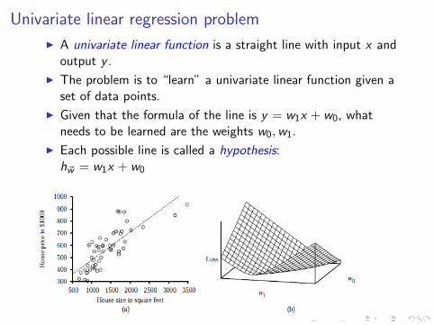
I A univariate linear function is a straight line with input x andoutput y .

I The problem is to “learn” a univariate linear function given aset of data points.

I Given that the formula of the line is y = w1x + w0, whatneeds to be learned are the weights w0,w1.

I Each possible line is called a hypothesis:h~w = w1x + w0

Univariate linear regression problem (cont’d)

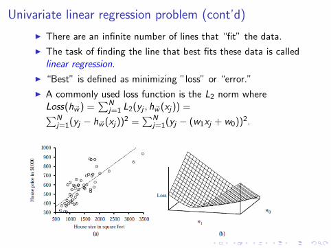
I There are an infinite number of lines that “fit” the data.

I The task of finding the line that best fits these data is calledlinear regression.

I “Best” is defined as minimizing ”loss” or “error.”

I A commonly used loss function is the L2 norm whereLoss(h~w ) =

∑Nj=1 L2(yj , h~w (xj)) =∑N

j=1(yj − h~w (xj))2 =∑N

j=1(yj − (w1xj + w0))2.

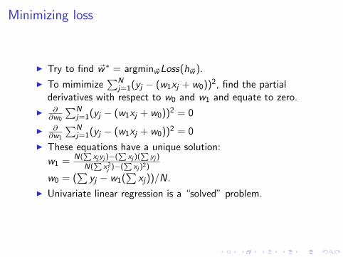
Minimizing loss

I Try to find ~w∗ = argmin~wLoss(h~w ).

I To mimimize∑N

j=1(yj − (w1xj + w0))2, find the partialderivatives with respect to w0 and w1 and equate to zero.

I ∂∂w0

∑Nj=1(yj − (w1xj + w0))2 = 0

I ∂∂w1

∑Nj=1(yj − (w1xj + w0))2 = 0

I These equations have a unique solution:

w1 =N(

Pxjyj )−(

Pxj )(

Pyj )

N(P

x2j )−(

Pxj )2)

w0 = (∑

yj − w1(∑

xj))/N.

I Univariate linear regression is a “solved” problem.

Beyond linear models

I The equations for minimum loss no longer have a closed-formsolution.

I Use a hill-climbing algorithm, gradient descent.

I The idea is to always move to a neighbor that is “better.”

I The algorithm is:~w ← any point in the parameter spaceloop until convergence dofor each wi in ~w dowi ← wi − α ∂

∂wiLoss(~w)

I α is called the step size or the learning rate.

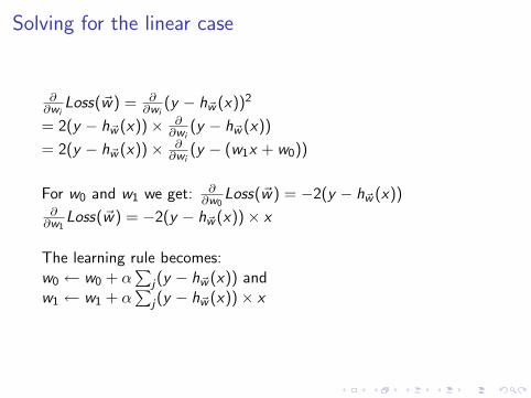
Solving for the linear case

∂∂wi

Loss(~w) = ∂∂wi

(y − h~w (x))2

= 2(y − h~w (x))× ∂∂wi

(y − h~w (x))

= 2(y − h~w (x))× ∂∂wi

(y − (w1x + w0))

For w0 and w1 we get: ∂∂w0

Loss(~w) = −2(y − h~w (x))∂

∂w1Loss(~w) = −2(y − h~w (x))× x

The learning rule becomes:w0 ← w0 + α

∑j(y − h~w (x)) and

w1 ← w1 + α∑

j(y − h~w (x))× x

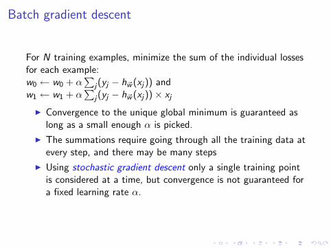
Batch gradient descent

For N training examples, minimize the sum of the individual lossesfor each example:w0 ← w0 + α

∑j(yj − h~w (xj)) and

w1 ← w1 + α∑

j(yj − h~w (xj))× xj

I Convergence to the unique global minimum is guaranteed aslong as a small enough α is picked.

I The summations require going through all the training data atevery step, and there may be many steps

I Using stochastic gradient descent only a single training pointis considered at a time, but convergence is not guaranteed fora fixed learning rate α.

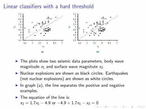
Linear classifiers with a hard threshold

I The plots show two seismic data parameters, body wavemagnitude x1 and surface wave magnitute x2.

I Nuclear explosions are shown as black circles. Earthquakes(not nuclear explosions) are shown as white circles.

I In graph (a), the line separates the positive and negativeexamples.

I The equation of the line is:x2 = 1.7x1 − 4.9 or −4.9 + 1.7x1 − x2 = 0

Classification hypothesis

I The classification hypothesis is:h~w = 1 if ~w .~x ≥ 0 and 0 otherwise

I It can be thought of passing the linear function ~w .~x through athreshold function.

I Mimimizing Loss depends on taking the gradient of thethreshold function

I The gradient for the step function is zero almost everywhereand undefined elsewhere!

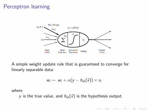
Perceptron learning

A simple weight update rule that is guaranteed to converge forlinearly separable data:

wi ← wi + α(y − h~w (~x))× xi

wherey is the true value, and h~w (~x) is the hypothesis output.

Perceptron learning rule

wi ← wi + α(y − h~w (~x))× xi

I If the output is correct, i.e., y = h~w (~x), then the weights arenot changed.

I If the output is lower than it should be, i.e, y is 1 but h~w (~x) is0, then wi is increased when the corresponding input xi ispositive and decreased when the corresponding input xi isnegative.

I If the output is higher than it should be, i.e, y is 0 but h~w (~x)is 1, then wi is decreased when the corresponding input xi ispositive and increased when the corresponding input xi isnegative.

Perceptron learning procedure

I Start with a random assignment to the weights

I Feed the input, let the perceptron compute the answer

I If the answer is correct, do nothing

I If the answer is not correct, update the weights by adding orsubtracting the input vector (scaled down by α)

I Iterate over all the input vectors, repeating as necessary, untilthe perceptron learns

Perceptron learning example

This example teaches the logical or function.a0 is the “bias”, a1 and a2 are the inputs, y is the output.

a0 a1 a2 y

Example 1 1 0 0 0

Example 2 1 0 1 1

Example 3 1 1 0 1

Example 4 1 1 1 1

With α = 0.5 and (0.1, 0.2, 0.3) as the initial weights, the weightvector converges to (−0.4, 0.7, 0.8) after 4 iterations on theexamples. The number of iterations changes depending on theinitial weights and α (see the spreadsheet).

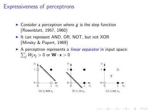
Expressiveness of perceptrons

I Consider a perceptron where g is the step function(Rosenblatt, 1957, 1960)

I It can represent AND, OR, NOT, but not XOR(Minsky & Papert, 1969)

I A perceptron represents a linear separator in input space:∑j Wjxj > 0 or W · x > 0

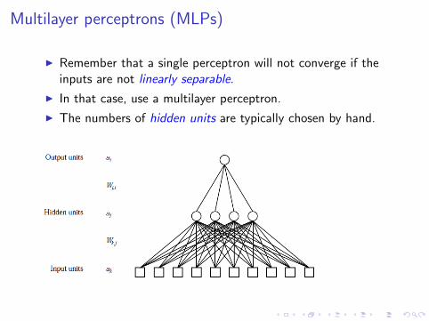
Multilayer perceptrons (MLPs)

I Remember that a single perceptron will not converge if theinputs are not linearly separable.

I In that case, use a multilayer perceptron.

I The numbers of hidden units are typically chosen by hand.

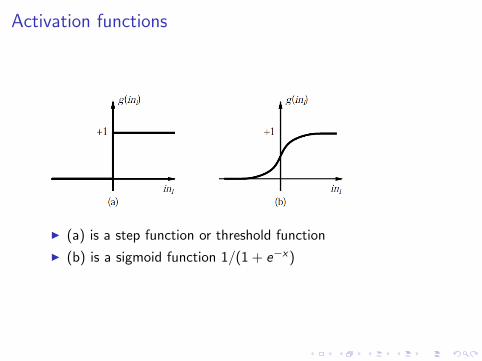
Activation functions

I (a) is a step function or threshold function

I (b) is a sigmoid function 1/(1 + e−x)

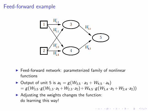
Feed-forward example

I Feed-forward network: parameterized family of nonlinearfunctions

I Output of unit 5 is a5 = g(W3,5 · a3 + W4,5 · a4)= g(W3,5 ·g(W1,3 ·a1+W2,3 ·a2)+W4,5 ·g(W1,4 ·a1+W2,4 ·a2))

I Adjusting the weights changes the function:do learning this way!

Single-layer perceptrons

I Output units all operate separately – no shared weights

I Adjusting the weights moves the location, orientation, andsteepness of cliff

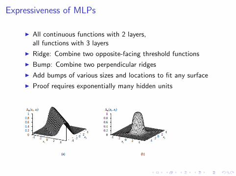
Expressiveness of MLPs

I All continuous functions with 2 layers,all functions with 3 layers

I Ridge: Combine two opposite-facing threshold functions

I Bump: Combine two perpendicular ridges

I Add bumps of various sizes and locations to fit any surface

I Proof requires exponentially many hidden units

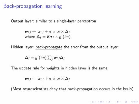
Back-propagation learning

Output layer: similar to a single-layer perceptron

wi ,j ← wi ,j + α× ai ×∆j

where ∆j = Err j × g ′(inj)

Hidden layer: back-propagate the error from the output layer:

∆i = g ′(ini )∑

j wi ,j∆j

The update rule for weights in hidden layer is the same:

wi ,j ← wi ,j + α× ai ×∆j

(Most neuroscientists deny that back-propagation occurs in the brain)

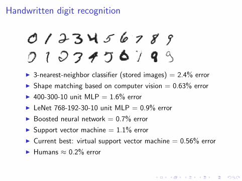
Handwritten digit recognition

I 3-nearest-neighbor classifier (stored images) = 2.4% error

I Shape matching based on computer vision = 0.63% error

I 400-300-10 unit MLP = 1.6% error

I LeNet 768-192-30-10 unit MLP = 0.9% error

I Boosted neural network = 0.7% error

I Support vector machine = 1.1% error

I Current best: virtual support vector machine = 0.56% error

I Humans ≈ 0.2% error

MLP learners

I MLPs are quite good for complex pattern recognition tasks

I The resulting hypotheses cannot be understood easily

I Typical problems: slow convergence, local minima

Understanding the brain

“The brain is a tissue. It is a complicated, intricately woven tissue,like nothing else we know of in the universe, but it is composed ofcells, as any tissue is. They are, to be sure, highly specialized cells,but they function according to the laws that govern any other cells.Their electrical and chemical signals can be detected, recorded andinterpreted and their chemicals can be identified, the connectionsthat constitute the brains woven feltwork can be mapped. In short,the brain can be studied, just as the kidney can.”

– David H. Hubel (1981 Nobel Prize Winner)

Understanding the brain (cont’d)

“Because we do not understand the brain very well we areconstantly tempted to use the latest technology as a model fortrying to understand it. In my childhood we were always assuredthat the brain was a telephone switchboard. (What else could itbe?) I was amused to see that Sherrington, the great Britishneuroscientist, thought that the brain worked like a telegraphsystem. Freud often compared the brain to hydraulic andelectro-magnetic systems. Leibniz compared it to a mill, and I amtold that some of the ancient Greeks thought the brain functionslike a catapult. At present, obviously, the metaphor is the digitalcomputer.”

– John R. Searle (Prof. of Philosophy at UC, Berkeley)

Summary

I Brains have lots of neurons; each neuron ≈ perceptron (?)

I None of the neural network models distinguish humans fromdogs from dolphins from flatworms. Whatever distinguisheshigher cognitive capacities (language, reasoning) may not beapparent at this level of analysis.

I Actually, real neurons fire all the time; what changes is therate of firing, from a few to a few hundred impulses a second.

I “Neurally inspired computing” rather than “brain science”.

I Perceptrons (one-layer networks) are used for linearlyseparable data.

I Multi-layer networks are sufficiently expressive; can be trainedby gradient descent, i.e., error back-propagation.

I Many applications: speech, driving, handwriting, frauddetection, etc.

I Engineering, cognitive modelling, and neural system modellingsubfields have largely diverged

Sources for the slides

I AIMA textbook (3rd edition)

I AIMA slides:http://aima.cs.berkeley.edu/

I Neuron cell:http://www.enchantedlearning.com/subjects/anatomy/brain/Neuron.shtml

(Accessed December 10, 2011)

I Robert Wilensky’s CS188 slideshttp://www.cs.berkeley.edu/ wilensky/cs188

(Accessed prior to 2009)