EPA/452/B-02-001

Section 5

SO2 and Acid Gas Controls

EPA/452/B-02-001

Section 5.2

Post-Combustion Controls

EPA/452/B-02-001

Chapter 1

WET SCRUBBERS FOR ACID GAS

Wiley Barbour Roy Oommen Gunseli Sagun Shareef Radian Corporation Research Triangle Park, NC 27709

William M. Vatavuk Innovative Strategies and Economics Group, OAQPS U.S. Environmental Protection Agency Research Triangle Park, NC 27711

December 1995

Contents

1.0 Introduction ............................................................................................................................................ 1-3 1.1 System Efficiencies and Performance ..................................................................................................... 1-3

1.2 Process Description ................................................................................................................................ 1-4 1.2.1 Absorber System Configuration ................................................................................................... 1-4 1.2.2 Types of Absorption Equipment ................................................................................................... 1-5 1.2.3 Packed Tower Interals ................................................................................................................... 1-6 1.2.4 Packed Tower Operation ............................................................................................................... 1-9

1.3 Design Procedures ............................................................................................................................... 1-10 1.3.1 Determining Gas and Liquid Stream Conditions ......................................................................... 1-11 1.3.2 Determining Absorption Factor .................................................................................................. 1-15 1.3.3 Determining Column Diameter .................................................................................................... 1-16 1.3.4 Determining Tower Height and Surface Area ............................................................................. 1-18 1.3.5 Calculating Column Pressure Drop ............................................................................................. 1-20 1.3.6 Alternative Design Procedure .................................................................................................... 1-21

1.4 Estimating Total Capital Investment ..................................................................................................... 1-23 1.4.1 Equipment Costs for Packed Towers .......................................................................................... 1-23 1.4.2 Installation Costs ........................................................................................................................ 1-25

1.5 Estimating Annual Cost ........................................................................................................................ 1-26 1.5.1 Direct Annual Costs ................................................................................................................... 1-26 1.5.2 Indirect Annual Costs ................................................................................................................ 1-28 1.5.3 Total Annual Costs ..................................................................................................................... 1-30

1.6 Example Problem ................................................................................................................................... 1-30 1.6.1 Required Information for Design ................................................................................................ 1-30 1.6.2 Determine Gas and Liquid Stream Properties .............................................................................. 1-31 1.6.3 Calculate Absorption Factor ....................................................................................................... 1-34 1.6.4 Estimate Column Diameter ......................................................................................................... 1-34 1.6.5 Calculate Column Surface Area .................................................................................................. 1-36 1.6.6 Calculate Pressure Drop ............................................................................................................. 1-37 1.6.7 Equipment Costs ......................................................................................................................... 1-37 1.6.8 Total Annual Cost ...................................................................................................................... 1-39 1.6.9 Alternate Example ....................................................................................................................... 1-43

1.7 Acknowledgements .............................................................................................................................. 1-43

References .................................................................................................................................................. 1-44

Appendix A ................................................................................................................................................. 1-46 Appendix B ................................................................................................................................................. 1-50 Appendix C ................................................................................................................................................. 1-54

1-2

1.0 Introduction

Gas absorbers are used extensively in industry for separation and purification of gas streams, as product recovery devices, and as pollution control devices. This chapter focuses on the application of absorption for pollution control on gas streams with typical pollutant concentrations ranging from 250 to 10,000 ppmv. Gas absorbers are most widely used to remove water soluble inorganic contaminants from air streams.[l, 2]

Absorption is a process where one or more soluble components of a gas mixture are dissolved in a liquid (i.e., a solvent). The absorption process can be categorized as physical or chemical. Physical absorption occurs when the absorbed compound dissolves in the solvent; chemical absorption occurs when the absorbed compound and the solvent react. Liquids commonly used as solvents include water, mineral oils, nonvolatile hydrocarbon oils, and aqueous solutions.[1]

1.1 System Efficiencies and Performance

Removal efficiencies for gas absorbers vary for each pollutant-solvent system and with the type of absorber used. Most absorbers have removal efficiencies in excess of 90 percent, and packed tower absorbers may achieve efficiencies as high as 99.9 percent for some pollutant-solvent systems.[1, 3]

The suitability of gas absorption as a pollution control method is generally dependent on the following factors: 1) availability of suitable solvent; 2) required removal efficiency; 3) pollutant concentration in the inlet vapor; 4) capacity required for handling waste gas; and, 5) recovery value of the pollutant(s) or the disposal cost of the spent solvent.[4]

Physical absorption depends on properties of the gas stream and solvent, such as density and viscosity, as well as specific characteristics of the pollutant(s) in the gas and the liquid stream (e.g., diffusivity, equilibrium solubility). These properties are temperature dependent, and lower temperatures generally favor absorption of gases by the solvent.[1] Absorption is also enhanced by greater contacting surface, higher liquid-gas ratios, and higher concentrations in the gas stream.[1]

The solvent chosen to remove the pollutant(s) should have a high solubility for the gas, low vapor pressure, low viscosity, and should be relatively inexpensive.[4] Water is the most common solvent used to remove inorganic contaminants; it is also used to absorb organic compounds having relatively high water solubilities. For organic compounds that have low water solubilities, other solvents such as hydrocarbon oils are used, though only in industries where large volumes of these oils are available (i.e., petroleum refineries and petrochemical plants).[5]

1-3

Pollutant removal may also be enhanced by manipulating the chemistry of the absorbing solution so that it reacts with the pollutant(s), e.g., caustic solution for acid-gas absorption vs. pure water as a solvent. Chemical absorption may be limited by the rate of reaction, although the rate limiting step is typically the physical absorption rate, not the chemical reaction rate.

1.2 Process Description

Absorption is a mass transfer operation in which one or more soluble components of a gas mixture are dissolved in a liquid that has low volatility under the process conditions. The pollutant diffuses from the gas into the liquid when the liquid contains less than the equilibrium concentration of the gaseous component. The difference between the actual concentration and the equilibrium concentration provides the driving force for absorption.

A properly designed gas absorber will provide thorough contact between the gas and the solvent in order to facilitate diffusion of the pollutant(s). It will perform much better than a poorly designed absorber.[6] The rate of mass transfer between the two phases is largely dependent on the surface area exposed and the time of contact. Other factors governing the absorption rate, such as the solubility of the gas in the particular solvent and the degree of the chemical reaction, are characteristic of the constituents involved and are relatively independent of the equipment used.

1.2.1 Absorber System Configuration

Gas and liquid flow through an absorber may be countercurrent, crosscurrent, or cocurrent. The most commonly installed designs are countercurrent, in which the waste gas stream enters at the bottom of the absorber column and exits at the top. Conversely, the solvent stream enters at the top and exits at the bottom. Countercurrent designs provide the highest theoretical removal efficiency because gas with the lowest pollutant concentration contacts liquid with the lowest pollutant concentration. This serves to maximize the average driving force for absorption throughout the column.[2] Moreover, countercurrent designs usually require lower liquid to gas ratios than cocurrent and are more suitable when the pollutant loading is higher.[3, 5]

In a crosscurrent tower, the waste gas flows horizontally across the column while the solvent flows vertically down the column. As a rule, crosscurrent designs have lower pressure drops and require lower liquid-to-gas ratios than both cocurrent and countercurrent designs. They are applicable when gases are highly soluble, since they offer less contact time for absorption.[2, 5]

In cocurrent towers, both the waste gas and solvent enter the column at the top of the tower and exit at the bottom. Cocurrent designs have lower pressure drops, are not subject to flooding limitations and are more efficient for fine (i.e., submicron) mist removal. Cocurrent designs are only efficient where large absorption driving forces are available. Removal efficiency is limited since the gas-liquid system approaches equilibrium at the bottom of the tower.[2]

1-4

1.2.2 Types of Absorption Equipment

Devices that are based on absorption principles include packed towers, plate (or tray) columns, venturi scrubbers, and spray chambers. This chapter focuses on packed towers, which are the most commonly used gas absorbers for pollution control. Packed towers are columns filled with packing materials that provide a large surface area to facilitate contact between the liquid and gas. Packed tower absorbers can achieve higher removal efficiencies, handle higher liquid rates, and have relatively lower water consumption requirements than other types of gas absorbers.[2] However, packed towers may also have high system pressure drops, high clogging and fouling potential, and extensive maintenance costs due to the presence of packing materials. Installation, operation, and wastewater disposal costs may also be higher for packed bed absorbers than for other absorbers.[2] In addition to pump and fan power requirements and solvent costs, packed towers have operating costs associated with replacing damaged packing.[2]

Plate, or tray, towers are vertical cylinders in which the liquid and gas are contacted in step-wise fashion on trays (plates). Liquid enters at the top of the column and flows across each plate and through a downspout (downcomer) to the plates below. Gas moves upwards through openings in the plates, bubbles into the liquid, and passes to the plate above. Plate towers are easier to clean and tend to handle large temperature fluctuations better than packed towers do.[4] However, at high gas flow rates, plate towers exhibit larger pressure drops and have larger liquid holdups. Plate towers are generally made of materials such as stainless steel, that can withstand the force of the liquid on the plates and also provide corrosion protection. Packed columns are preferred to plate towers when acids and other corrosive materials are involved because tower construction can then be of fiberglass, polyvinylchloride, or other less costly, corrosive-resistant materials. Packed towers are also preferred for columns smaller than two feet in diameter and when pressure drop is an important consideration.[3, 7]

Venturi scrubbers are generally applied for controlling particulate matter and sulfur dioxide. They are designed for applications requiring high removal efficiencies of submicron particles, between 0.5 and 5.0 micrometers in diameter.[4] A venturi scrubber employs a gradually converging and then diverging section, called the throat, to clean incoming gaseous streams. Liquid is either introduced to the venturi upstream of the throat or injected directly into the throat where it is atomized by the gaseous stream. Once the liquid is atomized, it collects particles from the gas and discharges from the venturi.[1] The high pressure drop through these systems results in high energy use, and the relatively short gas-liquid contact time restricts their application to highly soluble gases. Therefore, they are infrequently used for the control of volatile organic compound emissions in dilute concentration.[2]

Spray towers operate by delivering liquid droplets through a spray distribution system. The droplets fall through a countercurrent gas stream under the influence of gravity and contact the pollutant(s) in the gas.[7] Spray towers are simple to operate and maintain, and have relatively low

1-5

Figure 1.1: Packed Tower for Gas Absorption

energy requirements. However, they have the least effective mass transfer capability of the absorbers discussed and are usually restricted to particulate removal and control of highly soluble gases such as sulfur dioxide and ammonia. They also require higher water recirculation rates and are inefficient at removing very small particles.[2, 5]

1.2.3 Packed Tower Internals

A basic packed tower unit is comprised of a column shell, mist eliminator, liquid distributors, packing materials, packing support, and may include a packing restrainer. Corrosion resistant alloys or plastic materials such as polypropylene are required for column internals when highly corrosive solvents or gases are used. A schematic drawing of a countercurrent packed tower is shown in Figure 1.1. In this figure, the packing is separated into two sections. This configuration is more expensive than designs where the packing is not so divided.[5]

1-6

The tower shell may be made of steel or plastic, or a combination of these materials depending on the corrosiveness of the gas and liquid streams, and the process operating conditions. One alloy that is chemical and temperature resistant or multiple layers of different, less expensive materials may be used. The shell is sometimes lined with a protective membrane, often made from a corrosion resistant polymer. For absorption involving acid gases, an interior layer of acid resistant brick provides additional chemical and temperature resistance.[8]

At high gas velocities, the gas exiting the top of the column may carry off droplets of liquid as a mist. To prevent this, a mist eliminator in the form of corrugated sheets or a layer of mesh can be installed at the top of the column to collect the liquid droplets, which coalesce and fall back into the column.

A liquid distributor is designed to wet the packing bed evenly and initiate uniform contact between the liquid and vapor. The liquid distributor must spread the liquid uniformly, resist plugging and fouling, provide free space for gas flow, and allow operating flexibility.[9] Large towers frequently have a liquid redistributor to collect liquid off the column wall and direct it toward the center of the column for redistribution and enhanced contact in the lower section of packing.[4] Liquid redistributors are generally required for every 8 to 20 feet of random packing depth.[5, 10]

Distributors fall into two categories: gravitational types, such as orifice and weir types, and pressure-drop types, such as spray nozzles and perforated pipes. Spray nozzles are the most common distributors, but they may produce a fine mist that is easily entrained in the gas flow. They also may plug, and usually require high feed rates to compensate for poor distribution. Orifice-type distributors typically consist of flat trays with a number of risers for vapor flow and perforations in the tray floor for liquid flow. The trays themselves may present a resistance to gas flow.[9] However, better contact is generally achieved when orifice distributors are used.[3]

Packing materials provide a large wetted surface for the gas stream maximizing the area available for mass transfer. Packing materials are available in a variety of forms, each having specific characteristics with respect to surface area, pressure drop, weight, corrosion resistance, and cost. Packing life varies depending on the application. In ideal circumstances, packing will last as long as the tower itself. In adverse environments packing life may be as short as 1 to 5 years due to corrosion, fouling, and breakage.[11]

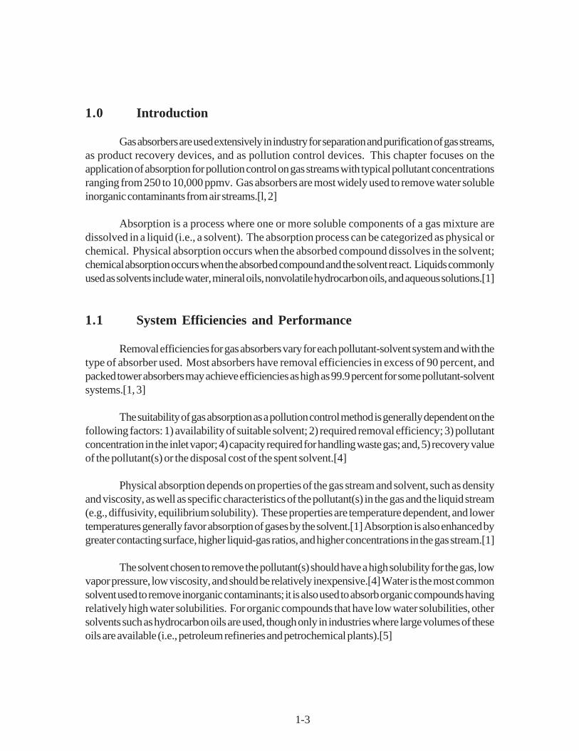
Packing materials are categorized as random or structured. Random packings are usually dumped into an absorption column and allowed to settle. Modern random packings consist of engineered shapes intended to maximize surface-to-volume ratio and minimize pressure drop.[2] Examples of different random packings are presented in Figure 1.2. The first random packings specifically designed for absorption towers were made of ceramic. The use of ceramic has declined because of their brittleness, and the current markets are dominated by metal and plastic. Metal packings cannot be used for highly corrosive pollutants, such as acid gas, and plastic packings are not suitable for high temperature applications. Both plastic and metal packings are generally limited to an unsupported depth of 20 to 25. At higher depths the weight may deform the packing.[10]

1-7

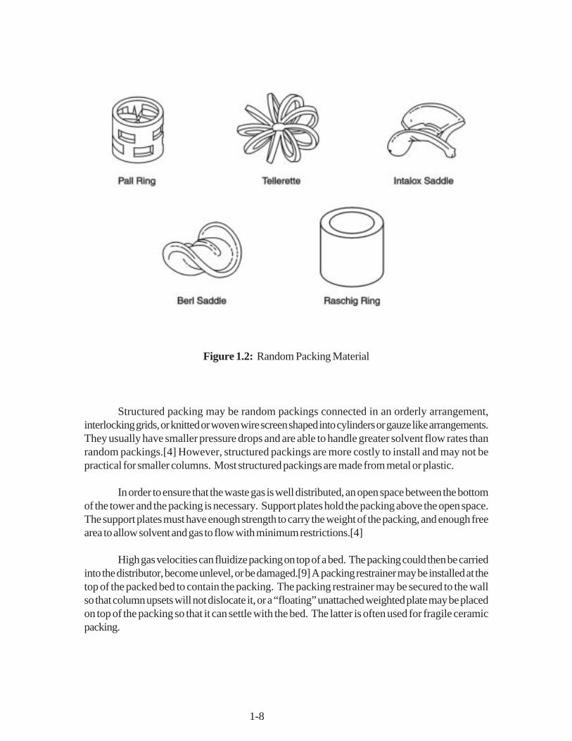
Figure 1.2: Random Packing Material

Structured packing may be random packings connected in an orderly arrangement, interlocking grids, or knitted or woven wire screen shaped into cylinders or gauze like arrangements. They usually have smaller pressure drops and are able to handle greater solvent flow rates than random packings.[4] However, structured packings are more costly to install and may not be practical for smaller columns. Most structured packings are made from metal or plastic.

In order to ensure that the waste gas is well distributed, an open space between the bottom of the tower and the packing is necessary. Support plates hold the packing above the open space. The support plates must have enough strength to carry the weight of the packing, and enough free area to allow solvent and gas to flow with minimum restrictions.[4]

High gas velocities can fluidize packing on top of a bed. The packing could then be carried into the distributor, become unlevel, or be damaged.[9] A packing restrainer may be installed at the top of the packed bed to contain the packing. The packing restrainer may be secured to the wall so that column upsets will not dislocate it, or a “floating” unattached weighted plate may be placed on top of the packing so that it can settle with the bed. The latter is often used for fragile ceramic packing.

1-8

1.2.4 Packed Tower Operation

As discussed in Section 1.2.1, the most common packed tower designs are countercurrent. As the waste gas flows up the packed column it will experience a drop in its pressure as it meets resistance from the packing materials and the solvent flowing down. Pressure drop in a column is a function of the gas and liquid flow rates and properties of the packing elements, such as surface area and free volume in the tower. A high pressure drop results in high fan power to drive the gas through the packed tower. and consequently high costs. The pressure drop in a packed tower generally ranges from 0.5 to 1.0 in. H

2O/ft of packing.[7]

For each column, there are upper and lower limits to solvent and vapor flow rates that ensure satisfactory performance. The gas flow rate may become so high that the drag on the solvent is sufficient to keep the solvent from flowing freely down the column. Solvent begins toaccumulate and blocks the entire cross section for flow, which increases the pressure drop and present the packing from mixing the gas and solvent effectively. When all the free volume in the packing is filled with liquid and the liquid is carried back up the column, the absorber is considered to be flooded.[4] Most packed towers operate at 60 to 70 percent of the gas flooding velocity, as it is not practical to operate a tower in a flooded condition.[7] A minimum liquid flow rate is also required to wet the packing material sufficiently for effective mass transfer to occur between the gas and liquid.[7]

The waste gas inlet temperature is another important scrubbing parameter. In general, the higher the gas temperature, the lower the absorption rate, and vice-versa. Excessively high gas temperatures also can lead to significant solvent loss through evaporation. Consequently, precoolers (e.g., spray chambers) may be needed to reduce the air temperature to acceptable levels.[6]

For operations that are based on chemical reaction with absorption, an additional concern is the rate of reaction between the solvent and pollutant(s). Most gas absorption chemical reactions are relatively fast and the rate limiting step is the physical absorption of the pollutants into the solvent. However, for solvent-pollutant systems where the chemical reaction is the limiting step, the rates of reaction would need to be analyzed kinetically.

Heat may be generated as a result of exothermal chemical reactions. Heat may also be generated when large amounts of solute are absorbed into the liquid phase, due to the heat of solution. The resulting change in temperature along the height of the absorber column may damage equipment and reduce absorption efficiency. This problem can be avoided by adding cooling coils to the column.[7] However, in those systems where water is the solvent, adiabatic saturation of the gas occurs during absorption due to solvent evaporation. This causes a substantial cooling of the absorber that offsets the heat generated by chemical reactions. Thus, cooling coils are rarely required with those systems.[5] In any event, packed towers may be designed assuming that isothermal conditions exist throughout the column.[7]

1-9

The effluent from the column may be recycled into the system and used again. This is usually the case if the solvent is costly, i.e., hydrocarbon oils, caustic solution. Initially, the recycle stream may go to a waste treatment system to remove the pollutants or the reaction product. Make-up solvent may then be added before the liquid stream reenters the column. Recirculation of the solvent requires a pump, solvent recovery system, solvent holding and mixing tanks, and any associated piping and instrumentation.

1.3 Design Procedures

The design of packed tower absorbers for controlling gas streams containing a mixture of pollutants and air depends on knowledge of the following parameters:

� Waste gas flow rate;

� Waste gas composition and concentration of the pollutants in the gas stream;

� Required removal efficiency;

� Equilibrium relationship between the pollutants and solvent; and

� Properties of the pollutant(s), waste gas, and solvent: diffusivity, viscosity, density, and molecular weight.

The primary objectives of the design procedures are to determine column surface area and pressure drop through the column. In order to determine these parameters, the following steps must be performed:

� Determine the gas and liquid stream conditions entering and exiting the column.

� Determine the absorption factor (AF).

� Determine the diameter of the column (D).

� Determine the tower height (H ) and surface area (S).tower

� Determine the packed column pressure drop ( P).

To simplify the sizing procedures, a number of assumptions have been made. For example, the waste gas is assumed to comprise a two-component waste gas mixture (pollutant/air), where the pollutant consists of a single compound present in dilute quantities. The waste gas is assumed to behave as an ideal gas and the solvent is assumed to behave as an ideal solution. Heat effects associated with absorption are considered to be minimal for the pollutant concentrations

1-10

encountered. The procedures also assume that, in chemical absorption, the process is not reaction rate limited, i.e., the reaction of the pollutant with the solvent is considered fast compared to the rate of absorption of the pollutant into the solvent.

The design procedures presented here are complicated, and careful attention to units is required. Appendix A has a list of all design variables referred to in this chapter, along with the appropriate units.

1.3.1 Determining Gas and Liquid Stream Conditions

Gas absorbers are designed based on the ratio of liquid to gas entering the column (Li/G

i),

slope of the equilibrium curve (m), and the desired removal efficiency (η). These factors are calculated from the inlet and outlet gas and liquid stream variables:

� Waste gas flow rate, in actual cubic feet per minute (acfm), entering and exiting column (G

i and G

o, respectively);

� Pollutant concentration (lb-moles pollutant per lb-mole of pollutant free gas) enter-ing and exiting the column in the waste gas (Y

i and Y

o, respectively);

� Solvent flow rate, in gallons per minute (gpm), entering and exiting the column (Li

and Lo, respectively); and

� Pollutant concentration (lb-moles pollutant per lb-mole of pollutant free solvent) entering and exiting the column in the solvent (X

i and X

o, respectively).

This design approach assumes that the inlet gas stream variables are known, and that a specific pollutant removal efficiency has been chosen as the design basis; i.e., the variables G

i, Y

i,

andη are known. For dilute concentrations typically encountered in pollution control applications and negligible changes in moisture content, G

i is assumed equal to G

o. If a once-through process

is used, or if the spent solvent is regenerated by an air stripping process before it is recycled, the value of X

i will approach zero. The following procedures must be followed to calculate the remaining

stream variablesYo, L

i (andL

o), and X

o . A schematic diagram of a packed tower with inlet and outlet

flow and concentration variables labeled is presented in Figure 1.3.

The exit pollution concentration, Yo, may be calculated from using the following equation:

η Y = Y 1 -o i (1.1) 10 0

1-11

Figure 1.3: Schematic Diagram of Countercurrent Packed Bed Operation

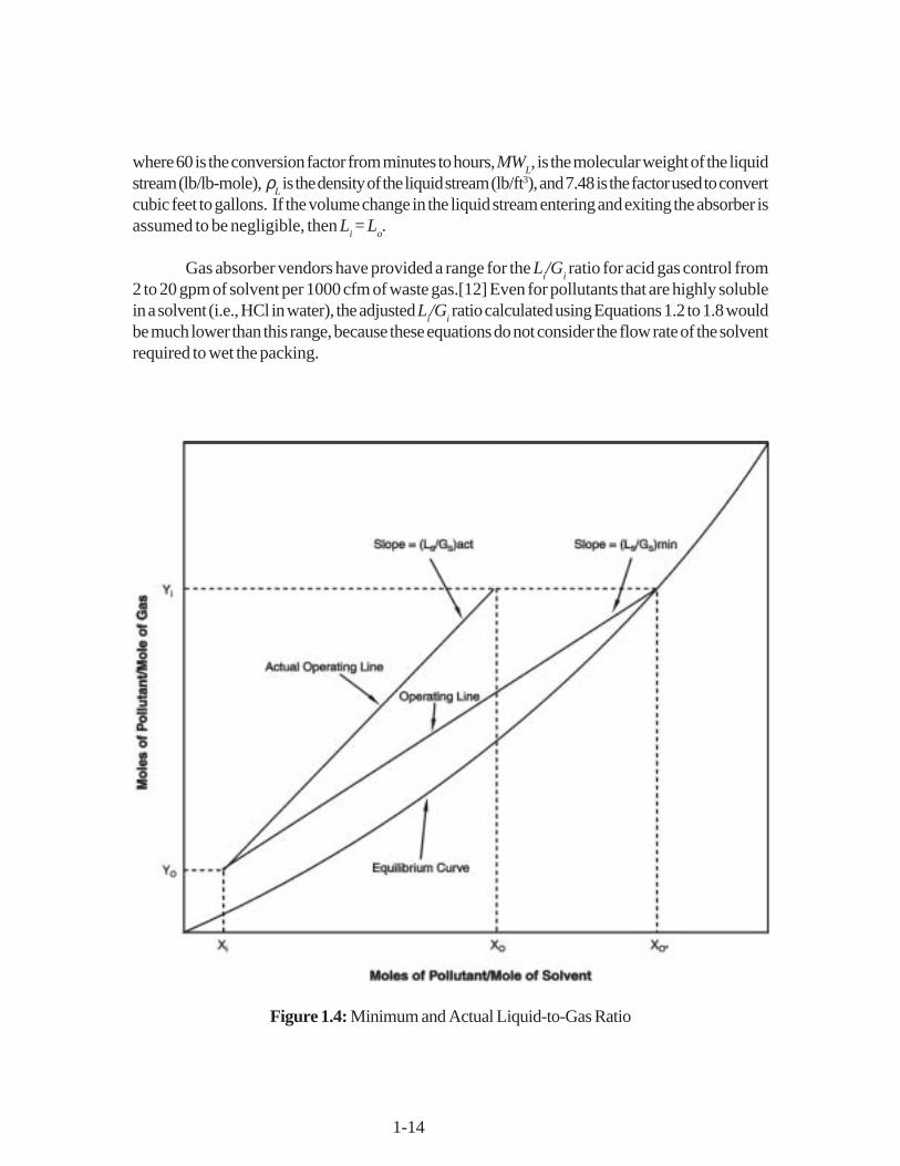
The liquid flow rate entering the absorber, Li (gpm), is then calculated using a graphical

method. Figure 1.4 presents an example of an equilibrium curve and operating line. The equilibrium curve indicates the relationship between the concentration of pollutant in the waste gas and the concentration of pollutant in the solvent at a specified temperature. The operating line indicates the relation between the concentration of the pollutant in the gas and solvent at any location in the gas absorber column. The vertical distance between the operating line and equilibrium curve indicates the driving force for diffusion of the pollutant between the gas and liquid phases. The minimum amount of liquid which can be used to absorb the pollutant in the gas stream corresponds to an operating line drawn from the outlet concentration in the gas stream (Y

o) and the inlet concentration

in the solvent stream (Xi) to the point on the equilibrium curve corresponding to the entering pollutant

concentration in the gas stream (Yi). At the intersection point on the equilibrium curve, the diffusional

driving forces are zero, the required time of contact for the concentration change is infinite, and an infinitely tall tower results.

The slope of the operating line intersecting the equilibrium curve is equal to the minimumL/ G ratio on a moles of pollutant-free solvent (L

s) per moles of pollutant-free gas basis G

s . in other

words, the values Ls and G

s do not include the moles of pollutant in the liquid and gas streams. The

values of Ls and G

s are constant through the column if a negligible amount of moisture is transferred

1-12

from the liquid to the gas phase. The slope may be calculated from the following equation:

L Y - Yis

s

o (1.2)

= *G X - X im in o

whereX*o would be the maximum concentration of the pollutant in the liquid phase if it were allowed

to come to equilibrium with the pollutant entering the column in the gas phase, Yi. The value of X*

o

is taken from the equilibrium curve. Because the minimumLs/G

s, ratio is an unrealistic value, it must

be multiplied by an adjustment factor, commonly between 1.2 and 1.5, to calculate the actual L/G ratio:[7]

L Ls

s

s

s

=

× (ad jus tm en t fac to r) (1.3)G G m in ac t

The variable Gs may be calculated using the equation:

6 0 ρ GG iG (1.4)= s M W G (1 + Yi )

where 60 is the conversion factor from minutes to hours, MWG, is the molecular weight of the gas

stream (lb/lb-mole), andρG

is the density of the gas stream (lb/ft3). For pollutant concentrations typically encountered, the molecular weight and density of the waste gas stream are assumed to be equal to that of ambient air.

The variable Ls may then be calculated by:

L s

G s

L × G s (1.5)= s

ac t

The total molar flow rates of the gas and liquid entering the absorber (G and L ) aremol,i mol,i

calculated using the following equations:

G m ol, i = G s (1 + Yi ) (1.6)

L m ol, i = L s (1 + X i ) (1.7)

The volume flow rate of the solvent, Li, may then be calculated by using the following

relationship:

7 .48 L M W m ol,i LL =i (1.8)60 rL

1-13

where 60 is the conversion factor from minutes to hours,MWL, is the molecular weight of the liquid

stream (lb/lb-mole), ρL is the density of the liquid stream (lb/ft3), and 7.48 is the factor used to convert

cubic feet to gallons. If the volume change in the liquid stream entering and exiting the absorber is assumed to be negligible, then L

i = L

o.

Gas absorber vendors have provided a range for the Li/G

i ratio for acid gas control from

2 to 20 gpm of solvent per 1000 cfm of waste gas.[12] Even for pollutants that are highly soluble in a solvent (i.e., HCl in water), the adjusted L

i/G

i ratio calculated using Equations 1.2 to 1.8 would

be much lower than this range, because these equations do not consider the flow rate of the solvent required to wet the packing.

Figure 1.4: Minimum and Actual Liquid-to-Gas Ratio

1-14

Finally, the actual operating line may be represented by a material balance equation over the gas absorber:[4]

X L + Y Gi s i s = X L + Y Go s o s (1.9)

Equation 1.9 may then be solved for X : o

Yi - YoX + X= i o L (1.10)

s

G s

1.3.2 Determining Absorption Factor

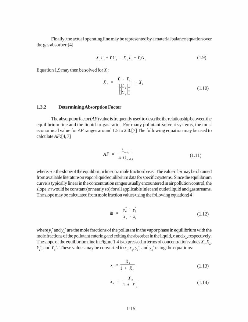
The absorption factor (AF) value is frequently used to describe the relationship between the equilibrium line and the liquid-to-gas ratio. For many pollutant-solvent systems, the most economical value for AF ranges around 1.5 to 2.0.[7] The following equation may be used to calculate AF:[4, 7]

Lm ol, i A F = (1.11)m G m ol, i

wherem is the slope of the equilibrium line on a mole fraction basis. The value ofmmay be obtained from available literature on vapor/liquid equilibrium data for specific systems. Since the equilibrium curve is typically linear in the concentration ranges usually encountered in air pollution control, the slope, mwould be constant (or nearly so) for all applicable inlet and outlet liquid and gas streams. The slope may be calculated from mole fraction values using the following equation:[4]

* * y - y m = o i

(1.12)x - xo i

where yi* and y

o* are the mole fractions of the pollutant in the vapor phase in equilibrium with the

mole fractions of the pollutant entering and exiting the absorber in the liquid, xiand x

o, respectively.

The slope of the equilibrium line in Figure 1.4 is expressed in terms of concentration values Xi, X

o,

Y *, and Y * . These values may be converted to x , x , y *, and y * using the equations:i o i o i o

X i x = (1.13)i 1 + X i

X o x =o (1.14)1 + X o

1-15

* Y* i y = i * (1.15)1 + Yi

*Y* oy =o * (1.16)1 + Yo

where the units for each of these variables are listed in Appendix A.

The absorption factor will be used to calculate the theoretical number of transfer units and the theoretical height of a transfer unit. First, however, the column diameter needs to be determined.

1.3.3 Determining Column Diameter

Once stream conditions have been determined, the diameter of the column may be estimated. The design presented in this section is based on selecting a fraction of the gas flow rate at flooding conditions. Alternatively, the column may be designed for a specific pressure drop (see Section 1.3.6.). Eckert’s modification to the generalized correlation for randomly packed towers based on flooding considerations is used to obtain the superficial gas flow rate entering the absorber, G (lb/sec-ft2), or the gas flow rate per crossectional area based on the L /G ratio calculated

sfr,i mol,i mol,i

in Section 1.3.2.[10] The cross-sectional area (A) of the column and the column diameter (D) can then be determined from G . Figure 1.5 presents the relationship between G and the L /

sfr,i sfr,i mol,i

G ratio at the tower flood point. The Abscissa value (X axis) in the graph is expressed as:[10]mol,i

L m ol, i M W L ρGA bscissa = (1.17) G m ol, i M W G ρL

The Ordinate value (Y axis) in the graph is expressed as:[10]

0 .2 2 µL ( )G Ψ F sfr, i p 2.42 (1.18)O rd ina te = ρ ρ gL G c

where Fp is a packing factor, g

c is the gravitational constant (32.2), µ

L is the viscosity of the solvent

(lb/ft-hr), 2.42 is the factor used to convert lb/ft-hr to centipoise, and Ψ is the ratio of the density of the scrubbing liquid to water. The value of F

p may be obtained from packing vendors (see

Appendix B, Table 1.8).

1-16

Figure 1.5: Eckert’s Modification to the Generalized Correlation at Flooding Rate

After calculating theAbscissavalue, a correspondingOrdinatevalue may determined from the floo ding curve. The Ordinate may also be calculated using the following equation:[10]

2[ −1.668 - 1.085 (lo g A b scissa ) -0 .297 (lo g A b scissa ) ] (1.19)O rd inate = 10

Equation 1.18 may then be rearranged to solve for G :sfr,i

ρ ρ g ( O rd ina te )1 G cG = sfr, i 0 .2 µ L (1.20)Fp Ψ 2.42

The cross-sectional area of the tower (ft2) is calculated as:

G M W m ol, i GA = (1.21)3,600 G fsfr,i

where f is the flooding factor and 3600 is the conversion factor from hours to seconds. To prevent flooding, the column is operated at a fraction of G . The value of f typically ranges from 0.60 to

sfr,i

1-17

0.75.[7]

The diameter of the column (ft) can be calculated from the cross-sectional area, by:

4D = A (1.22)

π

If a substantial change occurs between inlet and outlet volumes (i.e., moisture is transferred from the liquid phase to the gas phase), the diameter of the column will need to be calculated at the top and bottom of the column. The larger of the two values is then chosen as a conservative number. As a rule of thumb, the diameter of the column should be at least 15 times the size of the packing used in the column. If this is not the case, the column diameter should be recalculated using a smaller diameter packing.[10]

The superficial liquid flow rate entering the absorber, L (lb/hr-ft2 based on the cross-sfr,i

sectional area determined in Equation 1.21 is calculated from the equation:

L M Wm ol, i LL sfr, i = (1.23)A

For the absorber to operate properly, the liquid flow rate entering the column must be high enough to effectively wet the packing so mass transfer between the gas and liquid can occur. The minimum value of L that is required to wet the packing effectively can be calculated using the

sfr,i

equation:[7, 13]

(L )m in

= M W R ρ a (1.24)s fr, i L

where MWR is defined as the minimum wetting rate (ft2/hr), anda is the surface area to volume ratio of the packing (ft2/ft3). AnMWR value of 0.85 ft2/hr is recommended for ring packings larger than 3 inches and for structured grid packings. For other packings, an MWR of 1.3 ft2/hr is recommended.[7,13] Appendix B, Table 1.8 contains values of a for common packing materials.

If L (the value calculated in Equation 1.23) is smaller than (L ) (the value calculatedsfr,i sfr, min

in Equation 1.24), there is insufficient liquid flow to wet the packing using the current design parameters. The value of G , and A then will need to be recalculated. See Appendix C for details.

sfr,i

1.3.4 Determining Tower Height and Surface Area

Tower height is primarily a function of packing depth. The required depth of packing (Hpack

) is determined from the theoretical number of overall transfer units (N

tu) needed to achieve a specific

removal efficiency, and the height of the overall transfer unit (Htu):[4]

1-18

H pack = N tu H tu (1.25)

The number of overall transfer units may be estimated graphically by stepping off stages on the equilibrium-operating line graph from inlet conditions to outlet conditions, or by the following equation:[4]

1

1y - m xi i

y - m xo i

ln 1 -

+ A F A F

N = tu (1.26)11 -

A F

where ln is the natural logarithm of the quantity indicated.

The equation is based on several assumptions: 1) Henry’s law applies for a dilute gas mixture; 2) the equilibrium curve is linear from x

i to x

o; and 3) the pollutant concentration in the

solvent is dilute enough such that the operating line can be considered a straight line.[4]

If xi≈ 0 (i.e., a negligible amount of pollutant enters the absorber in the liquid stream) and

1/A≈ 0 (i.e., the slope of the equilibrium line is very small and/or the L /G ratio is very large),mol mol

Equation 1.26 simplifies to:

y i

y o

N = ln (1.27)tu

There are several methods that may be used to calculate the height of the overall transfer unit, all based on empirically determined packing constants. One commonly used method involves determining the overall gas and liquid mass transfer coefficients (K

G, K

L). A major difficulty in using

this approach is that values forKG andK

L are frequently unavailable for the specific pollutant-solvent

systems of interest. The reader is referred to the book Random Packing and Packed Tower Design Applications in the reference section for further details regarding this method.[14]

For this chapter, the method used to calculate the height of the overall transfer unit is based on estimating the height of the gas and liquid film transfer units, H

L and H

G, respectively:[4]

1H = H + Htu G L (1.28)

A F

The following correlations may be used to estimate values for HL and H

G:[13]

3,6 0 0 f G sfr, i

(L sfr, i )Γ

)β

ρ (

α

µGH = (1.29)G DG G

1-19

b L sfr, i µH L = φ L (1.30)

µ ρ DL L L

The quantity µ / ρ D is the Schmidt number and the variables β , b and Γ are packing constants specific to each packing type. Typical values for these constants are listed in Appendix B, Tables 1.9 and 1.10. The advantage to using this estimation method is that the packing constants may be applied to any pollutant-solvent system. One packing vendor offers the following modifications to Equations 1.29 and 1.30 for their specific packing:[15]

β 3,6 0 0 f G Γ ( s fr, i ) µG µ L H G = α Γ β (1.31)

(L ) ρG D G µG s fr, i

b −4 .255 L sfr, i µ L T H L = φ (1.32)

µ L ρL D L 2 86

where T is the temperature of the solvent in Kelvin.

After solving forHpack

using Equation 1.25, the total height of the column may be calculated from the following correlation:[16]

H tow er = 1.4 0 H pack + 1.0 2 D + 2.8 1 (1.33)

Equation 1.33 was developed from information reported by gas absorber vendors, and is applicable for column diameters from 2 to 12 feet and packing depths from 4 to 12 feet. The surface area (S) of the gas absorber can be calculated using the equation:[16]

DS = π D

H tow er +

(1.34) 2

Equation 1.34 assumes the ends of the absorber are flat and circular.

1.3.5 Calculating Column Pressure Drop

Pressure drop in a gas absorber is a function of G and properties of the packing used.sfr,i

The pressure drop in packed columns generally ranges from 0.5 to 1 inch of H2O per foot of packing.

The absorber may be designed for a specific pressure drop or pressure drop may be estimated using Leva’s correlation:[7, 10]

2 f G j L sfr, i ( s fr, i )

∆P = c1 0 (1.35) 3,6 0 0 ρG

1-20

The packing constants c and j are found in Appendix B, Table 1.11, and 3600 is the conversion factor from seconds to hours. The equation was originally developed for air-water systems. For other liquids, L is multiplied by the ratio of the density of water to the density of the liquid.

sfr,i

1.3.6 Alternative Design Procedure

The diameter of a column can be designed for a specific pressure drop, rather than being determined based on a fraction of the flooding rate. Figure 1.6 presents a set of generalized correlations at various pressure drop design values. The Abscissa value of the graph is similar to Equation 1.17:[10]

Lm ol, i M W L ρGA bscissa = (1.36) G m ol, i M WG ρL - ρG

The Ordinate value is expressed as:[10]

0 .1 2 µ L (G sfr, i ) Fp 2.42

O rd ina te = (1.37)(ρ - ρ ) ρ gL G G c

For a calculated Abscissa value, a corresponding Ordinate value at each pressure drop can be read off Figure 1.6 or can be calculated from the following equation:[10]

O rd ina te = exp [ k + k (ln A bscissa )+ k (ln A bscissa )2 0 1 2

3 4 (1.38)+ k 3 (ln A bscissa ) + k 4 (ln A bscissa ) ]

The constants k , k , k , k , and k , are shown below for each pressure drop value.0 1 2 3 4

Table 1.1: Values of Constants k0 through k

4 for Various Pressure Drops

∆ P (inches water/ ft packing)

0.05 0.10 0.25 0.50 1.00 1.50

k0 k1 k2 k3 k4

-6.3205 -06080 -0.1193 -0.0068 0.0003 -5.5009 -0.7851 -0.1350 0.0013 0.0017 -5.0032 -0.9530 -0.1393 0.0126 0.0033 -4.3992 -0.9940 -0.1698 0.0087 0.0034 -4.0950 -1.0012 -0.1587 0.0080 0.0032 -4.0256 -0.9895 -0.0830 0.0324 0.0053

1-21

Equation 1.37 can be solved for G .sfr,i

(ρ - ρ ) ρ g (O rd ina te )L G G cG = sfr , i 0 .1

F µ L (1.39)

p 2.42

The remaining calculations to estimate the column diameter and L are the same assfr,i

presented in Section 1.3.3, except the flooding factor (f) is not used in the equations. The flooding factor is not required because an allowable pressure drop that will not cause flooding is chosen to calculate the diameter rather than designing the diameter at flooding conditions and then taking a fraction of that value.

Figure 1.6: Generalized Pressure Drop Correlations [10]

1-22

Equ

ipm

ent C

ost,

3rd

Qua

rter

199

1 D

olla

rs 2 0 0 0 0 0

1 8 0 0 0 0

1 6 0 0 0 0

1 4 0 0 0 0

1 2 0 0 0 0

1 0 0 0 0 0

8 0 0 0 0

6 0 0 0 0

4 0 0 0 0

2 0 0 0 0

0

0 5 0 0 1 0 0 0 1 5 0 0 2 0 0 0

Surface A rea of T ow er (ft 2)

Figure 1.7: Packed Tower Equipment Cost [16]

1.4 Estimating Total Capital Investment

This section presents the procedures and data necessary for estimating capital costs for vertical packed bed gas absorbers using countercurrent flow to remove gaseous pollutants from waste gas streams. Equipment costs for packed bed absorbers are presented in Section 1.4.1, with installation costs presented in Section 1.4.2.

Total capital investment,TCI, includes equipment cost,EC, for the entire gas absorber unit, taxes, freight charges, instrumentation, and direct and indirect installation costs. All costs are presented in third quarter 1991 dollars1. The costs presented are study estimates with an expected accuracy of ± 30 percent. It must be kept in mind that even for a given application, design and manufacturing procedures vary from vendor to vendor, so costs vary. All costs are for new plant installations; no retrofit cost considerations are included.

1.4.1 Equipment Costs for Packed Towers

Gas absorber vendors were asked to supply cost estimates for a range of tower dimensions (i.e., height, diameter) to account for the varying needs of different applications. The equipment for which they were asked to provide costs consisted of a packed tower absorber made of fiberglass reinforced plastic (FRP), and to include the following equipment components:

1-23

� absorption column shell; � gas inlet and outlet ports; � liquid inlet port and outlet port/drain; � liquid distributor and redistributor; � two packing support plates; � mist eliminator; � internal piping; � sump space; and � platforms and ladders.

The cost data the vendors supplied were first adjusted to put them on a common basis, and then were regressed against the absorber surface area (S). The equation shown below is a linear regression of cost data provided by six vendors.[16, 12]

T o ta l T ow er C o st ($ ) = 115 S (1.40)

where S is the surface area of the absorber, in ft2. Figure 1.7 depicts a plot of Equation 1.40. This equation is applicable for towers with surface areas from 69 to 1507 ft2 constructed of FRP. Costs for towers made of materials other than FRP may be estimated using the following equation:

T T C M = C F × T T C (1.41)

where TTCM is the total cost of the tower using other materials, and TTC is the total tower cost as

estimated using Equation 1.40. The variable CF is a cost factor to convert the cost of an FRP gas

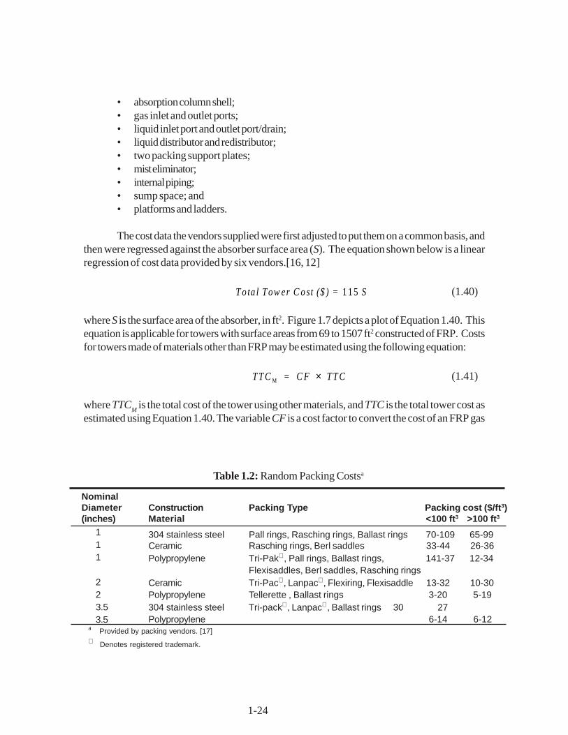
Table 1.2: Random Packing Costsa

Nominal Diameter Construction Packing Type Packing cost ($/ft3) (inches) Material <100 ft3 >100 ft3

1 304 stainless steel Pall rings, Rasching rings, Ballast rings 70-109 65-99 1 Ceramic Rasching rings, Berl saddles 33-44 26-36 1 Polypropylene Tri-Pak , Pall rings, Ballast rings, 141-37 12-34

Flexisaddles, Berl saddles, Rasching rings 2 Ceramic Tri-Pac , Lanpac , Flexiring, Flexisaddle 13-32 10-30 2 Polypropylene Tellerette , Ballast rings 3-20 5-19 3.5 304 stainless steel Tri-pack , Lanpac , Ballast rings 30 27 3.5 Polypropylene 6-14 6-12

a Provided by packing vendors. [17] Denotes registered trademark.

1-24

absorber to an absorber fabricated from another material. Ranges of cost factors provided by vendors are listed for the following materials of construction:[12]

304 Stainless steel: 1.10 - 1.75 Polypropylene: 0.80 - 1.10

Polyvinyl chloride: 0.50 - 0.90

Auxiliary costs encompass the cost of all necessary equipment not included in the absorption column unit. Auxiliary equipment includes packing material, instruments and controls, pumps, and fans. Cost ranges for various types of random packings are presented in Table 1.2. The cost of structured packings varies over a much wider range. Structured packings made of stainless steel range from $45/ft3 to $405/ft3, and those made of polypropylene range from $65/ft3 to $350/ft3.[17]

Similarly, the cost of instruments and controls varies widely depending on the complexity required. Gas absorber vendors have provided estimates ranging from $1,000 to $10,000 per column. A factor of 10 percent of the EC will be used to estimate this cost in this chapter. (see eq. 1.42, below.) Design and cost correlations for fans and pumps will be presented in a chapter on auxiliary equipment elsewhere in this manual. However, cost data for auxiliaries are available from the literature (see reference [18], for example).

The total equipment cost (EC) is the sum of the component equipment costs, which includes tower cost and the auxiliary equipment cost.

E C = T T C + P ack ing C ost + A ux ilia ry E qu ipm en t (1.42)

The purchased equipment cost (PEC) includes the cost of the absorber with packing and its auxiliaries (EC), instrumentation (0.10 EC), sales tax (0.03EC), and freight (0.05EC). The PEC is calculated from the following factors, presented in Section 1 of this manual and confirmed from the gas absorber vendor survey conducted during this study:[12, 19],

P E C = (1+ 0 .10+ 0 .03+ 0 .05)E C = 1.18 E C (1.43)

1.4.2 Installation Costs

The total capital investment,TCI, is obtained by multiplying the purchased equipment cost, PEC, by the total installation factor:

T C I = 2 .20 P E C (1.44)

The factors which are included in the total installation factor are also listed in Table 1.3.[19] The factors presented in Table 1.3 were confirmed from the gas absorber vendor survey.

1-25

1.5 Estimating Annual Cost

The total annual cost (TAC) is the sum of the direct and indirect annual costs.

1.5.1 Direct Annual Costs

Direct annual costs (DC) are those expenditures related to operating the equipment, such as labor and materials. The suggested factors for each of these costs are shown in Table 1.4. These factors were taken from Section 1 of this manual and were confirmed from the gas absorber vendor

The annual cost for each item is calculated by multiplying the number of units used annuallysurvey. (i.e., hours, pounds, gallons, kWh) by the associated unit cost.

Operating labor is estimated at ½-hour per 8-hour shift. The supervisory labor cost is estimated at 15 percent of the operating labor cost. Maintenance labor is estimated at 1/2-hour per 8-hour shift. Maintenance materials costs are assumed to equal maintenance labor costs.

Solvent costs are dependent on the total liquid throughput, the type of solvent required, and the fraction of throughput wasted (often referred to as blow-down). Typically, the fraction of solvent wasted varies from 0.1 percent to 10 percent of tire total solvent throughput.[12] For acid gassystems, the amount of solvent wasted is determined by the solids content, with bleed off occurringwhen solids content reaches 10 to 15 percent to prevent salt carry-over.[12]

The total annual cost of solvent (Cs) is given by:

annua l

so lven t m in

C = L W Fs i 60 opera ting (1.45)un it co st h r hours

where WF is the waste (make-up) fraction, and the solvent unit cost is expressed in terms of $/gal.

The cost of chemical replacement (Cc) is based on the annual consumption of the chemical

and can be calculated by:

annua l

opera ting

hours

chem ica l

where the chemical unit cost is in terms of $/lb.

c h r

lb s chem ica l u sed

C = (1.46)un it co st

1-26

Table 1.3: Capital Cost Factors for Gas Absorbers [19]

Cost Item Factor

Direct Costs Purchased equipment costs

Absorber + packing + auxiliary equipment a , EC As estimated, A Instrumentation b 0.10 A Sales taxes 0.03 A Freight 0.05 A

Purchased equipment cost, PEC B = 1.18 A

Direct installation costs Foundations & supports 0.12 B Handling & erection 0.40 B Electrical 0.01 B Piping 0.30 B Insulation 0.01 B Painting 0.01 B

Direct installation costs 0.85 B

Site preparation As required, SP Buildings As required, Bldg.

Total Direct Costs, DC 1.85 B + SP + Bldg.

Indirect Costs (installation) Engineering 0.10 B Construction and field expenses 0.10 B Contractor fees 0.10 B Start-up 0.01 B Performance test 0.01 B Contingencies 0.03 B

Total Indirect Costs, IC 0.35 B

Total Capital Investment = DC + IC 2.20 B + SP + Bldg.

a Includes the initial quantity of packing, as well as items normally not included with the unit supplied by vendors, such as ductwork, fan, piping, etc. b Instrumentation costs cover pH monitor and liquid level indicator in sump.

1-27

c

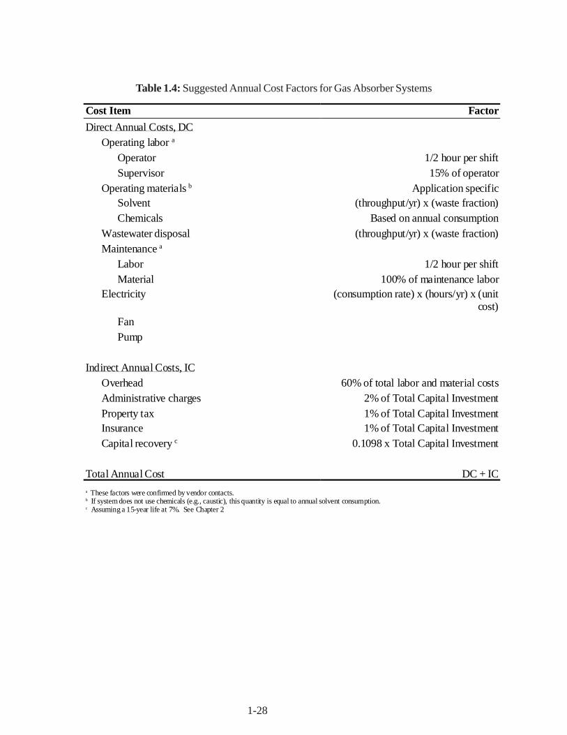
Table 1.4: Suggested Annual Cost Factors for Gas Absorber Systems

Cost Item Factor

Direct Annual Costs, DC Operating labor a

Operator 1/2 hour per shift Supervisor 15% of operator

Operating materials b Application specific Solvent (throughput/yr) x (waste fraction) Chemicals Based on annual consumption

Wastewater disposal (throughput/yr) x (waste fraction) Maintenance a

Labor 1/2 hour per shift Material 100% of maintenance labor

Electricity (consumption rate) x (hours/yr) x (unit cost)

Fan Pump

Indirect Annual Costs, IC Overhead 60% of total labor and material costs Administrative charges 2% of Total Capital Investment Property tax 1% of Total Capital Investment Insurance 1% of Total Capital Investment Capital recovery c 0.1098 x Total Capital Investment

Total Annual Cost DC + IC a These factors were confirmed by vendor contacts. b If system does not use chemicals (e.g., caustic), this quantity is equal to annual solvent consumption.

Assuming a 15-year life at 7%. See Chapter 2

1-28

Solvent disposal (Cww

) costs vary depending on geographic location. type of waste disposed of, and availability of on-site treatment. Solvent disposal costs are calculated by:

annua l

opera ting

hours

so lven t m in

60C = L W F (1.47)i d isposa l cos hrw w t

where the solvent disposal costs are in terms of $/gal of waste solvent.

The electricity costs associated with operating a gas absorber derive from fan requirements to overcome the pressure drop in the column, ductwork, and other parts of the control system, and pump requirements to recirculate the solvent. The energy required for the fan can be calculated using Equation 1.48:

10 41.17 × G i D P (1.48)E nergy fan =

ε

where Energy (in kilowatts) refers to the energy needed to move a given volumetric flow rate of air (acfm), G

i is the waste gas flow rate entering the absorber, P is the total pressure drop through the

system (inches of H2O) and is the combined fan-motor efficiency. Values for typically range from

0.4 to 0.7. Likewise, the electricity required by a recycle pump can be calculated using Equation 1.49:

× (0 .746 ) (2 .52 10 -1 ) Li (p ressure)

where 0.746 is the factor used to convert horsepower to kW, pressure is expressed in feet of water, and is the combined pump-motor efficiency.

The cost of electricity (Ce) is then given by:

E nergy pum p = (1.49)ε

annua l

opera ting

hours

cost o f

C e = E nergy fan + pum p (1.50)elec tr ic ity

where cost of electricity is expressed in units of $/KW-hr.

1.5.2 Indirect Annual Costs

Indirect annual costs (IC) include overhead, taxes, insurance, general and administrative (G&A), and capital recovery costs. The suggested factors for each of these items also appear in

1-29

Table 1.4. Overhead is assumed to be equal to 60 percent of the sum of operating, supervisory, and maintenance labor, and maintenance materials. Overhead cost is discussed in Section 1 of this manual.

The system capital recovery cost, CRC, is based on an estimated 15-year equipment life. (See Section 1 of this manual for a discussion of the capital recovery cost.) For a 15-year life and an interest rate of 7 percent, the capital recovery factor is 0.1098 The system capital recovery cost is then estimated by:

C R C = 0 .1098 T C I (1.51)

G&A costs, property tax, and insurance are factored from total capital investment, typically at 2 percent, 1 percent, and 1 percent, respectively.

1.5.3 Total Annual Cost

Total annual cost (TAC) is calculated by adding the direct annual costs and the indirect annual costs.

T A C = D C + IC (1.52)

1.6 Example Problem

The example problem presented in this section shows how to apply the gas absorber sizing and costing procedures presented in this chapter to control a waste gas stream consisting of HCl and air. This example problem will use the same outlet stream parameters presented in the thermal incinerator example problem found in Section 3.2, Chapter 2 of this manual. The waste gas stream entering the gas absorber is assumed to be saturated with moisture due to being cooled in the quench chamber. The concentration of HCl has also been adjusted to account for the change in volume.

1.6.1 Required Information for Design

The first step in the design procedure is to specify the conditions of the gas stream to be controlled and the desired pollutant removal efficiency. Gas and liquid stream parameters for this example problem are listed in Table 1.5.

The quantity of HCl can be written in terms of lb-moles of HCl per lb-moles of pollutant-free-gas (Y

i) using the following calculation:

0.001871 lb − m oles H C L Yi = = 0.00187

1 − 0.001871 lb - m o le po llu tan t free gas

1-30

The solvent, a dilute aqueous solution of caustic, is assumed to have the same physical properties as water.

1.6.2 Determine Gas and Liquid Stream Properties

Once the properties of the waste gas stream entering the absorber are known. the properties of the waste gas stream exiting the absorber and the liquid streams entering and exiting the absorber need to be determined. The pollutant concentration in the entering liquid (X

i) is assumed to be zero.

The pollutant concentration in the exiting gas stream (Y ) is calculated using Equation 1.1 and ao

removal efficiency of 99 percent.

Yo = 0 00187 1. −

99 100

= 0 0000187.

The liquid flow rate entering the column is calculated from theLs/G

s ratio using Equation 1.2.

Since Yi, Y

o, and X

i are defined, the remaining unknown, X

o*, is determined by consulting the

equilibrium curve. A plot of the equilibrium curve-operating line graph for an HCl-water system is presented in Figure 1.8. The value of X

o* is taken at the point on the equilibrium curve where Y

i

intersects the curve. The value of Yi intersects the equilibrium curve at an X value of 0.16.

lb-m

ole

HC

L/l

b-m

ole

Car

rier

Gas

0.002

0.0018

0.0016

0.0014

0.0012

0.001

0.0008

0.0006

0.0004

0.0002

0

(Xo,Yo)

Slo p e o f E quilibrium Curv e

Op erat in g L in e E quilibrium L in e

(Xi, Yo )

(Xo*,Yi)

0 0.02 0.04 0.06 0.08 0.1 0.12 0.14 0.16 0.18 0.2

lb -moles HCl/lb -mole Solvent

Figure 1.8: Equilibrium Curve Operating Line for the HCl-Water System [7]

1-31

Table 1.5: Example Problem Data

Parameters Values

Stream Properties

Waste Gas Flow Rate Entering Absorber 21,377 scfm (22,288 acfm)

Temperature of Waste Gas Stream 100oF

Pollutant in Waste Gas HCI

Concentration of HCl Entering Absorber in Waste Gas 1871 ppmv

Pollutant Removal Efficiency 99% (molar basis)

Solvent Water with caustic in solution

Density of Waste Gas a 0.0709 lb/ft3

Density of Liquid [7] 62.4 lb/ft3

Molecular Weight of Waste Gasa 29 lb/lb-mole

Molecular Weight of Liquid [7] 18 lb/lb-mole

Viscosity of Waste Gasa 0.044 lb/ft-hr

Viscosity of Liquid [7] 2.16 lb/ft-hr

Minimum Wetting Rate [7] 1.3 ft2/hr

Pollutant Properties b

Diffusivity of HCl in Air 0.725 ft2/hr

Diffusivity of HCl in Water 1.02 x 10-4 ft2/hr

Packing Properties c

Packing type 2-inch ceramic Raschig rings

Packing factor: Fp 65

Packing constant: � 3.82

Packing constant: � 0.41

Packing constant: � 0.45

Packing constant: � 0.0125

Packing constant: b 0.22

Surface Area to Volume Ratio 28

a Reference [7], at 100oF b Appendix 9A. c Appendix 9B.

1-32

The operating line is constructed by connecting two points: (X , Y ) and (X * , Y ). The slopei o o i

of the operating line intersecting the equilibrium curve, (Ls/G

s)min, is:

L 0.00187 − 0.0000187 s = = 0.0116 G s 0.16 − 0

m in

The actual Ls/G

s ratio is calculated using Equation 1.3. For this example, an adjustment

factor of 1.5 will be used.

m in lb(60 ) (0.0709 ) (22 ,288 acfm )3h r ft lb − m oles G s = = 3,263

lb h r(29 ) (1 + 0.00187 )lb −m ole

The flow rate of the solvent entering the absorber may then be calculated using Equation 1.5.

lb − m oles lb − m oles L s = 0.0174 3,263 = 56.8 h r h r

The values of G and L are calculated using Equations 1.6 and 1.7, respectively:mol,i mol,i

lb − m oles lb − m oles G m ol ,i = 3,263 (1 + 0.00187 ) = 3,269 h r h r

lb − m oles lb − m oles L m ol ,i = 56.8 (1 + 0 ) = 56.8 h r h r

The pollutant concentration exiting the absorber in the liquid is calculated using Equation 1.10.

0.00187 − 0.0000187 0 .106 lb − m oles H C L x o = =

0.0174 lb − m ole so lve n t

1-33

1.6.3 Calculate Absorption Factor

The absorption factor is calculated from the slope of the equilibrium line and the L /Gmol,i mol,i

ratio. The slope of the equilibrium curve is based on the mole fractions of x , x , y *, and y *, whichi o i o

are calculated fromXi, X

o, Y

i* andY

o* from Figure 1.8. From Figure 1.8, the value ofY

o* in equilibrium

with the Xo value of 0.106 is 0.0001. The values of Y

i* and Xi are 0. The mole fraction values are

calculated from the concentration values using Equations 1.13 through 1.16.

0.106 x o = = 0.096

1 + 0.106

* 0.0001 y o = = 0.0001

1 + 0.0001

The slope of the equilibrium fine from xi to x

o is calculated from Equation 1.12:

0 0001. − 0 m = = 0.00104

0.096 − 0

Since HCl is very soluble in water, the slope of the equilibrium curve is very small. The absorption factor is calculated from Equation 1.11.

0.0174 A F = = 17

0.00104

1.6.4 Estimate Column Diameter

Once the inlet and outlet stream conditions are determined, the diameter of the gas absorber may be calculated using the modified generalized pressure drop correlation presented in Figure 1.5. The Abscissa value from the graph is calculated from Equation 1.17:

18 0.0709 A bcissa = 0.0174 = 0.000364

29 62 .4

Since this value is outside the range of Figure 1.5, the smallest value (0.01) will be used as a default value. The Ordinate is calculated from Equation 1.19.

2[−1.668 −1.085(log 0 .01)−0 .297 (log 0 .01) ]O rd inate = 10 = 0.207

The superficial gas flow rate, G , is calculated using Equation 1.20. For this example calculation,sfr,i

1-34

2-inch ceramic Rasching rings are selected as the packing. The packing factors for Raching rings are listed in Appendix B.

=G sfr ,i

( ) ( ) ( ) ( ) ( ) ( ) ( )

sec

.

. . . .

. .=

− 0 207 62 4 0 0709 32 2

65 1 0 893 0 681

2

0 2

lb

ft

ft

2

3 lb

se c ft

Once G is determined, the cross-sectional area of the column is calculated usingsfr,i

Equation 1.21.

lb −m ol lb(3,263 ) (29 )hr lb −m ol A = = 55.1 ft 2

sec lb(3600 ) (0.681 ) (0.7 )hr sec −ft 2

The superficial liquid flow rate is determined using Equation 1.23.

lb −m ol lb(56.8 ) (18 )hr lb −m ol lb L sfr ,i = 2 = 18.6 255.1 ft h r − ft

At this point, it is necessary to determine if the liquid flow rate is sufficient to wet the packed bed. The minimum value ofL is calculated using Equation 1.24. The packing constant (a) is found

sfr,i

in Appendix B.

ft 2 lb ft 2 lb(L sfr ,i ) = 1.3 62.4 3 28 3 = 2 ,271 2m in h r ft ft h r − ft

The L value calculated using the L/G ratio is far below the minimum value needed to wet thesfr,i

packed bed. Therefore, the new value, (L ) will be used to determine the diameter of thesfr,i min

absorber. The calculations for this revised diameter are shown in Appendix C. Appendix C shows that the cross-sectional area of the column is calculated to be 60 ft2, L is 7572, and G is 0.627

mol,i sfr,i

lb/sec-ft2. (The diameter of the column is then calculated using Equation 1.22)

D = ( ) (4 60

Π

2ft )= 8 74. ft

The value of X is then: o

x o = 0 00187. − 0 0000187.

7 572, = 0 0008.

3 263,

1-35

Expressed in terms of mole fraction:

0.0008 x o = = 0.0008

1 − 0.0008

The value of yo in equilibrium with x

o cannot be estimated accurately. However, the value will

approach zero, and the value of AF will be extremely large:

7 ,572 A F = → ∞(3,263) (≈ 0 )

1.6.5 Calculate Column Surface Area

Since xi = 0 and AF is large, Equation 1.26 will be used to calculate the number of

transfer units:

0.00187 n tu = 1n = 4.61 0.0000187

The height of a transfer unit is calculated from , AF, H , and H . The values of H and H areL G G L

calculated from Equations 1.29 and 1.30:

0 .41

3.82[(3,600) (0.7 ) (0.627 )] 0.044 = = 2.24 ftH G 0 .452 ,271 (0.725) (0.0709 )

0 .22 2 ,271 2.16 H L = 0.0125 = 1.06 ft 2.16 (0.000102 ) (62 .4 )

The height of the transfer unit is calculated using Equation 1.28:

1 H tu = (2.24 ft ) +

∞(1 .06 ft ) = 2 .24 ft

1-36

The depth of packing is calculated from Equation 1.25.

H = N tu × H = (4 .61) (2 .24 ft ) = 10 .3 ftpack tu

The total height of the column is calculated from Equation 1.33:

H = 1.40 (10.3) + 1.02 (8 .74 ) + 2 .81 = 26 .1 fttow er

The surface area of the column is calculated using Equation 1.34:

8 .74 s = ( . ) (8 .74 26 .1 + = 836 ft 23 14 )

2

1.6.6 Calculate Pressure Drop

The pressure drop through the column is calculated using Equation 1.35.

(0 .17 ) (2 ,271) [(0.7 ) (0.627 )]2

3 ,600∆P = (0 .24 ) 10 0.0709

= 0.83 inches water/foot packing

The total pressure drop (through 10.3 feet of packing) equals 8.55 inches of water.

1.6.7 Equipment Costs

Once the system sizing parameters have been determined, the equipment costs can be calculated. For the purpose of this example, a gas absorber constructed of FRP will be costed using Equation 1.40.

TTC($) = 115(836) = $96,140

The cost of 2-inch ceramic Raschig rings can be estimated from packing cost ranges presented in Section 1.5. The volume of packing required is calculated as:

Volume of packing = (60 ft2)(10.3 ft) = 618 ft3

Using the average of the cost range for 2-inch ceramic packings, the total cost of packing is:

1-37

Packing cost = ($20/ft3)(618 ft3) = $12,360

For this example problem, the cost of a pump will be estimated using vendor quotes. First, the flow rate of solvent must be converted into units of gallons per minute:

lb 2 gal h r L (gpm ) = 2 ,271 2 (60 ft ) = 272 gpm h - ft 8 .34 lb 60 m in

The average price for a FRP pump of this size is $16/gpm at a pressure of 60 ft water, based on the vendor survey.[12] Therefore, the cost of the recycle pump is estimated as:

$16 C pum p = (272 gpm )

gpm

= $4 ,350 gpm

For this example, the cost for a fan (FRP, backwardly-inclined centrifugal) can be calculated using the following equation:[18]

1.38C fan = 57 .9 d

where d is the impeller (wheel) diameter of the fan expressed in inches. For this gas flow rate and pressure drop, an impeller diameter of 33 inches is needed. At this diameter, the cost of the fan is:

0 .821 C 104 ( )= hp m otor

The cost of a fan motor (three-phase, carbon steel) with V-belt drive, belt guard, and motor starter can be computed as follows:[18]

0 .821C m otor = 104 (42.6 ) = $2 ,260

As will be shown in Section 1.6.8, the electricity consumption of the fan is 32.0kW. Converting to horsepower, we obtain a motor size of 42.6 hp. The cost of the fan motor is:

(1.17 × 10 −4 ) (22 ,288) (8.55)E nergy fan = = 32.0 kw

0.70

The total auxiliary equipment cost is:

1-38

$4,350 + $7,210 + $2,260 = $13,820

The total equipment cost is the sum of the absorber cost, the packing cost, and the auxiliary equipment cost:

EC = 96,140 + 12,360 + 13,820 = $122,320

The purchased equipment cost including instrumentation, controls, taxes, and freight is estimated using Equation 1.43:

PEC = 1.18(122,320) = $144,340

The total capital investment is calculated using Equation 1.44:

TCI = 2.20(144,340) = $317,550 $318,000

1.6.8 Total Annual Cost

Table 1.6 summarizes the estimated annual costs using the suggested factors and unit costs for the example problem.

Direct annual costs for gas absorber systems include labor, materials, utilities, and wastewater disposal. Labor costs are based on 8,000 hr/year of operation. Supervisory labor is computed at 15 percent of operating labor, and operating and maintenance labor are each based on 1/2 hr per 8-hr shift.

The electricity required to run the fan is calculated using Equation 1.48 and assuming a combined fan-motor efficiency of 70 percent:

−4(1.17 × 10 ) (22 ,288 ) (8.55)E nergy fan = = 32.0 kw

0.70

The energy required for the liquid pump is calculated using Equation 1.49. The capital cost of the pump was calculated using data supplied by vendors for a pump operating at a pressure of 60 feet of water. Assuming a pressure of 60 ft of water a combined pump-motor efficiency of 70 percent:

−4(0.746) (2.52 × 10 ) (272 ) (60 ) ( )1 E nergy pum p = = 4.4 kw

0.70

The total energy required to operate the auxiliary equipment is approximately 36.4 kW.

1-39

Table 1.6: Annual Costs for Packed Tower Absorber Example Problem

Cost Item Calculations Cost

Direct Annual Costs, DC

Operating Labor 0.5hr x shift x 8,000hr x $15.64 $7,820 Operator shift 8hr yr hr

Supervisor 15% of operator = 0.15 × 7,820 1,170

Operating materials Solvent (water) 7.16 gpm x 60 min x 8,000hr x $0.20 690

hr yr 1000gal

Caustic Replacement 3.06lb-mole x 62lb x 8,000hr x ton x 1 x $300 299,560 hr lb-mole yr 2000lb 0.76 ton

Wastewater disposal 7.16gpm x 60 min x 8,000 hr x $3.80 13,060 hr yr 100gal

Maintenance Labor 0.5 x shift x 8,000hr x $17.21 8,610

shift 8hr yr hr

Material 100% of maintenance labor 8,610

Electricity 36.4kw x 8,000hr $0.0461 13,420 yr kWh

Total DC $352,940

Indirect Annual Costs, IC

Overhead 60% of total labor and maintenance material: 15,730 = 0.6(7,820 + 1,170 + 8,610 + 8,610)

Administrative charges 2% of Total Capital Investment = 0.02($317,550) 6,350 Property tax 1% of Total Capital Investment = 0.01($317,550) 3,180 Insurance 1% of Total Capital Investment = 0.01($317,550) 3,180

Capital recoverya 0.1315 × $317,550 41,760

Total IC $70,200

Total Annual Cost (rounded) $423,000

a The capital recovery cost factor, CRF, is a function of the absorber equipment life and the opportunity cost of the capital (i.e., interest rate). For this example, assume a 15-year equipment life and a 10% interest rate.

1-40

The cost of electricity, Ce, is calculated using Equation 1.50 and with the cost per kWh

shown in Table 1.6.

Ce = (36.4kW)(8,000 h/yr)($0.0461/kWh) = $13,420/yr

The costs of solvent (water), wastewater disposal, and caustic are all dependent on the total system throughput and the fraction of solvent discharged as waste. A certain amount of solvent will be wasted and replaced by a fresh solution of water and caustic in order to maintain the system’s pH and solids content at acceptable levels. Based on the vendor survey, a maximum solids content of 10 percent by weight will be the design basis for this example problem.[12] The following calculations illustrate the procedure used to calculate how much water and caustic are needed, and how much solvent must be bled off to maintain system operability.

From previous calculations, L = 7,572 lb-moles/hr. The mass flow rate is calculated as:mol,i

lb − m ole lb lb =

With G at 3,263 lb-moles/hr, the mass flow rate of the gas stream is calculated as:mol,i

7 ,572 18 136,300L = −m ass h r lb m o le h r

lb − m ole lb lb

=

The amount of HCl in the gas stream is calculated on a molar basis as follows:

=

3,263 29 94 ,800G = −m ass h r lb m o le h r

lb − m ole

lb - m o lH C L ppm v

3,263 1874 6.12G = H C L 6m ass , h r h r1 10×

On a mass basis:

=

For this example problem, the caustic is assumed to be Na2O, with one mole of caustic required for

neutralizing 2 moles of HCl. Therefore, 3.06 lb-moles/hr of caustic are required.

lb - m o lH C L

lb lb H C L

6.12 36.5 223.4G = m ass , H C L h r lb - m o le h r

1-41

_____________________

The unit cost of a 76 percent solution of Na2O is given in Table 1.6. The annual cost is

calculated from:

C c = 3 06. lb - m o le s

h r

62 lb

lb - m o le

8 ,000 y r

h r

to n

2 ,000

lb

1 0 76.

$300 to n

= $299 ,560 y r

Mass of the salt formed in this chemical reaction, NaC1, is calculated as:

M ass N aC l = 223 4. lb - H C L

h r 3

lb

6 .5

- m o le

lb H C L

1 lb lb -

- m o le N aC l

m o le H C L

58 5.

lb - m

lb N a C l

o le N aC l lb N aC l

= 358.1 h r

If the maximum concentration of NaC1 in the wastewater (ww) is assumed to be 10 weight percent, the wastewater volume flow rate is calculated as:

lb N aC l 1 lb w w gal w w 1 h r W astew a ter flow ra te = 358.1 h r 0 .1 lb N aC l 8 .34 lb w w 60 m in

= 7.16 gpm

where 8.34 is the density of the wastewater.

The cost of wastewater disposal is:1

60 m in h r $3.80 $13,060 C w w = (7.16 gpm ) 8 ,000 =

lh r y r 1,000 gal y r

The cost of solvent (water) is:

60 m in h r $0.20 $690 C s = (7.16 gpm ) 8 ,000 =

lh r y r 1,000 gal y r

1Because the wastewater stream contains only NaC1, it probably will not require pretreatment before discharge to a municipal wastewater treatment facility. Therefore, the wastewater disposal unit cost shown here is just a sewer usage rate. This unit cost ($3.80/1,000 gal) is the average of the rates charged by the seven largest municipalities in North Carolina.[20] These rates range from approximately $2 to $6/1,000 gal. This wide range is indicative of the major differences among sewer rates throughout the country. Indirect annual costs include overhead, administrative charges, property tax, insurance, and capital recovery. Total annual cost is estimated using Equation 1.52. For this example case, the total annual cost is estimated to be

$423,000 per year (Table 1.6).

1-42

1.7

1.6.9 Alternate Example

In this example problem the diameter of a gas absorber will be estimated by defining a pressure drop. A pressure drop of 1 inch of water per foot of packing will be used in this example calculation. Equation 1.38 will be used to calculate the ordinate value relating to an abscissa value. If the L /G ratio is known, the Abscissa can be calculated directly. The Ordinate value is

mol, i mol,i

then:

Ordinate = exp [-4.0950-1.00121n(0.0496)-0.1587(1n 0.0496)2 + 0.0080(1n 0.0496)3 + 0.0032(1n 0.0496)4]

= 0.084

The value of Gsfr

is calculated using Equation 1.39.

(62.4 − 0.0709 ) (0.0709 ) (32.2 ) (0.084 ) lb G sfr ,i = 0 .1 = 0.43 265 (0.893) ft − sec

The remaining calculations are the same as in Section 1.3.4, except the flooding factor is not used in the equations.

Acknowledgments

The authors gratefully acknowledge the following companies for contributing data to this chapter:

� Air Plastics, Inc. (Cincinnati, OH) � April, Inc. (Teterboro, NJ) � Anderson 2000, Inc. (Peachtree City, GA) � Calvert Environmental (San Diego, CA) � Ceilcote Air Pollution Control (Berea, OH) � Croll-Reynolds Company, Inc. (Westfield, NJ) � Ecolotreat Process Equipment (Toledo, OH) � Glitsch, Inc. (Dallas, TX) � Interel Corporation (Englewood, CO) � Jaeger Products, Inc. (Spring, TX) � Koch Engineering Co., Inc. (Wichita, KS) � Lantec Products, Inc. (Agoura Hills, CA) � Midwest Air Products Co., Inc. (Owosso, MI) � Monroe Environmental Corp., (Monroe, MI) � Norton Chemical Process Products (Akron, OH)

1-43

References

[1] Control Technologies for Hazardous Air Pollutants, Office of Research and Development, U.S. Environmental Protection Agency, Research Triangle Par,, North Carolina, Publication No. EPA 625/6-91-014.

[2] McInnes, R., K. Jameson, and D. Austin, “Scrubbing Toxic Inorganics”, Chemical Engineering, September 1990, pp. 116-121.

[3] Letter from Jose L. Bravo of Jaeger Products, Inc., to William M. Vatavuk, U. S. Environmental Protection Agency, June 8, 1992.

[4] Treybal, Robert E., Mass Transfer Operations (Third edition), McGraw-Hill Book Company, New York, 1980.

[5] Letter from Jack D. Brady of Anderson 2000, Inc., to William M. Vatavuk, U.S. Environmental Protection Agency, June 9, 1992.

[6] Letter from S. Raymond Woll of Air Products, Inc., to William M. Vatavuk, U.S. Environmental Protection Agency, June 25, 1992.

[7] Perry, R.H. and C.H. Chilton, Eds., Chemical Engineers’ Handbook (Sixth edition), McGraw-Hill Book Company, New York, 1984.

[8] Crowe, Charles R., and D. Cooper, “Brick/Membrane Linings Pass the Acid Test”, Chemical Engineering, July 1988, pp. 83-86.

[9] Harrison, Mark E., and John J. France, “Distillation Column Troubleshooting, Part 2: Packed Columns”, Chemical Engineering, April 1989, pp. 121-128.

[10] Coker, A.K., “Understanding the Basics of Packed-Column Design”, Chemical Engineering Progress, November 1991, pp. 93-99.

[11] Telephone conversation between Roy Oommen, Radian Corporation and Gerald Nealon, Norton Process Equipment, April 4, 1992.

[12] Gas absorber questionnaire responses from nine gas absorber vendors to Radian Corporation August-December, 1991.

[13] Buonicore, A.J., and L. Theodore, Industrial Control Equipment for Gaseous Pollutants, Volume I, CRC Press, Inc., Cleveland, Ohio, 1975.

1-44

[14] Strigle, Ralph F., Random Packings and Packed Towers, Design Applications, Gulf Publishing Company, Houston, Texas, 1987.

[15] Questionnaire response from K.C. Lang of Lantec Products, Inc. To R.V. Oommen, Radian Corporation, August 23, 1991.

[16] Memorandum from Vatavuk, W.M. of U.S. Environmental Protection Agency to Martha Smith, U.S. EPA, March 27, 1992.

[17] Packing vendor questionnaire responses from seven packing vendors to Radian Corporation, August 1991 - January 1992.

[18] Vatavuk, W.M., “Pricing Equipment for Air-Pollution Control”, Chemical Engineering, May 1990, pp. 126-130.

[19] Vatavuk, W.M., and R.B. Neveril, “Estimating Costs of Pollution Control Systems, Part II: Factors for Estimating Capital and Operating Costs”, Chemical Engineering, November 3, 1980, pp. 157-162.

[20] Telephone conversation between William M. Vatavuk, U.S. Environmental Protection Agency, and Cindy Kling, City of Raleigh, N.C., July 16, 1992.

[21] “Air Pollution Engineering Manual” (AP-40), (Second Edition), Danielson, John A., Los Angeles County Air Pollution Control District, CA, May 1973.

For information on escalating these prices to more current dollars, refer to the EPA report Escalation Indexes for Air Pollution Control Costs and updates thereto, all of which are installed on the OAQPS Technology Transfer Network (CTC Bulletin Board).

1-45

1

Appendix A

Properties of Pollutants

1-46

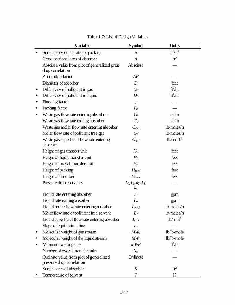
Table 1.7: List of Design Variables

Variable Symbol Units � Surface to volume ratio of packing a ft2/ft3

Cross-sectional area of absorber A ft2

Abscissa value from plot of generalized press Abscissa — drop correlation Absorption factor AF — Diameter of absorber D feet

� Diffusivity of pollutant in gas DG ft2/hr � Diffusivity of pollutant in liquid DL ft2/hr � Flooding factor f — � Packing factor Fp — � Waste gas flow rate entering absorber Gi acfm

Waste gas flow rate exiting absorber Go acfm Waste gas molar flow rate entering absorber Gmol lb-moles/h Molar flow rate of pollutant free gas Gs lb-moles/h Waste gas superficial flow rate entering Gsfr,i lb/sec-ft2

absorber Height of gas transfer unit HG feet Height of liquid transfer unit HL feet Height of overall transfer unit Htu feet Height of packing Hpack feet Height of absorber Htower feet Pressure drop constants k0, k1, k2, k3, —

k4

Liquid rate entering absorber Li gpm Liquid rate exiting absorber Lo gpm Liquid molar flow rate entering absorber Lmol,i lb-moles/h Molar flow rate of pollutant free solvent L? lb-moles/h Liquid superficial flow rate entering absorber Lsfr,i lb/hr-ft2

Slope of equilibrium line m — � Molecular weight of gas stream MWG lb/lb-mole � Molecular weight of the liquid stream MWL lb/lb-mole � Minimum wetting rate MWR ft2/hr

Number of overall transfer units Ntu — Ordinate value from plot of generalized Ordinate — pressure drop correlation Surface area of absorber S ft2

� Temperature of solvent T K

1-47

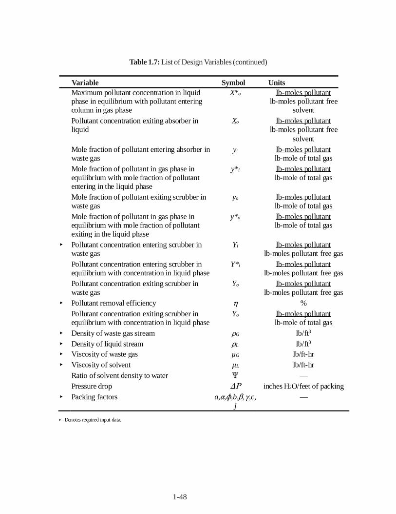
Table 1.7: List of Design Variables (continued)

Variable Symbol Units Maximum pollutant concentration in liquid X*o lb-moles pollutant phase in equilibrium with pollutant entering lb-moles pollutant free column in gas phase solvent Pollutant concentration exiting absorber in Xo lb-moles pollutant liquid lb-moles pollutant free

solvent Mole fraction of pollutant entering absorber in yi lb-moles pollutant waste gas lb-mole of total gas Mole fraction of pollutant in gas phase in y*i lb-moles pollutant equilibrium with mole fraction of pollutant entering in the liquid phase

lb-mole of total gas

Mole fraction of pollutant exiting scrubber in yo lb-moles pollutant waste gas lb-mole of total gas Mole fraction of pollutant in gas phase in y*o lb-moles pollutant equilibrium with mole fraction of pollutant exiting in the liquid phase

lb-mole of total gas

Pollutant concentration entering scrubber in Yi lb-moles pollutant waste gas lb-moles pollutant free gas Pollutant concentration entering scrubber in Y*i lb-moles pollutant equilibrium with concentration in liquid phase lb-moles pollutant free gas Pollutant concentration exiting scrubber in Yo lb-moles pollutant waste gas lb-moles pollutant free gas Pollutant removal efficiency � % Pollutant concentration exiting scrubber in Yo lb-moles pollutant equilibrium with concentration in liquid phase lb-mole of total gas Density of waste gas stream �G lb/ft3

Density of liquid stream �L lb/ft3

Viscosity of waste gas µG lb/ft-hr Viscosity of solvent µL lb/ft-hr Ratio of solvent density to water � — Pressure drop �� inches H2O/feet of packing Packing factors a,�,�,b, ,�,c, —

j

�

�

� � � �

�

� Denotes required input data.

1-48

Table 1.8: Physical Properties of Common Pollutantsa

Pollutant Molecular Diffusivity in Diffusivity in Weight Air Water

lb lb − m o le

at 25°C (cm2/sec)

at 20°C (cm2/sec)x105

Ammonia 17 0.236 1.76 Methanol 32 0.159 1.28 Ethyl Alcohol 46 0.119 1.00 Propyl Alcohol 60 0.100 0.87 Butyl Alcohol 74 0.09 0.77 Acetic Acid 60 0.133 0.88 Hydrogen Chloride 36 0.187 2.64 Hydrogen Bromide 36 0.129 1.93 Hydrogen Fluoride 20 0.753 3.33

a Diffusivity data taken from Reference [7, 21].

1-49

Appendix B

Packing Characteristics

1-50

Table 1.9: Packing Factors for Various Packings[3,7,10,13]

Nominal Packing

Type Construction

Level Diameter (inches)

Fp a

Raschig rings ceramic 1/2 5/8 3/4 1

640 380 255 160

111 100 80 58

1 1/2 2

95 65

38 28

3 37

Raschig rings metal 1/2 5/8 3/4 1

410 290 230 137

118

72 57

1 1/2 2

83 57

41 31

3 32 21

Pall rings metal 5/8 1

70 48

131 66

1 1/2 2

28 20

48 36

3 1/2 16

Pall rings polypropylene 5/8 1

97 52

110 63

1 1/2 2

32 25

39 31

Berl saddles ceramic 1/2 3/4 1

240 170 110

142 82 76

1 1/2 2

65 45

44 32

Intalox saddles ceramic 1/2 3/4 1

200 145 98

190 102 78

1 1/2 2

52 40

60 36

3 22

Tri-Packs® plastic 2 3 1/2

16 12

48 38

1-51

a

sfr sfr

a

asfr

Table 1.10: Packing Constants Used to Estimate HG [1, 3, 7, 13]

Packing Size Packing Constants Applicable Rangea

Type (inches) � � � Gsfr Lsfr

Raschig Rings

3/8 1 1

1 1/2 1 1/2

2

2.32 7.00 6.41 1.73 2.58 3.82

0.45 0.39 0.32 0.38 0.38 0.41

0.47 0.58 0.51 0.66 0.40 0.45

200-500 200-800 200-600 200-700 200-700 200-800

500-1,500 400-500

500-4,500 500-1,500

1,500-4,500 500-4,500

Berl Saddles 1/2 1/2 1

1 1/2

32.4 0.81 1.97 5.05

0.30 0.30 0.36 0.32

0.74 0.24 0.40 0.45

200-700 200-700 200-800

200-1,000

500-1,500 1,500-4,500 400-4,500 400-4,500

Partition Rings

3 640 0.58 1.06 150-900 3,000-10,000

LanPac® 2.3 7.6 0.33 -0.48 400-3,000 500-8,000

Tri-Packs® 2 3 1/2

1.4 1.7

0.33 0.33

0.40 0.45

100-900 100-2,000

500-10,000 500-10,000

aUnits of lb/hr-ft2

Table 1.11: Packing Constants Used to Estimate HL [1, 3, 13]

Packing Type

Size (inches)

Packing Constants

� b

Applicable Rangea

Lasfr

Raschig Rings 3/8 1

1 1/2 2 1/2

2

0.00182 0.00357 0.0100 0.0111 0.0125

0.46 0.35 0.22 0.22 0.22

400-15,000 400-15,000 400-15,000 400-15,000 400-15,000

Berl Saddles 1/2 1

1 1/2

0.00666 0.00588 0.00625

0.28 0.28 0.28

400-15,000 400-15,000 400-15,000

Partition Rings 3 0.0625 0.09 3,000-14,000

LanPac® 2.3 3.5

0.0039 0.0042

0.33 0.33

500-8,000 500-8,000

Tri-Packs® 2 0.0031 0.33 500-10,000 3 1/2 0.0040 0.33 500-10,000

aUnits of lb/hr-ft2

1-52

Table 1.12: Packing Constants Used to Estimate Pressure Drop [1, 7, 13]

Nominal Packing

Type Construction

Material Diameter (inches)

c j

Raschig rings ceramic 1/2 3/4 1

3.1 1.34 0.97

0.41 0.26 0.25

1 1/4 1 1/2

2

0.57 0.39 0.24

0.23 0.23 0.17

Raschigrings metal 5/8 1

1.2 0.42

0.28 0.21

11/2 2

0.29 0.23

0.20 0.135

Pallrings metal 5/8 1

0.43 0.15

0.17 0.16

11/2 2

0.08 0.06

0.15 0.12

Berlsaddles ceramic 1/2 3/4 1

1.2 0.62 0.39

0.21 0.17 0.17

11/2 0.21 0.13

Intaloxsaddles ceramic 1/2 3/4 1

0.82 0.28 0.31

0.20 0.16 0.16

11/2 0.14 0.14

1-53

Appendix C

Minimum Wetting Rate Analysis

1-54

Minimum Wetting Rate Analysis

As explained in the design procedures, the liquid flow rate entering the column must be high enough to effectively wet the packing. If the liquid flow rate, as determined theoretically in Equation 1.23, is lower than the flow rate dictated by the minimum wetting rate, calculated in Equation 1.24, then the packing will not be wetted sufficiently to ensure mass transfer between the gas and liquid phases. The minimum liquid flow rate should then be used as a default value. The superficial gas flow rate, G

sfr, , and cross-sectional area of the column must then be recalculated to account for the

increased liquid flow rate. The approach is outlined below

� The value of L must be recalculated from the value of (L ) using the equation:mol,i sfr,i min

(L ) Asfr ,i

L = m in m ol ,i ( M W ) L

The value of A (the cross-sectional area of the absorber column) is the only unknown in the equation.

� The Abscissa value is calculated in terms of A by substituting the new L intomol,i

Equation 1.17.

� The value of G is recalculated by rearranging Equation 1.21, with A as the onlysfr,i

unknown.

� The Ordinate value is calculated in terms of A from the new G using the Equation 1.18.sfr,i

� An iterative process is used to determine A, Abscissa, and Ordinate. Values of A are chosen and the Abscissa and Ordinate values are calculated. The Ordinate value corresponding to the Abscissavalue is determined from Figure 1.5 (or Equation .19), and this value is compared to the Ordinate value calculated using Equation 1.18. This process is continued until both Ordinate values are equal.

Step 1: The first step is to recalculate the liquid flow rate. The liquid molar flow rate may be calculated using Equation 1.23.

lb lb − m ole lb − m ole L m ol ,i = 2 ,271 2 A = 126.2 2 A

h r − ft 18 lb h r − ft

1-55

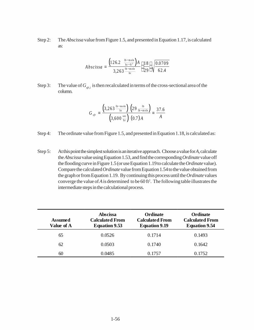
Step 2: The Abscissa value from Figure 1.5, and presented in Equation 1.17, is calculated as:

lb −m ole 2(126.2 hr −ft )A 18 0.0709

A bscissa = lb −m ole 3,263 29 62.4 hr

Step 3: The value of G is then recalculated in terms of the cross-sectional area of thesfr,i

column.

lb −m ole lb(3,263 ) (29 lb − ) 37 6hr m ole . G sfr = =

sec A(3,600 ) (0.7 ) Ahr

Step 4: The ordinate value from Figure 1.5, and presented in Equation 1.18, is calculated as:

Step 5: Atthis point the simplest solution is an iterative approach. Choose a value forA, calculate the Abscissa value using Equation 1.53, and find the corresponding Ordinate value off the flooding curve in Figure 1.5 (or use Equation 1.19 to calculate the Ordinate value). Compare the calculatedOrdinate value from Equation 1.54 to the value obtained from the graph or from Equation 1.19. By continuing this process until the Ordinate values converge the value of A is determined to be 60 ft2. The following table illustrates the intermediate steps in the calculational process.

Assumed Value of A

Abscissa Calculated From

Equation 9.53

Ordinate Calculated From

Equation 9.19

Ordinate Calculated From

Equation 9.54

65 0.0526 0.1714 0.1493

62 0.0503 0.1740 0.1642

60 0.0485 0.1757 0.1752

1-56

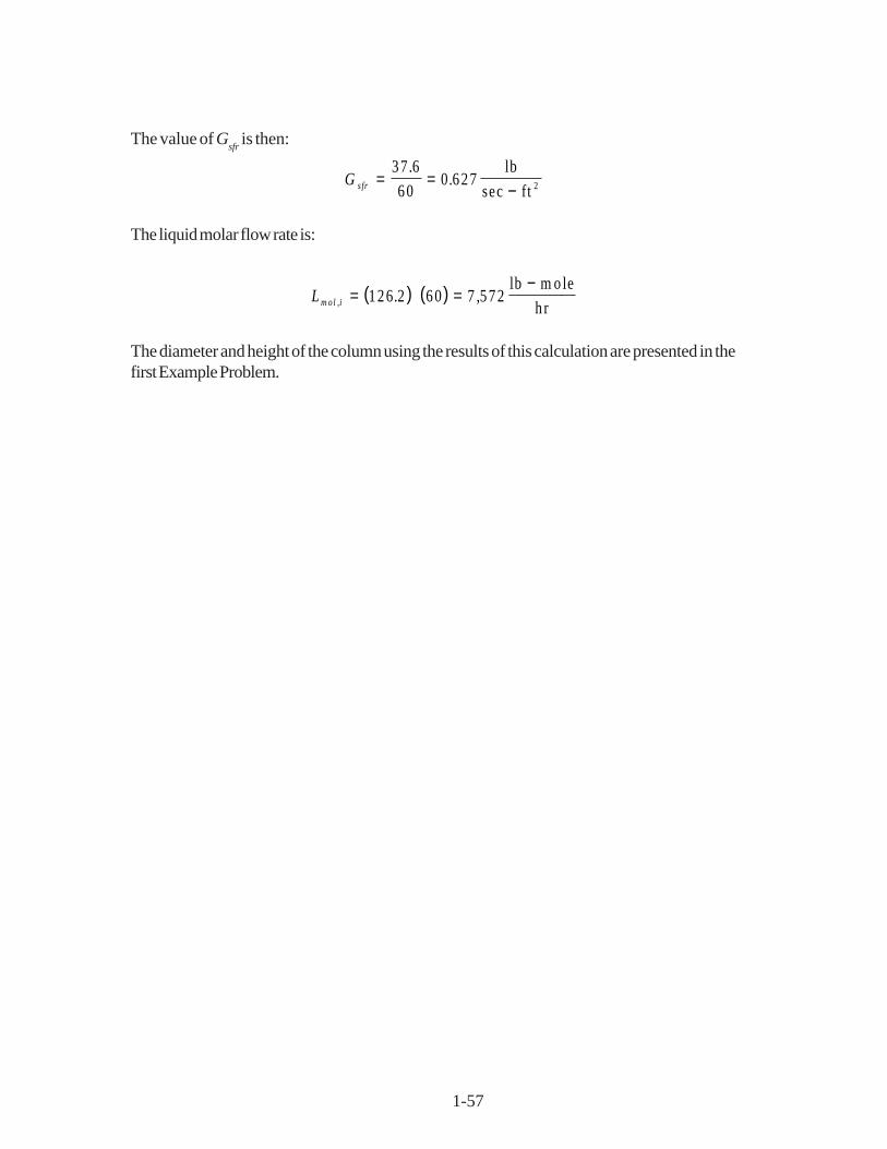
The value of Gsfr

is then:

G sfr = 37 6.

60 = 0 627.

lb

se c − ft 2

The liquid molar flow rate is:

lb − m o le L m ol ,i = (126.2 ) (60 ) = 7 ,572

h r

The diameter and height of the column using the results of this calculation are presented in the first Example Problem.

1-57

EPA Form 2220- Rev. 4-77)

TECHNICAL REPORT DATA (Please read Instructions on reverse before completing)

1. REPORT NO.

452/B-02-001 2. 3. RECIPIENT'S ACCESSION NO.

4. TITLE AND SUBTITLE

The EPA Air Pollution Control Cost Manual

5. REPORT DATE

January, 2002 6. PERFORMING ORGANIZATION CODE

7. AUTHOR(S)

Daniel Charles Mussatti 8. PERFORMING ORGANIZATION REPORT NO.

9. PERFORMING ORGANIZATION NAME AND ADDRESS

U.S. Environmental Protection Agency Office of Air Quality Planning and Standards Air Quality Standards and Strategies Division Innovative Strategies and Economics Group

Research Triangle Park, NC 27711

10. PROGRAM ELEMENT NO.

11. CONTRACT/GRANT NO.

12. SPONSORINGAGENCY NAME AND ADDRESS

Director Office of Air Quality Planning and Standards Office of Air and Radiation U.S. Environmental Protection Agency Research Triangle Park, NC 27711

13. TYPE OF REPORT AND PERIOD COVERED

Final

14. SPONSORING AGENCY CODE

EPA/200/04

15. SUPPLEMENTARY NOTES

Updates and revises EPA 453/b-96-001, OAQPS Control Cost Manual, fifth edition (in English only)

16. ABSTRACT

In Spanish, this document provides a detailed methodology for the proper sizing and costing of numerous air pollution control devices for planning and permitting purposes. Includes costing for volatile organic compounds (VOCs); particulate matter (PM); oxides of nitrogen (NOx); SO2, SO3, and other acid gasses; and hazardous air pollutants (HAPs).

17. KEY WORDS ANDDOCUMENT ANALYSIS

a. DESCRIPTORS b. IDENTIFIERS/OPENENDED TERMS c. COSATI Field/Group

Economics Cost Engineering cost Sizing Estimation Design

Air Pollution control Incinerators Absorbers Adsorbers Filters Condensers Electrostatic Precipitators Scrubbers

18. DISTRIBUTION STATEMENT

Release Unlimited

19. SECURITY CLASS (Report)

Unclassified 21. NO. OF PAGES

1,400

20. SECURITY CLASS (Page)

Unclassified 22. PRICE

1 ( PREVIOUS EDITION IS OBSOLETEEPA Form 2220-1 (Rev. 4-77)