section 5 so and acid gas controls
TRANSCRIPT
Section 5
SO2 and Acid Gas Controls


Chapter 1
Wet and Dry Scrubbers for Acid Gas Control
John L. Sorrels
Air Economics Group
Health and Environmental Impacts Division
Office of Air Quality Planning and Standards
U.S. Environmental Protection Agency
Research Triangle Park, NC 27711
Amanda Baynham, David D. Randall, Randall Laxton
RTI International
Research Triangle Park, NC 27709
April 2021

i
DISCLAIMER
This document includes references to specific companies, trade names and commercial products.
Mention of these companies and their products in this document is not intended to constitute an
endorsement or recommendation by the U.S. Environmental Protection Agency.

ii
Contents
1.1 Introduction ............................................................................................................................ 1
1.1.1 Process Description .................................................................................................... 2
1.1.2 Gas Absorber System Configurations ........................................................................ 2
1.1.3 Structural Design of Wet Absorption Equipment ...................................................... 5
1.1.4 Factors Affecting the Performance ............................................................................ 6
1.1.5 Structural Design of Dry Absorption Equipment ...................................................... 7
1.1.6 Equipment Life .......................................................................................................... 8
1.2 Flue Gas Desulfurization Systems ......................................................................................... 8
1.2.1 Types of FGD Systems .............................................................................................. 8
1.2.1.1 Wet Flue Gas Desulfurization Systems............................................................................. 9
1.2.1.2 Dry Flue Gas Desulfurization Systems ........................................................................... 10
1.2.1.3 Other Designs .................................................................................................................. 11
1.2.2 Performance of Wet and Dry FGD Systems ............................................................ 12
1.2.3 General Parameters used to Develop Scrubber Design Parameters and Cost
Estimates for FGD Systems ................................................................................................. 14
1.2.3.1 Boiler Heat Input ............................................................................................................. 14
1.2.3.2 Capacity Factor ............................................................................................................... 14
1.2.3.3 Heat Rate Factor.............................................................................................................. 15
1.2.3.4 Site Elevation Factor ....................................................................................................... 15
1.2.3.5 Retrofit Factor ................................................................................................................ 16
1.2.4 Wet Flue Gas Desulfurization .................................................................................. 17
1.2.4.1 Wet FGD Systems Process Description .......................................................................... 17
1.2.4.2 Wet FGD System Design Procedures ............................................................................. 26
1.2.4.3 Estimating Total Capital Investment ............................................................................... 28
1.2.4.4 Estimating Total Annual Cost for a Wet FGD System ................................................... 33
1.2.4.5 Cost Effectiveness ........................................................................................................... 36
1.2.4.6 Example Problem for a Wet FGD System ...................................................................... 37
1.2.5 Dry Flue Gas Desulfurization Systems .................................................................... 42
1.2.5.1 Process Description ......................................................................................................... 42
1.2.5.2 Design Criteria ................................................................................................................ 46
1.2.5.3 Design Parameters for Study-Level Estimates for SDA FGD Control Systems ............. 46
1.2.5.4 Capital Costs for SDA Control Systems ......................................................................... 48
1.2.5.5 Total Annual Costs for SDA Systems ............................................................................. 53

iii
1.2.5.6 Cost Effectiveness ........................................................................................................... 56
1.2.5.7 Example Problem ............................................................................................................ 56
1.3 Wet Packed Tower Gas Absorbers ...................................................................................... 61
1.3.1 Process Description .................................................................................................. 61
1.3.1.1 Packed Tower Designs .................................................................................................... 61
1.3.1.2 Packed Tower Operation ................................................................................................. 64
1.3.2 Design Procedures for Packed Tower Absorbers .................................................... 65
1.3.2.1 Determining Gas and Liquid Stream Conditions ............................................................ 66
1.3.2.2 Determining Absorption Factor ...................................................................................... 69
1.3.2.3 Determining Column Diameter ....................................................................................... 70
1.3.2.4 Determining Tower Height and Surface Area ................................................................ 72
1.3.2.5 Calculating Column Pressure Drop ................................................................................. 74
1.3.2.6 Alternative Design Procedure ......................................................................................... 74
1.3.3 Estimating Total Capital Investment ....................................................................... 76
1.3.3.1 Equipment Costs for Packed Tower Absorbers .............................................................. 77
1.3.3.2 Installation Costs ............................................................................................................. 79
1.3.4 Estimating Annual Cost for Wet Packed Tower Absorbers .................................... 81
1.3.4.1 Direct Annual Costs ........................................................................................................ 81
1.3.4.2 Indirect Annual Costs...................................................................................................... 83
1.3.4.3 Total Annual Cost ........................................................................................................... 83
1.3.4.4 Cost Effectiveness ........................................................................................................... 84
1.3.5 Example Problem for a Wet Packed Tower Absorber ............................................. 84
1.3.5.1 Determine the Waste Stream Characteristics .................................................................. 84
1.3.5.2 Determine Gas and Liquid Stream Properties ................................................................. 84
1.3.5.3 Calculate Absorption Factor ........................................................................................... 87
1.3.5.4 Estimate Column Diameter ............................................................................................. 88
1.3.5.5 Calculate Column Surface Area ...................................................................................... 90
1.3.5.6 Calculate Pressure Drop .................................................................................................. 91
1.3.5.7 Equipment Costs ............................................................................................................. 91
1.3.5.8 Total Annual Cost ........................................................................................................... 93
1.3.5.9 Cost Effectiveness ........................................................................................................... 97
1.3.5.10 Alternate Example........................................................................................................... 97
Acknowledgments ............................................................................................................................... 98
References............................................................................................................................................ 99

iv
Appendix A ........................................................................................................................................A-1
Appendix B ........................................................................................................................................ B-1
Appendix C ........................................................................................................................................ C-1
Appendix D ........................................................................................................................................D-1

1-1
1.1 Introduction
Gas absorbers (or scrubbers) are used extensively in industry for separation and
purification of gas streams, as product recovery devices, and as pollution control devices. In the
petrochemical, pharmaceutical and biotechnology industries, gas absorbers are used for product
recovery and purification. When used for air pollution control, gas absorbers are used to remove
water soluble contaminants, such as sulfur dioxide (SO2), acid gases such as hydrogen chloride
(HCl), and hazardous air pollutants (e.g., mercury -Hg), from air streams. [l, 2] Gas absorbers are
commonly used to control SO2 emissions from stationary coal- and oil-fired combustion units
(e.g., as electric utility and large industrial boilers). They are also used to control emissions from
municipal and medical waste incinerators and a wide range of industrial processes, including
cement and lime kilns, metal smelters, petroleum refineries, glass furnaces, and sulfuric acid
plants. [3]
Gas absorbers are generally referred to as scrubbers due to the mechanisms by which gas
absorption takes place. However, the term scrubber is often used very broadly to refer to a wide
range of different control devices, such as those used to control particulate matter emissions
(e.g., venturi scrubber).1 In this chapter, the term scrubber is used to refer to control devices that
use gas absorption to remove gases from waste gas streams. When used to remove SO2 from flue
gas, gas absorbers are commonly called flue gas desulfurization (FGD) systems; when used to
control HCl and other acidic gases, they are called acid gas scrubbers.
This chapter focuses on the application of gas absorption for air pollution control on SO2
and acid gas streams with typical pollutant concentrations ranging from 250 to 10,000 parts per
million by volume (ppmv). Section 1.2 focuses on gas absorbers used to control SO2 emissions
and describes the various types of FGD systems available and presents methods for estimating
the capital and operating costs for wet and dry/semi-dry FGD systems.
Section 1.3 focuses on wet packed tower scrubbers and presents a detailed methodology
for determining the design parameters and estimating the capital and operating costs for typical
packed tower scrubbers. The methods in Section 1.3 can be used to design and estimate costs for
packed tower scrubbers used to control acid gases, such as HCl and hydrofluoric acid (HF).
However, the methods outlined in Section 1.3 can also be used as an alternative to the methods
outlined in Section 1.2.3 for designing and costing packed tower FGD systems.
The cost methodologies presented provide study-level estimates of capital and annual
costs, consistent with the accuracy of estimates for other control technologies included in the
Control Cost Manual. These methodologies can be used to compare the approximate costs of
different scrubber designs. Actual costs may differ from those estimated using these
methodologies due to site-specific factors and type of contracting agreements. As with other
control technologies included in the Control Cost Manual, where more accurate cost estimates
are needed, we recommend capital and operating costs be determined based on detailed design
specifications and extensive quotes from suppliers.
1 For information on wet scrubbers used to control particulate emissions, including venturi scrubbers, see Section 6,
Chapter 2 (Wet Scrubbers for Particulate Matter) of this Manual.

1-2
1.1.1 Process Description
Acid gas scrubbers are designed to bring gas mixtures into contact with a sorbent so that
one or more soluble components of the gas interacts with the sorbent. The absorption process can
be categorized as physical or chemical. Physical absorption occurs when the absorbed compound
dissolves in a liquid sorbent; chemical absorption occurs when the absorbed compound and the
sorbent react. Sorbents are generally liquid solvents such as water, mineral oils, nonvolatile
hydrocarbon oils, and aqueous solutions. However, some scrubbers use dry or semi-dry
absorbents. For example, some scrubbers use lime mixed with a small amount of water to create
a slurry. [1]
Absorption is a mass transfer operation in which one or more soluble components of a
gas mixture are dissolved in a liquid that has low volatility under the process conditions. The
pollutant diffuses from the gas into the liquid when the liquid contains less than the equilibrium
concentration of the gaseous component. The difference between the actual concentration and
the equilibrium concentration provides the driving force for absorption.
A properly designed scrubber will provide thorough contact between the gas and the
solvent in order to facilitate diffusion of the pollutant(s). [4] The rate of mass transfer between
the two phases is largely dependent on the surface area exposed and the time of contact. Other
factors governing the absorption rate, such as the solubility of the gas in the particular solvent
and the degree of the chemical reaction, are characteristic of the constituents involved and are
relatively independent of the equipment used.
1.1.2 Gas Absorber System Configurations
Scrubbers typically consist of a vertical and cylindrical column or tower in which the
solvent is brought in contact with the exhaust gas that contains the pollutant to be removed.
Several different designs of absorber towers are used. Commonly used designs include packed-
bed scrubbers, spray tower scrubbers, and tray tower scrubbers. Venturi scrubbers may also
function as gas absorbers; however, they are usually designed for control of particulates rather
than acid gases or SO2.
Gas and liquid flow through an absorber may be co-current flow, counter-flow, or cross-
flow. The most commonly installed designs are countercurrent, in which the waste gas stream
enters at the bottom of the absorber column and exits at the top. Conversely, the solvent stream
enters at the top and exits at the bottom. Countercurrent designs provide the highest theoretical
removal efficiency because gas with the lowest pollutant concentration contacts liquid with the
lowest pollutant concentration. This serves to maximize the average driving force for absorption
throughout the column.[2] Moreover, countercurrent designs usually require lower liquid-to-gas
ratios than co-current and are more suitable when the pollutant loading is higher. [5, 6]
In a crosscurrent tower, the waste gas flows horizontally across the column while the
solvent flows vertically down the column. As a rule, crosscurrent designs have lower pressure
drops and require lower liquid-to-gas ratios than both co-current and countercurrent designs.

1-3
They are applicable when gases are highly soluble since they offer less contact time for
absorption. [2, 6]
In co-current towers, both the waste gas and solvent enter the column at the top of the
tower and exit at the bottom. Co-current designs have lower pressure drops, are not subject to
flooding limitations and are more efficient for fine (i.e., submicron) mist removal. Co-current
designs are only efficient where large absorption driving forces are available. Removal
efficiency is limited since the gas-liquid system approaches equilibrium at the bottom of the
tower.[2]
Gas absorbers can be classified as either “wet” or “dry” scrubbers depending on the
physical state of the sorbent. In a wet scrubber, the sorbent is injected into the waste gas stream
as an aqueous solution and the pollutants dissolve in the aqueous droplets and/or react with the
sorbent. Dry scrubbers inject either dry, powdered sorbent or an aqueous slurry that contains a
high concentration of the sorbent. In the latter case, the water evaporates in the high temperature
of the flue gas, leaving solid sorbent particles that react with the sorbent. [3] Wet and dry
scrubbers are used to control acid gases from combustion and industrial processes. Wet scrubbers
usually achieve higher SO2 removal efficiencies than dry scrubbers, however, dry scrubbers offer
several advantages over wet scrubbers. They are generally less expensive, take up less space, are
less prone to corrosion, and have lower operating costs than a comparable wet scrubber system.
Table 1.1 compares the advantages and disadvantages of wet and dry scrubbers. [62]
Table 1.1: Comparison of Wet and Dry Scrubbers [16]
Scrubber Type Advantages Disadvantages
Wet Scrubbers Higher pollutant removal
efficiency than other SO2 controls
(SO2 removal from flue gas is
typically between 90 and 98%;
new designs achieve 99%
removal).
Higher water usage than comparable
dry scrubber.
Wide range of applications. Typically requires some type of
wastewater treatment.
Reagent usage generally lower
than for comparable dry scrubber.
Power usage generally higher than
for comparable dry scrubbers.
Can handle high temperature
waste gas streams. Requires protection from freezing
temperatures resulting in higher
capital costs and higher operating
costs during winter months.
High removal efficiencies for acid
gases (e.g., HCl, HF, H2SO4) in
industrial waste streams.
Can handle flammable and
explosive waste streams. High corrosion potential (Corrosion
resistant alloys and coatings required
for absorber and downstream
equipment.)
Gypsum (CaSO4) can be
recovered from limestone/lime
wet FGD systems.

1-4
Scrubber Type Advantages Disadvantages
Capable of handling flue gas from
combustion of high sulfur coals.
May have a visible white plume due
to water vapor.
Dry Scrubbers Lower capital and operating
costs. SO2 removal efficiency typically
lower than wet scrubbers (For spray
dry absorbers (SDA), removal
efficiencies are typically between 85
- 95%, with newer SDA designs
capable of achieving 98%. For
circulating dry scrubbers (CDS),
removal efficiency is typically
>95%, with newer designs capable
of achieving up to 98%.)
High removal efficiencies for acid
gases (e.g., HCl, HF, H2SO4) in
industrial waste streams.
Capable of controlling very acidic
waste streams.
Handles high temperature waste
streams.
Disposal of waste can incur higher
costs.
No visible condensation plume as
flue gas temperature remains
above the dew point.
Potential for clogging and erosion of
the injection nozzles due to the
abrasive characteristics of the slurry.
Relatively compact system. SDA systems are less effective at
controlling SO2 emissions from
high-sulfur coal. (SDA systems are
typically used to control flue gas
emissions from coal with sulfur
content <1.5%.)
Wide range of applications.
Lower auxiliary power usage.
Less visible plume due to higher
operating temperature. Potential for slurry to buildup on
walls of the SDA system and
ductwork. No dewatering of collected solids.
Low water consumption.
No wastewater treatment.
Potential for blinded bags if slurry
moisture does not evaporate
completely.
Lower corrosion potential for
absorber and stack (absorber
tower can be fabricated from
carbon steel).
Both wet and dry gas absorbers are commonly used to control SO2, HCl, HF, HBr
(hydrobromic acid), HCN (hydrogen cyanate), HNO3 (nitric acid), H2S (hydrogen sulfate),
formic acid, chromic acid, and other acidic waste gases from large utility boilers, large industrial
boilers, and a wide range of industrial processes. Gas absorbers have been used at refineries,
fertilizer manufacturers, chemical plants (e.g., ethylene dichloride production), pulp and paper
mills, cement and lime kilns, incinerators, glass furnaces, sulfuric acid plants, plating operations,

1-5
steel pickling and metal smelters. Waste streams with flow rates ranging from 2,000 actual cubic
feet per minute (acfm) to over 100,000 acfm can be treated with acid gas absorbers. Several
vendors supply scrubbers of various sizes that are designed for specific industrial applications,
such as sulfur recovery units (SRUs), fluidized catalytic cracking units (FCCUs), sulfuric acid
production plants, aluminum production, and other non-ferrous metal smelters. These systems
typically achieve control efficiencies greater than 98%; however, the removal efficiency achieved can be
lower for systems where the waste gas characteristics are variable (e.g., varying acid gas concentrations,
flow rates, or temperature). Some systems controlling SO2 emissions include integrated sulfur
recovery systems that produce commercial grade products, such as liquid SO2, sulfuric acid, and
sulfur, that can be used onsite or sold. [3, 60, 61, 68]
1.1.3 Structural Design of Wet Absorption Equipment
Wet gas absorbers can be packed towers, plate (or tray) columns, venturi scrubbers,
recirculating fluidized beds, and spray towers.
Packed tower scrubbers are columns filled with packing materials that provide a large
surface area to facilitate contact between the liquid and gas. Packed tower scrubbers can achieve
higher removal efficiencies, handle higher liquid rates, and have relatively lower water
consumption requirements than other types of gas absorbers.[2] Packed towers can be used to
remove a wide range of pollutants, including halogens, ammonia, acidic gases, sulfur dioxide,
and water soluble organic compounds (e.g., formaldehyde, methanol). However, packed towers
may also have high system pressure drops, high clogging and fouling potential, and extensive
maintenance costs due to the presence of packing materials. Installation, operation, and
wastewater disposal costs may also be higher for packed bed scrubbers than for other
absorbers.[2] In addition to pump and fan power requirements and solvent costs, packed towers
have operating costs associated with replacing damaged packing.[2]
Plate, or tray, towers are vertical cylinders in which the liquid and gas are contacted in
step-wise fashion on trays (plates). Liquid enters at the top of the column and flows across each
plate and through a downspout (downcomer) to the plates below. Gas moves upwards through
openings in the plates, bubbles into the liquid, and passes to the plate above. Plate towers are
easier to clean and tend to handle large temperature fluctuations better than packed towers.[7]
However, at high gas flow rates, plate towers exhibit larger pressure drops and have larger liquid
holdups. Plate towers are generally made of materials that can withstand the force of the liquid
on the plates and also provide corrosion protection such as stainless steel. Packed columns are
preferred to plate towers when acids and other corrosive materials are involved because tower
construction can then be of fiberglass, polyvinyl chloride, or other less costly, corrosive-resistant
materials. Packed towers are also preferred for columns smaller than two feet in diameter and
when pressure drop is an important consideration. [5, 8]
Venturi scrubbers employ a gradually converging and then diverging section, called the
throat, to clean incoming gaseous streams. Liquid is either introduced to the venturi upstream of
the throat or injected directly into the throat where it is atomized by the gaseous stream. Once the
liquid is atomized, it collects particles from the gas and discharges from the venturi.[1] The high
pressure drop through these systems results in high energy use. They are designed for
applications requiring high removal efficiencies of submicron particles, between 0.5 and 5.0
1-6
micrometers in diameter.[7] Although they can be used to control other pollutants, the relatively
short gas-liquid contact time restricts their application to highly soluble gases. They are
infrequently used to control volatile organic compound (VOC) emissions in dilute
concentrations.[2]
Spray towers operate by delivering liquid droplets through a spray distribution system.
The droplets fall through a countercurrent gas stream under the influence of gravity and contact
the pollutant(s) in the gas.[8] Spray towers are simple to operate and maintain and have relatively
low energy requirements. However, they have the least effective mass transfer capability of the
absorbers discussed and are usually restricted to particulate removal and control of highly
soluble gases, such as SO2 and ammonia. They also require higher water recirculation rates and
are inefficient at removing very small particles. [2, 6]
In circulating fluidized bed systems, the waste gas stream is passed through a reactor
vessel containing a circulating fluidized bed of absorbent. There are a variety of different designs
available and they can be used to control acidic gases from production processes, as well as for
flue gas desulfurization. For certain industrial applications, wet scrubbers may use water to
absorb acids, such as HCl and H2SO4, resulting in wastewater comprising a weak acid solution
that may be recovered for use elsewhere in the plant or sold as a by-product. However, scrubber
efficiency is significantly improved if a strong alkali solution is used, such as sodium hydroxide
(NaOH), sodium carbonate, calcium hydroxide, and magnesium hydroxide. For combustion
sources, a lime or limestone slurry is typically used.
1.1.4 Factors Affecting the Performance
Wet scrubbers are used for a wide range of applications and typically achieve very high
levels of pollutant removal. The scrubber design selected depends on the application. Spray
towers are generally used in applications where the waste stream contains particulates, such as
controlling SO2 emissions in flue gas from coal-fired boilers and HF emissions from aluminum
production. Packed bed and tray towers are used to control HF, HCl, HBr, fluorine (F2), chlorine
(Cl2), and SO2 from incinerators, chemical processes, plating, and steel pickling. Wet scrubbers
typically achieve removal efficiencies of between 95 and 99% for most industrial applications.
For some industrial applications, two or more absorber vessels arranged in series and using
different scrubbing solutions can be used to achieve high removal efficiencies for waste gases
that contain multiple pollutants. [66, 67, 69] The suitability of gas absorption as a pollution
control method is generally dependent on the following factors:
• availability of suitable solvent;
• required removal efficiency;
• pollutant concentration in the inlet vapor;
• volumetric flow rate of the exhaust gas stream; and,
• recovery value of the pollutant(s) or the disposal cost of the spent solvent. [7]
1-7
Physical absorption depends on properties of the gas stream and solvent. Properties such
as the density and viscosity of the solvent, as well as specific characteristics of the pollutant(s) in
the gas and the liquid stream (e.g., diffusivity, equilibrium solubility) impact the performance of
the absorber. These properties are temperature dependent. Lower temperatures generally favor
absorption of gases by the solvent. [1]
The solvent chosen to remove the pollutant(s) should have a high solubility for the gas,
low vapor pressure, low viscosity, and should be relatively inexpensive. [7] Water is the most
common solvent used to remove inorganic contaminants; it is also used to absorb organic
compounds having relatively high solubility in water. For organic compounds that have low
water solubility, other solvents such as hydrocarbon oils are used, though only in industries
where large volumes of these oils are available (i.e., petroleum refineries and petrochemical
plants).[6]
Absorption is also enhanced by greater contacting surface, higher liquid-to-gas ratios, and
higher concentrations of the pollutant in the gas stream. [1] Removal efficiency is also dependent
on the recirculation rate and addition of fresh sorbent. Pollutant removal may be enhanced by
manipulating the chemistry of the absorbing solution so that it reacts with the pollutant(s), e.g.,
caustic solution for acid-gas absorption vs. pure water as a solvent. Chemical absorption may be
limited by the rate of reaction, although the rate-limiting step is typically the physical absorption
rate, not the chemical reaction rate.
1.1.5 Structural Design of Dry Absorption Equipment
There are two types of dry scrubbers: spray dryer absorber (SDA) and circulating dry
scrubber (CDS). Both types of dry scrubber systems consist of an absorber vessel, a bag house
filter, an absorbent feeding tank, and an absorbent feeding system. Absorbents such as lime and
sodium bicarbonate are often used. [68]
Like wet scrubbers, SDA systems have been used to control acid gases since the early
1970s and work by spraying a small amount of slurry into an absorber vessel. The SDA vessel is
generally constructed from mild steel and uses a high-speed rotary or dual fluid atomizer to spray
the absorbent slurry. At the high operating temperatures of the SDA absorber tower, the water is
rapidly vaporized and exits the stack as a slightly visible plume. The absorbent reacts with the
acidic gases in the waste stream to form a byproduct that is collected in a fabric filter located at
the outlet of the absorber tower. [62, 63, 65]
The CDS system has been used since the mid-1990s and works by circulating dry solids
consisting of dry absorbent (typically hydrated lime), air and reaction products through the
absorber vessel and fabric filter. A small amount of water is used to promote the reaction of the
solids with the waste gas constituents, but unlike the SDA, the water is injected separately from
the dry absorbent powder in the reactor. The water is vaporized in the absorber vessel and the dry
flue gas exits the absorber vessel and passes through a fabric filter that captures the solids
produced. The water spray also controls the absorber temperature, while the separately
controlled injection of hydrated lime controls the outlet emissions. One advantage of the CDS
system is its ability to be easily adjusted to variable pollutant loads because of the separate
control of the absorbent and water injection rates. Another advantage of the CDS system is that it

1-8
provides an opportunity for the absorbent particles to react more than once. For example, in a
CDS system used to control SO2 emissions, the hydrated lime particle initially reacts to form a
layer of calcium sulfite on its surface. On subsequent passes through the lime recirculation
system, fresh hydrated lime is exposed as the surface crystals grow when they encounter water.
[62, 63, 64]
Unlike wet scrubbers, the SDA and CDS systems do not produce a saleable byproduct
(i.e., gypsum from wet limestone FGD systems) when used to control SO2 emissions from
combustion sources. However, the solid wastes collected do not have to have water removed
(dewatered) before transfer and disposal in landfills. [63]
1.1.6 Equipment Life
Acid gas scrubbers are relatively reliable systems that have been demonstrated to be
exceedingly durable. In the past, the EPA has generally used equipment life estimates of 20 to 30
years for analyses involving acid gas scrubbers, although these estimates are recognized to be
low for many installations. Many FGD systems installed in the 1970s and 1980s have operated
for more than 30 years (e.g., Coyote Station; H.L. Spurlock Unit 2 in Maysville, KY; East Bend
Unit 2 in Union, KY; and Laramie River Unit 3 in Wheatland, WY) and some scrubbers may
have lifetimes that are much longer. Manufacturers reportedly design scrubbers to be as durable
as boilers, which are generally designed to operate for more than 60 years. [9, 10, 11, 12, 13]
1.2 Flue Gas Desulfurization Systems
FGD systems were first developed in Europe in the 1930s and were first installed on
power plants in the United States in the 1970s. In 2019, approximately 250 coal-fired units at
U.S. electric power plants were equipped with FGD systems, which accounted for about 52% of
all coal-fired generators and 64% of all coal-fired electric generating capacity (approximately
144,000 megawatts (MW)). FGD systems control emissions using alkaline reagents that absorb
and react with SO2 in the waste gas stream to produce salts. Most FGD systems use limestone or
lime, although systems using sodium-based alkaline reagents are also available. [3, 9, 14, 15, 16]
1.2.1 Types of FGD Systems
FGD systems are characterized as either “wet” or “dry” corresponding to the phase in
which the flue gas reactions take place. Four types of FGD systems are currently available:
• Wet FGD systems use a liquid absorbent.
• Spray Dry Absorbers (SDA) are semi-dry systems in which a small amount of
water is mixed with the sorbent.
• Circulating Dry Scrubbers (CDS) are either dry or semi-dry systems.
• Dry Sorbent Injection (DSI) injects dry sorbent directly into the furnace or into
the ductwork following the furnace.
The number of wet and dry FGD systems installed in the U.S. are shown in Table 1.2.

1-9
Table 1.2: Number of Wet and Dry Flue Gas Desulfurization Systems Installed at U.S. Power
Plants in 2019 [16]
Type of FGD Control System Number
Wet FGD Systems
Wet Limestone 180
Wet Lime 108
Sodium-Based Wet FGD 11
Dual Alkali 5
Dry FGD Systems
Spray Dry Lime or Semi-Dry Lime (SDA) 105
Fluidized Bed Limestone Injection (FBLI) 39
Dry Sorbent Injection (DSI) 14
Other 2
About 170,000 MW of the U.S. electric generating capacity are controlled using wet
scrubbers, while dry scrubbers account for only about 30,000 MW capacity. Most FGD systems
were installed as retrofits to existing power plants. Limestone and lime are the most common
sorbents used, although other sorbents can also be used. In recent years, the number of FGD
systems operated at U.S. power plants has declined due to closure of coal-fired plants. Between
2018 and 2019, the number of operating wet FGD systems decreased by 37, while the number of
dry FGD systems decreased by 4. [3, 9, 14, 56]
1.2.1.1 Wet Flue Gas Desulfurization Systems
Wet FGD systems control SO2 emissions using solutions containing alkali reagents. Wet
FGD systems may use limestone, lime, sodium-based alkaline, or dual alkali-based sorbents. Wet
FGD systems can also be categorized as “once-through” or “regenerable” depending on how the
waste solids generated are handled. In a once-through system the spent sorbent is disposed as
waste. Regenerable systems recycle the sorbent back into the system and recover the salts for
sale as byproduct (e.g., gypsum), and have higher capital costs than once-through systems due to
the additional equipment required to separate and dry the recovered salts. However, regenerable
systems may be the best option for plants where disposal options are limited or nearby markets
for byproducts are available. [3, 14, 15, 17]
Most wet FGD systems use a limestone slurry sorbent which reacts with the SO2 and falls
to the bottom of the absorber tower where it is collected. Wet FGD systems generally have the
highest control efficiencies. New wet FGD systems can achieve SO2 removal of 99% and HCl
removal of over 95%. Packed tower wet FGD systems may achieve efficiencies over 99% for
some pollutant-solvent systems. However, packed tower wet FGD systems are not widely used
due to the potential for deposits of calcium sulfate and calcium chloride on the packing materials.
[1, 5, 15]
1-10
The wet lime FGD system uses hydrated lime, instead of limestone, in a countercurrent
spray tower. The lime is shipped to the plant as quicklime and hydrated to form the lime slurry
using a wet ball mill.
In the sodium-based wet scrubbing process (e.g., Wellman-Lord process), a regenerable
process, SO2 is absorbed in a sodium sulfite solution in water forming sodium bisulfite which
precipitates. Upon heating, the chemical reactions are reversed, and sodium pyrosulfite is
converted to a concentrated stream of sulfur dioxide and sodium sulfite. The sulfur dioxide can
be used for further reactions (e.g., the production of sulfuric acid), and the sulfite is reintroduced
into the process.
A dual alkali scrubber uses an indirect lime process for removing acid gas with a sodium-
based absorbent. The sodium absorbent is regenerated through reaction with lime in a secondary
water recycle unit. Calcium sulfite/sulfate is precipitated and discarded. Water and sodium ions
are recycled back to the dual alkali scrubber. The system has zero liquid discharge. The
precipitated calcium sulfite/sulfate is typically sent to a landfill.
For information on the typical level of SO2 removal achieved by each type of FGD
system and the annual average SO2 emissions rates based on 2019 data, see Section 1.2.2,
Performance of Wet and Dry FGD Systems, later on this chapter.
One benefit of wet FGD systems is their ability to also reduce mercury emissions from
coal combustion by dissolving soluble mercury compounds (e.g., mercuric chloride). The level
of mercury reduction depends on the mercury speciation, as flue gas from coal combustion
contains varying percentages of three mercury species: particulate-bound, oxidized (Hg2+), and
elemental. The Hg2+ species is the only soluble form. Consequently, wet FGD systems are more
effective at reducing mercury emissions where the fraction of Hg2+ in the waste gas stream is
higher. The fraction of Hg2+ is generally higher in coal containing higher levels of chlorine, such
as bituminous coal. Facilities may enhance mercury oxidation by directly injecting bromide or
other halogens during combustion, mixing bromide with coal to produce refined coal; or using
brominated activated carbon. Wet FGD systems that are used to control mercury as well as SO2
generally have higher operating expenses due to costs for additives and additional monitoring of
the oxidation/reduction potential necessary to optimize mercury removal. The control of mercury
from coal combustion is complex due to mercury speciation and is generally achieved using a
combination of air pollution control techniques that is beyond the scope of this chapter. [49, 50,
51]
1.2.1.2 Dry Flue Gas Desulfurization Systems
Dry Lime FGD systems are also called SDA (sometimes called Semi-Dry Absorbers) and
are gas absorbers in which a small amount of water is mixed with the sorbent. Lime (CaO) is
usually the sorbent used in the spray drying process, but hydrated lime (Ca(OH)2) is also used
and can provide greater SO2 removal. Slurry consisting of lime and recycled solids is
atomized/sprayed into the absorber. The SO2 in the flue gas is absorbed into the slurry and reacts
with the lime and fly ash alkali to form calcium salts. The scrubbed gas then passes through
a particulate control downstream of the spray drier where additional reactions and SO2 removal

1-11
may occur, especially in the filter cake of a fabric filter (baghouse). Spray dryers can achieve
SO2 removal efficiencies up to 95%, depending on the type of coal burned.
A second type of dry scrubbing system is the CDS, which can achieve over 98%
reduction in SO2 and other acid gases. Similar to other dry flue gas desulfurization systems, the
CDS system is located after the air preheater, and byproducts from the system are collected in an
integrated fabric filter. Unlike the SDA systems, a CDS system is considered a circulating
fluidized bed of hydrated lime reagent to remove SO2 rather than an atomized lime slurry;
however, similar chemical reaction kinetics are used in the SO2 removal process. In a CDS
system, flue gas is treated in a Dry Lime FGD system in which the waste gas stream passes
through an absorber vessel where the flue gas stream flows through a fluidized bed of hydrated
lime and recycled byproduct. Water is injected into the absorber through a venturi located at the
base of the absorber for temperature control. Flue gas velocity through the vessel is maintained
to keep the fluidized bed of particles suspended in the absorber. Water sprayed into the absorber
cools the flue gas from approximately 300oF at the inlet to the scrubber to approximately 160oF
at the outlet of the fabric filter. The hydrated lime absorbs SO2 from the gas and forms calcium
sulfite and calcium sulfate solids. The desulfurized flue gas passing out of the absorber contains
solid sorbent mixed with the particulate matter, including reaction products, unreacted hydrated
lime, calcium carbonate, and fly ash. The solid sorbent and particulate matter are collected by the
fabric filter.
In general, dry scrubbers have lower capital and operating costs than wet scrubbers
because dry scrubbers are generally simpler, consume less water and require less waste
processing. Data reported to the U.S. Department of Energy, Energy Information Administration
(EIA) by power plants in 2018 show that the total installed costs for a wet FGD system with a
removal efficiency of 90% or greater range between $250,000 and $709 million, with an average
installed cost of $114 million. For the SDA, the average installed cost achieving greater than
90% sulfur removal was reported to be $37 million, with the highest total installed costs reported
to be $340 million. For the CDS system, the average installed cost for a CDS system capable of
achieving greater than 90% sulfur removal was $81 million and the highest total installed costs
reported to be $400 million. [18]
Although more expensive than dry scrubbers, wet scrubbers have higher pollutant
removal efficiencies than dry scrubbers. [3] Wet scrubbers can also help remove other acid gases
and inorganic HAP (e.g., mercury, sulfur trioxide, HCl and HF). [9] For information on the
typical level of SO2 removal achieved by each type of FGD system and the annual average SO2
emissions rates based on 2019 data, see Section 1.2.2, Performance of Wet and Dry FGD
Systems.
1.2.1.3 Other Designs
Unlike the three other FGD systems, dry sorbent injection (DSI) is not a typical stand-
alone, add-on air pollution control system but a modification to the combustion unit or ductwork.
DSI can typically achieve SO2 control efficiencies ranging from 50 to 70% and has been used in
power plants, biomass boilers, and industrial applications (e.g., metallurgical industries).

1-12
Fluidized Bed Limestone Injection (FBLI) is a boiler design in which fuel particles are
suspended in a hot, bubbling fluid bed of ash and other particulate materials (sand, limestone
etc.) through which jets of air are blown to provide the oxygen required for combustion or
gasification. Limestone is used to precipitate out sulfate during combustion, which reduces SO2
emissions. An FBLI system is installed on a coal and biomass-fired boiler at the University of
Alaska in Fairbanks, AK.
DSI and FBLI are not covered in this chapter. This scrubbers chapter focuses on FGD
systems that are stand-alone devices that can be installed on combustion units.
1.2.2 Performance of Wet and Dry FGD Systems
Table 1.3 summarizes the efficiency and SO2 emission rates for FGD systems based on
2019 data for coal-fired units at power plants. The performance of FGD systems installed on
power plants has improved over the last 20 years and many vendors have published SO2 removal
efficiencies of over 99% for new wet FGD systems, up to 95% for new SDA systems, and up to
98% for new dry FGD systems. [70, 71, 72, 73, 74 and 75] Figure 1.1 shows the 12-month
average emission rate for the top performing 50% and top performing 20% of wet limestone, wet
lime and dry lime gas absorbers in 2000, 2005, 2015 and 2019. The average SO2 emission rate
for the top performing 50% of wet limestone FGD systems dropped from 0.22 pounds SO2 per
million British Thermal Unit (lb/MMBtu) in 2000 to 0.04 lb/MMBtu in 2019. Similarly, the top
performing 50% of wet lime FGD systems dropped from 0.23 lb/MMBtu in 2000 to 0.07
lb/MMBtu in 2019. Finally, the top performing 50% of dry lime FGD systems dropped from
0.14 lb/MMBtu in 2000 to 0.06 lb/MMBtu in 2019. The decrease in SO2 emission rates is likely
attributable to a variety of factors including improvements in the design and operation of FGD
systems and operational changes at some utilities from switching to lower sulfur coal and
operating at less than full capacity. Switching to lower operating capacity extends the residence
time and results in a higher liquid-to-gas ratio, which increases SO2 removal. [19]
Table 1.3: 12- Month Average SO2 Emission Rates By FGD for 2019 Coal-Fired Power
Plants [15, 16, 70, 71, 72, 73, 74 and 75]
FGD Type Sorbent Type
SO2 Removal
Efficiency (%)
12-Month Average SO2 Emissions Rates
(lb/MMBtu)
Range
Average
For All
Plants
Top 20
Percent
Top 50
Percent
Wet FGD
Limestone 92 – 99 0.001 – 1.92 0.13 0.02 0.04
Lime 95 – 99 0.01 – 0.64 0.14 0.04 0.07
Sodium-Based
Alkali 90 – 95 0.07 – 0.38 0.16 0.07 0.11
Dual Alkali ≤98 0.02 – 0.27 0.13 0.02 0.06
Spray Dry
Absorber (SDA) Lime 85 – 95 0.04 – 0.86 0.14 0.04 0.06
Circulating
Dry Scrubber
(CDS)
Lime 95 – 98 0.01 – 0.66 0.25 0.07 0.12

1-13
Figure 1.1: Changes in the 12-Month Average SO2 Emission Rate for the Best
Performing Wet Limestone, Wet Lime and Dry Lime Absorbers Installed on Coal-Fired Units at
U.S. Power Plants: 2000 through 2019 [19]
0
0.05
0.1
0.15
0.2
0.25
2000 2005 2010 2015 2019
SO
2 E
mis
sio
n R
ate
(lb
/MM
Btu
)
Year
Wet Limestone FGD
Top 50% Top 20%
0
0.05
0.1
0.15
0.2
0.25
2000 2005 2010 2015 2019
SO
2 E
mis
sio
n R
ate
(lb
/MM
Btu
)
Year
Wet Lime FGD
Top 50% Top 20%
0
0.05
0.1
0.15
0.2
2000 2005 2010 2015 2019
SO
2 E
mis
sio
n R
ate
(lb
/MM
Btu
)
Year
SDA - Lime
Top 50% Top 20%
1-14
Wet and dry FGD systems are described in Sections 1.2.4 and 1.2.5, respectively. Each
section provides a general description of the technology, methods for determining the design
parameters and equations for estimating the capital and operating costs. In Section 1.2.3, we
describe some general concepts that are used later in Sections 1.2.4 and 1.2.5 for determining
design parameters and developing cost estimates for wet FGD and SDA systems.
1.2.3 General Parameters used to Develop Scrubber Design Parameters and Cost
Estimates for FGD Systems
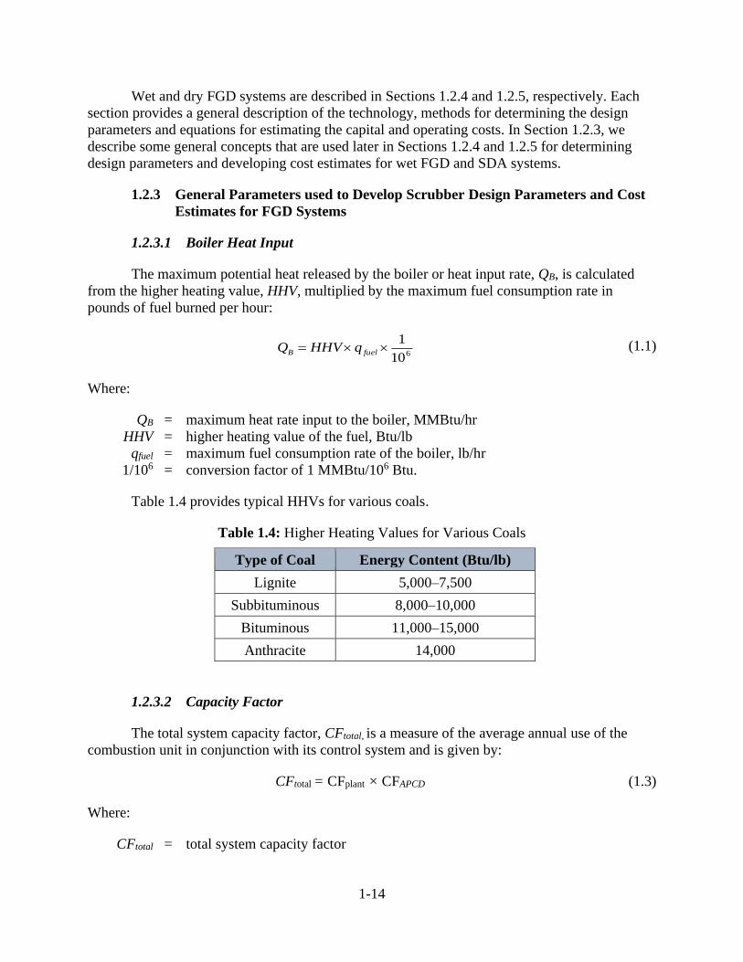
1.2.3.1 Boiler Heat Input
The maximum potential heat released by the boiler or heat input rate, QB, is calculated
from the higher heating value, HHV, multiplied by the maximum fuel consumption rate in
pounds of fuel burned per hour:
610
1= fuelB qHHVQ (1.1)
Where:
QB = maximum heat rate input to the boiler, MMBtu/hr
HHV = higher heating value of the fuel, Btu/lb
qfuel = maximum fuel consumption rate of the boiler, lb/hr
1/106 = conversion factor of 1 MMBtu/106 Btu.
Table 1.4 provides typical HHVs for various coals.
Table 1.4: Higher Heating Values for Various Coals
Type of Coal Energy Content (Btu/lb)
Lignite 5,000–7,500
Subbituminous 8,000–10,000
Bituminous 11,000–15,000
Anthracite 14,000
1.2.3.2 Capacity Factor
The total system capacity factor, CFtotal, is a measure of the average annual use of the
combustion unit in conjunction with its control system and is given by:
CFtotal = CFplant × CFAPCD (1.3)
Where:
CFtotal = total system capacity factor

1-15
CFplant = combustion unit capacity factor, which is the ratio of the actual quantity of fuel
burned annually to the potential maximum quantity of fuel burned
CFAPCD = air pollution control device capacity factor, which is the ratio of the actual days
the control device is operated to the total number of days the plant (or boiler)
operated during the year (tAPCD and tplant).
𝐶𝐹𝐴𝑃𝐶𝐷 =𝑡𝐴𝑃𝐶𝐷
𝑡𝑝𝑙𝑎𝑛𝑡 (1.4)
Where:
tAPCD = actual days the air pollution control device is operated annually, days/year
tplant = number of days the plant (or boiler) operated in a year, days.
The effective operating time per year, top, is estimated in hours using the system capacity
factor, CFtotal:
year
hoursCFt totalop 760,8= (1.5)
1.2.3.3 Heat Rate Factor
The heat rate factor (HRF) is the ratio of gross heat rate of the boiler in MMBtu/MWh
divided by 10 MMBtu/MWh. The cost methodology for the wet FGD presented in Section 1.2.3
and the SDA FGD presented in Section 1.2.4 use the HRF in the equations for the capital cost
estimates to account for observed differences in actual costs for different coal-fired combustion
units.
𝐻𝑅𝐹 =𝐻𝑅
10 (1.6)
Where:
HRF = Heat rate factor
HR = Gross plant heat rate of the system, MMBtu/MWh
10 = Heat rate basis of the SDA FGD and wet FGD base module capital costs, in
MMBtu/MWh.
1.2.3.4 Site Elevation Factor
The original cost calculations presented in Sections 1.2.3 and 1.2.4 for wet and dry FGD
systems were developed based on data for plants located within 500 feet of sea level. However,
for these two systems, the capital costs for the absorber (ABSCost) and the balance of plant costs
(BOPCost) are impacted by the plant site’s elevation with respect to sea level. Therefore, the base
cost equations for ABSCost and BOPCost are adjusted by elevation factor, ELEVF, for the effects of
elevation on the flue gas volumes encountered at elevations above 500 feet above sea level. The
elevation factor, ELEVF, is calculated using Equations 1.7 and 1.8 for plants located above 500

1-16
feet. For plants located at elevations below 500 feet elevation, an elevation factor of 1 should be
used to calculate the ABSCost and BOPCost [20, 21]
𝐸𝐿𝐸𝑉𝐹 = 𝑃0
𝑃𝐸𝐿𝐸𝑉 (1.7)
Where:
ELEVF = elevation factor
P0 = atmospheric pressure at sea level, 14.7 pounds per square inch absolute (psia)
PELEV = atmospheric pressure at elevation of the unit, psia.
The PELEV can be calculated using Equation 1.8 [22]:
𝑃𝐸𝐿𝐸𝑉 = 2116 × [59−(0.00356×ℎ)+459.7
518.6]
5.256
×1
144 (1.8)
Where:
PELEV = atmospheric pressure at elevation of the unit, psia
h = altitude, feet.
1.2.3.5 Retrofit Factor
Equipment and installation costs for FGD systems can vary significantly from site-to-site
depending on site characteristics. For this reason, the capital cost equations in Sections 1.2.4 for
wet FGD systems and 1.2.5 for SDA systems include a retrofit factor (RF) that allows users to
adjust the costs estimates, depending on the site-specific conditions and level of difficulty. An
RF of 1 should be used to estimate costs for a project of average difficulty. For retrofits that are
more complicated than average, a retrofit factor of greater than 1 can be used to estimate capital
costs provided the reasons for using a higher retrofit factor are appropriate and fully documented.
Similarly, new construction and retrofits of existing plants that are less complicated should use
an RF less than 1. Each project should be evaluated to determine the appropriate value for RF.
The capital costs for the control systems are calculated for multiple modules and then totaled.
The cost for each module is calculated using a separate equation with its own RF. Thus,
depending on the site-specific circumstances, different RFs may be used for different modules.
Factors that should be considered when evaluating the RF for retrofits include site
congestion, site access, and capacity of existing infrastructure. The amount of space available
near the utility boiler can significantly impact the costs. Site congestion can be caused by
existing generators, conveyors, and environmental control equipment. Costs will be higher if
portions of the FGD system must be elevated or existing generators, control equipment,
buildings, and other infrastructure must be relocated to accommodate the FGD system. In some
cases, site congestion results in the FGD system being installed further away from the boiler,
resulting in extra costs for additional duct work and fans. Costs can also be impacted if ancillary
equipment, such as wastewater treatment and absorbent storage and preparation areas, must be
located further from the absorber. A congested site can also increase construction costs by

1-17
requiring greater reliance on cranes to locate equipment and limiting access by construction
workers.
Site access can impact installation costs if it is difficult for cranes and other heavy
construction equipment to access the construction site. A retrofit for a plant that is bound on two
or more sides by adjacent generating units, roadways, rivers, wetlands, or other barriers will
likely be more challenging than sites that are more open for equipment access.
The capacity, condition, and location of existing infrastructure can also impact costs.
Costs will be lower if existing equipment can be used. For example, new fans may not be needed
where existing fans have adequate design margins for handling gas flow. If the site has an
existing FGD system, the existing ancillary units for absorbent storage and preparation
equipment may be sufficient to support the new system. Similarly, if two FGD systems are
planned to be installed at the same plant, costs may be reduced by installing a single wastewater
treatment system capable of treating FGD wastewater for both absorbers.
Based on the information available at the time this chapter was prepared, the RF value
should be between 0.7 and 1.3 for wet FGD systems and between 0.8 and 1.5 for dry FGD
systems, depending on the level of difficulty. Costs for new construction are typically, though
not for every instance, 20 to 30 percent less than for average retrofits for units of the same size
and design. An RF of 0.77 is recommended for estimating capital costs for new construction. [3,
52, 53]
1.2.4 Wet Flue Gas Desulfurization
1.2.4.1 Wet FGD Systems Process Description
The typical wet FGD system controls waste gases containing SO2 concentrations up to
2000 ppm using relatively inexpensive and readily available alkali reagents. A typical wet FGD
system consists of sorbent storage and preparation equipment, an absorber vessel, a mist
eliminator, and waste collection and treatment vessels. An additional or upgraded induced draft
fan may also be needed to compensate for the pressure drop across the absorber. Figure 1.2
shows a schematic of a wet FGD system using limestone as the sorbent. Most wet FGD systems
use a limestone sorbent that is prepared by first crushing the limestone into a fine powder using a
ball mill and then mixing the powder with water in the slurry preparation tank. Particle size of
the limestone impacts the efficiency of SO2 removal. In the typical wet limestone FGD system,
the limestone is ground to an average size of 5 to 20 μm. [15]
The sorbent slurry is pumped from the slurry preparation tank to the absorber. The flue
gas is ducted to the absorber where the aqueous slurry of sorbent is injected into the flue gas
stream through injection nozzles.

1-18
Figure 1.2: Flow Diagram for a Wet FGD System [14]
Although there are several different designs of absorbers, the most common is a counter-
flow, vertically oriented spray tower, where the flue gas flows upwards and the sorbent slurry is
sprayed downwards. The flue gas inlet temperature is typically between 300 and 700oF. The
design and location of the injection nozzles in the spray tower are selected to ensure the sorbent
is evenly dispersed in the flue gas stream and that contact between the flue gas and sorbent is
optimized. The flue gas becomes saturated with water vapor as a portion of the water in the
sorbent slurry is evaporated and the sorbent becomes fine droplets. SO2, and other acid gases
dissolve in the slurry and react with the sorbent to produce salts. The sorbent slurry falls to the
bottom of the absorber tower where it is collected and transferred to a waste handling system. [3,
14] A mist eliminator located immediately after the absorber removes any remaining slurry
droplets from the flue gas stream. The mist eliminator may be followed by a heat exchanger to
raise the temperature of the flue gas. The combined effect of the mist eliminator and heat
exchanger reduces opacity in the stack plume and reduces the potential for corrosion of
downstream equipment and ducts. [14] Due to the acidic properties of flue gas, corrosion is a
significant issue for FGD systems. Methods for mitigating corrosion are discussed in more detail
later in this section (see the section titled Potential Operating Issues for Wet FGD Systems-
Corrosion).
The waste from the absorber (called the slurry bleed) is collected, dewatered, and
transferred to an onsite or offsite disposal. Alternatively, the calcium sulfate may be recovered
and sold to wallboard manufacturers. Where calcium sulfate is recovered and sold to wallboard
manufacturers, the solids are typically dewatered with a vacuum belt and the liquid returned to
the FGD system as reclaimed water. [3, 14]

1-19
The wet FGD system may be a “regenerable” system where the sorbent is recovered from
the waste slurry and recycled back to the absorber, or “once-through” system where the waste
slurry is sent to a landfill for disposal or sold as byproduct. The majority of wet FGD systems are
once-through systems. [3, 23]
For systems using limestone, the overall reactions are summarized by the following
equations:
𝑆𝑂2 + 𝐶𝑎𝐶𝑂3 + 1/2𝐻2𝑂 → 𝐶𝑎𝑆𝑂3 ∙ 1/2𝐻2𝑂 + 𝐶𝑂2
𝑆𝑂2 + 1/2𝑂2 + 𝐶𝑎𝐶𝑂3 + 2𝐻2𝑂 → 𝐶𝑎𝑆𝑂4 ∙ 2𝐻2𝑂 + 𝐶𝑂2
The calcium carbonate (CaCO3) in limestone is only slightly soluble in water, but in the
presence of acid, it reacts much more vigorously. It is the acid generated by absorption of the
SO2 into the liquid that drives the limestone dissolution process. [24]
The degree to which the calcium sulfite is converted to calcium sulfate depends on the
amount of oxygen present in the absorber and reaction vessel. High levels of oxygen result in
higher yields of calcium sulfate (gypsum), which can be sold as a byproduct. [14] For example,
gypsum can be sold to cement plants or wallboard manufacturers. [9] The slurry is filtered to
recover the gypsum. The gypsum is then dewatered before shipping offsite. The water from
filtration is typically sent to a wastewater treatment plant or recirculated back into the FGD
system. The typical wastewater treatment consists of increasing the pH to precipitate metals as
metal hydroxides. Additives may be added to promote coagulation and flocculation. [15]
In addition to the basic system described above, there are four design variations on the
wet FGD system:
1. Limestone Slurry Forced Oxidation (LSFO):
Conventional wet limestone FGDs operate under natural oxidation where CaSO3 is only
partly oxidized by the oxygen contained in the flue gas. The product produced is a 50% to 60%
mixture of CaSO3∙1/2H2O and CaSO4∙2H2O, which is a soft, difficult-to-dewater material that
has little practical value.
Many existing scrubbers are equipped with forced-air oxidation systems in which air is
injected in the reaction tank and the oxygen converts Ca (HSO3)2 to CaSO4. The result is a
product that contains 90% CaSO4∙2H2O. Dewatering of the filtered product is also easier
because the gypsum crystals are larger (<100 micrometers or microns, μm) than those produced
by natural oxidation in a conventional wet limestone FGD system (<5 μm). [14, 15] Seed
crystals of calcium sulfate are used to promote rapid precipitation of the calcium sulfate, which is
then dewatered. The air can be blown into either the reaction tank or into an additional holding
tank. [14] Sulfate precipitates with calcium as gypsum, which typically forms a cake-like
material when subjected to vacuum filtration.
Capital costs are higher than those for the basic wet FGD system as additional
compressors, blowers, and piping are required. [14] However, modern scrubber systems can

1-20
produce gypsum “cake” with as little as 10% moisture (water content by mass), which makes it
very easy to handle or sell to wallboard manufacturers.[24] For example, in 2018, the Centralia
power plant reported 0.04 – 0.05 lb/mmBtu annual SO2 emissions from its tangentially-fired
boilers and all gypsum produced by the scrubber is recycled in the production of wallboard.
2. Limestone Inhibited Oxidation (LSIO):
Sulfur or sodium thiosulfate is added to the limestone slurry to inhibit the oxidation of
calcium sulfite to calcium sulfate (gypsum). LSIO systems can be used to control waste gas with
higher SO2 concentrations than systems using only limestone. The waste CaSO3 produced by the
LSIO system must be landfilled. [3, 14]
3. Lime Process:
This process uses calcium hydroxide (lime slurry) instead of the limestone slurry in a
countercurrent spray tower. The hydrated lime reacts more readily with the dissolved SO2 than
does the limestone slurry. Hence, less lime is needed to achieve the same level of SO2 removal.
However, the lime process is generally more expensive to operate than a limestone-based system
due to the higher cost of the lime. The lime process can also use fly ash to increase the alkalinity
of the sorbent slurry. [3, 14]
For systems using lime, the overall reactions are summarized by the following equations:
𝐶𝑎𝑂 + 𝐻2𝑂 → 𝐶𝑎(𝑂𝐻)2𝑆𝑂2 + 𝐻2𝑂 ⇆ 𝐻2𝑆𝑂3
𝐻2𝑆𝑂3 + 𝐶𝑎(𝑂𝐻)2 → 𝐶𝑎𝑆𝑂3 + 2𝐻2𝑂
𝐶𝑎𝑆𝑂3 + 1/2𝑂2 → 𝐶𝑎𝑆𝑂4
4. Magnesium Enhanced-Lime Process (MEL):
MEL uses either magnesium-enhanced lime that contains approximately 5% to 8%
magnesium oxide (MgO) or dolomite lime that contains about 20% magnesium oxide. MEL
achieves higher SO2 removal efficiencies and uses less sorbent. The MgO in the lime reacts with
SO2 to form soluble magnesium sulfite (MgSO3). The MgSO3 accumulates in the lime slurry and
acts as a pH buffer, which increases the mass transfer of SO2 resulting in SO2 removal of greater
than 95% at low liquid-to-gas ratio. For example, one system achieved 96% SO2 removal with an
L/G ratio of 21 gpm per 1000 acfm. [25]
For systems using MEL, the overall reactions for magnesium oxide are summarized by
the following equations:
𝑀𝑔𝑂 + 𝑆𝑂3 → 𝑀𝑔𝑆𝑂4
𝑀𝑔𝑂 + 𝑆𝑂2 → 𝑀𝑔𝑆𝑂3
𝑀𝑔𝑆𝑂3 + 1/2𝑂2 → 𝑀𝑔𝑆𝑂4

1-21
The magnesium sulfite formed in the absorber is water soluble and therefore less likely to
form deposits inside the absorber and on downstream ductwork. Forced oxidation downstream
from the absorber can be used to convert MgSO3 and CaSO3 to MgSO4 and CaSO4∙2H2O
(gypsum). The gypsum is recovered by filtration and sold to either cement or wallboard
manufacturers. Most of the filtrate is returned to the absorber. However, some of the filtrate is
removed to purge accumulated salts, including MgSO4 and MgCl2, which can be used to produce
magnesium hydroxide (Mg(OH)2). [14, 25]
Factors Affecting Wet FGD System Operation
The principal factors affecting the operation of a wet FGD system are:
1. Flue gas flow rate;
2. Liquid-to-gas (L/G) ratio;
3. Flue gas SO2 concentration;
4. Distribution of the flue gas and sorbent in the absorber;
5. Oxygen level in the absorber and reaction tank;
6. Slurry pH;
7. Slurry solids concentration; and
8. Solids retention time.
Flue Gas Flow Rate. The optimal waste gas flow rate for a wet FGD system is dependent
on the design of the absorber unit. For some absorbers, such as those using the counterflow
design, the maximum waste gas flow rate is dependent on the capacity of the mist eliminator. For
absorbers that use trays, the waste gas flow rate is limited to a specific range to prevent flooding
of the scrubber. [26]
Liquid-to-gas (L/G) ratio. The liquid-to-gas (L/G) ratio (in gallons of slurry per 1000 ft3
of flue gas) in the wet FGD system is optimized to achieve the highest absorption and reaction
rate, and hence the highest SO2 removal. Systems that use higher amounts of sorbent (i.e., have
higher L/G ratios) can achieve higher removal efficiencies. However, increasing the L/G ratio
results in higher sorbent consumption and higher operating costs. The L/G ratio for wet FGD
systems using limestone as sorbent is typically 40-100 gal to 1000 cfm. [14]
Flue Gas SO2 Concentration. In general, the SO2 removal efficiency decreases as the SO2
concentration in the inlet waste gas stream increases. The high SO2 concentrations result in rapid
reductions in the alkalinity of the sorbent liquid and reduce the amount of SO2 that will be
dissolved in the liquid slurry droplets, which reduces the amount of SO2 reacting with the
sorbent. [14] SO2 removal efficiency is also lower when the SO2 concentration in the inlet waste
gas stream is very low.
Distribution of the flue gas and sorbent in the absorber. Good distribution of the flue gas
and sorbent within the absorber is necessary to ensure maximum SO2 removal. Poor distribution
of sorbent and flue gas can be compensated for by increasing the L/G ratio, however, this results
in higher operating costs due to the increased sorbent usage. Wet FGDs use spray nozzles that
atomize the sorbent to maximize the contact between the sorbent and the flue gas. Other
techniques, such as installing guide vanes along the perimeter of the tower, may be used to
improve mixing.[14]

1-22
Oxygen Level. The level of oxygen available in the absorber and reaction tank affects the
chemical balance between CaSO3 and CaSO4. Oxidizing conditions in the absorber and reaction
vessel favor the production of CaSO4 since CaSO3 is converted to CaSO4. Since CaSO4 is easier
to dewater, many wet FGD systems use limestone slurry forced oxidation (LSFO) systems. In
these systems, air is injected into the reaction tank, which oxidizes the calcium sulfite to calcium
sulfate (gypsum). The gypsum crystals formed by the LSFO are larger and settle out from the
wastewater more readily and makes the processing of the FGD system waste easier and less
expensive. However, the LSFO system requires air blowers that increase the capital and
operating costs for LSFO equipped wet FGD systems. [14]
Slurry pH. In the reaction tank the dissolution and crystallization reactions are controlled
by the pH of the liquid, which is a function of limestone stoichiometry. The pH and limestone
stoichiometry are preset parameters that are monitored and used to control the operation of the
absorber. The stoichiometry for a wet FGD system using limestone as the sorbent typically
varies from 1.01 to 1.1 moles of CaCO3 per mole of SO2. The pH is typically maintained between
5.0 to 6.0. The pH is used to determine the amount of limestone added to the absorber. A drop in
the pH of the reaction vessel, for example, indicates increased SO2 in the flue gas, increased
consumption of the sorbent, and triggers an increase in the feed rate of the sorbent. [14]
Slurry Solids Concentration. In addition to the pH, the solids concentration in the slurry
is also important for the correct operation of the wet FGD system because high solids content can
cause scaling to occur in the absorber (discussed below). The solids concentration of the slurry is
monitored. The typical system maintains the slurry solids concentration between 10% and 15%
by weight. [14]
Solids Retention Time. The retention time for solids in the reaction tank is important for
achieving high utilization of the sorbent. It also ensures the dewatering properties of solids is
managed correctly. For a typical wet FGD system, the solids retention time is 12 to 14 hours.
[14]
Types of Sorbent
Wet FGD systems use limestone (CaCO3) or lime (Ca(OH)2) as the sorbent. Limestone is
the most commonly used sorbent because of its low cost. Typical wet FGD systems using lime or
limestone as the sorbent can achieve SO2 removal efficiencies of between 95% and 99%.
However, the removal efficiency for limestone-based systems can be lower than those using
lime. Lime is more reactive and easier to handle than limestone. Some researchers have found
that aluminum and silicon impurities in limestone are retained in recovered gypsum product.
Limestone with purity above 95% is recommended for wet limestone FGDs. [3, 14, 15] Typical
costs for limestone and lime are reported to be $28/ton and $75/ton, respectively, based on 2016
data. [27]
Some manufacturers sell proprietary sorbents that contain additives (e.g., dibasic acid
(DBA), formic acid) designed to promote the absorption and reaction of SO2. These additives
buffer the scrubber slurry, which controls the SO2 vapor pressure in the scrubber and thereby
maximizes the SO2 adsorption rate. Wet FGD systems using these proprietary sorbents can
achieve SO2 removal efficiencies of 97% to 99%. [3, 18, 27]
1-23
Wet FGD systems that use seawater as the sorbent solution are also available. In these
systems, the limestone dissolves completely in the seawater. The SO2 reacts with the sorbent
liquid in a counterflow absorber. The sulfate produced remains in solution in the seawater and is
discharged into the ocean. Generally, wastewater treatment is not required as sulfate salts are
already present in seawater and the increase in concentration is minimal. However, the high
chloride concentration of seawater can result in corrosion problems. Hence, wet FGD systems
using seawater must be constructed of corrosion resistant materials that increase the capital costs.
[14]
Removal Efficiency
Wet FGD systems typically achieve between 90% and 99% removal efficiency. The
typical LSFO system can achieve 96% SO2 removal efficiency and SO2 emission rates as low as
0.06 lbs/MMBtu. [3, 10] In 2018, the Centralia power plant reported 0.04 – 0.05 lb/mmBtu
annual SO2 emissions from its tangentially-fired boilers with LSFO.
Factors impacting the removal efficiency include the type and quantity of sorbent used,
effectiveness of the sorbent injection system in dispersing the sorbent slurry throughout the flue
gas stream and the concentration of SO2 in the flue gas. Removal efficiencies are also impacted
by the amount of sorbent used. The liquid-to-gas (L/G) ratio (in gallons of slurry per 1000 ft3 of
flue gas) is typically used to provide a guide to optimizing the design of a wet scrubber system.
Systems that use higher amounts of sorbent (i.e., have higher L/G ratios) can achieve higher
removal efficiencies. [14]
Wastewater Treatment
Wet FGD scrubber systems may be either recirculating or once-through wet FGD
systems. In a recirculating system, most of the slurry at the bottom of the scrubber is recirculated
back within the scrubber and occasionally a blowdown or bleed stream is transferred to a solids
separator, where the wastewater is either recycled back to the scrubber or transferred to a
wastewater treatment system. In a once-through system, all of the FGD slurry at the bottom of
the scrubber is transferred to the solids separator without being recirculated. In addition to the
wastewater generated by the solids separator, wastewater may also be generated from the solids
drying process and from gypsum washing. [57, 58, 59]
Wastewater generated by wet FGD systems often contain metals, such as arsenic,
beryllium, cadmium, chromium, mercury, lead, selenium, and copper, as well as other pollutants,
including cyanide, ammonia, phosphorus, nitrogen, and total suspended solids (TSS). Pollutant
concentrations vary depending on numerous factors, including the type of fuel burned, type of
sorbent used, the level of recirculation of the slurry before discharge, and the materials used in
the construction of the wet FGD system. The types of air pollution controls operated upstream of
the wet FGD system can also affect the wastewater characteristics. For example, plants that
operate a particulate collection system (e.g., electrostatic precipitator) upstream from the wet
FGD system will generate wastewater with lower levels of arsenic, mercury, and TSS due to the
removal of fly ash. [57, 58]

1-24
The EPA published technology-based effluent limitations guidelines and standards
(ELGs) for the steam electric power generating point source category in 2015, which included
ELGs for wastewater generated by wet FGD systems. The rule set standards for both the direct
discharge of FGD wastewater to surface water and the discharge to a publicly owned treatment
works (POTW). The rule included ELGs for both new sources (greenfield) and existing sources.
The EPA revised the 2015 ELGs for FGD wastewater at existing plants in 2020. As a result,
wastewater generated by wet FGD systems are subject to numeric effluent limitations on
mercury, arsenic, selenium, and nitrate/nitrite such as nitrogen. [57]
For existing facilities, the ELGs can be met using chemical precipitation followed by
biological treatment and filtration as a final polishing step. For the chemical precipitation
pretreatment step, chemicals are added to help remove suspended and dissolved solids and
metals. The precipitated solids are then removed from solution by coagulation/flocculation,
followed by clarification and/or filtration. The chemical precipitation uses hydroxide
precipitation, sulfide precipitation (organosulfide), and iron coprecipitation to remove suspended
solids and to convert soluble metal ions to insoluble metal hydroxides or sulfides. [57]
In the biological treatment step, microorganisms are used to treat the FGD wastewater.
The 2015 rule focused on a high residence time biological reduction system that uses
anoxic/anaerobic fixed-film bioreactors with a residence time of approximately 10 to 16 hours.
For the 2020 amendments, EPA based in the revised ELGs for existing plants on low hydraulic
residence time biological reduction (LRTR), which is a biological treatment system that targets
removal of selenium and nitrate/nitrite using fixed-film bioreactors in smaller, more compact
reaction vessels than those used in the biological treatment system evaluated in the 2015 rule
(i.e., high residence time biological reduction). The LRTR system is designed to operate with a
shorter residence time (approximately 1 to 4 hours), while still removing significant volumes of
selenium and nitrate/nitrite. [57]
For new plants, the ELGs were based on a thermal evaporation process that uses a
falling-film evaporator or brine concentrator to produce a concentrated wastewater stream and a
distillate stream. The thermal evaporation process reduces the volume of wastewater by 80 to
90% thereby reducing the discharge of pollutants. The concentrated wastewater is usually further
processed in a crystallizer, which produces a solid residue for landfill disposal and additional
distillate that can be reused within the plant or discharged. The principal benefit of using a
thermal evaporation process is that it removes a broad range of pollutants.
The ELG includes a Voluntary Incentives Program that allows existing plants until
December 31, 2028 to comply if they adopt additional process changes and controls that achieve
more stringent limitations on mercury, arsenic, selenium, nitrate/nitrite, bromide, and TDS. [57]
Potential Operating Issues for Wet FGD Systems
Corrosion. Both the acids in the flue gas and the sorbent slurry can cause significant
corrosion in wet FGD systems. Acids are formed when the hot, dry flue gases initially enter the
moist environment of the absorber vessel. The sorbent slurry is abrasive and can cause pitting of
metal surfaces that increases the risk of corrosion. Flue gas exiting the absorber is saturated with
1-25
water that contains some acidic gases (e.g., SO3) that are corrosive to downstream equipment
such as fans, ducts, and stacks. The high temperatures and presence of halides in the flue gas
(primarily chlorides and fluorides from impurities in limestone and coal) also contribute to the
corrosive conditions.[14, 28]
For constructing the absorbers and ancillary equipment (e.g., slurry tanks, pumps,
downstream control system components and stacks), manufacturers select materials that can
withstand the corrosive conditions that prevail in each component of the FGD system. The level
of acidity within the various components can vary significantly. For example, the pH of gas
entering the absorber can be as low as 1, while the acidity in the absorber typically ranges from
to 4.0 to 5.5. The flue gas leaving the absorber contains some acid, which will condense if the
gas contacts cold duct walls as it exits through the outlet ducting and chimney stack. The
condensate is highly acidic and can cause significant corrosion. The flue gas leaving the stack
can mix with moisture in the atmosphere, forming acidic droplets that fall into the stack and
cause corrosion to occur on the stack walls. [28] The cost for retrofitting an existing stack with
corrosion-resistant liners can be sufficiently high that, for some retrofits, the cost of retrofitting
an existing stack can be higher than the cost of replacing the existing stack with a new stack. [52]
Nickel alloys and nickel-alloy clad steel can be used to construct components that
experience the most corrosive conditions. Nickel alloys are often used to fabricate the absorber
outlet duct, any downstream auxiliary equipment (e.g., wet electrostatic precipitator, heat
exchanger) and chimney stack. Nickel-chromium and iron-nickel chromium alloys that contain
molybdenum have been found to be effective in FGD systems, with alloys containing more
molybdenum found to be the most resistant to corrosion. Super-austenitic stainless steels
containing 6% to 7% molybdenum can be used for fabricating the absorber vessel, while
austenitic stainless steels and duplex alloys can be used to fabricate components of the FGD
system that experience less corrosive environments (e.g., the inlet and bypass ducts). [28] Using
high alloy containing steels or rubber-lined absorber vessels or pumps increases the reliability of
the wet FGD system but can increase the capital cost by 10-20%. [52]
Fiberglass reinforced plastics (FRP) have also been used in FGD systems as a reliable
and less expensive alternative to nickel alloys. Chemical resistance of FRP made from epoxy
vinyl ester resin is said to be equivalent to nickel alloys. FRP are not chemically affected by the
majority of chloride and sulfite trace elements found in FGD systems that increase the
susceptibility of stainless steel to pitting and stress-corrosion cracking. Although some FRP are
reported to withstand temperatures of up to 600 oF, FRP are generally used in applications of
between 300 to 400oF. However, FRP may not be suitable for systems where temperatures
exceed 600°F for more than a few minutes, where wide swings in temperature occur, or where
extreme abrasive conditions exist. [54, 55]
To reduce corrosion inside the absorber, some absorbers use spray systems that
continuously wash the inside walls with slurry. The absorber vessel floor and ducts are designed
so that condensate is drained from the system. Chimney stacks are typically constructed of nickel
alloy clad steel and have condensate collection systems made of alloy plate to collect condensate
that forms on the interior walls of the stack. [28]

1-26
To minimize corrosion problems in equipment downstream from the absorber, many
manufacturers also use mist eliminators followed by heat exchangers. The mist eliminator
removes any remaining droplets of slurry from the flue gas stream. The heat exchangers keep the
temperature of the exhaust gases above their dew point and reduce condensation inside the ducts,
fans and stack. This approach also reduces plume opacity. [14, 28] Electrochemical protection
has been demonstrated to reduce corrosion in reaction tanks. [29]
Scale Formation. Calcium sulfate (gypsum) formed from the oxidation of calcium sulfite
can form scale in the absorber, mist collector and downstream ducts. Scale formation generally
occurs when the fraction of calcium sulfate in the slurry exceeds 15 percent. Scale formation can
be reduced by increasing the L/G ratio, using LSFO technology described above, or by using the
limestone inhibition oxidation process (LSIO). In the LSIO process, sulfur or sodium thiosulfate
(Na2S2O3) is added to the limestone slurry to prevent oxidation of the sulfite to sulfate. Where
sulfur is used in place of Na2S2O3, between 50% and 75% of the sulfur reacts with sulfite to
produce thiosulfate. The amount of Na2S2O3 added depends on the SO2 emissions and the
amount of oxygen in the waste gas stream. LSIO is useful for applications where coal with high
sulfur content is burned. [14]
High levels of chlorine in the flue gas can also contribute to scale formation as the
chlorine reacts with the sorbent to produce calcium chloride. [14, 26]
1.2.4.2 Wet FGD System Design Procedures
Methods for estimating the limestone feed rate, make-up water consumption, waste
generation rate and auxiliary power consumption for a wet FGD system are presented in this
section. These parameters are used in the cost methodology presented in Section 1.2.3.4 for
estimating the annual costs for operating a wet FGD system. The methods presented in this
section are those developed by the EPA’s Clean Air Markets Division (CAMD) for the
Integrated Planning Model (IPM) and its cost methodology. [21]
Limestone Feed Rate
Reagent usage is a function of the combustion unit size, SO2 emission rate and the
removal efficiency of the wet FGD system. In the IPM, the reagent feed rate equation is based on
a 98% SO2 removal. The equation below includes an adjustment factor that allows the reagent
usage to be adjusted to reflect the actual or target removal efficiency. The IPM cost methodology
also assumes a calcium-to-sulfur stoichiometric ratio of 1.03 and a limestone purity of 90%
CaCO3, with the balance being inert materials. The reagent usage rate is calculated as follows:
𝑄𝐿𝑖𝑚𝑒𝑠𝑡𝑜𝑛𝑒 =17.52×𝐴×𝑆×𝐻𝑅𝐹
2,000×
𝐸𝐹
0.98 (1.9)
Where
QLimestone = lime consumption rate, tons/hour
S = uncontrolled SO2 emission rate, lb/MMBtu
A = Unit size (Gross), MW
HRF = heat rate factor (calculated using Equation 1.6)

1-27
EF = removal efficiency, fraction
0.98 = SO2 removal efficiency basis (listed as a fraction) for the IPM cost model.
Make-up Water
The makeup water rate is a function of combustion unit size and SO2 emissions. The
make-up water consumption rate for a wet FGD system is calculated using the following
equation:
𝑞𝑤𝑎𝑡𝑒𝑟 =[(1.674×𝑆)+74.68]×𝐴×𝐶𝑜𝑎𝑙𝐹×𝐻𝑅𝐹
1,000 (1.10)
Where
qwater = make-up water consumption rate, 1,000 gallons (kgallons)/hour
S = uncontrolled SO2 emission rate, lb/MMBtu
A = Unit size (Gross), MW
CoalF = coal factor (CoalF=1 if bituminous; CoalF=1.05 if Powder River Basin (PRB)2;
CoalF=1.07 if Lignite)
HRF = heat rate factor (calculated using Equation 1.6).
Waste Generation Rate
The waste generation rate is directly proportional to the reagent usage. The wastewater
generation rate estimation method in the IPM assumes a 10% moisture content in the by-product
and is based on an SO2 removal of 98% of the inlet SO2. The ratio of the actual removal
efficiency to the base model removal efficiency of 98% adjusts the waste generation rate for
actual or target removal efficiency of the wet FGD system.
𝑞𝑤𝑎𝑠𝑡𝑒 = 1.811 × 𝑄𝐿𝑖𝑚𝑒𝑠𝑡𝑜𝑛𝑒 ×𝐸𝐹
0.98 (1.11)
Where:
qwaste = waste generation rate, tons/hour
QLimestone = limestone input rate, tons/hour
EF = SO2 removal efficiency, fraction
0.98 = SO2 removal efficiency basis for the IPM cost methodology.
Auxiliary Power Costs
The auxiliary power (also commonly called parasitic energy loss) is the additional power
required to operate the wet FGD system. The additional auxiliary power required for the wet
FGD system in kilowatts (kW) is estimated in the IPM as a percentage of the total unit gross
production and is dependent on the sulfur emissions and size of the combustion unit. The
2PRB was the most common type of subbituminous coal in use in the U.S. as of 2016. Also, PRB was approximately
95% of all subbituminous coal produced in the U.S., based on coal production data from the Energy Information
Administration’s (EIA) December 2019 Quarterly Coal Report (Table 2) and the 2018 Annual Coal Report (Table
ES1).
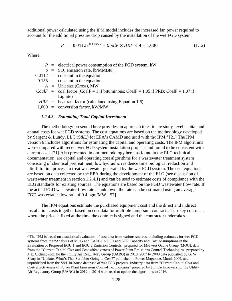
1-28
additional power calculated using the IPM model includes the increased fan power required to
account for the additional pressure drop caused by the installation of the wet FGD system.
𝑃 = 0.0112𝑒0.155×𝑆 × 𝐶𝑜𝑎𝑙𝐹 × 𝐻𝑅𝐹 × 𝐴 × 1,000 (1.12)
Where:
P = electrical power consumption of the FGD system, kW
S = SO2 emission rate, lb/MMBtu
0.0112 = constant in the equation
0.155 = constant in the equation
A = Unit size (Gross), MW
CoalF = coal factor (CoalF = 1 if bituminous; CoalF = 1.05 if PRB; CoalF = 1.07 if
Lignite)
HRF = heat rate factor (calculated using Equation 1.6)
1,000 = conversion factor, kW/MW.
1.2.4.3 Estimating Total Capital Investment
The methodology presented here provides an approach to estimate study-level capital and
annual costs for wet FGD systems. The cost equations are based on the methodology developed
by Sargent & Lundy, LLC (S&L) for EPA’s CAMD and used with the IPM.3 [21] The IPM
version 6 includes algorithms for estimating the capital and operating costs. The IPM algorithms
were compared with recent wet FGD system installation projects and found to be consistent with
current costs.[21] Also presented in our methodology here, as found in the ELG technical
documentation, are capital and operating cost algorithms for a wastewater treatment system
consisting of chemical pretreatment, low hydraulic residence time biological reduction and
ultrafiltration process to treat wastewater generated by the wet FGD system. The cost equations
are based on data collected by the EPA during the development of the ELG (see discussion of
wastewater treatment in section 1.2.4.1) and can be used to estimate costs of compliance with the
ELG standards for existing sources. The equations are based on the FGD wastewater flow rate. If
the actual FGD wastewater flow rate is unknown, the rate can be estimated using an average
FGD wastewater flow rate of 0.4 pgm/MW. [57]
The IPM equations estimate the purchased equipment cost and the direct and indirect
installation costs together based on cost data for multiple lump-sum contracts. Turnkey contracts,
where the price is fixed at the time the contract is signed and the contractor undertakes
3 The IPM is based on a statistical evaluation of cost data from various sources, including estimates for wet FGD
systems from the “Analysis of MOG and LADCO's FGD and SCR Capacity and Cost Assumptions in the
Evaluation of Proposed EGU 1 and EGU 2 Emission Controls” prepared for Midwest Ozone Group (MOG), data
from the “Current Capital Cost and Cost-effectiveness of Power Plant Emissions Control Technologies” prepared by
J. E. Cichanowicz for the Utility Air Regulatory Group (UARG) in 2010, 2007 to 2008 data published by G. W.
Sharp in “Update: What’s That Scrubber Going to Cost?” published in Power Magazine, March 2009, and
unpublished from the S&L in-house database of wet FGD projects. Industry data from “Current Capital Cost and
Cost-effectiveness of Power Plant Emissions Control Technologies” prepared by J.E. Cichanowicz for the Utility
Air Regulatory Group (UARG) in 2012 to 2014 were used to update the algorithms to 2016.

1-29
responsibility for the completion of the project, are generally 10 to 15% higher than the multiple
lump-sum contracts. The capital costs equations estimate costs in 2016 dollars.
The capital costs estimated using the IPM methodology are consistent with the installed
costs reported to the U.S. Department of Energy, Energy Information Administration (EIA). The
EIA data includes various designs of wet FGD systems. For those systems with removal
efficiency of 90% or greater, the installed costs reported to EIA range between $250,000 to $709
million, with an average cost of $114 million. For a 500 MW unit calculated using the IPM
methodology, the TCI is estimated at $244 million (see the example in Section 1.2.3.6).
The capital cost equations developed by S&L are for typical wet FGD system
installations retrofitted on existing coal-fired utility units of capacity of over 100 MW (or 1,000
MMBtu/hour), achieving a removal efficiency of 98% with SO2 emission level of 0.06lb/MMBtu
Over 100 MW (or 1,000 MMBtu/hour). For units under 100 MW, capital costs for a wet FGD
system are approximately $900/kW. [21]
The capital costs for units over 100 MW are impacted primarily by the unit size and the
type and sulfur content of the coal burned. The larger the size of the combustion unit, the larger
the amount of flue gas generated. The size of the absorber, reagent preparation equipment, waste
handling, and the balance of plant costs are all impacted by the quantity of flue gas generated.
The size and cost of the reagent and waste handling equipment are also dependent on the type of
coal burned. The capital cost estimated using this methodology includes the capital costs for a
wastewater treatment facility consisting of only minor physical and chemical wastewater
treatment. The capital costs should be adjusted if a more extensive wastewater treatment system
is required at a specific plant site.
Total capital investment (TCI) includes direct and indirect costs associated with
purchasing and installing the wet FGD system equipment. TCI includes the equipment cost for
the wet FGD system, the cost of auxiliary equipment, direct and indirect installation costs,
additional costs due to installation, costs for buildings and site preparation, cost of land and
working capital. A more detailed discussion of what is included in capital costs can be found in
Section 1, Chapter 2 of this Manual.
Cost calculations in the IPM are based primarily on data for retrofits. However, retrofits
are typically 30% more than for new units of the same size and design. [3] To adjust for the
additional costs associated with retrofits, we have included a retrofit factor in the TCI equations.
A retrofit factor of 0.77 should be used to estimate capital costs for new construction using these
equations and a retrofit factor of 1 should be used for wet FGD system retrofits to existing units,
where the retrofit is of an average level of difficulty. Retrofit costs vary significantly from site to
site and depend on the amount of space available and whether significant modifications to
existing equipment (e.g., ductwork, stack) are needed. A higher retrofit factor should be used for
congested sites.
The IPM capital cost equation for a wet FGD system is presented in Equation 1.13:
𝑇𝐶𝐼 = 1.3 × (𝐴𝐵𝑆𝐶𝑜𝑠𝑡 + 𝑅𝑃𝐸𝐶𝑜𝑠𝑡 + 𝑊𝐻𝐸𝑐𝑜𝑠 𝑡 + 𝐵𝑂𝑃𝐶𝑜𝑠𝑡) + 𝑊𝑊𝑇𝐶𝑜𝑠𝑡 (1.13)

1-30
Where:
TCI = total capital investment for a wet FGD system, $
ABSCost = cost of the absorber island, $
RPECost = reagent preparation equipment cost, $
WHECost = waste handling equipment cost, $
BOPCost = balance of plant costs, $
WWTCost = cost of wastewater treatment facilities, $.
The TCI calculation shown in Equation 1.13 includes a factor of 1.3 to estimate
engineering and construction management costs, installation, labor adjustment for the wet FGD
system, and contractor profit and fees. The owner’s costs (for owner activities related to
engineering, management, and procurement) and costs such as allowance for funds used during
construction (AFUDC) are capital cost items that are not included in the EPA Control Cost
Manual methodology and are inconsistent with the overnight cost method4 that is a key basis for
the Control Cost Manual methodology, and thus are not included in the TCI estimates in this
section or in other Control Cost Manual chapters. The 1.3 factor does not apply to the wastewater
treatment system as the direct and indirect costs for the wastewater system are included in the
cost equations.
The costs for the absorber island (ABSCost), reagent preparation (RPECost), waste handling
equipment (WHEcost), balance of plant costs (BOPCost) and wastewater treatment facility
(WWTCost) are discussed in the following sections. The estimated cost varies depending on the
size (or capacity) of the unit. The gross heat rate impacts the amount of flue gas generated and
ultimately impacts the size of the absorber, reagent preparation, waste handling, and the balance
of plant costs. The SO2 emissions rate primarily impacts the capital costs of the reagent and
waste handling facilities, while the type of fuel burned impacts the quantity of flue gas and
thereby impacts the BOPCost.
The ABSCost and BOPCost are also impacted by the unit’s elevation with respect to sea
level. The original cost calculations were developed for wet FGD systems located within 500
feet of sea level. Therefore, for plants located at higher elevations, the base costs should be
adjusted for the effects of elevation on the flue gas volume using an elevation factor, ELEVF.
The elevation factor, ELEVF, is 1 for plants located below 500 feet above sea level. If the plant
is located more than 500 feet above sea level, ELEVF is calculated using Equations 1.7 and 1.8
in Section 1.2.2.4.
The capital costs for the absorber island are estimated as follows:
𝐴𝐵𝑆𝐶𝑜𝑠𝑡 = 584,000 × 𝑅𝐹 × (𝐶𝑜𝑎𝑙𝐹 × 𝐻𝑅𝐹)0.6 × (𝑆/2)0.02 × 𝐴0.716 × 𝐸𝐿𝐸𝑉𝐹 (1.14)
4 The overnight cost estimation method presumes costs are incurred as if the project in question incurred no interest
during construction, or was built “overnight.” Another description of this method is the present value cost that would
have to be paid as a lump sum up front to completely pay for a construction project. For more information, see
“Conducting Technical and Economic Evaluations – As Applied for the Process and Utility Industries,”
Recommended Practice 16R-90, American Association of Cost Engineering International. April 1991, and Section
1, Chapter 2 of this Control Cost Manual.

1-31
Where
ABSCost = Wet FGD system absorber island costs, $
584,000 = constant
HRF = heat rate factor
CoalF = coal factor (CoalF = 1 if bituminous; CoalF = 1.05 if PRB; CoalF = 1.07 if
Lignite)
S = SO2 emission rate, lb/MMBtu
RF = retrofit factor (RF = 0.77 for new construction; RF = 1 for retrofits with average
level of difficulty)
A = Unit size (Gross), MW
ELEVF = elevation factor (calculated using Equations 1.7 and 1.8, if plant is located
above 500 feet above sea level; ELEVF = 1 for plants located at 500 ft above
sea level).
The reagent preparation and handling equipment costs (RPECost) for wet FGD systems are
calculated as follows:
𝑅𝑃𝐸𝐶𝑜𝑠𝑡 = 202,000 × 𝑅𝐹 × (𝑆 × 𝐻𝑅𝐹)0.3 × 𝐴0.716 (1.15)
Where:
RPECost = reagent preparation and handling equipment cost, $
202,000 = constant in the equation
S = SO2 emission rate, lb/MMBtu
RF = retrofit factor (RF = 0.77 for new construction; RF = 1 for retrofits with
average level of difficulty)
HRF = heat rate factor (calculated using Equation 1.6)
A = Unit size (Gross), MW.
The waste handling equipment costs (WHEcost) are calculated as follows:
𝑊𝐻𝐸𝐶𝑜𝑠𝑡 = 106,000 × 𝑅𝐹 × (𝑆 × 𝐻𝑅𝐹)0.45 × 𝐴0.716 (1.16)
Where:
WHECost = Waste handling equipment costs, $
106,000 = constant in the equation
A = Unit size (Gross), MW
HRF = heat rate factor
S = SO2 emission rate, lb/MMBtu
RF = retrofit factor (RF = 0.77 for new construction; RF = 1 for retrofits with
average level of difficulty).
The BOPCost are calculated as follows:
𝐵𝑂𝑃𝐶𝑜𝑠𝑡 = 1,070,000 × 𝑅𝐹 × (𝐶𝑜𝑎𝑙𝐹 × 𝐻𝑅𝐹)0.4 × 𝐴0.716 × 𝐸𝐿𝐸𝑉𝐹 (1.17)

1-32
Where:
BOPCost = Balance of plant costs, $
1,070,000 = constant in the equation
A = Unit size (Gross), MW
HRF = heat rate factor
CoalF = coal factor (CoalF = 1 if bituminous; CoalF = 1.05 if PRB; CoalF = 1.07 if
Lignite)
RF = retrofit factor (RF = 0.77 for new construction; RF = 1 for retrofits with average
level of difficulty)
ELEVF = elevation factor (calculated using Equations 1.7 and 1.8, if plant is located
above 500 feet above sea level; ELEVF = 1 for plants located at 500 ft above
sea level).
The WWTCost are capital costs for chemical and biological wastewater treatment facilities.
The chemical pre-treatment system includes pumps, tanks and mixers, reactors, chemical feed
systems, clarifiers, filter presses, and sand filters. The biological treatment system includes
anoxic/anaerobic bioreactors, control skids, backwash skids, tanks, pumps, a heat exchanger, an
ultrafilter, and chemical feed skids. Equations 1.18a and 1.18b calculate the total capital costs for
the wastewater treatment system, including the purchased equipment costs for the system
components, capital costs for pollutant monitoring and analysis equipment (including a mercury
analyzer), and direct and indirect costs for the installing the wastewater treatment system. Direct
costs include costs for freight, installing piping and electric supply, site preparation, constructing
buildings, and installing instrumentation/controls. Indirect costs include engineering and other
costs associated with the wastewater treatment system. The capital cost equations assume the
nitrate/nitrite concentrations of the FGD wastewater are less 50 mg/L. An additional
pretreatment system is required for FGD wastewater with higher concentrations of nitrate/nitrite.
For plants with onsite landfills, the capital costs for chemical pretreatment, LRTR
biological treatment and ultrafiltration can be estimated using the following equation:
WWTcost = (41.36 F + 11,157,588) x RF x 0.898 (1.18a)
For plants without onsite landfills, the capital costs for chemical pretreatment, LRTR
biological treatment and ultrafiltration can be estimated using the following equation:
WWTcost = (41.16 F + 11,557,843) x RF x 0.898
(1.18b)
The FGD wastewater flow rate, F, is estimated as:
𝐹 = 𝐴 × 0.4𝑔𝑝𝑚/𝑀𝑊 (1.18c)

1-33
Where:
WWTCost = capital costs for wastewater treatment facility, $
A = Unit size (Gross), MW
F = FGD wastewater flow rate, gallons per minute
RF = retrofit factor (RF = 0.77 for new construction; RF = 1 for retrofits with average
level of difficulty).
1.2.4.4 Estimating Total Annual Cost for a Wet FGD System
In general, the total annual costs (TAC) consist of direct costs, indirect costs, and
recovery credits. Direct annual costs are associated with and proportional to the quantity of waste
gas processed by the control system. Indirect (fixed) annual costs are independent of the
operation of the control system and would be incurred even if it were shut down. Recovery
credits are the credits from the sale of any salvageable byproducts. Each of these costs is
discussed in the sections below. A more detailed discussion of annual costs can be found in
Section 1, Chapter 2 of this Cost Manual.
Direct Annual Costs
Direct annual costs (DAC) include variable and semi-variable costs. Variable direct
annual costs account for purchase of reagent, utilities (electrical power and water), and any
additional waste disposal costs resulting from the operation of the wet FGD system. Semi-
variable direct annual costs include operating and supervisory labor and maintenance (labor and
materials). These costs are discussed individually below. The direct annual costs for a wet FGD
system are calculated as shown in Equation 1.19.
𝐷𝐴𝐶 = (𝐴𝑛𝑛𝑢𝑎𝑙
𝑀𝑎𝑖𝑛𝑡𝑒𝑛𝑎𝑛𝑐𝑒𝐶𝑜𝑠𝑡
) + (𝐴𝑛𝑛𝑢𝑎𝑙
𝑂𝑝𝑒𝑟𝑎𝑡𝑜𝑟𝐶𝑜𝑠𝑡
) + (𝐴𝑛𝑛𝑢𝑎𝑙
𝑅𝑒𝑎𝑔𝑒𝑛𝑡𝐶𝑜𝑠𝑡
) + (
𝐴𝑛𝑛𝑢𝑎𝑙𝑀𝑎𝑘𝑒 − 𝑢𝑝
𝑊𝑎𝑡𝑒𝑟𝐶𝑜𝑠𝑡
) +
(
𝐴𝑛𝑛𝑢𝑎𝑙𝑊𝑎𝑠𝑡𝑒
𝐷𝑖𝑠𝑝𝑜𝑠𝑎𝑙𝐶𝑜𝑠𝑡
) + (
𝐴𝑛𝑛𝑢𝑎𝑙𝐴𝑢𝑥𝑖𝑙𝑖𝑎𝑟𝑦
𝑃𝑜𝑤𝑒𝑟𝐶𝑜𝑠𝑡
) + (
𝐴𝑛𝑛𝑢𝑎𝑙𝑊𝑎𝑠𝑡𝑒𝑤𝑎𝑡𝑒𝑟𝑇𝑟𝑒𝑎𝑡𝑚𝑒𝑛𝑡
𝐶𝑜𝑠𝑡
) (1.19)
Annual Maintenance Cost. The annual maintenance cost includes the costs for labor and
material and is estimated to be 1.5% of the TCI. This is a fairly standard percentage used to
estimate the maintenance costs for many types of emissions control devices. The equation for
annual maintenance cost, AMC, is given by:
𝐴𝑀𝐶 = 0.015 × 𝑇𝐶𝐼 (1.20)
Annual Operator Labor Cost. The cost for operator labor is calculated using Equation
1.21, where FT is the number of additional full-time personnel required to operate the wet FGD
system:

1-34
Annual Operator Labor Cost = FT × 2080 × Hourly Labor Rate (1.21)
In general, 16 additional full-time personnel are required to operate a wet FGD system
for combustion unit greater than 500 MW (5,000 MMBtu/hour) and 12 additional full-time
personnel for units equal to or less than 500 MW.
Annual Reagent Cost. The annual cost of reagent purchased, ARcost, in $/yr is estimated
using the limestone input rate, QLimestone, (calculated using Equation 1.9, the effective operating
time, top (calculated using Equation 1.5 in Section 1.2.2.2)) and the cost of limestone, Costlimestone,
in dollars per ton ($/ton).
𝐴𝑅𝐶𝑜𝑠𝑡 = 𝑄𝐿𝑖𝑚𝑒𝑠𝑡𝑜𝑛𝑒 × 𝐶𝑜𝑠𝑡𝐿𝑖𝑚𝑒𝑠𝑡𝑜𝑛𝑒 × 𝑡𝑜𝑝 (1.22)
Where
ARcost = annual lime cost, $/year
QLimestone = limestone input rate, tons/hour
Costlimestone = purchase price of lime, $/ton
top = effective number of operating hours, hour/year.
Annual Make-up Water Cost. Using the estimated make-up water consumption rate
calculated in Equation 1.10 and the effective number of operating hours (top) calculated using
Equation 1.5 in Section 1.2.2.2, the annual cost of make-up water in $/yr is given by:
Annual water cost = qwater × Costwater × top (1.23)
Where:
qwater = make-up water consumption rate, 1,000 gallons/hour
Costwater = unit cost of water, $/gallon
top = effective number of operating hours, hours/year.
Annual Waste Disposal Cost. Using the estimated waste generation rate calculated in
Equation 1.11, and the effective number of operating hours (top) calculated using Equation 1.5 in
Section 1.2.2.2, the annual cost of waste disposal is given by:
𝐴𝑛𝑛𝑢𝑎𝑙𝑤𝑎𝑠𝑡𝑒𝑑𝑖𝑠𝑝𝑜𝑠𝑎𝑙 𝑐𝑜𝑠 𝑡 = 𝑞𝑤𝑎𝑠𝑡𝑒 × 𝐶𝑜𝑠𝑡𝑑𝑖𝑠𝑝𝑜𝑠𝑎𝑙 × 𝑡𝑜𝑝 (1.24)
Where
qwaste = waste generation rate, tons/hour
Costdisposal = unit cost of waste disposal, $/ton
top = effective number of operating hours, hours/year.
Annual Auxiliary Power Cost. Using the estimated auxiliary power consumption from
Equation 1.12 and the effective number of operating hours (top) calculated using Equation 1.5 in
Section 1.2.2.2, the annual cost of electricity is calculated as follows:

1-35
Annual electricity cost = 𝑃 × 𝐶𝑜𝑠𝑡𝑒𝑙𝑒𝑐 × 𝑡𝑜𝑝 (1.25)
Where:
P = electrical power consumption of the control device, kW
Costelec = unit price of electricity, $/kWh
top = effective number of operating hours, hours/year.
Annual Wastewater Treatment Costs. The annual operating costs for the wastewater
treatment system include operating labor, maintenance materials and labor, chemicals, energy,
sludge transportation and disposal. Operating costs vary depending on whether the solids are
disposed onsite or offsite. For plants with onsite landfills, the operating costs for chemical
pretreatment, biological treatment, and ultrafiltration can be estimated using the following
equation:
𝐴𝑛𝑛𝑢𝑎𝑙 𝑊𝑎𝑠𝑡𝑒𝑤𝑎𝑡𝑒𝑟 𝑇𝑟𝑒𝑎𝑡𝑚𝑒𝑛𝑡 𝐶𝑜𝑠𝑡 = (4.847F + 479,023) × 0.958 × 𝐶𝐹 (1.26a)
For plants without onsite landfills, the operating costs for chemical pretreatment,
biological treatment and ultrafiltration can be estimated using the following equation:
𝐴𝑛𝑛𝑢𝑎𝑙 𝑊𝑎𝑠𝑡𝑒𝑤𝑎𝑡𝑒𝑟 𝑇𝑟𝑒𝑎𝑡𝑚𝑒𝑛𝑡 𝐶𝑜𝑠𝑡 = (6.3225F + 472,080) × 0.958 × 𝐶𝐹 (1.26b)
Where:
F = FGD wastewater flow rate, gallons per minute (calculated using Equation
1.18(c))
CF = System capacity factor.
As stated in the ELG, EPA recommends FGD wastewater treatment systems be equipped
with a continuous water quality monitor for measuring mercury concentrations in the treatment
system effluent. These monitors enable plant operators to adjust the chemical precipitation
process as needed to optimize pollutant removal. The expected life of a mercury analyzer is 6
years and costs approximately $100,000 to replace.
Indirect Annual Costs
In general, indirect annual costs (fixed costs) include the capital recovery cost, property
taxes, insurance, administrative charges, and overhead. Capital recovery cost is based on the
anticipated equipment life and the annual interest rate employed. The equipment life is the
expected service life of the control device. As noted in Section 1.1.2, we expect an equipment
life of 20 to 30 years for wet FGD systems. One study of coal-fired U.S. power plants found that
50% of the scrubbers at power plants were over 20 years old, with the oldest still operating after
34 years.[27]. The wastewater treatment system can reasonably be expected to operate for over
20 years based on the reported performance characteristics of the wastewater system
components. However, the remaining life of the controlled combustion unit may also be a
determining factor when deciding on the correct equipment life for calculating the total annual

1-36
costs. Given these considerations, we estimate an equipment life of 30 years as appropriate for
wet FGD systems. An equipment life of 30 years is assumed for the example problem presented
in Section 1.2.3.6.
For this analysis, taxes are assumed to be zero since property taxes generally do not apply
to air pollution control equipment. The cost of overhead for a wet FGD system is also considered
to be zero as costs for insurance on an absorber system and additional payroll overhead (i.e.,
expenses related to labor employed in operation and maintenance of hardware) and plant
overhead (i.e., costs for plant protection, control laboratories, and parking areas) are expected to
be minimal.
Using these assumptions, indirect annual costs in $/yr, IDAC, consist of both
administrative charges and capital recovery, which can be expressed as:
IDAC = AC + CR (1.27)
where AC represents the administrative charges and CR represents the capital recovery cost.
Administrative charges may be calculated as:
AC = 0.03 × (Annual Operator Cost + 0.4 x Annual maintenance cost) (1.28)
The annual maintenance and operator costs are calculated using Equations 1.19 and 1.20,
respectively.
Capital recovery is estimated as:
CR = CRF × TCI (1.29)
Where TCI is the total capital investment in dollars and CRF is the capital recovery
factor. Capital recovery factor was defined in Section 1, Chapter 2 of the Manual as:
𝐶𝑅𝐹 =𝑖(1+𝑖)𝑛
(1+𝑖)𝑛−1 (1.30)
Where i is the assumed interest rate and n is the equipment life of the wet FGD system.
Total Annual Cost
The total annual cost, TAC, for owning and operating the SDA FGD system is the sum of
direct and indirect annual costs as given in the following equation:
TAC = DAC + IDAC (1.31)
1.2.4.5 Cost Effectiveness
The cost in dollars per ton of SO2 removed per year, is calculated as follows:
𝐶𝑜𝑠𝑡 𝐸𝑓𝑓𝑒𝑐𝑡𝑖𝑣𝑒𝑛𝑒𝑠𝑠 =𝑇𝐴𝐶
𝑆𝑂2 𝑅𝑒𝑚𝑜𝑣𝑒𝑑/𝑦𝑟 (1.32)

1-37
Where:
Cost Effectiveness = the cost effectiveness, $/ton
SO2 Removed/yr = annual mass of SO2 removed by the absorber, ton/yr
TAC = total annual cost, $/year.
1.2.4.6 Example Problem for a Wet FGD System
This section provides an example wet FGD system illustrating how the design parameters
and capital and annual costs are calculated using the methodology outlined in Sections 1.2.3.3
through 1.2.3.5. This example is purely illustrative, and is not meant to serve in place of the
actual data on a wet FGD system that is included in an actual cost analysis. The design basis is a
wet FGD system installed on an existing 500 MW utility boiler firing bituminous coal with
onsite landfill for disposal of residue from the wastewater treatment system. For the purposes of
this example, the boiler is located at an altitude between sea level and 500 feet. The retrofit is
assumed to be of typical (average) complexity with the site having sufficient space available to
install the wet FGD system and requiring minimal changes to the existing plant. The following
assumptions are made to perform the calculations:
Boiler MW rating full load capacity, A 500 MW
Gross heat input rate, GHR 9,500 Btu/kWh
Uncontrolled SO2 emission rate, Sin 3.0 lb/MMBtu
Required controlled SO2 emission rate, Sout 0.15 lb/MMBtu
Effective annual operating hours, top 8,000 hours/year
Retrofit factor, RF 1
Elevation factor, ELEVF 1
In addition to these assumptions regarding the physical parameters of the boiler, the
economic factors for the example cost calculations are as follows:
Cost Year 2016
Equipment Life 30 years
Annual Interest Rate5 3.25%
Limestone cost6 30 $/ton
5 As stated in Section 1, Chapter 2 of the Cost Manual, the interest rate that is appropriate for annualizing capital
cost is either the bank prime rate (currently 3.25%), which is an interest rate set by the Federal Reserve Board that
fluctuates with the market for financial credit, or a firm-specific rate that reflects the rates of debt and equity for the
firm owning the unit at issue if that firm can justify this alternative rate. The bank prime rate serves as a default if
the firm can, or decides not to, provide an interest rate reflecting its rates for debt borrowing and/or equity.. 6 U.S. Environmental Protection Agency (EPA). Documentation for EPA’s Power Sector Modeling Platform v6
Using the Integrated Planning Model. Office of Air and Radiation. January 2017. Available at:
https://www.epa.gov/airmarkets/documentation-epas-power-sector-modeling-platform-v6.

1-38
Make-up water cost7 0.0042 $/gal
Waste disposal cost11 30 $/ton
Electricity Cost8 0.0361 $/kWh
Labor rate11 60 $/hour
Design Parameters
The SO2 removal efficiency, EF, is calculated from the inlet SO2 emission level and the
required stack SO2 emission level:
𝐸𝐹 = [𝑆𝑂2𝐼𝑛−𝑆𝑂2𝑂𝑢𝑡
𝑆𝑂2𝐼𝑛] × 100
𝐸𝐹 = [3.0
𝑙𝑏
𝑀𝑀𝐵𝑡𝑢−0.15
𝑙𝑏
𝑀𝑀𝐵𝑡𝑢
3.0𝑙𝑏
𝑀𝑀𝐵𝑡𝑢
] × 100 = 95%
−
The SO2 removed per hour (lb/hr) is calculated from the inlet SO2 emission level, the SO2
removal efficiency, and the maximum heat rate to the boiler:
𝑆𝑂2𝑅𝑒𝑚𝑜𝑣𝑒𝑑
ℎ𝑟= 3.0
𝑙𝑏
𝑀𝑀𝐵𝑡𝑢× 0.95 × 500𝑀𝑊 ×
9,500𝐵𝑡𝑢
𝑘𝑊ℎ×
𝑀𝑀𝐵𝑡𝑢
106𝐵𝑡𝑢×
1,000𝑘𝑊
𝑀𝑊 = 13,538
𝑙𝑏
ℎ𝑟
The heat rate factor (HRF) is the ratio of actual heat rate of the boiler, in terms of the
boiler MMBtu/MWh, compared to a typical heat rate of 10 MMBtu/MWh. In this example, the
gross plant heat input was given as 9,500 Btu/kWh. By substituting this value in Equation 1.3,
we can calculate the heat rate factor for the 500 MW utility unit as follows:
𝐻𝑅𝐹 =9,500 𝐵𝑡𝑢/𝑘𝑊ℎ
10,000 𝐵𝑡𝑢/𝑘𝑊ℎ= 0.95
Reagent Feed Rate. The limestone consumption rate is calculated using Equation 1.9:
𝑄𝐿𝑖𝑚𝑒𝑠𝑡𝑜𝑛𝑒 =17.52×500×3.0×0.95
2,000×
0.95
0.98= 12.1 𝑡𝑜𝑛𝑠/ℎ𝑜𝑢𝑟
Make-up Water Consumption. The make-up water consumption rate is calculated using
Equation 1.10:
𝑞𝑤𝑎𝑡𝑒𝑟 =[(1.674×3.0)+74.68]×500×1×0.95
1,000= 37.9 𝑘𝑔𝑎𝑙𝑙𝑜𝑛𝑠/ℎ𝑜𝑢𝑟
Waste Generation. Using Equation 1.11, the waste generation rate for the wet FGD
system is calculated as follows:
7 Average water rates for industrial facilities in 2016 compiled by Black & Veatch. See “50 Largest Cities
Water/Wastewater Rate Survey – 2018-2019.” Available at: https://www.bv.com/sites/default/files/2019-
10/50_Largest_Cities_Rate_Survey_2018_2019_Report.pdf. 8 U.S. Energy Information Administration. Electric Power Annual 2016. Table 8.4. Published December 2017.
Available at: https://www.eia.gov/electricity/annual/pdf/epa.pdf.

1-39
𝑞𝑤𝑎𝑠𝑡𝑒 = 1.811 × 𝑄𝐿𝑖𝑚𝑒𝑠𝑡𝑜𝑛𝑒 ×𝐸𝐹
0.98= 1.811 × 12.1
𝑡𝑜𝑛𝑠
ℎ𝑜𝑢𝑟×
0.95
0.98= 21.2 𝑡𝑜𝑛𝑠/ℎ𝑜𝑢𝑟
Auxiliary Power. The auxiliary power required for the wet FGD system is estimated
using Equation 1.12:
𝑃 = 0.0112𝑒0.155×𝑆 × 𝐶𝑜𝑎𝑙𝐹 × 𝐻𝑅𝐹 × 𝐴 × 1,000
𝑃 = 0.0112𝑒(0.155×3.0) × 1 × 0.95 × 500 × 1,000
𝑃 = 8,470 𝑘𝑊
FGD Wastewater Flow Rate. The FGD wastewater flow rate, F, is estimated as:
𝐹 = 500 × (0.4 𝑔𝑝𝑚
𝑀𝑊) = 200 𝑔𝑝𝑚
Total Capital Investment
Once the wet FGD system is sized, the capital and annual costs can be estimated. The
total capital investment costs (TCI) are estimated using Equation 1.13:
𝑇𝐶𝐼 = 1.3 × (𝐴𝐵𝑆𝐶𝑜𝑠𝑡 + 𝑅𝑃𝐸𝐶𝑜𝑠𝑡 + 𝑊𝐻𝐸𝑐𝑜𝑠 𝑡 + 𝐵𝑂𝑃𝐶𝑜𝑠𝑡) + 𝑊𝑊𝑇𝐶𝑜𝑠𝑡
Where:
TCI = total capital investment for a wet FGD system, $
ABSCost = cost of the absorber island, $
RPECost = reagent preparation equipment cost, $
WHECost = waste handling equipment cost, $
BOPCost = balance of plant costs, $
WWTCost = cost of wastewater treatment facility, $.
The capital costs for the absorber island are estimated using Equation 1.14:
𝐴𝐵𝑆𝐶𝑜𝑠𝑡 = 584,000 × 𝑅𝐹 × (𝐶𝑜𝑎𝑙𝐹 × 𝐻𝑅𝐹)0.6 × (𝑆/2)0.02 × 𝐴0.716 × 𝐸𝐿𝐸𝑉𝐹
𝐴𝐵𝑆𝐶𝑜𝑠𝑡 = 584,000 × 1 × (1.0 × 0.95)0.6 × (3.0/2)0.02 × (500)0.716 × 1 = $48,868,764
The reagent preparation and handling equipment costs (RPECost) for wet FGD system are
calculated using Equation 1.15 as follows:
𝑅𝑃𝐸𝐶𝑜𝑠𝑡 = 202,000 × 𝑅𝐹 × (𝑆 × 𝐻𝑅𝐹)0.3 × 𝐴0.716
𝑅𝑃𝐸𝐶𝑜𝑠𝑡 = 202,000 × 1 × (3 × 0.95)0.3 × 5000.716 = $23,673,766
The waste handling equipment costs (WHEcost) include costs are calculated using
Equation 1.16:
1-40
𝑊𝐻𝐸𝐶𝑜𝑠𝑡 = 106,000 × 𝑅𝐹 × (𝑆 × 𝐻𝑅𝐹)0.45 × 𝐴0.716
𝑊𝐻𝐸𝐶𝑜𝑠𝑡 = 106,000 × 1 × (3 × 0.95)0.45 × (500)0.716 = $14,536,123
The BOPCost can be calculated using Equation 1.17:
𝐵𝑂𝑃𝐶𝑜𝑠𝑡 = 1,070,000 × 𝑅𝐹 × (𝐶𝑜𝑎𝑙𝐹 × 𝐻𝑅𝐹)0.4 × 𝐴0.716 × 𝐸𝐿𝐸𝑉𝐹
𝐵𝑂𝑃𝐶𝑜𝑠𝑡 = 1,070,000 × 1 × (1 × .95)0.4 × 5000.716 × 1 = $89,729,602
For plants with onsite landfills, the WWTCost can be calculated using Equation 1.18(a):
WWTcost = (41.36 F + 11,157,588) x RF x 0.898 = (41.36(200) + 11,157,588) x 1 = $10,026,942
Finally, the total capital investment (TCI) is calculated as follows:
𝑇𝐶𝐼 = 1.3 × ($48,868,764 + $23,673,766 + $14,536,123 + $89,729,602 +$10,026,942) = $237,685,756
Total Annual Costs
Assuming the effective operating hours for the control is 8,000 hours per year, the annual
variable costs for maintenance, operator labor, reagent, make-up water, waste disposal, auxiliary
power and wastewater treatment are calculated using Equations 1.20, 1.21, 1.22, 1.23, 1.24, 1.25
and 1.26, respectively.
𝐴𝑛𝑛𝑢𝑎𝑙 𝑀𝑎𝑖𝑛𝑡𝑒𝑛𝑎𝑛𝑐𝑒 𝐶𝑜𝑠𝑡 (𝐴𝑀𝐶) = 0.015 × $237,685,756 = $3,565,286
Annual Operator Labor Cost = 12 × 2,080 hours/year × $60/hour = $1,497,600
𝐴𝑛𝑛𝑢𝑎𝑙 𝑟𝑒𝑎𝑔𝑒𝑛𝑡 𝑐𝑜𝑠𝑡 = 12.1𝑡𝑜𝑛𝑠
ℎ𝑜𝑢𝑟× 30
$
𝑡𝑜𝑛× [8,000
ℎ𝑟𝑠
𝑦𝑟] = $2,904,208
𝐴𝑛𝑛𝑢𝑎𝑙 𝑤𝑎𝑡𝑒𝑟 𝑐𝑜𝑠𝑡 = 37.9𝑘𝑔𝑎𝑙𝑙𝑜𝑛𝑠
ℎ𝑜𝑢𝑟×
1,000𝑔𝑎𝑙𝑙𝑜𝑛𝑠
𝑘𝑔𝑎𝑙𝑙𝑜𝑛𝑠× 0.0042
$
𝑔𝑎𝑙× [8,000
ℎ𝑟𝑠
𝑦𝑟] = $1,272,044
𝐴𝑛𝑛𝑢𝑎𝑙 𝑤𝑎𝑠𝑡𝑒 𝑑𝑖𝑠𝑝𝑜𝑠𝑎𝑙 𝑐𝑜𝑠𝑡 = 21.2𝑡𝑜𝑛𝑠
ℎ𝑜𝑢𝑟× 30
$
𝑡𝑜𝑛× [8,000
ℎ𝑟𝑠
𝑦𝑟] = $5,098,515
𝐴𝑛𝑛𝑢𝑎𝑙 𝑒𝑙𝑒𝑐𝑡𝑟𝑖𝑐𝑖𝑡𝑦 𝑐𝑜𝑠𝑡 = 8,470𝑘𝑊 × 0.0361$
𝑘𝑊ℎ× 8,000
ℎ𝑟𝑠
𝑦𝑟= $2,445,996
For plants with onsite landfills, the operating costs for chemical pretreatment, biological
treatment, and ultrafiltration can be estimated as follows:

1-41
𝐴𝑛𝑛𝑢𝑎𝑙 𝑊𝑎𝑠𝑡𝑒𝑤𝑎𝑡𝑒𝑟 𝑇𝑟𝑒𝑎𝑡𝑚𝑒𝑛𝑡 𝐶𝑜𝑠𝑡 = (4.847(200) + 479,023) × 0.958 × (8,000ℎ𝑟𝑠/8760ℎ𝑟𝑠) = $419,939
In addition to the annual costs, the facility will also have additional costs for replacing the
mercury monitor once every six years. The estimated cost for the monitor is $100,000, which
when annualized over a period of 6 years at 3.25% interest rate is:
𝐴𝑛𝑛𝑢𝑎𝑙 𝐶𝑜𝑠𝑡𝑠 𝑓𝑜𝑟 𝑀𝑒𝑟𝑐𝑢𝑟𝑦 𝑀𝑜𝑛𝑖𝑡𝑜𝑟 = 0. 1861 × $100,000 = $18,610
The total direct annual cost (DAC), the sum of the cost of the maintenance, labor,
reagent, make-up water, waste disposal, auxiliary power, and wastewater treatment is given by
the sum of the annual costs:
𝐷𝐴𝐶 = $3,565,286 + $1,497,600 + $2,904,208 + $1,272,044 + $5,098,515 + $2,445,996+ $419,939 + $18,610 = $17,222,198/𝑦𝑒𝑎𝑟
As discussed in Section 1.2.3.4, property taxes and overhead are both assumed to be zero,
and insurance costs are assumed to be negligible. Thus, administrative charges and capital
recovery are the only components of indirect annual costs estimated in this analysis.
Administrative charges are calculated using Equation 1.28 as:
Annual Administrative Cost = 0.03 × ($1,497,600 + 0.4 × $3,565,286) = $87,711
Assuming an equipment life of 30 years and an interest rate of 3.25 percent, the capital
recovery factor, CRF, is defined in Equation 1.30 as:
𝐶𝑅𝐹 =0.0325 (1+0.0325)30
(1+0.03255)30−1= 0.0527
The capital recovery is calculated using Equation 1.29 as follows:
CR = CRF × TCI = 0.0527 × $237,685,756 = $12,526,039/year
The total indirect annual costs (IDAC) are calculated in Equation 1.27:
𝐼𝐷𝐴𝐶 = 𝐴𝐶 + 𝐶𝑅 = $87,711 + $12,526,039 = $12,613,750
The total annual cost is the sum of the direct and indirect annual costs:
𝑇𝐴𝐶 = 𝐷𝐴𝐶 + 𝐼𝐷𝐴𝐶 = $17,222,198 + $12,613,750 = $29,835,948
Cost Effectiveness
The total amount of SO2 removed per year is calculated as follows:
𝑆𝑂2𝑟𝑒𝑚𝑜𝑣𝑒𝑑
𝑦𝑟=
13,538𝑙𝑏
ℎ𝑜𝑢𝑟×[8,000
ℎ𝑟
𝑦𝑟]
2,000𝑙𝑏
𝑡𝑜𝑛
= 54,150 𝑡𝑜𝑛𝑠/𝑦𝑒𝑎𝑟

1-42
The annual cost in terms of SO2 removed, or cost effectiveness, is calculated using
Equation 1.32:
𝐴𝑛𝑛𝑢𝑎𝑙 𝐶𝑜𝑠𝑡 𝐸𝑓𝑓𝑒𝑐𝑡𝑖𝑣𝑒𝑛𝑒𝑠𝑠 =𝑇𝐴𝐶
𝑆𝑂2𝑟𝑒𝑚𝑜𝑣𝑒𝑑=
$29,835,948/𝑦𝑒𝑎𝑟
54,150 𝑡𝑜𝑛𝑠/𝑦𝑒𝑎𝑟= $551/𝑡𝑜𝑛
1.2.5 Dry Flue Gas Desulfurization Systems
This section focuses on dry FGD systems used to control emissions of acid gases, such as
HCl, SO2 and sulfur trioxide (SO3). Dry FGD systems can be used to control gas streams with
typical SO2 pollutant concentrations ranging from 250 to 1,000 ppmv (approximately 2
lb/MMBtu). These systems provide removal efficiencies between 50% and 95%.
In the past, dry FGD systems were typically installed on smaller boilers, furnaces, and
incinerators. However, in recent years, some newer dry FGD systems have been installed on
combustion units larger than 500 MW (5,000 MMBtu/hour) burning bituminous and
subbituminous coal. Dry FGD systems typically have lower capital and operating costs and
require less space than wet FGD systems, but generally use more expensive types of sorbent. [3,
16]
1.2.5.1 Process Description
Three basic types of dry FGD systems are currently available: dry sorbent injection
(DSI), spray dryer absorber (SDA), and a post combustion circulating dry scrubber (CDS). In
this section, we describe the SDA and CDS systems. DSI systems are not covered in this chapter
as mentioned earlier in Section 1.1.
Spray Drying Absorber Systems
The SDA system is a semi-dry system that injects an aqueous slurry with a high
concentration of sorbent into the flue gas stream. A diagram of a typical SDA system is shown in
Figure 1.3. The SDA system requires a separate absorber vessel. The high temperature of the flue
gas entering the absorber chamber causes the water to evaporate and the pollutants in the flue gas
are absorbed to and react with the surface of the sorbent. Water remaining on the solid sorbent
surface promotes the reaction with the acid gases. However, the amount of water entering the
absorber must be carefully controlled to avoid saturating the gas stream. Saturation can cause the
solids to adhere to components inside the absorber and particulate collection device. To avoid the
buildup of solids, the water fed into the spray dryer is controlled to avoid saturation of the flue
gas but maintain high SO2 removal. The flue gas in the absorber chamber is typically maintained
so that it approaches but remains above adiabatic saturation to achieve optimal pollutant
removal. Temperatures between 20 and 30oF above the saturation temperature are typically
considered optimal. [14, 30]
SDA systems use either calcium or sodium-based sorbents. However, most SDA systems
use lime as the sorbent since it is more reactive than limestone, easier to manage than limestone,
and less expensive than sodium-based reagents. The typical SDA system operates at a lime to

1-43
sulfur stoichiometry of 0.9 for combustion units burning low sulfur coals and 1.3 to 1.5 for units
burning coal with high sulfur content. [3, 14]
An SDA system can achieve up to 95% SO2 removal and reduce SO2 emissions to as low
as 0.03 lbs/MMBtu have been reported for coal-fired combustion. [31, 32] SDA systems are
generally used for applications where the sulfur content of the coal burned is less than 3 lbs
SO2/MMBtu because the removal efficiency is poor for emission levels higher than 3 lbs
SO2/MMBtu. Combustion units that are retrofit with SDA systems lose the option of burning
high sulfur content coal. [10]
Most of the waste is collected in a particulate control device (e.g., a fabric filter (FF) or
an electrostatic precipitator (ESP)), while a small amount of waste also collects at the bottom of
the absorber chamber. The waste sorbent mixture collected may be disposed at a landfill, sold as
a byproduct, or recycled back to the sorbent feed tank. An ESP or baghouse (fabric filter) system
is used to collect the waste generated. [14] Although ESP units are used in combination with
SDA systems, calcium-based reagents can reduce the resistivity of particles and thereby reduce
the efficiency of the ESP.
Figure 1.3: Diagram of a Typical SDA System [14]
SDA systems have lower energy consumption than wet FGD systems. One source
reported energy consumption for an SDA system as 30% to 50% less than a comparable wet
limestone FGD system. However, operating costs are higher due to the higher sorbent costs. [15]

1-44
Circulating Dry Scrubber
Higher removal efficiencies of greater than 98% for SO2 are possible using a circulating
dry scrubber (CDS). In the CDS system, the waste gas stream passes through an absorber vessel
in which the solid sorbent is mixed with the waste gas stream. In one example of a CDS, the
waste gas enters at the bottom of a reaction vessel through a venturi section, where the entering
gas agitates the solid sorbent and creates a fluid bed of dry sorbent. In the fluid bed, contact
between pollutants and sorbent is optimized, thereby promoting absorption of pollutant
molecules onto the surface of the solid sorbent. The pollutant molecules then react with the
sorbent to form salts. The waste solids are then collected in a particulate control device and the
sorbent is returned to the absorber vessel. The absorption of acid gases is enhanced by the
injection of a small amount of water into the fluid bed. The water allows the fluid bed to closely
approach the adiabatic saturation temperature of the gas. The water rapidly evaporates allowing
dry capture of the particulate downstream. Diagrams of a typical CDS system are shown in
Figures 1.4 and 1.5. [14, 33, 34, 35]
CDS systems have seen only limited use in the United States but have been used in
Europe to control SO2 emissions from smaller combustion units ranging in size from 50 to 250
MW. [14] CDS systems can be used in applications where higher sulfur fuels are combusted and
have low sorbent and water consumption. CDS systems have been applied to power plants, steel
mills, refineries, waste-to-energy plants, combined heat and power plants. SO2 removal
efficiencies at 98% are reported by several vendors, while one vendor reported SO2 removal as
high as 99%. [33, 34, 35]
In 2015, CDS systems were installed at two power plants in the US: Lansing Generating
Station in Lansing, Iowa and the Big Stone Power Plant in South Dakota. The CDS system
installed at the Lansing Generating Station in Lansing, Iowa in 2015 is designed to achieve 98%
SO2 removal efficiency when the plant is burning Powder River Basin (PRB) coal.[33]
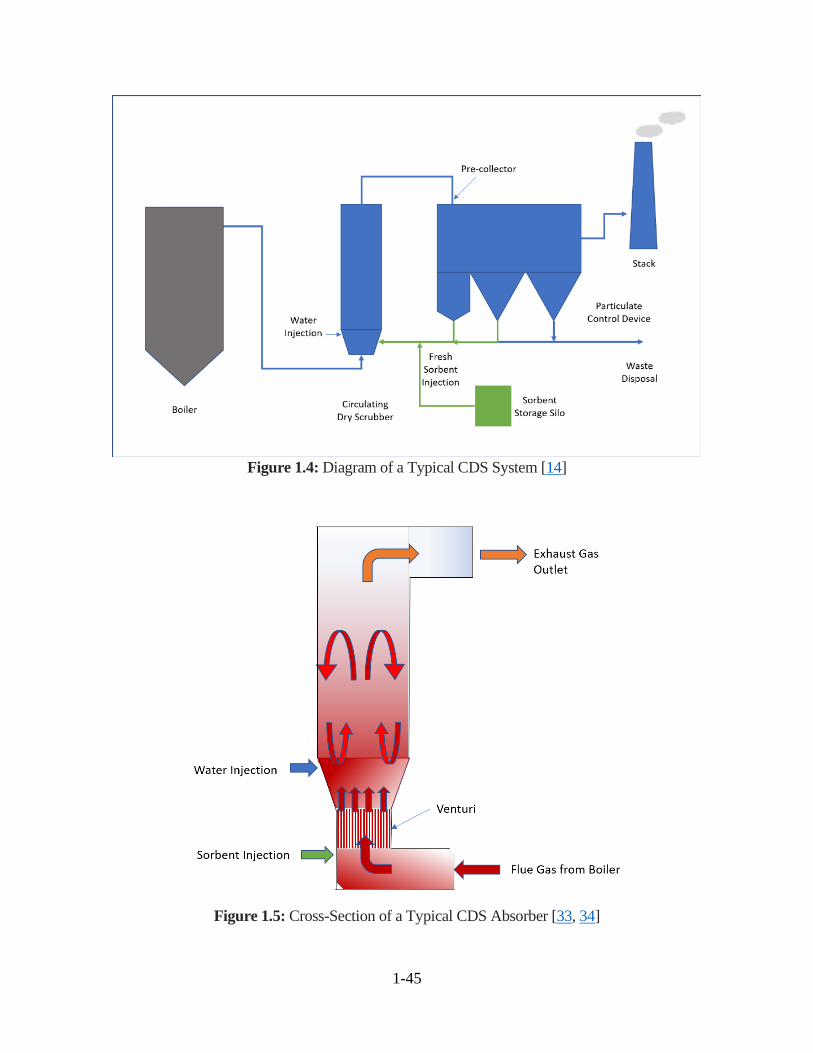
1-45
Figure 1.4: Diagram of a Typical CDS System [14]
Figure 1.5: Cross-Section of a Typical CDS Absorber [33, 34]

1-46
Types of Sorbent
Dry FGD systems may use either calcium or sodium-based carbonates as sorbent
reagents. However, lime is the most commonly used sorbent in SDA and CDS systems. FGD
systems using lime typically add a small amount of water to improve removal efficiency.
Hydrated lime increases the ash resistivity and the injected sorbent adds to the particulate loading
of the precipitator or filter bag system.
System Efficiencies and Performance
The suitability and costs of dry FGD systems as pollution control methods are generally
dependent on the following factors:
1) unit size;
2) required removal efficiency;
3) inlet pollutant (e.g. chlorides, sulfur and mercury) concentrations;
4) anticipated capacity factor; and
5) available space.
1.2.5.2 Design Criteria
The capital and operating cost for a dry FGD system varies depending on the following
factors:
1) Original equipment installation or retrofit of existing boiler/furnace;
2) permitted emission rates for HCl, SO2, SO3, NOX, and Hg;
3) fuel types and future fuel mix;
4) required removal efficiency; and,
5) selected sorbent and waste disposal cost.
These factors require a design concept that determines not just the current fuel and
operational characteristics but how these might change in future operation.
1.2.5.3 Design Parameters for Study-Level Estimates for SDA FGD Control Systems
Methods for estimating the reagent feed rate, make-up water consumption, waste
generation rate and auxiliary power consumption for an SDA system are presented in this
section. These parameters are used in the cost methodology presented in Section 1.2.4.5 for
estimating the annual operating costs for an SDA system. The methods presented in this section
are those developed by the EPA’s CAMD for the cost methodology used with the IPM. [20]

1-47
Reagent Consumption
The reagent usage is a function of the boiler size, SO2 emission rate and the removal
efficiency of the SDA system. The estimated reagent usage was based on a flue gas temperature
into the SDA system of 300°F and an adiabatic approach to saturation of 30°F. The calcium-to-
sulfur stoichiometric ratio varies based on the inlet sulfur content; however, the variation in
stoichiometric ratio was accounted for in the calculation method. The method is valid only up to
3 lb SO2/MMBtu inlet emission rate. The lime is assumed to be 90% pure CaO, with the balance
being inert material. Since the equation for lime consumption is based on data for systems with a
95% SO2 removal efficiency, the IPM equation has been adjusted for the actual SO2 removal
achieved by the SDA system by the factor EF (removal efficiency)/0.95. The reagent usage rate
is calculated as follows:
𝑄𝐿𝑖𝑚𝑒 =[(0.6702×𝑆2)+(13.42×𝑆)]×𝐴×𝐻𝑅𝐹
2,000×
𝐸𝐹
0.95 (1.33)
Where
QLime = lime consumption rate, tons/hour
S = SO2 emission rate, lb/MMBtu
A = Unit size (Gross), MW
HRF = heat rate factor (calculated using Equation 1.6)
EF = removal efficiency, fraction.
Make-up Water
The makeup water rate is a function of gross unit size (actual gas flow rate) and SO2
emission rate. The make-up water consumption rate for a utility boiler is calculated using the
following equation:
𝑞𝑤𝑎𝑡𝑒𝑟 =[(0.04898×𝑆2)+(0.5925×𝑆)+55.11)]×𝐴×𝐶𝑜𝑎𝑙𝐹×𝐻𝑅𝐹
1,000 (1.34)
Where
qwater = make-up water consumption rate, 1,000 gallons/hour
S = SO2 emission rate, lb/MMBtu
A = Unit size (Gross), MW
CoalF = coal factor (CoalF = 1 if bituminous; CoalF = 1.05 if PRB; CoalF = 1.07 if
Lignite)
HRF = heat rate factor (calculated using Equation 1.6).
Waste Generation Rate
The design waste generation rate for SDA systems can be calculated as follows:
𝑞𝑤 = (0.8016×𝑆2+31.1917×𝑆)×𝐴×𝐻𝑅𝐹
2,000×
𝐸𝐹
0.95 (1.35)

1-48
Where:
qw = waste generation rate, tons/hour
S = SO2 emission rate, lb/MMBtu
A = Unit size (Gross), MW
HRF = heat rate factor (calculated using Equation 1.6)
EF = SO2 removal efficiency, fraction
0.95 = SO2 removal efficiency basis for model.
Auxiliary Power Costs
The additional auxiliary power required for the SDA system in kilowatts (kW) is
estimated as a percent of the total unit gross production.
𝑃 = ([(0.000547 × 𝑆2) + (0.00649 × 𝑆) + 1.3] × 𝐶𝑜𝑎𝑙𝐹 × 𝐻𝑅𝐹)/100 × 𝐴 × 1,000 (1.36)
Where:
P = electrical power consumption of the SDA system, kW
S = SO2 emission rate, lb/MMBtu
0.000547 = constant
0.00649 = constant
A = Unit size (Gross), MW
CoalF = coal factor (CoalF = 1 if bituminous; CoalF = 1.05 if PRB; CoalF = 1.07 if
lignite)
HRF = heat rate factor (calculated using Equation 1.6)
100 = conversion factor, percent to decimal fraction
1,000 = conversion factor, kW/MW.
1.2.5.4 Capital Costs for SDA Control Systems
This section presents a methodology for estimating the capital and annual costs for SDA
systems. The cost equations are based on those developed by the EPA’s CAMD as part of the
IPM version 6 (IPM v6). [20] The methodology provides an approach for estimating study-level
capital and annual costs. The capital costs are in 2016 dollars. The IPM algorithms are based on
cost data from S&L’s in-house database of SDA projects and various industry publications. [20] The
capital cost algorithms are valid for units of 50 MW or more. Capital costs for units smaller than 50
MW are approximately $1,000/kW.
The IPM does not provide cost equations for CDS systems; however, the capital costs for
a CDS system are similar to the SDA system for a combustion unit of the same size and sulfur
emission rate.
The IPM is based primarily on data for retrofits, which are typically 30% more than for
new units of the same size and design. To correct for the additional costs associated with
retrofits, we have included a retrofit factor in the TCI equations. A retrofit factor (RF) of 0.77
should be used for new construction and a retrofit factor of 1 should be used for retrofits to
existing units, where the retrofit is of an average level of difficulty. Retrofit costs vary

1-49
significantly from site to site and depend on the amount of space available and whether
modifications to existing equipment (e.g., ductwork, stack) are necessary. A higher retrofit factor
should be used for sites that are congested or where extensive modifications are required for
existing systems.
The capital cost equations are presented in this Section 1.2.4.4 and the methods for
estimating the annual costs are provided in Section 1.2.4.5. The total capital investment (TCI)
includes direct and indirect costs associated with purchasing and installing the control
equipment. TCI includes the equipment cost for the SDA, the cost of auxiliary equipment, the
cost of a fabric filter/baghouse, direct and indirect installation costs, costs for buildings and site
preparation, cost of land and working capital. The capital costs assume the installation is
completed using multiple lump sum contracts. Costs for turnkey (where the project price is fixed
at the time a construction contract is signed) engineering procurement construction contracts may
be 10% to 15% higher than those calculated using the IPM equations. [20]
The TCI does not include the owner’s costs (for owner activities related to engineering,
management, and procurement) and costs such as allowance for funds used during construction
(AFUDC). Although these are capital cost items included in the IPM cost estimates, they are
excluded from the cost methodologies presented in the EPA Control Cost Manual because they
are inconsistent with the overnight cost method9 that is a key basis for the Control Cost Manual
methodology. A more detailed discussion of capital costs can be found in Section 1, Chapter 2 of
this Manual.
Table 1.5 shows the installed costs reported to the U.S. Department of Energy, Energy
Information Administration (EIA). The EIA data includes dry scrubbers with a removal
efficiency of 80% or greater. Table 1.5 also shows the capital costs estimated for an SDA and
CDS system installed on a 500 MW unit calculated using the IPM methodology. For the SDA
and CDS systems, the IPM estimates are higher than the average costs but are well below the
highest costs reported to EIA.
Table 1.5: Comparison of the IPM Capital Cost Methodology Against Installed Costs Reported to the
Energy Information Administration [18]
Fuel Type
Scrubber
Type
EIA Cost Data IPM TCI
Median
$/KWh
Average
$/KWh
Minimum
$/KWh
Maximum
$/KWh
Estimated
$/KWh
Subbituminous CDS 215 281 65 665 499
Bituminous CDS 248 288 182 434 No data
9 The overnight cost estimation method presumes costs are incurred as if the project in question incurred no interest
during construction, or was built “overnight.” Another description of this method is the present value cost that would
have to be paid as a lump sum up front to completely pay for a construction project. For more information, see
“Conducting Technical and Economic Evaluations – As Applied for the Process and Utility Industries,”
Recommended Practice 16R-90, American Association of Cost Engineering International. April 1991, or Section 1,
Chapter 2 of this Control Cost Manual.

1-50
Subbituminous SDA 178 220 19 606 499
Bituminous SDA 188 377 135 923 No data
Total Capital Investment for SDA FGD Control Systems
The equipment required for an SDA system using lime as sorbent varies by the pollutant
and the emission requirements of the source. The algorithms presented in this section are based
on the typical SDA system and are appropriate for facilities that are using coal types with less
than 3 lb SO2/MMBtu achieving a removal efficiency of 95%.
The typical SDA system using pebble lime consists of:
1) Receiving and storage silos;
2) Conveying equipment for lime unloading;
3) Lime feeder;
4) Lime slaker;
5) Lime slurry tank;
6) Slurry pump;
7) Slurry metering pump;
8) Dust control filtering systems;
9) Spray dryer absorber vessel;
10) Atomizers;
11) Waste extraction system;
12) Compressed air;
13) Valves; and
14) Data Control System.
The total capital investment costs for an SDA system include the costs for the absorber
island, reagent preparation equipment, baghouse, waste recycling/handling facilities, and
additional costs associated with installation. These additional costs of installation are called
“balance of plant (BOP) costs” and include the costs for additional duct work, piping, buildings,
foundations, electrical wiring and booster fans. The TCI calculation for the SDA system includes
a factor of 1.3 to estimate (1) engineering and construction management costs, (2) labor

1-51
adjustment for overtime pay, and (3) contractor profit and fees. Each of these 3 items is
estimated to be 10% of the TCI.
The total capital investment cost for an SDA system is given by the Equation 1.37:
𝑇𝐶𝐼 = 1.3 × (𝐴𝐵𝑆𝐶𝑜𝑠𝑡 + 𝐵𝑀𝐹𝐶𝑜𝑠𝑡 + 𝐵𝑂𝑃𝐶𝑜𝑠𝑡) (1.37)
Where:
TCI = total capital investment for an SDA FGD system, $
ABSCost = cost of the SDA FGD system absorber island, $
BMFCost = reagent preparation and waste recycle/handling equipment cost, $
BOPCost = balance of plant costs, $.
The costs for the absorber island and baghouse (ABSCost), reagent preparation and waste
recycle/handling equipment (BMFcost) and balance of plant costs (BOPCost) are discussed below.
The capital cost for an SDA control system varies depending on the size of the unit. The gross
heat rate impacts the amount of flue gas generated and ultimately impacts the size of the
absorber, reagent preparation, waste handling, and the BOP costs. The SO2 emissions rate
primarily impacts the capital costs of the reagent and waste handling facilities, while the type of
fuel burned impacts the quantity of flue gas and thereby impacts the BOPCost.
The ABSCost and BOPCost are also impacted by the unit’s elevation with respect to sea
level. The original cost calculations were developed for SDA FGD systems located within 500
feet of sea level. Therefore, for SDA FGD systems located at higher elevations, the ABSCost and
BOPCost should be increased by multiplying by the elevation factor, ELEVF, which is calculated
using Equations 1.7 and 1.8 in Section 1.2.2.4. [20]
Capital Costs for Coal-fired Combustion Units >600 MW (6,000 MMBtu/hour)
The capital costs for the SDA FGD system absorber island and baghouse are calculated
as follows:
𝐴𝐵𝑆𝐶𝑜𝑠𝑡 = 𝐴 × 98,000 × 𝐸𝐿𝐸𝑉𝐹 (1.38)
Where:
ABSCost = SDA FGD system absorber island and baghouse costs, $
98,000 = constant
A = Unit size (Gross), MW
ELEVF = elevation factor (calculated using Equations 1.7 and 1.8, if plant is located
above 500 feet above sea level; ELEVF = 1 for plants located at 500 ft above
sea level).
The costs for the reagent preparation and waste recycle/handling costs for SDA FGD
systems greater than 600 MW (6,000 MMBtu/hour) are calculated as follows:
𝐵𝑀𝐹𝐶𝑜𝑠𝑡 = 𝐴 × 52,000 (1.39)
1-52
Where:
BMFCost = reagent preparation and waste recycle/handling cost, $
52,000 = constant in the equation
A = Unit size (Gross), MW.
The balance of plant costs (BOPcost) for coal-fired units > 600 MW (6,000 MMBtu/hour)
include costs for piping, water treatment for dilution water, ductwork, auxiliary power
modifications, and other electrical and site upgrades that are typically necessary as part of the
installation of the SDA FGD system. The BOP costs are calculated as follows:
𝐵𝑂𝑃𝐶𝑜𝑠𝑡 = 138,000 × 𝐴 × 𝐸𝐿𝐸𝑉𝐹 (1.40)
Where:
BOPCost = Balance of plant costs, $
138,000 = constant in the equation
A = Unit size (Gross), MW
ELEVF = elevation factor (calculated using Equations 1.7 and 1.8, if plant is located
above 500 feet above sea level; ELEVF = 1 for plants located at 500 ft above
sea level).
Capital Costs for Coal-fired Combustion Units Between 50 and 600 MW (500 and
6,000 MMBtu/hour)
For coal-fired utility units between 50 and 600 MW (500 to 6,000 MMBtu/hour), the
capital costs for the SDA FGD absorber island vary based on the type of coal burned and the
sulfur dioxide emission rate. The capital costs of the absorber island, including the costs for a
baghouse, are calculated as follows:
𝐴𝐵𝑆𝐶𝑜𝑠𝑡 = 637,000 × (𝐴)0.716 × (𝐶𝑜𝑎𝑙𝐹 × 𝐻𝑅𝐹)0.6 × (𝑆/4)0.01 × 𝐸𝐿𝐸𝑉𝐹 × 𝑅𝐹 (1.41)
Where:
ABSCost = SDA FGD absorber island costs (includes cost of an absorber and a baghouse),
$
637,000 = constant in the equation
A = Unit size (Gross), MW
HRF = heat rate factor
CoalF = coal factor (CoalF = 1 if bituminous; CoalF = 1.05 if PRB; CoalF = 1.07 if
Lignite)
ELEVF = elevation factor (calculated using Equations 1.7 and 1.8, if the plant is located
above 500 feet above sea level; ELEVF = 1 for plants located at as below 500
ft above sea level)
S = SO2 emission rate, lb/MMBtu
RF = retrofit factor (RF = 0.77 for new construction; RF = 1 for retrofits with
average level of difficulty).

1-53
The coal factor, CoalF, depends on the type of coal burned. A factor of 1 is used for
bituminous coal, 1.05 for Powder River Basin (PRB) coal, and 1.07 for lignite coal. The heat rate
factor (HRF) is calculated using Equation 1.6.
The reagent preparation and waste recycle/handling costs (BMFCost) are for SDA FGD
systems between 50 and 600 MW (500 and 6,000 MMBtu/hour) are calculated as follows:
𝐵𝑀𝐹𝐶𝑜𝑠𝑡 = 338,000 × (𝐴)0.716 × (𝑆 × 𝐻𝑅𝐹)0.2 × 𝑅𝐹 (1.42)
Where:
BMFCost = reagent preparation and waste recycle/handling cost, $
338,000 = constant in the equation
HRF = heat rate factor (calculated using Equation 1.6)
S = SO2 emission rate, lb/MMBtu
RF = retrofit factor (RF = 0.77 for new construction; RF = 1 for retrofits with average
level of difficulty)
A = Unit size (Gross), MW.
The balance of plant costs (BOPcost) vary based on the size of the unit, type of coal
burned, and the elevation of the unit. The BOPcost are calculated as follows:
𝐵𝑂𝑃𝐶𝑜𝑠𝑡 = 899,000 × (𝐴)0.716 × (𝐶𝑜𝑎𝑙𝐹 × 𝐻𝑅𝐹)0.4 × 𝐸𝐿𝐸𝑉𝐹 × 𝑅𝐹 (1.43)
Where:
BOPCost = Balance of plant costs, $
899,000 = constant in the equation
A = Unit size (Gross), MW
CoalF = coal factor (CoalF = 1 if bituminous; CoalF = 1.05 if PRB; CoalF = 1.07 if
Lignite)
HRF = heat rate factor (calculated using Equation 1.6)
ELEVF = elevation factor (calculated using Equations 1.7 and 1.8 if plant is located above
500 feet above sea level; ELEVF = 1 for plants located at 500 ft above sea level)
RF = retrofit factor (RF = 0.77 for new construction; RF = 1 for retrofits with average
level of difficulty).
1.2.5.5 Total Annual Costs for SDA Systems
The annual costs for controls comprise of the direct and indirect annual costs. The
methods for estimating the direct annual costs of operating the control system, such as the cost of
reagent and operating labor, are presented in this section. The indirect annual costs are the fixed
costs associated with owning and operating the control system and include the annualized capital
recovery cost and the costs for insurance and overhead. Methods for calculating the indirect costs
also are presented in this section. The methods presented in this section are those developed
specifically for SDA control systems by the EPA’s CAMD for the IPM cost methodology. [20]

1-54
Direct Annual Costs
Direct annual costs (DAC) include variable and semi-variable costs. Variable direct
annual costs account for purchase of reagent, utilities (electrical power and water), and any
additional waste disposal costs resulting from the operation of the dry scrubber. Semi-variable
direct annual costs include operating and supervisory labor and maintenance (labor and
materials). For the SDA FGD system, DAC is calculated as follows:
+
+
−+
+
+
=
Cost
Power
Auxiliary
Annual
Cost
Disposal
Waste
Annual
Cost
Water
upMake
Annual
Cost
Reagent
Annual
Cost
Operator
Annual
Cost
eMaintenanc
Annual
DAC
(1.44)
Annual Maintenance Cost. The annual maintenance cost (AMC) includes the costs for
labor and material. For an SDA FGD system, the AMC is estimated to be 1.5%. This is a standard
percentage for maintenance on emissions control devices. The equation for annual maintenance
cost for an SDA FGD system is given by:
𝐴𝑀𝐶 = 0.015 × 𝑇𝐶𝐼 (1.45)
Annual Operator Cost. Therefore, the cost of operator labor is calculated as follows:
Annual Operator Labor Cost = FT × 2,080 × Hourly Labor Rate (1.46)
where FT is the number of additional full-time personnel required to operate the control
system and 2,080 is the annual number of work hours per full time employee. Generally, eight
additional full-time personnel are required to operate an SDA FGD system.
Annual Reagent Cost. The annual cost of reagent (ARcost) is estimated using the reagent
consumption rate, the total effective operating time (top) and the cost of the reagent (CostLime).
The lime consumption rate (QLime) is calculated using Equation 1.31. The total effective
operating time (top) is calculated using Equations 1.3 through 1.5 in Section 1.2.2.2.
𝐴𝑅𝐶𝑜𝑠𝑡 = 𝑄𝐿𝑖𝑚𝑒 × 𝐶𝑜𝑠𝑡𝐿𝑖𝑚𝑒 × 𝑡𝑜𝑝 (1.47)
Where:
ARcost = annual lime cost, $/year
QLime = reagent consumption rate, tons/hour
CostLime = purchase price of reagent, $/ton.
top = effective number of operating hours, hour/year.
Annual Waste Disposal Cost. Using the estimated waste generation rate calculated in
Equation 1.35, the annual cost of wastewater disposal is given by:
Annual waste disposal cost = qwaste × Costdisposal × top (1.48)

1-55
Where:
qwaste = waste generation rate, tons/hour
Costdisposal = unit cost of waste disposal, $/ton
top = effective number of operating hours, hours/year.
Annual Auxiliary Power Cost. Using the estimated power consumption from Equation
1.36, the annual cost of electricity is calculated as follows:
Annual electricity cost =P × Costelec × top (1.49)
Where:
P = electrical power consumption for the dry scrubber, kW
Costelec = unit price of electricity, $/kWh
top = effective number of operating hours, hours/year.
Annual Make-up Water Cost for SDA Systems. Using the estimated make-up water
consumption rate calculated in Equation 1.34, the annual cost of make-up water in $/yr is given
by:
Annual water cost = qwater × Costwater × top (1.50)
Where:
qwater = make-up water consumption rate, kgallons (1,000 gallons)/hour
Costwater = unit cost of water, $/gallon
top = number of operating hours, hours/year.
Indirect Annual Costs for SDA FGD Control Systems
In general, indirect annual costs are fixed costs that include the capital recovery cost,
property taxes, insurance, administrative charges, and overhead. The capital recovery cost is
based on the anticipated equipment lifetime and the annual interest rate employed. As mentioned
earlier in this chapter, acid gas scrubber systems are expected to have an equipment lifetime of
30 years. However, for retrofits on older combustion units, the remaining life of the controlled
combustion unit may be an important factor for determining the expected lifetime for a dry
scrubber.
For this analysis, taxes are assumed to be zero since property taxes generally do not apply
to air pollution control equipment given that purchase of additional land is unusual for
installation of an add-on control device. Insurance for an absorber system is expected to be
minimal. The cost of overhead for an SDA FGD system is also assumed to be zero since control
systems add only minimal overhead costs to those already incurred by the plant. Overhead
includes payroll overhead (i.e., expenses related to labor employed in operation and maintenance
of hardware) and plant overhead (i.e., costs for plant protection, control laboratories, and parking
areas).

1-56
Using these assumptions, indirect annual costs in $/yr, IDAC, consist of both
administrative charges and capital recovery, which can be expressed as:
IDAC = AC + CR (1.51)
where AC represents the administrative charges and CR represents the capital recovery cost.
Administrative charges may be calculated as:
AC = 0.03 × (Annual Operator Cost + 0.4 x Annual maintenance cost) (1.52)
Capital recovery is estimated as:
CR = CRF × TCI (1.53)
where TCI is the total capital investment in dollars and CRF is the capital recovery factor.
Capital recovery factor is a function of the equipment life and the opportunity cost of the capital
(i.e., interest rate). The CRF is defined as:
𝐶𝑅𝐹 =𝑖(1+𝑖)𝑛
(1+𝑖)𝑛−1 (1.54)
where i is the assumed interest rate and n is the equipment life of the dry scrubber system.
Total Annual Cost
The total annual cost, TAC, for owning and operating a dry scrubber is the sum of direct
and indirect annual costs as given in the following equation:
TAC = DAC + IDAC (1.55)
1.2.5.6 Cost Effectiveness
The cost in dollars per ton of SO2 removed per year, is calculated as follows:
𝐶𝑜𝑠𝑡 𝐸𝑓𝑓𝑒𝑐𝑡𝑖𝑣𝑒𝑛𝑒𝑠𝑠 =𝑇𝐴𝐶
𝑆𝑂2 𝑅𝑒𝑚𝑜𝑣𝑒𝑑/𝑦𝑒𝑎𝑟 (1.56)
Where:
Cost Effectiveness = the cost effectiveness, $/ton
SO2 Removed/year = annual mass of SO2 removed by the absorber, tons/yr
TAC = total annual cost, $/year.
1.2.5.7 Example Problem
This section illustrates how to calculate the design parameters and capital and annual
costs for the retrofit of an existing 500 MW utility boiler burning bituminous coal with an SDA
FGD system. This example is purely illustrative, and is not meant to serve in place of the actual
data on a SDA FGD system that is included in an actual cost analysis.
1-57
Design Basis for Example Project
For the purposes of this example, the 500 MW boiler is located at approximately 500 feet
above sea level and the retrofit is assumed to be of typical complexity with the site having
sufficient space available to install the absorber, reagent preparation and storage, and wastewater
handling facilities. The following assumptions are made to perform the calculations:
Boiler MW rating full load capac 500 MW
Coal consumption rate, qfuel 326,600 lb/hour
High heating value of bituminous coal, HHV 15,000 Btu/lb
Gross heat input rate, GHR 9.8 MMBtu/MWh
Uncontrolled SO2 emission rate, Sin 2.0 lb/MMBtu
Required controlled SO2 emission rate, Sout 0.1 lb/MMBtu
Annual effective operating hours, top 8,000 hours/year
Retrofit factor, RF 1
Elevation factor, ELEVF 1
In addition to these assumptions regarding the physical parameters of the boiler, the
economic factors for the example cost calculations are as follows:
Cost Year 2016
Equipment Life 30 years
Annual Interest Rate10 3.25%
Lime cost11 125 $/ton
Water Consumption Cost12 0.0042 $/gal
Electricity Cost13 0.0361 $/kWh
Waste Disposal Cost15 30 $/ton
Labor rate15 60 $/hour
10 As stated in Section 1, Chapter 2 of the Cost Manual, the interest rate that is appropriate for annualizing capital
cost is either the bank prime rate (currently 3.25%), which is an interest rate set by the Federal Reserve Board that
fluctuates with the market for financial credit, or a firm-specific rate that reflects the rates of debt and equity for the
firm owning the unit at issue if that firm can justify this alternative rate. The bank prime rate serves as a default if
the firm can, or decides not to, provide an interest rate reflecting its rates for debt borrowing and/or equity. 11 U.S. Environmental Protection Agency (EPA). Documentation for EPA’s Power Sector Modeling Platform v6
Using the Integrated Planning Model. Office of Air and Radiation. January 2017. Available at:
https://www.epa.gov/airmarkets/documentation-epas-power-sector-modeling-platform-v6. 12 Average water rates for industrial facilities in 2016 compiled by Black & Veatch. See “50 Largest Cities
Water/Wastewater Rate Survey – 2018-2019.” Available at https://www.bv.com/sites/default/files/2019-
10/50_Largest_Cities_Rate_Survey_2018_2019_Report.pdf. 13 U.S. Energy Information Administration. Electric Power Annual 2016. Table 8.4. Published December 2017.
Available at: https://www.eia.gov/electricity/annual/pdf/epa.pdf.

1-58
Design Parameters for Example Retrofit Project
Boiler Heat Rate. The boiler annual heat input rate, QB, is calculated from the HHV for
bituminous coal given in Table 1.4 and the maximum fuel consumption rate, qfuel, using
Equation 1.1:
𝑄𝐵 =15,000
𝐵𝑡𝑢𝑙𝑏
× 326,600𝑙𝑏ℎ𝑟
106 𝐵𝑡𝑢𝑀𝑀𝐵𝑡𝑢
= 4,899𝑀𝑀𝐵𝑡𝑢
ℎ𝑟
SO2 Removal Efficiency. The SO2 removal efficiency, EF, is calculated from the inlet
SO2 emission level and the required stack SO2 emission level:
𝐸𝐹 = [𝑆𝑂2𝐼𝑛 − 𝑆𝑂2𝑂𝑢𝑡
𝑆𝑂2𝐼𝑛] × 100
𝐸𝐹 = [2.0
𝑙𝑏𝑀𝑀𝐵𝑡𝑢 − 0.10
𝑙𝑏𝑀𝑀𝐵𝑡𝑢
2.0𝑙𝑏
𝑀𝑀𝐵𝑡𝑢
] × 100 = 95%
−
The SO2 removed per hour (lb/hr) is calculated from the inlet SO2 emission level, the SO2
removal efficiency, and the maximum heat rate to the boiler:
SO2 Removed/hr = SO2in x EF x QB
𝑆𝑂𝑥 𝑅𝑒 𝑚 𝑜𝑣𝑒𝑑/ℎ𝑟 = 2.0𝑙𝑏
𝑀𝑀𝐵𝑡𝑢× 0.95 ×
4,899𝑀𝑀𝐵𝑡𝑢
ℎ𝑜𝑢𝑟= 9,308
𝑙𝑏
ℎ𝑟
Reagent Consumption Rate. The lime consumption rate is calculated using Equation
1.33:
𝑄𝐿𝑖𝑚𝑒 =[(0.6702 × 𝑆2) + (13.42 × 𝑆)] × 𝐴 × 𝐻𝑅𝐹
2,000×
𝐸𝐹
0.95
𝑄𝐿𝑖𝑚𝑒 =[(0.6702 × (2.0)2) + (13.42 × 2.0)] × 500 × 0.98
2,000×
0.95
0.95= 7.23 𝑡𝑜𝑛𝑠/ℎ𝑜𝑢𝑟
Make-up Water Consumption. The make-up water consumption rate is calculated using
Equation 1.34:
𝑞𝑤𝑎𝑡𝑒𝑟 =[(0.04898 × 𝑆2) + (0.5925 × 𝑆) + 55.11)] × 𝐴 × 𝐶𝑜𝑎𝑙𝐹 × 𝐻𝑅𝐹
1,000

1-59
𝑞𝑤𝑎𝑡𝑒𝑟 =[(0.04898 × (2.0)2) + (0.5925 × 2.0) + 55.11)] × 500 × 1 × 0.98
1,000= 27.7 𝑘𝑔𝑎𝑙𝑙𝑜𝑛𝑠/ℎ𝑜𝑢𝑟
Waste Generation. Using Equation 1.35, design waste generation rate for SDA systems
can be calculated as follows:
qwaste = (0.8016 × S2 + 31.1917 × S) × A × HRF
2,000×
EF
0.95
𝑞𝑤𝑎𝑠𝑡𝑒 = [0.8016×(2.0)2+(31.1917×2.0)]×500×0.98
2,000×
0.95
0.95= 16.1 𝑡𝑜𝑛𝑠/ℎ𝑜𝑢𝑟
Electricity Consumption. The auxiliary power required for the SDA FGD is estimated
using Equation 1.36:
P = ([(0.000547 × S2) + (0.00649 × S) + 1.3] × CoalF × HRF)/100 × A × 1,000
𝑃 = ([(0.000547 × (2.0)2) + (0.00649 × 2.0) + 1.3] × 1 × 0.98)/100 × 500 × 1,000
𝑃 = 6,444 𝑘𝑊
Cost Estimation for Example Retrofit Project
Once the SDA FGD system is sized, the capital and annual costs can be estimated. The
total capital investment costs (TCI) are estimated using Equation 1.37:
𝑇𝐶𝐼 = 1.3 × (𝐴𝐵𝑆𝐶𝑜𝑠𝑡 + 𝐵𝑀𝐹𝐶𝑜𝑠𝑡 + 𝐵𝑂𝑃𝐶𝑜𝑠𝑡)
Where:
TCI = total capital investment for an SDA FGD system, $
ABSCost = cost of the SDA FGD system absorber island and baghouse, $
BMFCost = reagent preparation and waste recycle/handling equipment cost, $
BOPCost = balance of plant costs, $.
The capital costs for the absorber island and baghouse are estimated using Equation 1.38:
𝐴𝐵𝑆𝐶𝑜𝑠𝑡 = 637,000 × (𝐴)0.716 × (𝐶𝑜𝑎𝑙𝐹 × 𝐻𝑅𝐹)0.6 × (𝑆/4)0.01 × 𝐸𝐿𝐸𝑉𝐹 × 𝑅𝐹
𝐴𝐵𝑆𝐶𝑜𝑠𝑡 = 637,000 × (500)0.716 × (1.0 × 0.98)0.6 × (2/4)0.01 × 1 × 1 = $53,496,738
The costs for the reagent preparation and waste recycle/handling costs can be calculated
using Equation 1.39:
𝐵𝑀𝐹𝐶𝑜𝑠𝑡 = 338,000 × (𝐴)0.716 × (𝑆 × 𝐻𝑅𝐹)0.2 × 𝑅𝐹
𝐵𝑀𝐹𝐶𝑜𝑠𝑡 = 338,000 × (500)0.716 × (2.0 × 0.98)0.2 × 1 = $33,100,186

1-60
The BOPCost can be calculated using Equation 1.40:
𝐵𝑂𝑃𝐶𝑜𝑠𝑡 = 899,000 × (𝐴)0.716 × (𝐶𝑜𝑎𝑙𝐹 × 𝐻𝑅𝐹)0.4 × 𝐸𝐿𝐸𝑉𝐹 × 𝑅𝐹
𝐵𝑂𝑃𝐶𝑜𝑠𝑡 = 899,000 × (500)0.716 × (1 × 0.98)0.4 × 1 × 1 = $76,333,055
The total capital investment can be calculated using the values above:
𝑇𝐶𝐼 = 1.3 × ($53,496,738 + $33,100,186 + $76,333,055) = $211,808,973
Assuming the effective operating hours for the SDA FGD system are 8,000 hours per
year, then the annual variable costs for maintenance, operator labor, reagent, waste, auxiliary
power, and make-up water can be calculated using Equations 1.45, 1.46, 1.47, 1.48, 1.49 and
1.50, respectively.
𝐴𝑛𝑛𝑢𝑎𝑙𝑀𝑎𝑖𝑛𝑡𝑒𝑛𝑎𝑛𝑐𝑒𝐶𝑜𝑠𝑡(𝐴𝑀𝐶) = 0.015 × $211,808,973 = $3,177,135
Annual Operator Labor Cost = 8 × 2080 hours/year× $60/hour = $998,400
𝐴𝑛𝑛𝑢𝑎𝑙 𝑟𝑒𝑎𝑔𝑒𝑛𝑡 𝑐𝑜𝑠𝑡 = 7.23𝑡𝑜𝑛𝑠
ℎ𝑜𝑢𝑟× 125
$
𝑡𝑜𝑛× [8,000
ℎ𝑟𝑠
𝑦𝑟] = $7,232,596
𝐴𝑛𝑛𝑢𝑎𝑙 𝑤𝑎𝑠𝑡𝑒 𝑑𝑖𝑠𝑝𝑜𝑠𝑎𝑙 𝑐𝑜𝑠𝑡 = 16.1𝑡𝑜𝑛𝑠
ℎ𝑜𝑢𝑟× 30
$
𝑡𝑜𝑛× [8,000
ℎ𝑟𝑠
𝑦𝑟] = $3,856,680
𝐴𝑛𝑛𝑢𝑎𝑙 𝑒𝑙𝑒𝑐𝑡𝑟𝑖𝑐𝑖𝑡𝑦 𝑐𝑜𝑠𝑡 = 6,444𝑘𝑊 × 0.0361$
𝑘𝑊ℎ[8,000
ℎ𝑟𝑠
𝑦𝑟] = $1,861,121
𝐴𝑛𝑛𝑢𝑎𝑙 𝑤𝑎𝑡𝑒𝑟 𝑐𝑜𝑠𝑡 = 27.7𝑘𝑔𝑝ℎ ×1,000𝑔𝑎𝑙
𝑘𝑔𝑎𝑙× 0.0042
$
𝑔𝑎𝑙× [8,000
ℎ𝑟𝑠
𝑦𝑟] = $930,067
The total direct annual cost (DAC), the sum of the cost of the maintenance, labor,
reagent, waste disposal, auxiliary power, and make-up water is given by the sum of the annual
costs:
𝐷𝐴𝐶 = $3,177,135 + $998,400 + $7,232,596 + $3,856,680 + $1,861,121 + $930,067= $18,055,998
Property taxes and overhead are both assumed to be zero, and insurance costs are
assumed to be negligible. Thus, administrative charges and capital recovery are the only
components of indirect annual costs estimated in this analysis. Administrative charges are
calculated using Equation 1.52 as:
Annual Administrative Cost = 0.03 × ($998,400 + 0.4 × $3,177,135) = $68,078
The capital recovery factor, CRF, is a function of the equipment life (30 years) and the
opportunity cost of the capital (i.e., interest rate), defined in Equation 1.54:

1-61
𝐶𝑅𝐹 =0.0325 (1 + 0.0325)30
(1 + 0.0325)30 − 1= 0.0527
The capital recovery is calculated using Equation 1.53 as follows:
CR = 0.0527 × $211,808,973 = $11,162,333/year
The total indirect annual costs (IDAC) are calculated in Equation 1.51:
𝐼𝐷𝐴𝐶 = 𝐴𝐶 + 𝐶𝑅 = $68,078 + $11,162,333 = $11,230,411
The total annual cost is the sum of the direct and indirect annual costs:
𝑇𝐴𝐶 = 𝐷𝐴𝐶 + 𝐼𝐷𝐴𝐶 = $18,055,998 + $11,230,333 = $29,286,408
The total amount of SO2 removed is calculated as follows:
𝐴𝑛𝑛𝑢𝑎𝑙 𝑆𝑂2 𝑅𝑒𝑚𝑜𝑣𝑒𝑑 =2.0
𝑙𝑏
𝑀𝑀𝐵𝑡𝑢×0.95×4,900
𝑀𝑀𝐵𝑡𝑢
ℎ𝑟× 8,000
ℎ𝑟𝑠
𝑦𝑟
2,000𝑙𝑏
𝑡𝑜𝑛
= 37,232 𝑡𝑜𝑛𝑠/𝑦𝑒𝑎𝑟
The annual cost in terms of SO2 removed, or cost effectiveness, for the SDA retrofit is
calculated using Equation 1.56:
𝐴𝑛𝑛𝑢𝑎𝑙 𝐶𝑜𝑠𝑡 𝐸𝑓𝑓𝑒𝑐𝑡𝑖𝑣𝑒𝑛𝑒𝑠𝑠 =$29,286,408
37,232 𝑡𝑜𝑛𝑠= $787/𝑡𝑜𝑛
1.3 Wet Packed Tower Gas Absorbers
Packed tower absorbers are the most common approach to removing acidic gases from
flue gas. The large wetted area provided by the packing makes it possible to achieve very high
removal efficiencies at a relatively low capital and operating costs. In this section, we describe
the process, outline how to determine the critical design characteristics, and provide a method for
estimating the capital and operating costs. The methods outlined in this section can be used for
estimating costs for packed tower absorbers used to control flue gas containing any acidic
pollutants, such as HCl and HF. The method can be used as an alternative approach to the
method provided in Section 1.2.3 for estimating capital and operating costs for packed tower
FGD systems.
1.3.1 Process Description
1.3.1.1 Packed Tower Designs
A basic packed tower absorber is comprised of a column shell, mist eliminator, liquid
distributors, packing materials, packing support, and may include a packing restrainer. Corrosion
resistant alloys or plastic materials such as polypropylene are required for column internals when
highly corrosive solvents or gases are used. A schematic drawing of a countercurrent packed

1-62
tower is shown in Figure 1.6. In this figure, the packing is separated into two sections. This
configuration is more expensive than designs where the packing is not so divided.[6]
Figure 1.6: Packed Tower for Gas Absorption
The tower shell may be made of steel or plastic, or a combination of these materials
depending on the corrosiveness of the gas and liquid streams, and the process operating
conditions. One alloy that is chemical and temperature resistant or multiple layers of different,
less expensive materials may be used. The shell is sometimes lined with a protective membrane,
often made from a corrosion resistant polymer. For absorption involving acid gases, an interior
layer of acid resistant brick provides additional chemical and temperature resistance.[36]
At high gas velocities, the gas exiting the top of the column may carry droplets of liquid
as a mist. To prevent this, a mist eliminator in the form of corrugated sheets or a layer of mesh
can be installed at the top of the column to collect the liquid droplets, which coalesce and fall
back into the column.
A liquid distributor is designed to wet the packing bed evenly and initiate uniform contact
between the liquid and vapor. The liquid distributor must spread the liquid uniformly, resist
plugging and fouling, provide free space for gas flow, and allow operating flexibility.[37] Large
towers frequently have a liquid redistributor to collect liquid off the column wall and direct it
toward the center of the column for redistribution and enhanced contact in the lower section of
packing.[7] Liquid redistributors are generally required for every 8 to 20 feet of random packing
depth.[6, 38]
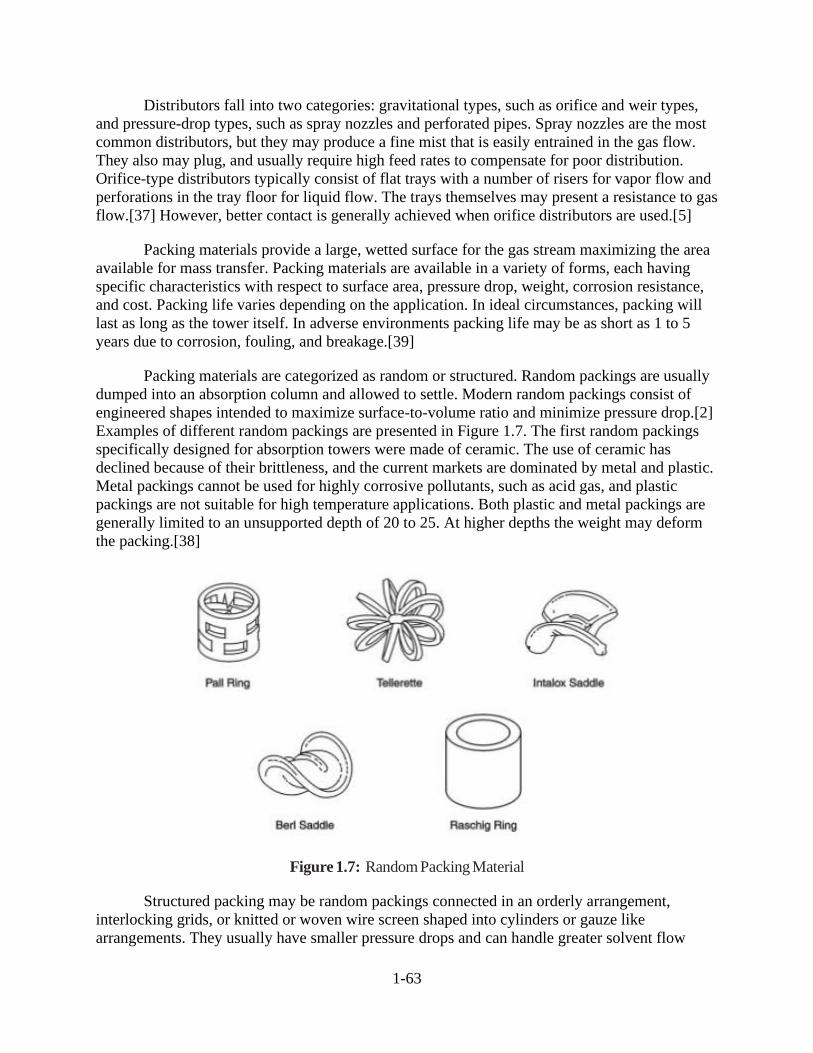
1-63
Distributors fall into two categories: gravitational types, such as orifice and weir types,
and pressure-drop types, such as spray nozzles and perforated pipes. Spray nozzles are the most
common distributors, but they may produce a fine mist that is easily entrained in the gas flow.
They also may plug, and usually require high feed rates to compensate for poor distribution.
Orifice-type distributors typically consist of flat trays with a number of risers for vapor flow and
perforations in the tray floor for liquid flow. The trays themselves may present a resistance to gas
flow.[37] However, better contact is generally achieved when orifice distributors are used.[5]
Packing materials provide a large, wetted surface for the gas stream maximizing the area
available for mass transfer. Packing materials are available in a variety of forms, each having
specific characteristics with respect to surface area, pressure drop, weight, corrosion resistance,
and cost. Packing life varies depending on the application. In ideal circumstances, packing will
last as long as the tower itself. In adverse environments packing life may be as short as 1 to 5
years due to corrosion, fouling, and breakage.[39]
Packing materials are categorized as random or structured. Random packings are usually
dumped into an absorption column and allowed to settle. Modern random packings consist of
engineered shapes intended to maximize surface-to-volume ratio and minimize pressure drop.[2]
Examples of different random packings are presented in Figure 1.7. The first random packings
specifically designed for absorption towers were made of ceramic. The use of ceramic has
declined because of their brittleness, and the current markets are dominated by metal and plastic.
Metal packings cannot be used for highly corrosive pollutants, such as acid gas, and plastic
packings are not suitable for high temperature applications. Both plastic and metal packings are
generally limited to an unsupported depth of 20 to 25. At higher depths the weight may deform
the packing.[38]
Figure 1.7: Random Packing Material
Structured packing may be random packings connected in an orderly arrangement,
interlocking grids, or knitted or woven wire screen shaped into cylinders or gauze like
arrangements. They usually have smaller pressure drops and can handle greater solvent flow

1-64
rates than random packings.[7] However, structured packings are more costly to install and may
not be practical for smaller columns. Most structured packings are made from metal or plastic.
To ensure the waste gas is well distributed, an open space between the bottom of the
tower and the packing is necessary. Support plates hold the packing above the open space. The
support plates must have enough strength to carry the weight of the packing, and enough free
area to allow solvent and gas to flow with minimum restrictions.[7]
High gas velocities can fluidize packing on top of a bed. The packing could then be
carried into the distributor, become unleveled, or be damaged.[37] A packing restrainer may be
installed at the top of the packed bed to contain the packing. The packing restrainer may be
secured to the wall so that column upsets will not dislocate it, or a “floating” unattached
weighted plate may be placed on top of the packing so that it can settle with the bed. The latter is
often used for fragile ceramic packing.
1.3.1.2 Packed Tower Operation
As discussed in Section 1.3.1.1, the most common packed tower designs are
countercurrent. As the waste gas flows up the packed column it will experience a drop in its
pressure as it meets resistance from the packing materials and the solvent flowing down.
Pressure drop in a column is a function of the gas and liquid flow rates and properties of the
packing elements, such as surface area and free volume in the tower. A high pressure drop results
in high fan power to drive the gas through the packed tower and consequently higher costs. The
pressure drop in a packed tower generally ranges from 0.5 to 1.0 in. H2O/ft of packing.[8]
For each column, there are upper and lower limits to solvent and vapor flow rates that
ensure satisfactory performance. The gas flow rate may become so high that the drag on the
solvent is sufficient to keep the solvent from flowing freely down the column. Solvent begins to
accumulate and blocks gas flow in the entire cross-section, which increases the pressure drop and
prevents the packing from mixing the gas and solvent effectively.
When all the free volume in the packing is filled with liquid and the liquid is carried back
up the column, the absorber is considered to be flooded.[7] Most packed towers operate at 60 to
70% of the gas flooding velocity, as it is not practical to operate a tower in a flooded
condition.[8] A minimum liquid flow rate is also required to wet the packing material
sufficiently for effective mass transfer to occur between the gas and liquid.[8]
The waste gas inlet temperature is another important parameter. In general, the higher the
gas temperature, the lower the absorption rate, and vice-versa. Excessively high gas temperatures
also can lead to significant solvent loss through evaporation. Consequently, precoolers (e.g.,
spray chambers) may be needed to reduce the air temperature to acceptable levels.[4]
For operations that are based on chemical reaction with absorption, an additional concern
is the rate of reaction between the solvent and pollutant(s). Most gas absorption chemical
reactions are relatively fast and the rate limiting step is the physical absorption of the pollutants
into the solvent. However, for solvent-pollutant systems where the chemical reaction is the
limiting step, the rates of reaction would need to be analyzed kinetically.

1-65
Heat may be generated as a result of exothermal chemical reactions. Heat may also be
generated when large amounts of solute are absorbed into the liquid phase, due to the heat of
solution. The resulting change in temperature along the height of the absorber column may
damage equipment and reduce absorption efficiency. This problem can be avoided by adding
cooling coils to the column.[8] However, in those systems where water is the solvent, adiabatic
saturation of the gas occurs during absorption due to solvent evaporation. This causes a
substantial cooling of the absorber that offsets the heat generated by chemical reactions. Thus,
cooling coils are rarely required with those systems.[6] In any event, packed towers may be
designed assuming that isothermal conditions exist throughout the column.[8]
The effluent from the column may be recycled into the system and used again. This is
usually the case if the solvent is costly, e.g., hydrocarbon oils or caustic solution. Initially, the
recycle stream may go to a waste treatment system to remove the pollutants or the reaction
product. Make-up solvent may then be added before the liquid stream re-enters the column.
Recirculation of the solvent requires a pump, solvent recovery system, solvent holding and
mixing tanks, and any associated piping and instrumentation.
1.3.2 Design Procedures for Packed Tower Absorbers
The design of packed tower absorbers for controlling gas streams containing a mixture of
pollutants and air depends on knowledge of the following parameters:
• Waste gas flow rate
• Waste gas composition and concentration of the pollutants in the gas stream
• Required removal efficiency
• Equilibrium relationship between the pollutants and solvent
• Properties of the pollutant(s), waste gas, and solvent: diffusivity, viscosity, density, and
molecular weight.
The primary objectives of the design procedures are to determine column surface area
and pressure drop through the column. The following steps are used to determine the surface area
and pressure drop:
• Determine the gas and liquid stream conditions entering and exiting the column.
• Determine the absorption factor (AF).
• Determine the diameter of the column (D).
• Determine the tower height (Htower) and surface area (S).
• Determine the packed column pressure drop (P).
To simplify the sizing procedures, a number of assumptions have been made. For
example, the waste gas is assumed to comprise a two-component waste gas mixture
(pollutant/air), where the pollutant consists of a single compound present in dilute quantities. The
waste gas is assumed to behave as an ideal gas and the solvent is assumed to behave as an ideal
solution. Heat effects associated with absorption are considered to be minimal for the pollutant
concentrations encountered. The procedures also assume that, in chemical absorption, the
process is not reaction rate limited, i.e., the reaction of the pollutant with the solvent is
considered fast compared to the rate of absorption of the pollutant into the solvent.

1-66
The design procedures presented here are complicated, and careful attention to units is
required. A list of all design variables referred to in in the following sections and their
appropriate measurement units is provided in Appendix A, Table A-3.
1.3.2.1 Determining Gas and Liquid Stream Conditions
Gas absorbers are designed based on the ratio of liquid to gas entering the column (Li/Gi),
slope of the equilibrium curve (m), and the desired removal efficiency (η). These factors are
calculated from the inlet and outlet gas and liquid stream variables:
• Waste gas flow rate, in actual cubic feet per minute (acfm), entering and exiting column
(Gi and Go, respectively)
• Pollutant concentration (lb-moles pollutant per lb-mole of pollutant free gas) entering and
exiting the column in the waste gas (Yi and Yo, respectively)
• Solvent flow rate, in gallons per minute (gpm), entering and exiting the column (Li and
Lo, respectively)
• Pollutant concentration (lb-moles pollutant per lb-mole of pollutant free solvent) entering
and exiting the column in the solvent (Xi and Xo, respectively)
For this design approach, we assume the inlet gas stream variables are known, and that a
specific pollutant removal efficiency has been chosen as the design basis (i.e., the variables Gi,
Yi, and η are known). For the dilute concentrations typically encountered in pollution control
applications and negligible changes in moisture content, Gi is assumed equal to Go. If a once-
through process is used, or if the spent solvent is regenerated by an air stripping process before it
is recycled, the value of Xi will approach zero. The remaining stream variables (Yo, Li Lo, and
Xo), the following procedures must be followed. A schematic diagram of a packed tower with
inlet and outlet flow and concentration variables labeled is presented in Figure 1.7.

1-67
Figure 1.8: Schematic Diagram of Countercurrent Packed Bed Operation
The exit pollutant concentration may be calculated using the following equation:
𝑌𝑜 = 𝑌𝑖 (1 −𝜂
100) (1.57)
The liquid flow rate entering the absorber, Li (gpm), is then calculated using a graphical
method. Figure 1.8 presents an example of an equilibrium curve and operating line. The
equilibrium curve indicates the relationship between the concentration of pollutant in the waste
gas and the concentration of pollutant in the solvent at a specified temperature. The operating
line indicates the relationship between the concentration of the pollutant in the gas and solvent at
any location in the gas absorber column. The vertical distance between the operating line and
equilibrium curve indicates the driving force for diffusion of the pollutant between the gas and
liquid phases. The minimum amount of liquid which can be used to absorb the pollutant in the
gas stream corresponds to an operating line drawn from the outlet concentration in the gas stream
(Yo) and the inlet concentration in the solvent stream (Xi) to the point on the equilibrium curve
corresponding to the entering pollutant concentration in the gas stream (Yi). At the intersection
point on the equilibrium curve, the diffusional driving forces are zero, the required time of
contact for the concentration change is infinite, and an infinitely tall tower results.

1-68
Figure 1.9: Minimum and Actual Liquid-to-Gas Ratio.
The slope of the operating line intersecting the equilibrium curve is equal to the minimum
L/G ratio on a moles of pollutant-free solvent (Ls) per moles of pollutant-free gas basis Gs. In
other words, the values Ls and Gs do not include the moles of pollutant in the liquid and gas
streams. The values of Ls and Gs are constant through the column if a negligible amount of
moisture is transferred from the liquid to the gas phase. The slope may be calculated from the
following equation:
(𝐿𝑠
𝐺𝑠)
𝑚𝑖𝑛=
𝑌𝑖−𝑌𝑜
𝑋𝑜∗ − 𝑋𝑖
(1.58)
where X*o would be the maximum concentration of the pollutant in the liquid phase if it were
allowed to come to equilibrium with the pollutant entering the column in the gas phase, Yi. The
value of X*o is taken from the equilibrium curve. Because the minimum Ls/Gs, ratio is an
unrealistic value, it must be multiplied by an adjustment factor, commonly between 1.2 and 1.5,
to calculate the actual L/G ratio:[8]
(𝐿𝑠
𝐺𝑠)
𝑎𝑐𝑡= (
𝐿𝑠
𝐺𝑠)
𝑚𝑖𝑛× (𝑎𝑑𝑗𝑢𝑠𝑡𝑚𝑒𝑛𝑡 𝑓𝑎𝑐𝑡𝑜𝑟) (1.59)
The variable Gs may be calculated using the equation:
𝐺𝑠 =60𝜌𝐺𝐺𝑖
𝑀𝑊𝐺(1+𝑌𝑖) (1.60)

1-69
where 60 is the conversion factor from minutes to hours, MWG, is the molecular weight of the
gas stream (lb/lb-mole), and ρG is the density of the gas stream (lb/ft3). For pollutant
concentrations typically encountered, the molecular weight and density of the waste gas stream
are assumed to be equal to that of ambient air.
The variable Ls may then be calculated by:
𝐿𝑠 = (𝐿𝑠
𝐺𝑠)
𝑎𝑐𝑡× 𝐺𝑠 (1.61)
The total molar flow rates of the gas and liquid entering the absorber (Gmol,i and Lmol,i) are
calculated using the following equations:
𝐺𝑚𝑜𝑙,𝑖 = 𝐺𝑠(1 + 𝑌𝑖) (1.62)
𝐿𝑚𝑜𝑙,𝑖 = 𝐿𝑠(1 + 𝑋𝑖) (1.63)
The volume flow rate of the solvent, Li, may then be calculated by using the following
relationship:
𝐿𝑖 =7.48𝐿𝑚𝑜𝑙,𝑖𝑀𝑊𝐿
60𝑟𝐿 (1.63)
where 60 is the conversion factor from minutes to hours, MWL, is the molecular weight of the
liquid stream (lb/lb-mole), ρL is the density of the liquid stream (lb/ft3), and 7.48 is the factor
used to convert cubic feet to gallons. If the volume change in the liquid stream entering and
exiting the absorber is assumed to be negligible, then Li = Lo.
Gas absorber vendors have provided a range for the Li/Gi ratio for acid gas control from 2
to 20 gpm of solvent per 1000 cfm of waste gas.[40] Even for pollutants that are highly soluble
in a solvent (e.g., HCl in water), the adjusted Li/Gi ratio calculated using Equations 1.59 to 1.64
would be much lower than this range, because these equations do not consider the flow rate of
the solvent required to wet the packing.
Finally, the actual operating line may be represented by a material balance equation over
the gas absorber:[7]
𝑋𝑖𝐿𝑠 + 𝑌𝑖𝐺𝑠 = 𝑋𝑜𝐿𝑠 + 𝑌𝑜𝐺𝑠 (1.65)
Equation 1.65 may then be solved for Xo:
𝑋𝑜 =𝑌𝑖−𝑌𝑜
(𝐿𝑠𝐺𝑠
)+ 𝑋𝑖 (1.66)
1.3.2.2 Determining Absorption Factor
The absorption factor (AF) value is frequently used to describe the relationship between
the equilibrium line and the liquid-to-gas ratio. For many pollutant-solvent systems, the most

1-70
economical value for AF ranges around 1.5 to 2.0.[25] The following equation may be used to
calculate AF: [7, 8]
𝐴𝐹 =𝐿𝑚𝑜𝑙,𝑖
𝑚𝐺𝑚𝑜𝑙,𝑖 (1.67)
where m is the slope of the equilibrium line on a mole fraction basis. The value of m may be
obtained from available literature on vapor/liquid equilibrium data for specific systems. Since the
equilibrium curve is typically linear in the concentration ranges usually encountered in air
pollution control, the slope, m would be constant (or nearly so) for all applicable inlet and outlet
liquid and gas streams. The slope may be calculated from mole fraction values using the
following equation:[7]
𝑚 =𝑦𝑜
∗−𝑦𝑖∗
𝑥𝑜−𝑥𝑖 (1.68)
where y*i and y*
o are the mole fractions of the pollutant in the vapor phase in equilibrium with
the mole fractions of the pollutant entering and exiting the absorber in the liquid, xi and xo,
respectively. The slope of the equilibrium line in Figure 1.8 is expressed in terms of
concentration values Xi, Xo, Y*i, and Y*o. These values may be converted to xi, xo, y*i, and y*o
using the equations:
𝑥𝑖 =𝑋𝑖
1+𝑋𝑖 (1.69)
𝑥𝑜 =𝑋𝑜
1+𝑋𝑜 (1.70)
𝑦𝑖∗ =
𝑌𝑖∗
1+𝑌𝑖∗ (1.71)
𝑦𝑜∗ =
𝑌𝑜∗
1+𝑌𝑜∗ (1.72)
where the units for each of these variables are listed in Appendix A, Table A-3.
The absorption factor (AF) is used to calculate the theoretical number of transfer units
and the theoretical height of a transfer unit. First, however, the column diameter must be
determined.
1.3.2.3 Determining Column Diameter
Once stream conditions have been determined, the diameter of the column may be
estimated. The design presented in this section is based on selecting a fraction of the gas flow
rate at flooding conditions. Alternatively, the column may be designed for a specific pressure
drop (see Section 1.3.2.6). Eckert’s modification to the generalized correlation for randomly
packed towers based on flooding considerations is used to obtain the superficial gas flow rate
entering the absorber, Gsfr,i (lb/sec-ft2), or the gas flow rate per cross-sectional area based on the
Lmol,i/Gmol,i ratio calculated in Section 1.3.2.2.[38] The cross-sectional area (A) of the column
and the column diameter (D) can then be determined from Gsfr,i. Figure 1.9 presents the

1-71
relationship between Gsfr,i and the Lmol,i/Gmol,i ratio at the tower flood point. The Abscissa value
(X axis) in the graph is expressed as:[38]
𝐴𝑏𝑠𝑐𝑖𝑠𝑠𝑎 = (𝐿𝑚𝑜𝑙,𝑖
𝐺𝑚𝑜𝑙,𝑖) (
𝑀𝑊𝐿
𝑀𝑊𝐺) √
𝜌𝐺
𝜌𝐿 (1.73)
The Ordinate value (Y axis) in the graph is expressed as:[38]
𝑂𝑟𝑑𝑖𝑛𝑎𝑡𝑒 =(𝐺𝑠𝑓𝑟,𝑖)
2𝛹𝐹𝑝(
𝜇𝐿2.42
)0.2
𝜌𝐿𝜌𝐺𝑔𝑐 (1.74)
where Fp is a packing factor, gc is the gravitational constant (32.2), µL is the viscosity of
the solvent (lb/ft-hr), 2.42 is the factor used to convert lb/ft-hr to centipoise, and Ψ is the ratio of
the density of the scrubbing liquid to water. The value of Fp may be obtained from packing
vendors. Typical values for commonly used packing materials are shown in Appendix B, Table
B-1.
Figure 1.10: Eckert’s Modification to the Generalized Correlation at Flooding Rate.
After calculating the Abscissa value, a corresponding Ordinate value may be determined
from the flooding curve. The Ordinate may also be calculated using the following equation:[38]
𝑂𝑟𝑑𝑖𝑛𝑎𝑡𝑒 = 10[−1.668−1.085(𝑙𝑜𝑔 𝐴𝑏𝑠𝑐𝑖𝑠𝑠𝑎)−0.297(𝑙𝑜𝑔 𝐴𝑏𝑠𝑐𝑖𝑠𝑠𝑎)2] (1.75)
Equation 1.75 may then be rearranged to solve for Gsfr,i:
𝐺𝑠𝑓𝑟,𝑖 = √𝜌𝑙 𝜌𝐺 𝑔𝑐 (𝑂𝑟𝑑𝑖𝑛𝑎𝑡𝑒)
𝐹𝑝 𝛹 (𝜇𝐿
2.42)
0.2 (1.76)
The cross-sectional area of the tower (ft2) is calculated as:

1-72
𝐴 =𝐺𝑚𝑜𝑙,𝑖𝑀𝑊𝐺
3,600𝐺𝑠𝑓𝑟,𝑖𝑓 (1.77)
where f is the flooding factor and 3,600 is the conversion factor from hours to seconds. To
prevent flooding, the column is operated at a fraction of Gsfr,i. The value of f typically ranges
from 0.60 to 0.75.[4]
The diameter of the column (ft) can be calculated from the cross-sectional area, by:
𝐷 = √4
𝜋𝐴 (1.78)
If a substantial change occurs between inlet and outlet volumes (i.e., moisture is
transferred from the liquid phase to the gas phase), the diameter of the column will need to be
calculated at the top and bottom of the column. The larger of the two values is then chosen as a
conservative number. As a rule of thumb, the diameter of the column should be at least 15 times
the size of the packing used in the column. If this is not the case, the column diameter should be
recalculated using a smaller diameter packing.[38]
The superficial liquid flow rate entering the absorber, Lsfr,i (lb/hr-ft) sectional area
determined in Equation 1.64 is calculated from the equation:
𝐿𝑠𝑓𝑟,𝑖 =𝐿𝑚𝑜𝑙,𝑖𝑀𝑊𝐿
𝐴 (1.79)
For the absorber to operate properly, the liquid flow rate entering the column must be
high enough to effectively wet the packing so mass transfer between the gas and liquid can
occur. The minimum value of Lsfr,i that is required to wet the packing effectively can be
calculated using the equation:[8, 41]
(𝐿𝑠𝑓𝑟,𝑖)𝑚𝑖𝑛= 𝑀𝑊𝑅𝜌𝐿𝑎 (1.80)
where MWR is defined as the minimum wetting rate (ft2/hr), and a is the surface area to volume
ratio of the packing (ft2/ft3). An MWR value of 0.85 ft2/hr is recommended for ring packings
larger than 3 inches and for structured grid packings. For other packings, an MWR of 1.3 ft2/hr is
recommended. [8, 41] Appendix B, Table B-1 contains values of a for common packing
materials.
If Lsfr,i (the value calculated in Equation 1.79) is smaller than (Lsfr,)min (the value
calculated in Equation 1.80), there is insufficient liquid flow to wet the packing using the current
design parameters. The value of Gsfr,i, and A must be recalculated. See Appendix D for details.
1.3.2.4 Determining Tower Height and Surface Area
Tower height is primarily a function of packing depth. The required depth of packing
(Hpack) is determined from the theoretical number of overall transfer units (Ntu) needed to achieve
a specific removal efficiency, and the height of the overall transfer unit (Htu):[7]

1-73
𝐻𝑝𝑎𝑐𝑘 = 𝑁𝑡𝑢𝐻𝑡𝑢 (1.81)
The number of overall transfer units may be estimated graphically by stepping off stages
on the equilibrium-operating line graph from inlet conditions to outlet conditions, or by the
following equation:[7]
𝑁𝑡𝑢 =𝑙𝑛[(
𝑦𝑖−𝑚𝑥𝑖𝑦𝑜−𝑚𝑥𝑖
)(1−1
𝐴𝐹)+
1
𝐴𝐹]
1−1
𝐴𝐹
(1.82)
Where ln is the natural logarithm of the quantity indicated.
The equation is based on several assumptions:
1) Henry’s law applies for a dilute gas mixture;
2) the equilibrium curve is linear from xi to xo; and
3) the pollutant concentration in the solvent is dilute enough such that the operating line
can be considered a straight line.[7]
If xi≈0 (i.e., a negligible amount of pollutant enters the absorber in the liquid stream) and
1/A≈0 (i.e., the slope of the equilibrium line is very small and/or the Lmol/Gmol ratio is very
large), Equation 1.82 simplifies to:
𝑁𝑡𝑢 = 𝑙𝑛 (𝑦𝑖
𝑦𝑜) (1.83)
There are several methods that may be used to calculate the height of the packed tower,
all based on empirically determined packing constants. One commonly used method involves
determining the overall gas and liquid mass transfer coefficients (KG, KL). A major difficulty in
using this approach is that values for KG and KL are frequently unavailable for the specific
pollutant-solvent systems of interest. The reader is referred to the book Random Packing and
Packed Tower Design Applications in the reference section for further details regarding this
method.[42]
For this chapter, the method used to calculate the height of the tower is based on
estimating the height of the gas and liquid film transfer units, HL and HG, respectively:[7]
𝐻𝑡𝑢 = 𝐻𝐺 +1
𝐴𝐹𝐻𝐿 (1.84)
The following correlations may be used to estimate values for HL and HG:[40]
𝐻𝐺 = [𝛼(3,600𝑓𝐺𝑠𝑓𝑟,𝑖)
𝛽
(𝐿𝑠𝑓𝑟,𝑖)𝛤 ] √
𝜇𝐺
𝜌𝐺𝐷𝐺 (1.85)
𝐻𝐿 = 𝜙 (𝐿𝑠𝑓𝑟,𝑖
𝜇𝐿)
𝑏
√𝜇𝐿
𝜌𝐿𝐷𝐿 (1.86)

1-74
The quantity µ/ρ D is the Schmidt number and the variables ß, b and Γ are packing
constants specific to each packing type. Typical values for these constants are listed in Appendix
B, Tables B-2 and B-3. The advantage to using this estimation method is that the packing
constants may be applied to any pollutant-solvent system. One packing vendor offers the
following modifications to Equations 1.84 and 1.85 for their specific packing:[43]
𝐻𝐺 = [𝛼(3,600𝑓𝐺𝑠𝑓𝑟,𝑖)𝛽
(𝐿𝑠𝑓𝑟,𝑖)𝛤 ] √𝜇𝐺
𝜌𝐺𝐷𝐺(
𝜇𝐿𝛤
𝜇𝐺𝛽) (1.87)
𝐻𝐿 = 𝜙 (𝐿𝑠𝑓𝑟,𝑖
𝜇𝐿)
𝑏
√𝜇𝐿
𝜌𝐿𝐷𝐿(
𝑇
286)
−4.255
(1.88)
Where T is the temperature of the solvent in Kelvin.
After solving for Hpack using Equation 1.81, the total height of the tower may be
calculated from the following correlation:[44]
𝐻𝑡𝑜𝑤𝑒𝑟 = 1.40𝐻𝑝𝑎𝑐𝑘 + 1.02𝐷 + 2.81 (1.89)
Equation 1.89 was developed from information reported by gas absorber vendors and is
applicable for tower diameters from 2 to 12 feet and packing depths from 4 to 12 feet. The
surface area (S) of the gas absorber can be calculated using the equation:[44]
𝑆 = 𝜋𝐷 (𝐻𝑡𝑜𝑤𝑒𝑟 +𝐷
2) (1.90)
Equation 1.90 assumes the ends of the absorber are flat and circular.
1.3.2.5 Calculating Column Pressure Drop
Pressure drop in a gas absorber is a function of Gsfr,i and properties of the packing used.
The pressure drop in packed columns generally ranges from 0.5 to 1 inch of H2O per foot of
packing. The absorber may be designed for a specific pressure drop or pressure drop may be
estimated using Leva’s correlation: [8, 38]
𝛥𝑃 = 𝑐 10(
𝑗 𝐿𝑠𝑓𝑟,𝑖
3,600) (𝑓𝐺𝑠𝑓𝑟,𝑖)2
𝜌𝐺 (1.91)
The packing constants c and j are found in Appendix B, Table B-4, and 3,600 is the
conversion factor from seconds to hours. The equation was originally developed for air-water
systems. For other liquids, Lsfr,i is multiplied by the ratio of the density of water to the density of
the liquid.
1.3.2.6 Alternative Design Procedure
The diameter of a column can be designed for a specific pressure drop, rather than being
determined based on a fraction of the flooding rate. Figure 1.10 presents a set of generalized
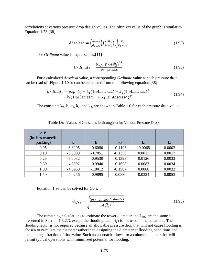
1-75
correlations at various pressure drop design values. The Abscissa value of the graph is similar to
Equation 1.73:[38]
𝐴𝑏𝑠𝑐𝑖𝑠𝑠𝑎 = (𝐿𝑚𝑜𝑙,𝑖
𝐺𝑚𝑜𝑙,𝑖) (
𝑀𝑊𝐿
𝑀𝑊𝐺) √
𝜌𝐺
𝑃𝐿−𝜌𝐺 (1.92)
The Ordinate value is expressed as:[11]
𝑂𝑟𝑑𝑖𝑛𝑎𝑡𝑒 =(𝐺𝑠𝑓𝑟,𝑖)
2𝐹𝑃(
𝜇𝐿2.42
)0.1
(𝜌𝐿−𝜌𝐺)𝜌𝐺𝑔𝑐 (1.93)
For a calculated Abscissa value, a corresponding Ordinate value at each pressure drop
can be read off Figure 1.10 or can be calculated from the following equation:[38]
𝑂𝑟𝑑𝑖𝑛𝑎𝑡𝑒 = 𝑒𝑥𝑝[ 𝑘0 + 𝑘1(1𝑛𝐴𝑏𝑠𝑐𝑖𝑠𝑠𝑎) + 𝑘2(1𝑛𝐴𝑏𝑠𝑐𝑖𝑠𝑠𝑎)2
+𝑘3(1𝑛𝐴𝑏𝑠𝑐𝑖𝑠𝑠𝑎)3 + 𝑘4(1𝑛𝐴𝑏𝑠𝑐𝑖𝑠𝑠𝑎)4] (1.94)
The constants k0, kl, k2, k3, and k4, are shown in Table 1.6 for each pressure drop value.
Table 1.6: Values of Constants k0 through k4 for Various Pressure Drops
∆ P
(inches water/ft
packing) k0 k1 k2 k3 k4
0.05 -6.3205 -0.6080 -0.1193 -0.0068 0.0003
0.10 -5.5009 -0.7851 -0.1350 0.0013 0.0017
0.25 -5.0032 -0.9530 -0.1393 0.0126 0.0033
0.50 -4.3992 -0.9940 -0.1698 0.0087 0.0034
1.00 -4.0950 -1.0012 -0.1587 0.0080 0.0032
1.50 -4.0256 -0.9895 -0.0830 0.0324 0.0053
Equation 1.93 can be solved for Gsfr,i.
𝐺𝑠𝑓𝑟,𝑖 = √(𝜌𝐿−𝜌𝐺)𝜌𝐺𝑔𝑐(𝑂𝑟𝑑𝑖𝑛𝑎𝑡𝑒)
𝐹𝑃(𝜇𝐿
2.42)
0.1 (1.95)
The remaining calculations to estimate the tower diameter and Lsfr,i are the same as
presented in Section 1.3.2.3, except the flooding factor (f) is not used in the equations. The
flooding factor is not required because an allowable pressure drop that will not cause flooding is
chosen to calculate the diameter rather than designing the diameter at flooding conditions and
then taking a fraction of that value. Such an approach allows for a column diameter that will
permit typical operations with minimized potential for flooding.

1-76
Figure 1.11: Generalized Pressure Drop Correlations [38]
Figure 1.12: Packed Tower Equipment Cost [44]
1.3.3 Estimating Total Capital Investment
This section presents the procedures and data necessary for estimating capital costs for
vertical packed bed gas absorbers using countercurrent flow to remove gaseous pollutants from

1-77
waste gas streams. Equipment costs for packed bed absorbers are presented in Section 1.3.3.1,
with installation costs presented in Section 1.3.3.2.
Total capital investment, TCI, includes equipment cost, EC, for the entire gas absorber
unit, taxes, freight charges, instrumentation, and direct and indirect installation costs. All costs
are presented in third quarter 1991 dollars. For escalating these and the other scrubber costs to
more current year dollars, the EPA suggests that the Chemical Engineering Plant Cost Index
(CEPCI) could be useful. This cost index covers construction and equipment costs for the
chemical process industries, a likely sector for installation of these control devices. The CEPCI is
available at http://www.chemengonline.com/pci.14
As for the rest of this chapter and the Control Cost Manual, the costs presented are study
estimates with an expected accuracy of ± 30 percent. It must be kept in mind that even for a
given application, design and manufacturing procedures vary from vendor to vendor, so costs
vary. All of these costs are for new plant installations; no retrofit cost considerations are
included.
1.3.3.1 Equipment Costs for Packed Tower Absorbers
Gas absorber vendors were asked to supply cost estimates for a range of tower
dimensions (i.e., height, diameter) to account for the varying needs of different applications. The
equipment for which they were asked to provide costs consisted of a packed tower absorber
made of fiberglass reinforced plastic (FRP), and to include the following equipment components:
• absorption column shell;
• gas inlet and outlet ports;
• liquid inlet port and outlet port/drain;
• liquid distributor and redistributor;
• two packing support plates;
• mist eliminator;
• internal piping;
• sump space; and
• platforms and ladders.
The cost data the vendors supplied were first adjusted to put them on a common basis,
and then were regressed against the absorber surface area (S). The equation shown below is a
linear regression of cost data provided by six vendors in 1991 dollars. [40, 44]
𝑇𝑜𝑡𝑎𝑙𝑇𝑜𝑤𝑒𝑟𝐶𝑜𝑠𝑡($) = 115 × 𝑆 (1.96)
where S is the surface area of the absorber, in ft2. Figure 1.11 depicts a plot of Equation 1.96.
This equation is applicable for towers with surface areas from 69 to 1,507 ft2 constructed of FRP.
14 Please note that mention of the Chemical Engineering Plant Cost Index (CEPCI) in this Manual is not meant to
serve as endorsement for commercial purposes. In addition, escalation of costs beyond 5 years is typically not
recommended according to Section 1, Chapter 2 (Cost Estimation Methodology) of this Control Cost Manual. We
escalated these costs from 1991 to 2016 costs given insufficient control cost data in more recent year dollars.
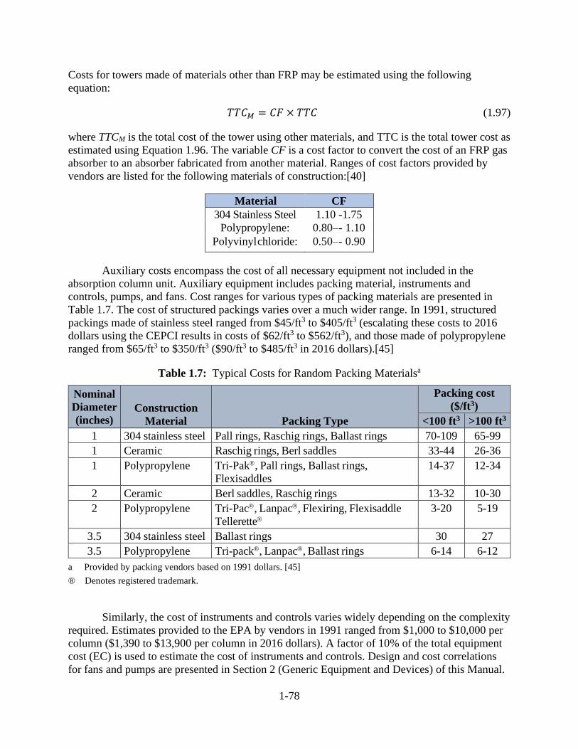
1-78
Costs for towers made of materials other than FRP may be estimated using the following
equation:
𝑇𝑇𝐶𝑀 = 𝐶𝐹 × 𝑇𝑇𝐶 (1.97)
where TTCM is the total cost of the tower using other materials, and TTC is the total tower cost as
estimated using Equation 1.96. The variable CF is a cost factor to convert the cost of an FRP gas
absorber to an absorber fabricated from another material. Ranges of cost factors provided by
vendors are listed for the following materials of construction:[40]
Material CF
304 Stainless Steel 1.10 -1.75
Polypropylene: 0.80–- 1.10
Polyvinylchloride: 0.50–- 0.90
Auxiliary costs encompass the cost of all necessary equipment not included in the
absorption column unit. Auxiliary equipment includes packing material, instruments and
controls, pumps, and fans. Cost ranges for various types of packing materials are presented in
Table 1.7. The cost of structured packings varies over a much wider range. In 1991, structured
packings made of stainless steel ranged from $45/ft3 to $405/ft3 (escalating these costs to 2016
dollars using the CEPCI results in costs of $62/ft3 to $562/ft3), and those made of polypropylene
ranged from $65/ft3 to $350/ft3 ($90/ft3 to $485/ft3 in 2016 dollars).[45]
Table 1.7: Typical Costs for Random Packing Materialsa
Nominal
Diameter
(inches) Construction
Material Packing Type
Packing cost
($/ft3)
<100 ft3 >100 ft3
1 304 stainless steel Pall rings, Raschig rings, Ballast rings 70-109 65-99
1 Ceramic Raschig rings, Berl saddles 33-44 26-36
1 Polypropylene Tri-Pak, Pall rings, Ballast rings,
Flexisaddles
14-37 12-34
2 Ceramic Berl saddles, Raschig rings 13-32 10-30
2 Polypropylene Tri-Pac, Lanpac, Flexiring, Flexisaddle
Tellerette
3-20 5-19
3.5 304 stainless steel Ballast rings 30 27
3.5 Polypropylene Tri-pack, Lanpac, Ballast rings 6-14 6-12
a Provided by packing vendors based on 1991 dollars. [45]
® Denotes registered trademark.
Similarly, the cost of instruments and controls varies widely depending on the complexity
required. Estimates provided to the EPA by vendors in 1991 ranged from $1,000 to $10,000 per
column ($1,390 to $13,900 per column in 2016 dollars). A factor of 10% of the total equipment
cost (EC) is used to estimate the cost of instruments and controls. Design and cost correlations
for fans and pumps are presented in Section 2 (Generic Equipment and Devices) of this Manual.

1-79
However, cost data for auxiliary equipment are also available from the literature (e.g., see
reference 45).
The EC is the sum of the component equipment costs, which includes costs for the tower,
packing material and the auxiliary equipment.
𝐸𝐶 = 𝑇𝑇𝐶 + 𝑃𝑎𝑐𝑘𝑖𝑛𝑔𝐶𝑜𝑠𝑡 + 𝐴𝑢𝑥𝑖𝑙𝑖𝑎𝑟𝑦𝐸𝑞𝑢𝑖𝑝𝑚𝑒𝑛𝑡 (1.98)
The purchased equipment cost (PEC) includes the cost of the absorber with packing and
its auxiliaries (EC), instrumentation (0.10 EC), sales tax (0.03 EC), and freight (0.05 EC): [40,
47],
𝑃𝐸𝐶 = (1 + 0.10 + 0.03 + 0.05)𝐸𝐶 = 1.18𝐸𝐶 (1.99)
1.3.3.2 Installation Costs
As discussed in Section 1, Chapter 2 of this Manual, the TCI is estimated from the total
purchased equipment cost via direct and indirect installation cost factors and a contingency
factor. A breakdown of the factors for wet packed tower absorbers is shown in Table 1.8. [47]
The installation factors presented in Table 1.8 were confirmed by the absorber vendors. [40]
As indicated in Section 1.2, Chapter 2 of this Manual, the TCI also includes costs for
land, working capital, and off-site facilities, which are not included in the direct/indirect
installation factor. However, as these items are rarely required with wet scrubbers, they will not
be included in the TCI here. Further, no factors have been provided for site preparation (SP) and
buildings (Bldg.), as these site-specific costs depend very little on the purchased equipment cost.
Thus, the total capital investment, TCI, is obtained by multiplying the purchased
equipment cost, PEC, by the total installation factor and adding an amount for contingencies:
𝑇𝐶𝐼 = 2.17 × 𝑃𝐸𝐶 + 𝐶 (1.100)
The contingency, C, accounts for unexpected costs associated with the fabrication and
installation of the absorber and is calculated by multiplying the total direct and indirect costs by a
contingency factor (CF). A default value of 10% of the direct and indirect costs is typically used
for CF. However, values of between 5% and 15% may be used. More information can be found
on contingency in Section 1, Chapter 2 of this Manual.
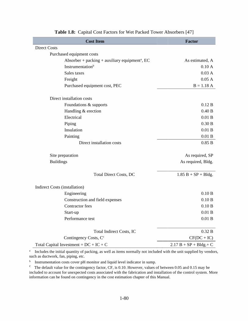
1-80
Table 1.8: Capital Cost Factors for Wet Packed Tower Absorbers [47]
Cost Item Factor
Direct Costs
Purchased equipment costs
Absorber + packing + auxiliary equipmenta, EC As estimated, A
Instrumentationb 0.10 A
Sales taxes 0.03 A
Freight 0.05 A
Purchased equipment cost, PEC B = 1.18 A
Direct installation costs
Foundations & supports 0.12 B
Handling & erection 0.40 B
Electrical 0.01 B
Piping 0.30 B
Insulation 0.01 B
Painting 0.01 B
Direct installation costs 0.85 B
Site preparation As required, SP
Buildings As required, Bldg.
Total Direct Costs, DC 1.85 B + SP + Bldg.
Indirect Costs (installation)
Engineering 0.10 B
Construction and field expenses 0.10 B
Contractor fees 0.10 B
Start-up 0.01 B
Performance test 0.01 B
Total Indirect Costs, IC 0.32 B
Contingency Costs, Cc CF(DC + IC)
Total Capital Investment = DC + IC + C 2.17 B + SP + Bldg.+ C
a Includes the initial quantity of packing, as well as items normally not included with the unit supplied by vendors,
such as ductwork, fan, piping, etc. b Instrumentation costs cover pH monitor and liquid level indicator in sump. c The default value for the contingency factor, CF, is 0.10. However, values of between 0.05 and 0.15 may be
included to account for unexpected costs associated with the fabrication and installation of the control system. More
information can be found on contingency in the cost estimation chapter of this Manual.

1-81
1.3.4 Estimating Annual Cost for Wet Packed Tower Absorbers
The total annual cost (TAC) is the sum of the direct and indirect annual costs.
1.3.4.1 Direct Annual Costs
Direct annual costs (DAC) are those expenditures related to operating the equipment,
such as labor and materials. The suggested factors for each of these costs are shown in Table 1.9.
Table 1.9: Suggested Annual Cost Factors for Wet Packed Tower Absorbers
Cost Item Factor
Direct Annual Costs, DAC
Operating labora
Operator 0.5 hour per shift
Supervisor 15% of operator labor
Operating materialsb Application specific
Solvent (throughput/yr) x (waste fraction)
Chemicals Based on annual consumption
Wastewater disposal (throughput/yr) x (waste fraction)
Maintenancea
Labor 0.5 hour per shift
Material 100% of maintenance labor
Electricity (consumption rate) x (hours/yr) x (unit cost)
Fan
Pump
Indirect Annual Costs, IAC
Overhead 60% of total labor and material costs
Administrative charges 2% of Total Capital Investment
Property tax 1% of Total Capital Investment
Insurance 1% of Total Capital Investment
Capital recoveryc 0.0527 x Total Capital Investment
Total Annual Cost DAC + IAC
a These factors were confirmed by vendor contacts. b If system does not use chemicals (e.g., caustic), this quantity is equal to annual solvent consumption. c Assuming a 30-year life at 3.25%. See Chapter 2.

1-82
These factors were taken from Section 1 of this Manual and were confirmed by absorber
vendors. The annual cost for each item is calculated by multiplying the number of units used
annually (i.e., hours, pounds, gallons, kWh) by the associated unit cost.
Operating labor is estimated at 0.5-hour per 8-hour shift. The supervisory labor cost is
estimated at 15% of the operating labor cost. Maintenance labor is estimated at 0.5-hour per 8-
hour shift. Maintenance materials costs are assumed to equal maintenance labor costs.
Solvent costs are dependent on the total liquid throughput, the type of solvent required,
and the fraction of solvent throughput wasted (often referred to as blow-down). Typically, the
fraction of solvent wasted varies from 0.1% to 10% of the total solvent throughput.[40] For acid
gas absorbers, the amount of solvent wasted is determined by the solids content, with bleed off
occurring when solids content reaches 10% to 15% to prevent salt carry-over.[40]
The total annual cost of solvent (Cs) is given by:
𝐶𝑠 = 𝐿𝑖𝑊𝐹 ((60𝑚𝑖𝑛
ℎ𝑟) (
𝑎𝑛𝑛𝑢𝑎𝑙𝑜𝑝𝑒𝑟𝑎𝑡𝑖𝑛𝑔
ℎ𝑜𝑢𝑟𝑠
) (𝑠𝑜𝑙𝑣𝑒𝑛𝑡
𝑢𝑛𝑖𝑡 𝑐𝑜𝑠 𝑡)) (1.101)
where WF is the waste (make-up) fraction, and the solvent unit cost is expressed in terms of
$/gal.
The cost of chemical replacement (Cc) is based on the annual consumption of the
chemical and can be calculated by:
𝐶𝑐 = (𝑙𝑏𝑠𝑐ℎ𝑒𝑚𝑖𝑐𝑎𝑙𝑢𝑠𝑒𝑑
ℎ𝑟) (
𝑎𝑛𝑛𝑢𝑎𝑙𝑜𝑝𝑒𝑟𝑎𝑡𝑖𝑛𝑔
ℎ𝑜𝑢𝑟𝑠
) (𝑐ℎ𝑒𝑚𝑖𝑐𝑎𝑙𝑢𝑛𝑖𝑡 𝑐𝑜𝑠 𝑡
) (1.102)
where the chemical unit cost is in terms of $/lb.
Solvent disposal (Cww) costs vary depending on geographic location, type of waste
disposed of, and availability of on-site treatment. Solvent disposal costs are calculated by:
𝐶𝑤𝑤 = 𝐿𝑖𝑊𝐹 (60𝑚𝑖𝑛
ℎ𝑟) (
𝑎𝑛𝑛𝑢𝑎𝑙𝑜𝑝𝑒𝑟𝑎𝑡𝑖𝑛𝑔
ℎ𝑜𝑢𝑟𝑠
) (𝑠𝑜𝑙𝑣𝑒𝑛𝑡
𝑑𝑖𝑠𝑝𝑜𝑠𝑎𝑙 𝑐𝑜𝑠 𝑡) (1.103)
where the solvent disposal costs are in terms of $/gal of waste solvent.
The electricity costs associated with operating a gas absorber derive from fan
requirements to overcome the pressure drop in the column, ductwork, and other parts of the
control system, and pump requirements to recirculate the solvent. The energy required for the fan
can be calculated using Equation 1.104:
𝐸𝑛𝑒𝑟𝑔𝑦𝑓𝑎𝑛 =1.17×10⁻⁴𝐺𝑖𝐷𝑃
𝜀 (1.104)

1-83
where Energy (in kilowatts) refers to the energy needed to move a given volumetric flow rate of
air (acfm), Gi is the waste gas flow rate entering the absorber, P is the total pressure drop through
the system (inches of H2O) and D is the combined fan-motor efficiency. Values for D typically
range from 0.4 to 0.7. Likewise, the electricity required by a recycle pump can be calculated
using Equation 1.105:
𝐸𝑛𝑒𝑟𝑔𝑦𝑝𝑢𝑚𝑝 =(0.746)(2.52×10⁻⁴)𝐿𝑖(𝑝𝑟𝑒𝑠𝑠𝑢𝑟𝑒)
𝜀 (1.105)
where 0.746 is the factor used to convert horsepower to kW, pressure is expressed in feet of
water, and Ԑ is the combined pump-motor efficiency.
The cost of electricity (Ce) is then given by:
𝐶𝑒 = 𝐸𝑛𝑒𝑟𝑔𝑦𝑓𝑎𝑛+𝑝𝑢𝑚𝑝 (𝑎𝑛𝑛𝑢𝑎𝑙
𝑜𝑝𝑒𝑟𝑎𝑡𝑖𝑛𝑔ℎ𝑜𝑢𝑟𝑠
) (𝑐𝑜𝑠 𝑡 𝑜𝑓
𝑒𝑙𝑒𝑐𝑡𝑟𝑖𝑐𝑖𝑡𝑦) (1.106)
where cost of electricity is expressed in units of $/kW-hr.
1.3.4.2 Indirect Annual Costs
Indirect annual costs (IAC) include overhead, taxes, insurance, general and
administrative (G&A), and capital recovery costs. The suggested factors for each of these items
are shown in Table 1.9. Overhead is assumed to be equal to 60% of the sum of operating,
supervisory, maintenance labor and maintenance materials. Overhead cost is discussed in Section
1, Chapter 2 of this Manual.
The system capital recovery cost, CRC, is based on an estimated 30-year equipment life,
which is consistent with the estimate used for wet and dry FGD systems stated earlier in this
chapter.15 For a 30-year equipment life and an interest rate of 3.25%, the capital recovery factor
(CF) is 0.0527. The system capital recovery cost is then estimated by:
𝐶𝑅𝐶 = 0.0527 × 𝑇𝐶𝐼 (1.107)
G&A costs, property tax, and insurance are factored from the total capital investment
(TCI), typically at 2%, 1%, and 1%, respectively.
1.3.4.3 Total Annual Cost
Total annual cost (TAC) is calculated by adding the direct annual costs and the indirect
annual costs.
𝑇𝐴𝐶 = 𝐷𝐴𝐶 + 𝐼𝐴𝐶 (1.108)
15 See Section 1, Chapter 2 of this Control Cost Manual for a discussion of the capital recovery cost.

1-84
1.3.4.4 Cost Effectiveness
The cost in dollars per ton of pollutant removed per year, is calculated as follows:
𝐶𝑜𝑠𝑡 𝐸𝑓𝑓𝑒𝑐𝑡𝑖𝑣𝑒𝑛𝑒𝑠𝑠 =𝑇𝐴𝐶
𝑃𝑜𝑙𝑙𝑢𝑡𝑎𝑛𝑡 𝑅𝑒𝑚𝑜𝑣𝑒𝑑(𝑡𝑜𝑛𝑠/𝑦𝑟) (1.109)
Where:
Cost Effectiveness = the cost effectiveness, $/ton
SO2 Removed/yr = annual mass of SO2 removed by the absorber, ton/yr
TAC = total annual cost, $/year
1.3.5 Example Problem for a Wet Packed Tower Absorber
The example problem presented in this section shows how to apply the sizing and costing
procedures presented in Sections 1.3.2 through 1.3.4 to design and cost wet tower absorber for
removing HCl from a waste gas stream consisting of HCl and air from an industrial process. This
example problem uses the same outlet stream parameters presented in example problem found in
Chapter 2 (Incinerators and Oxidizers) of this Manual for thermal and catalytic oxidizers. The
waste gas stream entering the gas absorber is assumed to be saturated with moisture due to being
cooled in the quench chamber. The concentration of HCl has also been adjusted to account for
the change in volume.
1.3.5.1 Determine the Waste Stream Characteristics
The first step in the design procedure is to specify the conditions of the gas stream to be
controlled and the desired pollutant removal efficiency. Gas and liquid stream parameters for this
example problem are listed in Table 1.10.
The quantity of HCl can be written in terms of lb-moles of HCl per lb-moles of pollutant-
free-gas (Yi) using the following calculation:
𝑌𝑖 =0.001871
1−0.001871= 0.00187
𝑙𝑏−𝑚𝑜𝑙𝑒𝑠𝐻𝐶𝑙
𝑙𝑏−molepollutantfreegas
The solvent, a dilute aqueous solution of caustic, is assumed to have the same physical
properties as water.
1.3.5.2 Determine Gas and Liquid Stream Properties
Once the properties of the waste gas stream entering the absorber are known, the
properties of the waste gas stream exiting the absorber and the liquid streams entering and
exiting the absorber need to be determined. The pollutant concentration in the entering liquid
(Xi) is assumed to be zero. The pollutant concentration in the exiting gas stream (Yo) is
calculated using Equation 1.57 and a removal efficiency of 99 percent.
𝑌𝑜 = 𝑌𝑖 (1 −𝜂
100) = 0.00187 (1 −
99
100) = 0.0000187

1-85
The liquid flow rate entering the column is calculated from the Ls/Gs ratio using Equation
1.58. Since Yi, Yo, and Xi are defined, the remaining unknown, Xo*, is determined by consulting
the equilibrium curve. A plot of the equilibrium curve-operating line graph for an HCl-water
system is presented in Figure 1.12. The value of Xo* is taken at the point on the equilibrium
curve where Yi intersects the curve. The value of Yi intersects the equilibrium curve at an X value
of 0.16.
Figure 1.13: Equilibrium Curve Operating Line for the HCl-Water System [8]

1-86
Table 1.10: Waste Stream Characteristics and Packing Properties for Example Problem
Parameters Values
Stream Properties
Waste Gas Flow Rate Entering Absorber 21,377 scfm (22,288 acfm)
Temperature of Waste Gas Stream 100°F
Pollutant in Waste Gas HCl
Concentration of HCl Entering Absorber in Waste Gas 1,871 ppmv
Pollutant Removal Efficiency 99% (molar basis)
Solvent Water with caustic in solution
Density of Waste Gasa 0.0709 lb/ft3
Density of Liquid [8] 62.4 lb/ft3
Molecular Weight of Waste Gasa 29 lb/lb-mole
Molecular Weight of Liquid [8] 18 lb/lb-mole
Viscosity of Waste Gasa 0.044 lb/ft-hr
Viscosity of Liquid [8] 2.16 lb/ft-hr
Minimum Wetting Rate [8] 1.3 ft2/hr
Pollutant Propertiesb
Diffusivity of HCl in Air 0.725 ft2/hr
Diffusivity of HCl in Water 1.02 x 10⁻⁴ ft2/hr
Packing Propertiesc
Packing type 2-inch ceramic Raschig rings
Packing factor: Fp 65
Packing constant: α 3.82
Packing constant: β 0.41
Packing constant: γ 0.45
Packing constant: φ 0.0125
Packing constant: b 0.22
Surface Area to Volume Ratio 28 a Reference [8], at 100oF b Appendix C. c Appendix B.

1-87
The operating line is constructed by connecting two points: (Xi, Yo) and (Xo*, Yi). The
slope of the operating line intersecting the equilibrium curve, (Ls/Gs)min, is:
(𝐿𝑠
𝐺𝑠)
𝑚𝑖𝑛
=𝑌𝑖 − 𝑌𝑜
𝑋𝑜∗ − 𝑋𝑖
=0.00187 − .0000187
0.16 − 0= 0.0116
The actual Ls/Gs ratio is calculated using Equation 1.60. For this example, an adjustment
factor of 1.5 will be used.
Gs =60ρ
GGi
MWG(1 + Yi)
𝐺𝑠 =
((60𝑚𝑖𝑛ℎ𝑟
) (0.0709𝑙𝑏
𝑓𝑡3) (22,288𝑎𝑐𝑓𝑚))
(29𝑙𝑏
𝑙𝑏 − 𝑚𝑜𝑙𝑒) (1 + 0.00187)
𝑙𝑏 − 𝑚𝑜𝑙𝑒𝑠ℎ𝑟
= 3,263 𝑙𝑏 − 𝑚𝑜𝑙𝑒𝑠
ℎ𝑟
The flow rate of the solvent entering the absorber may then be calculated using Equation
1.61.
𝐿𝑠 = (𝐿𝑠
𝐺𝑠)
𝑎𝑐𝑡
× 𝐺𝑠 = 0.0174 (3,263𝑙𝑏 − 𝑚𝑜𝑙𝑒𝑠
ℎ𝑟) = 56.8
𝑙𝑏 − 𝑚𝑜𝑙𝑒𝑠
ℎ𝑟
The values of Gmol,i and Lmol,i are calculated using Equations 1.62 and 1.63, respectively:
𝐺𝑚𝑜𝑙,𝑖 = 𝐺𝑠(1 + 𝑌𝑖) = (3,263𝑙𝑏 − 𝑚𝑜𝑙𝑒𝑠
ℎ𝑟) (1 + 0.00187) = 3,269
𝑙𝑏 − 𝑚𝑜𝑙𝑒𝑠
ℎ𝑟
𝐿𝑚𝑜𝑙,𝑖 = 𝐿𝑠(1 + 𝑋𝑖) = (56.8𝑙𝑏 − 𝑚𝑜𝑙𝑒𝑠
ℎ𝑟) (1 + 0) = 56.8
𝑙𝑏 − 𝑚𝑜𝑙𝑒𝑠
ℎ𝑟
The pollutant concentration existing the absorber in the liquid is calculated using
Equation 1.66.
𝑥𝑜 =𝑌𝑖 − 𝑌𝑜
(𝐿𝑠
𝐺𝑠)
+ 𝑋𝑖 =0.00187 − 0.0000187
0.0174=
0.106𝑙𝑏 − 𝑚𝑜𝑙𝑒𝑠𝐻𝐶𝑙
𝑙𝑏 − 𝑚𝑜𝑙𝑒𝑠𝑜𝑙𝑣𝑒𝑛𝑡
1.3.5.3 Calculate Absorption Factor
The absorption factor is calculated from the slope of the equilibrium line and the
Lmol,i/Gmol,i ratio. The slope of the equilibrium curve is based on the mole fractions of xi, xo, yi,
and yo, which are calculated from Xi, Xo, Yi and Yo* from Figure 1.12. From Figure 1.12, the
value of Yo* in equilibrium with the Xo value of 0.106 is 0.0001. The values of Yi and Xi are 0.
1-88
The mole fraction values are calculated from the concentration values using Equations 1.69
through 1.72.
𝑥𝑜 =0.106
1 + 0.106= 0.096
𝑦𝑜∗ =
0.0001
1 + 0.0001= 0.0001
The slope of the equilibrium fine from xi to xo is calculated from Equation 1.68:
m =yo
∗ −yi∗
xo−xi=
0.0001−0
0.096−0= 0.00104
Since HCl is very soluble in water, the slope of the equilibrium curve is very small. The
absorption factor is calculated from Equation 1.67.
AF =Lmol,i
mGmol,i=
0.0174
0.00104= 17
1.3.5.4 Estimate Column Diameter
Once the inlet and outlet stream conditions are determined, the diameter of the gas
absorber may be calculated using the modified generalized pressure drop correlation presented in
Figure 1.9. The Abscissa value from the graph is calculated from Equation 1.73:
𝐴𝑏𝑠𝑐𝑖𝑠𝑠𝑎 = (𝐿𝑚𝑜𝑙,𝑖
𝐺𝑚𝑜𝑙,𝑖) (
𝑀𝑊𝐿
𝑀𝑊𝐺) √
𝜌𝐺
𝜌𝐿
𝐴𝑏𝑠𝑐𝑖𝑠𝑠𝑎 = 0.0174 (18
29) √
0.0709
62.4= 0.000364
Since this value is outside the range of Figure 1.9, the smallest value (0.01) will be used as a
default value. The Ordinate is calculated from Equation 1.75.
𝑂𝑟𝑑𝑖𝑛𝑎𝑡𝑒 = 10[−1.668−1.085(𝑙𝑜𝑔 𝐴𝑏𝑠𝑐𝑖𝑠𝑠𝑎)−0.297(𝑙𝑜𝑔 𝐴𝑏𝑠𝑐𝑖𝑠𝑠𝑎)2]
𝑂𝑟𝑑𝑖𝑛𝑎𝑡𝑒 = 10[−1.668−1.085(𝑙𝑜𝑔 0.01)−0.297(𝑙𝑜𝑔 0.01)2] = 0.207
The superficial gas flow rate, Gsfr,i, is calculated using Equation 1.74. For this example
calculation, 2-inch ceramic Raschig rings are selected as the packing. The packing factors for
Raschig rings are listed in Appendix B.
1-89
Gsfr,i = √ρ
l ρ
G gc (Ordinate)
Fp Ψ (μ
L
2.42)0.2
𝐺𝑠𝑓𝑟,𝑖 =√
(0.207)(62.4) (0.0709𝑙𝑏
𝑓𝑡3) (32.2𝑓𝑡
𝑠𝑒𝑐2)
(65)(1)(0.893)0.2= 0.681
𝑙𝑏
𝑠𝑒𝑐 − 𝑓𝑡2
Once Gsfr,i is determined, the cross-sectional area of the column is calculated using
Equation 1.77.
𝐴 =𝐺𝑚𝑜𝑙,𝑖 𝑀𝑊𝐺
3,600 𝐺𝑠𝑓𝑟,𝑖𝑓=
(3,263𝑙𝑏 − 𝑚𝑜𝑙
ℎ𝑟) (29
𝑙𝑏𝑙𝑏 − 𝑚𝑜𝑙
)
((3,600𝑠𝑒𝑐ℎ𝑟
) (0.681𝑙𝑏
𝑠𝑒𝑐 − 𝑓𝑡2) (0.7))
2 = 55.1 𝑓𝑡2
The superficial liquid flow rate is determined using Equation 1.79.
𝐿𝑠𝑓𝑟,𝑖 =𝐿𝑚𝑜𝑙,𝑖 𝑀𝑊𝐿
𝐴=
(56.8𝑙𝑏 − 𝑚𝑜𝑙
ℎ𝑟) (18
𝑙𝑏𝑙𝑏 − 𝑚𝑜𝑙
)
55.1𝑓𝑡2= 18.6
𝑙𝑏
ℎ𝑟 − 𝑓𝑡2
At this point, it is necessary to determine if the liquid flow rate is sufficient to wet the
packed bed. The minimum value of Lsfr,i is calculated using Equation 1.80. The packing constant,
a, is found in Appendix B, Table B-1.
(𝐿𝑠𝑓𝑟,𝑖)𝑚𝑖𝑛= 𝑀𝑊𝑅𝜌𝐿𝑎 = (1.3
𝑓𝑡2
ℎ𝑟) (62.4
𝑙𝑏
𝑓𝑡3) (28
𝑓𝑡2
𝑓𝑡3) = 2,271
𝑙𝑏
ℎ𝑟 − 𝑓𝑡2
The Lsfr,i value calculated using the L/G ratio is far below the minimum value needed to wet the
packed bed. Therefore, the new value, (Lsfr,i)min will be used to determine the diameter of the
absorber. The calculations for this revised diameter are shown in Appendix D. Appendix D
shows that the cross-sectional area of the column is calculated to be 60 ft2, Lmol,i is 7572 lb-
mole/hr, and Gsfr,i is 0.627 lb/sec-ft2. The diameter of the column is then calculated using
Equation 1.78:
𝐷 = √(4)(60𝑓𝑡)2
𝜋= 8.74𝑓𝑡
The value of Xo is then:
𝑥𝑜 =0.00187−0.0000187
7,572
3,263
= 0.0008

1-90
Expressed in terms of mole fraction:
𝑥𝑜 =0.0008
1 − 0.0008= 0.0008
The value of yo in equilibrium with xo cannot be estimated accurately. However, the value will
approach zero, and the value of AF will be extremely large:
𝐴𝐹 =7,572
(3,263)(≈ 0)→ ∞
1.3.5.5 Calculate Column Surface Area
Since xi = 0 and AF is large, Equation 1.82 will be used to calculate the number of
transfer units:
Ntu =In [(
yi − mxi
yo − mxi) (1 −
1AF) +
1AF]
1 −1
AF
= 𝑙𝑛 (0.00187
0.0000187) = 4.61
The height of a transfer unit is calculated from, AF, HL, and HG. The values of HG and HL are
calculated from Equations 1.87 and 1.88:
HG = [α(3,600fGsfr,i)
β
(Lsfr,i)Γ] √
μG
ρG
DG(
μLΓ
μG
β)
𝐻𝐺 =3.82[(3,600)(0.7)(0.627)]0.41
2,2710.45√
0.044
(0.725)(0.0709)= 2.24𝑓𝑡
𝐻𝐿 = 𝜙 (𝐿𝑠𝑓𝑟,𝑖
𝜇𝐿)
𝑏
√𝜇𝐿
𝜌𝐿𝐷𝐿(
𝑇
286)
−4.255
𝐻𝐿 = 0.0125 (2,271
2.16)
0.22
√2.16
(0.000102)(62.4)= 1.06𝑓𝑡
The height of the transfer unit is calculated using Equation 1.84:
𝐻𝑡𝑢 = 𝐻𝐺 +1
𝐴𝐹 𝐻𝐿 = (2.24𝑓𝑡) +
1
∞(1.06𝑓𝑡) = 2.24𝑓𝑡
The depth of packing is calculated from Equation 1.81.
1-91
𝐻𝑝𝑎𝑐𝑘 = 𝑁𝑡𝑢 × 𝐻𝑡𝑢 = (4.61 × 2.24𝑓𝑡) = 10.3𝑓𝑡
The total height of the column is calculated from Equation 1.89:
𝐻𝑡𝑜𝑤𝑒𝑟 = 1.4𝐻𝑝𝑎𝑐𝑘 + 1.02𝐷 + 2.81 = 1.40(10.3) + 1.02(8.74) + 2.81 = 26.1𝑓𝑡
The surface area of the column is calculated using Equation 1.90:
𝑠 = 𝜋𝐷 (𝐻𝑡𝑜𝑤𝑒𝑟 + 𝐷
2) = (3.14)(8.74) (26.1 +
8.74
2) = 836𝑓𝑡2
1.3.5.6 Calculate Pressure Drop
The pressure drop through the column is calculated using Equation 1.91.
ΔP = c 10(
j Lsfr,i3,600
) (fGsfr,i)2
ρG
𝛥𝑃 = (0.24)10(
(0.17)(2,271)3,600
) [(0.7)(0.627)]
0.0709
2
= 0.83 inches water/foot packing
The total pressure drop (through 10.3 feet of packing) equals 8.55 inches of water.
1.3.5.7 Equipment Costs
Once the system sizing parameters have been determined, the equipment costs can be
calculated. For this example, a gas absorber constructed of FRP will have its equipment costs
estimated using Equation 1.97. The cost is converted to the current year dollars using the
Chemical Engineering Plant Cost Index (CEPCI). In this example, the scaling factor for 2016
dollars is 541.7/390.6.16
𝑇𝑇𝐶($) = 115𝑆 × [𝐶𝐸𝑃𝐶𝐼2016
390.6] = 115(836) × [
541.7
390.6] = $133,331
The cost of 2-inch ceramic Raschig rings can be estimated from packing cost ranges
presented in Section 1.3.5. The volume of packing required is calculated as:
𝑉𝑜𝑙𝑢𝑚𝑒 𝑜𝑓𝑝𝑎𝑐𝑘𝑖𝑛𝑔 = (60𝑓𝑡2)(10.3𝑓𝑡) = 618𝑓𝑡3
16 Escalation of the equipment costs from 1991 dollars to 2016 dollars is not typically recommended according to
Section 1, Chapter 2 of this Manual. For purposes of the example, however, we have escalated the costs since we do
not have more recent equipment costs currently available. If they are available and documented, more recent
equipment costs are preferred for cost estimates as they avoid escalation beyond five years, as mentioned in Chapter
1, Section 2 of the Control Cost Manual.

1-92
Using the average of the cost range for 2-inch ceramic packings, the total cost of packing
is:
𝑃𝑎𝑐𝑘𝑖𝑛𝑔 𝑐𝑜𝑠 𝑡 = (618𝑓𝑡3)($20/𝑓𝑡3) (541.7
390.6) = $17,141
For this example problem, the cost of a pump will be estimated using vendor quotes.
First, the flow rate of solvent must be converted into units of gallons per minute:
𝐿(𝑔𝑝𝑚) = (2,271𝑙𝑏
ℎ − 𝑓𝑡2) (60𝑓𝑡2) (
𝑔𝑎𝑙
8.34𝑙𝑏) (
ℎ𝑟
60𝑚𝑖𝑛) = 272 𝑔𝑝𝑚
The average price for an FRP pump of this size is $22.2/gpm at a pressure of 60 ft water,
based on information from vendors ($16/gpm in 1991 dollars escalated to 2016 dollars using
CEPCI).[40] Therefore, the cost of the recycle pump is estimated as:
𝐶𝑝𝑢𝑚𝑝 = (272𝑔𝑝𝑚) ($22.2
𝑔𝑝𝑚) = $6,038
For this example, the cost for a fan (FRP, backwardly-inclined centrifugal) can be
calculated using the following equation:[46]
𝐶𝑓𝑎𝑛 = 57.9𝑑1.38 × [541.7
390.6]
where d is the impeller (wheel) diameter of the fan expressed in inches. For this gas flow rate
and pressure drop, an impeller diameter of 33 inches is needed. At this diameter, the cost of the
fan is:
𝐶𝑓𝑎𝑛 = 57.9(33)1.38 × [541.7
390.6] = $10,006
The cost of a fan motor (three-phase, carbon steel) with V-belt drive, belt guard, and
motor starter can be computed as follows:[46]
𝐶𝑚𝑜𝑡𝑜𝑟 = 104(ℎ𝑝)0.821 × [547.1
390.6]
As will be shown in Section 1.3.5.8, the electricity consumption of the fan is 32.0 kW.
Converting to horsepower, we obtain a motor size of 42.6 hp. The cost of the fan motor is:
𝐶𝑚𝑜𝑡𝑜𝑟 = 104(42.6)0.821 × [541.7
390.6] = $3,139
The total auxiliary equipment cost is:
$6,038 + $10,006+ $3,139 = $19,183
1-93
The total equipment cost in 2016 dollars is the sum of the absorber cost, the packing cost,
and the auxiliary equipment cost:
EC = TTC + Packing Cost + Auxiliary Equipment = 133,331 + 17,141 + 19,183 = $169,655
The purchased equipment cost including instrumentation, controls, taxes, and freight is
estimated using Equation 1.99:
PEC = 1.18 EC= 1.18(169,655) = $200,193
The total capital investment is calculated using Equation 1.100 and using a contingency
factor of 10%:
TCI = 2.17PEC + C =2.17(200,193) + (0.1)(2.17)(200,193) = $477,861
1.3.5.8 Total Annual Cost
Table 1.11 summarizes the estimated annual costs using the suggested factors and unit
costs for the example problem.
Direct annual costs for gas absorber systems include labor, materials, utilities, and
wastewater disposal. Labor costs are based on 8,000 hr/yr of operation. Supervisory labor is
computed at 15% of operating labor and operating and maintenance labor are each based on 0.5
hr per 8-hr shift.
The electricity required to run the fan is calculated using Equation 1.104 and assuming a
combined fan-motor efficiency of 70%:
Energyfan =1.17 × 10⁻⁴GiDP
ε=
(1.17 × 10⁻⁴)(22,288)(8.55)
0.70= 32.0 𝑘𝑊
The energy required for the liquid pump is calculated using Equation 1.105. The capital
cost of the pump was calculated using data supplied by vendors for a pump operating at a
pressure of 60 feet of water. Assuming a pressure of 60 ft of water a combined pump-motor
efficiency of 70 percent:
𝐸𝑛𝑒𝑟𝑔𝑦𝑝𝑢𝑚𝑝 =(0.746)(2.52 × 10⁻⁴)𝐿𝑖(𝑝𝑟𝑒𝑠𝑠𝑢𝑟𝑒)
ɛ=
(0.746)(2.52 × 10⁻⁴)(272)(60)(1)
0.70= 4.4 𝑘𝑤
The total energy required to operate the auxiliary equipment is approximately 36.4 kW.
The cost of electricity, Ce, is calculated using Equation 1.106 and with the cost per kWh shown
in Table 1.11.
𝐶𝑒 = (𝐸𝑛𝑒𝑟𝑔𝑦𝑓𝑎𝑛 + 𝐸𝑛𝑒𝑟𝑔𝑦𝑝𝑢𝑚𝑝)(𝑂𝑝𝑒𝑟𝑎𝑡𝑖𝑛𝑔 𝐻𝑜𝑢𝑟𝑠)(𝐶𝑜𝑠𝑡 𝑜𝑓 𝐸𝑙𝑒𝑐𝑡𝑟𝑖𝑐𝑡𝑦)
= (36.4𝑘𝑊)(8,000ℎ/𝑦𝑟)($0.0674/𝑘𝑊ℎ) = $19,627/𝑦𝑟

1-94
The costs of solvent (water), wastewater disposal, and caustic are all dependent on the
total system throughput and the fraction of solvent discharged as waste. A certain amount of
solvent will be wasted and replaced by a fresh solution of water and caustic in order to maintain
the system’s pH and solids content at acceptable levels. Based on data provided by vendors, a
maximum solids content of 10% by weight will be the design basis for this example
problem.[46] The following calculations illustrate the procedure used to calculate how much
water and caustic are needed, and how much solvent must be bled off to maintain system
operability.
From previous calculations, Lmol,i = 7,572 lb-moles/hr. The mass flow rate is calculated
as:
𝐿𝑚𝑎𝑠𝑠 = (7,572𝑙𝑏 − 𝑚𝑜𝑙𝑒
ℎ𝑟) (18
𝑙𝑏
𝑙𝑏 − 𝑚𝑜𝑙𝑒) = 136,296
𝑙𝑏
ℎ𝑟
With Gmol,i at 3,263 lb-moles/hr, the mass flow rate of the gas stream is calculated as:
𝐺𝑚𝑎𝑠𝑠 = (3,263𝑙𝑏 − 𝑚𝑜𝑙𝑒
ℎ𝑟) (29
𝑙𝑏
𝑙𝑏 − 𝑚𝑜𝑙𝑒) = 94,627
𝑙𝑏
ℎ𝑟
The amount of HCl in the gas stream is calculated on a molar basis as follows:
𝐺𝑚𝑎𝑠𝑠 = (3,263𝑙𝑏 − 𝑚𝑜𝑙𝑒
ℎ𝑟) (1,874
𝑝𝑝𝑚𝑣
1 × 10⁶) = 6.11
𝑙𝑏 − 𝑚𝑜𝑙𝐻𝐶𝑙
ℎ𝑟
On a mass basis:
𝐺𝑚𝑎𝑠𝑠,𝐻𝐶𝑙 = (6.11𝑙𝑏 − 𝑚𝑜𝑙𝐻𝐶𝐿
ℎ𝑟) (36.5
𝑙𝑏
𝑙𝑏 − 𝑚𝑜𝑙𝑒) = 223.0
𝑙𝑏𝐻𝐶𝑙
ℎ𝑟
For this example, the caustic is assumed to be Na2O, with one mole of caustic required
for neutralizing 2 moles of HCl. Therefore, 3.06 lb-moles/hr of caustic are required.
The unit cost of a 76% solution of Na2O is given in Table 1.11. The annual cost is
calculated from:
𝐶𝑐 = (3.06𝑙𝑏−𝑚𝑜𝑙𝑒𝑠
ℎ𝑟) (62
𝑙𝑏
𝑙𝑏−𝑚𝑜𝑙𝑒) (
8,000ℎ𝑟
𝑦𝑟) (
𝑡𝑜𝑛
2,000𝑙𝑏) (
1
0.76) (
$340
𝑡𝑜𝑛) = $339,499/𝑦𝑒𝑎𝑟
Mass of the salt formed in this chemical reaction, sodium chloride (NaC1), is calculated
as:
𝑀𝑎𝑠𝑠𝑁𝑎𝐶𝑙 = (223.0𝑙𝑏 − 𝐻𝐶𝑙
ℎ𝑟) (
𝑙𝑏 − 𝑚𝑜𝑙𝑒
36.5𝑙𝑏𝐻𝐶𝑙) (
1𝑙𝑏 − 𝑚𝑜𝑙𝑒𝑁𝑎𝐶𝑙
𝑙𝑏 − 𝑚𝑜𝑙𝑒𝐻𝐶𝑙) (
58.5𝑙𝑏𝑁𝑎𝐶𝑙
𝑙𝑏 − 𝑚𝑜𝑙𝑒𝑁𝑎𝐶𝑙)
= 357.4𝑙𝑏 𝑁𝑎𝐶𝑙/ℎ𝑜𝑢𝑟

1-95
If the maximum concentration of NaC1 in the wastewater (ww) is assumed to be 10
weight %, the wastewater volume flow rate is calculated as:
gpm
hr
wwlb
wwgal
NaCllb
wwlb
hr
NaCllbWastewaterflowrate
14.7
min60
1
34.81.0
14.357
=
=
Where 8.34 is the density of the wastewater.
The cost of wastewater disposal is:17
𝐶𝑤𝑤 = (7.14𝑔𝑝𝑚) (60𝑚𝑖𝑛
ℎ𝑟) (
8,000ℎ𝑟𝑠
𝑦𝑟) (
$5.70
1,000𝑔𝑎𝑙) = $19,535
The cost of solvent (water) is:
𝐶𝑠 = (7.14𝑔𝑝𝑚) ((60𝑚𝑖𝑛
1ℎ𝑟) (8,000
ℎ𝑟
𝑦𝑟) (
$4.20
1,000𝑔𝑎𝑙)) =
$14,394
𝑦𝑒𝑎𝑟
Indirect annual costs include overhead, administrative charges, property tax, insurance,
and capital recovery. Total annual cost is estimated using Equation 1.108. For this example, the
total annual cost is estimated to be $516,000 per year (Table 1.11).
Table 1.11: Annual Costs for Packed Tower Absorber Example Problem
Cost Item Calculations Cost
Direct Annual Costs, DAC
Operating Labor
Operator(a) 0.5ℎ𝑟
𝑠ℎ𝑖𝑓𝑡×
𝑠ℎ𝑖𝑓𝑡
8ℎ𝑟×
8,000ℎ𝑟
𝑦𝑟×
$26.61
ℎ𝑟 $13,305
Supervisor 15% 𝑜𝑓 𝑜𝑝𝑒𝑟𝑎𝑡𝑜𝑟 = 0.15 × 13,305 $1,996
Operating materials
Solvent (water)(b) 7.14𝑔𝑝𝑚 ×60 𝑚𝑖𝑛
ℎ𝑟×
8,000 ℎ𝑟
𝑦𝑟×
$4.20
1,000 𝑔𝑎𝑙 $14,394
17 Because the wastewater stream contains only NaC1, it probably will not require pretreatment before discharge to a
municipal wastewater treatment facility. Therefore, the wastewater disposal unit cost shown here is just a sewer
usage rate. This unit cost ($5.25/1,000 gal) is the average sewer rates for industrial facilities in 2013 compiled by
Black & Veatch. See “50 Largest Cities Water/Wastewater Rate Survey.” Available at
http://www.saws.org/who_we_are/community/RAC/docs/2014/50-largest-cities-brochure-water-wastewater-rate-
survey.pdf.

1-96
Cost Item Calculations Cost
Caustic
Replacement(c)
3.06 𝑙𝑏 − 𝑚𝑜𝑙𝑒
ℎ𝑟×
62 𝑙𝑏
𝑙𝑏 − 𝑚𝑜𝑙𝑒×
8,000 ℎ𝑟
𝑦𝑟×
𝑡𝑜𝑛
2,000 𝑙𝑏
×1
0.76×
$340
𝑡𝑜𝑛
$339,499
Wastewater
disposal(b) 7.14 𝑔𝑝𝑚 (
60 𝑚𝑖𝑛
ℎ𝑟) (
8,000 ℎ𝑟
𝑦𝑟) (
$5.70
1,000 𝑔𝑎𝑙) $19,535
Maintenance
Labor(d) 0.5
𝑠ℎ𝑖𝑓𝑡× (
𝑠ℎ𝑖𝑓𝑡
8 ℎ𝑟) × (
8,000 ℎ𝑟
𝑦𝑟) × ($29.27/ℎ𝑜𝑢𝑟) $14,635
Material 100% of maintenance labor $14,635
Electricity(e) 36.4 𝑘𝑤 ×8,000 ℎ𝑟
𝑦𝑟×
$0.0676
𝑘𝑊ℎ $19,685
Total DAC $437,684
Indirect Annual Costs, IAC(f)
Overhead 60% of total labor and maintenance material:
= 0.6(13,305 + 1,996 + 14,635 + 14,635) $27,943
Administrative
charges 2% of Total Capital Investment = 0.02 ($477,861) $9,557
Property tax 1% of Total Capital Investment = 0.01 ($477,861) $4,779
Insurance 1% of Total Capital Investment = 0.01 ($477,861) $4,779
Capital recovery(g) 0.0527 x $477,861 $25,183
Total IAC $72,241
Total Annual Cost
(rounded) DAC + IAC $509,925
(a) Bureau of Labor Statistics, May 2016 National Occupational Employment and Wage Estimates – United States,
May 2016 (https://www.bls.gov/oes/2016/may/oes_nat.htm). Hourly rates for operators based on data for Plant and
System Operators – other (51-8099). (b) Average water rates for industrial facilities in 2016 compiled by Black & Veatch. See “50 Largest Cities
Water/Wastewater Rate Survey – 2018-2019.” Available at https://www.bv.com/sites/default/files/2019-
10/50_Largest_Cities_Rate_Survey_2018_2019_Report.pdf. (c) Price of caustic soda based on July 2016 data reported in Outlook ’17: The Calm Before the Storm for European
Caustic Soda, ICIS, January 11, 2017 (available at
https://www.icis.com/explore/resources/news/2017/01/11/10064199/outlook-17-the-calm-before-the-storm-for-
european-caustic-soda/). (d) Maintenance labor rate is estimated at 110% of the operator wage rate. (e) U.S. Energy Information Administration. Electric Power Annual 2016. Table 2.10. Published December 2017.
Available at: https://www.eia.gov/electricity/annual/pdf/epa.pdf. (f) Indirect annual costs include overhead, administrative charges, property tax, insurance, and capital recovery.
Total annual cost is estimated using Equation 1.108. (g) The capital recovery cost factor, CRF, is a function of the absorber equipment life and the opportunity cost of
the capital (i.e., interest rate). For this example, we assume a 30-year equipment life and a 3.25% interest rate.

1-97
1.3.5.9 Cost Effectiveness
The cost in dollars per ton of pollutant removed per year, is calculated as follows:
𝐶𝑜𝑠𝑡 𝐸𝑓𝑓𝑒𝑐𝑡𝑖𝑣𝑒𝑛𝑒𝑠𝑠 =𝑇𝐴𝐶
𝐻𝐶𝑙𝑅𝑒𝑚𝑜𝑣𝑒𝑑/𝑦𝑒𝑎𝑟=
$509,925/𝑦𝑒𝑎𝑟
894𝑡𝑜𝑛𝑠/𝑦𝑒𝑎𝑟= $570/𝑡𝑜𝑛
1.3.5.10 Alternate Example
In this example problem the diameter of a gas absorber will be estimated by defining a
pressure drop. A pressure drop of 1 inch of water per foot of packing will be used in this example
calculation. Equation 1.94 is used to calculate the ordinate value relating to an abscissa value. If
the Lmole,i/Gmol,i ratio is known, the Abscissa can be calculated directly. The Ordinate value is:
Ordinate = exp[ k0 + k1(1nAbscissa) + k2(1nAbscissa)2
+k3(1nAbscissa)3 + k4(1nAbscissa)4]
𝑂𝑟𝑑𝑖𝑛𝑎𝑡𝑒 = 𝑒𝑥𝑝[ − 4.0950 − 1.00121𝑛(0.0496) − 0.1587(1𝑛0.0496)2 +
0.0080(1𝑛0.0496)3 + 0.0032(1𝑛0.0496)4]= 0.084
The value of Gsfr is calculated using Equation 1.95:
Gsfr,i = √(ρ
L− ρ
G)ρ
Ggc(Ordinate)
FP (μ
L
2.42)0.1
𝐺𝑠𝑓𝑟,𝑖 = √(62.4 − 0.0709)(0.0709)(32.2)(0.084)
65(0.893)0.1= 0.43
𝑙𝑏
𝑓𝑡2 − 𝑠𝑒𝑐
The remaining calculations are the same as in Section 1.3.5.4, except the flooding factor is not
used in the equations.

1-98
Acknowledgments
The authors gratefully acknowledge the following companies and organizations for
contributing data to this chapter:
• Air Plastics, Inc. (Cincinnati, OH)
• April, Inc. (Teterboro, NJ)
• Anderson 2000, Inc. (Peachtree City, GA)
• Calvert Environmental (San Diego, CA)
• Ceilcote Air Pollution Control (Berea, OH)
• Croll-Reynolds Company, Inc. (Westfield, NJ)
• Ecolotreat Process Equipment (Toledo, OH)
• Glitsch, Inc. (Dallas, TX)
• Institute of Clean Air Companies (ICAC) (Arlington, VA)
• Interel Corporation (Englewood, CO)
• Jaeger Products, Inc. (Spring, TX)
• Koch Engineering Co., Inc. (Wichita, KS)
• Lantec Products, Inc. (Agoura Hills, CA)
• Midwest Air Products Co., Inc. (Owosso, MI)
• Monroe Environmental Corp., (Monroe, MI)
• Norton Chemical Process Products (Akron, OH)

1-99
References
[1] U.S. EPA, Control Technologies for Hazardous Air Pollutants, Office of Research and
Development, U.S. Environmental Protection Agency, Research Triangle Park, North
Carolina, Publication No. EPA 625/6-91-014, 1991.
[2] McInnes, R., K. Jameson, and D. Austin, Scrubbing Toxic Inorganics, Chemical
Engineering, September 1990, pp. 116-121.
[3] U.S. EPA, Air Pollution Control Technology Fact Sheet – Flue Gas Desulfurization,
U.S. EPA, EPA-452/F-03-034, Washington, D.C. 2002.
(https://www3.epa.gov/ttn/catc/dir1/ffdg.pdf)
[4] Letter from S. Raymond Woll of Air Products, Inc., to William M. Vatavuk, U.S.
Environmental Protection Agency, June 25, 1992.
[5] Letter from Jose L. Bravo of Jaeger Products, Inc., to William M. Vatavuk, U. S.
Environmental Protection Agency, June 8, 1992.
[6] Letter from Jack D. Brady of Anderson 2000, Inc., to William M. Vatavuk, U.S.
Environmental Protection Agency, June 9, 1992.
[7] Treybal, Robert E., Mass Transfer Operations (Third edition), McGraw-Hill Book
Company, New York, 1980.
[8] Perry, R.H. and C.H. Chilton, Eds., Chemical Engineers’ Handbook (Sixth edition),
McGraw-Hill Book Company, New York, 1984.
[9] United States of America v. Ameren Missouri, No. 4:11-cv-00077-RWS (E.D. Mo.
Sept. 30, 2019).18
[10] Vatavuk, William M., Estimating Costs of Air Pollution Control, Lewis Publishers,
1990, p. 198.
[11] Warych, J. and M. Szymanowski, Optimum Values of Process Parameters of the Wet
Limestone Flue Gas Desulfurization System, Chemical Engineering & Technology, v.
25, 2002, pp. 427-432.
[12] EPA, Technical Support Document for the Oklahoma Regional Haze State
Implementation Plan and Federal Implementation Plan. March 2011.
18 The case is currently on appeal before the U.S. Circuit Court of Appeals for the Eighth Circuit. United States v.
Ameren Missouri, No. 19-3220 (8th Cir. argued Dec. 16, 2020), however, the emission rates, control efficiencies,
and cost data provided in the opinion are accurate and are not at issue in the appeal.

1-100
[13] U.S. EPA, Technical Support Document for the Cost of Controls for the Texas
Regional Haze Federal Implementation Plan, November 2014.
[14] U.S. EPA, Srivastava, Ravi K. Controlling SO2 Emissions: A Review of Technologies,
U.S. EPA, Office of Research and Development. EPA/600/R-00/093, Washington,
D.C. 2000, available for download at
https://cfpub.epa.gov/si/si_public_record_report.cfm?dirEntryId=18978&Lab=NRMR
L.
[15] Cordoba, P., Status of Flue Gas Desulfurization (FGD) Systems from Coal-fired Power
Plants: Overview of the Physic-Chemical Control Processes of Wet Limestone, Fuel,
144, 2015.
[16] US EPA, Clean Air Markets Program Data, Coal-fired Characteristics and Controls:
2019, available at https://www.epa.gov/airmarkets/power-plant-data-highlights.
[17] Sargent & Lundy, LLC, Flue Gas Desulfurization Technology Evaluation Dry Lime vs.
Wet Limestone FGD, March 2007, available for download at
https://www.lime.org/documents/publications/free_downloads/fgdte_dry-wet-
limestone2007.pdf.
[18] Department of Energy, Energy Information Administration, Annual Electric Generator
Report (EIA-860) Data Files for 2018, available for download at
https://www.eia.gov/electricity/data/eia860/.
[19] US EPA, Clean Air Markets Program Data, Unit Level Emissions Data:2000 through
2018, available at https://ampd.epa.gov/ampd/.
[20] U.S. EPA, Documentation for the Integrated Planning Model – Updates to Cost and
Performance for APC Technologies, SDA FGD Cost Methodology, version 6, U.S.
EPA, Clean Air Markets, January 2017.
[21] U.S. EPA, Documentation for the Integrated Planning Model – Updates to Cost and
Performance for APC Technologies, Wet FGD Cost Methodology, version 6, U.S.
EPA, Clean Air Markets, January 2017.
[22] National Aeronautics and Space Administration (NASA), Earth Atmosphere Model.
Available at https://spaceflightsystems.grc.nasa.gov/education/rocket/atmos.html.
[23] U.S. EPA, Steam Electric Power Generation in Point Source Category: Final Detailed
Study Report, EPA 821-R-09-008, Oct 2009,
https://www.epa.gov/sites/production/files/2015-06/documents/steam-
electric_detailed_study_report_2009.pdf.
[24] Brad Buecker, Scrubbing: Optimizing Flue Gas Desulfurization Technologies Is
Essential, Power Magazine, September 1, 2006.

1-101
[25] Benson, L.B., K.J. Smith, and R.A. Roden, Control of Sulfur Dioxide and Sulfur Trioxide
Using By-Product of Magnesium-Enhanced Lime FGD System, IAC Forum: Multi-
Pollutant Emission Controls and Strategies, 2003.
[26] Schnelle, K.B. Jr and Brown, C.A. Air Pollution Control Technology Handbook, CRC
Press LLC. Boca Raton, Florida, 2002.
[27] Frey, Elaine F. 2013, Technology Diffusion and Environmental Regulation: The
Adoption of Scrubbers by Coal-Fired Power Plants, The Energy Journal 34(1): 177-
205.
[28] Shoemaker, L.E., and J.R. Crum, Experience in Effective Application of Metallic
Materials for Construction of FGD Systems, Special Metals Corporation, available at
http://pccforgedproducts.com/web/user_content/files/wyman/Metallic%20Materials%20f
or%20Construction%20of%20FGD%20Systems.pdf.
[29] Dille, E., K. Frizzell, and W. Shim, Use of an Electrochemical Technique for Controlling
Corrosion in FGD Reaction Tanks, EPRI-DOE-EPA Combined Utility Air Pollution
Control Symposium: The Mega Symposium: Volume 1: SO2 Controls, EPRI, Palo Alto,
CA, 1999.
[30] Correspondence from D. Shepherd, National Park Service, Air Resources Division to L.
Sorrels, US EPA, June 2020.
[31] Institute of Clean Air Companies (ICAC), Acid Gas/SO2 Controls,
https://www.icac.com/page/Acid_Gas_SO2_Control, accessed October 15, 2019.
[32] Correspondence from D. Shepherd, National Park Service, Air Resources Division to
L. Sorrels, US EPA, regarding 2018 and 2019 SO2 emissions for TS Power Plant,
Eureka County, Nevada, January 2020.
[33] Babcock & Wilcox product literature, available at https://www.babcock.com/-
/media/documents/products/cds/pch-605-lansing-cds.ashx, accessed February 12,
2020.
[34] ServoTech Industries, product literature, available at
http://servotechco.com/img/servotech-images/pdfs/products/2-ServoTech-
Circulating%20Dry%20Scrubber.pdf, accessed February 12, 2020.
[35] LDX Solutions, product literature, available at
https://www.ldxsolutions.com/technologies/circulating-dry-scrubber-cds/, accessed
February 12, 2020.
[36] Crowe, Charles R., and D. Cooper, Brick/Membrane Linings Pass the Acid Test, Chemical
Engineering, July 1988, pp. 83-86.
1-102
[37] Harrison, Mark E., and John J. France, Distillation Column Troubleshooting, Part 2:
Packed Columns, Chemical Engineering, April 1989, pp. 121-128.
[38] Coker, A.K., Understanding the Basics of Packed-Column Design, Chemical
Engineering Progress, November 1991, pp. 93-99.
[39] Telephone conversation between Roy Oommen, Radian Corporation and Gerald Nealon,
Norton Process Equipment, April 4, 1992.
[40] Gas absorber questionnaire responses from nine gas absorber vendors to Radian
Corporation, August-December, 1991.
[41] Buonicore, A.J., and L. Theodore, Industrial Control Equipment for Gaseous
Pollutants, Volume I, CRC Press, Inc., Cleveland, Ohio, 1975.
[42] Strigle, Ralph F., Random Packings and Packed Towers, Design Applications, Gulf
Publishing Company, Houston, Texas, 1987.
[43] Questionnaire response from K.C. Lang of Lantec Products, Inc. To R.V. Oommen,
Radian Corporation, August 23, 1991.
[44] Memorandum from Vatavuk, W.M. of U.S. Environmental Protection Agency to Martha
Smith, U.S. EPA, March 27, 1992.
[45] Packing vendor questionnaire responses from seven packing vendors to Radian
Corporation– August 1991 - January 1992.
[46] Vatavuk, W.M., Pricing Equipment for Air-Pollution Control, Chemical Engineering,
May 1990, pp. 126-130.
[47] Vatavuk, W.M., and R.B. Neveril, Estimating Costs of Pollution Control Systems, Part II:
Factors for Estimating Capital and Operating Costs, Chemical Engineering, November
3, 1980, pp. 157-162.
[48] Air Pollution Engineering Manual (AP-40), (Second Edition), Danielson, John A., Los
Angeles County Air Pollution Control District, CA, May 1973.
[49] U.S. EPA, Technical Development Document for the Effluent Limitations Guidelines
and Standards for the Steam Electric Power Generating Point Source Category, Office
of Water, EPA-821-R-15-007, September 2015, available for download at
https://www.epa.gov/sites/production/files/2015-10/documents/steam-electric-tdd_10-
21-15.pdf.
[50] U.S. EPA, Control of Mercury Emissions from Coal-fired Electric Utility Boilers,
Office of Research and Development, available for download at
https://www3.epa.gov/airtoxics/utility/hgwhitepaperfinal.pdf#:~:text=Control%20of%
20mercury%20emissions%20from%20coal-

1-103
fired%20boilers%20is,2%2Bcompounds%20in%20wet%20flue%20gas%20desulfuriz
ation%20%28FGD%29%20systems.
[51] U.S. EPA, Supplemental Technical Development Document for Proposed Revisions to
the Effluent Limitations Guidelines and Standards for the Steam Electric Power
Generating Point Source Category, Office of Water, EPA-821-R-19-009, November
2019, available for download at https://www.epa.gov/sites/production/files/2019-
11/documents/steam-electric-proposed-suppl-tdd_nov-2019.pdf.
[52] Cichanowicz, J.E., Capital Cost and Cost-Effectiveness of Electric Utility Coal-Fired
Power Plant Emissions Control Technologies: 2017Update, Utility Air Regulatory
Group, December 2017.
[53] Cichanowicz, J.E and M.C. Hein, Technical Comments on the Draft EPA Air Pollution
Control Cost Manual Chapter Wet Scrubbers for Acid Gas Control, November 3,
2020.
[54] Kelley, D., Resistant Fiberglass-reinforced Plastic for Wet FGD Applications, Power
Engineering, August 7, 2006 (available at https://www.power-eng.com/emissions/air-
pollution-control-equipment-services/resistant-fiberglass-reinforced-plastic-for-wet-
fgd-applications/#gref).
[55] Rapoza, R.J., H.R. Vollmer and K.L. Haberly, Guidelines for the use of Fiberglass
Reinforced Plastic in Utility Flue Gas Desulfurization Systems, Electric Power
Research Institute, TR-101654, November 1992 (available for download from
https://www.epri.com/research/products/TR-101654).
[56] EIA, More U.S. Coal-fired Power Plants are Decommissioning as Retirements
Continue, Today in Energy, July 26, 2019, (available at
https://www.eia.gov/todayinenergy/detail.php?id=40212).
[57] U.S. EPA, Supplemental Technical Development Document for Revisions to the Effluent
Limitations Guidelines and Standards for the Steam Electric Power Generating Point
Source Category, Office of Water, EPA-821-R-20-001, August 2020.
[58] U.S. EPA, Steam Electric Power Generating Point Source Category: Final Detailed
Study Report, Office of Water, EPA-821-R-09-008, October 2009.
[59] U.S. EPA, Technical Development Document for the Effluent Limitations Guidelines and
Standards for the Steam Electric Power Generating Point Source Category, Office of
Water, EPA-821-R-15-007, September 2015.
[60] Shell, product literature on the CANSOLV SO2 Scrubbing System, accessed at
https://www.shell.com/business-customers/catalysts-technologies/licensed-
technologies/emissions-standards/tail-gas-treatment-unit/cansolv.html.

1-104
[61] DuPont, product literature, accessed at
https://cleantechnologies.dupont.com/fileadmin/user_upload/Editor/CleanTechnologies/d
ocuments/41-_DuPont-MECS_SolvR_-Sulfuric-Acid.pdf.
[62] Ake, T. and A. Licata, Circulating Dry Scrubbers Comply with the EPA Maximum
Achievable Control Technology Limits, Babcock Power Technical Publication, 2011
(available at https://www.babcockpower.com/wp-content/uploads/2018/02/circulating-
dry-scrubbers-comply-with-the-epa-maximum-achievable-control-technology-
limits.pdf#:~:text=A%20Circulating%20Dry%20Scrubber%20is%20a%20pollution%20c
ontrol,or%20lime%20to%20react%20with%20flue%20gas%20constituents).
[63] Babcock Power, Circulating Dry Scrubbers, Webinar presentation at the 2012 Mid-
Atlantic Regional Air Management Association, July 2012 (available at
https://cdn.ymaws.com/www.icac.com/resource/resmgr/icac_regulatory_resources/babco
ck_power_cds_for_marma_.pdf).
[64] Buecker, B., Circulating Dry Scrubbers: A New Wave in FGD?, Power Engineering,
November 1, 2011. (available at https://www.power-eng.com/emissions/air-pollution-
control-equipment-services/circulating-dry-scrubbers-a-new-wave-in-fgd/).
[65] Kiang, Yen-Hsiung, Fuel Property Estimation and Combustion Process
Characterization, Academic Press 2018.
[66] AirPol product literature, accessed at https://irp-
cdn.multiscreensite.com/8ccf05af/files/uploaded/AirPol%20Acid%20Gas%20Absorption
%20Brochure.pdf.
[67] Envitech, product literature, accessed at
https://www.envitechinc.com/packed_bed_scrubbers.
[68] Gulf Coast Environmental Systems, product literature, available
http://www.gcesystems.com/dry-scrubber.html.
[69] Monroe Environmental, product literature, available at
https://www.monroeenvironmental.com/air-pollution-control/packed-bed-wet-scrubbers/.
[70] Babcock & Wilcox, product literature, available at
https://www.babcock.com/en/technology/pollution-control/so2-acid-gases.
[71] GE Power, product literature for wet FGD, available at
https://www.ge.com/power/steam/aqcs/sox-control-wfgd.
[72] GE Power, product literature for dry FGD systems, available at Dry Flue Gas
Desulfurization | SOx Control | GE Steam Power.
[73] Marsulex Environmental Technologies, product literature for dry FGD systems, available
at http://met.net/dry-fgd.aspx.

1-105
[74] LDX Solutions, product literature for wet scrubbers, available at
https://www.ldxsolutions.com/technologies/wet-scrubbers/.
[75] LDX Solutions, product literature for DustexTM Circulating Dry Scrubber (CDS),
available at https://www.ldxsolutions.com/circulating-dry-scrubber-cds/.

A-1
Appendix A
Table A-1: List of Design Variables For Wet FGD Systems
Variable Symbol Units Limestone consumption rate QLimestone tons/hour
Sulfur emission rate S lb/MMBtu
Unit size (gross) A MW
Heat rate factor HRF —
Removal efficiency EF fraction
Make-up water consumption rate qwater kgallons/hr
Coal factor CoalF —
Waste generation rate qwaste tons/hour
Electricity consumption P kW
Absorber island cost ABScost $
Reagent preparation cost RPEcost $
Waste handling equipment cost WHEcostl $
Balance of plant costs BOPcost $
Wastewater treatment plant cost WWTcost $
Retrofit factor RF —
Elevation factor ELEVF —
Number of hours of wastewater treatment top Hours/year
Capital recovery factor CRF —
Table A-2: List of Design Variables For Dry FGD Systems
Variable Symbol Units Lime consumption rate QLime tons/hour
Sulfur emission rate S lb/MMBtu
Unit size (gross) A MW
Heat rate factor HRF —
Removal efficiency EF fraction
Make-up water consumption rate qwater kgallons/hr
Coal factor CoalF —
Waste generation rate qww tons/hour
Electricity consumption P kW
Absorber island cost ABScost $
Balance of plant costs BOPcost $
Retrofit factor RF —
Elevation factor ELEVF —
Annual lime cost ARcost $
Number of operating hours top Hours/year
Capital recovery factor CRF —

A-2
Table A-3: List of Design Variables For Wet Packed Tower Absorbers
Variable Symbol Units
► Surface to volume ratio of packing a ft2/ft3
Cross-sectional area of absorber A ft2
Abscissa value from plot of generalized press drop correlation Abscissa —
Absorption factor AF —
Diameter of absorber D feet
► Diffusivity of pollutant in gas DG ft2/hr
► Diffusivity of pollutant in liquid DL ft2/hr
► Flooding factor f —
► Packing factor Fp —
► Waste gas flow rate entering absorber Gi acfm
Waste gas flow rate exiting absorber Go acfm
Waste gas molar flow rate entering absorber Gmol lb-moles/h
Molar flow rate of pollutant free gas Gs lb-moles/h
Waste gas superficial flow rate entering absorber Gsfr,i lb/sec-ft2
Height of gas transfer unit HG feet
Height of liquid transfer unit HL feet
Height of overall transfer unit Htu feet
Height of packing Hpack feet
Height of absorber Htower feet
Pressure drop constants k0, k1, k2, k3, k4 —
Liquid rate entering absorber Li gpm
Liquid rate exiting absorber Lo gpm
Liquid molar flow rate entering absorber Lmol,i lb-moles/h
Molar flow rate of pollutant free solvent Ls lb-moles/h
Liquid superficial flow rate entering absorber Lsfr,i lb/hr-ft2
Slope of equilibrium line m —
► Molecular weight of gas stream MWG lb/lb-mole
► Molecular weight of the liquid stream MWL lb/lb-mole
► Minimum wetting rate MWR ft2/hr
Number of overall transfer units Ntu —
Ordinate value from plot of generalized pressure drop correlation Ordinate —
Surface area of absorber S ft2
► Temperature of solvent T K
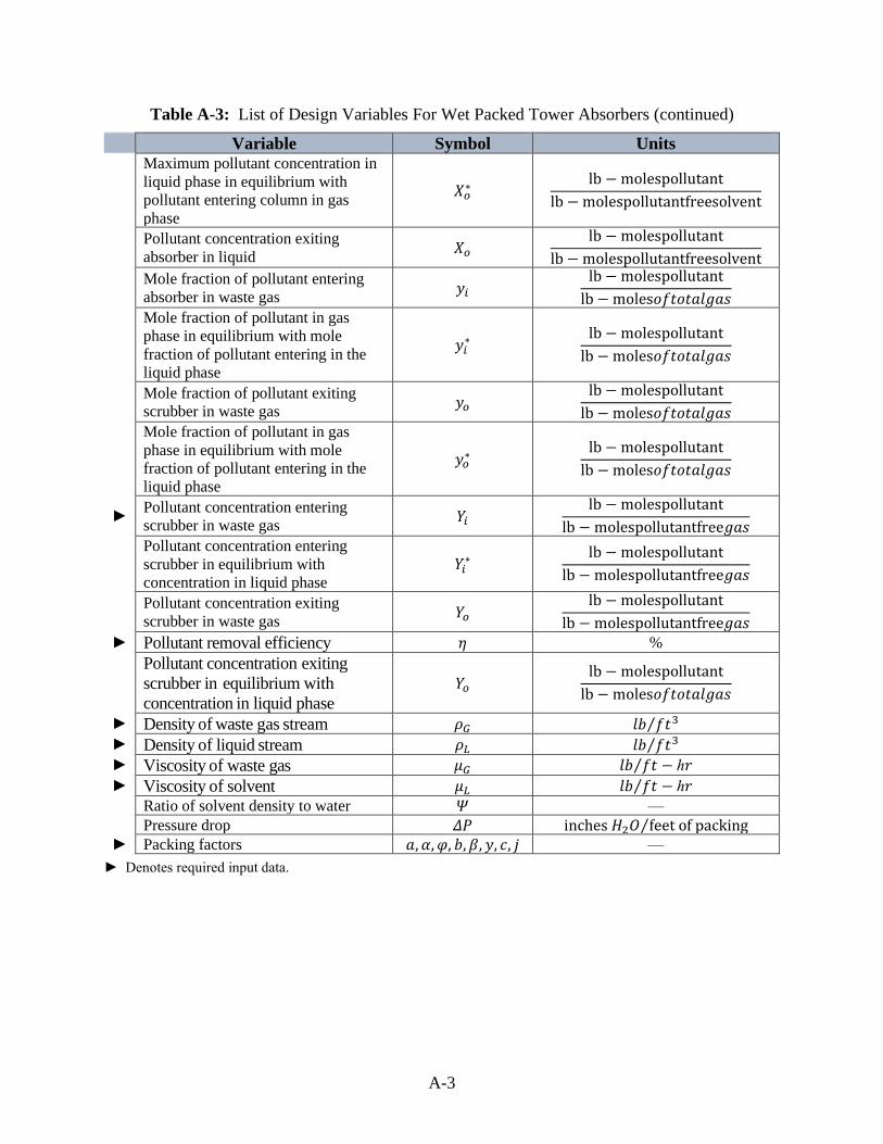
A-3
Table A-3: List of Design Variables For Wet Packed Tower Absorbers (continued)
Variable Symbol Units
Maximum pollutant concentration in
liquid phase in equilibrium with
pollutant entering column in gas
phase
𝑋𝑜∗
lb − molespollutant
lb − molespollutantfreesolvent
Pollutant concentration exiting
absorber in liquid 𝑋𝑜
lb − molespollutant
lb − molespollutantfreesolvent
Mole fraction of pollutant entering
absorber in waste gas 𝑦𝑖
lb − molespollutant
lb − moles𝑜𝑓𝑡𝑜𝑡𝑎𝑙𝑔𝑎𝑠
Mole fraction of pollutant in gas
phase in equilibrium with mole
fraction of pollutant entering in the
liquid phase
𝑦𝑖∗
lb − molespollutant
lb − moles𝑜𝑓𝑡𝑜𝑡𝑎𝑙𝑔𝑎𝑠
Mole fraction of pollutant exiting
scrubber in waste gas 𝑦𝑜
lb − molespollutant
lb − moles𝑜𝑓𝑡𝑜𝑡𝑎𝑙𝑔𝑎𝑠
Mole fraction of pollutant in gas
phase in equilibrium with mole
fraction of pollutant entering in the
liquid phase
𝑦𝑜∗
lb − molespollutant
lb − moles𝑜𝑓𝑡𝑜𝑡𝑎𝑙𝑔𝑎𝑠
► Pollutant concentration entering
scrubber in waste gas 𝑌𝑖
lb − molespollutant
lb − molespollutantfree𝑔𝑎𝑠
Pollutant concentration entering
scrubber in equilibrium with
concentration in liquid phase
𝑌𝑖∗
lb − molespollutant
lb − molespollutantfree𝑔𝑎𝑠
Pollutant concentration exiting
scrubber in waste gas 𝑌𝑜
lb − molespollutant
lb − molespollutantfree𝑔𝑎𝑠
► Pollutant removal efficiency 𝜂 %
Pollutant concentration exiting
scrubber in equilibrium with
concentration in liquid phase
𝑌𝑜 lb − molespollutant
lb − moles𝑜𝑓𝑡𝑜𝑡𝑎𝑙𝑔𝑎𝑠
► Density of waste gas stream 𝜌𝐺 𝑙𝑏 𝑓𝑡3⁄
► Density of liquid stream 𝜌𝐿 𝑙𝑏 𝑓𝑡3⁄
► Viscosity of waste gas 𝜇𝐺 𝑙𝑏 𝑓𝑡 − ℎ𝑟⁄
► Viscosity of solvent 𝜇𝐿 𝑙𝑏 𝑓𝑡 − ℎ𝑟⁄
Ratio of solvent density to water 𝛹 —
Pressure drop 𝛥𝑃 inches 𝐻2𝑂 feet of packing⁄
► Packing factors 𝑎, 𝛼, 𝜑, 𝑏, 𝛽, 𝑦, 𝑐, 𝑗 —
► Denotes required input data.

B-1
Appendix B
Table B-1: Packing Factors for Various Packing Materials for Wet Packed Tower Absorbers [5, 8, 38,
41]
Packing Type Construction Level
Nominal
Diameter
(inches) Fp a
Raschig rings Ceramic 1/2 640 111
5/8 380 100
3/4 255 80
1 160 58
1 ½ 95 38
2 65 28
3 37
Raschig rings Metal ½ 410 118
5/8 290
¾ 230 72
1 137 57
1 ½ 83 41
2 57 31
3 32 21
Pall rings Metal 5/8 70 131
1 48 66
1 ½ 28 48
2 20 36
3 1/2 16
Pall rings Polypropylene 58 97 110
1 52 63
1 ½ 32 39
2 25 31
Berl saddles Ceramic ½ 240 142
¾ 170 82
1 110 76
1 ½ 65 44
2 45 32
Intalox saddles Ceramic ½ 200 190
¾ 145 102
1 98 78
1 ½ 52 60
2 40 36
3 22
Tri-Packs® Plastic 2 16 48
3 ½ 12 38

B-2
Table B-2: Packing Constants Used to Estimate HG For Wet Packed Tower Absorbers [1, 5, 8,
41]
Packing Type
Size
(inches)
Packing Constants Applicable Rangea
α Β γ Gsfr Lsfr
Raschig Rings 3/8 2.32 0.45 0.47 200-500 500-1,500
1 7.00 0.39 0.58 200-800 400-500
1 6.41 0.32 0.51 200-600 500-4,500
1 1/2 1.73 0.38 0.66 200-700 500-1,500
1 1/2 2.58 0.38 0.40 200-700 1,500-4,500
2 3.82 0.41 0.45 200-800 500-4,500
Berl Saddles 1/2 32.4 0.30 0.74 200-700 500-1,500
1/2 0.81 0.30 0.24 200-700 1,500-4,500
1 1.97 0.36 0.40 200-800 400-4,500
1 1/2 5.05 0.32 0.45 200-1,000 400-4,500
Partition Rings 3 640 0.58 1.06 150-900 3,000-10,000
LanPac® 2.3 7.6 0.33 -0.48 400-3,000 500-8,000
Tri-Packs® 2 1.4 0.33 0.40 100-900 500-10,000
3 1/2 1.7 0.33 0.45 100-2,000 500-10,000 a Units of lb/hr-ft2
Table B-3: Packing Constants Used to Estimate HL For Wet Packed Tower Absorbers[1, 5, 41]
Packing Type Size (inches)
Packing Constants Applicable Rangea
φ b Lasfr
Raschig Rings 3/8 0.00182 0.46 400-15,000
1 0.00357 0.35 400-15,000
1 1/2 0.0100 0.22 400-15,000
2 1/2 0.0111 0.22 400-15,000
2 0.0125 0.22 400-15,000
Berl Saddles 1/2 0.00666 0.28 400-15,000
1 0.00588 0.28 400-15,000
1 1/2 0.00625 0.28 400-15,000
Partition Rings 3 0.0625 0.09 3,000-14,000
LanPac® 2.3 0.0039 0.33 500-8,000
3.5 0.0042 0.33 500-8,000
Tri-Packs® 2 0.0031 0.33 500-10,000
3 1/2 0.0040 0.33 500-10,000 a Units of lb/hr-ft2

B-3
Table B-4-: Packing Constants Used to Estimate Pressure Drop For Wet Packed Tower
Absorbers[1, 8, 41]
Packing Type
Construction
Material
Nominal
Diameter
(inches) c j
Raschig rings ceramic 1/2 3.1 0.41
3/4 1.34 0.26 1 0.97 0.25 1 ¼ 0.57 0.23 1 ½ 0.39 0.23 2 0.24 0.17 Raschig rings metal 5/8 1.2 0.28 1 0.42 0.21 11/2 0.29 0.20 2 0.23 0.135 Pall rings metal 5/8 0.43 0.17 1 0.15 0.16 11/2 0.08 0.15 2 0.06 0.12 Berl saddles ceramic 1/2 1.2 0.21
3/4 0.62 0.17 1 0.39 0.17 11/2 0.21 0.13 Intalox saddles ceramic 1/2 0.82 0.20 3/4 0.28 0.16 1 0.31 0.16 11/2 0.14 0.14
a Units of lb/hr-ft2
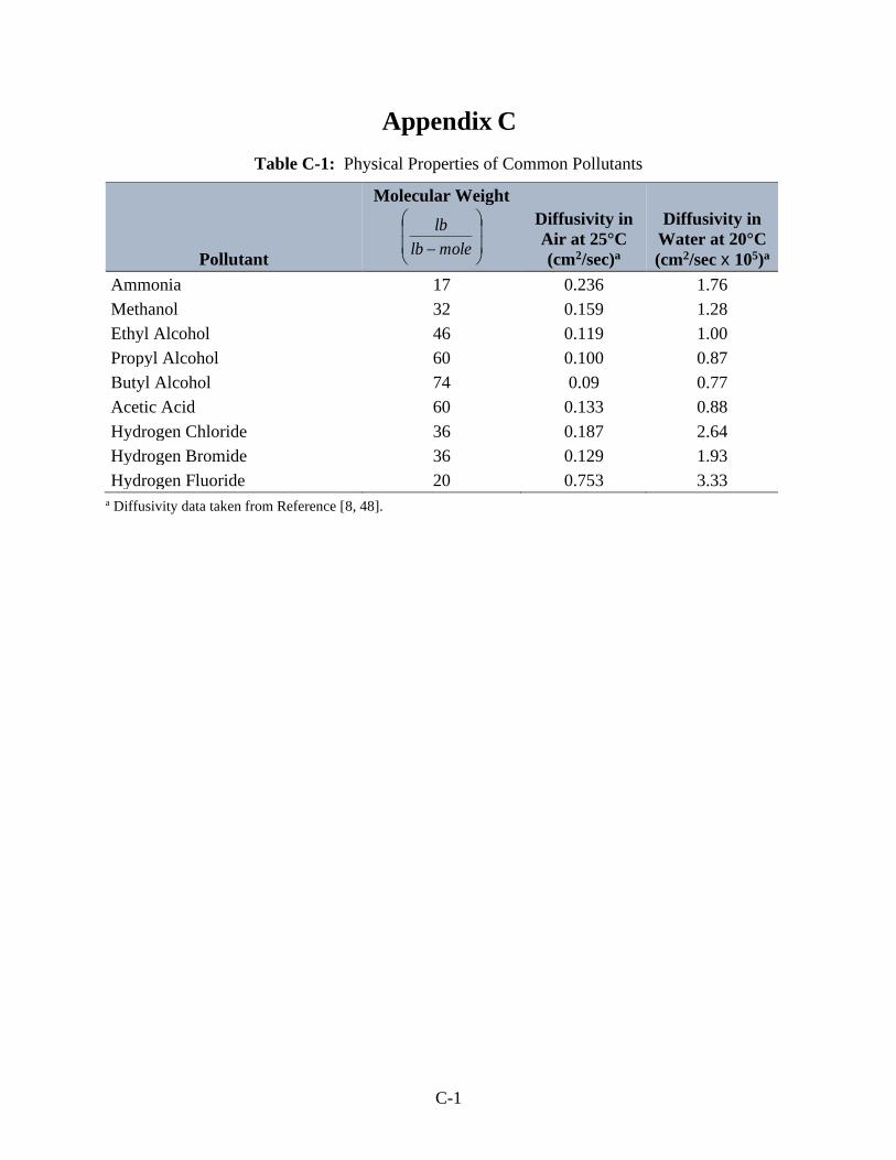
C-1
Appendix C
Table C-1: Physical Properties of Common Pollutants
Pollutant
Molecular Weight
− molelb
lb
Diffusivity in
Air at 25°C
(cm2/sec)a
Diffusivity in
Water at 20°C
(cm2/sec x 105)a
Ammonia 17 0.236 1.76
Methanol 32 0.159 1.28
Ethyl Alcohol 46 0.119 1.00
Propyl Alcohol 60 0.100 0.87
Butyl Alcohol 74 0.09 0.77
Acetic Acid 60 0.133 0.88
Hydrogen Chloride 36 0.187 2.64
Hydrogen Bromide 36 0.129 1.93
Hydrogen Fluoride 20 0.753 3.33 a Diffusivity data taken from Reference [8, 48].

D-1
Appendix D
Minimum Wetting Rate Analysis
As explained in the design procedures, the liquid flow rate entering the column must be
high enough to effectively wet the packing. If the liquid flow rate, as determined theoretically in
Equation 1.79, is lower than the flow rate dictated by the minimum wetting rate, calculated in
Equation 1.80, then the packing will not be wetted sufficiently to ensure mass transfer between
the gas and liquid phases. The minimum liquid flow rate should then be used as a default value.
The superficial gas flow rate, Gsfr, and cross-sectional area of the column must then be
recalculated to account for the increased liquid flow rate. The approach is outlined below:
• The value of Lmol,i must be recalculated from the value of (Lsfr,i)min using the equation:
𝐿𝑚𝑜𝑙,𝑖
(𝐿𝑠𝑓𝑟,𝑖)𝑚𝑖𝑛
(𝑀𝑊)𝐿 (D-1)
The value of A (the cross-sectional area of the absorber column) is the only unknown in the
equation.
• The Abscissa value is calculated in terms of A by substituting the new Lmol,i into Equation
1.73.
• The value of Gsfr,i is recalculated by rearranging Equation 1.77, with A as the only
unknown.
• The Ordinate value is calculated in terms of A from the new Gsfr,i using the Equation
1.74.
• An iterative process is used to determine A, Abscissa, and Ordinate. Values of A are
chosen and the Abscissa and Ordinate values are calculated. The Ordinate value
corresponding to the Abscissa value is determined from Figure 1.9 (or Equation 1.75),
and this value is compared to the Ordinate value calculated using Equation 1.74. This
process is continued until both Ordinate values are equal.
Step 1: The first step is to recalculate the liquid flow rate. The liquid molar flow rate may be
calculated using Equation 1.79.
𝐿𝑚𝑜𝑙,𝑖 = (2,271𝑙𝑏
ℎ𝑟−𝑓𝑡2) (𝑙𝑏−𝑚𝑜𝑙𝑒
18𝑙𝑏) 𝐴 = (126.2
𝑙𝑏−𝑚𝑜𝑙𝑒
ℎ𝑟−𝑓𝑡2 ) 𝐴 (D-2)

D-2
Step 2: The Abscissa value from Figure 1.9, and presented in Equation 1.73, is calculated as:
𝐴𝑏𝑠𝑐𝑖𝑠𝑠𝑎 =(126.2
𝑙𝑏−𝑚𝑜𝑙𝑒
ℎ𝑟−𝑓𝑡2 )𝐴
3,263𝑙𝑏−𝑚𝑜𝑙𝑒
ℎ𝑟
(18
29) √
0.0709
62.4 (D-3)
= 8.09𝑥10−4𝐴
Step 3: The value of Gsfr,i is then recalculated in terms of the cross-sectional area of the
column.
𝐺𝑠𝑓𝑟 =(3,263
𝑙𝑏−𝑚𝑜𝑙𝑒
ℎ𝑟−𝑓𝑡2 )(29𝑙𝑏
𝑙𝑏−𝑚𝑜𝑙𝑒)
(3,600𝑠𝑒𝑐
ℎ𝑟)(0.7)(𝐴)
=37.6
𝐴 (D-4)
Step 4: The ordinate value from Figure 1.9, and presented in Equation 1.74, is calculated as:
𝑂𝑟𝑑𝑖𝑛𝑎𝑡𝑒 =(
37.6
𝐴)
2(65)(1)(0.893)0.2
(62.4)(0.0709)(32.2) (D-5)
=631
𝐴2
Step 5: At this point the simplest solution is an iterative approach. Choose a value for A,
calculate the Abscissa value using Equation D-3, and find the corresponding Ordinate
value off the flooding curve in Figure 1.9 (or use Equation 1.75 to calculate the
Ordinate value). Compare the calculated Ordinate value from Equation D-5 to the
value obtained from the graph or from Equation 1.75. By continuing this process until
the Ordinate values converge the value of A is determined to be 60 ft2. The following
table illustrates the intermediate steps in the calculation process.
Table D-1: Results of Iterative Approach to Determining Column Cross-Sectional Area
Assumed Value of A
Abscissa Calculated
From Equation D-1
Ordinate Calculated
From Equation 9.81
Ordinate Calculated
From Equation D-2
65 0.0526 0.1714 0.1493
62 0.0503 0.1740 0.1642
60 0.0485 0.1757 0.1752

D-3
The value of Gsfr is then:
𝐺𝑠𝑓𝑟 =37.6
60= 0.627
𝑙𝑏
𝑠𝑒𝑐 − 𝑓𝑡2
The liquid molar flow rate is:
𝐿𝑚𝑜𝑙,𝑖 = (126.2)(60) = 7,572𝑙𝑏
𝑠𝑒𝑐 − 𝑓𝑡2
The diameter and height of the column using the results of this calculation are presented in the
example problem shown in Section 1.3.5.