ISO-NE PUBLIC Page 1 of 42

Section 1 Summary of Stability Base Cases for TPL 001-4 Studies This document accompanies the final base cases that have been posted to the ISO New England (ISO-NE) website under Planning Advisory Committee (PAC) materials1 on June 8, 2016 in order to coordinate with the PAC. The base cases will be utilized by ISO-NE to conduct studies needed to meet the NERC TPL-001-4 standard.

Any text adjacent to the blue square brackets ([R1]) in the sections below refers to a specific requirement in the NERC TPL 001-4 standard. If a subsection has such a designation then the information within that subsection pertains to the stated requirement in the standard.

The study base cases will cover the following:

1. Five year out peak load case (2021) to assess the near-term stability impact to meet requirement [R2.4.1]

2. Five year out off-peak load case (2021) to assess the near-term stability impact to meet requirement [R2.4.2]

1.1.1 Study Assumptions

To assess the stability performance of the New England system, two stability base cases have been developed. For the purposes of peak load stability analyses, the year five projection of the 90/10 summer peak demand level was used. For the purposes of off-peak load (light load) stability analyses, a 12,500 MW fixed light load was used.

1.1.2 Source of Stability Models [R1]

The stability model data from ISO-NE’s 2014 August stability library cases for 2018 Summer Peak and Light Load was used as the starting point for the stability case development. In the 2014 August stability library cases, the external system outside New England was based on the 2011 Multiregional Modeling Working Group (MMWG) case library. These 2014 cases were updated such that the New England system topology would have the most recent ratings and topology in the Model on Demand (MOD) system; in addition, the loads were updated to reflect the 2021 summer peak and off-peak load conditions. This included all ratings and topology in the MOD system as of February 23, 2016. The stability model data for the new projects and changes to any existing facilities within New England since August 2014 were incorporated.

1 http://www.iso-ne.com/committees/planning/planning-advisory

ISO-NE PUBLIC Page 2 of 42

1.1.3 Existing Facilities [R1.1.1]

Included in the base cases were all facilities that were in-service as of February 23, 2016 that were in the ISO-NE MOD system. For existing facilities the ISO-NE MOD system relies on the NX-9 application to update the topology information. The NX-9 application includes the transmission data that is collected in accordance with ISO-NE Operating Procedure OP-162.

The voltage and reactive schedules for transmission devices like autotransformers and dynamic reactive devices are based on voltage schedules that are published in the latest version (09/11/2015) of the ISO-NE Operating Procedure OP-12 Voltage and Reactive Control Appendix B3.

The following existing HVDC transmission facilities have models included for transient stability analysis:

1. Phase II 2. Cross Sound Cable 3. Highgate

Additionally, the following existing dynamic reactive devices have models included for transient stability analysis:

1. Chester SVC 2. Barnstable SVC 3. Essex STATCOM 4. Glenbrook STATCOM 5. Saco Valley Synchronous Condensers 6. Jay Synchronous Condenser 7. Granite Synchronous Condensers 8. Kibby Dynamic VAR device (DVAR) 9. Groton Dynamic VAR device (DVAR) 10. Granite Dynamic VAR device (DVAR)

As noted before, the stability model data from ISO-NE’s 2014 August stability library cases for 2018 Summer Peak and Light Load was used as the starting point for the stability case development. The model data for the existing generators was updated to reflect the stability models that are in the ISO Dynamics Data Management System (DDMS) as of March 1st, 2016. There were no approved model data changes in DDMS at the time of posting the final stability basecases.

1.1.4 Long-Term Outages [R1.1.2]

To determine long-term outages with duration greater than six months in the system conditions being tested in 2021, the March 24, 2016 Long-Term Outage Report was reviewed. There are no known long-term outages of transmission or generation facilities with duration over six months for the study year of 2021, and hence no long-term outages were modeled in the base cases. This report is located in the Operations Reports section of the ISO-NE website: 2 http://www.iso-ne.com/static-assets/documents/rules_proceds/operating/isone/op16/op16_rto_final.pdf 3 http://www.iso-ne.com/static-assets/documents/rules_proceds/operating/isone/op12/op12b_rto_final.pdf

ISO-NE PUBLIC Page 3 of 42

http://www.iso-ne.com/isoexpress/web/reports/operations/-/tree/long-trm-out-rpt

1.1.5 Transmission Topology Changes [R1.1.3]

The March 25, 2016 Final Regional System Plan (RSP) Project List4 was used to select transmission projects included in the study base cases. All reliability upgrades (Table 1a and 1b) that were Proposed, Planned and Under Construction were included in the study base cases.

In addition to the transmission topology changes, models for transient stability analysis were added for the following dynamic reactive devices:

1. Ascutney Dynamic Voltage Support Device in VT (RSP 1615) 2. Coopers Mills STATCOM in ME (RSP 1643) 3. Stony Hill Synchronous Condenser (RSP 1578)

The following dynamic reactive devices that will be retired as a part of Southwest Connecticut (SWCT) Transmission Upgrades were removed from the stability cases:

1. Stony Hill dynamic devices in CT 2. Bates Rock dynamic device in CT

A few other future dynamic reactive devices were added with the addition of certain approved queue generators. These are included in the section on generation assumptions.

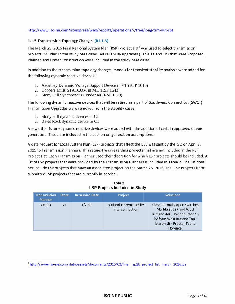
A data request for Local System Plan (LSP) projects that affect the BES was sent by the ISO on April 7, 2015 to Transmission Planners. This request was regarding projects that are not included in the RSP Project List. Each Transmission Planner used their discretion for which LSP projects should be included. A list of LSP projects that were provided by the Transmission Planners is included in Table 2. The list does not include LSP projects that have an associated project on the March 25, 2016 Final RSP Project List or submitted LSP projects that are currently in-service.

Table 2 LSP Projects Included in Study

Transmission Planner

State In-service Date Project Solutions

VELCO VT 1/2019 Rutland-Florence 46 kV Interconnection

Close normally open switches Marble St 237 and West

Rutland 446. Reconductor 46 kV from West Rutland Tap - Marble St - Proctor Tap to

Florence.

4 http://www.iso-ne.com/static-assets/documents/2016/03/final_rsp16_project_list_march_2016.xls

ISO-NE PUBLIC Page 4 of 42

The transmission upgrades associated with the ISO-NE Interconnection Queue projects that had a Proposed Plan Application (PPA) approval as of February 1, 2016 were included in the base cases. These include dynamic devices associated with the following projects:

1. QP 272 – Addition of a dynamic device (Synchronous condenser) interconnecting to the Keene Road 115 kV substation in ME

2. QP 333 – Addition of a dynamic device (SVC) at the Detroit 115 kV substation in ME. Also, addition of a second series capacitor in 388 line and reinstallation of existing series capacitor on 3023 line (originally 388).

3. QP 397 – Addition of a dynamic VAR (DVAR) device at the Bull Hill 115kV substation in ME

The basecases also include a detailed model for the 34.5 kV network in the Central Maine Power (CMP) service area, based on data submitted by CMP.

1.1.6 Forecasted Load [R1.1.4]

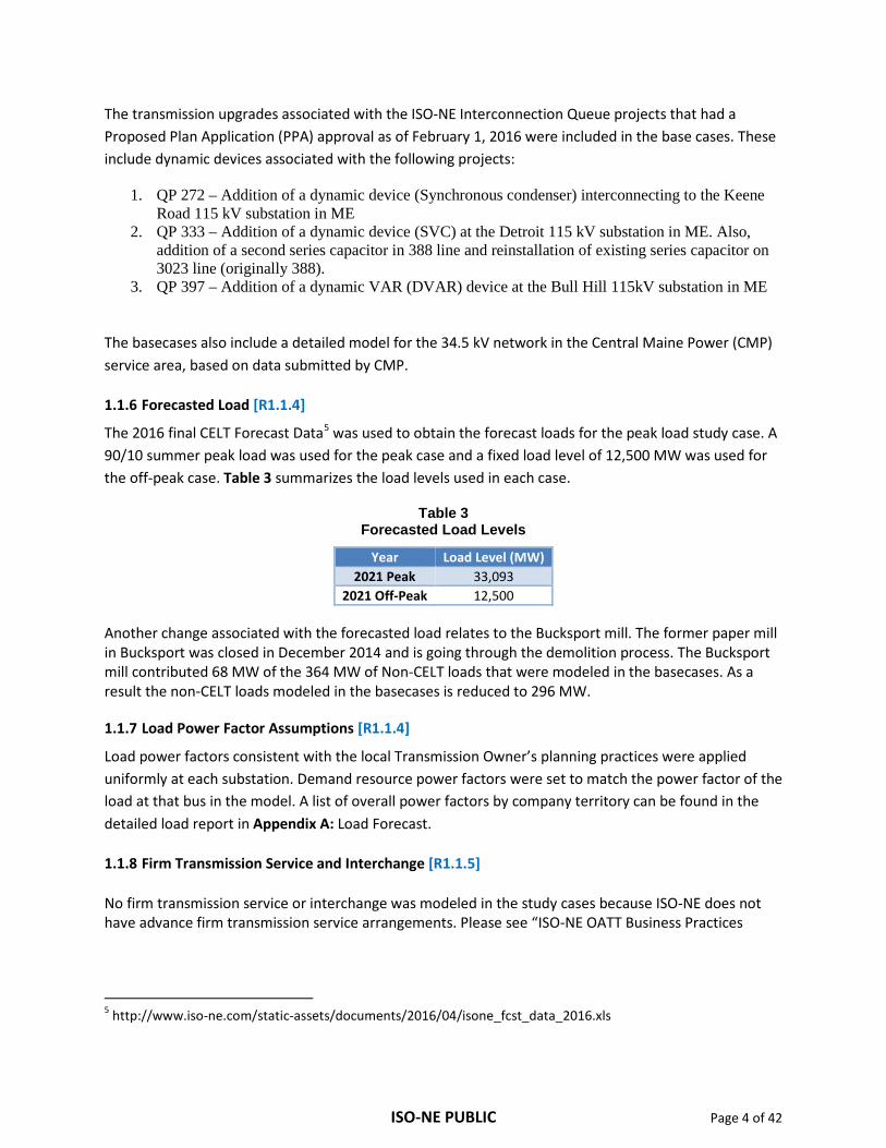
The 2016 final CELT Forecast Data5 was used to obtain the forecast loads for the peak load study case. A 90/10 summer peak load was used for the peak case and a fixed load level of 12,500 MW was used for the off-peak case. Table 3 summarizes the load levels used in each case.

Table 3 Forecasted Load Levels

Year Load Level (MW) 2021 Peak 33,093

2021 Off-Peak 12,500

Another change associated with the forecasted load relates to the Bucksport mill. The former paper mill in Bucksport was closed in December 2014 and is going through the demolition process. The Bucksport mill contributed 68 MW of the 364 MW of Non-CELT loads that were modeled in the basecases. As a result the non-CELT loads modeled in the basecases is reduced to 296 MW.

1.1.7 Load Power Factor Assumptions [R1.1.4]

Load power factors consistent with the local Transmission Owner’s planning practices were applied uniformly at each substation. Demand resource power factors were set to match the power factor of the load at that bus in the model. A list of overall power factors by company territory can be found in the detailed load report in Appendix A: Load Forecast.

1.1.8 Firm Transmission Service and Interchange [R1.1.5]

No firm transmission service or interchange was modeled in the study cases because ISO-NE does not have advance firm transmission service arrangements. Please see “ISO-NE OATT Business Practices

5 http://www.iso-ne.com/static-assets/documents/2016/04/isone_fcst_data_2016.xls

ISO-NE PUBLIC Page 5 of 42

Section 1—OATT Transmission Services Summary6” for details on the transmission services provided by ISO-NE.

1.1.9 Generation Assumptions [R1.1.6]

All existing generators that are included in the ISO-NE MOD system were included in the base cases. All future generators in the ISO Interconnection Queue that had a PPA approval as of February 1, 2016 were included in the base cases

In addition, generators that do not have a PPA approval but have an obligation through the Forward Capacity Market (FCM) and modeling information available were also included in the case. The following generators do not have a PPA approval but are included in the base cases since they cleared in the FCM:

1. QP 489– Combined Cycle in Providence county in RI 2. QP 525 – Combined Cycle Increase in Newport county in RI

One PPA approved project, QP 438-Potter Repowering, was not included since the existing Potter generation was assumed to be online in the basecases. This project cannot be turned online with the existing Potter combined cycle being online. In addition, QP 438 did not clear the FCA-10 auction. For the off-peak stability basecases, the maximum capability of all the units was modeled at its Network Resource Capability (“NRC”) – winter rating. NRC Winter is the maximum amount of energy that a generator has interconnection rights to provide in winter. It is measured as the net output at the Point of Interconnection and represents the generator’s maximum output at or above 0 degrees Fahrenheit. For the peak load stability basecases, the maximum capability of the units was determined by the status of the unit in the FCM. Any unit that cleared in the FCM was modeled at its Summer Qualified Capacity rating and a unit not in the FCM was modeled at its Capacity Network Resource Capability (CNRC) rating (Maximum rating at 90 degrees or greater).

The reactive dispatch for the peak load case of the existing generators is based on the peak load voltage schedules that are published in the latest version (09/11/2015) of the ISO-NE Operating Procedure OP-12 Voltage and Reactive Control Appendix B7. The System Impact Study (SIS) data was used for any future generator.

The reactive dispatch for the off-peak load case of the existing generators is based on the light load voltage schedules that are published in the latest version (09/11/2015) of the ISO-NE Operating Procedure OP-12 Voltage and Reactive Control Appendix B8. The SIS data was used for any future generator.

6http://www.iso-ne.com/static-assets/documents/trans/services/types_apps/rto_bus_prac_sec_1.doc 7 http://www.iso-ne.com/static-assets/documents/rules_proceds/operating/isone/op12/op12b_rto_final.pdf 8 http://www.iso-ne.com/static-assets/documents/rules_proceds/operating/isone/op12/op12b_rto_final.pdf

ISO-NE PUBLIC Page 6 of 42

Photovoltaic (PV) generation is modeled as negative loads in the peak load base case where explicit dynamic models were not available for the PV resources (PV resources under 5 MW nameplate). A description of the PV generation modeling is included in section 1.1.11.

No PV generation is modeled as negative load in the off-peak load case since the load is assumed to be fixed at 12,500 MW of New England load.

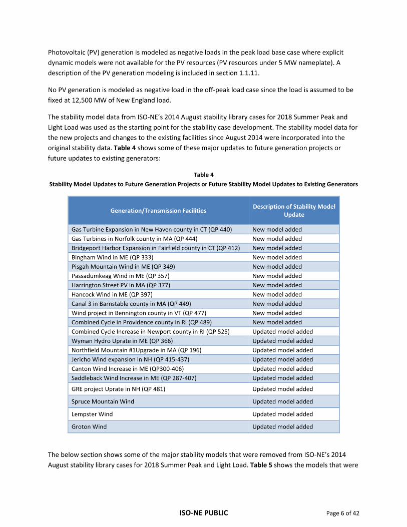
The stability model data from ISO-NE’s 2014 August stability library cases for 2018 Summer Peak and Light Load was used as the starting point for the stability case development. The stability model data for the new projects and changes to the existing facilities since August 2014 were incorporated into the original stability data. Table 4 shows some of these major updates to future generation projects or future updates to existing generators:

Table 4 Stability Model Updates to Future Generation Projects or Future Stability Model Updates to Existing Generators

Generation/Transmission Facilities Description of Stability Model Update

Gas Turbine Expansion in New Haven county in CT (QP 440) New model added Gas Turbines in Norfolk county in MA (QP 444) New model added Bridgeport Harbor Expansion in Fairfield county in CT (QP 412) New model added Bingham Wind in ME (QP 333) New model added Pisgah Mountain Wind in ME (QP 349) New model added Passadumkeag Wind in ME (QP 357) New model added Harrington Street PV in MA (QP 377) New model added Hancock Wind in ME (QP 397) New model added Canal 3 in Barnstable county in MA (QP 449) New model added Wind project in Bennington county in VT (QP 477) New model added Combined Cycle in Providence county in RI (QP 489) New model added Combined Cycle Increase in Newport county in RI (QP 525) Updated model added Wyman Hydro Uprate in ME (QP 366) Updated model added Northfield Mountain #1Upgrade in MA (QP 196) Updated model added Jericho Wind expansion in NH (QP 415-437) Updated model added Canton Wind Increase in ME (QP300-406) Updated model added Saddleback Wind Increase in ME (QP 287-407) Updated model added

GRE project Uprate in NH (QP 481) Updated model added

Spruce Mountain Wind Updated model added

Lempster Wind Updated model added

Groton Wind Updated model added

The below section shows some of the major stability models that were removed from ISO-NE’s 2014 August stability library cases for 2018 Summer Peak and Light Load. Table 5 shows the models that were

ISO-NE PUBLIC Page 7 of 42

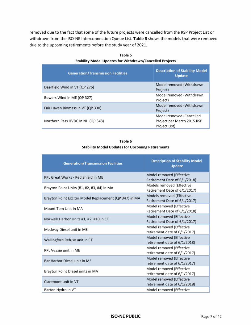
removed due to the fact that some of the future projects were cancelled from the RSP Project List or withdrawn from the ISO-NE Interconnection Queue List. Table 6 shows the models that were removed due to the upcoming retirements before the study year of 2021.

Table 5 Stability Model Updates for Withdrawn/Cancelled Projects

Generation/Transmission Facilities Description of Stability Model Update

Deerfield Wind in VT (QP 276) Model removed (Withdrawn Project)

Bowers Wind in ME (QP 327) Model removed (Withdrawn Project)

Fair Haven Biomass in VT (QP 330) Model removed (Withdrawn Project)

Northern Pass HVDC in NH (QP 348) Model removed (Cancelled Project per March 2015 RSP Project List)

Table 6 Stability Model Updates for Upcoming Retirements

Generation/Transmission Facilities Description of Stability Model Update

PPL Great Works - Red Shield in ME Model removed (Effective Retirement Date of 6/1/2018)

Brayton Point Units (#1, #2, #3, #4) in MA Models removed (Effective Retirement Date of 6/1/2017)

Brayton Point Exciter Model Replacement (QP 347) in MA Models removed (Effective Retirement Date of 6/1/2017)

Mount Tom Unit in MA Model removed (Effective Retirement Date of 6/1/2018)

Norwalk Harbor Units #1, #2, #10 in CT Model removed (Effective Retirement Date of 6/1/2017)

Medway Diesel unit in ME Model removed (Effective retirement date of 6/1/2017)

Wallingford Refuse unit in CT Model removed (Effective retirement date of 6/1/2018)

PPL Veazie unit in ME Model removed (Effective retirement date of 6/1/2017)

Bar Harbor Diesel unit in ME Model removed (Effective retirement date of 6/1/2017)

Brayton Point Diesel units in MA Model removed (Effective retirement date of 6/1/2017)

Claremont unit in VT Model removed (Effective retirement date of 6/1/2018)

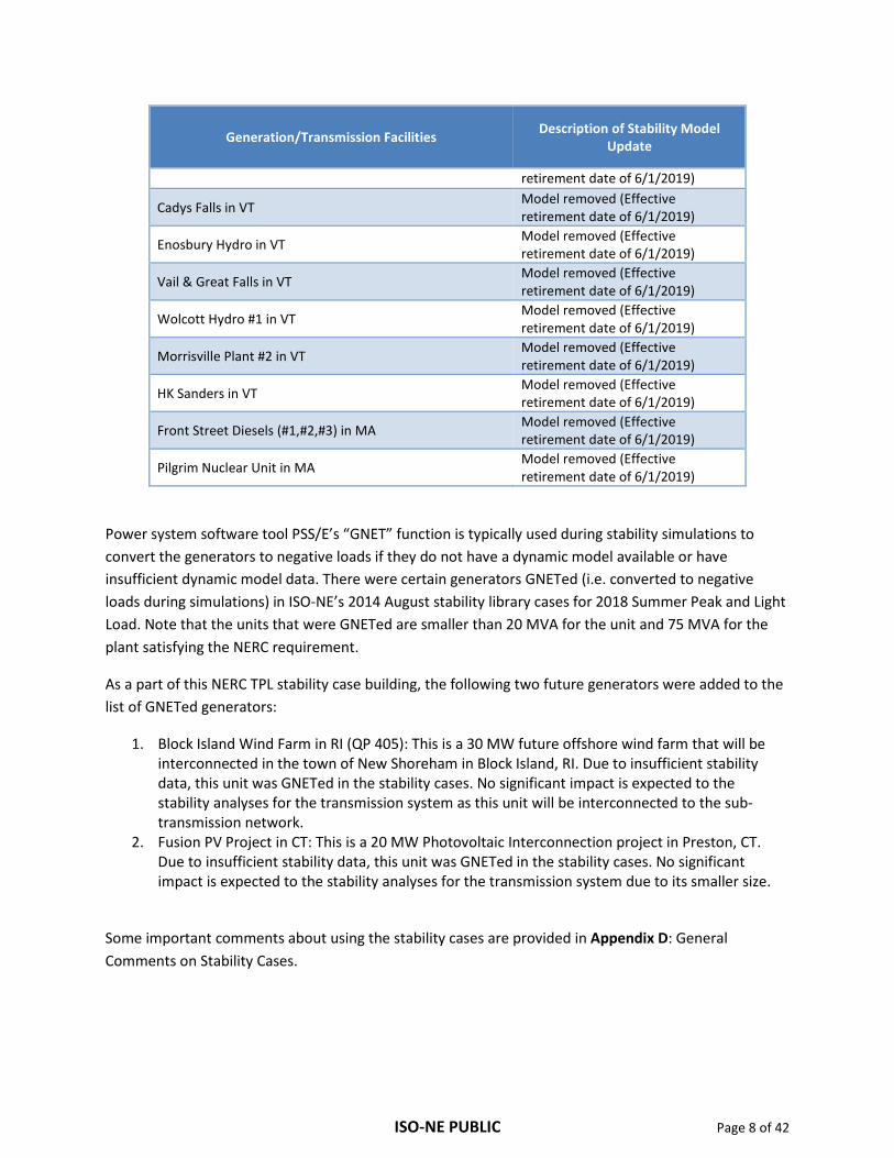
Barton Hydro in VT Model removed (Effective

ISO-NE PUBLIC Page 8 of 42

Generation/Transmission Facilities Description of Stability Model Update

retirement date of 6/1/2019)

Cadys Falls in VT Model removed (Effective retirement date of 6/1/2019)

Enosbury Hydro in VT Model removed (Effective retirement date of 6/1/2019)

Vail & Great Falls in VT Model removed (Effective retirement date of 6/1/2019)

Wolcott Hydro #1 in VT Model removed (Effective retirement date of 6/1/2019)

Morrisville Plant #2 in VT Model removed (Effective retirement date of 6/1/2019)

HK Sanders in VT Model removed (Effective retirement date of 6/1/2019)

Front Street Diesels (#1,#2,#3) in MA Model removed (Effective retirement date of 6/1/2019)

Pilgrim Nuclear Unit in MA Model removed (Effective retirement date of 6/1/2019)

Power system software tool PSS/E’s “GNET” function is typically used during stability simulations to convert the generators to negative loads if they do not have a dynamic model available or have insufficient dynamic model data. There were certain generators GNETed (i.e. converted to negative loads during simulations) in ISO-NE’s 2014 August stability library cases for 2018 Summer Peak and Light Load. Note that the units that were GNETed are smaller than 20 MVA for the unit and 75 MVA for the plant satisfying the NERC requirement.

As a part of this NERC TPL stability case building, the following two future generators were added to the list of GNETed generators:

1. Block Island Wind Farm in RI (QP 405): This is a 30 MW future offshore wind farm that will be interconnected in the town of New Shoreham in Block Island, RI. Due to insufficient stability data, this unit was GNETed in the stability cases. No significant impact is expected to the stability analyses for the transmission system as this unit will be interconnected to the sub-transmission network.

2. Fusion PV Project in CT: This is a 20 MW Photovoltaic Interconnection project in Preston, CT. Due to insufficient stability data, this unit was GNETed in the stability cases. No significant impact is expected to the stability analyses for the transmission system due to its smaller size.

Some important comments about using the stability cases are provided in Appendix D: General Comments on Stability Cases.

ISO-NE PUBLIC Page 9 of 42

1.1.10 Demand Resource Assumptions [R1.1.6]

Demand resources (DR) were only modeled for the peak load case since the off-peak load case at 12,500 MW includes the impact of all DR. Demand resources that are modeled in the study can be divided into three categories:

1. Passive DR that cleared in the Forward Capacity Market through FCA 10 (June 1, 2019 – May 31, 2020)

2. Active DR that cleared in the Forward Capacity Market through FCA 10 (June 1, 2019 – May 31, 2020)

3. 2016 Final CELT Energy Efficiency (EE) forecast for the period beyond May 31, 2020.

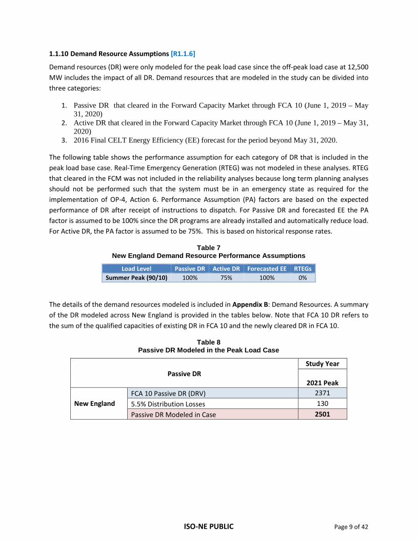
The following table shows the performance assumption for each category of DR that is included in the peak load base case. Real-Time Emergency Generation (RTEG) was not modeled in these analyses. RTEG that cleared in the FCM was not included in the reliability analyses because long term planning analyses should not be performed such that the system must be in an emergency state as required for the implementation of OP-4, Action 6. Performance Assumption (PA) factors are based on the expected performance of DR after receipt of instructions to dispatch. For Passive DR and forecasted EE the PA factor is assumed to be 100% since the DR programs are already installed and automatically reduce load. For Active DR, the PA factor is assumed to be 75%. This is based on historical response rates.

Table 7 New England Demand Resource Performance Assumptions

Load Level Passive DR Active DR Forecasted EE RTEGs Summer Peak (90/10) 100% 75% 100% 0%

The details of the demand resources modeled is included in Appendix B: Demand Resources. A summary of the DR modeled across New England is provided in the tables below. Note that FCA 10 DR refers to the sum of the qualified capacities of existing DR in FCA 10 and the newly cleared DR in FCA 10.

Table 8 Passive DR Modeled in the Peak Load Case

Passive DR

Study Year

2021 Peak

New England FCA 10 Passive DR (DRV) 2371 5.5% Distribution Losses 130 Passive DR Modeled in Case 2501

ISO-NE PUBLIC Page 10 of 42

Table 9 EE Forecast Modeled in the Peak Load Case

EE Forecast

Study Year

2021 Peak

New England EE Forecast for years 2020 - 2021 (DRV) 450 5.5% Distribution Losses 25 EE Forecast Modeled in Case 475

Table 10 Active DR Modeled in the Peak Load Case

Active DR

Study Year

2021 Peak

New England

FCA10 Active DR (DRV) in New England 406 5.5% Distribution Losses + 22 Unavailable Active DR (25%) -107 Active DR Modeled in Case 321

1.1.11 Photovoltaic (PV) Generation Modeling and Assumptions [R1.1.6]

In addition to the resources that cleared the FCM, the PV generation forecast was used to model PV generation in the summer peak load case. Similar to DR, the PV generation forecast was only modeled for the summer peak load case. The 2016 Final CELT PV generation forecast includes the PV generation that has been installed as of the end of 2015 and provides a forecast by state of the total PV (by AC Nameplate9) that is expected to be in-service by the end of each forecast year for the next 10 years. As an example, the 2016 final PV forecast provides the PV that is in-service as of the end of 2015 as well as provides an annual forecast for the PV that will be in-service for end of 2016, end of 2017 and so on until the end of 2025.

For a given peak load study year the PV is modeled based on the PV that is expected to be in-service by the end of the year prior to the study year, plus the PV that is expected to be in-service by May 31st of the study year. As an example, the 2021 summer peak load case will include all the PV that is expected to be in-service by 2020 plus the portion of the PV that is expected to be in-service by May 31, 2021. To determine the portion of the annual PV forecast that will be in-service by the end of May 31, 2021, the following table from the 2015 CELT Report is utilized. Based on the table, 27% (cumulative growth up to May) of the forecasted PV for the year 2021 will be assumed to be in-service for the 2021 summer peak basecase.

9 AC nameplate is the nameplate output of a PV facility as measured on the AC side of the inverter.

ISO-NE PUBLIC Page 11 of 42

Table 11 Monthly PV Growth Table (as a % of Annual Growth)

Month Incremental Cumulative 1 5% 5% 2 4% 9% 3 5% 14% 4 6% 20% 5 6% 27% 6 9% 36% 7 10% 45% 8 10% 55% 9 7% 62%

10 8% 70% 11 7% 77% 12 23% 100%

Based on a review of historic PV outputs, ISO-NE Transmission Planning has determined a 26% availability factor to be applied to model PV generation in transmission planning studies. The details of the PV generation modeling are included in Appendix C: PV generation modeling. The individual PV plants that are greater than 5 MW are modeled as generators in the base case. The PV less than 5 MW are modeled as negative loads. Table 12 summarizes the PV generation modeled as negative loads for the peak load case.

Table 12

PV generation Modeled in the Peak Load Case

PV generation Modeled as Negative Loads

Study Year

2021 Peak

New England

A - PV generation (nameplate) in New England 2572 B - 5.5% Reduction in Distribution Losses 141 C - Unavailable PV generation (A+B)*(1-26%) 2008 PV generation Modeled in Case as Negative Loads (A+B)-C 70510

1.1.12 Explanation of Future Changes Not Included

Two transmission projects listed on the March 25, 2016 RSP Project List were not included in the study cases:

• RSP 1269: The project to add a new 345 kV breaker and two 25 MVAR capacitor banks at the Amherst substation in New Hampshire was not included because the Transmission Owner has raised concerns regarding the feasibility of implementing the Amherst 345 kV capacitor banks proposed in the previous New Hampshire/Vermont Solutions Study.

10 This value includes explicitly modeled PV generators.

ISO-NE PUBLIC Page 12 of 42

• RSP 1280: The project to add a new 115 kV line section 244 and upgrading line section 80 between Coopers Mill and Highland Substations was not included because the Transmission Owner indicated that the project may not move forward.

1.1.13 Load Levels Studied [R2.1.1, R2.1.2 and R2.2]

This section summarizes the net load level studied for each base case. The tables below exclude the Station Service loads which vary based on dispatch assumptions.

Table 13: Net Load Modeled for 2021 peak load (Excludes Transmission Losses)

Category Load (MW) 90/10 CELT Forecast 32,327 Non-CELT Manufacturing load in New England 296 Available FCA-10 Passive DR (modeled as negative load) -2,501 Available FCA-10 Active DR (modeled as negative load) -321 Final 2016 CELT EE Forecast for year 2021 (modeled as negative load) -475 Final 2016 CELT PV Forecast for year 2021 (modeled as negative load) -705 Net load modeled in New England (Excludes Station Service Load) 28,621

Table 14: Net Load Modeled for 2021 off-peak load (Excludes Transmission Losses)

Category Load (MW) Fixed CELT Load based on historical data 11,922 Non-CELT Manufacturing load in New England 296 Available FCA-10 Passive DR (modeled as negative load) 0 Available FCA-10 Active DR (modeled as negative load) 0 Final 2016 CELT EE Forecast for year 2021 (modeled as negative load) 0 Final 2016 CELT PV Forecast for year 2021 (modeled as negative load) 0 Net load modeled in New England (Excludes Station Service Load) 12,218

1.1.14 Dynamic Load Model [R2.4.1]

A dynamic load model was added to the peak load stability case to model the dynamic behavior of Loads that could impact the study area, including the consideration of the behavior of induction motor Loads.

A key source of data for the dynamic load model for New England is a report that was prepared by DNV-GL for Lawrence Berkeley National Laboratory. The report was titled “End Use Data Development for Power System Load Model in New England – Methodology and Results11”. As a part of this report the New England load was characterized by:

1. Summer Peak and Spring Light Load hour 2. Seven geographic areas - Maine, New Hampshire, Vermont, Connecticut, Rhode Island, Eastern

Massachusetts and Western Massachusetts 3. Customer sector – Residential, Commercial and Industrial

11 http://eetd.lbl.gov/sites/all/files/data-development-for-ne-end-use-load-modeling.pdf

ISO-NE PUBLIC Page 13 of 42

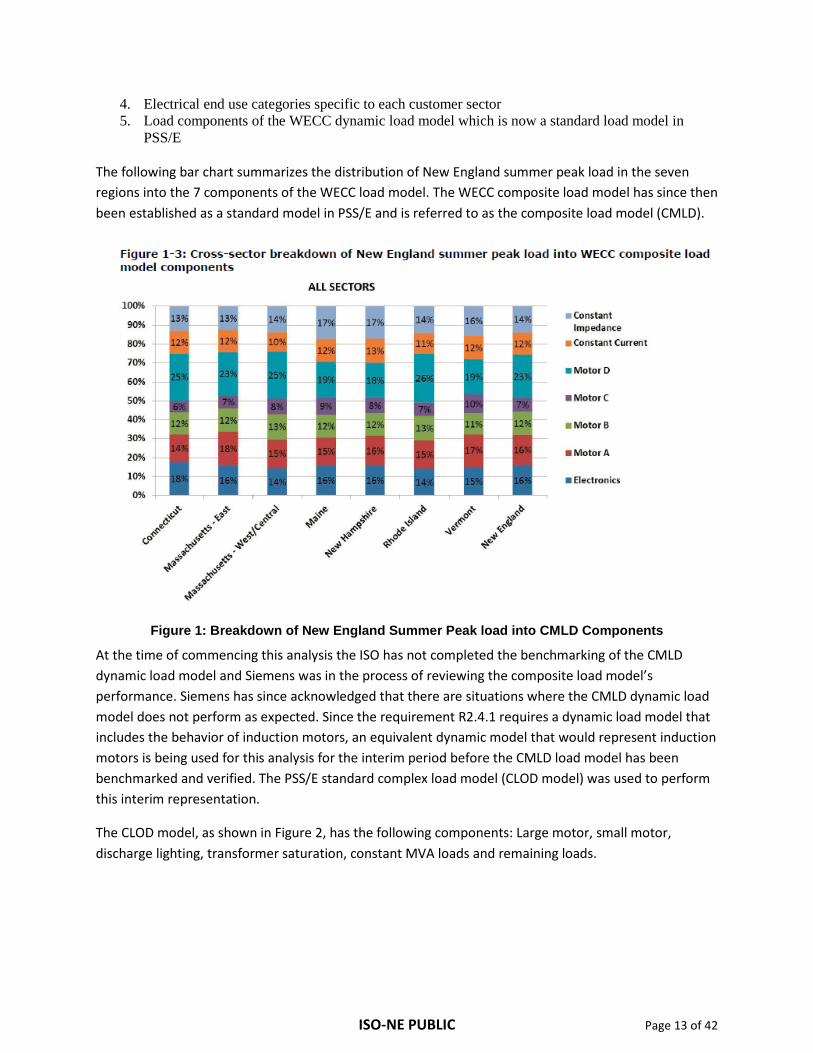
4. Electrical end use categories specific to each customer sector 5. Load components of the WECC dynamic load model which is now a standard load model in

PSS/E

The following bar chart summarizes the distribution of New England summer peak load in the seven regions into the 7 components of the WECC load model. The WECC composite load model has since then been established as a standard model in PSS/E and is referred to as the composite load model (CMLD).

Figure 1: Breakdown of New England Summer Peak load into CMLD Components

At the time of commencing this analysis the ISO has not completed the benchmarking of the CMLD dynamic load model and Siemens was in the process of reviewing the composite load model’s performance. Siemens has since acknowledged that there are situations where the CMLD dynamic load model does not perform as expected. Since the requirement R2.4.1 requires a dynamic load model that includes the behavior of induction motors, an equivalent dynamic model that would represent induction motors is being used for this analysis for the interim period before the CMLD load model has been benchmarked and verified. The PSS/E standard complex load model (CLOD model) was used to perform this interim representation.

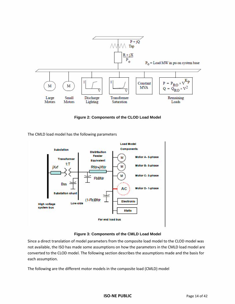
The CLOD model, as shown in Figure 2, has the following components: Large motor, small motor, discharge lighting, transformer saturation, constant MVA loads and remaining loads.

ISO-NE PUBLIC Page 14 of 42

Figure 2: Components of the CLOD Load Model

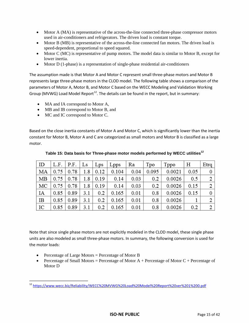
The CMLD load model has the following parameters

Figure 3: Components of the CMLD Load Model

Since a direct translation of model parameters from the composite load model to the CLOD model was not available, the ISO has made some assumptions on how the parameters in the CMLD load model are converted to the CLOD model. The following section describes the assumptions made and the basis for each assumption.

The following are the different motor models in the composite load (CMLD) model

ISO-NE PUBLIC Page 15 of 42

• Motor A (MA) is representative of the across-the-line connected three-phase compressor motors used in air-conditioners and refrigerators. The driven load is constant torque.

• Motor B (MB) is representative of the across-the-line connected fan motors. The driven load is speed-dependent, proportional to speed squared.

• Motor C (MC) is representative of pump motors. The model data is similar to Motor B, except for lower inertia.

• Motor D (1-phase) is a representation of single-phase residential air-conditioners

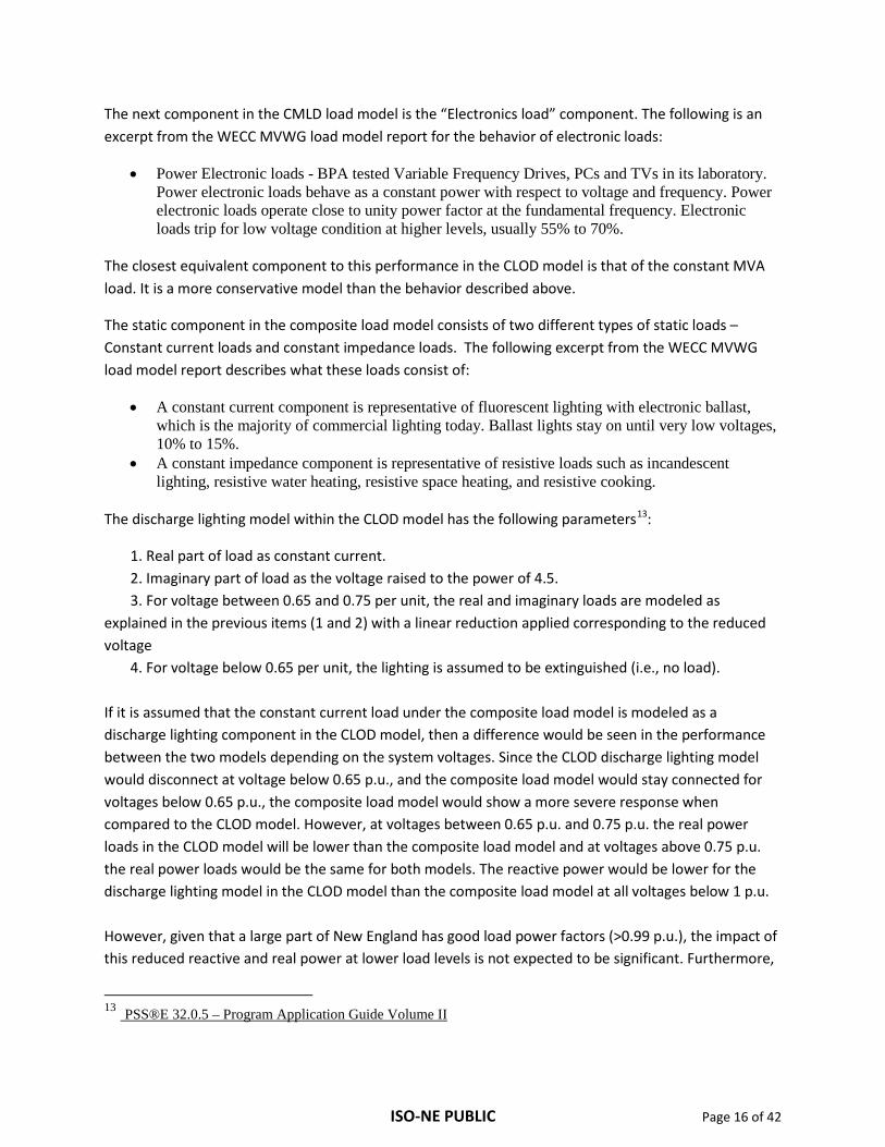
The assumption made is that Motor A and Motor C represent small three-phase motors and Motor B represents large three-phase motors in the CLOD model. The following table shows a comparison of the parameters of Motor A, Motor B, and Motor C based on the WECC Modeling and Validation Working Group (MVWG) Load Model Report12. The details can be found in the report, but in summary:

• MA and IA correspond to Motor A, • MB and IB correspond to Motor B, and • MC and IC correspond to Motor C.

Based on the close inertia constants of Motor A and Motor C, which is significantly lower than the inertia constant for Motor B, Motor A and C are categorized as small motors and Motor B is classified as a large motor.

Table 15: Data basis for Three-phase motor models performed by WECC utilities12

Note that since single phase motors are not explicitly modeled in the CLOD model, these single phase units are also modeled as small three-phase motors. In summary, the following conversion is used for the motor loads:

• Percentage of Large Motors = Percentage of Motor B • Percentage of Small Motors = Percentage of Motor A + Percentage of Motor C + Percentage of

Motor D

12 https://www.wecc.biz/Reliability/WECC%20MVWG%20Load%20Model%20Report%20ver%201%200.pdf

ISO-NE PUBLIC Page 16 of 42

The next component in the CMLD load model is the “Electronics load” component. The following is an excerpt from the WECC MVWG load model report for the behavior of electronic loads:

• Power Electronic loads - BPA tested Variable Frequency Drives, PCs and TVs in its laboratory. Power electronic loads behave as a constant power with respect to voltage and frequency. Power electronic loads operate close to unity power factor at the fundamental frequency. Electronic loads trip for low voltage condition at higher levels, usually 55% to 70%.

The closest equivalent component to this performance in the CLOD model is that of the constant MVA load. It is a more conservative model than the behavior described above.

The static component in the composite load model consists of two different types of static loads – Constant current loads and constant impedance loads. The following excerpt from the WECC MVWG load model report describes what these loads consist of:

• A constant current component is representative of fluorescent lighting with electronic ballast, which is the majority of commercial lighting today. Ballast lights stay on until very low voltages, 10% to 15%.

• A constant impedance component is representative of resistive loads such as incandescent lighting, resistive water heating, resistive space heating, and resistive cooking.

The discharge lighting model within the CLOD model has the following parameters13:

1. Real part of load as constant current. 2. Imaginary part of load as the voltage raised to the power of 4.5. 3. For voltage between 0.65 and 0.75 per unit, the real and imaginary loads are modeled as

explained in the previous items (1 and 2) with a linear reduction applied corresponding to the reduced voltage

4. For voltage below 0.65 per unit, the lighting is assumed to be extinguished (i.e., no load). If it is assumed that the constant current load under the composite load model is modeled as a discharge lighting component in the CLOD model, then a difference would be seen in the performance between the two models depending on the system voltages. Since the CLOD discharge lighting model would disconnect at voltage below 0.65 p.u., and the composite load model would stay connected for voltages below 0.65 p.u., the composite load model would show a more severe response when compared to the CLOD model. However, at voltages between 0.65 p.u. and 0.75 p.u. the real power loads in the CLOD model will be lower than the composite load model and at voltages above 0.75 p.u. the real power loads would be the same for both models. The reactive power would be lower for the discharge lighting model in the CLOD model than the composite load model at all voltages below 1 p.u. However, given that a large part of New England has good load power factors (>0.99 p.u.), the impact of this reduced reactive and real power at lower load levels is not expected to be significant. Furthermore,

13 PSS®E 32.0.5 – Program Application Guide Volume II

ISO-NE PUBLIC Page 17 of 42

the reduction of electronic loads at low voltages and the potential tripping of motor loads with low voltages are not modeled with the CLOD model and the additional conservativism in modeling motor loads and electronic loads is expected to offset the reduced constant current loads modeled in the CLOD model. In summary, the constant current load component in the composite load model will be modeled as a discharge lighting load in the CLOD equivalent model. The only remaining component is the constant impedance component in the composite load model. This component is modeled as a voltage sensitive load in the CLOD model where the load is set to vary by square of the voltage. There is no component in the composite load model to represent transformer saturation. Hence the transformer saturation component of the CLOD dynamic load model is set to 0. In summary, the following methodology was used to convert the composite load model parameters to the CLOD parameters:

• Percentage of Large Motors = Percentage of Motor B • Percentage of Small Motors = Percentage of Motor A + Percentage of Motor C + Percentage of

Motor D • Constant MVA = Electronics • Discharge Lighting = Constant Current Load • Transformer Saturation = 0 • Remaining Loads = Constant Impedance Loads with a Kp of remaining loads = 2 (for constant

impedance loads)

Two other parameters that are a part of the CLOD model but do not deal with the load components is the R+jX parameter that could be used to account for feeder impedances. Typically modeling feeder impedances would:

• Modify the effective power factor of the load • Reduce the terminal voltage of the load by accounting for voltage drop along the feeder • Account for losses along the feeder and reduce the net load that the dynamic load model is

applied to (c)

In the CLOD model, the motor component, constant MVA component, and discharge lighting component are all initialized to a predetermined power factor. The only variation in power factor is observed on the remaining load which is modeled as a constant impedance load based on the assumptions discussed in this document.

Based on PSS/E documentation, the CLOD model is always initialized to a 0.98 p.u. voltage at the terminal. To attain this terminal voltage, the “tap” is adjusted automatically by the software. As a result, the modeling of the feeder impedances will not affect the terminal voltage of the load at initialization. During disturbances as the load varies some impact will be observed of having the feeder impedances modeled, but since the additional reactive loss caused by the feeder at initialization is compensated by an additional reactive compensation at the load terminal will diminish this impact to some extent.

ISO-NE PUBLIC Page 18 of 42

In all, the impact of the reduced load modeled (due to real power loss on the feeder) and the addition of the capacitive compensation of the load end to account for reactive losses at initialization is expected to account for any decrease in voltage caused by the feeder impedances. Thus the assumption of ignoring feeder impedances and having the distribution system losses inherently accounted for in the load is considered to be an acceptable modeling state. In summary, R and X will be set to 0.

Once we have established the methodology to convert the composite load model parameters to the CLOD complex load model parameters the next step is to use the composite load components from the New England end use load model to determine the actual components.

New England loads consist of the following components:

1. CELT load for the six New England states 2. Passive DR, Active DR and EE forecast for the six New England states modeled as negative

loads 3. PV forecast modeled as negative loads 4. Manufacturing loads in ME (Non-CELT) 5. Station Service loads

The first step in the load modeling was to eliminate all the negative loads associated with demand resources by reducing the load at the different buses by an equivalent amount. The next step was to reclassify all the New England CELT loads into the 7 regions defined in the New England end-use load model report. The CELT loads were reclassified into the following owners:

1. Owner 60 – ME CELT loads net of DR 2. Owner 61 – NH CELT loads net of DR 3. Owner 62 – VT CELT loads net of DR 4. Owner 63 – Eastern MA CELT loads net of DR 5. Owner 64 – Western MA CELT loads net of DR 6. Owner 65 – Rhode Island CELT loads net of DR 7. Owner 66 – Connecticut CELT loads net of DR

The remaining non-negative loads are either Manufacturing loads in ME or station service loads across New England. To determine the components of the composite load model that correspond to these loads, the equivalent parameters of the industrial load in New England was used. The following table summarizes the estimated Industrial Peak hour load component distribution.

ISO-NE PUBLIC Page 19 of 42

Figure 4: Breakdown of New England Summer Peak load into CMLD Components

The components based on Maine industrial loads are used to model the Maine manufacturing loads. The components based on New England industrial loads are used to model the station service loads for all New England generators. These loads were classified into the following owners:

1. Owner 67 – ME Manufacturing Loads 2. Owner 68 – Common owner for all New England Station Service Loads

The only remaining loads in the case are negative loads corresponding to PV loads and one negative load associated with equivalent generation in ME. A typical inverter based device, when subject to declining terminal voltages, would be constant power until the current limit is reached and then would operate in constant current mode. If the PV device were operating at 100% output there would be very little available capacity on the converter so as voltage would decrease on the system the current limit on the inverter would soon be reached. But since a 26% availability is assumed for the PV inverter, the inverter can maintain a constant power output for larger deviations in voltage from nominal. Hence the inverter can be assumed to be in constant power mode for the equivalent model in ZIP load model parameters. Typically, distributed PV inverters would operate at unity power factor and not produce any reactive power. To account for avoided reactive losses on the distribution system we attribute some reactive output to these PV inverters when modeled as negative loads at the low side of the distribution substation. Since the reactive component of the negative loads that represent PV is not based on inverter output, this component will be modeled as constant impedance.

Some limited number of loads in the basecase with zero real power output was given owner 69 and no dynamic loads were applied to these loads. These reactive loads were modeled as constant impedance loads.

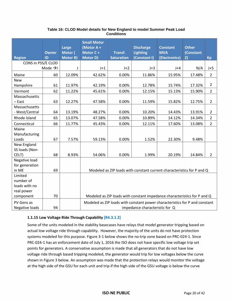
The final table below shows the different components in the CLOD model for the different areas and loads in New England:

ISO-NE PUBLIC Page 20 of 42

Table 16: CLOD Model details for New England to model Summer Peak Load Conditions

Region Owner ID

Large Motor ( Motor B)

Small Motor (Motor A + Motor C + Motor D)

Transf. Saturation

Discharge Lighting (Constant I)

Constant MVA (Electronics)

Other (Constant Z) Kp

CONS in PSS/E CLOD Mode l J J+1 J+2 J+3 J+4 N/A J+5

Maine 60 12.09% 42.62% 0.00% 11.86% 15.95% 17.48% 2 New Hampshire 61 11.97% 42.19% 0.00% 12.78% 15.74% 17.32% 2

Vermont 62 11.22% 45.61% 0.00% 12.15% 15.13% 15.90% 2 Massachusetts – East 63 12.27% 47.58% 0.00% 11.59% 15.82% 12.75% 2 Massachusetts - West/Central 64 13.19% 48.27% 0.00% 10.20% 14.43% 13.91% 2 Rhode Island 65 13.07% 47.58% 0.00% 10.89% 14.12% 14.34% 2 Connecticut 66 11.77% 45.43% 0.00% 12.11% 17.60% 13.08% 2 Maine Manufacturing Loads 67 7.57% 59.13% 0.00% 1.52% 22.30% 9.48% New England SS loads (Non-CELT) 68 8.93% 54.06% 0.00% 1.99% 20.19% 14.84% 2 Negative load for generation in ME 69

Modeled as ZIP loads with constant current characteristics for P and Q Limited number of loads with no real power component 70

Modeled as ZIP loads with constant impedance characteristics for P and Q PV Gens as Negative loads 94

Modeled as ZIP loads with constant power characteristics for P and constant impedance characteristic for Q

1.1.15 Low Voltage Ride Through Capability [R4.3.1.2]

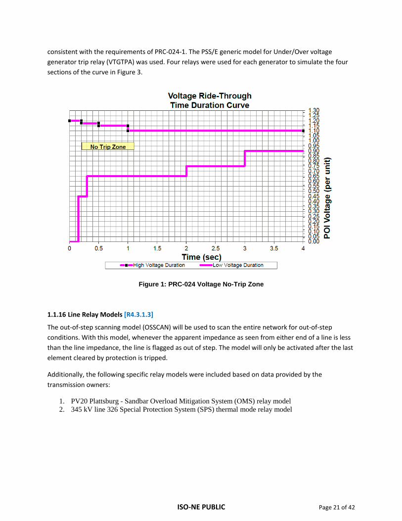
Some of the units modeled in the stability basecases have relays that model generator tripping based on actual low voltage ride through capability. However, the majority of the units do not have protection systems modeled for this purpose. Figure 3-1 below shows the no-trip zone based on PRC-024-1. Since PRC-024-1 has an enforcement date of July 1, 2016 the ISO does not have specific low voltage trip set points for generators. A conservative assumption is made that all generators that do not have low voltage ride through based tripping modeled, the generator would trip for low voltages below the curve shown in Figure 3 below. An assumption was made that the protection relays would monitor the voltage at the high side of the GSU for each unit and trip if the high side of the GSU voltage is below the curve

ISO-NE PUBLIC Page 21 of 42

consistent with the requirements of PRC-024-1. The PSS/E generic model for Under/Over voltage generator trip relay (VTGTPA) was used. Four relays were used for each generator to simulate the four sections of the curve in Figure 3.

Figure 1: PRC-024 Voltage No-Trip Zone

1.1.16 Line Relay Models [R4.3.1.3]

The out-of-step scanning model (OSSCAN) will be used to scan the entire network for out-of-step conditions. With this model, whenever the apparent impedance as seen from either end of a line is less than the line impedance, the line is flagged as out of step. The model will only be activated after the last element cleared by protection is tripped.

Additionally, the following specific relay models were included based on data provided by the transmission owners:

1. PV20 Plattsburg - Sandbar Overload Mitigation System (OMS) relay model 2. 345 kV line 326 Special Protection System (SPS) thermal mode relay model

ISO-NE PUBLIC Page 22 of 42

1.1.17 Dynamic Stability Simulation Voltage Sag Model [R5]

A PSS/E user-written model is utilized to monitor the transient voltage response of the system consistent with ISO-NE voltage sag guideline14. This model monitors the voltages of all 115 kV and above buses during the stability simulations, and flags as violations if the post-fault bus voltage goes below 0.70 pu or if the post-fault bus voltage remains below 0.80 pu for a period greater than 250 milliseconds.

Furthermore, this model has an additional functionality to monitor the post-fault bus voltage recovery. As ISO-NE is in the process of determining a criterion for post-fault voltage recovery, the following assumptions may change once a final criterion has been established. For this study, an assumption has been made such that the model will flag all the 115 kV and above buses if the post-fault voltage remains below 0.80 pu for at least 10 seconds.

The details of the user-written model are included in Appendix E. Note that the voltage set points and times used in Appendix E are just examples and may not match with the actual values used in the stability base cases as discussed above.

1.1.18 Maine Mill Load Modeling

The major industrial loads in Maine are modeled according to the actual contract values in the peak and light load stability base cases. In order to match these net contract values, the mill generators were adjusted in each base case such that the net inflow into each Mill load pocket would be close to the net mill load contract values. Note that in some scenarios these contract values were not achieved due to the amount of load and generator modeled in that pocket. The target net mill load levels modeled in the base cases are shown in the below table.

Mill Load Pocket Contract MW New Page 100

Sappi Somerset 65 Verso IP Jay 72

Madison Electric 87 Sappi Westbrook 38

14 http://www.iso-ne.com/static-assets/documents/committees/comm_wkgrps/prtcpnts_comm/pac/plan_guides/plan_tech_guide/technical_planning_guide_appendix_e_voltage_sag_guideline.pdf

ISO-NE PUBLIC Page 23 of 42

Section 2 Appendix A: Load Forecast 2021 Summer Peak Load

ISO-NE PUBLIC Page 24 of 42

2021 Off-Peak Load

ISO-NE PUBLIC Page 25 of 42

Section 3 Appendix B: Demand Resources The following three tables indicate how each DR type is modeled in the peak load base case. The DR modeled in the peak load case by load zone is provided. The DR values that are released as a part of the FCA results and the Final 2016 CELT EE forecast have transmission and distribution losses (8%) included. For modeling in the study base case, only the distribution losses (assumed to be 5.5%) will be added to the DR since the transmission losses (2.5%) will be computed by the simulation software.

Table 15: Passive DR Modeled in the Peak Load Case

Passive DR Study Year

Load Zone 2021 Peak

Connecticut FCA 10 Passive DR (DRV) 494 5.5% Distribution Losses + 27 Passive DR Modeled in Case 521

Maine FCA 10 Passive DR (DRV) 169 5.5% Distribution Losses + 10 Passive DR Modeled in Case 179

New Hampshire

FCA 10 Passive DR (DRV) 101 5.5% Distribution Losses + 6 Passive DR Modeled in Case 107

Vermont FCA 10 Passive DR (DRV) 112 5.5% Distribution Losses + 6 Passive DR Modeled in Case 118

Rhode Island FCA 10 Passive DR (DRV) 210 5.5% Distribution Losses + 11 Passive DR Modeled in Case 221

NEMA/BOSTON FCA 10 Passive DR (DRV) 589 5.5% Distribution Losses + 32 Passive DR Modeled in Case 621

SEMA FCA 10 Passive DR (DRV) 314 5.5% Distribution Losses + 17 Passive DR Modeled in Case 331

WCMA FCA 10 Passive DR (DRV) 383 5.5% Distribution Losses + 21 Passive DR Modeled in Case 404

New England FCA 10 Passive DR (DRV) 2371 5.5% Distribution Losses 130 Passive DR Modeled in Case 2501

ISO-NE PUBLIC Page 26 of 42

Table 16: EE Forecast Modeled in the Peak Load Case

EE Forecast Study Year

Load Zone 2021 Peak

Connecticut EE Forecast for years 2020-2021 86 5.5% Distribution Losses + 5 EE Forecast Modeled in Case 91

Maine EE Forecast for years 2020-2021 26 5.5% Distribution Losses + 1 EE Forecast Modeled in Case 27

New Hampshire

EE Forecast for years 2020-2021 15 5.5% Distribution Losses + 1 EE Forecast Modeled in Case 16

Vermont EE Forecast for years 2020-2021 25 5.5% Distribution Losses + 1 EE Forecast Modeled in Case 26

Rhode Island EE Forecast for years 2020-2021 39 5.5% Distribution Losses + 2 EE Forecast Modeled in Case 41

NEMA/BOSTON EE Forecast for years 2020-2021 119 5.5% Distribution Losses + 7 EE Forecast Modeled in Case 126

SEMA EE Forecast for years 2020-2021 63 5.5% Distribution Losses + 3 EE Forecast Modeled in Case 66

WCMA EE Forecast for years 2020-2021 78 5.5% Distribution Losses + 4 EE Forecast Modeled in Case 82

New England EE Forecast for years 2020-2021 450 5.5% Distribution Losses 25 EE Forecast Modeled in Case 475

ISO-NE PUBLIC Page 27 of 42

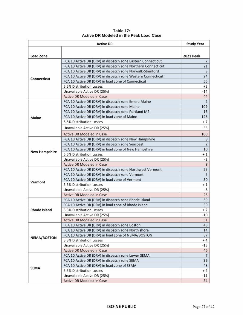
Table 17: Active DR Modeled in the Peak Load Case

Active DR Study Year

Load Zone 2021 Peak

Connecticut

FCA 10 Active DR (DRV) in dispatch zone Eastern Connecticut 7 FCA 10 Active DR (DRV) in dispatch zone Northern Connecticut 21 FCA 10 Active DR (DRV) in dispatch zone Norwalk-Stamford 3 FCA 10 Active DR (DRV) in dispatch zone Western Connecticut 24 FCA 10 Active DR (DRV) in load zone of Connecticut 55 5.5% Distribution Losses +3 Unavailable Active DR (25%) -14 Active DR Modeled in Case 44

Maine

FCA 10 Active DR (DRV) in dispatch zone Emera Maine 2 FCA 10 Active DR (DRV) in dispatch zone Maine 109 FCA 10 Active DR (DRV) in dispatch zone Portland ME 15 FCA 10 Active DR (DRV) in load zone of Maine 126 5.5% Distribution Losses + 7 Unavailable Active DR (25%) -33 Active DR Modeled in Case 100

New Hampshire

FCA 10 Active DR (DRV) in dispatch zone New Hampshire 8 FCA 10 Active DR (DRV) in dispatch zone Seacoast 2 FCA 10 Active DR (DRV) in load zone of New Hampshire 10 5.5% Distribution Losses + 1 Unavailable Active DR (25%) -3 Active DR Modeled in Case 8

Vermont

FCA 10 Active DR (DRV) in dispatch zone Northwest Vermont 25 FCA 10 Active DR (DRV) in dispatch zone Vermont 5 FCA 10 Active DR (DRV) in load zone of Vermont 30 5.5% Distribution Losses + 1 Unavailable Active DR (25%) -8 Active DR Modeled in Case 23

Rhode Island

FCA 10 Active DR (DRV) in dispatch zone Rhode Island 39 FCA 10 Active DR (DRV) in load zone of Rhode Island 39 5.5% Distribution Losses + 2 Unavailable Active DR (25%) -10 Active DR Modeled in Case 31

NEMA/BOSTON

FCA 10 Active DR (DRV) in dispatch zone Boston 43 FCA 10 Active DR (DRV) in dispatch zone North shore 14 FCA 10 Active DR (DRV) in load zone of NEMA/BOSTON 57 5.5% Distribution Losses + 4 Unavailable Active DR (25%) -15 Active DR Modeled in Case 46

SEMA

FCA 10 Active DR (DRV) in dispatch zone Lower SEMA 7 FCA 10 Active DR (DRV) in dispatch zone SEMA 36 FCA 10 Active DR (DRV) in load zone of SEMA 43 5.5% Distribution Losses + 2 Unavailable Active DR (25%) -11 Active DR Modeled in Case 34

ISO-NE PUBLIC Page 28 of 42

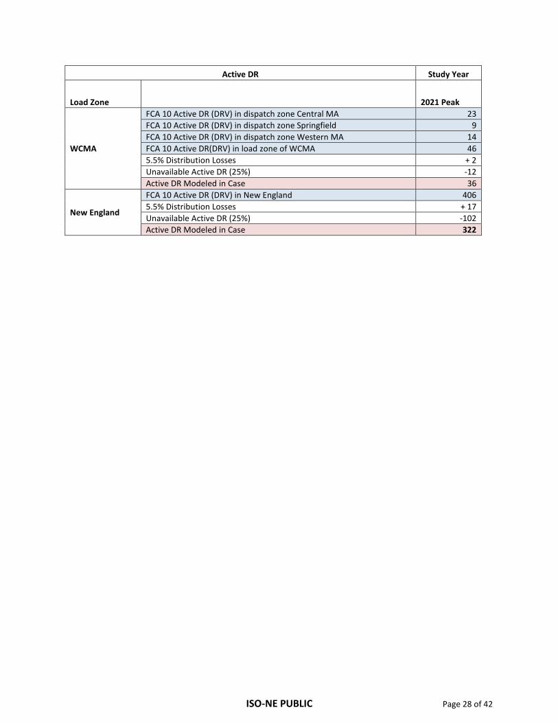
Active DR Study Year

Load Zone 2021 Peak

WCMA

FCA 10 Active DR (DRV) in dispatch zone Central MA 23 FCA 10 Active DR (DRV) in dispatch zone Springfield 9 FCA 10 Active DR (DRV) in dispatch zone Western MA 14 FCA 10 Active DR(DRV) in load zone of WCMA 46 5.5% Distribution Losses + 2 Unavailable Active DR (25%) -12 Active DR Modeled in Case 36

New England

FCA 10 Active DR (DRV) in New England 406 5.5% Distribution Losses + 17 Unavailable Active DR (25%) -102 Active DR Modeled in Case 322

ISO-NE PUBLIC Page 29 of 42

Section 4 Appendix C: PV generation Modeling As part of the final 2016 PV forecast the data on PV generation was divided into the following mutually exclusive categories:

• PV as a capacity resource in the Forward Capacity Market (FCM) • Non-FCM Settlement only Resources (SOR) and Generators (per OP-14) • Behind-the-Meter (BTM) PV (BTM)

The PV generation forecast only forecasts the PV values on a state-wide basis. However, within a state the PV does not grow uniformly, with some areas in the state having larger amounts of PV. To account for this locational variation of PV, the locational data of existing PV that is in-service as of the end of 2015 was utilized to obtain the percentage of PV that is in each dispatch zone. New England is divided into 19 dispatch zones and the percentage of PV in each dispatch zone as a percentage of total PV in the state is available. This percentage is assumed to stay constant for future years to allocate future PV to the dispatch zones. The percentage of existing solar in each dispatch zone as of the end of each year that is used as a part of the Solar PV forecast is based on Distribution Owner interconnection data and the materials are located at:

http://www.iso-ne.com/static-assets/documents/2016/04/2016_pvforecast_20160415.pdf

The distribution of existing PV resources by dispatch zone at the end of 2015 is provided in Table 18 below.

Table 18: Percentage of Installed PV in each state divided by Dispatch Zone as of 12/31/2015

State Dispatch Zone Name

Percentage of State PV in Dispatch Zone

Massachusetts

SEMA 21.50% Boston 10.90% Lower SEMA 18.70% Central MA 15.30% Springfield 6.00% North Shore 4.90% Western MA 22.70%

Connecticut

Eastern CT 18.80% Western CT 53.60% Northern CT 20.10% Norwalk-Stamford 7.50%

New Hampshire New Hampshire 88.30% Seacoast 11.70%

Vermont Northwest VT 62.90% Vermont 37.10%

Rhode Island Rhode Island 100.00%

ISO-NE PUBLIC Page 30 of 42

State Dispatch Zone Name

Percentage of State PV in Dispatch Zone

Maine Bangor Hydro 15.60% Maine 51.20% Portland 33.20%

Once the PV generation data is organized by dispatch zone, the PV within the dispatch zone falls into three categories:

• Category 1 : Units greater than 5MW: – Location data available – Will be modeled as an individual generators – 22.75 MW of PV in MA and 20 MW of PV in CT are the only resources that fall into this

category • Category 2 : Units greater than 1 MW and less than 5 MW

– Location data available through the PPA notifications – Needs to be modeled as injections at specific locations – Negative loads similar to DR

• Category 3: Units below 1 MW – No location data available – Needs to be modeled by spreading the MWs across the dispatch zone – Negative loads

similar to DR and spread across the load zone/dispatch zone like DR is spread

For PV in categories 2 and 3 the PV will be modeled as negative loads at the buses. The power factor of the negative load will be set to match the power factor of the load at the bus. If no load is present at the bus then a unity power factor will be assumed.

Based on a review of historic PV outputs, ISO-NE Transmission Planning has determined a 26% availability factor is applied to all categories of modeled PV generation in transmission planning studies.

The following table shows the PV generation modeled in the peak load case. Note that since the PV generation data is nameplate AC, a 5.5% gross up was performed to the PV generation forecast to account for avoided distribution losses.

Table 19: PV generation Modeled in the Peak Load Case

PV generation Modeled as Negative Loads Study Year

Load Zone 2021 Peak

Connecticut

PV generation (nameplate) in dispatch zone Eastern Connecticut 100 PV generation (nameplate) in dispatch zone Northern Connecticut 128 PV generation (nameplate) in dispatch zone Norwalk-Stamford 48 PV generation (nameplate) in dispatch zone Western 341

ISO-NE PUBLIC Page 31 of 42

PV generation Modeled as Negative Loads Study Year

Load Zone 2021 Peak

Connecticut A - Total PV generation (nameplate) in load zone of Connecticut 616 B - 5.5% Reduction in Distribution Losses 34

C - Unavailable PV generation (A+B)*(1-26%) 481 PV generation Modeled in Case as Negative Loads(A+B-C) 169

Maine

PV generation (nameplate) in dispatch zone Emera Maine 6 PV generation (nameplate) in dispatch zone Maine 20 PV generation (nameplate) in dispatch zone Portland ME 13 A - Total PV generation (nameplate) in load zone of Maine 39 B - 5.5% Reduction in Distribution Losses + 2 C - Unavailable PV generation (A+B)*(1-26%) -30 PV generation Modeled in Case as Negative Loads(A+B-C) 11

New Hampshire

PV generation (nameplate) in dispatch zone New Hampshire 53 PV generation (nameplate) in dispatch zone Seacoast 7 A - Total PV generation (nameplate) in load zone of New Hampshire 60 B - 5.5% Reduction in Distribution Losses + 3 C - Unavailable PV generation (A+B)*(1-26%) -47 PV generation Modeled in Case as Negative Loads(A+B-C) 17

Vermont

PV generation (nameplate) in dispatch zone Northwest Vermont 162 PV generation (nameplate) in dispatch zone Vermont 96 A - Total PV generation (nameplate) in load zone of Vermont 258 B - 5.5% Reduction in Distribution Losses + 14 C - Unavailable PV generation (A+B)*(1-26%) -202 PV generation Modeled in Case as Negative Loads(A+B-C) 71

Rhode Island

PV generation (nameplate) in dispatch zone Rhode Island 184 A - Total PV generation (nameplate) in load zone of Rhode Island 184 B - 5.5% Reduction in Distribution Losses + 10 C - Unavailable PV generation (A+B)*(1-26%) -144 PV generation Modeled in Case as Negative Loads(A+B-C) 51

NEMA/BOSTON

PV generation (nameplate) in dispatch zone Boston 157 PV generation (nameplate) in dispatch zone North shore 70 A - Total PV generation (nameplate) in load zone of NEMA/BOSTON 227 B - 5.5% Reduction in Distribution Losses + 12

ISO-NE PUBLIC Page 32 of 42

PV generation Modeled as Negative Loads Study Year

Load Zone 2021 Peak

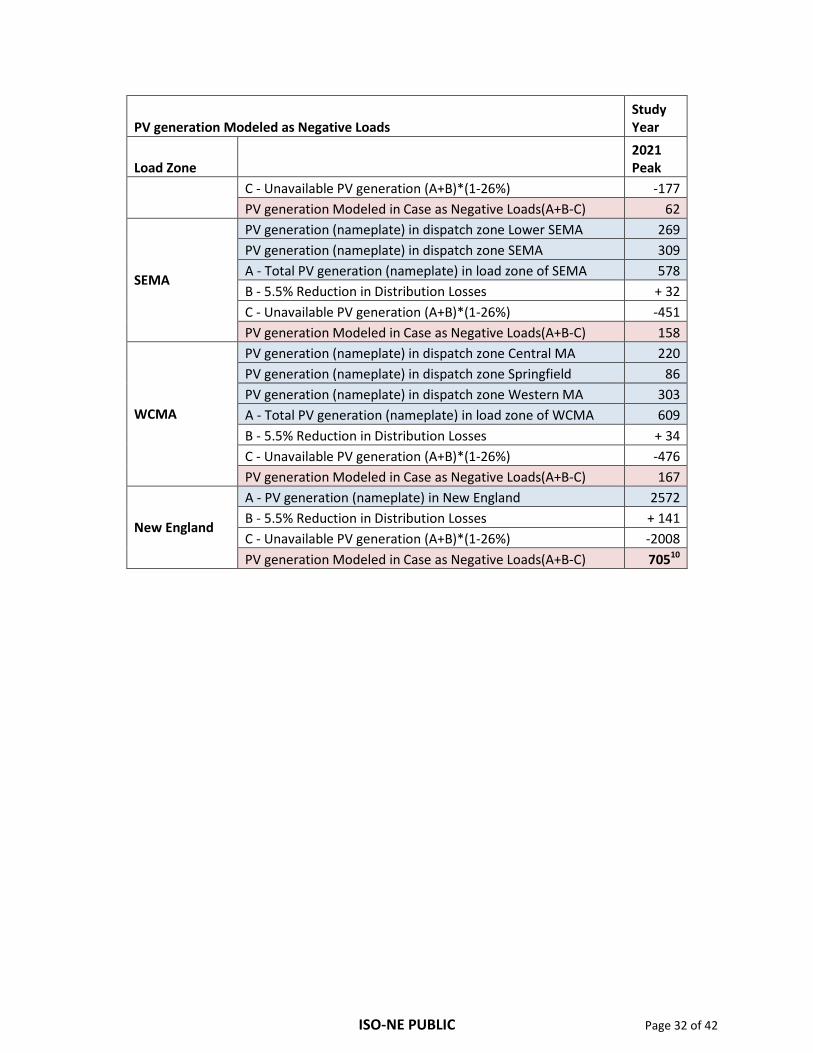
C - Unavailable PV generation (A+B)*(1-26%) -177 PV generation Modeled in Case as Negative Loads(A+B-C) 62

SEMA

PV generation (nameplate) in dispatch zone Lower SEMA 269 PV generation (nameplate) in dispatch zone SEMA 309 A - Total PV generation (nameplate) in load zone of SEMA 578 B - 5.5% Reduction in Distribution Losses + 32 C - Unavailable PV generation (A+B)*(1-26%) -451 PV generation Modeled in Case as Negative Loads(A+B-C) 158

WCMA

PV generation (nameplate) in dispatch zone Central MA 220 PV generation (nameplate) in dispatch zone Springfield 86 PV generation (nameplate) in dispatch zone Western MA 303 A - Total PV generation (nameplate) in load zone of WCMA 609 B - 5.5% Reduction in Distribution Losses + 34 C - Unavailable PV generation (A+B)*(1-26%) -476 PV generation Modeled in Case as Negative Loads(A+B-C) 167

New England

A - PV generation (nameplate) in New England 2572 B - 5.5% Reduction in Distribution Losses + 141 C - Unavailable PV generation (A+B)*(1-26%) -2008 PV generation Modeled in Case as Negative Loads(A+B-C) 70510

ISO-NE PUBLIC Page 33 of 42

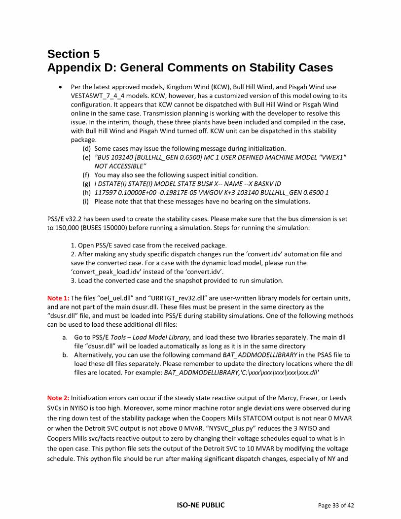
Section 5 Appendix D: General Comments on Stability Cases

• Per the latest approved models, Kingdom Wind (KCW), Bull Hill Wind, and Pisgah Wind use VESTASWT_7_4_4 models. KCW, however, has a customized version of this model owing to its configuration. It appears that KCW cannot be dispatched with Bull Hill Wind or Pisgah Wind online in the same case. Transmission planning is working with the developer to resolve this issue. In the interim, though, these three plants have been included and compiled in the case, with Bull Hill Wind and Pisgah Wind turned off. KCW unit can be dispatched in this stability package.

(d) Some cases may issue the following message during initialization. (e) “BUS 103140 [BULLHLL_GEN 0.6500] MC 1 USER DEFINED MACHINE MODEL "VWEX1"

NOT ACCESSIBLE” (f) You may also see the following suspect initial condition. (g) I DSTATE(I) STATE(I) MODEL STATE BUS# X-- NAME --X BASKV ID (h) 117597 0.10000E+00 -0.19817E-05 VWGOV K+3 103140 BULLHLL_GEN 0.6500 1 (i) Please note that that these messages have no bearing on the simulations.

PSS/E v32.2 has been used to create the stability cases. Please make sure that the bus dimension is set to 150,000 (BUSES 150000) before running a simulation. Steps for running the simulation:

1. Open PSS/E saved case from the received package. 2. After making any study specific dispatch changes run the ‘convert.idv’ automation file and save the converted case. For a case with the dynamic load model, please run the ‘convert_peak_load.idv’ instead of the ‘convert.idv’. 3. Load the converted case and the snapshot provided to run simulation.

Note 1: The files “oel_uel.dll” and “URRTGT_rev32.dll” are user-written library models for certain units, and are not part of the main dsusr.dll. These files must be present in the same directory as the “dsusr.dll” file, and must be loaded into PSS/E during stability simulations. One of the following methods can be used to load these additional dll files:

a. Go to PSS/E Tools – Load Model Library, and load these two libraries separately. The main dll file “dsusr.dll” will be loaded automatically as long as it is in the same directory

b. Alternatively, you can use the following command BAT_ADDMODELLIBRARY in the PSAS file to load these dll files separately. Please remember to update the directory locations where the dll files are located. For example: BAT_ADDMODELLIBRARY,'C:\xxx\xxx\xxx\xxx\xxx.dll'

Note 2: Initialization errors can occur if the steady state reactive output of the Marcy, Fraser, or Leeds SVCs in NYISO is too high. Moreover, some minor machine rotor angle deviations were observed during the ring down test of the stability package when the Coopers Mills STATCOM output is not near 0 MVAR or when the Detroit SVC output is not above 0 MVAR. “NYSVC_plus.py” reduces the 3 NYISO and Coopers Mills svc/facts reactive output to zero by changing their voltage schedules equal to what is in the open case. This python file sets the output of the Detroit SVC to 10 MVAR by modifying the voltage schedule. This python file should be run after making significant dispatch changes, especially of NY and

ISO-NE PUBLIC Page 34 of 42

ME machines. Note that this python file solves the case with the following solution options: transformers regulating, switched shunts regulating, phase angle regulators regulating, and area interchange enabled. If different solution options are used then the python file will need to be modified accordingly.

Note 3: The file “V82BCPMX1.DAT,” must be present in the same directory as the DSUSR.dll, otherwise PSS/E dynamics crashes. This file links to certain Vestas wind farm models.

Note 4: The file “CP_GW90.txt” must be included in same directory as all other data in order for Georgia Mountain Wind user model to function correctly.

Note 5: With the inclusion of the 326 SPS thermal mode relay model, to use this model when simulating with faults that include opening Line 326, a small value of shunt MVA (1-j1) is needed on either the Scobie Pond or Lawrence Road 345-kV buses and the Scobie Pond-Lawrence Road section of Line 326 needs to stay in-service. This allows a negligible MVA to still be flowing on Scobie Pond-Lawrence Road section of Line 326, otherwise the model will trip the assigned branches (generator GSUs), even though the thermal set point may not have been reached. Opening of the Scobie Pond-Lawrence Road section of Line 326, which is being monitored by the SPS model, causes the assigned branches to be tripped (and thereby tripping the units associated with this SPS) after the associated time delay; this is inherent in the PSSE relay model.

Note 6: The voltage sag model is meant to track voltage dips that would occur after the fault clears and the voltage has recovered. There is a rare chance for false positives based on the existing version of the model in the dynamics cases. For a majority of simulations, the false positive would not show up since it requires that the voltage at buses during a fault vary in a manner that it could look like the fault cleared. The ‘VDYSA4’ model allows the user to set a constant “FLAGG” during the dynamic simulation to indicate that the fault is still being applied. This prevents the model from reporting any voltage sag violations during the fault. This is an optional parameter that may be used during the simulation if the user is concerned with false positives. Engineering judgement may be used to determine if this is necessary for a particular fault that is being simulated. CON “FFLAG” is set to a default value of 0.0 in the stability snapshots and it will behave like the original voltage sag model even if the user did not set this parameter. To enable the new functionality, the user can set the CON “FFLAG” to 1.0 before applying a fault and should reset it to 0.0 after removing the fault. While the CON “FFLAG” is 1.0, the voltage sag delay and low limit failures are suppressed.

Note 7: Note that the following special protection systems (SPSs) are hard-coded in the stability snapshots and some changes made to these models are noted in the “readme.txt” file in each stability package:

• 345 kV line 396 SPS model • 345 kV line 326 SPS stability mode model • Dedicated Path Logic (DPL) SPS model • Maine capacitor tripping models

ISO-NE PUBLIC Page 35 of 42

Note 7: Note that if the 60 Second Disturbance Simulation as described in the MMWG model manual15 is performed on the posted basecase with the Millstone 3 generator online, the prescribed requirement of generator MW deviation of less than 1 MW will not be met. This is consistent with the plant characteristics data as submitted by the plant owner.

15 https://rfirst.org/reliability/easterninterconnectionreliabilityassessmentgroup/mmwg/Documents/MMWG_Procedure_Manual_V14.pdf

ISO-NE PUBLIC Page 36 of 42

Section 6 Appendix E: PSS/E Voltage Sag User Model VDYSA4

November 16, 2007, Revised February 5, 20081, Revised September 1, 20152, Revised May 1, 20163

VDYSA4 is a Bus Voltage Monitoring Model

Model VDYSA4 is a voltage monitoring PSS/E user model designed to check New England area (101) bus voltages against a set of voltage parameters. The model currently allows for up to 5000 buses. The New England Area number, 101, and the allowable bus number of 5000 are both hard coded in the program. The model user sets three different voltage sag parameters (CONS), an upper voltage limit, a lower voltage limit (creating a voltage dip range), and a voltage sag recovery time limit.

1Newly added to the VDYSA2 model is a voltage recovery subroutine. The model user sets three different parameters for this subroutine, a voltage drop set point to start monitoring a bus voltage recovery, a voltage recovered set point, and a voltage recovery time limit.

2An additional CON has been added to the model to disable the voltage sag calculation during the fault. Model was also corrected so that when a bus is out of service, it is excluded from all reporting.

3Additional CONs have been added to the model to allow two voltage recoveries and the fault flag was changed to an ICON.

DYRE File

Ten data entries, CONS, are required for the model in the DYR file:

0 'USRMDL' 0 'VDYSA4' 8 0 1 9 0 0 FFLAG AAA BBB CCC DDD EEE FFF GGG HHH III JJJ/

0

0 'USRMDL' 0 'VDYSA4' 8 0 1 9 0 0 0 0.70 0.80 0.25 69 0.75 0.80 0.50 0.80 0.85 0.60/

0

What the model CONS are:

AAA is the V-Sag voltage range low limit set point in Vpu (0.70 Vpu),

ISO-NE PUBLIC Page 37 of 42

BBB is the V-Sag voltage range upper limit set point in Vpu (0.80 Vpu),

CCC is the V-Sag voltage sag time allowed in seconds (0.25 seconds),

DDD is the minimum bus voltage level to monitor in kV (i.e. 69 kV and above)

EEE: is the first voltage drop set point to start monitoring for voltage recovery in per unit (0.75 Vpu)

FFF: is the voltage recovery set point in per unit (0.80 Vpu)

GGG: is the voltage recovery time allowed in seconds (0.50 seconds)

HHH: is the second voltage drop set point to start monitoring for voltage recovery in per unit (0.80 Vpu)

III: is a second voltage recovery set point in per unit (0.85 Vpu)

JJJ: is a second voltage recovery time allowed in seconds (0.60 seconds)

The model ICON FFLAG: is the flag indicating system is faulted (0 no fault active, 1 fault applied)

CON AAA must be set less than CON BBB, or else the VDYSA3 model is ignored and the message reported is: VDYSAG MODEL IGNORED: V-SAG RANGE LOWER SETPOINT V= AAA IS GREATER THAN UPPER SETPOINT V= BBB.

CON EEE must be set less than CON FFF, or else the VDYSA3 model is ignored and the message reported is: VDYSAG MODEL IGNORED: V-DROP SETPOINT V= EEE IS GREATER THAN V-RECOVERY SETPOINT V= FFF.

ICON FFLAG should normally be set to a value of 0. The user can set this model to 1 when applying a fault and should reset it to 0 when removing the fault. While FFLAG is 1, the voltage sag delay and low limit failures are suppressed.

The voltage sag subroutine ignores the initial voltage drop below 0.80 Vpu and monitors for voltage rise to 0.80. At this point, if the voltage drops below 0.80 Vpu again, then the voltage sag subroutine timer starts (0.25 seconds). Should the voltage remain between 0.80 – 0.70 Vpu for longer than the allotted voltage sag time, 0.25 seconds in this case, then a “V-Sag Time Delay Failure” message is reported. Should the voltage rise above 0.80 Vpu before the voltage sag timer times out, then the timer is reset and that bus continues to be monitored for voltage sag. Should the bus voltage drop below 0.70 Vpu before the V-Sag timer times out (0.25 seconds), then a “V-Sag Low Limit Failure” message is reported.

ISO-NE PUBLIC Page 38 of 42

Once a particular bus has been reported on for a voltage sag time delay failure, then that particular bus will no longer be reported on for that type of failure. The same methodology applies to the voltage sag low limit failure.

The voltage not recovered subroutine does not ignore the initial voltage drop. If at any time the voltage drops below the first recovery voltage subroutine set point of 0.75 Vpu then does not rise above the voltage recovery set-point of 0.80 Vpu in the allotted voltage recovery time specified, 0.50 seconds in this case, then a “Voltage Not Above V1= * message is reported. Where * is the recovery voltage set point. A second set of parameters are provided to model a second recovery. NOTE THAT ONLY ONE MODEL OF THIS TYPE IS ALLOWED in a dynamic stability setup. The user should remove the VDYSAG model if this new revised model is added..

ISO-NE PUBLIC Page 39 of 42

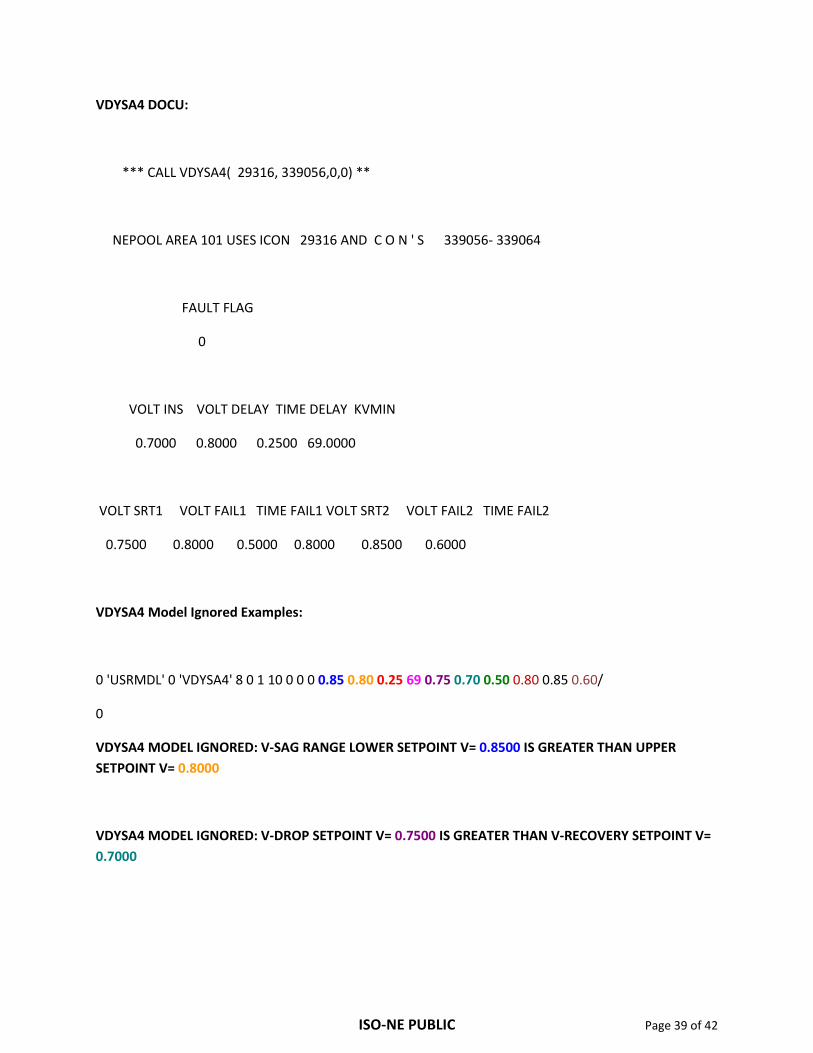
VDYSA4 DOCU:

*** CALL VDYSA4( 29316, 339056,0,0) **

NEPOOL AREA 101 USES ICON 29316 AND C O N ' S 339056- 339064

FAULT FLAG

0

VOLT INS VOLT DELAY TIME DELAY KVMIN

0.7000 0.8000 0.2500 69.0000

VOLT SRT1 VOLT FAIL1 TIME FAIL1 VOLT SRT2 VOLT FAIL2 TIME FAIL2

0.7500 0.8000 0.5000 0.8000 0.8500 0.6000

VDYSA4 Model Ignored Examples:

0 'USRMDL' 0 'VDYSA4' 8 0 1 10 0 0 0 0.85 0.80 0.25 69 0.75 0.70 0.50 0.80 0.85 0.60/

0

VDYSA4 MODEL IGNORED: V-SAG RANGE LOWER SETPOINT V= 0.8500 IS GREATER THAN UPPER SETPOINT V= 0.8000

VDYSA4 MODEL IGNORED: V-DROP SETPOINT V= 0.7500 IS GREATER THAN V-RECOVERY SETPOINT V= 0.7000

ISO-NE PUBLIC Page 40 of 42

Dynamic Voltage Sag Model VDYSA4

Voltage Sag Subroutine

V-Sag Time Delay Failure

0.80

0.70

Voltage Sag Subroutine Initial Voltage Dip Ignored

Voltage Sag Subroutine Voltage Recovers Monitoring For Next Sag

Voltage Sag Subroutine Timer Starts

0.25 s

Voltage Sag Subroutine Timer Stops

Voltage Sag Subroutine Voltage Range Upper Limit

Voltage Sag Subroutine V-Sag Time Delay Failure Message Triggered

Bus Voltage (pu)

Time (s)

Figure 1 - Dynamic Voltage Sag Model

Voltage Sag Subroutine Voltage Range Low Limit

ISO-NE PUBLIC Page 41 of 42

Dynamic Voltage Sag Model VDYSA4

Voltage Sag Subroutine

V-Sag Low Limit Failure

0.80

0.70

Voltage Sag Subroutine Initial Voltage Dip Ignored

Voltage Sag Subroutine Voltage Recovers Monitoring for Next Sag

Voltage Sag Subroutine Timer Starts

0.25 s

Voltage Sag Subroutine Voltage Range Low Limit

Voltage Sag Subroutine Timer Stops

Voltage Sag Subroutine V-Sag Low Limit Failure Message Triggered

Time (s)

Figure 2 - Dynamic Voltage Sag Model

Voltage Sag Subroutine Voltage Range Upper Limit

Bus Voltage (pu)

Page 42 of 42 ISO-NE PUBLIC

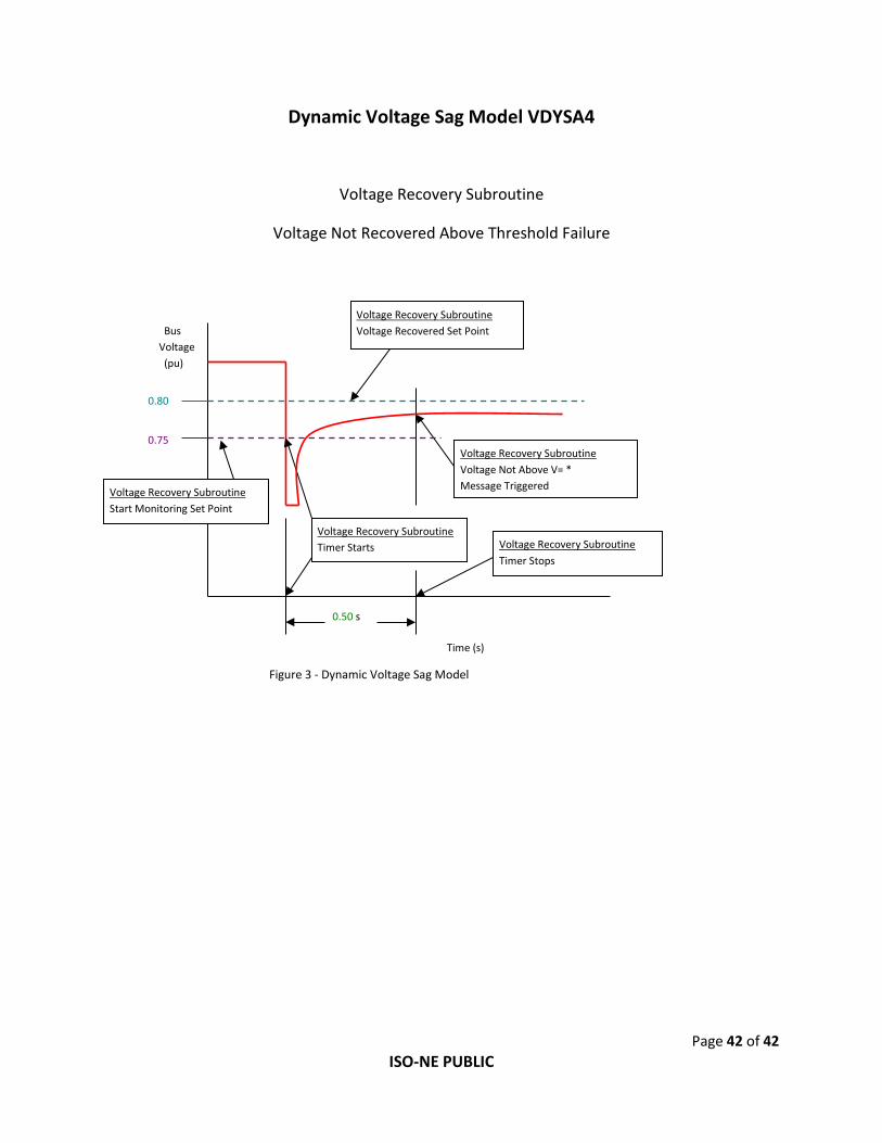
Dynamic Voltage Sag Model VDYSA4

Voltage Recovery Subroutine

Voltage Not Recovered Above Threshold Failure

0.75

Voltage Recovery Subroutine Timer Starts

Voltage Recovery Subroutine Voltage Recovered Set Point

0.50 s

Voltage Recovery Subroutine Start Monitoring Set Point

Time (s)

Bus Voltage (pu)

Voltage Recovery Subroutine Voltage Not Above V= * Message Triggered

Voltage Recovery Subroutine Timer Stops

Figure 3 - Dynamic Voltage Sag Model

0.80