seasonal characteristics of two saline lakes in washington

Seasonal Characteristics of Two Saline Lakes in WashingtonAuthor(s): G. C. AndersonSource: Limnology and Oceanography, Vol. 3, No. 1 (Jan., 1958), pp. 51-68Published by: American Society of Limnology and OceanographyStable URL: http://www.jstor.org/stable/2832592 .

Accessed: 17/06/2014 22:43

Your use of the JSTOR archive indicates your acceptance of the Terms & Conditions of Use, available at .http://www.jstor.org/page/info/about/policies/terms.jsp

.JSTOR is a not-for-profit service that helps scholars, researchers, and students discover, use, and build upon a wide range ofcontent in a trusted digital archive. We use information technology and tools to increase productivity and facilitate new formsof scholarship. For more information about JSTOR, please contact [email protected].

.

American Society of Limnology and Oceanography is collaborating with JSTOR to digitize, preserve andextend access to Limnology and Oceanography.

http://www.jstor.org

This content downloaded from 195.78.108.81 on Tue, 17 Jun 2014 22:43:34 PMAll use subject to JSTOR Terms and Conditions

http://www.jstor.org/action/showPublisher?publisherCode=limnoc

http://www.jstor.org/stable/2832592?origin=JSTOR-pdf

http://www.jstor.org/page/info/about/policies/terms.jsp


Seasonal Characteristics of Two Saline Lakes in Washington

G. C. ANDERSON

Department of Zoology, University of Washington, Seattle

ABSTRACT

The limnology of two highly saline lakes in Washington was studied in relation to the physical and chemical conditions which influence the growth and distribution of phytoplankton. The lakes were sampled at frequent intervals for a period of more than a year in 1950 and 1951. Morphometric conditions were determined, and routine sampling in- cluded measurements of temperature, transparency, oxygen, pH, alkalinity, phosphate, chlorophyll, and quantitative samples of phytoplankton. Lake Lenore, the less saline of the two (T.D.S. 14 g/liter), is shallow and was unstratified during the investigation. Dis- solved nutrients were high and showed erratic variations during the summer. The phytoplankton population was taxonomically simple and was made up mainly of two species of diatoms-Amphora sp. which formed the spring bloom, and Chaetoceros elmorei which made up the late summer bloom. Soap Lake is relatively deep, meromictic, and saline (T.D.S. 35 g/liter). Temperature conditions were dichothermic, and the nutrient content was high, especially in the monimolimnion. A winter maximum and a summer minimum was observed in the phytoplankton population, and a change in the biota has been noted during dilution of the lake in recent years. Indication of grazing by zooplankton was found in both lakes.

INTRODUCTION

Seasonal information on saline, desert lakes is rather meager, and apart from the work contributed by Young (1924) in Devils Lake, by Hutchinson (1937) on lakes in Nevada, and by Rawson and Moore (1944) on Saskatchewan lakes, little is known of these lakes in North America. Most lim- nological work in arid regions has been carried out by expeditions to places that are not readily accessible. Due to time limita- tions, little has been learned of seasonal events, and hence comparison with other types of lakes intensively studied has been superficial. The present paper is confined to seasonal fluctuations of physico-chemical factors and of the phytoplankton populations.

There are many lakes of varying degrees of salinity in the easily accessible Columbia Basin of Central Washington, and for the present study, two of the more saline lakes were chosen for the study of seasonal events. Soap Lake is the terminal one in a chain of lakes which lie in the old river bed of the Columbia River in the Lower Grand Coulee. Lake Lenore lies to the north. The Grand Coulee is a basalt canyon formed by the flow of the Columbia River during glacial

times. Upon disappearance of the ice, the river returned to its former drainage system, the present location of the Columbia River, and the Grand Coulee became dry except for the chain of lakes now present (Bretz 1932).

Both Soap Lake and Lake Lenore are highly alkaline, the waters of which are composed chiefly of the sodium salts of sulfate, bicarbonate, carbonate, and chloride (Table 1). A seepage inlet at the north end of Lake Lenore supplies water from the relatively fresh but hardwater lakes lying in the northern section of the Lower Grand Coulee. Lake Lenore has no outlet, however, and Soap Lake has neither a surface inlet nor outlet. It is believed that an underground connection is present between the two lakes, but the significance of this is not known (Mundorff and Bodhaine 1954). It becomes apparent from this that the salt content of the lakes is due to the absence of outlets. A gain of water occurs by drainage from the surrounding cliffs and plateaus especially during the spring runoff, and loss of water takes place chiefly by evaporation. For this reason the salt content has increased since the origin of the lakes. In recent years, there has been a

51



52 G. C. ANDERSON

TABLE 1. Mineral analyses of the surface waters of Soap Lake and Lake Lenore, November 1950

(mg/liter) Analyses by United States Bureau of

Reclamation, Denver, Colorado

Soap Lake Lake Lenore

Total solids 35280 14080 Calcium 20.6 10.2 Magnesium 8.2 13.8 Sodium 11868 5129 Potassium 1134 437.9 Carbonate 6870 3000 Bicarbonate 5209 3544 Sulfate 6240 2112 Chloride 5467 1438 Nitrate 8.7 8.7

substantial additional flow of water into Soap Lake, which has been ascribed collec- tively to increased precipitation, rise in ground water level, and irrigation canal leakage. Pumps have been installed by the U. S. Bureau of Reclamation on both lakes to remove the excess water, and as a result the lakes have suffered a considerable decrease in salinity.

Lake Lenore is an elongate shallow body of water. Summer stratification is weak and transitory due to the shallow depth and mixing by wind. The bottom of the lake is rocky for the most part, and aquatic plants around the shore are sparse. Some saltgrass (Distichlis stricta) and Nevada club-rush (Scirpus nevadensis) have been reported (Scheffer 1946).

Soap Lake is a meromictic lake. Autumn and spring circulation followed by summer thermal stratification occurs in the upper part of the lake (mixolimnion), but the bottom layer (monimolimnion) never becomes mixed with the upper waters. The bottom layer is composed of a dense yellow- ish-brown water which contained more than four times the concentration of salts of the upper waters in 1950. The odor of hydrogen sulfide is strong in the bottom water and in the black organic deposits which make up the bottom of the lake. There was no evidence of animal life in these deposits. The aquatic plant population of the littoral zone is scant and consists entirely of emer- gent forms (Scheffer 1946). Saltgrass (Dis- tichlis stricta), Nevada club-rush (Scirpus

nevadensis), and common toad rush (Juncus bufonius) were present.

The writer is indebted to Dr. W. T. Edmondson for constant encouragement and direction during the period of the study and for valuable criticism and advice during the preparation of the manuscript. Thanks are due to Dr. G. W. Comita for collaboration in the field work and for permission to use data from his analyses of 02, pH, and alkalinity. Dr. R. Thompson of the Univer- sity of Kansas, Dr. R. Patrick of the Acad- emy of Natural Sciences of Philadelphia, Dr. F. Drouet of the Chicago Museum of Natural History, and Mr. H. E. Sovereign aided in the identification of the phytoplankters. Personnel of the U. S. Bureau of Reclamation at Ephrata, Washington, made available all of their information on these lakes in the form of topographic maps, aerial photographs, chemical analyses, and lake level fluctuations. Financial support and equipment supplied by the Department of Zoology and from Initiative-171 funds of the State of Washington are gratefully acknowledged.

MATERIALS AND METHODS

In each lake a single station was established for all routine sampling. In Soap Lake, the station was in the region of maximum depth. Two locations deeper than the station selected were present in Lake Lenore, but both appeared to be atypical of the lake as a whole.

Morphometric data for Lake Lenore were obtained by sounding with a brass chain. Depth contours were added to an outline map of Lake Lenore taken from the U. S. Bureau of Reclamation, Columbia Basin topographic chart 222-P-5529. Morpho- metric data for Soap Lake were obtained from the U. S. Bureau of Reclamation, Soap Lake topographic map 222-116-25067.

Sampling of the lakes was carried out at different time intervals depending upon the season of year. During the winter, sampling was done every three to four weeks, while during the period of stratification samples were taken every two weeks as far as was possible.

Water samples were usually collected at



TWO SALINE LAKES IN WASHINGTON 53

the surface, middle, and bottom of the lakes. This procedure was occasionally modified to suit the existing conditions. At each depth four liters of water were collected in either a two-liter or a four-liter Kemmerer water bottle, drained into glass gallon jugs, and brought back to the laboratory in this con- dition. From the water in these jugs the various chemical determinations were made and phytoplankton samples taken. Before the water was drained from the sampling bottle into the jugs a sample of water was taken in a 250 cc reagent bottle for the determination of dissolved oxygen. An attempt was made to do the water analyses as soon as possible after the return to the laboratory from the lake. The time before analyses was sometimes quite long due to the distance of the lakes from the laboratory. In some instances the samples were analysed within eight to ten hours after taking and in other instances the samples were left over- night, in which case they were stored in a coldroom at a temperature of 100C.

The surface temperature of the lake and the air temperature were measured with a laboratory thermometer graduated in degrees Centigrade. A temperature profile of the entire depth of the lake was obtained with a bathythermograph.

The transparency of the lakes was measured with a fully white, 20 cm diameter Secchi disc.

A plankton sample for qualitative pur- poses was taken with a fine-mesh, usually number 25 bolting silk, plankton net. A vertical tow from about five meters depth was the usual procedure. The sample was preserved in approximately 4 per cent formalin.

Dissolved oxygen was determined by the unmodified Winkler method (American Public Health Association 1946). The manganous sulfate, alkaline iodide, and sulfuric acid reagents were added im- mediately after the sample was taken, and the titration was carried out at the laboratory. Large amounts of acid were needed to neutralize the samples, and because a standard amount was not added each time, corrections were not made for the volume of reagents introduced. With the addition

of acid, a violent bubbling took place due to the high carbonate content. Because of these difficulties the oxygen values are open to question.

The hydrogen ion concentration was measured with a Beckman pH meter. Alkalinity was determined by titrating 10-ml samples of lake water with 0.5N sulfuric acid to the phenolphthalein and methyl orange endpoints. Differentiations of the alkalinities due to hydroxide, normal carbonate, and bicarbonate was done according to the American Public Health Association (1946, Table 4, page 9). The results are expressed as mg/liter C03= and HCO3-. Small quantities of hydroxide were recorded infrequently, the significance of which is not known, but may have been due to technical error.

Phosphate concentration was determined by the method described by Robinson and Thompson (1948). Standards were not run with every series of determinations, but repeated calibrations showed that under the conditions used, the variation was un- important. The method was modified somewhat because of the alkalinity of the lakes. One ml of concentrated sulfuric acid was added before the addition of reagents to lower the pH to 4.2, the point of maximum color development. It was sub- sequently found that dilution of the samples was necessary to give true values, and corrections were applied to all the data in this respect. The presence of possible interfer- ing substances in the monimolimnion of Soap Lake make those values questionable.

Nitrate determinations were attempted with the strychnidine method (Zwicker and Robinson 1944), but it was found that variability was great and standard amounts added to lake water could not be recovered with any degree of precision. Evidently the strychnidine reagent does not work in highly alkaline waters, and hence special methods will have to be developed for these lakes.

Chlorophyll determinations were made according to the method outlined by Edmond- son and Edmondson (1947). One liter of water, or less, depending upon the quantity of plankton present, was filtered through



54 G. C. ANDERSON

Schleicher and Schuell number 576 ana- lytical filter paper. The entire filter paper was ground with purified sand in a mortar with 80 per cent acetone. The mortar was allowed to stand at least 15 minutes in the dark, after which time it was filtered through a sintered glass filter into Klett tubes. The filtrate was made up to 10 ml and then read in the Klett colorimeter using filter K66. Edmondson and Edmondson (1947) have shown that the K66 filter adequately measures chlorophyll a with a possibility of interference from chlorophyll b and chloro- fucin.

Phytoplankton samples were prepared by centrifuging 50-ml samples of water in a clinical centrifuge at a speed of approximately 1500 rev/min for 10 minutes. The water was drawn off carefully so that only 1 or 2 ml remained. The remaining solution was thoroughly mixed and transferred to a vial where it was fixed in Transeau's solution (6 parts water, 3 parts 95 per cent alcohol, 1 part formalin). It was found that when samples were mounted on a slide with cover glass, a violent swirling took place which made it impossible to count accurately. This was overcome by increas- ing the viscosity of the solution with the addition of a few drops of glycerine to each sample. The samples were counted using a method similar to that described by Lackey (1938).

The volume of each species was calculated. The necessary measurements were made with the use of an ocular micrometer, and, by the application of formulae for the volumes of bodies which the species most nearly represented in shape, the volumes were estimated. In this manner the total volume of phytoplankton was calculated.

LAKE LENORE

Morphometry Lake Lenore is elongate, with a length

of 9.2 km and a maximum width of 0.9 km. The maximum depth is 11 m and the mean depth is 6.5 m. Details of the morphometry are given in Table 2.

Physical and chemical conditions Temperature. Thermal stratification in

Lake Lenore was at most times absent

TABLE 2. Morphometric features of Lake Lenore

Depth (m) Area (ha) Volume (ms)

0 556 5,408,000

1 526 10,128,000

3 487 9,196,000

5 433 7,207,000

7 292 3,468,000

9 78 640,000

11 3

Total 36,042,000 Mean depth 6.5 m Maximum depth 11.0 m

(Fig. 1). With the disappearance of the ice cover in late February the lake was homothermal at approximately 0?C. During the period of spring heating, a temperature gradient was established and was most pronounced in the middle of May with a surface temperature of 14.2?C and a bottom temperature of 5.6?C. After this, the temperature gradient was gradually reduced, and by the end of July the entire lake was homothermal at 22?C. The lake remained homothermal until the appearance of an ice cover in January, 1951.

The annual heat budget was 16,110 g-cal/cm2 of lake surface. The period of heating used for the calculation was the minimum weighted mean winter temperature of -0.49?C on February 18, 1950, to the maximum weighted mean summer temperature of 22.2?C on August 27, 1950. The heat budget for Lake Lenore is of limited value and is not comparable with those of large, deep lakes. Because the top and bottom waters attain the same maximum temperature, there must be much heat lost to the bottom mud which would therefore render the value of the heat budget minimal in comparison with other lakes.

Transparency. The range of transparency was large (Fig. 1), from a minimum of 1 m on March 26, 1950, a period when the water was turbid due to spring inflow from the melting snow of the surrounding cliffs, to a maximum of 8.5 m in midsummer and




0 0 Nv-t'IO 'IO t 0 N N W'O -4 0 co O'- N 0 O > 4 <X -, :

. - O Cg N (M 1-4:

350

1.0 _ X

0

5

90

@1

h 8

4 0 M./_~ ~10X

w 19504 M.-

FIG 1. SesnlvrainMftmeatr,tasaec,dsovd.xgn laiiy n h

0 5 a.

0~~~~~~~~~~~~~~~~~~~

* 3~ ~ ~ ~ ~ ~~~~~~~~~~0

>_ 29C 3 900

aveage fo h ntr ae

z E 0

4j P944-

0 M A M J J A S 0 N D J F

1950 19951 FIG. 1. Seasonal variations of temperature, transparency, dissolved oxygen, alkalinity, and phos-

phate in Lake Lenore, February 1950 to February 1951. Alkalinity and phosphate values are weighted averages for the entire lake.

autumn. The arithmetic average for the year was 4.4 m.

Dissolved oxygen. As would be expected because of the limited thermal stratification,

there was likewise a limited stratification of dissolved oxygen (Fig. 1). The period of maximum oxygen stratification was in June which coincided with the maximum thermal



56 G. C. ANDERSON

gradient. The oxygen concentration in the bottom waters reached a minimum of 0.9 mg/liter on June 15 but increased shortly after this due to the mixing of the entire lake. There was a sudden drop in oxygen concentration at all levels on September 23 which, as will be discussed later, coincided with a sudden almost complete disappearance of the phytoplankton population. This was followed by a rise in concentration and maintenance of a constant oxygen concentration throughout the winter. There was another slight increase in Febru- ary, 1951.

It is difficult to form an idea of the trophic nature of Lake Lenore from the oxygen conditions. Calculation of the hypolim- netic oxygen deficit is not possible because stratification was not established.

Hydrogen ion concentration. There was little vertical or seasonal variation of the pH in Lake Lenore. A minimum of pH 9.69 was observed in the 4 to 8 m depth zone on June 15, 1950, and a maximum of pH 10.02 was obtained at the surface on April 22, 1950. This small range of pH demonstrates the highly buffered nature of the water.

Alkalinity. The alkalinity of Lake Le- nore is made up of two fractions, bicarbonate and carbonate. There was little vertical stratification of the alkalinity so that the weighted averages of all the depth zones of the bicarbonate and carbonate illustrate adequately the seasonal fluctuations (Fig. 1).

The bicarbonate was at most times in lower concentration than the carbonate. There was a reduction to zero of the bicarbonate in the spring, which was followed by a rise and then a fairly steady state of approximately 1000 mg HCO3-/liter throughout the summer and fall. During the winter there was a further increase to 2500 mg HCOj-/liter.

The carbonate remained high at all times. A drop to 2800 mg C03=/liter in May, and an increase to 5200 mg/liter in October followed by a gradual decrease during the winter were the salient features of the seasonal carbonate cycle. There were times when a decrease in the bicarbonate concentration was accompanied by an increase in

the carbonate concentration. This is probably a result of the conversion of bicarbonate to carbonate due to the removal of CO2 by photosynthesis.

Phosphate. There was little vertical stratification of the phosphate so that only the weighted average of all depths is illus- trated (Fig. 1). The phosphate concentration was very high in early spring (195 ,ug-atoms/liter) but decreased rapidly almost to zero in May. This was followed by a rise in June and a further decrease to almost zero in July and August. Toward the end of August an increase of short duration occurred. During the remainder of the study, the phosphate concentration fluctuated slightly around 20 ,ug-atoms/liter. On only one date, June 15, was there considerable vertical stratification, with a minimum of 2.8 ,ug-atoms/liter at the top and 141.6 at the bottom. Thus, chemical stratification coincided with the period of the maximum thermal gradient. It was not possible to calculate the rate of phosphate accumulation in the bottom waters because of complete mixing after June 15.

The great fluctuations in phosphate concentration indicate either a high phytoplankton production or a storage of phosphate by phytoplankters in excess of that required for growth or possibly a combina- tion of the two. Nitzschia and Chlorella (Ketchum 1939, Scott 1945) can store phosphorus in excess of immediate require- ments, and the same phenomenon has been shown for Asterionella (Lund 1950). Ein- sele (1941) described the storage of large quantities of phosphate by the Schleinsee phytoplankton with no increase in the population.

Phytoplankton The phytoplankton of Lake Lenore is

taxonomically simple in regard to numbers of species present (Table 3): 15 genera, 18 species, and 2 miscellaneous categories occurred. One miscellaneous group is composed of small blue-green and green algae, the other is composed of diatoms.

The three indices of the standing crop- chlorophyll concentration, cell number, and cell volume showed the same general seasonal trends, although the magnitude of



TABLE 3. Volume calculations of the seasonal and vertical distribution of the species of phytoplankte?s in Lake Lenore, March 1950 to February 1961

For each species and date the upper figure represents volume at 0 m, middle-4 m, and lower-8 m. Multiply the values shown by 1O3 to get /A3/ml.

1950 1951

Mar. Apr. Apr. May June July July Aug. Aug. Sept. Sept. Oct. Nov. Nov. Dec. Jan. Feb. 4 8 22 20 15 15 29 12 25 8 23 14 4 24 16 20 17

Chrysophyta Asterionella 10.8 6.7

formosa 8.7 4.0 1.3 7.4 2.0 1.3 2.0 35.7 26.9 1.3

Chaetoceros 43.6 15.0 213.7 694.1 28.6 4 1 8.2 6.8 elmorei (vege- 35.4 34.0 183.7 295.3 13.6 8.2 tative cells) 16.0 61.2 530.8 458.7 9.6 12.2 13.6 10.9 12.2

Chaetoceros 46.8 54.9 42.0 4.1 8.8 31.2 5.4 43.4 elmorei (stat- 1.4 116.6 15.6 158.7 5.4 8.8 22.4 25.8 45.4 10.8 ospores) 71.2 118.6 1.4 27.1 36.6 16.9 87.5

Cyclotella 2.4 12.1 17.0 36.3 4.8 26.7

9.7 12.1

Amphora 0.8 127.2 763.4 1.5 5.1 0.9 0.4 0.6 4.4 12.5 22.5 27.3 12.4 3.0 35.4 405.0 14.2 1.3 0.4 0.1 0.4 0.4 0.3 7.8 42.8 19.3 40.3

24.4 419.8 133.1 1.3 0.4 0.2 0.4 20.0 0.7 4.4 9.3 24.0 29.6

Eunotia 5.1

Fragilaria crotonensis 2.0

2.0

Melosira 1.1 22.6 2.2 distans 18.3 35.5

79 7

Navicula 3.9 25.1 0.2 1.2 1.9 1.4 3.4 1.7 7.2 1.0 1.1 1.1 6.9 0.6 8.0 11.2 0.7 1.4 2.1 0.8 4.6 0.6 5.2 0.5 0.5 1.7 5.9 10.3

1.0 1.1 0.6 1.9 51.5 47.0 8.0 1.0 1.7 9.9

Nitzschia 0.6 0.4

Tabellaria flocculosa 6.5

12.0

Miscellaneous 1.9 1.3 diatoms 1.3 1.3

8.8

Chlorophyta Gloeocyst2s 5.0 0.1 0.1

5.2 2.1 2.2 0.1

Cyanophyta Osctllatoria 8.3 15.5

17.0 8.3

Spirultna 0.1 major 0.1

0.2 1.0

Miscellaneous 2.0 10.1 18.9 0.2 6.8 3.2 0.7 2.0 1.1 1.3 0.4 1.1 9.0 27.7 1.8 13.9 4.9 1.8 3.4 2.9 0.7 3.6 7.0 0.5 0.5 2.7 8.1 17.6

13.7 5.6 1.3 1.4 0.2 0.9 1.6 12.8 1.6 0.5 3.2

Weighted average 7.3 85.6 527.2 81.8 8.0 11.7 41.0 195.9 366.4 618.2 16.7 9.8 18.3 50.8 67.7 101.2 71.7

57



58 G. C. ANDERSON

the fluctuations relative to each other was somewhat different (Fig. 2). There were two major peaks in the standing crop, the first occurring in the latter part of April and

the second in August and September. The cell volume reached the same magnitude in both peaks whereas the cell number was much reduced during the second peak.

0.6-25

C ELL VOLUME ----I- ICHLOROPHYLL

4 * --..CELL NUMBER _j ~~~~~~~~~~~~~~~~~~~~~~~CELL VOLUME MINUS

Choetoceros STATOSPORES

Lu 15

040. j4, eoe s ttso

0.4- a.

-J Lu _j~~~~~~~~~~~~~~~~~~~~~~~~~~~~~~~~~~~- U. . S 0~~~~~~~~~~~~~~~~~~~~~~~~~~~~~~~~~~~0

ary 191 h pe n idepn hwwihedaeae o h nielk.Telwrpnl

illustrates vertical distributio.0 Z 7-5 cc 4 0 .jO0.2 - n -j

a.~ ~ ~ ~ ~ ~ ~~~~~~I

0

_j 0 /

0.6~ ~ K-

_____Choetoceros- vegetative Lu ~~~~~~~~~~~~~~~~~~~~~~~cells

....~Chaetoceros- statospores A 0.4 o A~mphora

0.6-

0 M A M J A S 0 N D J F

1950 1951

FIG. 2. Season variations of the phytoplankton population in Lake Lenore, March 1950 to Febru- ary 1951. The upper and middle panels show weighted averages for the entire lake. The lower panel illustrates vertical distribution.



TWO SALINE LAKES IN WVASHINGTON 59

The chlorophyll concentration was not as great during the second peak as during the first, but was in an intermediate position between the cell volume and cell number. The reason for the discrepancy between cell number and cell volume during the fall bloom is that the dominant phytoplankter was a relatively large species, Chaetoceros elmorei, whereas the spring bloom was made up of a relatively small form, Amphora sp. After the sudden drop of the phytoplankton towards the end of September, the population gradually increased and passed the winter with little fluctuation.

The spring bloom occurred during the period of early spring heating of the lake and reached a peak when the surface temperature was at 9.4?C (Fig. 1). Trans- parency was reduced during the bloom. Previous to and during the bloom, phosphate and bicarbonate concentrations were high. During the decline of the phytoplankton the phosphate and bicarbonate content dropped almost to zero, the carbonate content decreased somewhat, and transparency increased.

The decline in the standing crop of phytoplankton is not necessarily correlated with the rate of production. In a subsequent discussion it is suggested that the decline in phytoplankton population size was most probably due to grazing by large populations of zooplankters, and that the actual rate of production of the phytoplankton was likely just as great as or greater than during the time of the greatest standing crop. This would explain the reduction in quantity of nutrients present during the decline of phytoplankton density and the increase in transparency of the waters.

The late summer bloom occurred at a temperature between 190 and 22?C. Trans- parency and phosphate were again reduced. The sudden decline of phytoplankton in September was accompanied by the period of maximum transparency and a large decrease of oxygen in the lake (Fig. 1).

Only the diatoms were of quantitative importance. On each date of sampling they were the dominant group and made up almost exclusively the two major blooms. Rawson and Moore (1944) reported in their study of saline lakes the considerable

abundance of diatoms. The green algae appeared during the summer and fall, while the blue-green algae occurred at all seasons.

Amphora sp. and Chaetoceros elmorei, the main species of diatoms, together constitute the greatest portion of the phytoplankton population. There were four species of Navicula whose occurrence was frequent but contributed little quantitatively. The remainder of the population occurred sporadically and showed no maintained trends of population growth.

The spring bloom of phytoplankton was composed almost exclusively of Amphora sp. (Fig. 2). It is possible that this diatom has a fairly limited temperature range. The species was most abundant in spring in the temperature range of 80 to 10C. With an increase of temperature, the abundance decreased rapidly, and during the summer months Amphora was at all times present but in scarcely measurable numbers. It did not begin to increase again until November when the temperature dropped below 10?C. A respectable abundance was maintained throughout the winter. The preceding thermal optimum hypothesis is admittedly speculative and would need controlled laboratory experiments for confirmation.

The diatom comprising the bulk of the late summer bloom was Chaetoceros elmorei (Fig. 2). This diatom has been reported only twice in the literature as far as was ascertained. It has been found in Devils Lake, North Dakota (Young 1924), and from 14 saline lakes in Saskatchewan (Raw- son and Moore 1944). In Saskatchewan it occurred in lakes which had a range of 400 to 30,000 mg total solids/liter and was particularly abundant in the range 10,000 to 30,000 mg/liter. Lake Lenore and Devils Lake at the time of Young's work had similar concentrations of approximately 13,000 mg total solids/liter. In studies of inland saline waters of Algeria, Chaetoceros sp. was found in four localities in which the salinity was relatively low (density 1.004- 1.008) (Beadle 1943).

Vegetative cells of Chaetoceros began to appear toward the latter part of July at the beginning of the bloom. They increased to a maximum in early September and then suddenly almost completely disappeared by



60 G. C. ANDERSON

the end of September. Statospores were formed soon after the appearance of the vegetative cells. Two peaks in the numbers of statospores were observed, the first on August 12, 1950, and the second on Septem- ber 8, 1950. Statospores remained relatively abundant throughout the winter, whereas vegetative cells were scarce.

In most cases the greatest concentration of statospores was founid in the bottom waters. Apparently the statospores have a relatively rapid sinking rate and, if there is little wind mixing, settle rapidly to the bottom. It would appear that they persist in the mud, are occasionally stirred into the water by wind action, and initiate a bloom when conditions once again become favor- able for growth.

Although vertical stratification of the phytoplankton existed rarely, there are a few instances of stratification (Table 3). The spring bloom of Amphora was concentrated in the surface waters throughout April. In May, during the decline of the bloom, the major part of the population was found in the bottom waters. On June 15, 1950, a time of little thermal stratification, the population was evenly distributed. The next instance of vertical stratification appeared with the Chaetoceros bloom. As mentioned previously, the greatest numbers of statospores were usually found in the bottom waters. On one date, August 25, 1950, the vegetative cells were also found in greatest abundance in the bottom water. After this date the phytoplankton population once again became equally distributed and remained so throughout the winter.

SOAP LAKE

Morphometry

Soap Lake is elongate, with a length of 3.6 km and a maximum width of 1.3 km. The maximum depth is 27 m, the mean depth 7.5 m. Details of the morphometry are given in Table 4.

Physical and chemical conditions Temperature. The type of thermal strati-

fication found in Soap Lake is temperature inversion or dichothermy. The tempera-

TABLE 4. Morphometric features of Soap Lake

Elevation Area Volume (m above sea level) (ha) (m3)

329.4 364.49 5447686

327.9 4929931

326.3 323.95 4806120

324.8 4434687

323.3 273.91 3853150

321.8 3106532

320.2 175.47 2281125

318.7 1684581

317.2 95.48 1309396

315.7 1088036

314.1 64.66 1069277

312.6 660326

311.1 38.67 517755

309.6 423959

308.0 25.69 330163

306.5 366381

305.0 15.53 195096

303.5 108804

301.9 4.17 26263

300.4

Total 36,539,268 Maximum depth 27.9 m Mean depth 10.02 m

Surface level during investigation varied between 327.4 and 328.3 m.

ture of the chemocline ranged from a maximum of 3.00 in November, 1949, to a minimum of O.3?C in May, 1950. The bottom of the monimolimnion had a fairly constant temperature of approximately 5.6?C, and the mixolimnion stratified thermally during summers in much the same manner as holomictic lakes of temperate zones.

The seasonal temperature cycle of Soap Lake is an extremely interesting one (Fig.



TWO SALINE LAKES IN WASHINGTON 61l

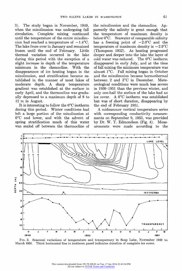
3). The study began in November, 1949, when the mixolimnion was undergoing fall circulation. Complete mixing continued until the temperature of the entire mixolimnion had reached a temperature of -1.40C. The lake froze over in January and remained frozen until the end of February. Little thermal variation occurred in the lake during this period with the exception of a slight increase in depth of the temperature minimum in the chemocline. With the disappearance of ice heating began in the mixolimnion, and stratification became established in the manner of most lakes of moderate depth. A sharp temperature gradient was established at the surface in early April, and the thermocline was gradually depressed to a maximum depth of 8 to 12 m in August.

It is interesting to follow the 0?C isotherm during this period. Winter conditions had left a large portion of the mixolimnion at 0?C and lower, and with the advent of spring stratification much of this water was sealed off between the thermocline of

the mixolimnion and the chemocline. Ap- parently the salinity is great enough that the temperature of maximum density is below 0?C. Seawater of comparable salinity has a freezing point of -2.0?C and the temperature of maximum density is -2.9?C (Thompson 1932). As heating progressed deeper and deeper into the lake the layer of cold water was reduced. The 0?C isotherm disappeared in early July, and at the time of fall mixing the minimum temperature was almost 1VC. Fall mixing began in October and the mixolimnion became hormothermal between 2 and 3?C in December. Mete- orological conditions were much less severe in 1950-1951 than the previous winter, and only one-half the surface of the lake had an ice cover. A 0?C isotherm was established but was of short duration, disappearing by the end of February 1951.

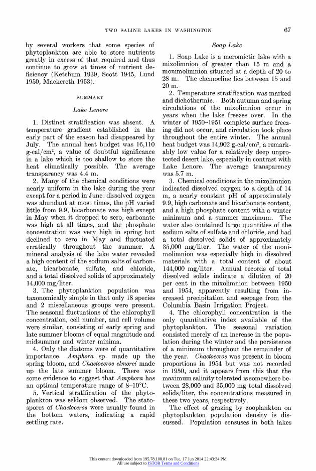
A midsummer vertical temperature series with corresponding conductivity measurements on September 9, 1953, was provided by Dr. W. T. Edmondson (Fig. 4). Meas- urements were made according to the

0 LAKE LEVEL

4

D J F M A M J J A S 0 N D J F M 1949 1950 195 1

FIG. 3. Seasonal variations of temperature and transparency in Soap Lake, November 1949 to 1\'larch 1951. Thick horizontal line in isotherm panel indicates duration of complete ice cover.



62 G. C. ANDERSON

0 c .

0 5 10 15 20 25

5

CONDUCTIVITY TEMPERATURE

10

i '5

I-

w

20

265

20 30 40 50 60 70

THOUSANDS OF MICROMHOS

FIG. 4. Vertical variations of temperature and conductivity in Soap Lake, September 9, 1953.

method outlined by Edmondson (1956). Conductivity and temperature were nearly uniform from the surface to a depth of 14 m, the extent of the epilimnion. At 20 m the temperature dropped to 3.4?C, but below this depth gradually increased to 5.40C at the bottom. The conductivity showed a gradual but small increase from 14 to 20 m, and beyond this depth a more than two-fold increase in conductivity was observed. There was a major difference in the extent of heating in the lake in 1950 and 1953. In September, 1950, the bottom of the epilimnion was at a depth of 8 m and the temperature minimum of the chemocline was 0.6?C, whereas in 1953 a layer of uniform salinity and temperature extended to a depth of 14 m and the temperature minimum of the chemocline was 3.4?C.

The annual heat budget calculated for Soap Lake was 14,902 g-cal/cm2 of lake surface. The value is small, especially when one considers the fact that Soap Lake is located in a hot dry desert climate. Also, the lake is completely exposed to winds from a north-south direction and has some degree of, but by no means complete, pro-

tection from winds from an east or west direction. This illustrates the remarkable stability of Soap Lake which is of course necessary to maintain meromixis and which has been commented on for other meromictic lakes (Hutchinson 1937).

Transparency. The transparency ranged from a minimum of 1 m on January 28, 1950, to a maximum of 11 m on July 29, 1950 (Fig. 3). There was a sustained winter minimum. Transparency was high during most of the summer and decreased in the latter part of September and October. The arithmetic average for the period studied was 5.7 m.

Total solids. Some records of the total solids concentration in Soap Lake since 1945 are available. U. S. Bureau of Recla- mation data show that the approximate average of total solids in the mixolimnion from 1945 through 1950 was 35,000 mg/ liter. In 1949 the lake level began to rise, and it was suspected that the lake was being "freshened" by increased precipitation and underground seepage from the surrounding irrigation project. On May 16, 1954, a vertical series of total solids revealed that the average concentration in the mixolimnion was 28,000 mg/liter, which indicated a dilution of 20 per cent. No significant change was detected in the monimolimnion, the maximum recorded being 144,000 mg/ liter.

Dissolved oxygen. Little interpretation can be made of the oxygen data owing to the uncertainty of the technique and to the short period of measurements, May 20 to November 4, 1950. Oxygen in the surface waters was generally low, never exceeding 6.6 mg/liter. There was an increase in oxygen concentration in waters of the 10 m depth zone in midsummer which was probably due to photosynthesis below the thermocline. There was no oxygen present at any time below 15 m, and on only two occasions was there even a slight trace of oxygen at 15 m.

Hydrogen-ion concentration. The range of pH was small, which demonstrates the highly buffered nature of the water. A maximum of pH 10.0 occurred in the




mixolimnion on April 22, 1950, and a minimum of 9.4 was recorded in the monimolimnion on August 12, 1950.

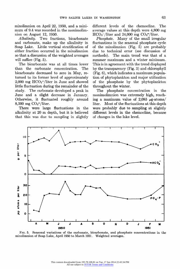
Alkalinity. Two fractions, bicarbonate and carbonate, make up the alkalinity in Soap Lake. Little vertical stratification of either fraction occurred in the mixolimnion so that a discussion of the weighted averages will suffice (Fig. 5).

The bicarbonate was at all times lower than the carbonate concentration. The bicarbonate decreased to zero in May, returned to its former level of approximately 2,000 mg HCO3-/liter in June and showed little fluctuation during the remainder of the study. The carbonate developed a peak in June and a slight decrease in January. Otherwise, it fluctuated roughly around 8,500 mg C03-/liter.

There were large fluctuations in the alkalinity at 20 m depth, but it is believed that this was due to sampling in slightly

different levels of the chemocline. The average values at this depth were 4,800 mg HCO3-/liter and 24,000 mg C03-/liter.

Phosphate. Many of the small irregular fluctuations in the seasonal phosphate cycle of the mixolimnion (Fig. 5) are probably due to technical error (see discussion of methods). The main trend was that of a summer maximum and a winter minimum. This is in agreement with the trend displayed by the transparency (Fig. 3) and chlorophyll (Fig. 6), which indicates a maximum population of phytoplankton and major utilization of the phosphate by the phytoplankton throughout the winter.

The phosphate concentration in the monimolimnion was extremely high, reach- ing a maximum value of 2,085 ,ug-atoms/ liter. Most of the fluctuations at this depth were probably due to sampling at slightly different levels in the chemocline, because of changes in the lake level.

10

C 03

0 ~ ~ ~ ~ ~ ~ ~ ~ ~ ~~~~~~~~~~~~~~~HC0 305

20 -

E 10 _

4 I4

c 0

I I I I _ I I I I I A M J J A S 0 N D J F M

1950 19SI FIG. 5. Seasonal variations of the carbonate, bicarbonate, and phosphate concentrations in the

mixolimnion of Soap Lake, April 1950 to March 1951. Weighted averages.



64 G. C. ANDERSON

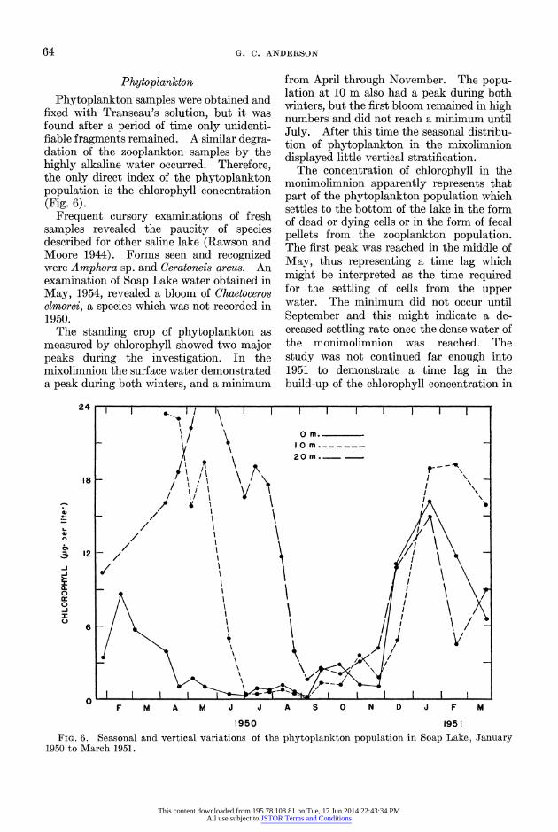
Phytoplankton Phytoplankton samples were obtained and

fixed with Transeau's solution, but it was found after a period of time only unidenti- fiable fragments remained. A similar degra- dation of the zooplankton samples by the highly alkaline water occurred. Therefore, the only direct index of the phytoplankton population is the chlorophyll concentration (Fig. 6).

Frequent cursory examinations of fresh samples revealed the paucity of species described for other saline lake (Rawson and Moore 1944). Forms seen and recognized were Amphora sp. and Ceratoneis arcus. An examination of Soap Lake water obtained in May, 1954, revealed a bloom of Chaetoceros elmorei, a species which was not recorded in 1950.

The standing crop of phytoplankton as measured by chlorophyll showed two major peaks during the investigation. In the mixolimnion the surface water demonstrated a peak during both winters, and a minimum

from April through November. The population at 10 m also had a peak during both winters, but the first bloom remained in high numbers and did not reach a minimum until July. After this time the seasonal distribution of phytoplankton in the mixolimnion displayed little vertical stratification.

The concentration of chlorophyll in the monimolimnion apparently represents that part of the phytoplankton population which settles to the bottom of the lake in the form of dead or dying cells or in the form of fecal pellets from the zooplankton population. The first peak was reached in the middle of May, thus representing a time lag which might be interpreted as the time required for the settling of cells from the upper water. The minimum did not occur until September and this might indicate a decreased settling rate once the dense water of the monimolimnion was reached. The study was not continued far enough into 1951 to demonstrate a time lag in the build-up of the chlorophyll concentration in

24i I , \ I O m _ I

20 M

18 ~ ~ 1

0

FIG. 6. Seasonal and vertical variations of the phytoplankton population in Soap Lake, Janulary 1950 to March 1951.




the monimolimnion after the 1951 winter peak of phytoplankton in the mixolimnion.

The presence of Chaetoceros elmorei in 1954 and its apparent absence in 1950 pro- vides additional information on the salinity tolerance of the species. Rawson and Moore (1944) reported Chaetoceros in lakes having total solids concentration of up to 30,000 mg/liter. The next lake in their series had a concentration of 120,000 mg/ liter, and Chaetoceros was not present. From these data it could be ascertained only that the critical level lay somewhere between these two values. Soap Lake affords the opportunity to come much closer to an estimate of the critical level. In 1950 the total solids averaged 35,000 mg/liter and in 1954, 28,000 mg/liter. Chaetoceros was at bloom level of abundance in May, 1954 so that the critical value probably is in excess of 28,000 mg/liter, but of course less than 35,000 mg/liter.

EFFECT OF GRAZING

It has been reported previously that a high production rate of phytoplankton in Soap Lake may have been masked during the spring and summer season due to a large population of grazers (Anderson et al. 1955). The zooplankters, Moina hutchinsoni Brehm, Hexarthra (= Pedalia) fennica (Levander), and Brachionus plicatilis Muller, were in great abundance during the summer period of phytoplankton minimum, and a clear reciprocal relationship was found with the phytoplankton. In Lake Lenore the first spring phytoplankton maximum was followed by a pulse of Moina and Diaptomus sicilis Forbes, and the late-summer phytoplankton peak was followed by a resurgence of Moina, Diaptomus, and Hexarthra. Thus, it was concluded that the most probable interpretation of the seasonal changes observed in size of the phytoplankton population is its control by the grazing activity of the zooplankton.

In order to demonstrate further the effect of grazing on phytoplankton population density, two attempts were made to measure directly the amount of grazing in July and October, 1955. Two one-gallon jugs of lake water were suspended in both Soap

Lake and Lake Lenore. One jug contained the raw lake water and the other contained lake water which had been filtered with number-10 mesh silk net to remove only the zooplankton. In the July experiment zooplankton was added to the unfiltered jug to increase the population approximately twofold, whereas in the October experiment, conditions were not modified in the unfiltered jug. The initial population density was measured by means of chlorophyll concentration, and the jugs were left for a period of a few days. Differences in chlorophyll concentration between filtered and unfiltered jugs indicated the amount of grazing.

In both experiments in Soap Lake, there was evidence that grazing significantly reduced the phytoplankton population size, since a much higher chlorophyll concentration developed in the jug from which zooplankton had been removed. The data are not conclusive for Lake Lenore since both the filtered and unfiltered water contained approximately equal concentrations of chlorophyll at the end of the experiment (Table 5). At present there is no explana- tion for the apparent failure of the zooplankton to decrease the phytoplankton concentration in the Lake Lenore population. The net increase in chlorophyll of all jugs over the initial concentration can probably be attributed to the added growth of periphytic algae on the glass walls. The data would have more significance had cell counts been made in addition to the chlorophyll measurements but this was not pos-

TABLE 5. The effect of grazing by zooplankton on phytoplankton population density as shown by gallon jugs containing filtered and unfiltered Soap Lake and Lake Lenore water suspended in each lake for certain intervals of time in 1955

Soap Lake Lake Lenore

July 3- Oct. 19- July 2- Oct. 19- July 7 Oct. 25 July 6 Oct. 25 102 hr 145 hr 99 hr 144 hr

Chlorophyll (,g/liter) Initial 0.45 3.15 0.30 2.40 Final

Zooplankton present 0 75 5.10 0.60 3.60 Zooplankton absent 1.80 5.55 0.60 3.45

Zooplankton (no./liter) Copepoda 472 105 Cladocera 185 12 90 34 Rotifera 70 154 614 93



66 G. C. ANDERSON

sible due to preservation difficulties. Only recently it has been demonstrated that the chlorophyll content of phytoplankton populations may show marked diurnal variations independent of changes in population size due to cell division or death (Yentsch and Ryther 1957).

DISCUSSION

Although Soap Lake and Lake Lenore are similar in origin and are situated in close proximity, the two lakes are quite different in structure and metabolism owing chiefly to the greater depth and salt content of Soap Lake. Soap Lake has permanent stratification, while stratification is virtu- ally absent in Lake Lenore. As a result, Soap Lake has a large store of nutrients in the monimolimnion, a small fraction of which might be mixed with the surface waters during the overturn of the mixolimnion, whereas the transport of nutrients from the bottom waters in Lake Lenore is continuous.

One of the striking similarities found between the two lakes was the lack of variety of phytoplankton organisms, which is evidently a characteristic of highly saline lakes. Although a qualitative list of organisms for Soap Lake was not determined, due to preservation difficulties, frequent examination of fresh samples revealed the paucity of species. A total of only 18 species was found in Lake Lenore. Rawson and Moore (1944) recorded a total of 13 species of algae from Little Manitou Lake, a saline lake in Saskatchewan. Although the lake has a salinity approximately eight times as great as Lenore and is also qualitatively different, it demonstrates the paucity of species occurring in highly saline lakes. In six other lakes in Saskatchewan, of the same magnitude of salinity as Lenore, there was a total of 34 species of algae that were occasional to abundant. Hutchinson (1937) found the same paucity of species in his study of saline lakes in the Lahontan Basin of Nevada. It should be pointed out that the Washington lakes are different from those in Saskatchewan in that the more saline lakes of Saskatchewan are of the sulfate type with usually more magnesium

than sodium and are not especially alkaline, having a pH range from 8.0 to 8.9 with the exception of Manitou Lake, which had a pH of 9.5.

The seasonal fluctuations of the total standing crop of phytoplankton were quite different in the two lakes. Lake Lenore followed the pattern found in many described freshwater lakes in that two well- defined major peaks of population density occurred, an early spring and a late summer peak. Soap Lake was unusual in that the one annual peak observed occurred during the winter beneath the ice cover in 1950 and during the coldest part of the year in January, 1951. However, from experimental evidence in Soap Lake and from the sequence of phytoplankton-zooplankton events in both lakes, it appears that the most probable interpretation of the seasonal fluctuations observed is that of control of phytoplankton population size by the grazing activity of the zooplankton.

Since phytoplankton organisms must absorb nutrients for growth, it may be expected that a high concentration of nutrients will ordinarily not be maintained in the presence of a large phytoplankton population, and large increases in the population will usually be accompanied by a decrease in the nutrient concentration. See, for example, the sudden drop in phosphate concentration in Lake Lenore after the occurrence of the two maj or blooms of phytoplankton (Figs. 1 and 2), and the build-up of phosphate in Soap Lake during phytoplankton minima in midsummer 1950 and early spring 1951 (Figs. 5 and 6). However, the relationship is not always clear. The fact that nutrients are often rapidly released by action of bacteria and other heterotrophic organisms may obscure the relation, and at many times the concentration of nutrients may be a minor factor in governing the size of the phytoplankton population, other factors such as grazing, parasitism, light, temperature, etc., or combinations of the above being the limiting factors. It is possible, at times, that the nutrient supply is in excess and its rate of supply greater than the demand being made upon it by the phytoplankton, and also it has been shown




by several workers that some species of phytoplankton are able to store nutrients greatly in excess of that required and thus continue to grow at times of nutrient de- ficiency (Ketchum 1939, Scott 1945, Lund 1950, Mackereth 1953).

SUMMARY

Lake Lenore

1. Distinct stratification was absent. A temperature gradient established in the early part of the season had disappeared by July. The annual heat budget was 16,110 g-cal/cm2, a value of doubtful significance in a lake which is too shallow to store the heat climatically possible. The average transparency was 4.4 m.

2. Many of the chemical conditions were nearly uniform in the lake during the year except for a period in June: dissolved oxygen was abundant at most times, the pH varied little from 9.9, bicarbonate was high except in May when it dropped to zero, carbonate was high at all times, and the phosphate concentration was very high in spring but declined to zero in May and fluctuated erratically throughout the summer. A mineral analysis of the lake water revealed a high content of the sodium salts of carbonate, bicarbonate, sulfate, and chloride, and a total dissolved solids of approximately 14,000 mg/liter.

3. The phytoplankton population was taxonomically simple in that only 18 species and 2 miscellaneous groups were present. The seasonal fluctuations of the chlorophyll concentration, cell number, and cell volume were similar, consisting of early spring and late summer blooms of equal magnitude and midsummer and winter minima.

4. Only the diatoms were of quantitative importance. Amphora sp. made up the spring bloom, and Chaetoceros elmorei made up the late summer bloom. There was some evidence to suggest that Amphora has an optimal temperature range of 8-100C.

5. Vertical stratification of the phytoplankton was seldom observed. The statospores of Chaetoceros were usually found in the bottom waters, indicating a rapid settling rate.

Soap Lake

1. Soap Lake is a meromictic lake with a mixolimnion of greater than 15 m and a monimolimnion situated at a depth of 20 to 28 m. The chemocline lies between 15 and 20 m.

2. Temperature stratification was marked and dichothermic. Both autumn and spring circulations of the mixolimnion occur in years when the lake freezes over. In the winter of 1950-1951 complete surface freezing did not occur, and circulation took place throughout the entire winter, The annual heat budget was 14,902 g-cal/cm2, a remark- ably low value for a relatively deep unpro- tected desert lake, especially in contrast with Lake Lenore. The average transparency was 5.7 m.

3. Chemical conditions in the mixolimnion indicated dissolved oxygen to a depth of 14 m, a nearly constant pH of approximately 9.9, high carbonate and bicarbonate content, and a high phosphate content with a winter minimum and a summer maximum. The water also contained large quantities of the sodium salts of sulfate and chloride, and had a total dissolved solids of approximately 35,000 mg/liter. The water of the monimolimnion was especially high in dissolved materials with a total content of about 144,000 mg/liter. Annual records of total dissolved solids indicate a dilution of 20 per cent in the mixolimnion between 1950 and 1954, apparently resulting from increased precipitation and seepage from the Columbia Basin Irrigation Project.

4. The chlorophyll concentration is the only quantitative index available of the phytoplankton. The seasonal variation consisted merely of an increase in the population during the winter and the persistence of a minimum throughout the remainder of the year. Chaetoceros was present in bloom proportions in 1954 but was not recorded in 1950, and it appears from this that the maximum salinity tolerated is somewhere between 28,000 and 35,000 mg total dissolved solids/liter, the concentrations measured in these two years, respectively.

The effect of grazing by zooplankton on phytoplankton population density is discussed. Population censuses in both lakes



68 G. C. ANDERSON

and experimental evidence for Soap Lake suggest that interpretation of the seasonal fluctuations of phytoplankton involves a control by grazing.

REFERENCES

AMERICAN PUBLIC HEALTH ASSOCIATION. 1946. Standard methods for the examination of water and sewage. 9th ed. New York. 286 PP.

ANDERSON, G. C., G. W. COMITA, AND VERNA ENGSTROM-HEG. 1955. A note on the phytoplankton-zooplankton relationships in two lakes in Washington. Ecology, 36: 757-759.

BEADLE, L. C. 1943. An ecological survey of some inland saline waters of Algeria. J. Linn. Soc. Zool., 41: 218-242.

BRETZ, J. H. 1932. The Grand Coulee. Amer. Geog. Soc., Spec. Publ. No. 15. 89 pp.

EDMONDSON, W. T. 1956. Measurements of conductivity of lake water in situ. Ecology, 37: 201-204.

EDMONDSON, W. T., AND Y. H. EDMONDSON. 1947. Measurements of production in fer- tilized salt water. J. Mar. Res., 6: 228-246.

EINSELE, W. 1941. Die Umsetzung von zuge- filhrtem, anorganischen Phosphat im euitro- phen Seen und ihre Ruickwirkungen auf seinen Gesamthaushalt. Z. Fisch., 39: 407- 488.

HUTCHINSON, G. E. 1937. A contribution to the limnology of arid regions. Trans. Conn. Acad. Arts Sci., 33: 47-132.

KETCHUM, B. H. 1939. The development and restoration of deficiencies in the phosphorus and nitrogen composition of unicellular plants. J. Cell. Comp. Physiol., 13: 373-381.

LACKEY, J. B. 1938. The manipulation and counting of river plankton and changes in some organisms due to formalin preservation. U. S. Pub. Health Rep., 53: 2080-2093.

LUND, J. W. G. 1950. Studies on Asterionella formosa Hass. II. Nutrient depletion and the spring maximum. Part I. Observations on Windermere, Esthwaite Water and Blel- ham Tarn. Part II. Discussion. J. Ecol., 38: 1-35.

MACKERETH, F. J. 1953. Phosphorus utilization by Asterionella formosa Hass. J. Exp. Bot., 4: 296-313.

MUNDORFF, M. J., AND G. L. BODHAINE. 1954. Investigation of the rise in level of Soap Lake at Soap Lake, Washington. Open-file report of the Water Resources Division, U. S. Geological Survey, Tacoma District, 117 pp.

RAWSON, D. S., AND J. E. MOORE. 1944. The saline lakes of Saskatchewan. Can. J. Res., 22: 141-201.

ROBINSON, R. J., AND T. G. THOMPSON. 1948. The determination of phosphates in sea water. J. Mar. Res., 7: 33-41.

SCHEFFER, T. H. 1946. Aquatic plants of the Grand Coulee, Washington. Arboretum Bull., Arboretum Foundation, Seattle, Wash- ington. 4 pp.

SCOTT, G. T. 1945. The mineral composition of phosphate deficient cells of Chorella pyre- noidosa during the restoration of phosphate. J. Cell. Comp. Physiol., 26: 35-42.

THOMPSON, T. G. 1932. The physical properties of sea water. Bull. Nat. Res. Council, No. 85, pp. 63-94.

YENTSCH, C. S., AND J. H. RYTHER. 1957. Short-term variations in phytoplankton chlorophyll and their significance. Limnol. & Oceanogr., 2: 140-142.

YOUNG, R. T. 1924. The life of Devils Lake, North Dakota. Pub. North Dakota Biol. Station, 116 pp.

ZWICKER, B. M. G., AND R. J. ROBINSON. 1944. The photometric determination of nitrate in sea water with a strychnidine reagent. J. Mar. Res., 4: 214-232.



seasonal characteristics of two saline lakes in washington

Documents