seari short course series

seari.mit.edu

SEAri Short Course Series Course: PI.27s Value-driven Tradespace Exploration for System Design Lecture: Lecture 5: Modeling and Exploring the Tradespace Author: Adam Ross and Donna Rhodes Lecture Number: SC-2009-1-5-1 Revision Date: August 11, 2009 A slightly earlier version of this course was taught at PI.27s as a part of the MIT Professional Education Short Programs in June 2009 in Cambridge, MA. The lectures are provided to satisfy demand for learning more about Multi-Attribute Tradespace Exploration, Epoch-Era Analysis, and related SEAri-generated methods. The course is intended for self-study only. The materials are provided without instructor support, exercises or “course notebook” contents. Do not separate this cover sheet from the accompanying lecture pages. The copyright of the short course is retained by the Massachusetts Institute of Technology. Reproduction, reuse, and distribution of the course materials are not permitted without permission.

PI.27s VALUE-DRIVEN TRADESPACE EXPLORATIONFOR SYSTEM DESIGN

Lecture 5Modeling and Exploring the Tradespace

Dr. Donna Rhodes and Dr. Adam M. RossMIT

seari.mit.edu © 2009 Massachusetts Institute of Technology 2

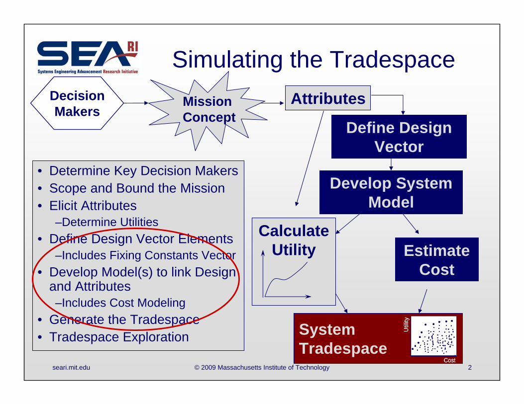
Simulating the Tradespace

• Determine Key Decision Makers• Scope and Bound the Mission• Elicit Attributes

–Determine Utilities• Define Design Vector Elements

–Includes Fixing Constants Vector• Develop Model(s) to link Design

and Attributes–Includes Cost Modeling

• Generate the Tradespace• Tradespace Exploration

MissionConcept

Attributes

Calculate Utility

Develop System Model

Estimate Cost

SystemTradespace

Define Design Vector

Decision Makers

Cost

Util

ity

Cost

Util

ity


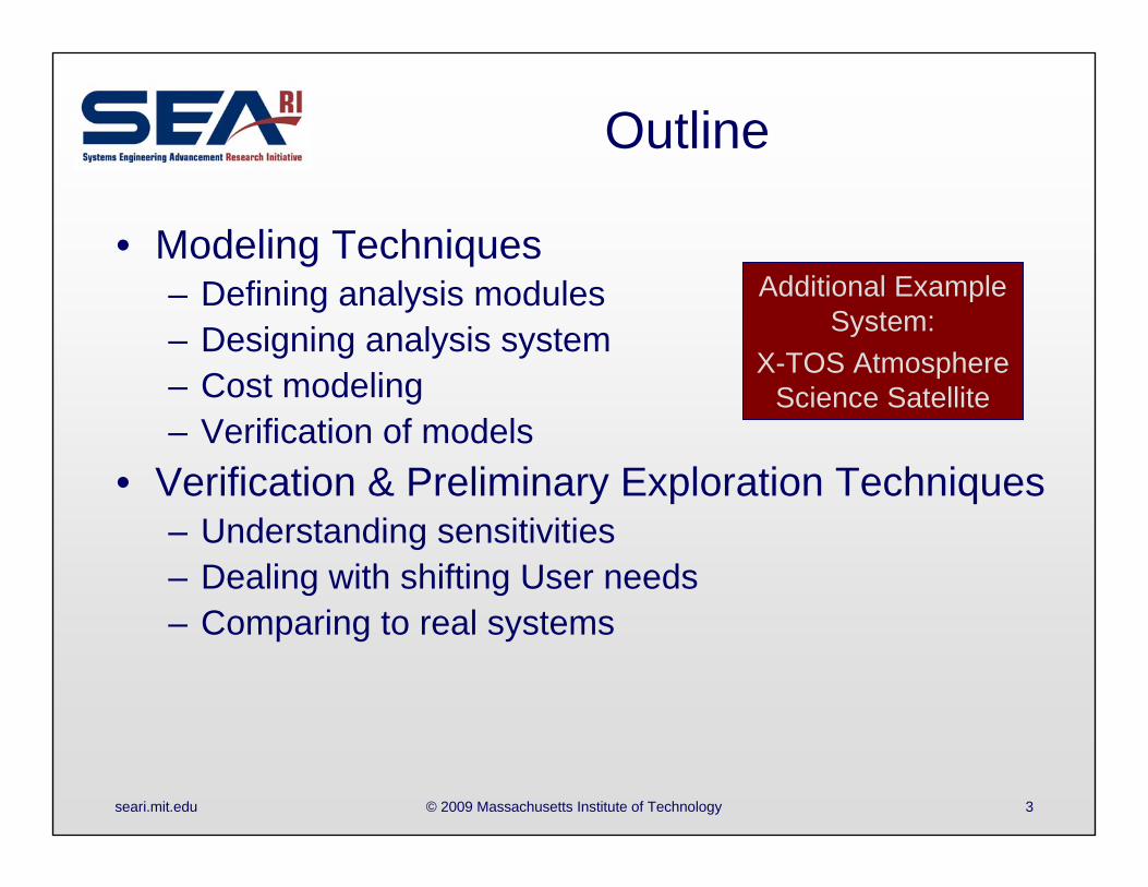
Outline

• Modeling Techniques– Defining analysis modules– Designing analysis system– Cost modeling– Verification of models

• Verification & Preliminary Exploration Techniques– Understanding sensitivities– Dealing with shifting User needs– Comparing to real systems

Additional Example System:

X-TOS Atmosphere Science Satellite


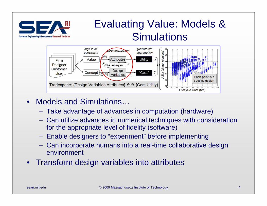
Evaluating Value: Models & Simulations

• Models and Simulations…– Take advantage of advances in computation (hardware)– Can utilize advances in numerical techniques with consideration

for the appropriate level of fidelity (software)– Enable designers to “experiment” before implementing– Can incorporate humans into a real-time collaborative design

environment• Transform design variables into attributes


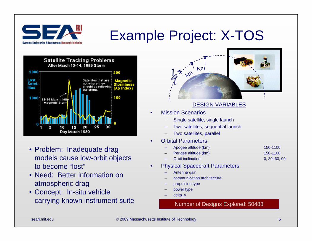
Example Project: X-TOS

Number of Designs Explored: 50488

DESIGN VARIABLES• Mission Scenarios

– Single satellite, single launch– Two satellites, sequential launch– Two satellites, parallel

• Orbital Parameters– Apogee altitude (km) 150-1100– Perigee altitude (km) 150-1100– Orbit inclination 0, 30, 60, 90

• Physical Spacecraft Parameters– Antenna gain– communication architecture– propulsion type– power type– delta_v

kmKm

• Problem: Inadequate drag models cause low-orbit objects to become “lost”

• Need: Better information on atmospheric drag

• Concept: In-situ vehicle carrying known instrument suite


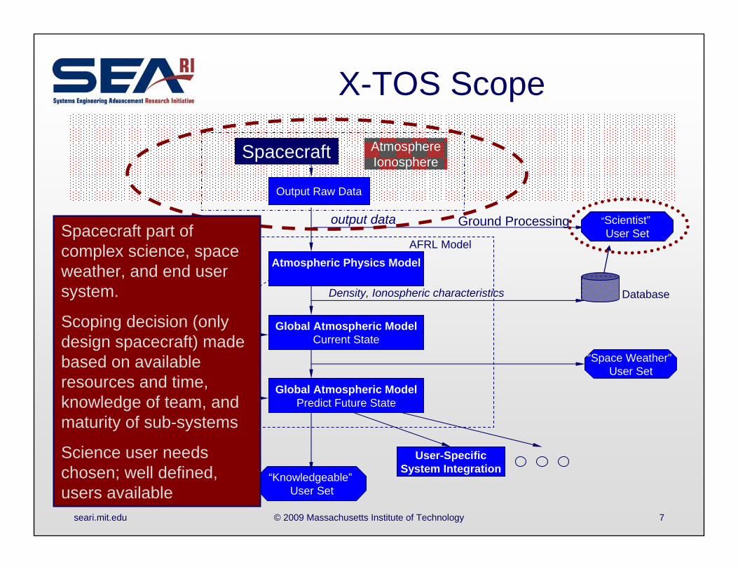
X-TOS ScopeAtmosphereIonosphereSpacecraft

Atmospheric Physics Model

Global Atmospheric ModelCurrent State

Global Atmospheric ModelPredict Future State

User-SpecificSystem Integration

AFRL Model

output data “Scientist”User Set

“Space Weather”User Set

“Knowledgeable”User Set

Density, Ionospheric characteristics Database

Other Data Sources

(Various assets)

Ground Processing

Output Raw Data


X-TOS ScopeAtmosphereIonosphereSpacecraft

Atmospheric Physics Model

Global Atmospheric ModelCurrent State

Global Atmospheric ModelPredict Future State

User-SpecificSystem Integration

AFRL Model

output data “Scientist”User Set

“Space Weather”User Set

“Knowledgeable”User Set

Density, Ionospheric characteristics Database

Other Data Sources

(Various assets)

Ground Processing

Output Raw Data

Spacecraft part of complex science, space weather, and end user system.

Scoping decision (only design spacecraft) made based on available resources and time, knowledge of team, and maturity of sub-systems

Science user needs chosen; well defined, users available


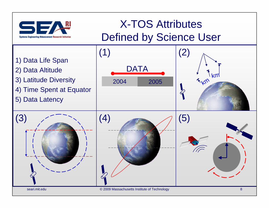
X-TOS AttributesDefined by Science User

(5)(4)(3)

(2)(1)1) Data Life Span2) Data Altitude3) Latitude Diversity4) Time Spent at Equator5) Data Latency

kmkm

2004 2005

DATA


Generating DV-Att Mappings

QFD X-TOS

CO

NST

RA

INTS

DESIGN-ATTRIBUTE

Uni

ts

% $ (2

002)

ATT

RIB

UTE

S

Dis

tribu

tion

of A

ltitu

des

Num

ber o

f Alti

tude

Ban

ds

Dis

tribu

tion

of L

atitu

des

Num

ber o

f Lat

itude

s

Dis

tribu

tion

of T

ime/

Cyc

les

Tota

l Dat

a P

oint

s

Sam

ple

Res

olut

ion

Sam

ple

Accu

racy

Dat

a C

ompl

eten

ess/

Mis

sion

Suc

ces

TOTA

L (U

SER

)

Life

cycl

e C

ost

Tota

l (C

UST

OM

ER)

Ease

of M

odel

ing

Tota

l (D

ESIG

NER

)

1 2 3 4 5 6 7 8 9 10 11

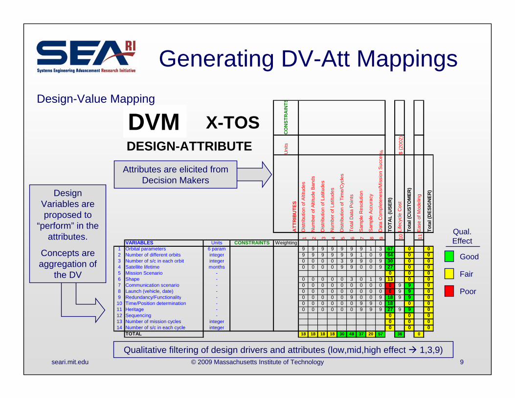
VARIABLES Units CONSTRAINTS Weighting1 Orbital parameters 6 param 9 9 9 9 9 9 9 1 3 67 0 02 Number of different orbits integer 9 9 9 9 9 9 1 0 9 64 0 03 Number of s/c in each orbit integer 0 0 0 0 3 9 9 0 9 30 0 04 Satellite lifetime months 0 0 0 0 9 9 0 0 9 27 0 05 Mission Scenario - 0 0 06 Shape - 0 0 0 0 0 3 0 1 9 13 0 07 Communication scenario - 0 0 0 0 0 0 0 0 0 0 9 9 08 Launch (vehicle, date) - 0 0 0 0 0 0 0 0 0 0 9 9 09 Redundancy/Functionality - 0 0 0 0 0 9 0 0 9 18 9 9 0

10 Time/Position determination - 0 0 0 0 0 0 9 9 0 18 0 011 Heritage - 0 0 0 0 0 0 9 9 9 27 9 9 012 Sequencing - 0 0 013 Number of mission cycles integer 0 0 014 Number of s/c in each cycle integer 0 0 0

TOTAL 18 18 18 18 30 48 37 20 57 36 0

Design Variables are proposed to

“perform” in the attributes.

Concepts are aggregation of

the DV

Attributes are elicited from Decision Makers

Qualitative filtering of design drivers and attributes (low,mid,high effect 1,3,9)

Qual. Effect

Poor

Good

Fair

DVMDesign-Value Mapping


Generating DV-Att Mappings

QFD X-TOS

CO

NST

RA

INTS

DESIGN-ATTRIBUTE

Uni

ts

% $ (2

002)

ATT

RIB

UTE

S

Dis

tribu

tion

of A

ltitu

des

Num

ber o

f Alti

tude

Ban

ds

Dis

tribu

tion

of L

atitu

des

Num

ber o

f Lat

itude

s

Dis

tribu

tion

of T

ime/

Cyc

les

Tota

l Dat

a P

oint

s

Sam

ple

Res

olut

ion

Sam

ple

Accu

racy

Dat

a C

ompl

eten

ess/

Mis

sion

Suc

ces

TOTA

L (U

SER

)

Life

cycl

e C

ost

Tota

l (C

UST

OM

ER)

Ease

of M

odel

ing

Tota

l (D

ESIG

NER

)

1 2 3 4 5 6 7 8 9 10 11

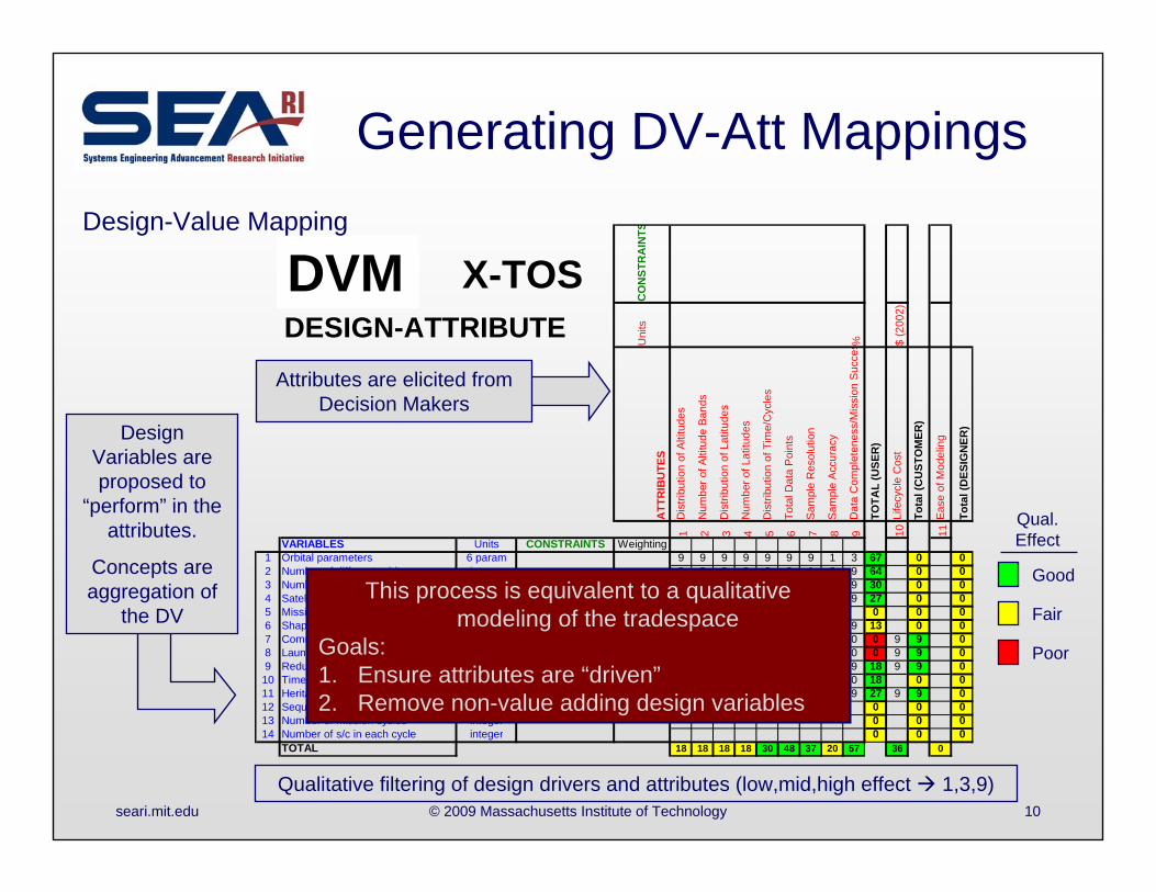
VARIABLES Units CONSTRAINTS Weighting1 Orbital parameters 6 param 9 9 9 9 9 9 9 1 3 67 0 02 Number of different orbits integer 9 9 9 9 9 9 1 0 9 64 0 03 Number of s/c in each orbit integer 0 0 0 0 3 9 9 0 9 30 0 04 Satellite lifetime months 0 0 0 0 9 9 0 0 9 27 0 05 Mission Scenario - 0 0 06 Shape - 0 0 0 0 0 3 0 1 9 13 0 07 Communication scenario - 0 0 0 0 0 0 0 0 0 0 9 9 08 Launch (vehicle, date) - 0 0 0 0 0 0 0 0 0 0 9 9 09 Redundancy/Functionality - 0 0 0 0 0 9 0 0 9 18 9 9 0

10 Time/Position determination - 0 0 0 0 0 0 9 9 0 18 0 011 Heritage - 0 0 0 0 0 0 9 9 9 27 9 9 012 Sequencing - 0 0 013 Number of mission cycles integer 0 0 014 Number of s/c in each cycle integer 0 0 0

TOTAL 18 18 18 18 30 48 37 20 57 36 0

Design Variables are proposed to

“perform” in the attributes.

Concepts are aggregation of

the DV

Attributes are elicited from Decision Makers

Qualitative filtering of design drivers and attributes (low,mid,high effect 1,3,9)

Qual. Effect

Poor

Good

FairThis process is equivalent to a qualitative

modeling of the tradespaceGoals: 1. Ensure attributes are “driven”2. Remove non-value adding design variables

DVMDesign-Value Mapping


Determining the Design VectorQFD X-TOS

CO

NST

RA

INTS

DESIGN-ATTRIBUTE

Uni

ts

degr

ees

year

s

% km min

utes

inte

ger

% $ (2

002)

$/yr

? time

? ?

ATT

RIB

UTE

S

Atm

osph

eric

Cov

erag

e

Life

time

% o

rbit

in d

ata

regi

on

Kno

wle

dge

accu

racy

of a

ltitu

de

Late

ncy

Num

ber o

f sim

ulta

neou

s da

ta p

oint

s

Qua

lity

of d

ata

/ dat

a co

mpl

eten

ess

TOTA

L (U

SER

)

Life

cycl

e C

ost

Res

ourc

e bu

rn

Mul

tiple

mis

sion

on

s/c

Sch

edul

e

Leav

e be

hind

cap

abili

ty

Ris

k

Tota

l (C

UST

OM

ER)

Eas

e of

Mod

elin

g

Tota

l (D

ESIG

NER

)

1 2 3 4 5 6 7 8 9 10 11 12 13 14

VARIABLES Units CONSTRAINTS Weighting1 Orbital parameters 6 param 9 9 9 9 9 9 9 63 1 3 4 02 Number of different orbits integer 9 9 9 9 9 9 1 55 0 9 9 03 Number of s/c in each orbit integer 0 0 0 0 3 9 9 21 0 9 9 04 Satellite lifetime months 0 0 0 0 9 9 0 18 0 9 9 05 Mission Scenario - 0 0 06 Shape - 0 0 0 0 0 3 0 3 1 9 10 07 Communication scenario - 0 0 0 0 9 0 0 9 0 0 9 9 08 Launch (vehicle, date) - 0 0 0 0 0 0 0 0 1 9 10 09 Redundancy/Functionality - 0 0 0 0 0 9 0 9 0 9 9 18 010 Time/Position determination - 0 0 0 0 0 0 9 9 9 0 9 011 Heritage - 0 0 0 0 0 0 9 9 9 9 9 27 012 Sequencing - 0 0 013 Number of mission cycles integer 0 0 014 Number of s/c in each cycle integer 0 0 0

TOTAL 18 18 18 18 39 48 37 0 0 0 21 57 36 0

QFD X-TOS

CO

NST

RA

INTS

0.5

- 11

150

- 100

0

0 - 1

80

0 - 2

4

1 - 1

20

0 -2

00

DESIGN-ATTRIBUTE

Uni

ts

Year

s

Km degr

ees

Hou

rs/d

a

Hou

rs

$M (2

002

ATT

RIB

UTE

S

Dat

a Li

fe S

pan

(Per

Sat

ellit

e)

Sam

ple

Altit

ude

Div

ersi

ty o

f Lat

itude

s co

ntai

ned

in

the

Dat

a Se

t

Tim

e Sp

ent i

n Eq

uato

rial R

egio

n

Late

ncy

TOTA

L (U

SER

)

Life

cycl

e C

ost

Func

tiona

lity

trade

abilit

y

Tota

l (C

UST

OM

ER)

Ease

of M

odel

ing

Tota

l (D

ESIG

NER

)

1 2 3 4 5 6 7 8

VARIABLES Units CONSTRAINTS Weighting1 Perigee Altitude m 150<hp<350 9 9 0 0 1 19 9 9 9 92 Apogee Altitude m 150<ha<1500 9 9 0 3 1 22 9 9 9 93 Inclination deg. 0<I<90 0 0 9 9 1 19 3 3 9 94 delta-V m/s 0<mass<500 9 0 0 0 0 9 9 9 3 35 Comm System Type - AFSCN or TDRSS 0 0 0 0 9 9 1 1 3 36 Antenna Gain - Low or High 0 0 0 0 9 9 3 3 3 37 Propulsion Type - Chemical or Hall 3 0 0 0 0 3 3 3 3 38 Power System Type - Solar or Fuel Cells 3 0 0 0 3 6 3 3 3 39 Mission Scenario - - 9 9 9 9 1 37 3 3 1 1

TOTAL 42 27 18 21 25 43 0 43

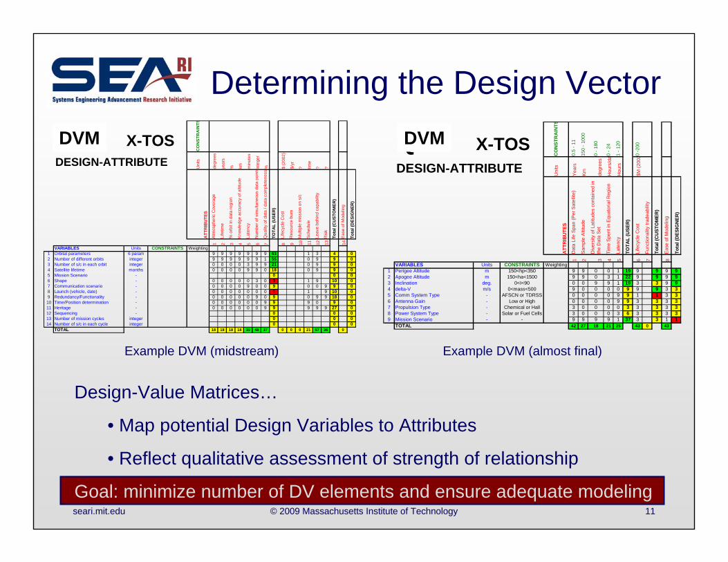
Example DVM (midstream) Example DVM (almost final)

Design-Value Matrices…

• Map potential Design Variables to Attributes

• Reflect qualitative assessment of strength of relationship

Goal: minimize number of DV elements and ensure adequate modeling

DVM DVM


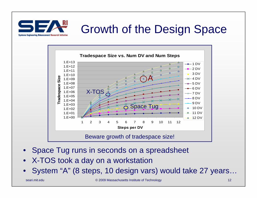
Growth of the Design Space

Tradespace Size vs. Num DV and Num Steps

1.E+001.E+011.E+021.E+031.E+041.E+051.E+061.E+071.E+081.E+091.E+101.E+111.E+121.E+13

1 2 3 4 5 6 7 8 9 10 11 12

Steps per DV

Trad

espa

ce S

ize

1 DV2 DV3 DV4 DV5 DV6 DV7 DV8 DV9 DV10 DV11 DV12 DV

Beware growth of tradespace size!

X-TOS

Space Tug

• Space Tug runs in seconds on a spreadsheet• X-TOS took a day on a workstation• System “A” (8 steps, 10 design vars) would take 27 years…

A


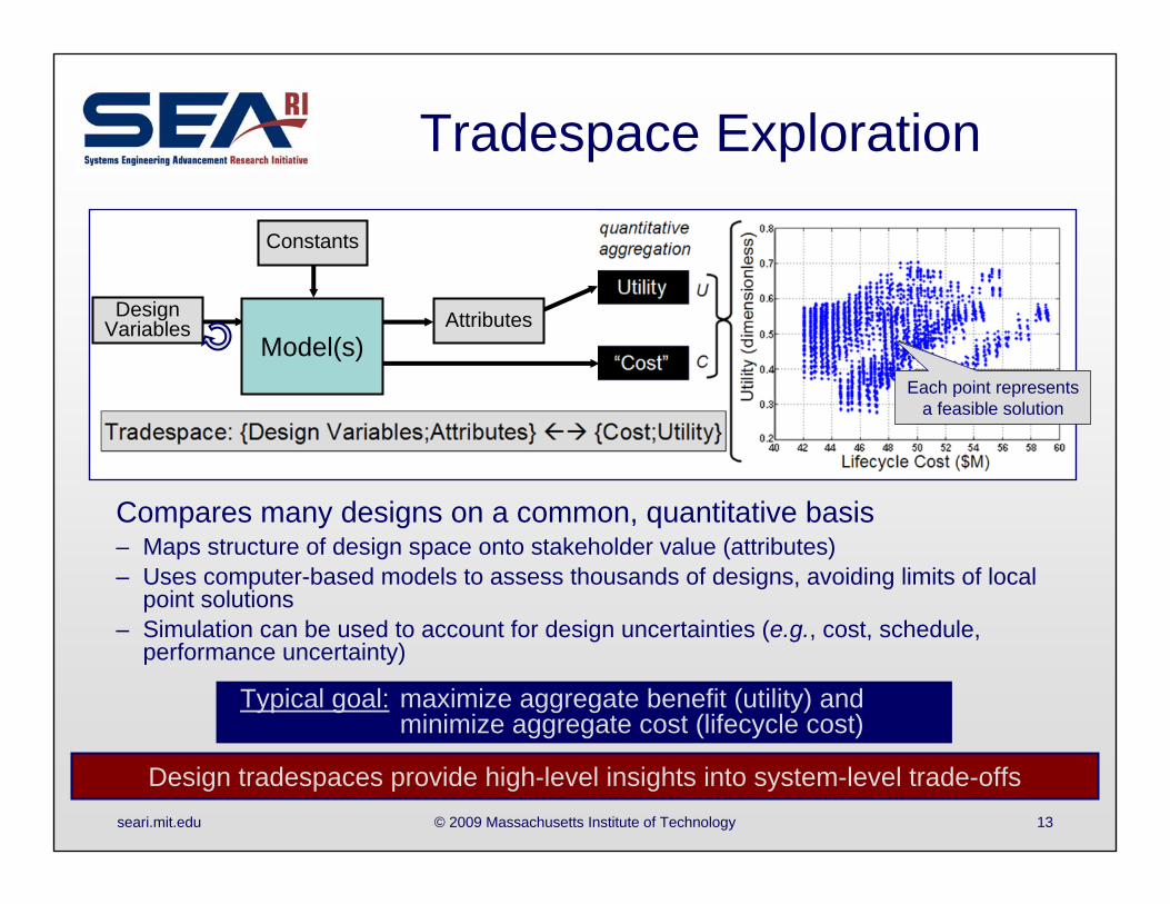
Tradespace Exploration

Compares many designs on a common, quantitative basis– Maps structure of design space onto stakeholder value (attributes)– Uses computer-based models to assess thousands of designs, avoiding limits of local

point solutions– Simulation can be used to account for design uncertainties (e.g., cost, schedule,

performance uncertainty)

Design tradespaces provide high-level insights into system-level trade-offs

Each point represents a feasible solution

Constants

Design Variables Attributes

Model(s)

Typical goal: maximize aggregate benefit (utility) andminimize aggregate cost (lifecycle cost)


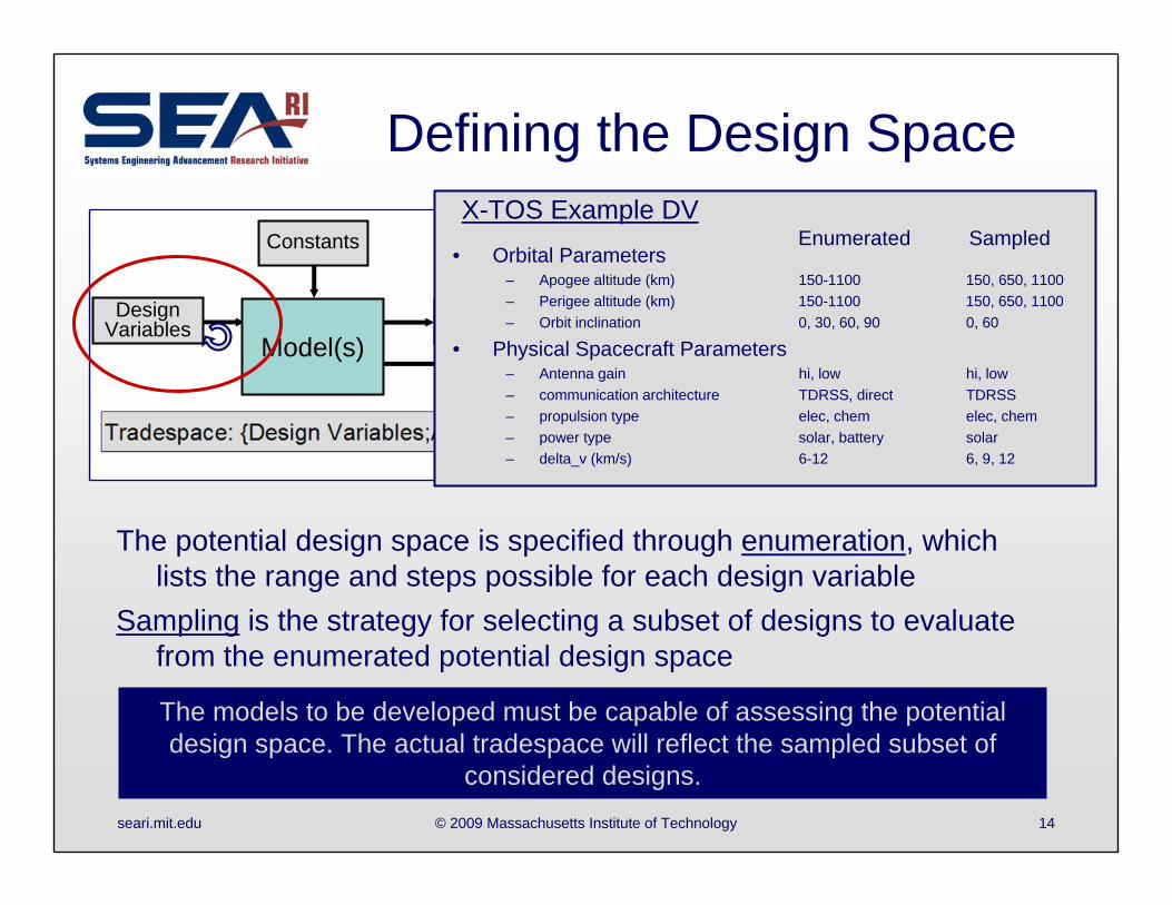
Defining the Design Space

The potential design space is specified through enumeration, which lists the range and steps possible for each design variable

Sampling is the strategy for selecting a subset of designs to evaluate from the enumerated potential design space

The models to be developed must be capable of assessing the potential design space. The actual tradespace will reflect the sampled subset of

considered designs.


Constants


Model(s)

• Orbital Parameters– Apogee altitude (km) 150-1100 150, 650, 1100 – Perigee altitude (km) 150-1100 150, 650, 1100– Orbit inclination 0, 30, 60, 90 0, 60

• Physical Spacecraft Parameters– Antenna gain hi, low hi, low– communication architecture TDRSS, direct TDRSS– propulsion type elec, chem elec, chem– power type solar, battery solar– delta_v (km/s) 6-12 6, 9, 12

Enumerated SampledX-TOS Example DV


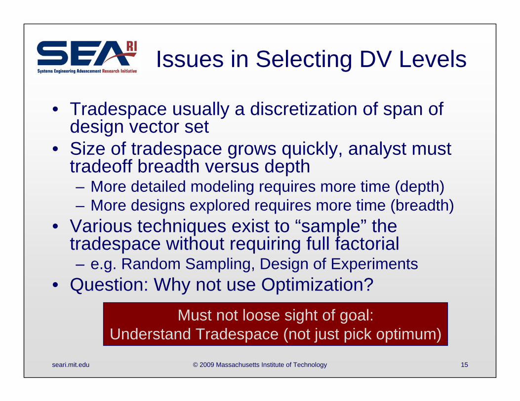
Issues in Selecting DV Levels

• Tradespace usually a discretization of span of design vector set

• Size of tradespace grows quickly, analyst must tradeoff breadth versus depth– More detailed modeling requires more time (depth)– More designs explored requires more time (breadth)

• Various techniques exist to “sample” the tradespace without requiring full factorial– e.g. Random Sampling, Design of Experiments

• Question: Why not use Optimization?Must not loose sight of goal:

Understand Tradespace (not just pick optimum)


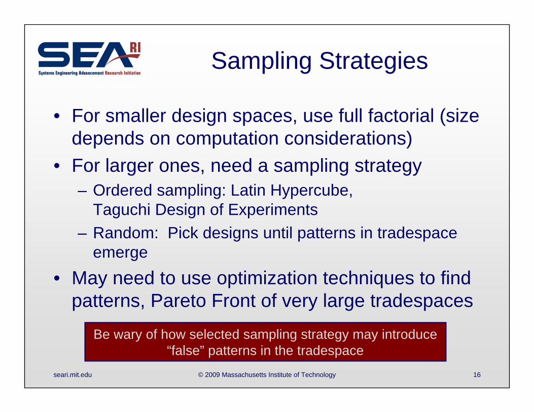
Sampling Strategies

• For smaller design spaces, use full factorial (size depends on computation considerations)

• For larger ones, need a sampling strategy– Ordered sampling: Latin Hypercube,

Taguchi Design of Experiments– Random: Pick designs until patterns in tradespace

emerge• May need to use optimization techniques to find

patterns, Pareto Front of very large tradespaces

Be wary of how selected sampling strategy may introduce “false” patterns in the tradespace


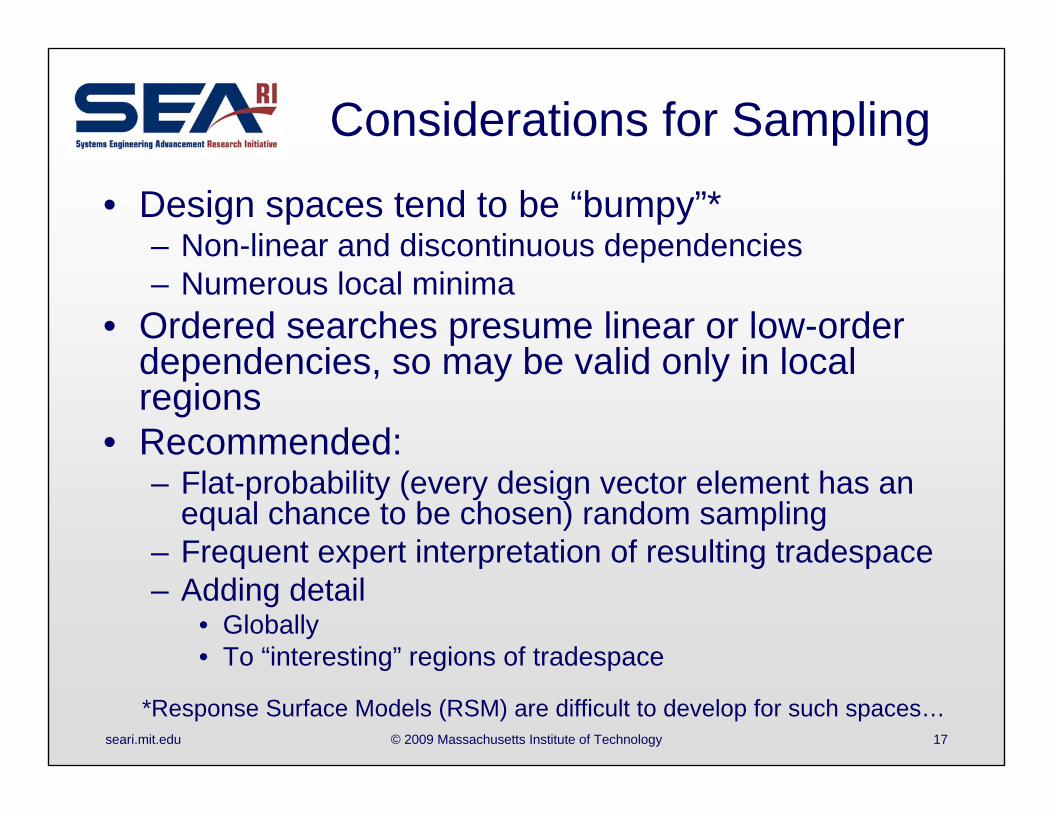
Considerations for Sampling

• Design spaces tend to be “bumpy”*– Non-linear and discontinuous dependencies– Numerous local minima

• Ordered searches presume linear or low-order dependencies, so may be valid only in local regions

• Recommended: – Flat-probability (every design vector element has an

equal chance to be chosen) random sampling– Frequent expert interpretation of resulting tradespace– Adding detail

• Globally• To “interesting” regions of tradespace

*Response Surface Models (RSM) are difficult to develop for such spaces…


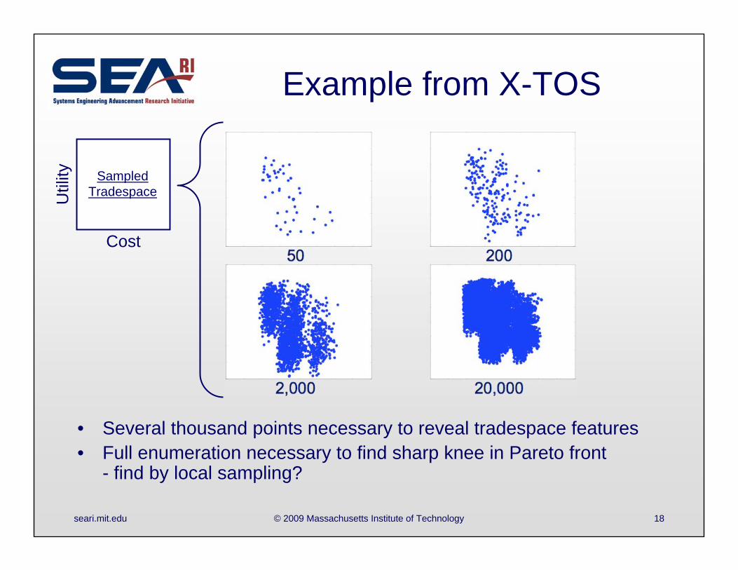
Example from X-TOS

• Several thousand points necessary to reveal tradespace features• Full enumeration necessary to find sharp knee in Pareto front

- find by local sampling?

Util

ity

Cost

Sampled Tradespace


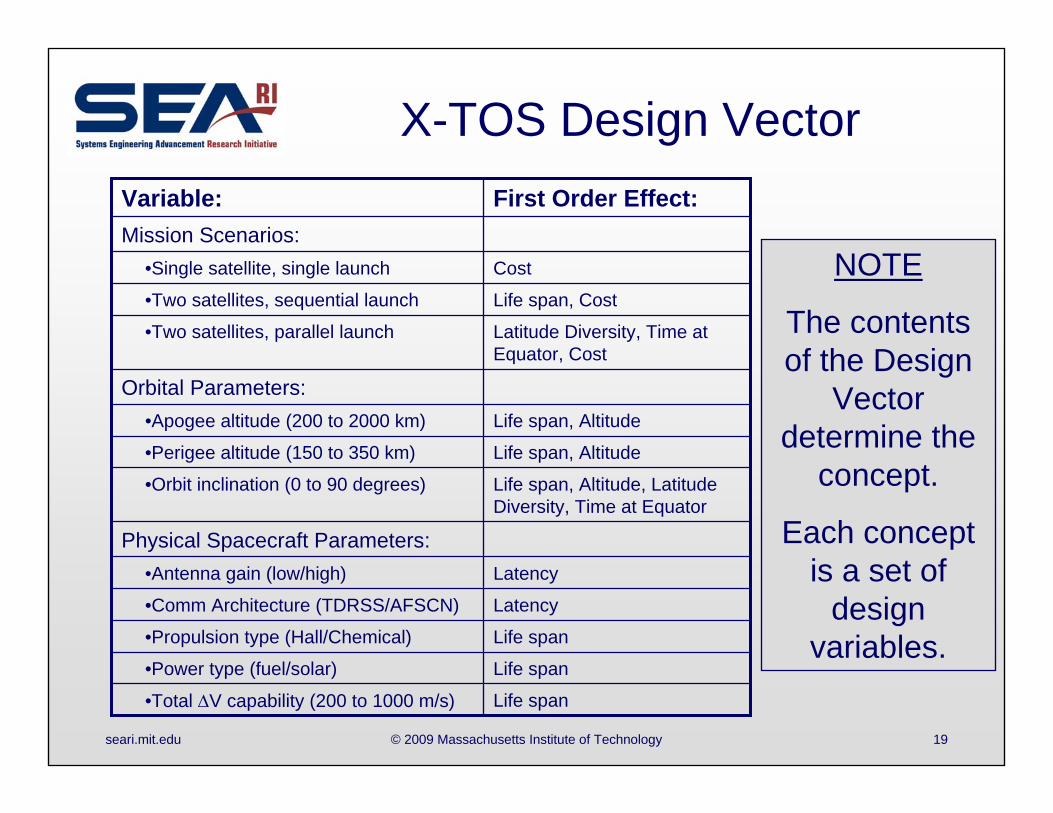
X-TOS Design Vector

Life span•Total V capability (200 to 1000 m/s)

Life span•Power type (fuel/solar)

Life span•Propulsion type (Hall/Chemical)

Latency•Comm Architecture (TDRSS/AFSCN)

Latency•Antenna gain (low/high)

Physical Spacecraft Parameters:

Life span, Altitude, Latitude Diversity, Time at Equator

•Orbit inclination (0 to 90 degrees)

Life span, Altitude•Perigee altitude (150 to 350 km)

Life span, Altitude•Apogee altitude (200 to 2000 km)

Orbital Parameters:

Latitude Diversity, Time at Equator, Cost

•Two satellites, parallel launch

Life span, Cost•Two satellites, sequential launch

Cost•Single satellite, single launch

Mission Scenarios:

First Order Effect:Variable:

NOTE

The contents of the Design

Vector determine the

concept.

Each concept is a set of

design variables.


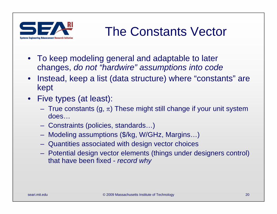
The Constants Vector

• To keep modeling general and adaptable to later changes, do not “hardwire” assumptions into code

• Instead, keep a list (data structure) where “constants” are kept

• Five types (at least):– True constants (g, ) These might still change if your unit system

does…– Constraints (policies, standards…)– Modeling assumptions ($/kg, W/GHz, Margins…)– Quantities associated with design vector choices – Potential design vector elements (things under designers control)

that have been fixed - record why


Defining the “Constants” Space

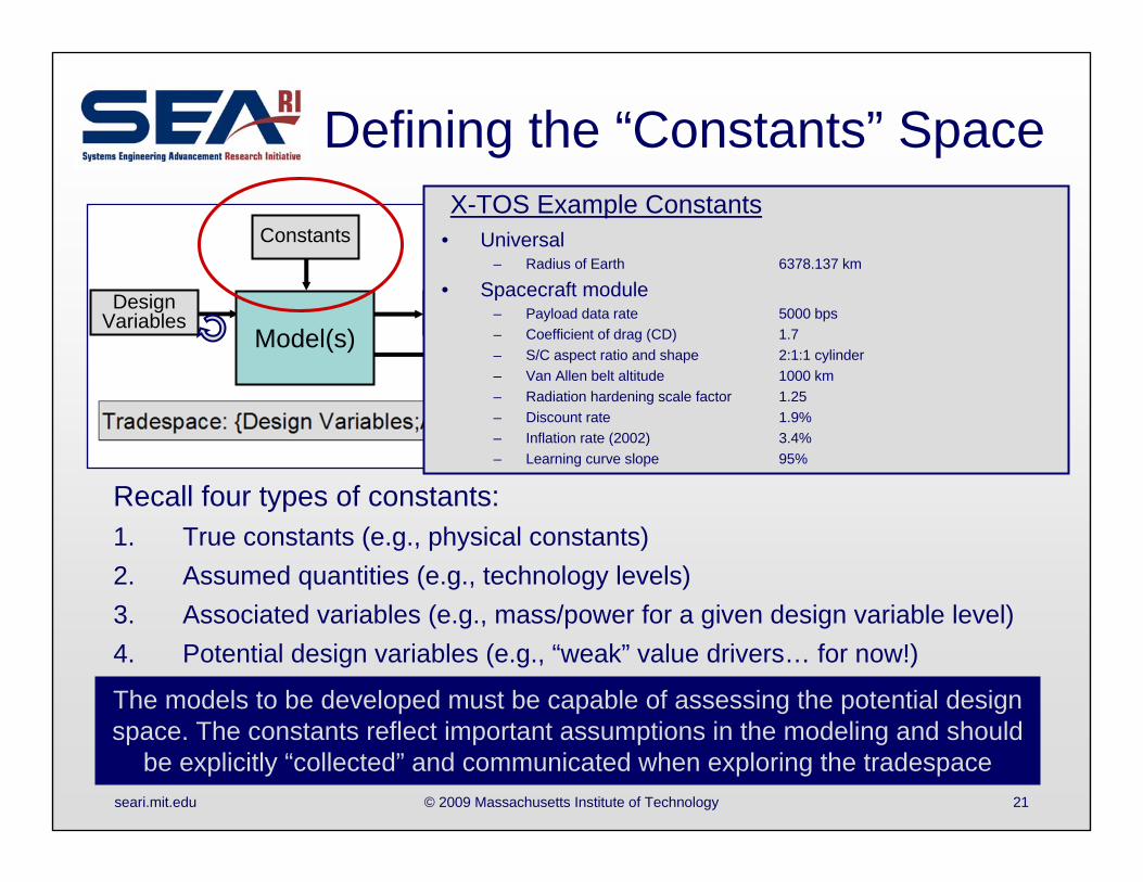
Recall four types of constants:1. True constants (e.g., physical constants)2. Assumed quantities (e.g., technology levels)3. Associated variables (e.g., mass/power for a given design variable level)4. Potential design variables (e.g., “weak” value drivers… for now!)

The models to be developed must be capable of assessing the potential design space. The constants reflect important assumptions in the modeling and should

be explicitly “collected” and communicated when exploring the tradespace


Constants


Model(s)

• Universal– Radius of Earth 6378.137 km

• Spacecraft module– Payload data rate 5000 bps– Coefficient of drag (CD) 1.7– S/C aspect ratio and shape 2:1:1 cylinder– Van Allen belt altitude 1000 km– Radiation hardening scale factor 1.25– Discount rate 1.9%– Inflation rate (2002) 3.4%– Learning curve slope 95%

X-TOS Example Constants


Modeling

Des

ign V

ars

Perigee

Apogee

Del

ta-V

Propuls

ion

Incl

inat

ion

Com

m S

yste

m

Ant.

Gai

n

Pow

er s

yste

m

Mis

sion S

cenar

io

Tota

l Im

pac

t

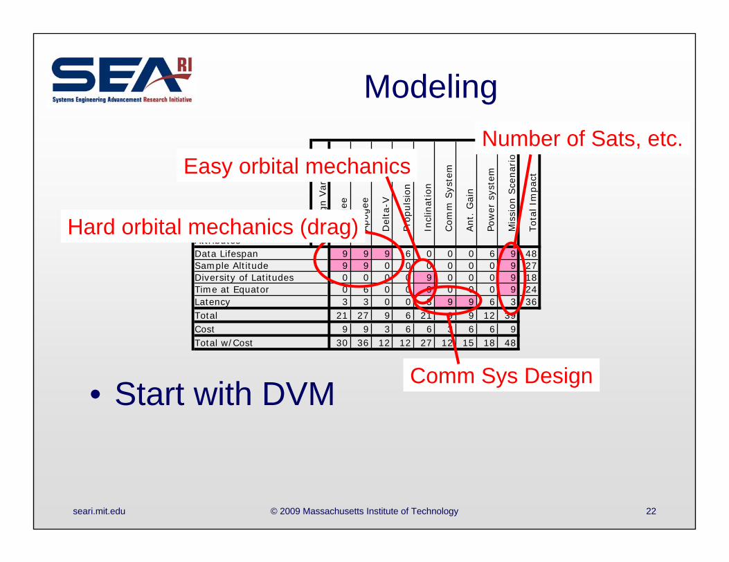
AttributesData Lifespan 9 9 9 6 0 0 0 6 9 48Sample Altitude 9 9 0 0 0 0 0 0 9 27Diversity of Latitudes 0 0 0 0 9 0 0 0 9 18Time at Equator 0 6 0 0 9 0 0 0 9 24Latency 3 3 0 0 3 9 9 6 3 36Total 21 27 9 6 21 9 9 12 39Cost 9 9 3 6 6 3 6 6 9Total w/Cost 30 36 12 12 27 12 15 18 48

• Start with DVM

Hard orbital mechanics (drag)

Easy orbital mechanics

Comm Sys Design

Number of Sats, etc.


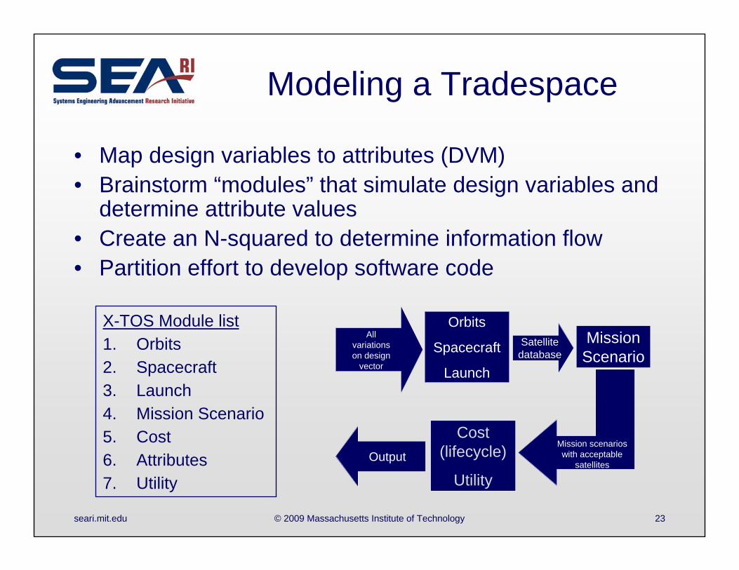
Modeling a Tradespace

• Map design variables to attributes (DVM)• Brainstorm “modules” that simulate design variables and

determine attribute values• Create an N-squared to determine information flow• Partition effort to develop software code

X-TOS Module list1. Orbits2. Spacecraft3. Launch4. Mission Scenario5. Cost6. Attributes7. Utility

Output

Satellitedatabase

Cost (lifecycle)

Utility

Mission Scenario

Orbits

Spacecraft

Launch

All variations on design

vector

Mission scenarios with acceptable

satellitesOutput

Satellitedatabase

Cost (lifecycle)

Utility

Mission Scenario

Orbits

Spacecraft

Launch

All variations on design

vector

Mission scenarios with acceptable

satellites


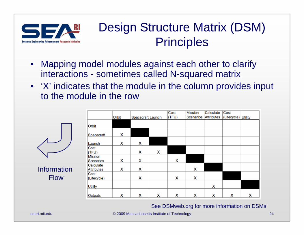
Design Structure Matrix (DSM) Principles

• Mapping model modules against each other to clarify interactions - sometimes called N-squared matrix

• ‘X’ indicates that the module in the column provides input to the module in the row

Information Flow

See DSMweb.org for more information on DSMs


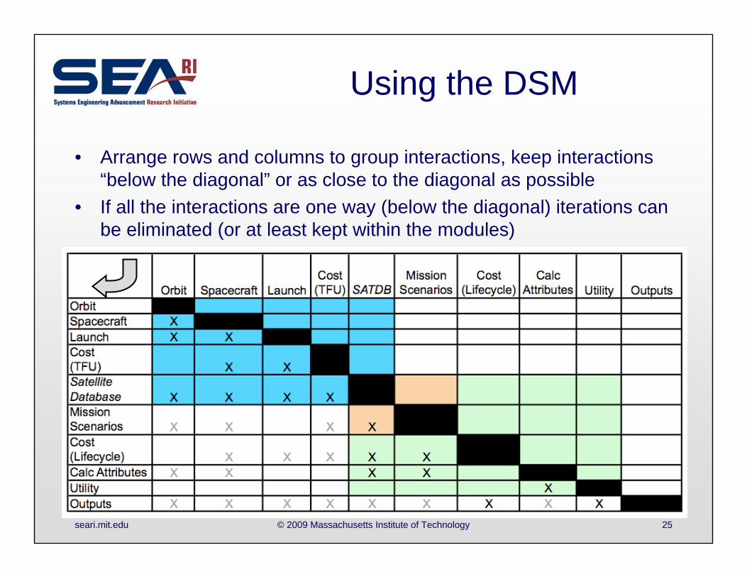
Using the DSM

• Arrange rows and columns to group interactions, keep interactions “below the diagonal” or as close to the diagonal as possible

• If all the interactions are one way (below the diagonal) iterations can be eliminated (or at least kept within the modules)


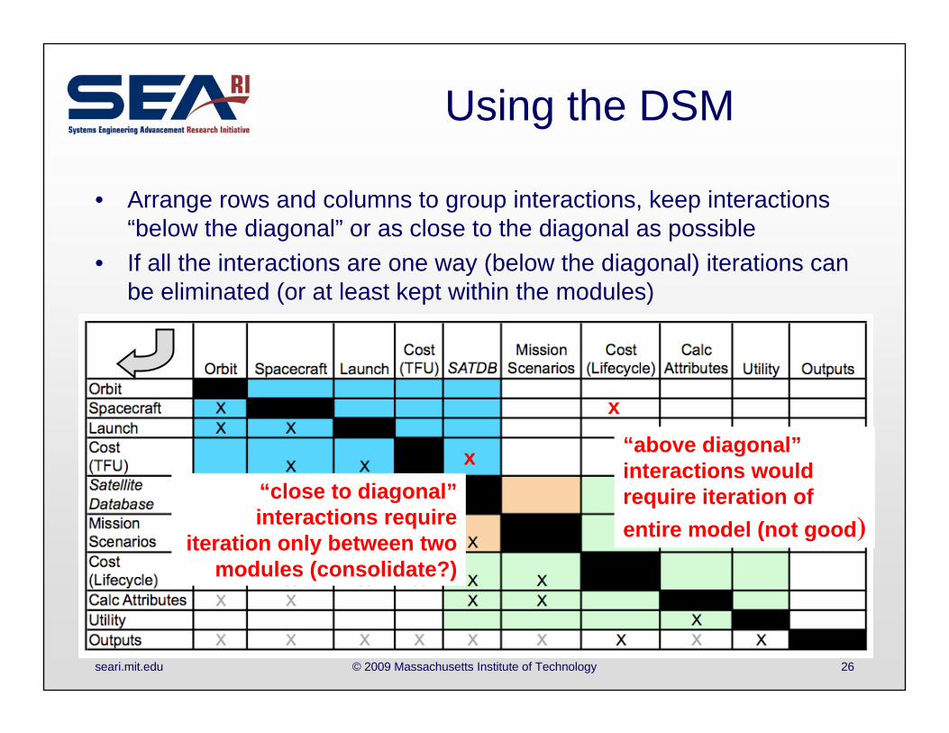
Using the DSM

• Arrange rows and columns to group interactions, keep interactions “below the diagonal” or as close to the diagonal as possible

• If all the interactions are one way (below the diagonal) iterations can be eliminated (or at least kept within the modules)

x

“above diagonal”interactions would require iteration of entire model (not good)

x“close to diagonal”interactions require

iteration only between two modules (consolidate?)


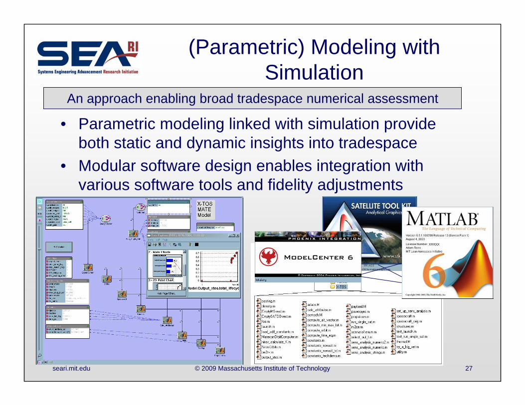
(Parametric) Modeling with Simulation

• Parametric modeling linked with simulation provide both static and dynamic insights into tradespace

• Modular software design enables integration with various software tools and fidelity adjustments

An approach enabling broad tradespace numerical assessment


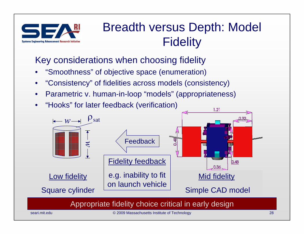
Breadth versus Depth: Model Fidelity

Key considerations when choosing fidelity• “Smoothness” of objective space (enumeration)• “Consistency” of fidelities across models (consistency)• Parametric v. human-in-loop “models” (appropriateness)• “Hooks” for later feedback (verification)

w

w

sat

Low fidelity

Square cylinderAll dimensions in meters

Mid fidelity

Simple CAD model

Feedback

Fidelity feedback

e.g. inability to fit on launch vehicle

Appropriate fidelity choice critical in early design


Cost Modeling:Criteria for selecting an Estimating Approach

• Have a balance of– Statistical significance (i.e., good fit to the data)– Practical significance (i.e., intuitively appealing cost drivers)

• Explainable to management– Defensible to skeptics– Reliable enough to justify $M or $B commitments

• General approaches are categorized as– Analogy– Parametric– Bottoms up/Engineering buildup– Extrapolation– Expert opinion (including usage of Delphi method)– Cost factors


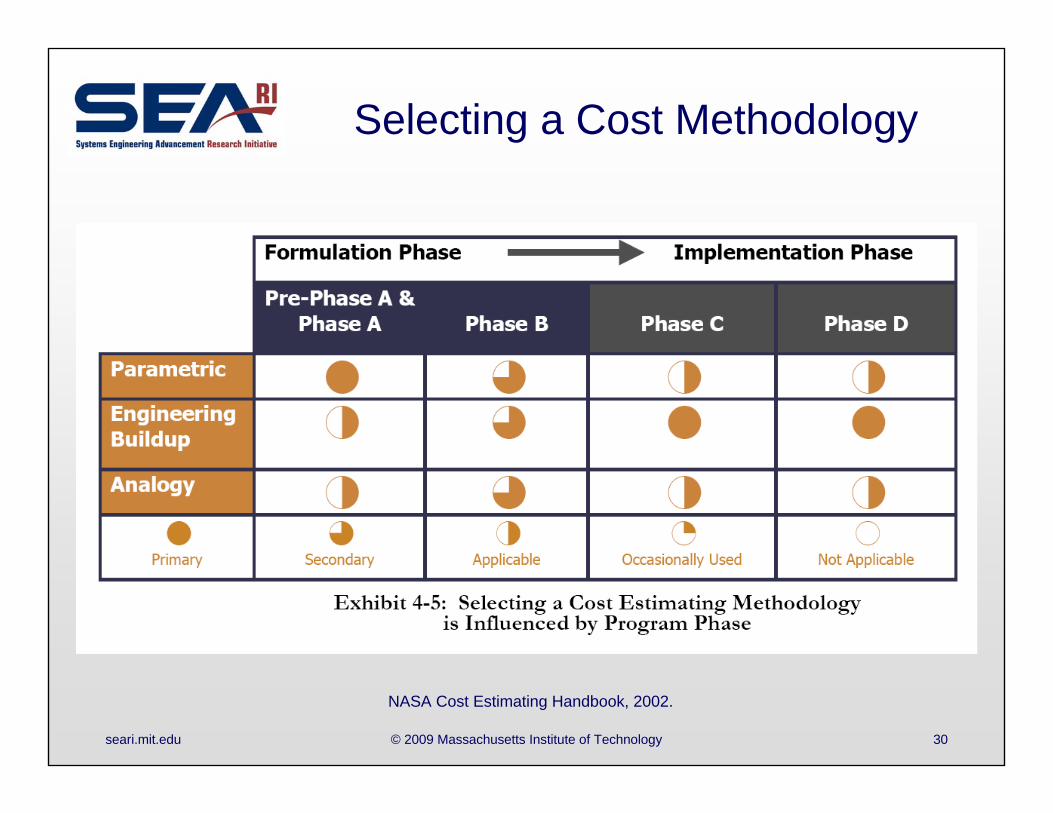
Selecting a Cost Methodology

NASA Cost Estimating Handbook, 2002.


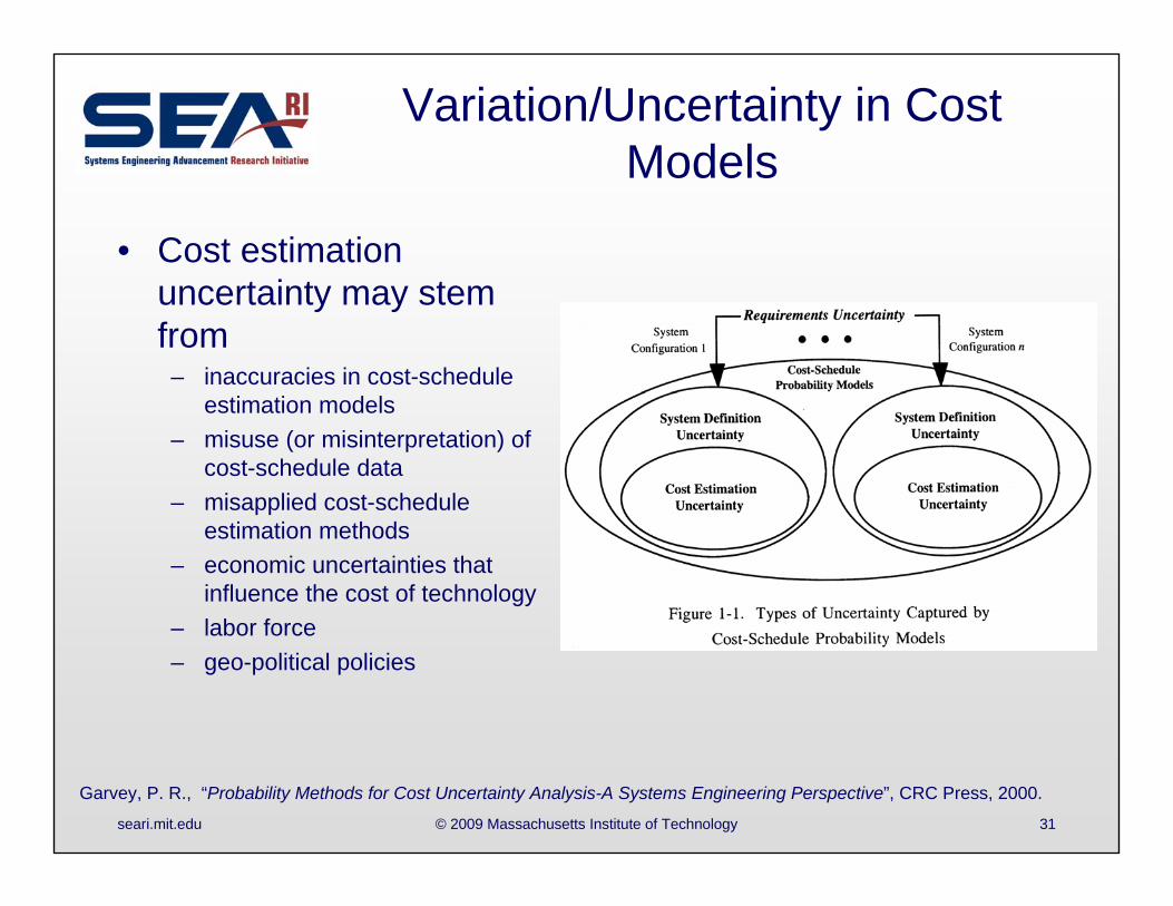
Variation/Uncertainty in Cost Models

• Cost estimation uncertainty may stem from

– inaccuracies in cost-schedule estimation models

– misuse (or misinterpretation) of cost-schedule data

– misapplied cost-schedule estimation methods

– economic uncertainties that influence the cost of technology

– labor force– geo-political policies

Garvey, P. R., “Probability Methods for Cost Uncertainty Analysis-A Systems Engineering Perspective”, CRC Press, 2000.


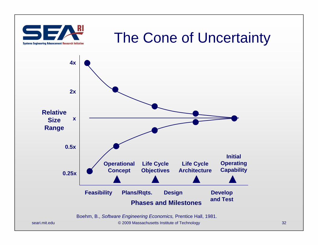
The Cone of Uncertainty

Feasibility Plans/Rqts. Design Develop and TestPhases and Milestones

Relative Size

Range

OperationalConcept

Life Cycle Objectives

Life Cycle Architecture

Initial Operating Capability

x

0.5x

0.25x

4x

2x

Boehm, B., Software Engineering Economics, Prentice Hall, 1981.


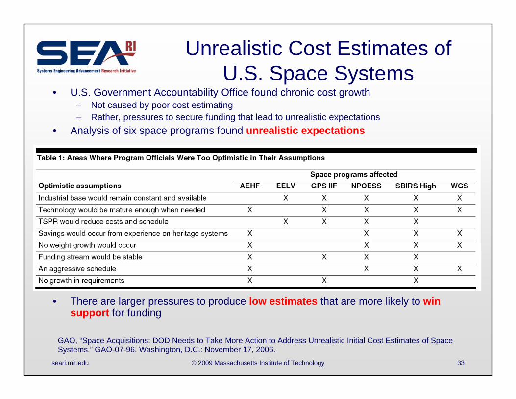
Unrealistic Cost Estimates of U.S. Space Systems

• U.S. Government Accountability Office found chronic cost growth– Not caused by poor cost estimating– Rather, pressures to secure funding that lead to unrealistic expectations

• Analysis of six space programs found unrealistic expectations

• There are larger pressures to produce low estimates that are more likely to win support for funding

GAO, “Space Acquisitions: DOD Needs to Take More Action to Address Unrealistic Initial Cost Estimates of SpaceSystems,” GAO-07-96, Washington, D.C.: November 17, 2006.


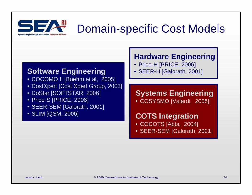
Domain-specific Cost Models

Software Engineering• COCOMO II [Boehm et al, 2005]• CostXpert [Cost Xpert Group, 2003]• CoStar [SOFTSTAR, 2006]• Price-S [PRICE, 2006]• SEER-SEM [Galorath, 2001]• SLIM [QSM, 2006]

Systems Engineering• COSYSMO [Valerdi, 2005]

COTS Integration• COCOTS [Abts, 2004]• SEER-SEM [Galorath, 2001]

Hardware Engineering• Price-H [PRICE, 2006]• SEER-H [Galorath, 2001]


Model Verification

• Good software practices - make sure code works

• Check sensitivities to both design vector and constants vector elements– Verify both model and assumptions (e.g. if results are

very sensitive to constants vector elements, reconsider assumptions)

– Discussed in tradespace exploration• Verify against more detailed analysis if available

– Conventional studies– Real products– ICE studies


Coupled with Tradespace Exploration

More techniques, coupled to issues of modeling:• Examining the effects of uncertainty in “constants”• Uncertainty in user needs and interaction with users• Basic confidence check - Does MATE yield realistic

results?

Remember ultimate goal: turn data generated by model into knowledge for decisions makers.

In addition, generate confidence in model and understandings of its limits

The goal here is to get a feeling for models to verify they produce “reasonable” results before proceeding to deeper tradespace exploration


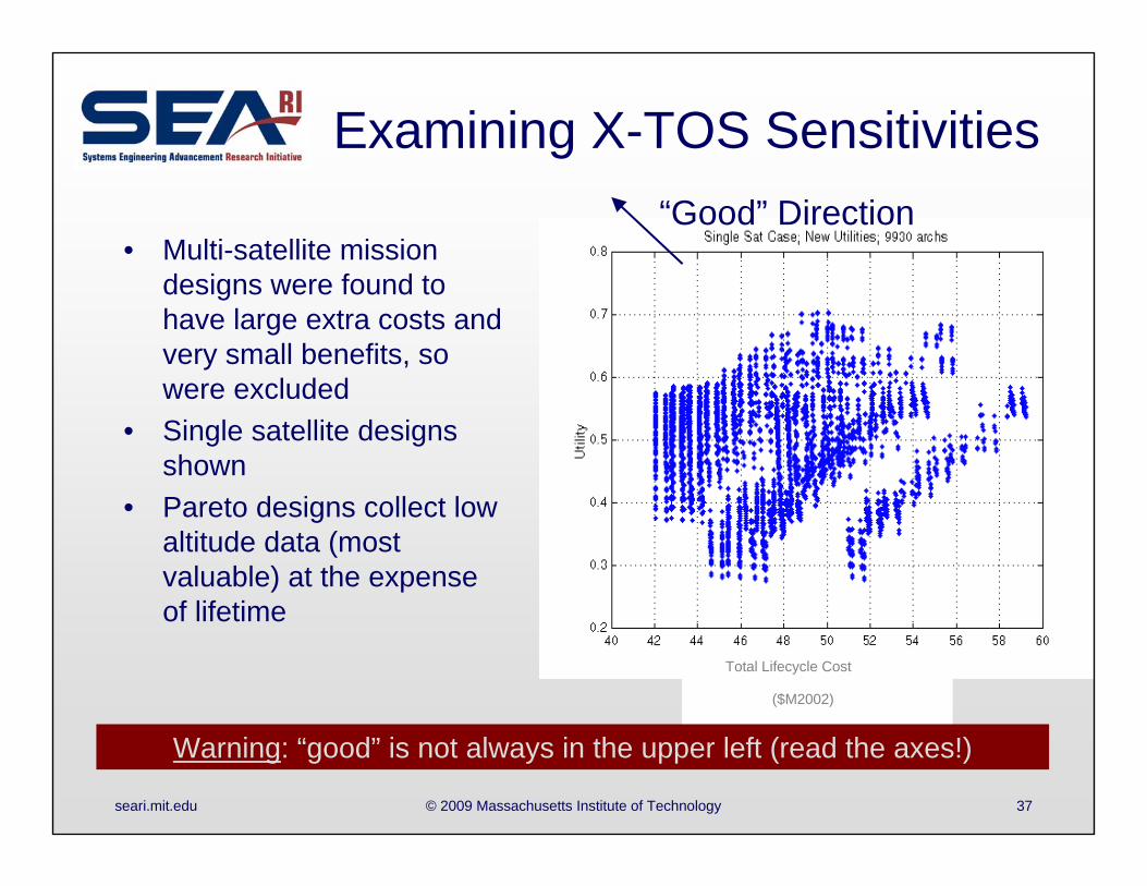
Examining X-TOS Sensitivities

Total Lifecycle Cost

($M2002)

• Multi-satellite mission designs were found to have large extra costs and very small benefits, so were excluded

• Single satellite designs shown

• Pareto designs collect low altitude data (most valuable) at the expense of lifetime

Warning: “good” is not always in the upper left (read the axes!)

“Good” Direction


Examining X-TOS Sensitivities

Total Lifecycle Cost

($M2002)

• Multi-satellite mission designs were found to have large extra costs and very small benefits, so were excluded

• Single satellite designs shown

• Pareto designs collect low altitude data (most valuable) at the expense of lifetime

Each point is a specific design

Pareto Front of “best”designs “Dominated”

designs are inferior in cost or utility

Warning: “good” is not always in the upper left (read the axes!)

“Good” Direction


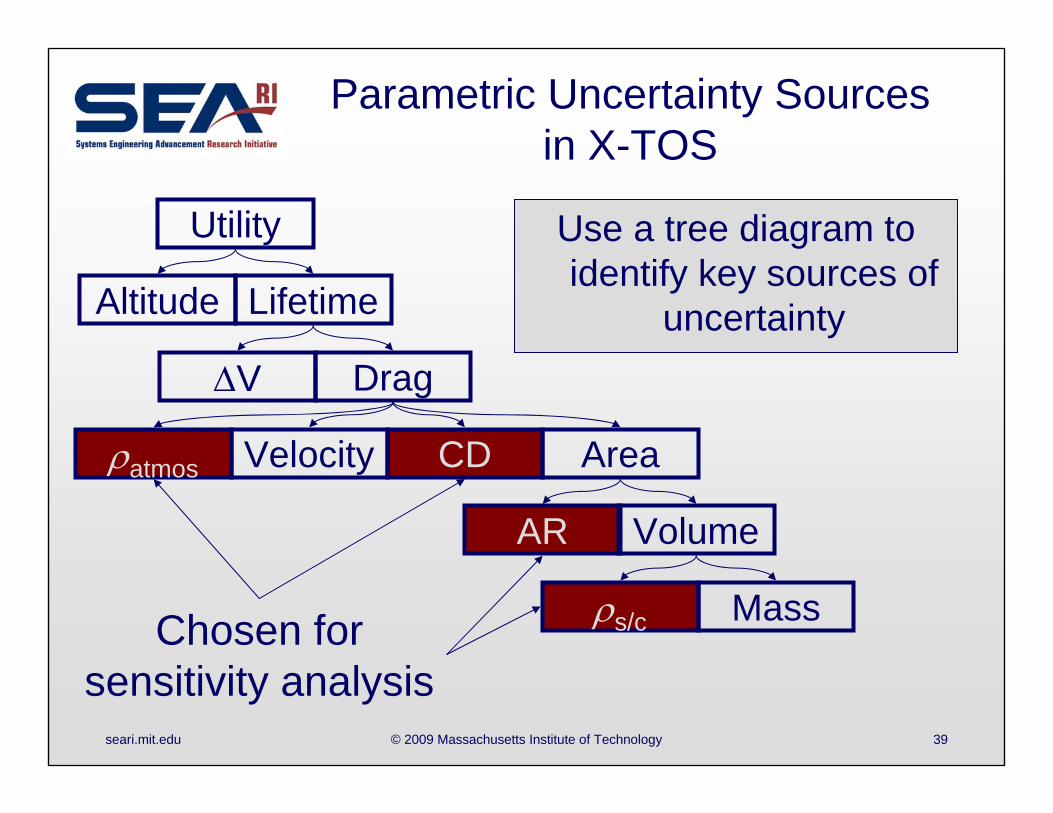
Parametric Uncertainty Sourcesin X-TOS

Use a tree diagram to identify key sources of

uncertainty

Utility

Altitude Lifetime

V Drag

atmos CDVelocity Area

AR Volume

s/c MassChosen for sensitivity analysis


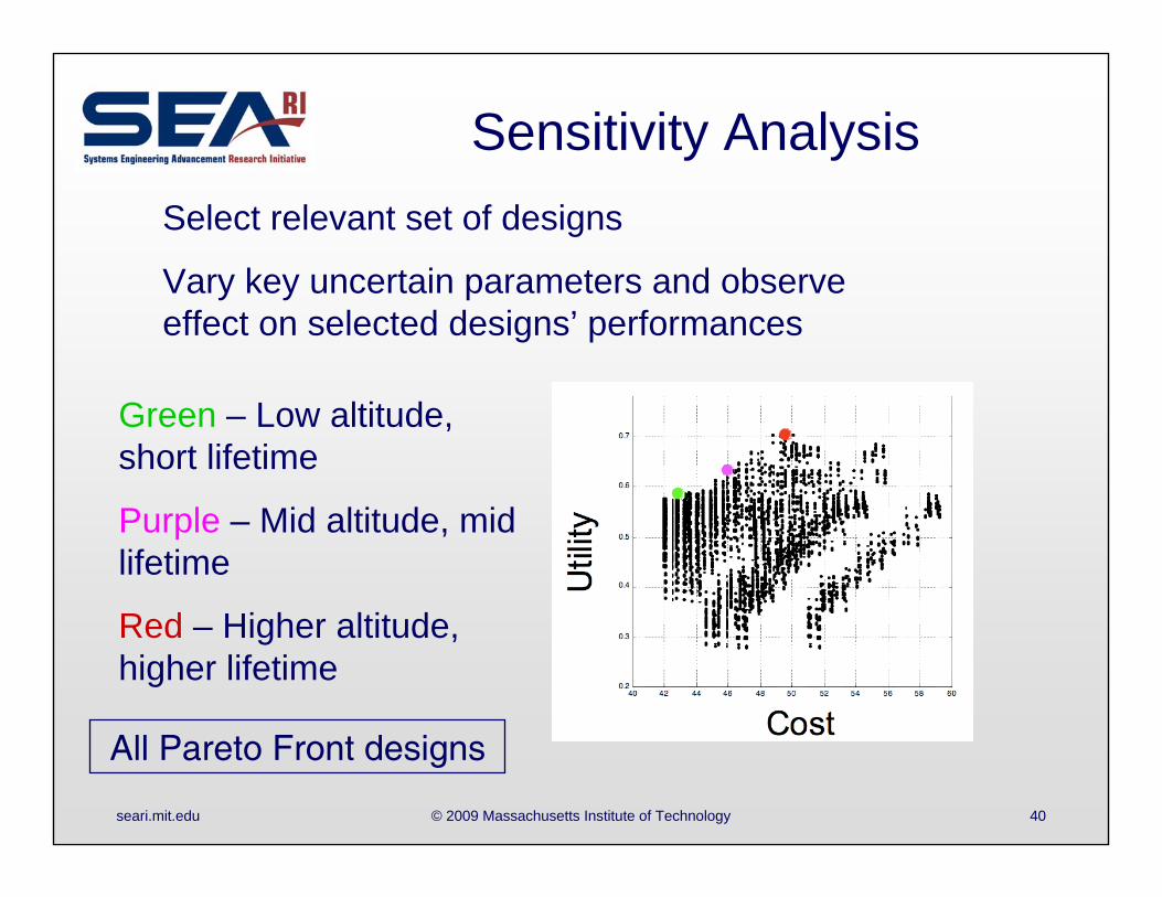
Sensitivity AnalysisSelect relevant set of designs

Vary key uncertain parameters and observe effect on selected designs’ performances

All Pareto Front designs

Green – Low altitude, short lifetime

Purple – Mid altitude, mid lifetime

Red – Higher altitude, higher lifetime


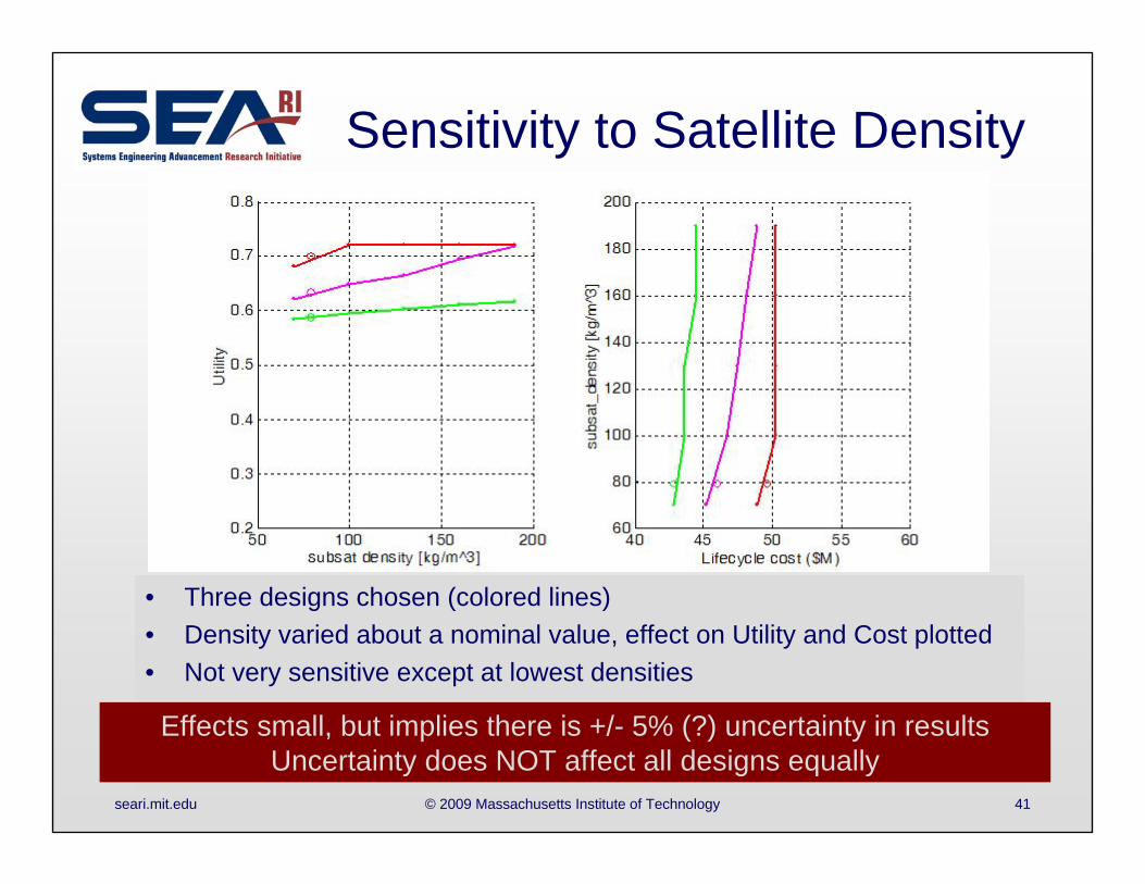
Sensitivity to Satellite Density

• Three designs chosen (colored lines)• Density varied about a nominal value, effect on Utility and Cost plotted• Not very sensitive except at lowest densities

Effects small, but implies there is +/- 5% (?) uncertainty in resultsUncertainty does NOT affect all designs equally


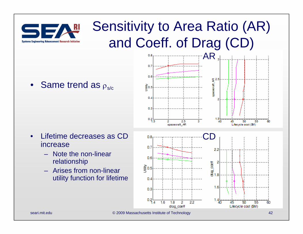
Sensitivity to Area Ratio (AR) and Coeff. of Drag (CD)

• Same trend as s/c

• Lifetime decreases as CD increase– Note the non-linear

relationship– Arises from non-linear

utility function for lifetime

AR

CD


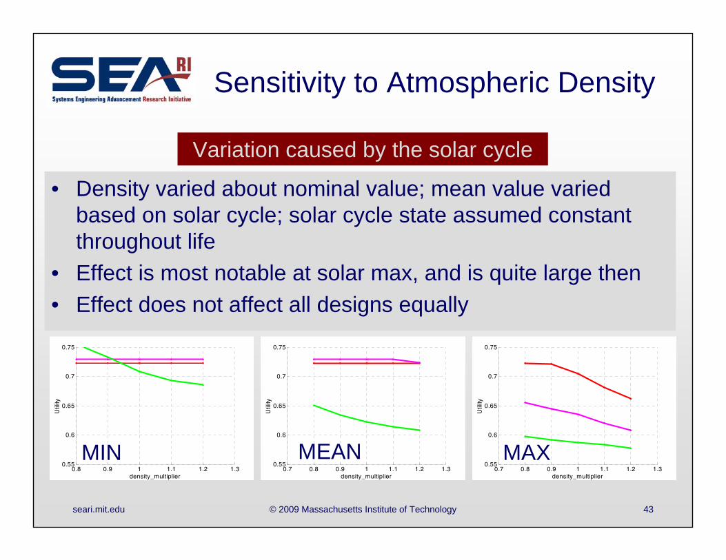
Sensitivity to Atmospheric Density

• Density varied about nominal value; mean value varied based on solar cycle; solar cycle state assumed constant throughout life

• Effect is most notable at solar max, and is quite large then• Effect does not affect all designs equally

Variation caused by the solar cycle

0.7 0.8 0.9 1 1.1 1.2 1.30.55

0.6

0.65

0.7

0.75

Util

itydensity_multiplier

0.7 0.8 0.9 1 1.1 1.2 1.30.55

0.6

0.65

0.7

0.75

Util

ity

density_multiplier0.8 0.9 1 1.1 1.2 1.3

0.55

0.6

0.65

0.7

0.75

Util

ity

density_multiplier

MIN MEAN MAX


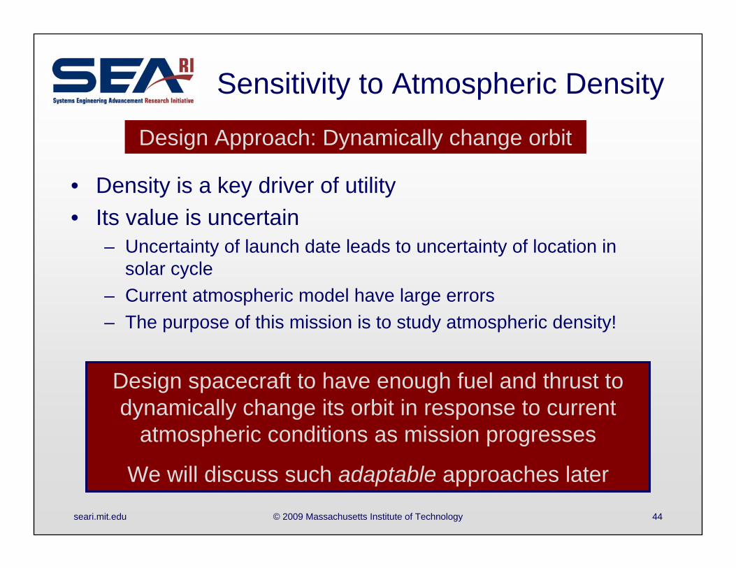
Sensitivity to Atmospheric Density

• Density is a key driver of utility• Its value is uncertain

– Uncertainty of launch date leads to uncertainty of location in solar cycle

– Current atmospheric model have large errors– The purpose of this mission is to study atmospheric density!

Design spacecraft to have enough fuel and thrust to dynamically change its orbit in response to current

atmospheric conditions as mission progresses

We will discuss such adaptable approaches later

Design Approach: Dynamically change orbit


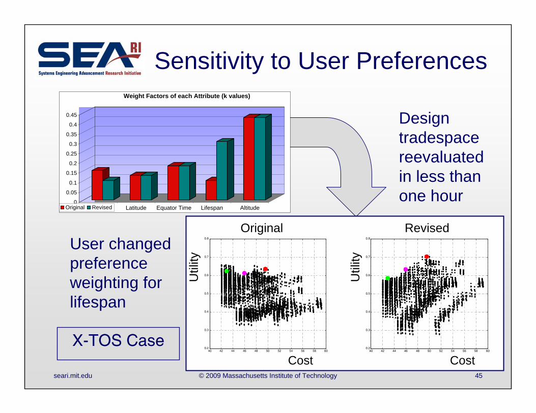
Sensitivity to User Preferences

User changed preference weighting for lifespan

Design tradespace reevaluated in less than one hour

X-TOS Case

0

0.05

0.1

0.15

0.2

0.25

0.3

0.35

0.4

0.45

Latency Latitude Equator Time Lifespan Altitude

Weight Factors of each Attribute (k values)

Original Revised

40 42 44 46 48 50 52 54 56 58 600.2

0.3

0.4

0.5

0.6

0.7

0.8

40 42 44 46 48 50 52 54 56 58 600.2

0.3

0.4

0.5

0.6

0.7

0.8

Original Revised

Util

ity

Util

ityCost Cost


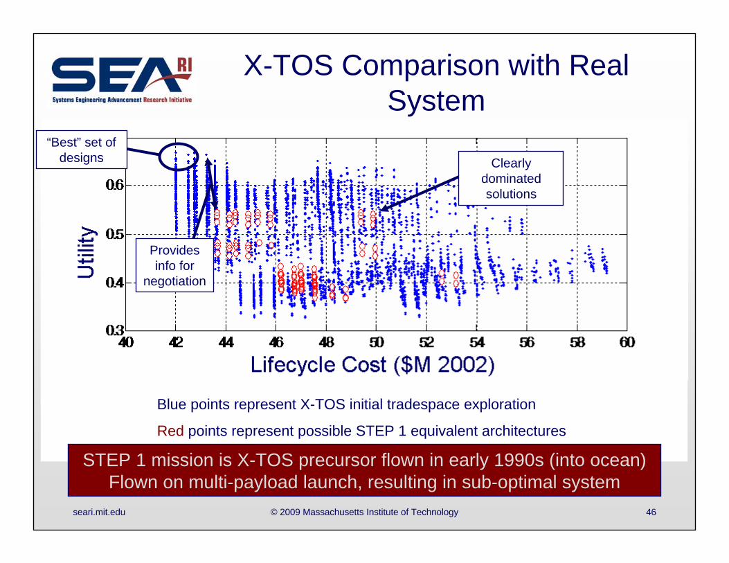
X-TOS Comparison with Real System

Blue points represent X-TOS initial tradespace exploration

Red points represent possible STEP 1 equivalent architectures

Important: Convert points back to attribute values for communicationSTEP 1 mission is X-TOS precursor flown in early 1990s (into ocean)Flown on multi-payload launch, resulting in sub-optimal system

Clearly dominated solutions

Provides info for

negotiation

“Best” set of designs


Total Lifecycle Cost($M2002)

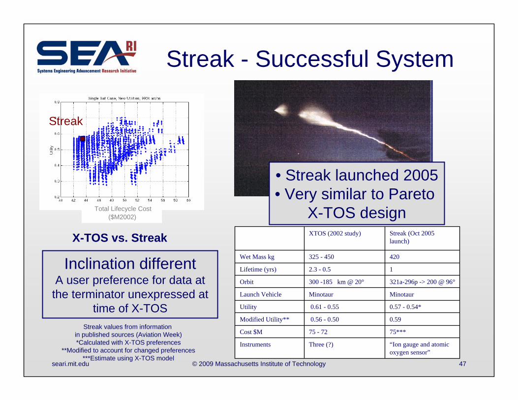
Streak - Successful System

X-TOS vs. Streak

“Ion gauge and atomic oxygen sensor”

Three (?)Instruments

75***75 - 72Cost $M

0.590.56 - 0.50 Modified Utility**

0.57 - 0.54*0.61 - 0.55 Utility

MinotaurMinotaurLaunch Vehicle

321a-296p -> 200 @ 96°300 -185 km @ 20°Orbit

12.3 - 0.5Lifetime (yrs)

420325 - 450Wet Mass kg

Streak (Oct 2005 launch)

XTOS (2002 study)

Streak

Inclination different A user preference for data at the terminator unexpressed at

time of X-TOS

• Streak launched 2005• Very similar to Pareto

X-TOS design

Streak values from information in published sources (Aviation Week)*Calculated with X-TOS preferences

**Modified to account for changed preferences***Estimate using X-TOS model


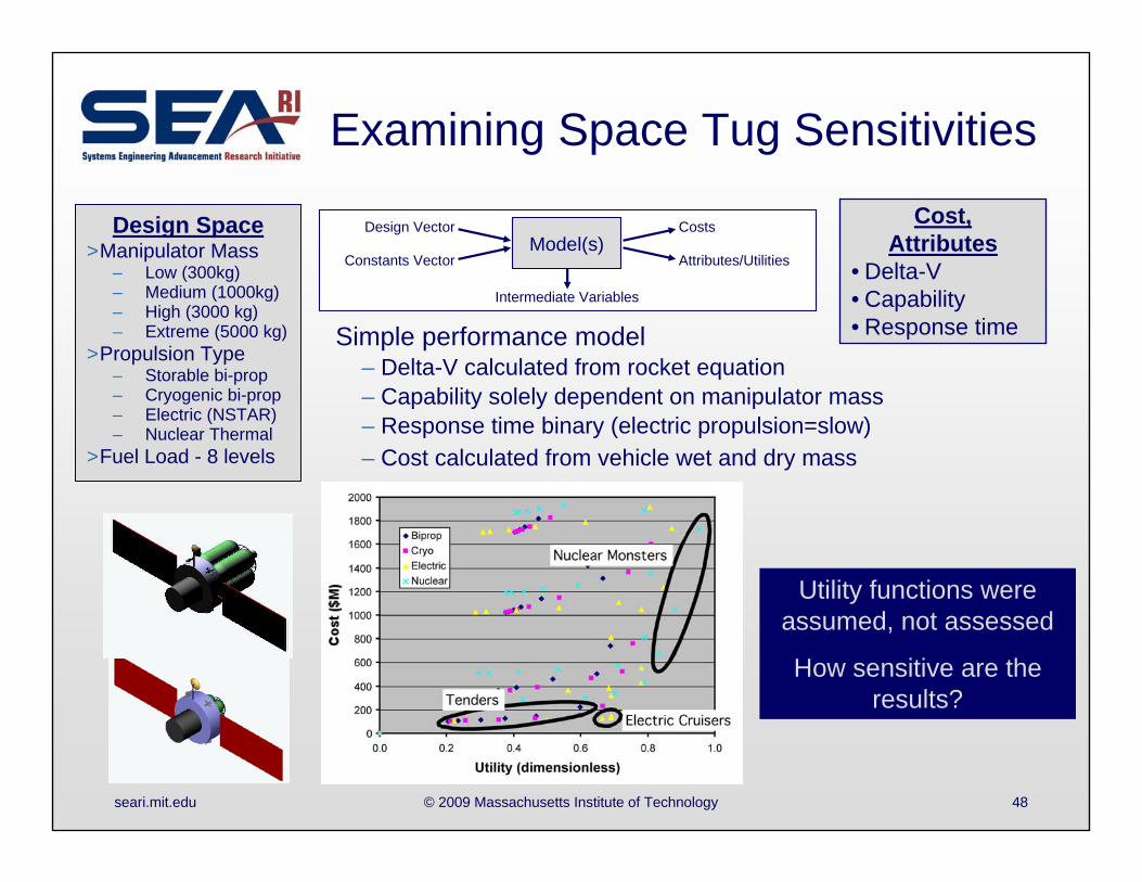
Cost,Attributes

• Delta-V• Capability• Response time

Design Space>Manipulator Mass

– Low (300kg)– Medium (1000kg)– High (3000 kg)– Extreme (5000 kg)

>Propulsion Type– Storable bi-prop– Cryogenic bi-prop– Electric (NSTAR)– Nuclear Thermal

>Fuel Load - 8 levels

Simple performance model– Delta-V calculated from rocket equation– Capability solely dependent on manipulator mass– Response time binary (electric propulsion=slow)– Cost calculated from vehicle wet and dry mass

Examining Space Tug Sensitivities

Design Vector

Constants VectorModel(s)

Costs

Attributes/Utilities

Intermediate Variables

Utility functions were assumed, not assessed

How sensitive are the results?


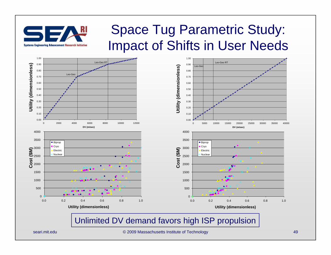
Space Tug Parametric Study:Impact of Shifts in User Needs

Unlimited DV demand favors high ISP propulsion

0.00

0.10

0.20

0.30

0.40

0.50

0.60

0.70

0.80

0.90

1.00

0 2000 4000 6000 8000 10000 12000

DV (m/sec)

Leo-Geo

Leo-Geo RT

0

500

1000

1500

2000

2500

3000

3500

4000

0.0 0.2 0.4 0.6 0.8 1.0

Utility (dimensionless)

Biprop CryoElectricNuclear

0.00

0.10

0.20

0.30

0.40

0.50

0.60

0.70

0.80

0.90

1.00

0 5000 10000 15000 20000 25000 30000 35000 40000

DV (m/sec)

Leo-GeoLeo-Geo RT

0

500

1000

1500

2000

2500

3000

3500

4000

0.0 0.2 0.4 0.6 0.8 1.0



Cos

t ($M

)

Cos

t ($M

)

Util

ity (d

imen

sion

less

)

Util

ity (d

imen

sion

less

)


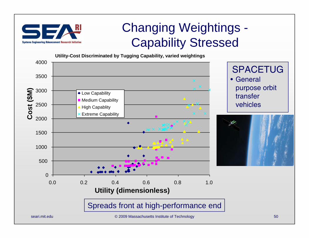
0

500

1000

1500

2000

2500

3000

3500

4000

0.0 0.2 0.4 0.6 0.8 1.0

Low Capability Medium CapabilityHigh CapablityExtreme Capability

Changing Weightings -Capability Stressed

Spreads front at high-performance end

SPACETUG• General

purpose orbit transfer vehicles

Cos

t ($M

)


Utility-Cost Discriminated by Tugging Capability, varied weightings


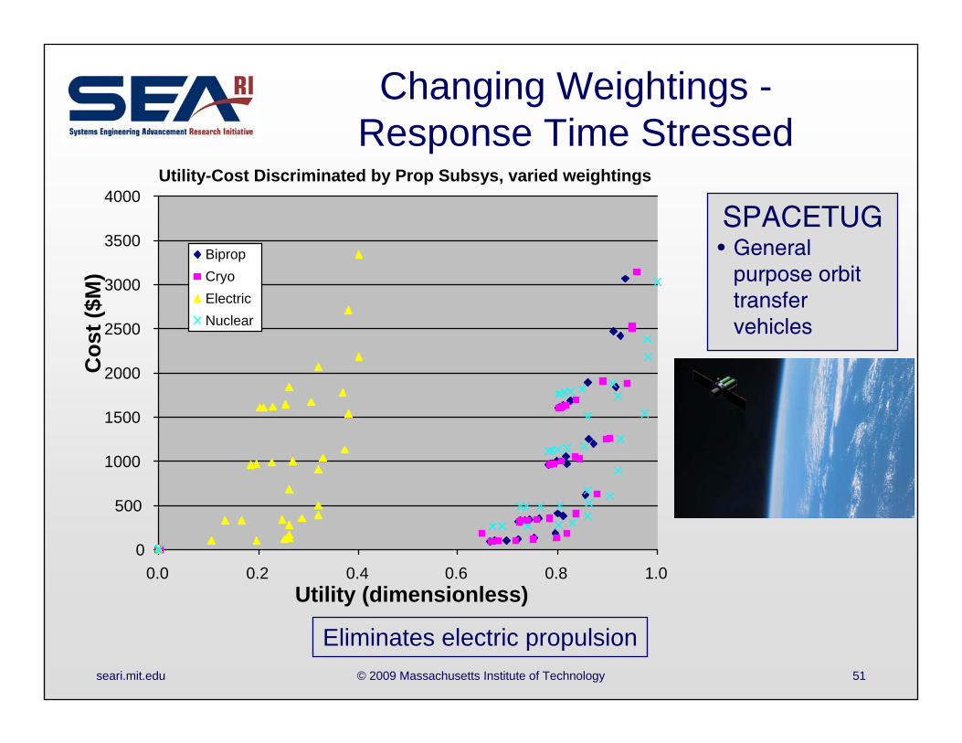
Changing Weightings -Response Time Stressed

Eliminates electric propulsion

0

500

1000

1500

2000

2500

3000

3500

4000

0.0 0.2 0.4 0.6 0.8 1.0


SPACETUG• General

purpose orbit transfer vehicles

Cos

t ($M

)


Utility-Cost Discriminated by Prop Subsys, varied weightings


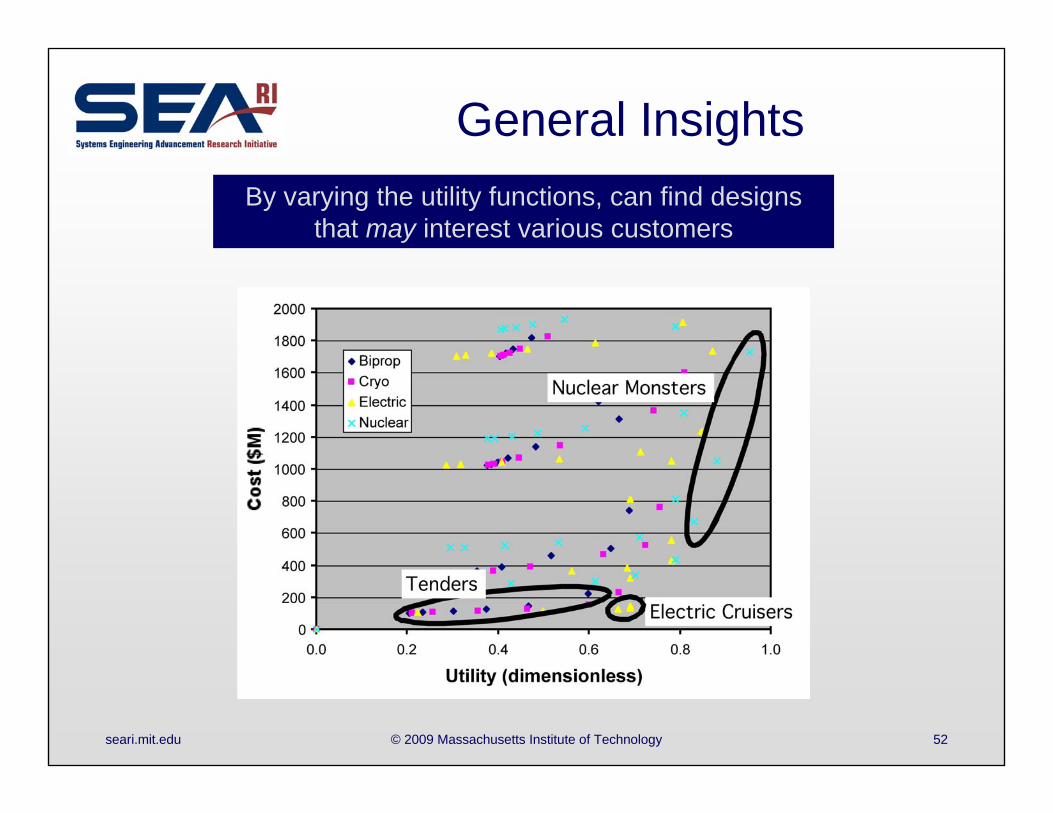
General InsightsBy varying the utility functions, can find designs

that may interest various customers


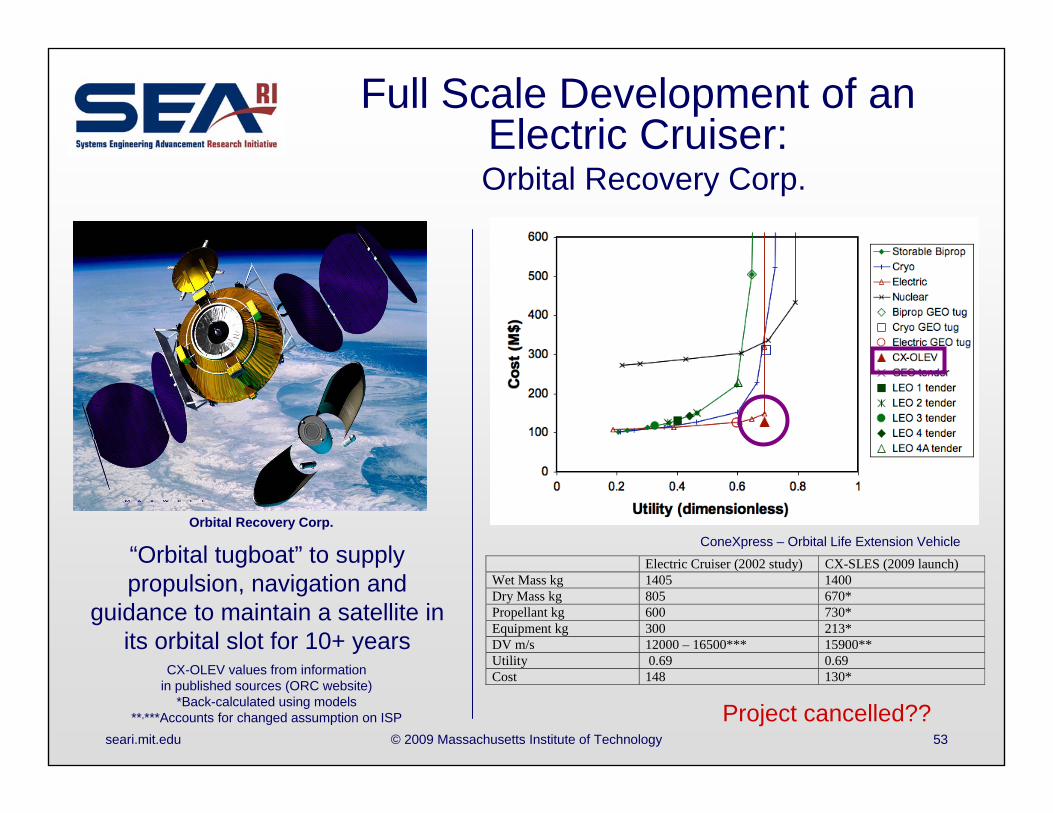
Full Scale Development of an Electric Cruiser:Orbital Recovery Corp.

Orbital Recovery Corp.

“Orbital tugboat” to supply propulsion, navigation and

guidance to maintain a satellite in its orbital slot for 10+ years

Electric Cruiser (2002 study) CX-SLES (2009 launch) Wet Mass kg 1405 1400 Dry Mass kg 805 670* Propellant kg 600 730* Equipment kg 300 213* DV m/s 12000 – 16500*** 15900** Utility 0.69 0.69 Cost 148 130*

CX-OLEV values from information in published sources (ORC website)

*Back-calculated using models**,***Accounts for changed assumption on ISP Project cancelled??

ConeXpress – Orbital Life Extension Vehicle


Orbital Express:An Experimental Tender

Orbital Express (OE)

On-orbit validation of autonomous docking, refueling, component

swapping; focus on non-proprietary interfaces

Flown 2007

Utility

Cos

t ($M

)


Summary

• Modeling Techniques– Defining analysis modules– Designing analysis system– Cost modeling– Verification of models

• Related Tradespace Exploration Techniques– Understanding sensitivities in model and constants– Understanding sensitivities to DM needs– Comparing to real systems


References for Cost Models• Boehm, B., Abts, C., Brown, A. W., Chulani, S., Clark, B. K., Horowitz, E., Madachy, R., Reifer,

D., Steece, B., Software Cost Estimation with COCOMO II, Prentice Hall, New Jersey, 2000.• Cost Xpert Group, Inc. Cost Xpert 3.3 Users Manual. San Diego, CA: Cost Xpert Group, Inc.,

2003.• PRICE, Program Affordability Management, http://www.pricesystems.com• QSM, SLIM-Estimate, http://www.qsm.com/slim_estimate.html • Galorath, Inc. SEER-SEM Users Manual. www.galorath.com• SOFTSTAR, http://softstarsystems.com• Valerdi, R., The Constructive Systems Engineering Cost Model (COSYSMO), PhD Dissertation,

University of Southern California, May 2005.• Abts, C., Extending the COCOMO II Software Cost Model to Estimate Effort and Schedule for

Software Systems Using Commercial-Off-The-Shelf (COTS) Software Components: the COCOTS model, PhD Dissertation, University of Southern California, 2004.

• Space Systems Cost Analysis Group (http://sscag.saic.com/)• Wertz, J. R. and Larson, W. J. (Eds.), Space Mission Analysis and Design, 3rd Edition, Microcosm

Press and Kluwer Academic Publishing, 1999. (Chapter 20 - Cost Modeling)• International Society of Parametric Analysts (http://www.ispa-cost.org/)• Valerdi, R., Wheaton, M. J., Fortune, J., “Systems Engineering Cost Estimation for Space

Systems,” AIAA Space 2007.

seari short course series

Documents