Search for gravitational waves associated with the August 2006 timing glitch of the Vela pulsar

J. Abadie,17 B. P. Abbott,17 R. Abbott,17 R. Adhikari,17 P. Ajith,17 B. Allen,2,60 G. Allen,35 E. Amador Ceron,60

R. S. Amin,21 S. B. Anderson,17 W.G. Anderson,60 M.A. Arain,47 M. Araya,17 Y. Aso,17 S. Aston,46 P. Aufmuth,16

C. Aulbert,2 S. Babak,1 P. Baker,24 S. Ballmer,17 D. Barker,18 B. Barr,48 P. Barriga,59 L. Barsotti,20 M.A. Barton,18

I. Bartos,10 R. Bassiri,48 M. Bastarrika,48 B. Behnke,1 M. Benacquista,42 M. F. Bennett,38 J. Betzwieser,17

P. T. Beyersdorf,31 I. A. Bilenko,25 G. Billingsley,17 R. Biswas,60 E. Black,17 J. K. Blackburn,17 L. Blackburn,20 D. Blair,59

B. Bland,18 O. Bock,2 T. P. Bodiya,20 R. Bondarescu,37 R. Bork,17 M. Born,2 S. Bose,61 P. R. Brady,60 V. B. Braginsky,25

J. E. Brau,53 J. Breyer,2 D.O. Bridges,19 M. Brinkmann,2 M. Britzger,2 A. F. Brooks,17 D.A. Brown,36 A. Bullington,35

A. Buonanno,49 O. Burmeister,2 R. L. Byer,35 L. Cadonati,50 J. Cain,39 J. B. Camp,26 J. Cannizzo,26 K. C. Cannon,17

J. Cao,20 C. Capano,36 L. Cardenas,17 S. Caudill,21 M. Cavaglia,39 C. Cepeda,17 T. Chalermsongsak,17 E. Chalkley,48

P. Charlton,9 S. Chatterji,17 S. Chelkowski,46 Y. Chen,6 N. Christensen,8 S. S. Y. Chua,4 C. T. Y. Chung,38 D. Clark,35

J. Clark,7 J. H. Clayton,60 R. Conte,55 D. Cook,18 T. R. C. Corbitt,20 N. Cornish,24 D. Coward,59 D. C. Coyne,17

J. D. E. Creighton,60 T. D. Creighton,42 A.M. Cruise,46 R.M. Culter,46 A. Cumming,48 L. Cunningham,48 K. Dahl,2

S. L. Danilishin,25 K. Danzmann,2,16 B. Daudert,17 G. Davies,7 E. J. Daw,40 T. Dayanga,61 D. DeBra,35 J. Degallaix,2

V. Dergachev,51 R. DeSalvo,17 S. Dhurandhar,15 M. Dıaz,42 F. Donovan,20 K. L. Dooley,47 E. E. Doomes,34

R.W. P. Drever,5 J. Driggers,17 J. Dueck,2 I. Duke,20 J.-C. Dumas,59 M. Edgar,48 M. Edwards,7 A. Effler,18 P. Ehrens,17

T. Etzel,17 M. Evans,20 T. Evans,19 S. Fairhurst,7 Y. Faltas,47 Y. Fan,59 D. Fazi,17 H. Fehrmann,2 L. S. Finn,37 K. Flasch,60

S. Foley,20 C. Forrest,54 N. Fotopoulos,60 M. Frede,2 M. Frei,41 Z. Frei,12 A. Freise,46 R. Frey,53 T. T. Fricke,21

D. Friedrich,2 P. Fritschel,20 V. V. Frolov,19 P. Fulda,46 M. Fyffe,19 J. A. Garofoli,36 S. Ghosh,61 J. A. Giaime,21,19

S. Giampanis,2 K.D. Giardina,19 E. Goetz,51 L.M. Goggin,60 G. Gonzalez,21 S. Goßler,2 A. Grant,48 S. Gras,59 C. Gray,18

R. J. S. Greenhalgh,30 A.M. Gretarsson,11 R. Grosso,42 H. Grote,2 S. Grunewald,1 E. K. Gustafson,17 R. Gustafson,51

B. Hage,16 J.M. Hallam,46 D. Hammer,60 G. D. Hammond,48 C. Hanna,17 J. Hanson,19 J. Harms,52 G.M. Harry,20

I.W. Harry,7 E. D. Harstad,53 K. Haughian,48 K. Hayama,2 T. Hayler,30 J. Heefner,17 I. S. Heng,48 A. Heptonstall,17

M. Hewitson,2 S. Hild,46 E. Hirose,36 D. Hoak,19 K. A. Hodge,17 K. Holt,19 D. J. Hosken,45 J. Hough,48 E. Howell,59

D. Hoyland,46 B. Hughey,20 S. Husa,44 S. H. Huttner,48 D. R. Ingram,18 T. Isogai,8 A. Ivanov,17 W.W. Johnson,21

D. I. Jones,57 G. Jones,7 R. Jones,48 L. Ju,59 P. Kalmus,17 V. Kalogera,28 S. Kandhasamy,52 J. Kanner,49 E. Katsavounidis,20

K. Kawabe,18 S. Kawamura,27 F. Kawazoe,2 W. Kells,17 D. G. Keppel,17 A. Khalaidovski,2 F. Y. Khalili,25 R. Khan,10

E. Khazanov,14 H. Kim,2 P. J. King,17 J. S. Kissel,21 S. Klimenko,47 K. Kokeyama,27 V. Kondrashov,17 R. Kopparapu,37

S. Koranda,60 D. Kozak,17 V. Kringel,2 B. Krishnan,1 G. Kuehn,2 J. Kullman,2 R. Kumar,48 P. Kwee,16 P. K. Lam,4

M. Landry,18 M. Lang,37 B. Lantz,35 N. Lastzka,2 A. Lazzarini,17 P. Leaci,2 M. Lei,17 N. Leindecker,35 I. Leonor,53

H. Lin,47 P. E. Lindquist,17 T. B. Littenberg,24 N.A. Lockerbie,58 D. Lodhia,46 M. Lormand,19 P. Lu,35 M. Lubinski,18

A. Lucianetti,47 H. Luck,2,16 A. Lundgren,36 B. Machenschalk,2 M. MacInnis,20 M. Mageswaran,17 K. Mailand,17

C. Mak,17 I. Mandel,28 V. Mandic,52 S. Marka,10 Z. Marka,10 A. Markosyan,35 J. Markowitz,20 E. Maros,17 I.W. Martin,48

R.M. Martin,47 J. N. Marx,17 K. Mason,20 F. Matichard,20,21 L. Matone,10 R. A. Matzner,41 N. Mavalvala,20

R. McCarthy,18 D. E. McClelland,4 S. C. McGuire,34 G. McIntyre,17 D. J. A. McKechan,7 M. Mehmet,2 A. Melatos,38

A. C. Melissinos,54 G. Mendell,18 D. F. Menendez,37 R. A. Mercer,60 L. Merrill,59 S. Meshkov,17 C. Messenger,2

M. S. Meyer,19 H. Miao,59 J. Miller,48 Y. Mino,6 S. Mitra,17 V. P. Mitrofanov,25 G. Mitselmakher,47 R. Mittleman,20

O. Miyakawa,17 B. Moe,60 S. D. Mohanty,42 S. R. P. Mohapatra,50 G. Moreno,18 K. Mors,2 K. Mossavi,2 C. MowLowry,4

G. Mueller,47 H. Muller-Ebhardt,2 S. Mukherjee,42 A. Mullavey,4 J. Munch,45 P. G. Murray,48 T. Nash,17 R. Nawrodt,48

J. Nelson,48 G. Newton,48 E. Nishida,27 A. Nishizawa,27 J. O’Dell,30 B. O’Reilly,19 R. O’Shaughnessy,37 E. Ochsner,49

G.H. Ogin,17 R. Oldenburg,60 D. J. Ottaway,45 R. S. Ottens,47 H. Overmier,19 B. J. Owen,37 A. Page,46 Y. Pan,49

C. Pankow,47 M.A. Papa,1,60 P. Patel,17 D. Pathak,7 M. Pedraza,17 L. Pekowsky,36 S. Penn,13 C. Peralta,1 A. Perreca,46

M. Pickenpack,2 I.M. Pinto,56 M. Pitkin,48 H. J. Pletsch,2 M.V. Plissi,48 F. Postiglione,56 M. Principe,56 R. Prix,2

L. Prokhorov,25 O. Puncken,2 V. Quetschke,42 F. J. Raab,18 D. S. Rabeling,4 H. Radkins,18 P. Raffai,12 Z. Raics,10

M. Rakhmanov,42 V. Raymond,28 C.M. Reed,18 T. Reed,22 H. Rehbein,2 S. Reid,48 D.H. Reitze,47 R. Riesen,19 K. Riles,51

P. Roberts,3 N.A. Robertson,17,48 C. Robinson,7 E. L. Robinson,1 S. Roddy,19 C. Rover,2 J. Rollins,10 J. D. Romano,42

J. H. Romie,19 S. Rowan,48 A. Rudiger,2 K. Ryan,18 S. Sakata,27 L. Sammut,38 L. Sancho de la Jordana,44 V. Sandberg,18

V. Sannibale,17 L. Santamarıa,1 G. Santostasi,23 S. Saraf,32 P. Sarin,20 B. S. Sathyaprakash,7 S. Sato,27 M. Satterthwaite,4

P. R. Saulson,36 R. Savage,18 R. Schilling,2 R. Schnabel,2 R. Schofield,53 B. Schulz,2 B. F. Schutz,1,7 P. Schwinberg,18

J. Scott,48 S.M. Scott,4 A. C. Searle,17 F. Seifert,2,17 D. Sellers,19 A. S. Sengupta,17 A. Sergeev,14 B. Shapiro,20

PHYSICAL REVIEW D 83, 042001 (2011)

1550-7998=2011=83(4)=042001(13) 042001-1 � 2011 American Physical Society

P. Shawhan,49 D. H. Shoemaker,20 A. Sibley,19 X. Siemens,60 D. Sigg,18 A.M. Sintes,44 G. Skelton,60 B. J. J. Slagmolen,4

J. Slutsky,21 J. R. Smith,36 M. R. Smith,17 N.D. Smith,20 K. Somiya,6 B. Sorazu,48 F. Speirits,48 A. J. Stein,20 L. C. Stein,20

S. Steplewski,61 A. Stochino,17 R. Stone,42 K.A. Strain,48 S. Strigin,25 A. Stroeer,26 A. L. Stuver,19 T. Z. Summerscales,3

M. Sung,21 S. Susmithan,59 P. J. Sutton,7 G. P. Szokoly,12 D. Talukder,61 D. B. Tanner,47 S. P. Tarabrin,25 J. R. Taylor,2

R. Taylor,17 K.A. Thorne,19 K. S. Thorne,6 A. Thuring,16 C. Titsler,37 K.V. Tokmakov,48,58 C. Torres,19 C. I. Torrie,17,48

G. Traylor,19 M. Trias,44 L. Turner,17 D. Ugolini,43 K. Urbanek,35 H. Vahlbruch,16 M. Vallisneri,6 C. Van Den Broeck,7

M.V. van der Sluys,28 A. A. van Veggel,48 S. Vass,17 R. Vaulin,60 A. Vecchio,46 J. Veitch,46 P. J. Veitch,45 C. Veltkamp,2

A. Villar,17 C. Vorvick,18 S. P. Vyachanin,25 S. J. Waldman,20 L. Wallace,17 A. Wanner,2 R. L. Ward,17 P. Wei,36

M. Weinert,2 A. J. Weinstein,17 R. Weiss,20 L. Wen,59,6 S. Wen,21 P. Wessels,2 M. West,36 T. Westphal,2 K. Wette,4

J. T. Whelan,29 S. E. Whitcomb,17 B. F. Whiting,47 C. Wilkinson,18 P. A. Willems,17 H. R. Williams,37 L. Williams,47

B. Willke,2,16 I. Wilmut,30 L. Winkelmann,2 W. Winkler,2 C. C. Wipf,20 A.G. Wiseman,60 G. Woan,48 R. Wooley,19

J. Worden,18 I. Yakushin,19 H. Yamamoto,17 K. Yamamoto,2 D. Yeaton-Massey,17 S. Yoshida,33 M. Zanolin,11 L. Zhang,17

Z. Zhang,59 C. Zhao,59 N. Zotov,22 M. E. Zucker,20 and J. Zweizig17

(The LIGO Scientific Collaboration)

1Albert-Einstein-Institut, Max-Planck-Institut fur Gravitationsphysik, D-14476 Golm, Germany2Albert-Einstein-Institut, Max-Planck-Institut fur Gravitationsphysik, D-30167 Hannover, Germany

3Andrews University, Berrien Springs, Michigan 49104, USA4Australian National University, Canberra, 0200, Australia

5California Institute of Technology, Pasadena, California 91125, USA6Caltech-CaRT, Pasadena, California 91125, USA

7Cardiff University, Cardiff, CF24 3AA, United Kingdom8Carleton College, Northfield, Minnesota 55057, USA

9Charles Sturt University, Wagga Wagga, NSW 2678, Australia10Columbia University, New York, New York 10027, USA

11Embry-Riddle Aeronautical University, Prescott, Arizona 86301 USA12Eotvos University, ELTE 1053 Budapest, Hungary

13Hobart and William Smith Colleges, Geneva, New York 14456, USA14Institute of Applied Physics, Nizhny Novgorod, 603950, Russia

15Inter-University Centre for Astronomy and Astrophysics, Pune - 411007, India16Leibniz Universitat Hannover, D-30167 Hannover, Germany

17LIGO - California Institute of Technology, Pasadena, California 91125, USA18LIGO - Hanford Observatory, Richland, Washington 99352, USA

19LIGO - Livingston Observatory, Livingston, Louisiana 70754, USA20LIGO - Massachusetts Institute of Technology, Cambridge, Massachusetts 02139, USA

21Louisiana State University, Baton Rouge, Louisiana 70803, USA22Louisiana Tech University, Ruston, Louisiana 71272, USA

23McNeese State University, Lake Charles, Louisiana 70609, USA24Montana State University, Bozeman, Montana 59717, USA

25Moscow State University, Moscow, 119992, Russia26NASA/Goddard Space Flight Center, Greenbelt, Maryland 20771, USA27National Astronomical Observatory of Japan, Tokyo 181-8588, Japan

28Northwestern University, Evanston, Illinois 60208, USA29Rochester Institute of Technology, Rochester, New York 14623, USA

30Rutherford Appleton Laboratory, HSIC, Chilton, Didcot, Oxon OX11 0QX United Kingdom31San Jose State University, San Jose, California 95192, USA

32Sonoma State University, Rohnert Park, California 94928, USA33Southeastern Louisiana University, Hammond, Louisiana 70402, USA

34Southern University and A&M College, Baton Rouge, Louisiana 70813, USA35Stanford University, Stanford, California 94305, USA36Syracuse University, Syracuse, New York 13244, USA

37The Pennsylvania State University, University Park, Pennsylvania 16802, USA38The University of Melbourne, Parkville VIC 3010, Australia

39The University of Mississippi, University, Mississippi 38677, USA40The University of Sheffield, Sheffield S10 2TN, United Kingdom41The University of Texas at Austin, Austin, Texas 78712, USA

42The University of Texas at Brownsville and Texas Southmost College, Brownsville, Texas 78520, USA

J. ABADIE et al. PHYSICAL REVIEW D 83, 042001 (2011)

042001-2

43Trinity University, San Antonio, Texas 78212, USA44Universitat de les Illes Balears, E-07122 Palma de Mallorca, Spain

45University of Adelaide, Adelaide, SA 5005, Australia46University of Birmingham, Birmingham, B15 2TT, United Kingdom

47University of Florida, Gainesville, Florida 32611, USA48University of Glasgow, Glasgow, G12 8QQ, United Kingdom49University of Maryland, College Park, Maryland 20742, USA

50University of Massachusetts - Amherst, Amherst, Massachusetts 01003, USA51University of Michigan, Ann Arbor, Michigan 48109, USA

52University of Minnesota, Minneapolis, Minnesota 55455, USA53University of Oregon, Eugene, Oregon 97403, USA

54University of Rochester, Rochester, New York 14627, USA55University of Salerno, I-84084 Fisciano (Salerno), Italy and INFN

56University of Sannio at Benevento, I-82100 Benevento, Italy and INFN57University of Southampton, Southampton, SO17 1BJ, United Kingdom

58University of Strathclyde, Glasgow, G1 1XQ, United Kingdom59University of Western Australia, Crawley, Washington 6009, Australia60University of Wisconsin-Milwaukee, Milwaukee, Wisconsin 53201, USA

61Washington State University, Pullman, Washington 99164, USA

S. Buchner

Hartebeesthoek Radio Astronomy Observatory, P.O. Box 443, Krugersdorp, 1740, South Africaand School of Physics, University of the Witwatersrand, Private Bag 3, WITS 2040, South Africa

(Received 22 November 2010; published 1 February 2011; corrected 2 March 2011)

The physical mechanisms responsible for pulsar timing glitches are thought to excite quasinormal mode

oscillations in their parent neutron star that couple to gravitational-wave emission. In August 2006, a

timing glitch was observed in the radio emission of PSR B0833-45, the Vela pulsar. At the time of the

glitch, the two colocated Hanford gravitational-wave detectors of the Laser Interferometer Gravitational-

wave observatory (LIGO) were operational and taking data as part of the fifth LIGO science run (S5). We

present the first direct search for the gravitational-wave emission associated with oscillations of the

fundamental quadrupole mode excited by a pulsar timing glitch. No gravitational-wave detection

candidate was found. We place Bayesian 90% confidence upper limits of 6:3� 10�21 to 1:4� 10�20

on the peak intrinsic strain amplitude of gravitational-wave ring-down signals, depending on which

spherical harmonic mode is excited. The corresponding range of energy upper limits is 5:0� 1044 to

1:3� 1045 erg.

DOI: 10.1103/PhysRevD.83.042001 PACS numbers: 04.80.Nn, 07.05.Kf, 95.85.Sz, 97.60.Gb

I. INTRODUCTION

Neutron stars are often regarded as a prime source ofvarious forms of gravitational-wave emission. Recentsearches for gravitational-wave emission from neutronstar systems include the search for the continuous, near-monochromatic emission from rapidly rotating deformedneutron stars [1] and the characteristic chirp signal asso-ciated with the coalescence of a binary neutron star orneutron star-black hole system [2,3]. An additional mecha-nism for the radiation of gravitational waves from neutronstars is the excitation of quasinormal modes (QNMs) (see,for example, [4–11] and the references therein). This ex-citation could occur as a consequence of flaring activityin soft-gamma repeaters [12–14], the formation of ahyper-massive neutron star following the coalescence ofa binary neutron star system [15], or be associated with apulsar timing glitch caused by a star-quake or transfer of

angular momentum from a superfluid core to a solid crust[16,17].In this paper, we report the results of a search in data

from the fifth science run (S5) of the Laser InterferometerGravitational-wave Observatory (LIGO) for agravitational-wave signal produced by QNM excitationassociated with a timing glitch in the Vela pulsar inAugust 2006. In Sec. II, we briefly describe the radioobservations of the timing glitch that motivates this searchand the status of the LIGO gravitational-wave detectors. InSec. III, we describe the phenomenon of pulsar glitchesand the expected gravitational-wave emission. Section IVdescribes the details of the signal we search for and theBayesian model selection algorithm used for the analysis.Section V reports the results of the gravitational-wavesearch. Characterization of the sensitivity of the search isdescribed in Sec. VI. In Sec. VII, we discuss these resultsand the prospects for future searches.

SEARCH FOR GRAVITATIONAL WAVES ASSOCIATED . . . PHYSICAL REVIEW D 83, 042001 (2011)

042001-3

II. A GLITCH IN PSR B0833-45

A. Electromagnetic observations

PSR B0833-45, known colloquially as the Vela pulsar, ismonitored almost daily by the Hartebeesthoek radio ob-servatory (HartRAO) in South Africa. HartRAO performedthree observations per day at 1668 MHz and 2272 MHzusing a 26 m telescope in a monitoring program that ranfrom 1985 to 2008 [18]. The radio pulse arrival timescollected by HartRAO indicate that a sudden increase inrotational frequency, a phenomenon known as a pulsarglitch, occurred on August 12th, 2006.

Following [19], observations of pulse arrival times froma pulsar can be converted to rotational (angular) frequencyresiduals �� relative to a simple pre-glitch spin-downmodel of the form

�ðtÞ ¼ �0 þ _�t; (1)

where �0 is the spin frequency at some reference time t0and _� is its time derivative. The post-glitch evolution ofthese frequency residuals can be described as a permanentchange in rotational frequency ��p and its first and sec-

ond derivatives � _�p and � €�p, plus one or more transient

components which decay exponentially on a time-scale �iand have amplitude ��i. At time t, the residuals betweenthe frequency of pulses expected from the model in Eq. (1)and those which are observed following a glitch are then,

��ðtÞ ¼��p þ� _�ptþ 1

2� €�pt

2 þXNi¼1

��ie�t=�i : (2)

For this analysis, we determined the glitch epoch by split-ting the HartRAO observations into pre- and post-glitchdata sets. Equation (1) was used to model 10 days of pre-glitch data. Shorter lengths of post-glitch data (2, 3 and4 days) were then used to determine appropriate post-glitchdecay time scales in Eq. (2) for this event. This yields amodel for the post-glitch frequency residual evolution.These pre- and post-glitch models were fitted to theHartRAO data using the TEMPO2 phase-fitting software[20]. The intersection of these models then determinesthe glitch epoch.

We find that the glitch epoch is modified Julian date(MJD) 53959:9392� 0:0002 in terms of barycentric dy-namical time at the solar system barycenter [coordinateduniversal time (UTC) 2006–08–12 22:31:22� 17, at thecenter of the Earth]. The analysis presented in this workassumes the gravitational-wave emission is coincident intimewith the reported glitch epoch and uses 120 seconds ofdata centered on the glitch epoch corresponding to a timinguncertainty of greater than 3-�.

The magnitude of the glitch, relative to the pre-glitchrotational frequency of �0 � 2�� 11 rads�1, was��=�0 ¼ 2:620� 10�6 [21]. For comparison, the largestglitch observed to date in the Vela pulsar had magnitude��=�0 ¼ 3:1� 10�6 [22].

As well as the radio observations of the glitch in PSRB0833-45, our gravitational-wave search makes use ofChandra X-ray telescope observations, which determinethe spin inclination � and position angle c G. The inclina-tion is the angle between the pulsar’s rotation axis and theline-of-sight to the Earth. The position angle is the anglebetween Celestial North and the spin axis, counterclock-wise in the plane of the sky [23]. Finally, Hubble SpaceTelescope observations of parallax indicate that Vela isa particularly nearby radio pulsar at a distance of just287þ19

�17 pc [24]. Table I gives a summary of parameters

specific to the Vela pulsar and the August 2006 glitch.Further details and measurements can be found in theATNF pulsar catalogue [25,26].

B. LIGO data

At the time of the Vela glitch, LIGO was operating threelaser interferometric detectors at two observatories in theUnited States. Two detectors were operating at the Hanfordsite, one with 4 km arms and another with 2 km arms.These are referred to as H1 and H2, respectively. A thirddetector, with 4 km arms, was operating at the Livingstonsite, referred to as L1. A full description of the configura-tion and status of the LIGO detectors during S5 can befound in [27]. There are no data from either the GE0 600 orVirgo gravitational-wave detectors which cover the glitchepoch.

TABLE I. Parameters of the Vela pulsar. The statistical andsystematic errors in � are listed as the first and second terms,respectively. The spin frequency and the glitch epoch weredetermined from the analysis described in Sec. II A. The errorin the glitch epoch is an estimate of the 1-� uncertainty. Theglitch epoch quoted as MJD is defined in terms of barycentricdynamical time at the solar system barycenter. GPS and UTCtimes are terrestrial. The frequency epoch is the epoch at whichthe preglitch spin-frequency was estimated.

PSR B0833-45

Right ascensiona � 08h35m20:6114900Declinationa � �45�10034:875100Spin inclinationb � 63:60þ0:07

�0:05 � 1:3�Polarization Angle c G 130:63þ0:05

�0:07

Glitch epoch Tglitch MJD 53959:9392� 0:0002GPS 839457339� 17

UTC 2006–08–12 22:31:22� 17Spin frequency �0=2� 11:191455227602

�1:8� 10�11 HzFrequency epoch MJD 53945

Fractional

glitch sizec��=�0 2:620� 10�6

Distanced D 287þ19�17 pc

aTaken from [25,26]bTaken from [23]cTaken from [21]dTaken from [24]

J. ABADIE et al. PHYSICAL REVIEW D 83, 042001 (2011)

042001-4

The data from the two Hanford detectors around the timeof the pulsar glitch are of very high quality and completelycontiguous for a time window centered on the glitch epochlasting nearly five and a half hours. The Livingston detec-tor was operating at the time of the glitch, but began tosuffer from a degradation in data quality due to elevatedseismic noise approximately 30 seconds later, and lost lock(the resonance condition of the Fabry-Perot arm cavities)less than three minutes after that. We have therefore chosennot to include L1 data in this analysis due to the instabilityof the detector during this period and the reduction in theamount of off-source data available (see Sec. IV). In globalpositioning system (GPS) time, the glitch epoch is839 457 339� 17. There are 19 586 seconds of data avail-able from H1 and H2 in the period [839 447 317,839 466 903) before H1 and H2 also begin to suffer fromdegradations in data quality. This entire contiguous seg-ment is used in the analysis.

III. PULSAR GLITCHES & GRAVITATIONALRADIATION

The physical mechanism behind pulsar glitches is notknown. It is not even known if all glitches are caused by thesame mechanism. Currently, most theories fall into twoclasses: crust fracture (‘‘star-quakes’’) and superfluid-crustinteractions. These produce different estimates of the maxi-mum energy and gravitational-wave strain to be expected.

The magnitudes of glitches in the Vela pulsar and thefrequency with which they occur are indicative of beingdriven by the interaction of an internal superfluid with thesolid crust of the neutron star [28]. For these superfluid-driven glitches, there may be a series of incoherent, band-limited bursts of gravitational waves due to an avalanche ofvortex rearrangements [29]. This signal is predicted tooccur during the rise-time of the glitch (� 40 secondsbefore the observed jump in frequency). A possible con-

sequence of this vortex avalanche is the excitation of one ormore of the families of global oscillations in the neutronstar. These families are divided according to their respec-tive restoring forces (e.g., the fundamental (f) modes,pressure (p) modes, buoyancy (g) modes, and space-time(w) modes) [30]. These oscillations will be at least partiallydamped by gravitational-wave emission on time scalesof milliseconds to seconds, leading to a characteristicgravitational-wave signal in the form of a decaying sinu-soid. There may also be a continuous periodic signal nearthe spin frequency of the star due to nonaxisymmetricEkman flow [31]. This emission dies away on the sametime scale as the post-glitch recovery of the pulsar spinfrequency (� 14 days).Alternatively, the glitch may have been caused by a star-

quake due to a spin-down induced relaxation of ellipticity[32], although the size and rate of the glitches mean thatthis cannot explain all of them [33]. In this case, it seemslikely that oscillation modes will also be excited. Theamount of excitation of the various mode families is notclear and will depend on the internal dynamics of the starduring the quake.Because of the gravitational-wave damping rates of the

various mode families, it is reasonable to assume thatthe bulk of gravitational-wave emission associated withoscillatory motion is generated by mass quadrupole (i.e.spherical harmonic index l ¼ 2) f-mode oscillations.Furthermore, we make the simplifying assumption that asingle harmonic dominates, so that the gravitational-waveemission from the f-mode oscillations can be character-ized entirely by the harmonic indices l ¼ 2 and one of the2lþ 1 values of m. This assumption and its astrophysicalinterpretation are discussed further in Sec. VII. The plus(þ ) and cross (� ) polarizations for each spherical har-monic mode in this model are:

h2mþ ðtÞ ¼�h2mA2mþ sin½2��0ðt� t0Þ þ �0�e�ðt�t0Þ=�0 for t t0;

0 otherwise.(3a)

h2m� ðtÞ ¼�h2mA2m� cos½2��0ðt� t0Þ þ �0�e�ðt�t0Þ=�0 for t t0;

0 otherwise.(3b)

We refer to this decaying sinusoidal signal as a ring-downwith frequency �0, damping time �0 and phase �0. Theamplitude h2m is the peak intrinsic gravitational-wave strain emitted by any one of the various l ¼ 2,m ¼ �2; . . . ; 2modes. The amplitude termsA2mþ;� encodethe angular dependence of the gravitational-wave emissionaround the star for the mth harmonic and depend on theline-of-sight inclination angle �. Their explicit dependen-cies can be found in Table II and are calculated from tensorspherical harmonics as in [34].

TABLE II. The line-of-sight inclination angle � dependenciesof the expected polarizations in Eqs. (3a) and (3b) for each set ofspherical harmonic indices (l, m).

Spherical Harmonic Indices A2mþ A2m�l ¼ 2, m ¼ 0 sin2� 0

l ¼ 2, m ¼ �1 sin2� 2 sin�l ¼ 2, m ¼ �2 1þ cos2� 2 cos�

SEARCH FOR GRAVITATIONAL WAVES ASSOCIATED . . . PHYSICAL REVIEW D 83, 042001 (2011)

042001-5

The f-mode frequency and damping time are sensitiveto the equation of state of the neutron star, which is notknown. Calculations of the frequency and damping time ofthe fundamental quadrupole mode for various models ofthe equation of state, such as those in [35,36], indicatethat the frequency lies in the range 1 & �0 & 3 kHzand the damping time lies in the range 0:05 & �0 & 0:5seconds.

If we assume that a change in rotational angular fre-quency of size �� is caused by a change in the momentof inertia, corresponding to a star-quake, it can be shownthat the resulting change in rotational energy is given by�E ¼ 1

2 I���, where I is the stellar moment of inertia

and we assume conservation of angular momentum.Inserting fiducial values for the moment of inertia [37],rotational velocity and pulsar glitch magnitude we see thatthe characteristic energy associated with pulsar glitchesdriven by seismic activity is

�Equake � 1042 erg

�I

1038 kgm2

���

20� rads�1

�2���=�

10�6

�;

(4)

where we have used the spin-frequency of Vela and a glitchmagnitude of ��=� ¼ 10�6, typical of those in Vela.This is then the maximum energy that could be radiatedin gravitational waves.

For superfluid-driven glitches, an alternative approach tocomputing the characteristic energy is to directly computethe change in gravitational potential energy resulting fromthe net loss of rotational kinetic energy in the context of atwo-stream instability model [28]. In this picture, thereexists a critical difference in the rotational angular fre-quency between a differentially rotating crust and super-fluid interior. Beyond this critical lag frequency �lag, the

superfluid interior suddenly and dramatically couples tothe solid crust. During the glitch, a fraction of the excessangular momentum in the superfluid is imparted to thecrust so that the superfluid spins down while the crust spinsup. It can then be shown that the change in the rotationalenergy is, to leading order, �E � �Ic�

2ð��=�Þ�ð�lag=�Þ, where Ic is the moment of inertia of the solid

crust only. Inserting fiducial values, we find:

�Evortex � 1038 erg

�Ic

1037 kgm2

���

20� rads�1

�2

����=�

10�6

���lag=�

5� 10�4

�; (5)

where we have assumed �lag � 5� 10�4� [38] and we

have assumed that the moment of inertia of the crust isabout 10% of the total stellar moment of inertia.

An estimate of the intrinsic peak amplitude of gravita-tional waves emitted in the form of ring-downs as de-scribed by Eq. (3a) and (3b) can be found by integratingthe luminosity of that signal over time and solid angle.

Assuming that all of the rotational energy released bythe glitch goes into exciting a single spherical harmonicand that the oscillations are completely damped bygravitational-wave emission, we find that the expectedpeak amplitude of a ring-down signal is

h2m � 10�23

�E2m

1042 erg

�1=2

�2 kHz

�0

��200 ms

�0

�1=2

�1 kpc

D

�:

(6)

IV. BAYESIAN MODEL SELECTION ALGORITHM

This search updates and deploys the model selectionalgorithm previously described in [39]. Bayesian modelselection is performed by evaluating the ratio of theposterior probabilities between two competing modelsdescribing the data. Following the work in [39–41], letus suppose our models represent some data D which con-tains a gravitational-wave signal, called the detectionmodel, denoted Mþ, and data which does not contain agravitational-wave signal, called the null-detection model,M�. Writing out the ratio of the posterior probabilities ofeach model, we see that

Oðþ;�Þ ¼ PðMþjDÞPðM�jDÞ (7a)

¼ PðMþÞPðM�Þ

PðDjMþÞPðDjM�Þ ; (7b)

The first term is commonly referred to as the prior oddsand indicates the ratio of belief one has in the competingmodels prior to performing the experiment. Since it can bedifficult to estimate, particularly in the absence of previousexperiments, it is common to set this equal to unity. Thesecond term, the Bayes factor, is the ratio of the marginallikelihoods or evidences for the data, given each model. Inthis work, we assume a prior odds ratio of unity and theodds ratios are, therefore, equal to the Bayes factors. For amodelMi described by a set of parameters ~�, the evidenceis computed from

P ðDjMiÞ ¼Z�pð ~�jMiÞpðDj ~�;MiÞd ~�; (8)

where pð ~�jMiÞ is the prior probability density distributionon the parameters ~� and pðDj ~�;MiÞ is the likelihood ofobtaining the dataD, given parameter values ~�. The detailsof the modelsMþ andM� as used in this analysis are givenin Sec. IVA.The data analysis procedure is shown schematically

in Fig. 1. Gravitational-wave detector time-series datacentered on the pulsar glitch epoch and spanning theuncertainty in the epoch is obtained. This constitutes theon-source data and has duration Ton seconds. We alsoobtain a longer segment of time-series data from beforeand after the on-source period. This is termed off-source

J. ABADIE et al. PHYSICAL REVIEW D 83, 042001 (2011)

042001-6

data and is used to estimate the distribution and behavior ofthe detection statistic (in our case, the odds ratio Oðþ;�Þ).The off-source data has total duration Toff seconds. Thisoff-source data is then further divided into Noff ¼ Toff=Ton

trials, each of which will be used to compute one value ofthe odds ratio.

The data from each detector in the one on-source trialand each of the Noff off-source trials are then divided intoshort, overlapping time segments and a high-pass 12thorder Butterworth filter is applied with a knee frequencyof 800 Hz. The power spectral density in that segmentis then computed and we form a time-frequency map ofpower, or spectrogram, for each detector. The parametersused to construct the spectrograms are given in Table III.These spectrograms are then used as the data D1 and D2

from which we compute the odds ratio Oðþ;�Þ. Values ofOðþ;�Þ � 1 indicate a significant preference for the detec-

tion model.

The LIGO detector noise is, in general, nonstationaryand can be found to contain instrumental or environmentaltransient signals which tend to mimic the gravitational-wave signal we are looking for. To mitigate the risk offalsely claiming a gravitational-wave detection, the off-source data is used to empirically determine the distribu-tion of Oðþ;�Þ when we do not expect a gravitational-wavesignal to be present. This allows us to estimate the statis-tical significance of any given value of Oðþ;�Þ. We then

compare the value of the odds ratio computed from the on-source data with this empirical distribution. If the signifi-cance of the on-source value of Oðþ;�Þ is greater than the

most significant off-source value, then we have an interest-ing event candidate which merits further investigationssuch as a more robust estimate of its significance abovethe background level and verification with other dataanalysis pipelines. In this sense then, although the detec-tion statistic itself, the odds ratio Oðþ;�Þ, is formed from

Bayesian arguments, we choose a frequentist interpretationof its significance due to our inability to accurately modelspurious instrumental noise features in the detector data. Ifno detection candidate is found, 90% confidence upperlimits on the intrinsic gravitational-wave strain amplitudeh2m and energy E2m are found from their respective pos-terior probability density functions.

A. Signal model and computing the evidencefor gravitational-wave detection

Recall that we consider the detection and upper limitsof each spherical harmonic mode (indexed byl ¼ 2, m) separately. The response of an interferometricgravitational-wave detector to an impinging gravitationalwave is such that the time-domain signal in the detectoroutput can be written

s2mðtÞ ¼ Fþð�; c GÞh2mþ ðtÞ þ F�ð�; c GÞh2m� ðtÞ; (9)

FIG. 1. A schematic view of the analysis pipeline. The oddsratio Oðþ;�Þ is evaluated using on and off-source data near the

pulsar timing glitch. If the odds ratio in the on-source data isgreater than that expected from the distribution of odds ratios inthe off-source data, we have a candidate event for follow-upinvestigations. If there is no significant excess in Oðþ;�Þ in the

on-source data, we obtain upper limits on the gravitational-waveamplitude and energy.

TABLE III. Parameters used in the gravitational-wave dataanalysis. The antenna factors have been computed for theLIGO Hanford Observatory, the sky location and polarizationangle for Vela, and the time of the glitch.

Parameter Space

On-source data (GPS) [839 457 279, 839 457 399)

Off-source data (GPS) [839 447 317, 839 457 279)

[839 457 399, 839 466 903)

LIGO antenna factors Fþ ¼ �0:69, F� ¼ �0:15Signal frequency (�0) range [1, 3] kHz

Decay time (�0) range [50, 500] ms

Amplitude (Aeff) range [10�22, 10�19]

Spectrogram configuration

Fourier segment length 2 seconds

Overlap 1.5 seconds

Frequency resolution 0.5 Hz

Data sampling frequency 16 384 Hz

SEARCH FOR GRAVITATIONAL WAVES ASSOCIATED . . . PHYSICAL REVIEW D 83, 042001 (2011)

042001-7

where h2mþ;� are given by Eqs. (3a) and (3b). The terms

Fþ;�ð�; c Þ are the detector response functions to the plus

and cross polarizations of the gravitational waves, definedin [42]. These are functions of the sky location of thesource� ¼ f�; �g, and the gravitational-wave polarizationangle c G. We take the polarization angle to be equal to theposition angle defined in [43]. For a single detector loca-tion and short-duration signal, where the antenna factorsFþ;� are fixed, we are free to adopt a simplified signal

model and absorb all of the orientation factors (Fþ;� and

A2mþ;�) into a single effective amplitude term Aeff . Our

time-domain signal model is finally

sðtÞ ¼�Aeff sin½2��0ðt� t0Þ þ�0

0�e�ðt�t0Þ=�0 for t0 0;0otherwise;

(10)

where the phase term �00 is now primed since it has been

affected by the combination of the two signal polarizationsinto a single sinusoidal component. Note, however, thatthis analysis uses the power spectral density of the data andis insensitive to the signal phase.

We can then use the effective amplitude, the knowninclination dependence encoded in theAþ andA� termsfor the individual spherical harmonics, and the detectorantenna factors Fþ and F� to convert the effectiveamplitude Aeff to the intrinsic gravitational-wave strainamplitude of the mth mode, h2m:

h2m ¼ Aeff

½ðFþA2mþ Þ2 þ ðF�A2m� Þ2�1=2 ; (11)

which we note is insensitive to the sign of m. Upper limitson gravitational-wave amplitude and energy are later pre-sented for each value of jmj.

The likelihood function, which describes the probability

of observing the power ~dij in the (ith, jth) spectrogram

pixel (time, frequency) given an expected signal power~sijð ~�Þ, is a noncentral 2 distribution with 2 degrees of

freedom and a noncentrality parameter given by the ex-pected contribution to the power from the model whoselikelihood we are evaluating. For the case where agravitational-wave signal parameterized by ~� contributespower ~sijð ~�Þ, the joint likelihood for the entire spectro-

gram is

pðDj ~�;MþÞ ¼YNT

i¼1

YNF

j¼1

�1

2�2j

exp

��

~dij þ ~sijð ~�Þ2�2

j

�I0

��1

�2j

ffiffiffiffiffiffiffiffiffiffiffiffiffiffiffiffiffiffi~dij~sijð ~�Þ

q ��; (12)

where there are NT total time bins in the spectrogram, NF

frequency bins and �2j is the variance of the noise power in

the jth frequency bin. I0 is the zeroth order modified Besselfunction. The noise power variance �2

j is estimated from

the median noise power across time bins at that frequency

using the data segment which is being analyzed. Thismethod of estimating the noise is robust against bursts ofpower shorter than the length of the on-source data, andavoids the potential contamination of the estimate of �2

j

from both instrumental noise artifacts and gravitational-wave signals.The prior probability distributions on the ring-down

frequency �0 and damping time �0 are guided by theeigenmode calculations in [35,36]. The frequency prior istaken to be uniform between 1 and 3 kHz and the dampingtime prior uniform between 50 and 500 ms. The glitchepoch for the search described here is found to have a1-� uncertainty of 17 seconds. We adopt a conservative flatprior range on the start time of the signal t0 with a totalwidth of 120 seconds, corresponding to over 3-� on eitherside of the glitch epoch. In the detection stage of theanalysis, the prior on the effective amplitude is chosensuch that the probability density function is uniform acrossthe logarithm of the effective amplitude:

pðAeffjMþÞ ¼ 1

lnðAuppeff =A

loweff ÞAeff

: (13)

This prior probability distribution is truncated at small(Alow ¼ 10�22) and large (Aupp ¼ 10�19) values to en-sure that it is correctly normalized. The lower truncation ischosen to be much smaller than the effective amplitudeproduced by any detectable signal. That is, gravitational-wave signals with effective amplitudes this small are in-distinguishable from detector noise and we do not benefitfrom extending this lower limit. Similarly, the upper trun-cation is chosen to be well above the effective amplitude ofeasily detectable signals. However, when we come to formthe posteriors on the amplitude and energy of gravitationalwaves, we instead adopt a uniform prior on the effectiveamplitude on the range ½0;1Þ, similar to the priors placedon frequency and decay time.The reason for using these different priors in the

different stages of the analysis is that, in the first stage,we wish to weight lower amplitude signals in keeping withastrophysical expectations and reduce the chance of falselyidentifying a loud instrumental transient as a gravitational-wave detection candidate. By the second stage, however,if we have already decided that there is no detectioncandidate, we aim to set conservative upper limits ongravitational-wave amplitude and energy without introduc-ing any additional bias towards low amplitudes. We findthat the logarithmically uniform amplitude prior lowers(strengthens) the posterior amplitude upper limit from theuniform-amplitude case by as much as 50%. The linearlyuniform amplitude prior is, therefore, more appropriate forthe construction of conservative upper limits.The search described in this work uses data D1 and D2

from two detectors. For the signal model, the data fromeach detector are combined by multiplying the likelihoodof D1 with the likelihood of D2 between the detectors:

J. ABADIE et al. PHYSICAL REVIEW D 83, 042001 (2011)

042001-8

pðDj ~�;MþÞ ¼ pðD1j ~�;MþÞpðD2j ~�;MþÞ: (14)

Notice that this expression assumes that the data streamsare uncorrelated. At the frequencies of interest to thissearch (i.e. 1–3 kHz), the dominant source of noise isphoton shot noise, which is not correlated between detec-tors. Studies in [44] support this assumption. In addition,the frequentist interpretation of the odds ratios obtainedfrom off-source trials provides an additional level ofrobustness against common correlated instrumental tran-sient artifacts.

B. Computing the evidence againstgravitational-wave detection

We consider two possibilities which comprise the null-detection model: (i) Gaussian noise (model N) and (ii) aninstrumental transient which is uncorrelated betweendetectors (model T). For the noise model, there is nocontribution from any excess power due to gravitationalwaves or instrumental transients. The likelihood functionfor the full spectrogram is then given by the central 2

distribution with 2 degrees of freedom:

pðDjNÞ ¼ YNT

i¼1

YNF

j¼1

1

2�2j

e�~dij=2�2j : (15)

A simple comparison between the signal model and 2

distributed noise is insufficient to discriminate real signalsfrom instrumental transients due simply to the fact that anyexcess power tends to resemble the signal model moreclosely than the noise model. Following [45], we consideran alternative scenario for null-detection in which thereis a transient signal of environmental or instrumentalorigin in the data. This artifact can mimic thegravitational-wave ring-down signal we expect from thepulsar glitch. However, it may be present only in a singledetector, or there may be temporally coincident instrumen-tal transients with signal parameters inconsistent betweendetectors. In this case, the dataD1 andD2 are independent,so the evidence for model T is simply the product of theevidences in each data stream,

P ðDjTÞ ¼ PðD1jTÞPðD2jTÞ: (16)

The individual evidences are computed according to

P ðDijTÞ ¼Z

~�pð ~�jTÞpðDij ~�; TÞd ~�: (17)

C. Detection statistic & upper limits

The total evidence for the null-detection model is thesum of the evidence for the instrumental transient modelT and the noise-only model N and we are left with thefollowing expression for Oðþ;�Þ, our detection statistic:

O ðþ;�Þ ¼ PðDjMþÞPðDjTÞ þ PðDjNÞ : (18)

Gravitational-wave signals are correlated betweendetectors and, therefore, lead to higher evidence for thedetection model Mþ than the transient model T. Thetransient model is also penalized relative to the signalmodel by virtue of the fact that the transient model hastwice as many parameters over which it is marginalized.This yields a lower transient model evidence since it hasbeen weighted down by twice the number of prior proba-bility distributions. More importantly, instrumental tran-sients are generally uncorrelated between detectors. If atransient is only present in data streamD1, for example, thelikelihood from data D2 will be very small. Multiplyingthese likelihoods inside the evidence integral for the de-tection model leads to nearly zero overall evidence for thatmodel. The transient model T, by contrast, does not sufferthis penalty so greatly since evidence may still be accu-mulated from other regions of parameter space before theseparate evidence integrals are multiplied.In the absence of a detection candidate, we compute the

marginal posterior probability distribution on the effectiveamplitudeAeff , directly from the data using the likelihoodfunction in Eq. (13) and the prior distributions discussed inthe preceding section. This posterior is then transformedinto three separate posteriors for each value of jmj, accord-ing to Eq. (12). These are used to obtain Bayesian 90%upper limits on the intrinsic strain amplitudes, h2m, bysolving the following integral,

0:9 ¼Z h90%

2m

0pðh2mjD;MþÞdh2m: (19)

As described in Sec. III, we can use the expressions for thegravitational-wave polarizations in Eqs. (3a) and (3b), tofind the energy emitted by gravitational waves of differentspherical harmonic modes by integrating the gravitational-wave luminosity over solid angle and time. The resultingexpressions for the energy from each harmonic all scalewith the signal parameters fh2m; �0; �0g and distance to thesource D as,

E2m � ðh2m�0DÞ2�0: (20)

The precise expression for each harmonic includes a differ-ent numerical factor, determined by integration of theA2mþ;� terms over solid angle. The relationships between

the energies E2m and our signal parameters allows us toform the marginal posterior probability density for theenergy from the mth mode. These energy posteriors canthen be used to find the energy upper limit by the samemethod as described above for the gravitational-waveamplitude.

SEARCH FOR GRAVITATIONAL WAVES ASSOCIATED . . . PHYSICAL REVIEW D 83, 042001 (2011)

042001-9

V. RESULTS

As stated in Sec. II B, we have a total of 1 9586 secondsof completely contiguous H1 and H2 data for use in theanalysis. Our on-source region is 120 seconds centered onGPS time 839 457 339. This gives us 9962 seconds of off-source data prior to and 9504 seconds of off-source datafollowing the on-source region. We assume that the noisecharacteristics of all of the off-source data remain constantand are representative of the on-source. We then split theoff-source data into segments of 120 seconds to matchthe on-source region. We obtain a maximum of 161 trialswhich can be used to estimate the distribution of the oddsratio lnOðþ;�Þ in the H1, H2 data. Figure 2 shows the

cumulative distribution of lnOðþ;�Þ in the off-source data.

The largest value of the log odds found in the 161 off-source trials is lnOðþ;�Þ ¼ 1:07. The minimum value is

lnOðþ;�Þ ¼ �11:26. Such a low value of the odds ratio

indicates that there is strong evidence in favor of the null-detection model and that the data used for some this off-source trial contains one or more instrumental transientsinconsistent with gravitational-wave signals. We set athreshold equal to the loudest off-source value, abovewhich we consider the on-source value to be significantenough to merit further investigation. The loudest off-source value of lnOðþ;�Þ ¼ 1:07 corresponds to a false

alarm probability of 1=161. The odds of the detectionmodel versus the null-detection model in the on-sourcedata is lnOðþ;�Þ ¼ �5:03, shown as the vertical line (red

FIG. 2 (color online). The cumulative probability distributionfunction (CDF) for the off-source value of lnOðþ;�Þ. lnO

ðþ;�Þindicates the observed value. The shaded region shows the 90%confidence interval on the estimate of the CDF. The vertical line(red in the online version) indicates the value of lnOðþ;�Þ ¼�5:03 obtained from the on-source data segment. The probabil-ity of obtaining this value or greater from background alone is0.92, where the red line intersects the black curve. The mostsignificant off-source trial has lnOðþ;�Þ ¼ 1:07, and the least

significant has lnOðþ;�Þ ¼ �11:26.

FIG. 3 (color online). The posterior probability density distri-butions and upper limits on the intrinsic peak amplitude of ring-downs, assuming only a single harmonic (i.e. value of jmj) isexcited. The upper limits for each harmonic are shown as thevertical lines in the figure. The numerical values of the 90%confidence upper limits can be found in Table IV. The l ¼ 2,jmj ¼ 0 posterior is shown as the solid (black) line, the dashedcurve (blue in the online version) shows the l ¼ 2, jmj ¼ 1posterior and the l ¼ 2, jmj ¼ 2 posterior is shown as the dottedcurve (red in the online version).

FIG. 4 (color online). The posterior probability density distri-butions and upper limits on the total gravitational-wave energyin the form of ring-downs, assuming only a single harmonic (i.e.value of jmj) is excited. The upper limits for each harmonic areshown as the vertical lines in the figure. The numerical valuesof the 90% confidence upper limits can be found in Table IV.The l ¼ 2, jmj ¼ 0 posterior is shown as the solid black line,the dashed curve (blue in the online version) shows the l ¼ 2,jmj ¼ 1 posterior, and the l ¼ 2, jmj ¼ 2 posterior is shown asthe dotted curve (red in the online version).

J. ABADIE et al. PHYSICAL REVIEW D 83, 042001 (2011)

042001-10

in the online version) in Fig. 2. Using the results from theoff-source trials, we estimate that the probability of obtain-ing a value ofOðþ;�Þ greater than the on-source value frombackground alone is 0.92. We therefore find no evidence infavor of gravitational-wave emission in the form of a ring-down associated with this pulsar glitch.

The marginal posterior probability distributionsand 90% confidence upper limits on the peak intrinsicamplitude h2m and the total gravitational-wave energyE2m for each value of jmj are shown in Figs. 3 and 4.The numerical values of the upper limits on amplitude andenergyfor different values of jmj can be found in Table IV.Recall that we have chosen to present upper limits usingthe linearly uniform amplitude prior as described inSec. IVA. The upper limits on amplitude and energy arereduced (improved) by factors of 1.9 and 1.6, respectively,when using the logarithmically uniform amplitude priorgiven by Eq. (14). Note that these upper limits assume thesignal model Mþ is correct and, unlike the detection sta-tistic Oðþ;�Þ, do not directly account for instrumental

transients.During S5, the uncertainty in the magnitude of the

detector response function in the frequency band of interestwas �15% in H1 and �11% in H2 [46], leading touncertainties in the amplitude and energy upper limits of�15% and �30%, respectively. Note that H1 is the moresensitive detector and its calibration error dominates theanalysis.

VI. PIPELINE VALIDATION

The analysis pipeline is validated and its performance ischaracterized by performing software injections wherebya population of simulated signals with parametersdrawn from the prior distributions described in Sec. IVAare added to detector time-series data prior to running thesearch algorithm. We then count what fraction of theinjection population is recovered by the pipeline at increas-ing signal strengths. This fraction is the probability that asignal of a given strength will produce a value of Oðþ;�Þlarger than the largest off-source value, providing a detec-tion candidate.

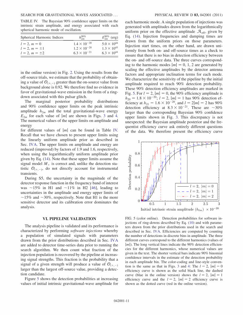
Figure 5 shows the detection probabilities at increasingvalues of initial intrinsic gravitational-wave amplitude for

each harmonic mode. A single population of injections wasgenerated with amplitudes drawn from the logarithmicallyuniform prior on the effective amplitude Aeff , given byEq. (14). Injection frequencies and damping times aredrawn from the uniform priors on those parameters.Injection start times, on the other hand, are drawn uni-formly from both on- and off-source times as a check toensure that there is no bias in detection efficiency betweenthe on- and off-source data. The three curves correspond-ing to the harmonic modes jmj ¼ 0, 1, 2 are generated byscaling the effective amplitudes by the detector antennafactors and appropriate inclination terms for each mode.We characterize the sensitivity of the pipeline by the initialamplitude required to reach 90% detection probability.These 90% detection efficiency amplitudes are marked inFig. 5. For l ¼ 2, jmj ¼ 0, the 90% efficiency amplitude ish20 ¼ 1:8� 10�20; l ¼ 2, jmj ¼ 1 has 90% detection ef-ficiency at h21 ¼ 1:6� 10�20, and l ¼ 2jmj ¼ 2 has 90%detection efficiency at 8:3� 10�21. These are �30%larger than the corresponding Bayesian 90% confidenceupper limits shown in Fig. 3. This discrepancy is notunexpected: the Bayesian amplitude posterior and the fre-quentist efficiency curve ask entirely different questionsof the data. We therefore present the efficiency curve

TABLE IV. The Bayesian 90% confidence upper limits on theintrinsic strain amplitude, and energy associated with eachspherical harmonic mode of oscillation.

Spherical Harmonic Indices h90%2m E90%2m (erg)

l ¼ 2, m ¼ 0 1:4� 10�20 5:0� 1044

l ¼ 2, m ¼ �1 1:2� 10�20 1:3� 1045

l ¼ 2, m ¼ �2 6:3� 10�21 6:3� 1044

FIG. 5 (color online). Detection probabilities for software in-jections of ring-downs described by Eq. (10) and with parame-ters drawn from the prior distributions used in the search anddescribed in Sec. IVA. Efficiencies are computed by countingthe number of detections in discrete bins in amplitude. The threedifferent curves correspond to the different harmonics (values ofjmj). The long vertical lines indicate the 90% detection efficien-cies for the different harmonics, whose numerical values aregiven in the text. The shorter vertical bars indicate 90% binomialconfidence intervals in the estimate of the detection probabilityin each amplitude bin. The color-coding and line-style conven-tion is the same as that in Figs. 3 and 4: The l ¼ 2, jmj ¼ 0efficiency curve is shown as the solid black line, the dashedcurve (blue in the online version) shows the l ¼ 2, jmj ¼ 1efficiency curve and the l ¼ 2, jmj ¼ 2 efficiency curve isshown as the dotted curve (red in the online version).

SEARCH FOR GRAVITATIONAL WAVES ASSOCIATED . . . PHYSICAL REVIEW D 83, 042001 (2011)

042001-11

purely as evidence that the analysis pipeline could havedetected a putative gravitational-wave signal, if there wasone present. The Bayesian upper limits, on the other hand,represent the strength of a gravitational-wave signal webelieve could have been present, given the on-sourceobservations.

VII. DISCUSSION

We have performed a search for gravitational-waveemission associated with a timing glitch in PSR B0833-45, the Vela pulsar, during the fifth LIGO science run.This search targeted ring-down signals in the frequencyrange [1, 3] kHz, with damping times in the range[50, 500] ms. No gravitational-wave detection candidatewas found. We place Bayesian 90% confidence upperlimits on the intrinsic peak gravitational-wave amplitudeand total gravitational-wave energy emitted by each quad-rupolar spherical harmonic mode, assuming that only asingle mode dominates any neutron star oscillations asso-ciated with the glitch. The amplitude and energy upperlimits for the different modes are reported in Table IV.The upper limits for each value of jmj agree with oneanother to within a factor of �2. Investigations of theimpact of calibration uncertainties under a variety of sce-narios suggest that the uncertainties in these upper limitsare no more than �15% and �30% in amplitude andenergy, respectively.

Having presented upper limits on the gravitational-waveemission for the different possible values of the indexm, wemay ask what the physical interest is in the different cases.In the absence of a definitive model of the glitch mecha-nism, it is not possible to say in advance which m value islikely to be dominant. However, the different symmetriescorresponding to the different m values offers some insightinto the possible glitch mechanism. The jmj ¼ 0 case cor-responds to the excitation of modes whose eigenfunctionsare symmetric about the rotation axis. In the context ofglitches, this would be rather natural, as glitches are thoughtto be caused either by the buildup of a rotational lag (as inthe superfluid model) or by a buildup of elastic strainenergy in response to a decreasing centrifugal force (thestar-quake model); both of these are axisymmetric in na-ture. The jmj ¼ 1 case might correspond to a glitch thatbegins at one point in the star before propagating outwards.The jmj ¼ 2 case might correspond to a glitch that inheritsthe symmetry of the magnetic dipole field that is believed topower the bulk of the star’s spin-down and radio pulsaremission. Clearly, a gravitational-wave observation indicat-ing which value of m (if any) of these is dominant willprovide a unique insight into the glitch mechanism.

It is natural to compare the upper limits presented herewith other gravitational wave searches for f-mode ring-downs. The only other search for a single f-mode event[13] presents a best upper limit of E90%

GW ¼ 2:4� 1048 ergon the energy emitted in gravitational waves via f-mode

induced ring-down signals associated with a flarefrom SGR 1806-20 on UTC 2006-08-24 14:55:26. In thatanalysis, however, the upper limits assume isotropicgravitational-wave emission. In addition, the nominal dis-tance of SGR 1806-20 is 10 kpc. To compare our resultswith those in [13], we must rescale our upper limit on theeffective amplitude Aeff to a source distance of 10 kpc,assume isotropic gravitational-wave emission and use the

average antenna factor of ðF2þ þ F2�Þ1=2 ¼ 0:3. We thenfind our equivalent, isotropic energy upper limit to be1:3� 1048 erg, a factor of �2 lower than that in [13].This improvement is to be expected since the analysispresented here assumes that the signal waveform is adecaying sinusoid. The analysis in [13], by contrast, doesnot rely on a particular waveform and is designed to searchfor bursts of excess power with durations and frequenciescompatible with f-mode ring-down signals.Following the arguments laid out in Sec. III, the char-

acteristic energy of a pulsar glitch is believed to be of order1038 or 1042 erg, depending on the mechanism. Our currentenergy upper limits are 2–3 orders of magnitude above(weaker than) the more optimistic theoretical limit. Thenext generation of gravitational-wave observatories cur-rently under construction, such as advanced LIGO [47]and advanced Virgo [48], is expected to have noise ampli-tude more than an order of magnitude lower than in thecurrent LIGO detectors at f-mode frequencies. This cor-responds to probing energies more than 2 orders of magni-tude lower than is currently possible, comparable to theorder 1042 erg of the most optimistic theoretical predic-tions. The detection of gravitational waves associated witha Vela glitch in the advanced interferometer era is thereforepossible and would provide compelling observationalevidence for the star-quake theory of pulsar glitches.According to current conceptual design [49], the plannedEinstein Telescope would improve noise amplitude atf-mode frequencies another order of magnitude beyondadvanced LIGO, thereby improving the Vela glitch energysensitivity 2 orders of magnitude to of order 1040 erg.

ACKNOWLEDGMENTS

The authors gratefully acknowledge the support of theUnited States National Science Foundation for the con-struction and operation of the LIGO Laboratory and theScience and Technology Facilities Council of the UnitedKingdom, the Max-Planck-Society, and the State ofNiedersachsen/Germany for support of the constructionand operation of the GEO600 detector. The authors alsogratefully acknowledge the support of the research bythese agencies and by the Australian Research Council,the Council of Scientific and Industrial Research ofIndia, the Istituto Nazionale di Fisica Nucleare of Italy,the Spanish Ministerio de Educacion y Ciencia,the Conselleria d’Economia Hisenda i Innovacio of theGovern de les Illes Balears, the Royal Society, the

J. ABADIE et al. PHYSICAL REVIEW D 83, 042001 (2011)

042001-12

Scottish Funding Council, the Scottish UniversitiesPhysics Alliance, The National Aeronautics and SpaceAdministration, the Carnegie Trust, the LeverhulmeTrust, the David and Lucile Packard Foundation, the

Research Corporation, and the Alfred P. SloanFoundation. This paper has been assigned LIGODocument No. P1000030-v11.

[1] B. P. Abbott et al., Astrophys. J. 713, 671 (2010).[2] J. Abadie et al. (LIGO Scientific Collaboration, Virgo

Collaboration), Phys. Rev. D 82, 102001 (2010).[3] J. Abadie et al., Astrophys. J. 715, 1453 (2010).[4] K. S. Thorne and A. Campolattaro, Astrophys. J. 149, 591

(1967).[5] R. Price and K. S. Thorne, Astrophys. J. 155, 163 (1969).[6] K. S. Thorne, Astrophys. J. 158, 1 (1969).[7] K. S. Thorne, Astrophys. J. 158, 997 (1969).[8] A. Campolattaro and K. S. Thorne, Astrophys. J. 159, 847

(1970).[9] J. R. Ipser and K. S. Thorne, Astrophys. J. 181, 181 (1973).[10] K. D. Kokkotas and B. Schmidt, Living Rev. Relativity 2

(1999) [http://relativity.livingreviews.org/Articles/lrr-1999-2/].

[11] M. Benacquista, D.M. Sedrakian, M.V. Hairapetyan,K.M. Shahabasyan, and A.A. Sadoyan, Astrophys. J.Lett. 596, L223 (2003).

[12] J. A. de Freitas Pacheco, Astronomical and AstrophysicalTransactions 336, 397 (1998) [http://aa.springer.de/bibs/8336001/2300397/small.htm].

[13] B. P. Abbott et al., Phys. Rev. Lett. 101, 211102 (2008).[14] B. P. Abbott et al., Astrophys. J. Lett. 701, L68 (2009).[15] R. Oechslin and H. Janka, Phys. Rev. Lett. 99, 121102

(2007).[16] J. Middleditch, F. E. Marshall, Q.D. Wang, E. V. Gotthelf,

and W. Zhang, Astrophys. J. 652, 1531 (2006).[17] P.W. Anderson and N. Itoh, Nature (London) 256, 25

(1975).[18] S. Buchner and C. Flanagan, in 40 Years of Pulsars:

Millisecond Pulsars, Magnetars and More, AIP Conf.Proc. No. 983 (AIP, New York, 2008), pp. 145–147.

[19] S. L. Shemar and A.G. Lyne, Mon. Not. R. Astron. Soc.282, 677 (1996) [http://adsabs.harvard.edu/abs/1996MNRAS.282..677S].

[20] G. B. Hobbs, R. T. Edwards, and R.N. Manchester, Mon.Not. R. Astron. Soc. 369, 655 (2006).

[21] C. S. Flanagan and S. J. Buchner, Central BureauElectronic Telegrams 595, 1 (2006) [http://www.cfa.harvard.edu/iau/cbet/000500/CBET000595.txt].

[22] R. G. Dodson, P.M. McCulloch, and D. R. Lewis,Astrophys. J. Lett. 564, L85 (2002).

[23] C. Y. Ng and R.W. Romani, Astrophys. J. 673, 411 (2008).[24] R. Dodson, D. Legge, J. E. Reynolds, and P.M.

McCulloch, Astrophys. J. 596, 1137 (2003).

[25] Australia Telescope National Facility Pulsar Cataloguehttp://www.atnf.csiro.au/research/pulsar/psrcat.

[26] R. N. Manchester, G. B. Hobbs, A. Teoh, and M. Hobbs,Astron. J. 129, 1993 (2005).

[27] B. P. Abbott et al., Rep. Prog. Phys. 72, 076901 (2009).[28] N. Andersson, G. L. Comer, and R. Prix, Mon. Not. R.

Astron. Soc. 354, 101 (2004).[29] A. Melatos, C. Peralta, and J. S. B. Wyithe, Astrophys. J.

672, 1103 (2008).[30] T. Sidery, A. Passamonti, and N. Andersson, Mon. Not. R.

Astron. Soc. 405, 1061 (2010) [http://onlinelibrary.wiley.com/doi/10.1111/j.1365-2966.2010.16497.x/abstract].

[31] C. A. van Eysden and A. Melatos, Classical QuantumGravity 25, 225020 (2008).

[32] M. Ruderman, Nature (London) 223, 597 (1969).[33] G. Baym and D. Pines, Ann. Phys. (N.Y.) 66, 816 (1971).[34] K. S. Thorne, Rev. Mod. Phys. 52, 299 (1980).[35] N. Andersson and K.D. Kokkotas, Mon. Not. R. Astron.

Soc. 299, 1059 (1998).[36] O. Benhar, V. Ferrari, and L. Gualtieri, AIP Conf. Proc.

751, 211 (2005).[37] J.M. Lattimer and M. Prakash, Astrophys. J. 550, 426

(2001).[38] A. G. Lyne, S. L. Shemar, and F.G. Smith, Mon. Not. R.

Astron. Soc. 315, 534 (2000).[39] J. Clark, I. S. Heng, M. Pitkin, and G. Woan, Phys. Rev. D

76, 043003 (2007).[40] J. Veitch and A. Vecchio, Classical Quantum Gravity 25,

184010 (2008).[41] A. C. Searle, P. J. Sutton, M. Tinto, and G. Woan, Classical

Quantum Gravity 25, 114038 (2008).[42] P. Jaranowski, A. Krolak, and B. F. Schutz, Phys. Rev. D

58, 063001 (1998).[43] C. Y. Ng and R.W. Romani, Astrophys. J. 601, 479

(2004).[44] B. P. Abbott et al., Phys. Rev. D 80, 102002 (2009).[45] J. Veitch and A. Vecchio, Phys. Rev. D 81, 062003

(2010).[46] J. Abadie et al. (LIGO Scientific Collaboration, Nucl.

Instrum. Methods Phys. Res., Sect. A 624, 223 (2010).[47] G.M. Harry et al., Classical Quantum Gravity 27, 084006

(2010).[48] http://wwwcascina.virgo.infn.it/advirgo/.[49] M. Punturo et al., Classical Quantum Gravity 27, 084007

(2010).

SEARCH FOR GRAVITATIONAL WAVES ASSOCIATED . . . PHYSICAL REVIEW D 83, 042001 (2011)

042001-13