gravitational waves · pdf fileefficient analysis algorithms for gravitational waves and...
TRANSCRIPT

Efficient analysis algorithms for
Gravitational Wavesand
CosmologyO T:
Gravitational Waves from Inspiraling Binaries and Cosmological Ramifications
BSanjit Mitra
A T F D
Doctor of Philosophy( in Physics )
University of Pune
S: Prof. Sanjeev DhurandharC-: Prof. Tarun Souradeep
Inter-University Centre for Astronomy and AstrophysicsPost Bag 4, Ganeshkhind, Pune 411 007, INDIA
DECEMBER 2006


Dedicated to Nature
of which I am a part

iv

v
Contents
Dedication iii
Acknowledgment xiii
List of Publications xv
Declaration xvii
Abstract xix
1 Introduction 1
1.1 Basics . . . . . . . . . . . . . . . . . . . . . . . . . . . . . . . . . . . . . 1
1.1.1 Gravitational Waves (GW) . . . . . . . . . . . . . . . . . . . . . 1
1.1.2 Cosmic Microwave Background (CMB) . . . . . . . . . . . . . 2
1.2 Search for GW from Inspiraling Binaries: Chebyshev Interpolation . 3
1.3 Search for GW Background: Radiometer Analysis . . . . . . . . . . . 5
1.4 Deconvolution of Sky-Maps . . . . . . . . . . . . . . . . . . . . . . . . 5
1.5 Non-circular Beam Correction to CMB Power Spectrum . . . . . . . . 6
1.6 Organization of the Thesis . . . . . . . . . . . . . . . . . . . . . . . . . 7
2 Introduction to Gravitational Waves (GW) 9
2.1 Gravitational Waves . . . . . . . . . . . . . . . . . . . . . . . . . . . . 10
2.1.1 General Relativity: Einstein’s Equation . . . . . . . . . . . . . 10
2.1.2 Weak field limit: Linearized Theory . . . . . . . . . . . . . . . 10
2.1.3 Plane Polarized Monochromatic Gravitational Waves . . . . . 14
2.2 Detection . . . . . . . . . . . . . . . . . . . . . . . . . . . . . . . . . . . 14
2.3 Sources and Analysis Strategies . . . . . . . . . . . . . . . . . . . . . . 18
2.4 Summary and Conclusion . . . . . . . . . . . . . . . . . . . . . . . . . 20

vi CONTENTS
3 Search for GW from Inspiraling Binaries: Chebyshev Interpolation 21
3.1 Chirp Signal . . . . . . . . . . . . . . . . . . . . . . . . . . . . . . . . . 23
3.2 Dense Search . . . . . . . . . . . . . . . . . . . . . . . . . . . . . . . . . 25
3.2.1 Matched Filtering . . . . . . . . . . . . . . . . . . . . . . . . . . 25
3.2.2 Template placement . . . . . . . . . . . . . . . . . . . . . . . . 26
3.2.3 Choice of parameter . . . . . . . . . . . . . . . . . . . . . . . . 29
3.3 Efficient Search Algorithms . . . . . . . . . . . . . . . . . . . . . . . . 30
3.4 Interpolated Search . . . . . . . . . . . . . . . . . . . . . . . . . . . . . 32
3.4.1 Interpolation of the Wiener filter output . . . . . . . . . . . . . 32
3.4.2 Search strategy . . . . . . . . . . . . . . . . . . . . . . . . . . . 36
3.4.3 Template placement . . . . . . . . . . . . . . . . . . . . . . . . 38
3.5 Comparison between Dense and Interpolated search: ROC curves . . 42
3.6 Summary and Conclusion . . . . . . . . . . . . . . . . . . . . . . . . . 44
4 Search for GW Background (GWB): Radiometer Analysis 49
4.1 Stochastic Gravitational Wave Background (GWB) . . . . . . . . . . . 50
4.2 Sources of GWB . . . . . . . . . . . . . . . . . . . . . . . . . . . . . . . 54
4.3 Detection of GWB: Radiometer Analysis . . . . . . . . . . . . . . . . . 56
4.3.1 Cross-correlation statistic . . . . . . . . . . . . . . . . . . . . . 57
4.3.2 Correlation between GW Strains . . . . . . . . . . . . . . . . . 62
4.3.3 Detector Noise . . . . . . . . . . . . . . . . . . . . . . . . . . . 64
4.3.4 Optimal Filter . . . . . . . . . . . . . . . . . . . . . . . . . . . . 65
4.3.5 Observed Point Estimate and SNR . . . . . . . . . . . . . . . . 69
4.3.6 Summary . . . . . . . . . . . . . . . . . . . . . . . . . . . . . . 71
4.4 Applications . . . . . . . . . . . . . . . . . . . . . . . . . . . . . . . . . 73
4.4.1 All-sky isotropic background . . . . . . . . . . . . . . . . . . . 74
4.4.2 Directed Search . . . . . . . . . . . . . . . . . . . . . . . . . . . 76
4.5 Summary and Conclusion . . . . . . . . . . . . . . . . . . . . . . . . . 79
5 Introduction to the Cosmic Microwave Background (CMB) 81
5.1 Origin . . . . . . . . . . . . . . . . . . . . . . . . . . . . . . . . . . . . . 82
5.2 CMB Anisotropy . . . . . . . . . . . . . . . . . . . . . . . . . . . . . . 84
5.3 Angular Power Spectrum: Cosmic Variance . . . . . . . . . . . . . . . 86
5.4 Experiments . . . . . . . . . . . . . . . . . . . . . . . . . . . . . . . . . 89
5.5 Summary and Conclusion . . . . . . . . . . . . . . . . . . . . . . . . . 90
CONTENTS vii
6 Beams and Deconvolution in CMB and GWB Mapmaking: Analysis and For-malism 91
6.1 Beam Function . . . . . . . . . . . . . . . . . . . . . . . . . . . . . . . . 92
6.2 Observed CMB Data . . . . . . . . . . . . . . . . . . . . . . . . . . . . 92
6.3 Observed (Directed) GW Radiometer Point Estimate . . . . . . . . . . 95
6.4 Maximum Likelihood (ML) skymap Estimation . . . . . . . . . . . . . 101
6.5 ML Estimation of CMB Anisotropy Map . . . . . . . . . . . . . . . . . 103
6.6 ML Estimation of GWB Anisotropy . . . . . . . . . . . . . . . . . . . . 104
6.6.1 Basic Analysis of Skymap . . . . . . . . . . . . . . . . . . . . . 104
6.6.2 Extensions of the simple MapMaking . . . . . . . . . . . . . . 105
6.6.3 Multipole moments from the directed search . . . . . . . . . . 107
6.6.4 Multipole moments from isotropic all-sky search . . . . . . . . 108
6.7 Summary and Conclusions . . . . . . . . . . . . . . . . . . . . . . . . 111
7 Numerical Implementation of ML Mapmaking for GWB 113
7.1 Preparation of Simulated Data . . . . . . . . . . . . . . . . . . . . . . . 114
7.2 Preparation of the “Dirty” Maps . . . . . . . . . . . . . . . . . . . . . 116
7.3 Computation of the Beam Matrix . . . . . . . . . . . . . . . . . . . . . 117
7.4 Deconvolution: The “Clean” Maps . . . . . . . . . . . . . . . . . . . . 120
7.5 Results and Comparisons . . . . . . . . . . . . . . . . . . . . . . . . . 123
7.6 Summary and Conclusion . . . . . . . . . . . . . . . . . . . . . . . . . 125
8 Non-circular Beam Correction to CMB Power Spectrum:Perturbative Analysis 127
8.1 Pseudo-Cl Approach to Non-circular Beam Correction . . . . . . . . . 128
8.2 Window functions of CMB experiments: a brief primer . . . . . . . . 131
8.2.1 Window function for circular beams . . . . . . . . . . . . . . . 133
8.2.2 Window function for non-circular beams . . . . . . . . . . . . 134
8.3 Bias Matrix . . . . . . . . . . . . . . . . . . . . . . . . . . . . . . . . . 138
8.3.1 Circular Symmetric Beam . . . . . . . . . . . . . . . . . . . . . 140
8.3.2 Non-circular Beam . . . . . . . . . . . . . . . . . . . . . . . . . 141
8.4 Error-Covariance Matrix . . . . . . . . . . . . . . . . . . . . . . . . . . 148
8.4.1 Circular Beam . . . . . . . . . . . . . . . . . . . . . . . . . . . . 151
8.4.2 Non-circular Beam . . . . . . . . . . . . . . . . . . . . . . . . . 151
8.5 Discussion and Conclusion . . . . . . . . . . . . . . . . . . . . . . . . 155

viii CONTENTS
9 Non-circular Beam Correction to CMB Power Spectrum:Complete Analysis Framework 1599.1 Analytical Framework . . . . . . . . . . . . . . . . . . . . . . . . . . . 160
9.1.1 Bias in the pseudo-Cl estimator . . . . . . . . . . . . . . . . . . 1609.1.2 Evaluation of the Bias Matrix . . . . . . . . . . . . . . . . . . . 1629.1.3 Checking different limits . . . . . . . . . . . . . . . . . . . . . . 166
9.2 Implementation . . . . . . . . . . . . . . . . . . . . . . . . . . . . . . . 1679.3 Discussions and Conclusion . . . . . . . . . . . . . . . . . . . . . . . . 171
10 Conclusion 173
A Properties of the Chebyshev Polynomials 177
B Directed GW Radiometer Beam: Stationary Phase Approximation 179B.1 Beam Pattern: SPA Trajectory . . . . . . . . . . . . . . . . . . . . . . . 180
B.1.1 The case of small ∆Ω . . . . . . . . . . . . . . . . . . . . . . . . 181B.1.2 General SPA solution . . . . . . . . . . . . . . . . . . . . . . . . 183
B.2 Evaluation of the Beam Function on SPA trajectory . . . . . . . . . . . 184
C Cosmic Variance 187
D Elliptical Gaussian fit to the WMAP beam maps 189
E Derivations for perturbative analysis of beam correction to pseudo-Cl es-timator 195
F Derivations for general analysis of beam correction to pseudo-Cl estimator201F.1 Useful formulae . . . . . . . . . . . . . . . . . . . . . . . . . . . . . . . 201F.2 Expansion of Wigner-D Function . . . . . . . . . . . . . . . . . . . . . 202F.3 Evaluation of Jll′′l′
nm′′mm′ using sinusoidal expansion of Wigner-d . . . . 205F.4 Evaluation of Jll′′l′
nm′′mm′ using Clebsch-Gordon series and sinusoidalexpansion of Wigner-d . . . . . . . . . . . . . . . . . . . . . . . . . . . 207
F.5 The full sky and circular beam limit . . . . . . . . . . . . . . . . . . . 209F.6 The circular beam limit with cut sky . . . . . . . . . . . . . . . . . . . 211F.7 The full sky limit with non-circular beam . . . . . . . . . . . . . . . . 213
G Fast computation of non-circular beam correction to CMB power spectrum215

ix
List of Tables
3.1 Comparison between dense and interpolated search . . . . . . . . . . 44
8.1 Definition of parameters that quantify non-circularity . . . . . . . . . 138
B.1 Coordinate of the LIGO detectors . . . . . . . . . . . . . . . . . . . . . 182
D.1 Ellipticities of WMAP beams . . . . . . . . . . . . . . . . . . . . . . . 193

x LIST OF TABLES
xi
List of Figures
2.1 Effect of GW on matter: Detection scheme . . . . . . . . . . . . . . . . 15
2.2 GW Detectors . . . . . . . . . . . . . . . . . . . . . . . . . . . . . . . . 16
2.3 LIGO-I sensitivity curves . . . . . . . . . . . . . . . . . . . . . . . . . . 17
3.1 Illustration of Matched Filtering . . . . . . . . . . . . . . . . . . . . . . 27
3.2 Ambiguity function . . . . . . . . . . . . . . . . . . . . . . . . . . . . . 30
3.3 Illustration of Interpolated Search . . . . . . . . . . . . . . . . . . . . . 37
3.4 Variation of bias with no. of interpolated search templates . . . . . . 40
3.5 Variation of Match with signal location . . . . . . . . . . . . . . . . . . 41
3.6 Comparison: False Alarm & False Dismissal probability . . . . . . . . 45
3.7 Comparison: ROC Curves . . . . . . . . . . . . . . . . . . . . . . . . . 46
4.1 Inflationary GWB spectra and detectability using the advanced LIGOdetectors . . . . . . . . . . . . . . . . . . . . . . . . . . . . . . . . . . . 55
4.2 GWB spectra and detectability landscape . . . . . . . . . . . . . . . . 56
4.3 Time independent overlap reduction function . . . . . . . . . . . . . . 75
4.4 Geometry of an elementary radiometer . . . . . . . . . . . . . . . . . 77
4.5 A test sky map made using the GWB radiometer . . . . . . . . . . . . 78
5.1 Evolution of anisotropies in the universe . . . . . . . . . . . . . . . . 83
5.2 Observed CMB frequency spectrum by COBE FIRAS . . . . . . . . . 84
5.3 WMAP CMB anisotropy sky . . . . . . . . . . . . . . . . . . . . . . . . 85
5.4 Observed CMB Power Spectrum . . . . . . . . . . . . . . . . . . . . . 88
5.5 CMB Experiments . . . . . . . . . . . . . . . . . . . . . . . . . . . . . . 89
6.1 WMAP image planes . . . . . . . . . . . . . . . . . . . . . . . . . . . . 94
6.2 Numerical and Theoretical GW radiometer beam patterns . . . . . . 97
6.3 Contour plots of GW radiometer beam patterns . . . . . . . . . . . . 98

xii LIST OF FIGURES
7.1 A typical GW radiometer Beam Matrix . . . . . . . . . . . . . . . . . . 1207.2 Deconvolved (simulated) GWB skymaps . . . . . . . . . . . . . . . . 126
8.1 Illustration of beam rotation . . . . . . . . . . . . . . . . . . . . . . . . 1348.2 WMAP Q1 Beam . . . . . . . . . . . . . . . . . . . . . . . . . . . . . . 1358.3 Bias matrix without beam rotation . . . . . . . . . . . . . . . . . . . . 1458.4 Characteristics of the bias matrix elements (no beam rotation) . . . . 1468.5 Effect of beam rotation on bias matrix . . . . . . . . . . . . . . . . . . 1478.6 Cl estimation error due to non-circular beams . . . . . . . . . . . . . . 1498.7 Cl estimation error published in the WMAP 3yr results [96] . . . . . . 1508.8 Covariance of Cl’s due to beam non-circularity . . . . . . . . . . . . . 154
9.1 The original Kp2 mask . . . . . . . . . . . . . . . . . . . . . . . . . . . 1709.2 Comparison of mask transforms . . . . . . . . . . . . . . . . . . . . . 170
A.1 Plots of the first few orders of Chebyshev polynomials . . . . . . . . 178
B.1 Cone traced out by a radiometer baseline . . . . . . . . . . . . . . . . 180B.2 Beam functions in flat latitude-longitude grid . . . . . . . . . . . . . . 181
D.1 Profile of WMAP Q-beam fitted using IRAF . . . . . . . . . . . . . . . 190D.2 IRAF estimated parameters characterizing WMAP beams . . . . . . . 191

xiii
Acknowledgment
Over the past five years, the research I have carried out would not have beenpossible without the help of people from IUCAA, the LIGO Scientific Collaboration(LSC) and many others from scientific and nonscientific communities. This thesisis too short to acknowledge all of them, still, I would not miss this opportunity tothank few of the special ones.
I whole heartedly thank my supervisors Prof. Sanjeev Dhurandhar and Prof.Tarun Souradeep for offering me the opportunity to work with them. The careand guidance they have provided me during my Ph.D. has played a crucial role toshape my career as a researcher. I am deeply obliged to Dr. Albert Lazzarini forhis support and encouragement during my visit to Caltech. It would not have beenpossible to finish the thesis in time without his constant supervision. I would thankProf. Lee Samuel Finn, Dr. Vuk Mandic, Dr. Sukanta Bose, the stochastic group ofthe LSC and the other members of the LSC for being my collaborators.
My academic work and social activities were greatly benefitted by the help thatI got from Prof. J. V. Narlikar, Prof. N. K. Dadhich, Prof. T. Padmanabhan, Prof. A.K. Kembhavi, Prof. S. Tandon, Prof. V. Sahni, Dr. R. Misra, Dr. S. Ravindranath, Dr.S. Engineer, Dr. V. Chellathurai, Ms. S. Ponrathnam, Ms. N. Bawdekar and everyother member of IUCAA. I also remember all my past teachers on this occasion,who have equally supported me in the respective stages of my life.
During my stay at IUCAA, it has been a pleasure to be in the constant com-pany of IUCAAns, specially Anand0-da, Atul, Rita, Samir, Subharthi-da, Arnab-da,Sudipta, Somu, Susmita, Nirupam, Gauranga, Minu, Arman, Ghazal, Abhishek,Tirtho-da, Sushan-di, Tapan, Himan, Amir, Hum Chand for every little thing. Be-yond the world of IUCAA, I fondly remember Rasiya, Aditya, Tapu, Debjani, Manoj,Shweta, Anindya, Rajarshi and all my friends in Kolkata, where my home is.
Finally and very importantly, I could not have gone anywhere in life but for theconstant presence of my parents, uncle, brother, Shamin and all the family members.

xiv ACKNOWLEDGMENT

xv
List of Publications
1. T. Souradeep, S. Mitra, A. S. Sengupta, S. Ray, and R. Saha, “CMB powerspectrum estimation with the non-circular beam”, in Proceedings of the “Fun-damental Physics With CMB workshop” March 23-25, 2006, New Astron. Rev.,vol. 50, p. 1030. 2006. astro-ph/0608505.
2. S. Mitra, S. V. Dhurandhar, and L. S. Finn, “Improving the efficiency of thedetection of gravitational wave signals from inspiraling compact binaries:Chebyshev interpolation”, Phys. Rev. D72 (2005) 102001, gr-qc/0507011.
3. S. Mitra, A. S. Sengupta, and T. Souradeep, “CMB power spectrum estimationusing noncircular beams”, Phys. Rev. D70 (2004) 103002, astro-ph/0405406.
4. S. Mitra, S. Dhurandhar, T. Souradeep, A. Lazzarini, V. Mandic, and S. Bose,“Gravitational wave radiometry: Deconvolution of the GWB sky map”. Inpreparation, 2006.
5. S. Mitra, A. S. Sengupta, S. Ray, R. Saha, and T. Souradeep, “CMB powerspectrum estimation with the non-circular beam”. In preparation, 2006.
6. LIGO Scientific Collaboration, B. Abbott et al., “Searching for a stochasticbackground of gravitational waves with LIGO”, astro-ph/0608606.
7. LIGO Scientific Collaboration, B. Abbott et al., “Coherent searches for periodicgravitational waves from unknown isolated sources and scorpius x-1: resultsfrom the second LIGO science run”, gr-qc/0605028.
8. LIGO Scientific Collaboration, B. Abbott et al., “Joint LIGO and tama300search for gravitational waves from inspiralling neutron star binaries”, Phys.Rev. D73 (2006) gr-qc/0512078.

xvi LIST OF PUBLICATIONS
9. LIGO Scientific Collaboration, B. Abbott et al., “Search for gravitational wavebursts in LIGO’s third science run”, Class. Quant. Grav. 23 (2006) S29,gr-qc/0511146.
10. LIGO Scientific Collaboration, B. Abbott et al., “Search for gravitational wavesfrom binary black hole inspirals in LIGO data”, Phys. Rev. D73 (2006) 062001,gr-qc/0509129.
11. LIGO Scientific Collaboration, B. Abbott et al., “First all-sky upper limitsfrom LIGO on the strength of periodic gravitational waves using the houghtransform”, Phys. Rev. D72 (2005) 102004, gr-qc/0508065.
12. LIGO Scientific Collaboration, B. Abbott et al., “Upper limits on a stochas-tic background of gravitational waves”, Phys. Rev. Lett. 95 (2005) 221101,astro-ph/0507254.
13. T. K. Das, J. K. Pendharkar, and S. Mitra, “Multitransonic black hole accre-tion disks with isothermal standing shocks”, Astrophys. J. 592 (2003) 1078,astro-ph/0301189.

DECLARATION xvii
Certificate of the Guides
CERTIFIED that the work incorporated in the thesis “Gravitational Wavesfrom Inspiraling Binaries and Cosmological Ramifications” submitted by Mr. San-jit Mitra was carried out by the candidate under our supervision/ guidance. Suchmaterial as has been obtained from other sources has been duly acknowledged inthe thesis.
Prof. Sanjeev Dhurandhar Prof. Tarun Souradeep(Thesis Supervisor) (Thesis Co-supervisor)
Declaration by the Candidate
I declare that the thesis entitled “Gravitational Waves from Inspiraling Binariesand Cosmological Ramifications” submitted by me for the degree of Doctor ofPhilosophy is the record of work carried out by me during the period from Decem-ber 2003 to December 2006 under the guidance of Prof. Sanjeev Dhurandhar &Prof. Tarun Souradeep and has not formed the basis for the award of any degree,diploma, associateship, fellowship, titles in this or any other University or otherinstitution of Higher learning.
I further declare that the material obtained from other sources has been dulyacknowledged in the thesis.
Date:Place: Sanjit Mitra

xviii

xix
Abstract
The past five years have ushered in a new era of observational astronomy. Groundbased gravitational wave (GW) detectors - LIGO, TAMA and GEO - have startedtaking science quality data. Space based cosmic microwave background (CMB) ex-periments - WMAP - has produced a true image of the CMB temperature anisotropysky and also has mapped the CMB polarization sky. Efficiently extracting maxi-mum amount of science out of these data rich experiments pose challenges to themodern analysis techniques. Few of the issues regarding efficient analysis of datahave been addressed in my thesis.
Detection of GW from inspiraling binaries is perhaps the most important ex-perimental goal in experimental general relativity for the next few years. However,extracting the true GW strain signal from much stronger random detector noise isquite challenging. Current analysis strategy relies on matched filtering techniqueswhich is computationally expensive. We have developed an interpolation schemefor efficient implementation of matched filtering based analysis algorithms. We usenumerical simulations to show that this new method reduces computational cost,thereby increasing the volume the parameter space that can be searched with theavailable computing resources.
Measurement of the anisotropy of the CMB and the gravitational wave back-ground (GWB) are equally important challenges in experimental cosmology toprobe the history of the early universe. Usually the imaged skymaps are con-volved with the instrumental beam functions - also known as the point spreadfunctions (PSF). Unbiased estimation of the anisotropies of these backgrounds re-quires development of smart analysis strategies. We have analytically formulatedand numerically implemented complete analysis frameworks to account for theeffects of beam functions in the analysis of CMB and GWB.
xx ABSTRACT
The thesis has been organized as follows:
• Chapter 1 provides an overall introduction and motivation on the workspresented in this thesis.
• Chapter 2 provides an introduction to Gravitational Waves (GW) and itssources, detectors and data analysis, essentially mentioning the features im-portant for the detection of GW.
• The Chebyshev interpolated search algorithm for efficient detection of GWfrom inspiraling binaries and the results are presented in Chapter 3.
• A brief introduction to stochastic Gravitational Wave Background (GWB) anda detailed review of the general radiometer analysis for the detection of GWBhas been presented in Chapter 4.
• Brief introduction to the theory and experiments of Cosmic Microwave Back-ground (CMB) and its anisotropy, emphasizing points which are relevant tothe work presented in this thesis, is provided in Chapter 5.
• The analytical formulation of beams and deconvolution in CMB and GWBanalysis is presented in Chapter 6.
• Implementation of radiometer deconvolution algorithm and application toGWB skymaps obtained from simulated detector outputs is presented inChapter 7.
• The leading order correction to CMB power spectrum due to non-circularbeams is estimated using a perturbative analysis in Chapter 8.
• General analysis framework for the pseudo-Cl approach to correct for non-circular beams including the effect of incomplete sky coverage is developedin Chapter 9.
• The summary of the main results obtained in this thesis and future directionsare mentioned in Chapter 10.

1
Chapter 1
Introduction
In the past few decades, astronomy, in particular, cosmology has emerged into aprecision science. A host of instruments have come up with advanced measure-ment techniques. These instruments produce large volumes of data and extractingmaximum amount of science out of these data is one of the primary goals of modernastronomy and astrophysics.
My thesis concerns with two very important areas of modern astronomy andcosmology - the analysis of data from gravitational wave and cosmic microwavebackground detectors. Though these detectors work differently, we shall see thatthe data analysis challenges posses many common attributes.
The overall introduction and motivation of this thesis is provided in this chap-ter. The discussions presented here will be brief; more detailed material can befound in the subsequent chapters.
1.1 Basics
1.1.1 Gravitational Waves (GW)
General theory of relativity (GR) has so far been the unchallenged theory of gravity.Unlike Newtonian theory of gravity, in GR, the effect of gravity does not affectinstantaneously - gravitational information travels at the speed of light and theinformation is carried by the gravitational waves. In the weak field approximation,GW can be considered as an external field over a background space-time - ripplesin space-time. GW are massless excitations, hence have two polarizations, + and ×.
GW interact weakly with matter, which makes them extremely difficult todetect. However, on a positive note, being weakly interacting with matter, GW can

2 Chapter 1. Introduction
travel large distances without getting absorbed or distorted. Detection of GW is,therefore, not only important to test GR, but promise a whole new possibility ofGW astronomy. When gravitational waves are incident on a local coordinate systemdefined by a set of test masses, the light travel time between two points changes.This principle is exploited for detecting GW. The GW strain is proportional to thedistance between particles, so long detectors are desired to improve the sensitivity.
Several detectors are under construction all over the world and proposed. Thedetectors are either bar detectors (ALLEGRO, EXPLORER, NAUTILUS) sensitiveto high (kHz) frequencies or interferometric detectors (LIGO, TAMA, GEO, VIRGO,LISA) at lower (mHz to few hundred Hz) frequencies. Since different sources havedifferent frequency spectrum, each detector is most sensitive to a specific class ofsources. The LIGO detectors, currently the most sensitive ones, TAMA and GEOhave started taking science quality data, which are being used to put upper limitson important astrophysical quantities. Besides terrestrial GW detectors, there areproposals to build interferometric space antennas.
GW are generated by massive bodies with varying moment of inertia. Thereare different sources of GW, with different frequency spectra. The sources have beenclassified into three major types depending on the time scales and characteristics:
1. Burst (inspiraling binaries, supernovae)
2. Stochastic (unmodeled sources, characterized by statistical expectations)
3. Continuous (pulsars)
The data analysis challenges and, therefore, strategies are different for each type ofsource. In this thesis we have considered an efficient strategy to extract the inspiralwaveform from a compact binary system (category 1). Secondly, we analyze andimplement targeted search for the stochastic GW background (category 2).
1.1.2 Cosmic Microwave Background (CMB)
The Big Bang theory is the currently accepted working model of the universe. Ac-cording the big bang model, the universe was a very hot plasma in its early stages.The photons were tightly coupled to the plasma in thermal equilibrium - attaininga black body distribution. As the universe expanded, the plasma recombined toneutral state where photons could then travel freely. This epoch of recombinationis known as the last scattering surface. Photons from the last scattering surface, re-ceived continuously from all directions, constitute the relic background. Due to the

1.2: Search for GW from Inspiraling Binaries: Chebyshev Interpolation 3
expansion of the universe, the photon density has decreased and due to cosmolog-ical redshift the wavelengths of the photons have increased. So the temperature ofthe background has decreased - currently at 2.7K, which corresponds to microwaveradiation. Thus the relic electro-magnetic radiation background of the hot earlyuniverse is called the cosmic microwave background (CMB).
The early universe was highly homogenous and isotropic. This fact is reflectedin the high degree of isotropy of CMB. However, the early universe also had smallinhomogeneities, which have grown to form the presently observed structures,like galaxies. These signatures are also present in CMB as µK fluctuations. CMBanisotropy is an extremely important probe of the early universe. Gaussian andstatistically isotropic CMB anisotropy can be completely characterized by its angularpower spectrum.
Since the first detection by COBE satellite of CMB anisotropy in 1992, a host ofterrestrial, balloon borne and space based experiments to measure CMB anisotropyhave been performed, commissioned and being proposed. The earth based exper-iments include interferometric detectors (e.g., CBI, DASI), scanning detectors (e.g.,ACBAR), balloon borne detectors (e.g., BOOMERang, Archeops) and the spacebased detectors include COBE and WMAP. Another spaced based mission, thePlanck surveyor, is planned in 2007. CMB observations have been used to pre-cisely constrain cosmological models and parameters. CMB research has taken theleading role in entering the era of precision cosmology. The precision of the exper-iments, however, demands unbiased analysis of data. Unbiased estimation of theCMB power spectrum by removing systematic effects is one of the broad concernsof this thesis.
1.2 Search for GW from Inspiraling Binaries: Chebyshev In-terpolation
GW interact weakly with matter, which makes them very difficult to detect. Thoughthe most advanced technologies of microscopic measurements are being used in thegravitational wave experiments, the detector outputs will be dominated by noise.However, the sources of gravitational waves, which are expected to be detectedwith the modern detectors, have been theoretically modeled. This knowledge canbe used to extract signal from noisy data. This is the only possible way of detectionof gravitational waves using the detectors which are currently operating or comingup in the near future.

4 Chapter 1. Introduction
If the phase of the expected signal is precisely modeled, matched filtering isoptimal. In the current analysis methodology, a theoretically modeled signal (tem-plate) is correlated with data for different sets of parameters that densely coverthe physically permitted parameter space and detection will be claimed if the cor-relation exceeds a pre-assigned threshold. The reason for such a dense coverageof parameter space is to minimize the chance that a real signal, near the detectionthreshold, will be missed by the parameter space sampling.
The current analysis is computationally expensive. Efforts are being made todevelop efficient search algorithms which would allow search over a larger volumeof parameter space with greater number of parameters. For small variations inthe parameters, the filter responses are strongly correlated, which is the case for adense search. This is the result of over sampling. The efficiency of search usingmatched filtering can be improved by optimally sampling the parameter space andthen reconstructing the likelihood (or the match) function. We have investigatedthe use of Chebyshev interpolation for reducing the number of templates that mustbe evaluated without sacrificing the efficiency of the search. Additionally, rather thanfocus on the “loss” of signal-to-noise associated with the finite number of filters inthe template bank, we evaluated the Receiver Operating Characteristic, or ROC, asa measure of the efficiency of a search technique. The ROC relates the false alarmprobability to the false dismissal probability of an analysis, which are the quantitiesthat bear most directly on the effectiveness of an analysis scheme.
The time-dependent signature of GW from compact inspiraling binaries is well-characterized function of a relatively small number of parameters, which makesthem very promising sources for the ground and space based interferometric de-tectors. As a demonstration we compared the present “dense sampling” analysismethodology with the “interpolation” methodology using Chebyshev polynomials,restricted to one dimension of the multi-dimensional analysis problem for inspi-raling binaries by plotting the ROC curves. We found that the interpolated searchcan be arranged to have the same false alarm and false dismissal probabilities asthe dense sampling strategy using 25% fewer templates. Generalized to the fullseven dimensional parameter space that characterizes the signal associated with aneccentric binary system of spinning neutron stars or black holes it suggests an orderof magnitude increase in computational efficiency. A reduction in the number oftemplates evaluations translates directly into an increase in the size of the parameterspace that can be analyzed and, thus, the science that can be accomplished with thedata.

1.3: Search for GW Background: Radiometer Analysis 5
1.3 Search for GW Background: Radiometer Analysis
The stochastic GW background arises from unresolved astrophysical sources andis predicted from the physics of the early universe. The measurement of the GWbackground (GWB) can probe the inhomogeneities of the nearby universe andimportant phenomena, like inflation, in the early universe.
By definition, stochastic signals are characterized by expectation values. Thebest strategy to detect GWB is to correlate the outputs of different detectors thathave independent noise. The correlation between noise streams will tend to cancelon time integration, but the common GW signal will add. This principle can be usedto measure the sky averaged strength of the GWB, as well as, to make a sky map.The sky map is made by introducing a phase shift between the detector outputs thataccounts for the delay between two detectors in receiving a signal from a certaindirection. Signals from a target direction is coherently added and signals from otherdirection tend to cancel out. This method is similar to the earth rotation imagesynthesis used in interferometric radio astronomy, hence we name this analysis asGW radiometer. Extending primary work on GW radiometry for special cases ofGWB, we have developed a general GW radiometer analysis strategy, which can beapplied to a broad range of GWB models.
1.4 Deconvolution of Sky-Maps
The observed sky maps of the GWB and CMB are both convolved with a beam (ora point spread function) - the image of a point source is not a point source, it is apattern of finite size. The estimation of the true skymap requires correction of theobserved “dirty” maps to eliminate the effects of the antenna pattern functions.
Unlike CMB experiments, the beam function of a GW radiometer has a highlyasymmetric pattern. The beam patterns also depend on the sky position. Ourfirst goal was to understand the beam pattern of the radiometer search. We usedstationary phase approximation (SPA) to analytically explain the beam patternswhich matched very well with the numerically obtained ones.
The next step was to remove the effect of beam function from the dirty maps.Several deconvolution algorithms exist in literature. Because of the broad similaritybetween the convolution equations of GWB and CMB, we followed a method thathas been successfully applied in CMB analysis - the maximum likelihood (ML)sky map estimation. We have developed the deconvolution algorithm for GWB

6 Chapter 1. Introduction
sky-maps based on the statistical and numerical methods suggested by the CMBanalysts. The method was numerically implemented and injected test maps wererecovered with a fairly good accuracy.
1.5 Non-circular Beam Correction to CMB Power Spectrum
The measurements of the angular power spectrum of the Cosmic Microwave Back-ground (CMB) anisotropy has proven crucial to the emergence of cosmology as aprecision science in recent years. In this remarkable data rich period, the limitationsto precision now arise from the the inability to account for finer systematic effectsin data analysis.
The optimal analysis to account for the effect of the beam function, a fullmaximum likelihood (ML) analysis, is computationally prohibitive because of highresolutions of CMB experiments. Currently sub-optimal pseudo-Cl analysis seemsto be the only feasible way. The pseudo-Cl estimator is defined as the powerspectrum of the observed CMB anisotropy sky map obtained from the time ordereddata assuming a circularly symmetric experimental beam of infinite resolution. Thecorrection due to the non-circular experimental beam of finite resolution is appliedto the pseudo-Cl estimator in order to get the unbiased estimate of the true angularpower spectrum.
The non-circularity of the experimental beam has become progressively impor-tant as CMB experiments strive to attain higher angular resolution and sensitivity.We have developed a complete analysis framework to study the effects of a non-circular beam on the CMB power spectrum estimation. First we find the leadingorder correction due to non-circular beam alone. Next, we present a general ana-lytic framework to find the bias on CMB power spectrum due to the non-circularbeams, where we include the effect of incomplete sky coverage in analytical cal-culations that was considered only numerically in the previous analysis. We alsosuggest apodized (azimuthally smoothed) masks, which reduce the computationrequired to implement our analysis and still mask pixels strongly contaminatedby our galaxy and point sources. We consider a mildly non-circular beam, whichallows us to perform a perturbative analysis. We compute the bias in the pseudo-Cl
power spectrum estimator and then construct an unbiased estimator using the biasmatrix. The covariance matrix of the unbiased estimator is computed for smooth,non-circular beams. Quantitative results are shown for CMB maps made by a hypo-thetical experiment with a non-circular beam comparable to our fits to the WMAP

1.6: Organization of the Thesis 7
beam maps described in an appendix and uses a toy scan strategy. We find thatsignificant effects on CMB power spectrum can arise due to non-circular beam onmultipoles comparable to, and beyond, the inverse average beam-width where thepseudo-Cl approach may be the method of choice due to computational limitationsof analyzing the large datasets from current and near future CMB experiments.Recently WMAP team have corrected for the non-circular beam effect in their 3year results. The estimated effect is in good agreement with the prediction of ourmethod for a WMAP-like beam.
1.6 Organization of the Thesis
The thesis has been organized as follows: Chapter 2 provides an introduction toGW and its sources, detectors and data analysis, essentially mentioning the featuresimportant for the detection of GW. The Chebyshev interpolated search algorithmfor efficient detection of GW from inspiraling binaries and the results are presentedin chapter 3. A brief introduction to stochastic GWB and a detailed review of thegeneral GW radiometer analysis for the detection of GWB has been presented inchapter 4. A brief introduction to the theory and experiments of CMB, emphasiz-ing points which are relevant to the work presented in this thesis, is described inchapter 5. The analytical formulation of beams and deconvolution in CMB andGWB analysis is presented in chapter 6. Implementation of radiometer deconvolu-tion algorithm and application to GWB skymaps obtained from simulated detectoroutputs is presented in chapter 7. General pseudo-Cl approach to correct for non-circular beams is described in the next two chapters - leading order correction isestimated using a perturbative analysis in chapter 8 and the general analysis frame-work including the effect of incomplete sky coverage is developed in chapter 9. Thesummary of the main results obtained in this thesis and the future directions arementioned in chapter 10.

8 Chapter 1. Introduction

9
Chapter 2
Introduction toGravitational Waves (GW)
The General theory of Relativity (GR) predicts the existence of Gravitational Waves(GW). GR has so far been the unchallenged theory of gravitation. It provides ageometrical interpretation of gravity by incorporating special theory of relativityand Newton’s law of gravitation. Unlike Newton’s theory, gravitational interactionis not instantaneous, gravitational information travels at the speed of light and,analogous to electromagnetic waves in case of electrodynamics, this information iscarried by Gravitational Waves.
Although it was possible to detect GW through the observations of Hulse-Taylor binary pulsars, the direct detection of GW has not been possible so far.Several ground based interferometric GW observatories, namely TAMA, LIGO,GEO, are already generating science quality data and the Virgo detector is in thecommissioning stage. The LIGO is presently the most sensitive GW detector, it isoperating at the initial design sensitivity for the past one year. The space basedobservatories, LISA and DECIGO, are flying within a decade. Detection of GW willundoubtedly be an exciting development in experimental general relativity - it isnot only important to test general relativity, but it promises a whole new astronomyinaccessible to the electromagnetic regime.
GW are generated by different types of sources, e.g., coalescing compact binarystars, rotating neutron stars and primordial density fluctuations near the big bang.Different analysis strategies are used to search for different kind of sources.
In this chapter, I briefly mention some parts of the basic theory of gravitationalwaves and their sources, detection and data analysis. Only those parts are consid-

10 Chapter 2. Introduction to Gravitational Waves (GW)
ered here which are relevant to the work done in this thesis. For further details seestandard references, e.g., [1, 2, 3, 4, 5, 6, 7] and references therein.
2.1 Gravitational Waves
2.1.1 General Relativity: Einstein’s Equation
Albert Einstein, almost single handedly, formulated the relativistic theory of gravity,the General theory of Relativity (GR) in the year 1915. GR, being a relativistictheory, incorporates the maximum information propagation speed - the velocity oflight in vacuum. The gravitational information also travels at this speed and theinformation is carried by gravitational waves.
Instead of treating gravity like other forces in nature, Einstein gave a geometricinterpretation to gravity - the curvature and dynamics of space-time are controlledby the distribution and kinematics of energy (≡ mass). This relation is formallyexpressed by the famous Einstein’s equation (without the cosmological constant)
Gµν =8πG
c4Tµν, (2.1)
where G is the universal constant of Gravitation, c is the maximum velocity ofinformation propagation (which is same as the velocity of light in vacuum), Gµν isthe curvature tensor and Tµν is the energy-momentum tensor. Formal definitions ofthese quantities can be found in any standard text on GR, e.g., [2]. The indices of thefour vectors/tensors run from 0 to 3, where 0 corresponds to the time-like componentand 1, 2, 3 correspond to the three space-like components. The metric of space-timegµν can be obtained by solving Einstein’s equation. The energy momentum tensordetermines the metric and the metric, in turn, determines the dynamics of theenergy-momentum tensor - this makes Einstein’s equation highly nonlinear, andhence difficult to solve exactly except in very few special cases.
2.1.2 Weak field limit: Linearized Theory
Solving Einstein’s equation becomes manageable in the weak field limit, wherethe curvature of space-time, measured by the Riemann-Christoffel curvature tensorRµναβ, can be regarded as “small”, Rµναβ → 0. In flat space-time there exists a co-ordinate system where the metric is Minkowski type, ηµν, where ηµν is a diagonalmatrix with diagonal elements (−1, 1, 1, 1). Similarly, far away from massive bodies,

2.1: Gravitational Waves 11
where gravity is weak, there exists a coordinate system where the metric is perturbedMinkowski1 [4]
gµν = ηµν + hµν, (2.2)
with |hµν| 1 over the whole nearly flat volume of space-time. The metric pertur-bations hµν transform like a tensor under Lorentz boosts Λαβ ,
h′µν = ΛαµΛ
βν hαβ, (2.3)
preserving the form of the metric given by eqn (2.2). This convenient fact gives usthe freedom to treat metric perturbations as a separate tensor field propagating overa background space-time with constant metric coefficients. This is the key strategyto understand gravitational interaction in a perturbative way.
The metric perturbations satisfy two sets of Gauge conditions which are utilizedto obtain mathematical simplicity.
Lorentz/harmonic gauge:
Under a coordinate transformation of the form
xµ → xµ + ξµ(xν), such that, |ξµ,ν| 1, (2.4)
the metric preserves the form given by eqn (2.2) if the perturbations are transformedusing the formula
hµν → hµν − ξν,µ − ξµ,ν. (2.5)
The above Gauge freedom allows us to choose a coordinate system where thetrace reversed metric perturbations,
hµν := hµν −12ηµν hαα, (2.6)
are divergenceless,hµν
,ν= 0. (2.7)
With these four coordinate conditions, Einstein’s equation in free space takes theform of a wave equation
hµν = 0. (2.8)
1It is also possible to consider a curved space-time as the background, which is routinely done forstudying metric perturbations in the early universe or close to a black hole

12 Chapter 2. Introduction to Gravitational Waves (GW)
This equation is quite similar to the Maxwell’s equation in vacuum in electro-dynamics and, analogous to electromagnetic radiation, solutions to this equationdescribe the propagation of Gravitational Waves (GW). This form clearly suggeststhat GW travel at the velocity of light and the amplitude of a spherical wavefront is inverselyproportional to the radial distance.
The general solution to the gravitational wave equation [eqn (2.8)] can beformally written as
hµν = hµν(kαxα), such that k0 := ω = |k|, (2.9)
where k ≡ ka, a = 1, 2, 3. The Lorentz gauge condition, eqn (2.7), then implies
hµν kν = 0, (2.10)
that is, the wave solutions are orthogonal to the propagation 4-vector kµ.
Transverse-Traceless (TT) Gauge:
The Lorentz gauge condition is preserved under coordinate transformations of theform
xµ → xµ + ξµ(xν), such that, ξµ = 0. (2.11)
These four gauge conditions can be used to minimize the number of non-vanishinghµν to (twice) the number of degrees of freedom. Usually the gauge is chosen suchthat the metric perturbations have the following properties:
1. Traceless, that is,hαα = 0. (2.12)
Obviously, this condition implies hµν = hµν.
2. Orthogonal to a chosen time like vector Uµ
hµν Uµ = 0. (2.13)
Usually one chooses Uµ = δµ0 , so that, all the timelike components of the
metric perturbations vanish, hµ0 = h0µ = 0.
These coordinate conditions (in Lorentz gauge) make GW transverse to thepropagation direction [6], as explained below.

2.1: Gravitational Waves 13
Imposing the above eight gauge conditions and choosing Uµ = δµ0 one can see
that the metric perturbations can be completely parameterized by two independentpolarization amplitudes h+(xµ) and h×(xµ):
hµν = h+ e+µν + h× e×µν, (2.14)
where e+ ≡ e+µν and e× ≡ e×µν are the polarization 4-tensors:
e+ :=
0 0 0 00 1 0 00 0 1 00 0 0 0
; e× :=
0 0 0 00 0 1 00 −1 0 00 0 0 0
. (2.15)
Since, with the above choice of coordinates hµ0 = h0µ = 0, we may representthe metric perturbations only by the 3-tensor
hab = h+ e+ab + h× e×ab, a, b = 1, 2, 3, (2.16)
where the polarization tensors e+,×ab are now 3-tensors - the first row and the firstcolumn from the 4-tensors in the definitions given in eqn (2.15) have been removed.One can now write the transversality condition, eqn (2.10), in terms of the quantitiesdependent only on the three spatial indices:
hab kb = 0, a, b = 1, 2, 3, (2.17)
where the 3-vector k ≡ ka, a = 1, 2, 3 is the wave propagation direction. Thus, in theTT gauge, gravitational waves are orthogonal to the direction of propagation.
Note that in the TT gauge when gravitational waves fall on free particles thecoordinates of the particles do not change. However, the metric perturbationsdo change the light travel time delay between two points. This is a coordinateindependent quantity and, therefore, this fact is exploited in the gravitational wavedetectors. In any coordinate system, gravitational waves appear as propagatingwaves of varying tidal forces. The expression for these variations can be computedfrom the geodesic deviation equation [2].
14 Chapter 2. Introduction to Gravitational Waves (GW)
2.1.3 Plane Polarized Monochromatic Gravitational Waves
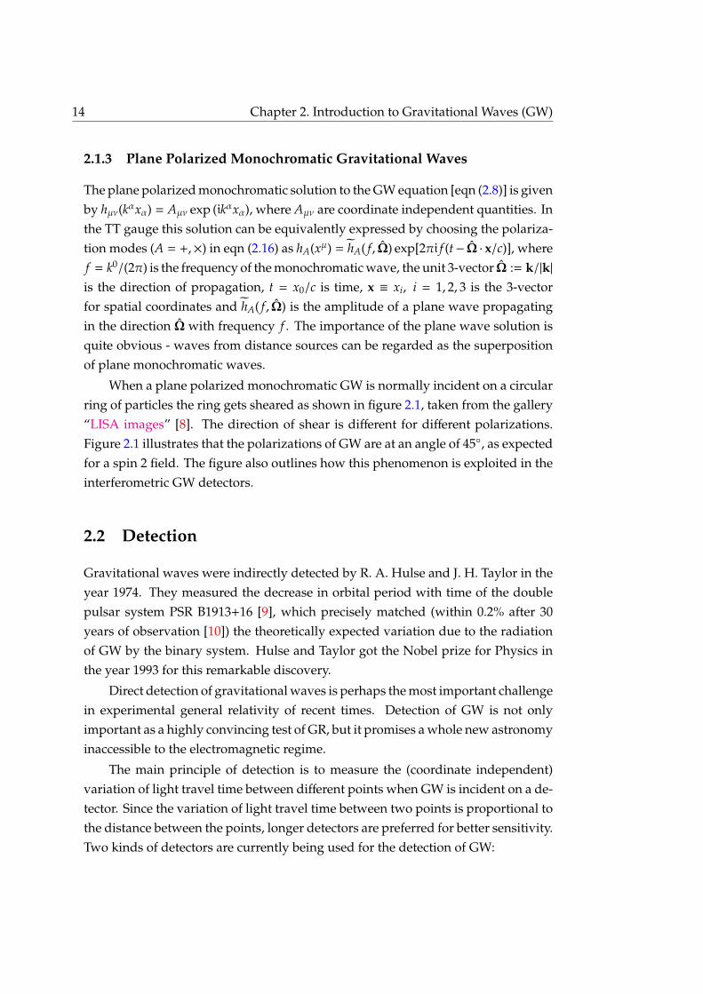
The plane polarized monochromatic solution to the GW equation [eqn (2.8)] is givenby hµν(kαxα) = Aµν exp (ikαxα), where Aµν are coordinate independent quantities. Inthe TT gauge this solution can be equivalently expressed by choosing the polariza-tion modes (A = +,×) in eqn (2.16) as hA(xµ) = hA( f , Ω) exp[2πi f (t− Ω · x/c)], wheref = k0/(2π) is the frequency of the monochromatic wave, the unit 3-vector Ω := k/|k|is the direction of propagation, t = x0/c is time, x ≡ xi, i = 1, 2, 3 is the 3-vectorfor spatial coordinates and hA( f , Ω) is the amplitude of a plane wave propagatingin the direction Ω with frequency f . The importance of the plane wave solution isquite obvious - waves from distance sources can be regarded as the superpositionof plane monochromatic waves.
When a plane polarized monochromatic GW is normally incident on a circularring of particles the ring gets sheared as shown in figure 2.1, taken from the gallery“LISA images” [8]. The direction of shear is different for different polarizations.Figure 2.1 illustrates that the polarizations of GW are at an angle of 45, as expectedfor a spin 2 field. The figure also outlines how this phenomenon is exploited in theinterferometric GW detectors.
2.2 Detection
Gravitational waves were indirectly detected by R. A. Hulse and J. H. Taylor in theyear 1974. They measured the decrease in orbital period with time of the doublepulsar system PSR B1913+16 [9], which precisely matched (within 0.2% after 30years of observation [10]) the theoretically expected variation due to the radiationof GW by the binary system. Hulse and Taylor got the Nobel prize for Physics inthe year 1993 for this remarkable discovery.
Direct detection of gravitational waves is perhaps the most important challengein experimental general relativity of recent times. Detection of GW is not onlyimportant as a highly convincing test of GR, but it promises a whole new astronomyinaccessible to the electromagnetic regime.
The main principle of detection is to measure the (coordinate independent)variation of light travel time between different points when GW is incident on a de-tector. Since the variation of light travel time between two points is proportional tothe distance between the points, longer detectors are preferred for better sensitivity.Two kinds of detectors are currently being used for the detection of GW:

2.2: Detection 15
Figure 2.1: Effect of GW on matter: Detection scheme. When a plane polarizedmonochromatic GW is incident normally on a ring of particles, the ring gets shearedand the direction of shear is dependent on the polarization of the wave as shownin the top panel titled "Two polarizations of GWs". The angle between the twopolarizations is 45, as expected for a spin 2 field. The bottom panel illustrates howthis effect is exploited in the (Michelson) interferometric GW detectors. This figureis taken from the gallery “LISA images” [8].
• Resonant bar detectors: As the name suggests, a detector of this kind isessentially a bar of heavy material. GW, while passing through the bar,excite the near characteristic (resonant) frequency modes of the bar and theseexcitations are read using sophisticated coupled oscillators.
The resonant bar detector made by Weber around 1968 is the first ever GWdetector, though the claim of GW detection [11] using this detector could notbe verified by the scientific community. The present cryogenically cooled bardetectors are much more advanced; many of them in different countries arecurrently operating e.g., ALLEGRO (USA) [12], NAUTILUS (Italy) [13], AU-RIGA (Italy) [14], EXPLORER (Switzerland) [15]. Bar detectors are sensitive

16 Chapter 2. Introduction to Gravitational Waves (GW)
to high frequencies (∼ kHz), so core collapse supernovae are the most promis-ing sources for these detectors. These detectors, in combination to other baror interefometric detectors, are being used to put upper limit on a stochasticbackground. Different omnidirectional shapes, e.g., spherical and “truncatedicosahedral”, for this kind of detectors are also being built. The examplesare MiniGRAIL (Netherlands) [16] and TIGA (USA) [17]. The image of theALLEGRO bar detector at Luisiana State University, is shown in the left panelof figure 2.2 (image taken from “ALLEGRO Archive Photos” [18]).
Figure 2.2: GW Detectors. The left panel shows the ALLEGRO bar detector atLuisiana, US (image taken from “ALLEGRO Archive Photos” [18]). The right panelshows an aerial view of the LIGO detector at Hanford, US. This instrument, in fact,hosts two detectors of 4km and 2km arms (image taken from “LIGO Press & MediaKit: LIGO photos” [19]).
• Interferometric detectors: These detectors are very long (kilometer arm forground based and thousands to millions kilometer for space based) power-recycled Michelson’s inferometers. As illustrated in the previous section,when GW fall on a long Michelson interferometer, the light travel times indifferent arms change, which result in a fringe shift in the output port of theinterferometer. Extracting true GW strain signal from the time series of fringeshifts is the most promising way of detecting GW.
As many as six ground based inteferometric detectors in different countriesare either currently operating or in the commissioning stages, they are: twoLIGO (USA) detectors [20, 21] - at Livingston (LLO) and at Hanford (LHO),TAMA (Japan) [22, 23], GEO (Germany + UK) [24, 25], Virgo (France + Italy)[26, 27] and AIGO of ACIGA (Australia) [28, 29]. The TAMA team is also

2.2: Detection 17
Figure 2.3: LIGO-I sensitivity curves. The noise Power Spectral Densities (PSDs) ofthe LIGO detectors are overlaid on the goal sensitivity of the first generation LIGOdetector. LIGO has reached the goal sensitivity in the fifth science run (S5), whichis on for the last one year. Image taken from the “LIGO Sensitivity” website [32].
making a cryogenically cooled ground based interferometric detector LCGT(Japan) [30, 31].
An aerial view of the LIGO detector at Hanford, USA is shown in the rightpanel of figure 2.2 (image taken from “LIGO Press & Media Kit: LIGO photos”[19]). The ground based interferometric detectors are most sensitive near few100 Hz; coalescing stellar mass inspiraling binaries are the most promisingsources for the interferometric detectors. The sensitivity curves, the plotof square root of noise Power Spectral Density (PSD) with frequency, of theLIGO detectors for different science runs are overlaid on the sensitivity goal infigure 2.3, taken from the “LIGO Sensitivity” website [32]. The LIGO detectorsare operating at the first stage (LIGO-I) goal sensitivity for the last one year.The advanced LIGO sensitivity is targeted within the next few years.
Two space based interferometric detectors, LISA (ESA+NASA) [33,34,35] andDECIGO (Japan) [36], each consisting of three satellites forming a triangular
18 Chapter 2. Introduction to Gravitational Waves (GW)
configuration with huge arm-lengths (5×10⁶ km for LISA and 105 km for DE-CIGO), are also expected within a decade. It is much easier in space to isolatethe low frequency noise, as no seismic vibration is present there. (However,due to the variation of distances between the spacecrafts, the cancellation oflaser frequency noise will require post-processing of detector outputs usingTime Delay Interferometry [37].) LISA and DECIGO will operate in a lowfrequency range (milli-Hertz and deci-Hertz respectively) and hence they areexpected to receive very high energy from high mass binary systems, whichemit at low frequencies. These satellites are also important for putting betterupper limits on the stochastic background. A space based observatory, theBig Bang Observer (BBO) [38, 39], consisting of multiple satellites, is beingplanned as part of NASA’s Beyond Einstein program [40]; it is expected toprecisely measure the cosmological GWB originated during inflation in thevery early universe.
The GW event rate is proportional to the observed volume of space and the am-plitude of GW is inversely proportional to the distance. Therefore, the probabilityof GW detection increases as the cube of sensitivity. Advanced LIGO will undergoabout an order of magnitude improvement in sensitivity as compared to the LIGO-Idetectors; which means that the advanced LIGO detector is thousand times morelikely to detect a GW event, while the event rate for LIGO-I is just one in few years.Thus, the possibility of detection of GW in the next few years is very high.
2.3 Sources and Analysis Strategies
Different kinds of sources generate GW with different frequency spectra. Theanalysis strategies also depend on the kind of sources one is trying to detect. Thethree broad classification of sources and their detection strategies are listed below.
1. Burst: Compact inspiraling binaries in the last few cycles before coalescenceand supernova core collapse release highly energetic GW in very short time.They are called burst sources.
The GW signals from inspiraling binaries have been precisely modeled usingPost-Newtonian approximations [41], hence matched filtering can be used forextracting the true GW signal buried inside strong detector noise. Therefore,the coalescing compact binaries, in particular, the stellar mass binaries whichemit in the sensitive frequency band of the ground based interferometric

2.3: Sources and Analysis Strategies 19
detectors, are the most promising candidates for the detection of GW. Moredetails on the detection strategy of these sources can be found in chapter 3.
On the other hand, the sources like supernovae are unmodeled high frequency(∼ 1 kHz) sources. The analysis strategy to detect such sources makes use ofexcess power statistics technique.
2. Stochastic: Unmodeled and unresolved sources of astrophysical and cosmo-logical origin constitute a stochastic GW Background (GWB). The cosmolog-ical background is analogous the the Cosmic Microwave Background (CMB)and the astrophysical background is analogous to the galactic foreground ob-served while making CMB skymaps. The detection of cosmological GWB willbe a direct probe of inflation and some other important phenomena in theearly universe.
Since the stochastic signals are unmodeled and characterized by their statis-tical expectation values. The best strategy to detect stochastic sources (or putupper limits) is by correlating outputs of two detectors (which can be of differ-ent types - bar and interferometric, say) - forming a GW radiometer. The GWradiometer analysis can be tuned to measure the all sky averaged power of thestochastic background, as well as, to make a sky map of the GWB anisotropy.
The stochastic background is of major interest in this thesis. A more detailedintroduction to the stochastic sources and the complete radiometer analysisare presented in chapter 4, chapter 6 and chapter 7.
3. Continuous: Sources which emit GW continuously over the full observationtime of a detector without significant change in the characteristics are calledcontinuous sources. Asymmetric pulsars and inspiraling binaries, which arenot in the final few cycles before coalescence, are the examples of such sources.
The locations, and also the phase evolutions, of many radio pulsars are quiteprecisely known from electromagnetic astronomy. So a targeted search, bycorrelating signals from two detectors with a time dependent phase factorthat accounts for the light travel time delay between two detectors, is thebest strategy for the detection of GW from known radio pulsars. Search forunknown pulsars is computationally costly, as the parameter space (whichincludes position coordinates) is quite big. The Einstein@Home project [42],in a similar line as the SETI@home project [43], offers a nice solution to utilizeidle computational resources to search for unknown pulsars.

20 Chapter 2. Introduction to Gravitational Waves (GW)
2.4 Summary and Conclusion
Gravitational wave research is reaching new dimensions as the current detectorsare producing science quality data and many ground and space based detectors arecoming up. Brief introduction to the theory, detection, sources and data analysis ofgravitational waves were presented in this chapter.
General theory of Relativity (GR) predicts Gravitational Waves (GW). In theweak field limit GW can be treated as an independent tensor field propagating overa constant (flat) background. GW travel at the speed of light and follows manyother properties similar to the electromagnetic waves, except for polarizations -GW are spin 2 excitations, so the polarization axes are at an angle 45.
GW change the light travel time between different points, which is exploited inthe GW detectors. Two kinds of detectors are currently being used - bar detectorsand interferometric detector. The ground based interferometric detector, LIGO, isoperating at its first stage goal sensitivity for the last one year. Many more groundbased and two space based detectors are coming up within a decade.
Different kinds of sources emit GW, which can be classified in three majorclasses - burst, stochastic and continuous. The analysis strategies for differentsources are also different. Compact inspiraling binaries in the last few cycles beforecoalescence are theoretically well modeled sources, hence matched filtering can beused for these sources. Therefore, the stellar mass compact binaries, which emitin the sensitive bands of the ground based interferometric detectors, are the mostpromising sources for the detection of GW. data analysis strategies for detectingGW signal from inspiraling binaries and stochastic background are principal goalsof this thesis.
The existence of GW has been indirectly established by Hulse and Taylor fromthe observations of the binary pulsar B1913+16. However, the direct detection ofGW is still awaited. Worldwide efforts are being made to detect GW not only toperform a crucial test of GR, they promises a whole new astronomy inaccessibleto the conventional electromagnetic regime. The advanced detectors, scheduledto come up in the next few years, are expected to have a very high probability ofdetection of GW. The detection of GW will be an extremely important achievementin experimental GR. The main goal of this thesis is the development of analysistechniques which can efficiently extract GW signals from the output of the moderngravitational wave detectors.

21
Chapter 3
Search for GW from InspiralingBinaries: Chebyshev Interpolation
Gravitational waves interact weakly with matter, which makes it very difficultto detect. Though the most advanced technologies of microscopic measurementsare being used in the gravitational wave experiments, the detector outputs willbe dominated by noise. However, the sources of gravitational waves, which areexpected to be detected with the modern detectors, have been theoretically modeled.This knowledge can be used to extract signal from noisy data. This is the onlypossible way of detection of gravitational waves using the detectors which arecurrently operating or coming up in the near future.
Inspiraling compact-object binary systems are promising gravitational wavesources for ground and space-based detectors. The time-dependent signature ofthese sources is well-characterized function of a relatively small number of pa-rameters; thus, the favored analysis technique makes use of matched filtering andmaximum likelihood methods. As the parameters that characterize the sourcemodel vary, so do the templates against which the detector data are compared inthe matched filter.
Current analysis methodology samples a bank of filters whose parameter val-ues are chosen so that the correlation between successive samples from successivefilters in the bank is 97%. Correspondingly, the additional information availablewith each successive template evaluation is, in a real sense, only 3% of that alreadyprovided by the nearby templates. The reason for such a dense coverage of param-eter space is to minimize the chance that a real signal, near the detection threshold,will be missed by the parameter space sampling.

22 Chapter 3. Search for GW from Inspiraling Binaries: Chebyshev Interpolation
The current analysis is computationally costly. Efforts are being made to de-velop efficient search algorithms which would allow search over a larger volumeof parameter space with greater number of parameters. For small variations in theparameters, the filter responses are closely correlated. The efficiency of search forinspiraling binaries can be improved by reconstructing the likelihood (or the match)function using sample values of the match function over the parameter space. Wehave investigated the use of Chebyshev interpolation for reducing the number oftemplates that must be evaluated to obtain the same analysis sensitivity [44]. Ad-ditionally, rather than focus on the “loss” of signal-to-noise associated with thefinite number of filters in the template bank, we evaluated the Receiver OperatingCharacteristic, or ROC, as a measure of the effectiveness of an analysis technique.The ROC relates the false alarm probability to the false dismissal probability of ananalysis, which are the quantities that bear most directly on the effectiveness of ananalysis scheme.
As a demonstration we compared the present “dense sampling” analysis method-ology with the “interpolation” methodology using Chebyshev polynomials, re-stricted to one dimension of the multi-dimensional analysis problem by plottingthe ROC curves. We found that the interpolated search can be arranged to have thesame false alarm and false dismissal probabilities as the dense sampling strategyusing 25% fewer templates. Generalized to the two dimensional space used in thecomputationally-limited current analyses this suggests a factor of two increase incomputational efficiency; generalized to the full seven dimensional parameter spacethat characterizes the signal associated with an eccentric binary system of spinningneutron stars or black holes it suggests an order of magnitude increase in compu-tational efficiency. Since the computational cost of the analysis is driven almostexclusively by the matched filter evaluations, a reduction in the number of tem-plates evaluations translates directly into an increase in computational efficiency;additionally, since the computational cost of the analysis is large, the increased effi-ciency translates also into an increase in the size of the parameter space that can beanalyzed and, thus, the science that can be accomplished with the data.
In this chapter, I first give a brief introduction to (Newtonian) Chirp signals. Isummarize the current analysis technique to search for inspiraling binaries basedon matched filtering. Then I mention about the ongoing efforts to develop efficientsearch technique. Rest of the chapter is devoted to the method developed by ususing Chebyshev interpolation and illustrate its efficiency in comparison to thedense search.
3.1: Chirp Signal 23
3.1 Chirp Signal
Inspiraling compact binaries of stellar mass neutron stars or black holes are amongthe most important gravitational wave sources accessible to the current generationof ground-based interferometric gravitational wave detectors [45, 46, 47, 48]. Theyare also very “clean” systems, in the sense that the gravitational wave signal arisingfrom the inspiral depends only on general relativity (eg., the structure of the binarycomponents is unimportant) and can be calculated to great accuracy by the well-understood techniques of post-Newtonian perturbation theory [49, 50, 41].
The gravitational wave signature of inspiraling binary systems depends on aset of 15 parameters that characterize the system (i.e., component masses, orbitalenergy and angular momentum at a given epoch, component spins, orientationrelative to detector line of sight). The signal from inspiraling binaries vary mostrapidly, however, along the axis spanned by the so called “Chirp mass”:
M := µ3/5M2/5, (3.1)
where M is the system’s total mass and µ its reduced mass. For reasons that will beelaborated later, in this work we would only consider the Chirp mass parameter.
The strain response of an interferometric detector due to gravitational wavesincident from an inspiraling binary neutron star system, to quadrupolar approxi-mation, can be written as
h(t|ta, τ0) = h0[π f (t − ta − τ0)M
]2/3 cosΦ(t − ta − τ0), (3.2a)
where
f (t|ta, τ0) :=1πM
(5
256M
τ0 + ta − t
)3/8
, (3.2b)
Φ(t|ta, τ0) := Φa + 2π∫ ta+τ0
tdt f (t|ta, τ0) (3.2c)
for t < ta + τ0. Here ta is the moment when the instantaneous wave frequency isequal to fa and τ0 is the elapsed time from that moment until (in this approximation)the system coalesces, which is directly related to the system’s chirp massM:
τ0 =5
256π fa1(
πM fa)5/3
. (3.3)
24 Chapter 3. Search for GW from Inspiraling Binaries: Chebyshev Interpolation
A typical signal is shown in the top panel of figure (3.1). The amplitude as well asfrequency of the GW signal from inspiraling binaries increase with time, hence theyare often called “Chirp”. The waveform formula given above is calculated usingthe quadrupolar approximation and Newton’s law of gravitation, the signal is thuscalled Newtonian Chirp. Its shape depends only on the Chirp mass parameter.
Chirp signals have been modeled to a vary high degree of accuracy using thepost-Newtonian1 (PN) approximation of order 3.5 — the error in phase variation isless than one in every few thousands cycles, which is the typical number of cycleswhile the frequency of the wave is in the sensitive bands of the modern groundbased detectors. However, like the Newtonian waveforms, very precise Chirpwaveforms are also highly sensitive to the Chirp mass as compared to other physicalparameters characterizing the compact binary. In this work we are interested instudying the relative performances of different search algorithms. We use a onedimensional parameter space to compare the performances of two methods, which,we believe, can be extrapolated to higher dimensions. It is quite obvious that, fora one dimensional analysis, we should consider only the most important intrinsicparameter, the Chirp mass, and the Newtonian Chirp waveform, as its shape isentirely determined by the Chirp mass. This explanation will be repeated in thecontext of computational cost in the next section.
The elapsed time to coalescence τ0 is a useful surrogate for the chirp massM: templates equispaced in τ0 have constant cross-correlation, independent of τ0.Choosing fa equal to 40 Hz, which is commonly taken as the lower-edge of theLIGO detector bandwidth at design sensitivity [51], τ0 ranges from approximately43 s for a binary system consisting of two 1 M compact objects to 0.15 s for a binaryconsisting of two 30 M black holes.
It will soon become clear that working in the frequency domain is quite con-veninent. For neutron star binaries in the LIGO or Virgo band the Fourier transformcan be evaluated to an excellent approximation using the stationary phase approx-imation [52]:
h( f ) = N f−7/6 expi[−Φa − π/4 +Ψ( f |ta, τ0)
], (3.4a)
1Post-Newtonian approximation is a perturbative analysis, where Einstein’s equations are ex-panded as a power series in relative velocity v [using c = 1] of the binary components. The order ofapproximation is defined as the highest power of v2 used in the expansion.

3.2: Dense Search 25
where
Φa = Φ(ta|ta, τ0), (3.4b)
Ψ( f |ta, τ0) = 2π f ta + faτ06π5
(ffa
)−5/3
. (3.4c)
The factorN is a constant amplitude.
3.2 Dense Search
As mentioned in the last section, gravitational waves from inspiraling binaries canbe accurately modeled using general relativity and they are independent of thestructure of the binary components. Because of these reasons matched filtering andmaximum likelihood techniques are well-suited for the detection and characteriza-tion of the signal from these systems [53, 52]. An implementation based on thesemethods is currently used in the analysis of data from the LIGO and GEO detectors(cf. [54, 55, 56, 57]).
3.2.1 Matched Filtering
The above (conventional) search begins with the construction of theoretically mod-eled waveforms or “templates” for discrete points λk on the parameter space λ.[Technically, this process is also called “placement of a template bank over theparameter space”]. The data is then “matched filtered” using the theoreticallyconstructed template bank [58]. For the purpose of the present work we haveλ = τ0, ta,Φa— the chirp mass parameter, the time of arrival and the initial phase.However, as we shall see, it may not be necessary to construct template banksover all the parameters; some parameters can be searched for using sophisticatedmathematical tools, like FFT, consuming very little computation time as describedin [54].
The strain output generated by a gravitational wave detector is a time seriesof real numbers. The Wiener (matched) filter output is the scalar product betweenthe data g(t) and the template h(t). It is convenient to work in the frequencydomain, as the statistical properties of detector noise can be easily characterizedby a frequency power spectrum. Following the Neumann-Pearson approach ofMaximum Likelihood estimation, it can be shown that (cf. [59]) for GW signal frominspiraling binaries the signal-to-noise ratio (SNR) is maximized if we define the

26 Chapter 3. Search for GW from Inspiraling Binaries: Chebyshev Interpolation
scalar product with an inverse noise weight as
⟨g, h
⟩= 4
∫∞
0d f <
g( f )h∗( f )Sn( f )
, (3.5)
where g( f ), h( f ) are the Fourier transforms of g(t), h(t) respectively and Sn( f ) is theone sided power spectral density of detector noise. The basic steps for matchedfiltering can then be listed as below:
1. Evaluate the Wiener filter output W(d|Sn,λk) at each of the template locationsλk;
2. Determine the template λ j whose Wiener filter output is greatest;
3. If the filter output at λ j exceeds the given threshold, report an event with theparameters λ j.
An illustration matched filtering is provided in figure 3.1. A typical chirp signal(top panel), is injected in comparatively stronger noise (middle). The data is thencorrelated with the templates. In this case the templates are also chirp signalsof same shape but with different time of arrivals. The cross correlation value isplotted against the time of arrival. One can see that, when the time of arrival ofthe templates matches that of the injected signal, a very high correlation value isobserved.
3.2.2 Template placement
To choose the template locations we use the match function. Denoting by h(t|λ) thesignal characterized by λ the match Γ(λ j,λk) is
Γ(λ j,λk) =
⟨h(t|λ j), h(t,λk)
⟩√⟨
h(t|λ j), h(t,λ j)⟩〈h(t|λk), h(t,λk)〉
. (3.6)
By construction |Γ| ≤ 1. The templates locations are chosen so that consecutivetemplates in any of the directionsλ j have an overlap Γ0, referred to as the “minimummatch” (MM).
It is also important to distinguish between the nature of the parameters thatcharacterize the template. Changes in some parameters, like τ0, change the shape ofthe Chirp waveform: we term such parameters dynamical parameters (µk). On the

3.2: Dense Search 27
0
2
4
6
8
10
0 0.2 0.4 0.6 0.8 1 1.2 1.4 1.6 1.8 2
Cro
ss c
orre
latio
n
t (sec)
-2e-16
-1e-16
0
1e-16
2e-16
Noi
sy d
ata
-1e-18
-5e-19
0
5e-19
1e-18
Sig
nal h
(t)
Extracting the inspiraling binary signal from noisy data by Matched Filtering
Figure 3.1: Illustration of Matched Filtering. Top: Typical “Chirp” signal due toNewtonian compact binaries. Middle: The above signal is injected into compar-atively strong detector like noise. Bottom: Matched filtering is done over time ofarrival and high correlation is seen when the time of arrival matches the injectiontime of arrival.

28 Chapter 3. Search for GW from Inspiraling Binaries: Chebyshev Interpolation
other hand, parameters, such as ta or Φa, translate the waveform, but do not alterits shape: we term these kinematical parameters2. Maximization of the Wiener filteroutput over the kinematical parameters can be performed in a computationallyefficient manner as shown in the literature [54]. It is not required to search forthe parameters phase Φa and time of arrival ta of the signal by binning thoseparameters and computing the Wiener filter output for each bin. Computationof Wiener filter outputs W(d|Sn,µk, ta, 0) and W(d|Sn,µk, ta, π/2) for two orthogonalphase components Φa = 0, π/2 can be combined together using the formula
W(d|Sn,µk, ta) =√
W(d|Sn,µk, ta, 0)2 +W(d|Sn,µk, ta, π/2)2 (3.7)
to maximize the match over the phaseΦa. The estimate for the signal phase is givenby
Φa = tan−1[W(d|Sn,µk, ta, π/2)
W(d|Sn,µk, ta, 0
]. (3.8)
Also, the Wiener filter outputs for all the time of arrival parameter bins can becalculated at once using fast fourier transform (FFT) technique effectively using thesame amount of computation as required to calculate for just one bin. Therefore,while designing efficient search algorithms, dynamical (intrinsic) parameters areour main concern.
To identify an incident signal using a matched filter requires the application ofa fair sampling of filter templates, each defined by a unique choice of the parametersassociated with the physical system. Current implementations of matched filteringused in the analysis of gravitational wave detector data involves a very densesampling of the two-dimensional parameter subspace corresponding to the binarycomponent masses (intrinsic parameter space) and assuming zero eccentricity orbitsand no body spins. The rationale for choosing a subspace is that the computationalcost of a full parameter space search is high and that many systems are believed to beadequately represented by this subspace. Even for this two dimensional subspacethe minimum computational cost for a matched filter search over component massesin the range 0.2 M < m1 ≤ m2 < 30 M in the LIGO detector band is several hundredGFlops/s [56]. When significant body spin is allowed the computational cost growsby several orders of magnitude [60]. The templates are spaced so closely that thecorrelation between templates at neighboring points in the subspace - the minimal
2In the literature, dynamical and kinematical parameters are also known as intrinsic and extrinsicparameters respectively. Unlike the dynamical parameters, the kinematical parameters can be handledquickly and easily in the filtering algorithms.

3.2: Dense Search 29
match - is 97% [56,55]. We refer to this as the “dense” search strategy. The rationaleunderlying the dense search strategy is to reduce the probability that a weak signal,characterized by parameters that fall between those sampled, will be missed by thesampling3.
Here we are interested in understanding the performance of the different searchstrategies. The current analysis focuses on a two-dimensional parameter spacespanned by the masses of the individual binary components. However, the tem-plates vary most rapidly with the chirp mass. The linear density of templatesneeded by the dense search in the direction ∂M is approximately 100 times the lin-ear density needed in the orthogonal direction. Because of this, for the comparisonof efficiencies we perform here, we focus attention on the number of template eval-uations needed for binaries with equal mass components that vary only inM. Weexpect that the ratio of performance, measured as the number of templates requiredby different search strategies to achieve the same search results, will be the same inthe complementary dimension and in the other dimensions that will be introducedin future searches that accommodate component spins and orbital eccentricity.
3.2.3 Choice of parameter
There are many different ways of parameterizing the template space. Choosingτ0 as a dynamical variable has the advantage that Γ(τ0, τ′0) depends only on thedifference τ0−τ′0; consequently, in the dense search templates are spaced uniformlyin τ0 [54, 55, 56]. To determine that spacing we evaluate
H(∆τ0) = Γ(τ0, τ0 + ∆τ0), (3.9)
where now Γ has been maximized over the kinematical parameters ta and φa. Wecall H the dynamical ambiguity function or simply as the ambiguity function. Itquantifies the fractional match between the template at τ0 and the signal at τ0+∆τ0.Figure 3.2 showsH for power spectral density specified in the initial LIGO sciencerequirements [51]. The requirement thatH(∆τ0) is equal to a constant for any twoconsecutive templates determines the spacing ∆τ0 between templates that differonly in τ0. For our example problem, which has just one dynamical parameter, therequirement thatH(∆τ0) is 97% (the conventional choice) for neighboring templates
3Because the total accessible volume is proportional to the cube of minimum detectable amplitudeand it is assumed that the distribution of detectable sources is uniform in the nearby universe, toensure that at most 10% signals are missed due to the mismatch between data and template, the matchfunction should not fall below 3√1 − 10% ≈ 0.97.

30 Chapter 3. Search for GW from Inspiraling Binaries: Chebyshev Interpolation
0.65
0.7
0.75
0.8
0.85
0.9
0.95
1
-0.1 -0.05 0 0.05 0.1
Am
bigu
ity fu
nctio
n
∆τ0 (sec)
Ambiguity function for Newtonian chirp using LIGO-I SRD with fl=40Hz, fu=512Hz
30ms
60ms
100ms
150ms
200ms
Ambiguity function0.97
Figure 3.2: Ambiguity function. Ambiguity function H plotted as a function of∆τ0. Horizontal lines are drawn for various matches; the dashes horizontal line isfor a 97% match, which corresponds to an inter-template separation of ∼ 30 ms.
leads to a template spacing ∆τ0 equal to 30 ms.
3.3 Efficient Search Algorithms
Dense search is computationally expensive. It is not possible to search over thewhole physically allowed parameter space considering all the parameters with theavailable computing power. Therefore it is extremely important to design efficientsearch algorithms. Several efforts is being made by different research groups todevelop fast data analysis algorithm for the detection of inspiraling binaries. Oneof the very promising method is hierarchical search [61, 62]. In the first stage ofhierarchy a coarse template bank is used with a lower threshold of detection. Inthe subsequent stages, the threshold is increased and a finer search is performedaround the trigger events in the previous stage.
We have developed another4 straightforward and practical way of using in-terpolation to take advantage of the correlation between the matched filter outputassociated with nearby points in the parameter space to significantly reduce the
4Our method can work with the hierarchical search, so this is not an alternative to the hierarchicalscheme, rather, our algorithm can be used to enhance its performance.

3.3: Efficient Search Algorithms 31
number of matched filter evaluations without sacrificing the efficiency with whichreal signals are recognized.
We are not the first to observe the significance of the high correlation betweenneighboring templates nor to consider the opportunity for and advantages of in-terpolation as part of the implementation of matched filtering for the analysis ofbinary inspiral signals. The significance of the high correlation as an indication thatfewer templates should be able to recover signals with the same efficiency, was firstmade in [55]. Croce et al [63, 64] explored the use of Cardinal interpolation with atruncated series of sinc functions to estimate the value of the matched filter outputwhen the filter used corresponds to the actual parameters that describe the signal.They found a sampling of parameter space that would insure the interpolated esti-mate would be no less than 97% of the maximum over a two dimensional intrinsicparameter space. Their sampling and interpolation reduced by a factor of 4, com-pared to the dense search, the number of templates required to search over a twodimensional intrinsic parameter space. Here we find that we can achieve an increasein efficiency by a factor of 3.5 for one dimensional parameter space, with a simplertemplate spacing and a simpler and quicker to evaluate interpolation function.
Cardinal interpolation with sinc functions provides perfect reconstruction ofa band-limited function from equispaced samples. In the present case, however,the function being interpreted is not band-limited and — in any event — we donot have the infinite number of samples that would be required for perfect recon-struction. As an alternative to cardinal interpolation with a truncated series of sincfunctions we consider interpolation using Chebyshev polynomials, which have twoimportant properties: first, they have (very nearly) the minimum maximum errorof all polynomial interpolating expressions of fixed degree; and second, they havethe practical advantage of being quick and easy to calculate. Few more usefulproperties of Chebyshev polynomials have been listed in Appendix A
To understand and demonstrate the performance of the interpolated search weevaluate the both the minimum number of templates required to obtain a givendetection efficiency using both the (Chebyshev) interpolation and dense strategies.We go further, however, and calculate also the false alarm probability of bothsearch strategies. The relationship between the false alarm and false dismissalprobabilities is referred to as the Receiver Operating Characteristic, or ROC. Clearly,given two analysis strategies with the same efficiency, the strategy with the lowerfalse alarm fraction has superior discriminating power. We find that interpolationstrategy using Chebyshev interpolation is superior to the dense analysis strategy or

32 Chapter 3. Search for GW from Inspiraling Binaries: Chebyshev Interpolation
interpolation using the sinc function, from the perspective of either computationalefficiency or discriminating ability.
3.4 Interpolated Search
As discussed in the previous section, the correlation between the Weiner filter out-puts of neighboring templates can be exploited to reduce the number of templateevaluations required to search over the full parameter space. The Wiener filteroutput can be sampled and the full function can be reconstructed using a suitablychosen interpolation scheme. In this section we describe our proposed templateplacement scheme using Chebyshev interpolation and compare it with other rele-vant template placement schemes [44].
3.4.1 Interpolation of the Wiener filter output
The Wiener matched filter W, corresponding to an expected signal characterized byτ , is a scalar-valued function of the (vector-valued) instrument data d, noise powerspectral density Sn:
W(d|τ ) =W(τ |Sn,d). (3.10)
In our particular problem W(d|τ ) is a continuous function of τ and τ correspondsto the intrinsic parameters that characterize our binary system model: e.g., binarysystem component masses, orbital energy and angular momentum, componentspins, etc. Given a data set d we wish to find an interpolating function W(τ ) and aset of points τk in the space of possible signals such that
Wk = W(τk) =W(d|Sn, τk). (3.11)
There are, of course, an infinite number of continuous functions W(τ ) that take onthe values Wk at the τk: the question is, how do we choose among them?
Focus attention first on the case where τ is a scalar x. One particular choice ofinterpolant W(d|Sn, x), which is especially important in the context of communica-tion theory, is based on the Whittaker Cardinal function sinc:
C(x) =∞∑
k=−∞
Wksincx − xk
∆, (3.12)

3.4: Interpolated Search 33
where
sinc(x) =sinπxπx
, (3.13)
xk = x0 + k∆. (3.14)
Shannon [65] showed that the Cardinal interpolation C(x) of W(d|Sn, x) is the uniqueinterpolant W that (i) takes on the values Wk at the xk, (ii) has no singularities, and(iii) and whose spectrum is limited to a bandwidth (2∆)−1. Correspondingly, ifW(d|Sn, x) is bandlimited in x and has the values Wk at the equidistant sampledpoints xk then W(d|Sn, x) is equal to C(x). In the case where τ is multi-dimensionalthe interpolation can be performed separately on each index: e.g., in the case of twodimensions [i.e., τ equal to (τ1, τ2)]
C(τ ) =∞∑
j,k=−∞
W jksincπ∆1
(τ1 − τ1, j
)sinc
π∆2
(τ2 − τ2,k
), (3.15)
where
τ1, j = τ1,0 + j∆1, (3.16)
τ2,k = τ2,0 + k∆2 (3.17)
and τ1,0, τ2,0 are constants.Cardinal interpolation using the Cardinal function sinc forms the basis of the
interpolation formula used in [63, 64]. If W(d|Sn, τ ) is bandlimited and we chooseour samples of W appropriately then we can do no better than using the Cardinalfunction to interpolate values of W between the samples. In our problem, however,W(d|Sn, τ ) is not bandlimited and we do not have an infinite number of samplepoints Wk; correspondingly, the Cardinal function C(τ ) is at best an approximationto W(d|Sn, τ ). With that understanding the Cardinal interpolation C(τ ) is not pre-ferred and we are led to seek other approximations to W(d|Sn, τ ) that have favorableproperties5.
One possibility, chosen from approximation (as opposed to interpolation) the-ory, is the use of a Chebyshev polynomial expansion to approximate W(d|Sn, τ ).Without loss of generality consider a continuous function f (x) on [−1, 1]. The Weier-
5In fact, as noted in [13,14], the Γ is quasi-band-limited: i.e., there exists a Bc such the error one makesby undersampling at frequency B > Bc is proportional to exp[−(B − Bc)]. Nevertheless, interpolationwith the Cardinal function is still an approximation and, as we are about to see, other interpolatingfunctions can achieve equivalent accuracy at smaller computational costs.

34 Chapter 3. Search for GW from Inspiraling Binaries: Chebyshev Interpolation
strass Approximation Theorem states that for any ε > 0 we can find a polynomialPn of order n such that
maxx∈[−1,1]
∣∣∣ f (x) − Pn(x)∣∣∣ ≤ ε. (3.18)
The minimax polynomial approximation to W(d|Sn, x) is a natural candidate forthe interpolation W(x). Unfortunately, finding the minimax polynomial is a verydifficult process; nevertheless an excellent approximation to the minimax polynomialdoes exist. Define the error E(x| f ,Pn) associated with the polynomial approximationPn(x) by
E(x| f ,Pn) ≡ f (x) − Pn(x). (3.19)
The Chebyshev Equioscillation Theorem [66] states P∗n is the minimax polynomialif and only if there exist n + 2 points −1 ≤ x0 < x1 < · · · < xn+1 ≤ 1 for which
E(xk| f ,P∗n) = (−1)kE, (3.20)
where|E| ≡ max
x∈[−1,1]
∣∣∣E(x| f ,Pn)∣∣∣ . (3.21)
As a corollary, E(x| f ,P∗n) vanishes for x ∈ [−1, 1] at n+1 points x′k, with xk < x′k < xk+1.This result, together with the Mean Value Theorem, allows us to write the error termassociated with the minimax polynomial P∗n as
E(x| f ,P∗n) =f (n+1)(ξ)(n + 1)!
n∏k=0
(x − x′k), (3.22)
where ξ ∈ [−1, 1]. Correspondingly,
|E| ≤ maxx∈[−1,1]
∣∣∣∣∣∣∣n∏
k=0
(x − x′k)
∣∣∣∣∣∣∣ maxξ∈[−1,1]
∣∣∣ f (n+1)(ξ)∣∣∣
(n + 1)!. (3.23)
Focus attention on the order n + 1 polynomial
Q∗n+1(x) =n∏
k=0
(x − x′k). (3.24)
This polynomial has leading coefficient unity. A unique property of the Chebyshevpolynomial Tn+1 is that, of all order n+ 1 polynomials Qn+1 with leading coefficient

3.4: Interpolated Search 35
unity,
maxx∈[−1,1]
∣∣∣∣∣Tn(x)2n−1
∣∣∣∣∣ ≤ maxx∈[−1,1]
|Qn+1(x)|. (3.25)
Additionally, Tn+1(x) has exactly (n + 2) extrema on [−1, 1], the value of |Tn+1(x)| atthese extrema is 1, and the extrema alternate in sign. Correspondingly, if the errorterm E(x| f ,P∗n) associated with the minimax polynomial P∗n were polynomial — i.e.,f (n+1)(ξ) were constant in equation 3.22 so that E(x| f ,P∗n) was equal to Q∗n — then bythe Equioscillation Theorem Q∗n+1 would be equal to Tn+1 and the x′k — where theerror vanishes — would be the n + 1 roots of Tn+1. This suggests that we find theorder n polynomial p∗n such that
p∗n(x′k) = f (x′k) ∀ k = 0 . . . n (3.26)
where, again, the x′k are the roots of Tn+1. The polynomial p∗n is a near minimaxpolynomial approximation to f (x). For this polynomial approximation Powell [67]showed that, as long as f (x) is continuous on [−1, 1],
1 ≤εcheb
ε0≤ νn ≡ 1 +
1n + 1
n∑k=0
tan[(k + 1/2)π
2(n + 1)
]. (3.27)
where
ε0 = maxx∈[−1,1]
∣∣∣E(x| f ,P∗n)∣∣∣ , (3.28)
εcheb = maxx∈[−1,1]
∣∣∣E(x| f , p∗n)∣∣∣ . (3.29)
Powell also showed that νn grows slowly with n: in particular,
νn ∼2π
log n. (3.30)
Somewhat tighter bounds on νn can be placed when f is differentiable [68].
As defined above, the near minimax polynomial p∗n is the interpolating poly-nomial that agrees with f at the n + 1 roots of Tn+1. Alternatively, using severalproperties of Chebyshev polynomials, the Chebyshev interpolating polynomial canbe expressed as a linear combination of Chebyshev polynomials:
p∗n(x) =n∑
k=0
akTk(x) −12
a0, (3.31)

36 Chapter 3. Search for GW from Inspiraling Binaries: Chebyshev Interpolation
where
a j =2
n + 1
n+1∑k=1
f (x′k)T j(x′k), (3.32)
where, again, the x′k are the n + 1 roots of Tn+1.
3.4.2 Search strategy
Following the above discussion we are in a position to describe an alternativestrategy, which we refer to as the interpolated search strategy.
Here also we first describe the general strategy using the full set of parametersλ. However, as was in the case of dense search, we may not have to place templatebanks over all the parameters. In the present case, we use interpolated search onlyfor the dynamical parameter6, namely the Chirp mass τ0, and maximize over thekinematical parameters, the time of arrival ta and the initial phaseΦa, using the fastFFT based method described in [54].
The general scheme is as follows. First, fix the order of the interpolatingpolynomial. This determines the template locations λk on the parameter space λ.Then
1. Evaluate the Wiener filter W(d|Sn,λk) at each of the template locations λk;
2. Form the interpolating polynomial from the W(d|Sn,λk);
3. Determine the location λ′ where the interpolating polynomial is maximized;
4. Perform a final Wiener filter evaluation at λ′;
5. If the final evaluation exceeds the given threshold, report an event with theparameters λ′.
We illustrate the interpolated search strategy using Fig. 3.3. In Fig. 3.3 weuse 37 interpolating search templates, that is, we sample the ambiguity function at37 points in the τ0 space (the marked points on the dotted curve). We constructthe interpolating function (the solid curve) and find its maximum by setting itsderivative to zero. In order to avoid local extrema, we first find the approximatelocation of the peak of the interpolating function and then find the zero of its
6Note that, interpolation over kinematical parameters may also improve the performance of thesearch algorithms [55]. Although this case has not been considered in the work presented here, it isworth exploring the possibility in future efforts to maximize the efficiency to search for the binaryinspirals.

3.4: Interpolated Search 37
-6
-4
-2
0
2
4
6
13.5 14 14.5 15 15.5
Der
ivat
ive
τ0 (sec)
Derivative of interpolated Ambiguity function
0.2
0.3
0.4
0.5
0.6
0.7
0.8
0.9
1
Am
bigu
ity fu
nctio
n
37 templates over the range τ0=13-17sec and a test signal placed at 14sec
Actual Ambiguity functionSampled points
Interpolated Ambiguity functionObserved match
Figure 3.3: Illustration of Interpolated Search. This figure demonstrates the in-terpolated search. The ambiguity function is sampled and reconstructed over thechosen parameter space of τ0 = 13 − 17 sec (only a part of the parameter space hasbeen shown in the figure) with the help of the Chebyshev interpolating polynomial.The approximate location of the peak of the interpolating function is first locatedand the zero of the derivative is obtained by applying successive approximationsaround the peak. Finally a template is placed at this estimated signal location. Notethat by placing a template at the maximum of the interpolating polynomial, thematch has improved over the one obtained by simply evaluating the maximum ofthe interpolating polynomial.

38 Chapter 3. Search for GW from Inspiraling Binaries: Chebyshev Interpolation
derivative by successive approximation near the region of the peak. One canclearly see that the proper value of the ambiguity function at the maximum ofthe interpolating function is more than the maximum value of the interpolatingfunction and this is what we gain by placing a template at the maximum of theinterpolating function.
3.4.3 Template placement
In the dense search templates are equispaced in τ0, with the spacing betweenadjacent templates — and thus the number of templates — chosen such that thedynamical ambiguity function takes on a specified value. When presented withdata an event is signaled when the amplitude at one of these templates exceeds athreshold.
In the interpolated search, on the other hand, the domain [τmin0 , τmax
0 ] is mappedonto [−1, 1] and the placement and number of templates is chosen to simplify theconstruction of the Chebyshev interpolating polynomial of the template outputover this domain. When presented with data the maximum value of the Chebyshevinterpolating polynomial is found and an event is signaled when the amplitude atthat location exceeds a threshold.
In the interpolated search our goal is to minimize the order of the interpolatingpolynomial (and, thus, the number of template evaluations) required for a givenaccuracy of interpolation. We have some control over this through the choice ofmapping from [τmin
0 , τmax0 ] to [−1, 1]. The linear map
τ′ = 2τ0 − τmin
0
τmax0 − τmin
0
− 1, (3.33)
is the most obvious such mapping. While have not made an exhaustive search ofall possible mappings; however, we have observed that better fits are possible witha lower-order polynomial when we use the mapping
δ = cos(τ′) = − cos
π τ0 − τmin0
τmax0 − τmin
0
. (3.34)
Moreover, with this mapping, the roots of the Chebyshev polynomial are equi-spaced7 over the parameter range in τ0. Note that the Chebyshev polynomials
7This means that the Wiener filter outputs from a conventional dense search can also be used asinput to the Chebyshev interpolation scheme to yield a better efficiency by performing negligible

3.4: Interpolated Search 39
can also be written as Tn(x) = cos[nθ(x)], where x = cosθ, so in this case Tn(δ) =cos(nπτ′). Since the τ′ space is sampled uniformly due to the above mapping,Chebyshev interpolation is now equivalent to a type II Discrete Cosine Transformin πτ′. Equispaced sampling of the parameter space could be beneficial if thesignals are distributed uniformly over the τ0 space. Nevertheless, for a nonuniformdistribution of signals, different transformation could be preferred to give optimumresults. Once we have fixed the order n of the interpolating polynomial, templatesare placed at values of δ that are roots of the Tn+1(δ). This fixes the templates. Thecoefficients of the interpolating polynomial are found using equation 3.32 and thenthe interpolating polynomial is constructed using equation 3.31.
It is obvious that minimum number of templates should be used for maximumcomputational advantage. We choose the order of interpolation n to be the minimumorder that can retain the MM of 97%. This is equivalent of saying that any injectedsignal should be located within the error window where the ambiguity functioncentered about the injection point is above the MM. So, in our case, the error inlocating any signal should be less than 15 ms. To do this, we first inject a normalizedsignal at a non-special location of the parameter space. The order of interpolationis then varied over a reasonable range of value and the error (bias) in locating thesignal is noted for each order. This variation has been plotted in figure 3.4. Theminimum order for which the bias is less than 15 ms gives a lower limit to thenumber of templates to be used. From the figure one can see that the number is35. We, then, increase the number of templates and find the minimum number forwhich the maximum match is greater than 97% for any injection point. By performingthis exercise, we get the minimum oder of interpolation required to retain the MMof 97% for the parameter space considered here is 37.
In figure 3.5 we have plotted the match by placing normalized test signals(without noise) at regular intervals of τ0. For each injected signal τ0, we plot themaximum of the interpolating polynomial (dashed curve) and the match obtainedby placing a template at the maximum of the interpolating polynomial (solid curve).We see that the match is a (nearly) periodic function of τ0, with the period equal tothe template separation. This suggests that the detection probability is also periodicand this fact has been used in carrying out the simulations - the signals are injectedwithin one such “period" in the parameter space. Moreover, one can see that withjust 37 + 1 interpolated search templates one gets a MM of 0.97, whereas the densesearch requires about 133 templates to achieve the same level of MM. This amounts
amount of extra computation.

40 Chapter 3. Search for GW from Inspiraling Binaries: Chebyshev Interpolation
-0.03
-0.025
-0.02
-0.015
-0.01
-0.005
0
0.005
0.01
0.015
0.02
0.025
20 30 40 50 60 70
Bia
s (s
ec)
Order of interpolating Chebyshev polynomial
Variation of error (bias) in estimating the position ofa signal at τ0=14.0sec with interpolation order
Bias (sec)±15ms
Figure 3.4: Variation of bias with no. of interpolated search templates. A nor-malized test signal (without noise) was injected at a non-special location on theparameter space. The error occurred in locating the signal position (bias) is plottedwith the number of templates. This plot gives an indication about the number oftemplates required to keep the bias less than 15 sec, so that, the minimal match doesnot fall below 97%. One can see that at least 35 templates are needed to keep theminimal match greater than 97%. See text for the next steps to fix the exact numberof templates.

3.4: Interpolated Search 41
0.85
0.9
0.95
1
1.05
13.7 13.8 13.9 14 14.1 14.2 14.3
Est
imat
ed m
axim
um o
f am
bigu
ity fu
nctio
n
Signal τ0
Performance of the Interpolated Search scheme in terms of Minimal Match for LIGO-I SRD with 37 templates
Max of interpolated ambiguity fnAmbiguity fn at estimated signal position
0.97Templates position
Figure 3.5: Variation of Match with signal location. Normalized test signals (with-out noise) were injected densely at regular intervals along the τ0 parameter space.For each injected signal τ0, we plot the maximum of the interpolating polynomial(dashed curve) and the match obtained by placing a template at the maximum of theinterpolating polynomial (solid curve) according to the interpolated search strategy.This figure illustrates that the match is a (nearly) periodic function of τ0 with theperiod equal to the template separation. Moreover, with just 37 + 1 interpolatedsearch templates the minimal match is 0.97. To maintain the same minimal match133 templates are needed for the usual dense search.

42 Chapter 3. Search for GW from Inspiraling Binaries: Chebyshev Interpolation
to a factor of 3.5 over the dense search and this is so for just one dimension. Note that,the gain factor obtained by Croce et al. in [63] is ∼ 4 in two dimensions, which scalesto ∼ 2 per dimension. Because the metric (Fisher information matrix) determinesthe lattice spacing as well as the correlation, they are interdependent. This suggeststhat the Chebyshev interpolation method can be extended to a parameter space ofhigher dimensions with about a similar gain factor per dimension.
3.5 Comparison between Dense and Interpolated search:ROC curves
In this section we compare the performances of the dense and interpolated searchstrategies when applied to the problem of identifying the gravitational wave signa-ture of coalescing neutron star systems in the LIGO detectors.
We are interested in two, related, comparisons: first, the relative “sensitivity”of a search carried-out with a fixed number of template evaluations using thedense search strategy and the interpolated search strategy; second, the number oftemplate evaluations required by the interpolated search in order to achieve thesame “sensitivity” as the dense search. To give meaning to the “sensitivity" of thesetwo strategies we use the Receiver Operating Characteristic, or ROC.
The ROC is a plot of true positives as a function of the fraction of false positivesfor a binary classifier system as its discrimination threshold is varied. Both thedense search and the interpolated search are binary classifiers: i.e., they classify aninterval of data d as including a signal or not including a signal. A true positiveis a classification of d as including a signal when in fact it does; a false positive isa classification of d as including a signal when it does not. In both of the searchstrategies described here the discrimination threshold is matched filter output thatmust be exceeded for a data interval to be classified as including a signal. The falsepositive fraction is also known as the type II, or false alarm, error fraction and isdenoted α. The fraction of true positives is also known as the detection efficiencyε, which is one minus the type I, or false positive, error fraction (which is denotedβ). At fixed α a more sensitive search method has a greater ε. The ROC associatedwith a search method no better than a toss of a (possibly loaded) coin is given bythe diagonal α = ε.
Using numerical simulations we have evaluated α and ε as a function of thedetection threshold for both the interpolated search and the dense search, for dif-ferent numbers of templates (dense search) and different interpolating polynomial

3.5: Comparison between Dense and Interpolated search: ROC curves 43
order (interpolated search).
To evaluate the false positive fraction α we generate a large number of datasegments, each 215 samples long, and each consisting of Gaussian noise whosepower spectrum (assuming a 1024 Hz sample rate) is that specified as the initialLIGO science requirement [51]. (The Gaussian random numbers are themselvesgenerated using the Mersenne Twister Pseudo Random Number Generator [69]and then filtered in the Fourier domain by scaling the Fourier components by thesquare root of the PSD.) For the purpose of this comparison we look for signals inthe interval τ0 ∈ [13 s, 17 s]. Both the dense and interpolated search methods areapplied to this data. The ratio of the number of events signaled to the number ofdata segments examined as a function of the threshold η is α for that threshold.Approximately 50,000 realizations of detector noise are used to evaluate α, whichgives reliable results for α greater than approximately 10−3.
To compute ε, the true positive fraction, we proceed in a similar fashion. Now,however, with each noise instantiation we add a signal, with τ0 drawn uniformlyand randomly from the interval covered by the search: i.e., τ0 ∈ [13 s, 17 s]. Weinject signals of SNR 8. In almost all cases 50, 000 realizations of detector noise plussignal are used to evaluate the efficiency, which gives reliable results for efficienciesgreater than approximately 10−3. However, for the flat search with 40 templatesand the interpolated search with 30 templates,we have used 400, 000 realizations.The larger number of realizations in these cases results in smoother curves.
The top panel of Fig. 3.6 shows the variation of α for both methods using 40templates: i.e., a 100 ms template spacing for the dense search and an order 39interpolating polynomial in δ (cf. equation 3.34). For any threshold α is alwaysgreater for the dense search than for the interpolated search; similarly, as shown inthe center panel of Fig. 3.6, for any given threshold the efficiency ε is always greaterfor the interpolated search than for the dense search. Finally, the bottom panel ofFig. 3.6 shows the ROC for a 40 template dense search and an order 39 interpolatedsearch, both of which involve 40 template evaluations to decide if a signal has beendetected. Comparing both ROCs it is clear that the interpolated search is moresensitive at any given α then the dense search. This is always true: i.e., for a fixednumber of template evaluations the interpolated search will always have a betterefficiency at a given α than the dense search, though as the number of templatesgrows large the fractional difference in sensitivity will decrease.
Figure 3.7 and table 3.1 addresses the second of our two questions: the numberof templates evaluations required of an interpolated search to have the same sensi-

44 Chapter 3. Search for GW from Inspiraling Binaries: Chebyshev Interpolation
Table 3.1: Comparison between dense and interpolated search. Number of tem-plate evaluations required to obtain the same efficiency at a false alarm fraction of10−3 in a dense search and an interpolated search. Note how the interpolated searchis computationally more efficient for the same sensitivity.
# templatesε at α = 10−3
Dense Interp.40 31 0.85950 41 0.89060 49 0.90580 64 0.919
100 89 0.924140 105 0.927160 115 0.929
tivity as a dense search. Figure 3.7 shows the ROCs for dense searches using 140 and160 templates, together with the ROCs for interpolated searches using 120 and 100templates. The interpolated search with and order 120 interpolating polynomial isclearly as sensitive as a dense search with 160 templates, and an interpolating searchwith an order 100 polynomial is as sensitive as a dense search with 140 templates.Table 3.1 shows similar pairings of the number of templates in a dense search andthe number of templates in an interpolating search necessary to achieve the samesensitivity.
3.6 Summary and Conclusion
Inspiraling binaries are the most promising sources for the currently operating andupcoming gravitational wave detectors. Signals from these detectors will be dom-inated by instrumental noise. However, the signals from the inspiraling binariescan be accurately modeled using (approximate theories of) general relativity andthese signals do not depend on their internal structures of the binary components.This makes it possible to detect the signals using matched filtering and maximumlikelihood techniques.
The existing data analysis algorithm, that is being used for the analysis of LIGOand GEO data, considers only two mass parameters of the binary and denselyplaces templates over this parameter space so that signals are not missed out ifthey fall in between two templates. We call this “dense” search. Dense search iscomputationally expensive and it is extremely difficult with the available computing

3.6: Summary and Conclusion 45
0
0.1
0.2
0.3
0.4
0.5
0.6
0.7
0.8
0.9
1
3.5 4 4.5 5 5.5 6 6.5 7
Fal
se a
larm
pro
babi
lity
Threshold (η)
Comparison between false alarm probability vs. threshold curves
FS: 40 templatesIS: 40 templates
0
0.2
0.4
0.6
0.8
1
2 4 6 8 10 12 14
Fal
se d
ism
issa
l pro
babi
lty
Threshold (η)
Comparison between false dismissal probability vs. threshold curvesfor injected SNR=8
FS: 40 templatesIS: 40 templates
Figure 3.6: Comparison: False Alarm & False Dismissal probability. The variationof the false and true positive fractions, α and ε with threshold η for the denseand interpolated search methods, each making use of 40 template evaluations.The top panel shows the false positive fraction. Note how the false positive fallsmuch sooner for the interpolated search than for the dense search. The bottompanel shows ε when a signal of amplitude signal to noise 8 is present in the rangeτ0 ∈ [13 s, 17 s]. Note how the ε is always greater for the interpolated search than forthe dense search. For the same computational cost (determined by the number oftemplate evaluations) the interpolated search will always perform better than thedense search.
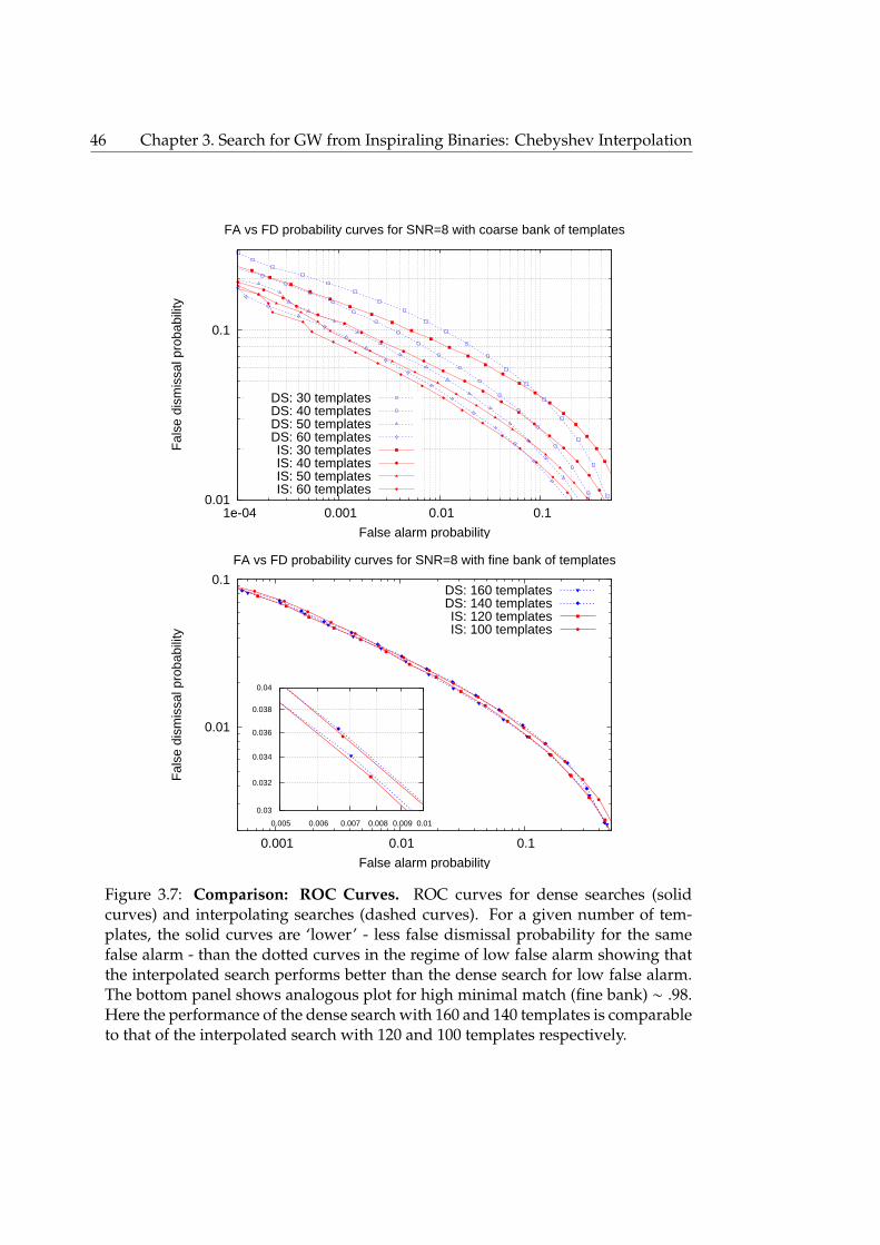
46 Chapter 3. Search for GW from Inspiraling Binaries: Chebyshev Interpolation
0.01
0.1
1e-04 0.001 0.01 0.1
Fal
se d
ism
issa
l pro
babi
lity
False alarm probability
FA vs FD probability curves for SNR=8 with coarse bank of templates
DS: 30 templatesDS: 40 templatesDS: 50 templatesDS: 60 templatesIS: 30 templatesIS: 40 templatesIS: 50 templatesIS: 60 templates
0.01
0.1
0.001 0.01 0.1
Fal
se d
ism
issa
l pro
babi
lity
False alarm probability
FA vs FD probability curves for SNR=8 with fine bank of templates
DS: 160 templatesDS: 140 templatesIS: 120 templatesIS: 100 templates
0.04
0.038
0.036
0.034
0.032
0.03
0.01 0.009 0.008 0.007 0.006 0.005
Figure 3.7: Comparison: ROC Curves. ROC curves for dense searches (solidcurves) and interpolating searches (dashed curves). For a given number of tem-plates, the solid curves are ‘lower’ - less false dismissal probability for the samefalse alarm - than the dotted curves in the regime of low false alarm showing thatthe interpolated search performs better than the dense search for low false alarm.The bottom panel shows analogous plot for high minimal match (fine bank) ∼ .98.Here the performance of the dense search with 160 and 140 templates is comparableto that of the interpolated search with 120 and 100 templates respectively.

3.6: Summary and Conclusion 47
resources to search over all the parameters and the full volume of the parameterspace using dense search.
We have shown that the use of near-minimax interpolating polynomials to fitthe output of matched filters to the filter parameter values can greatly improve thesensitivity of a matched-filter based search for gravitational waves from compactbinary inspiral. Since the lattice for dense search and the correlations are depen-dent on the metric (Fisher information matrix) and any interpolation exploits thesecorrelations, we believe that the Chebyshev interpolation method can be extendedto a parameter space of higher dimensions with about a similar gain factor perdimension. Using such a polynomial to find the parameters of the signal templateleading to the best match we can reduce the computational cost of a search overa two dimensional parameter space by a factor of two compared to the methodscurrently in use, without any loss of sensitivity or discriminating power. This fac-tor of two becomes a factor of ten when the search is over the seven dimensionalparameter space that includes not only the masses but also the spins of the binarycomponents [70]. This savings in computational cost is estimated under the as-sumption, which we believe well-founded, that we will obtain the same savingswhen the interpolation is extended to additional dimensions.
Moreover, the scheme we have developed places templates uniformly overthe parameter space, like the current dense search. So the Wiener filter outputs ofthe dense search can be used as input to the Chebyshev interpolation and betterefficiency can be achieved by performing negligible amount of extra computation.
Other suggestions have been made for reducing the number of filter evalua-tions without sacrificing detection efficiency. One promising proposal involves ahierarchical search strategy, wherein a low-threshold trigger generated by the eval-uation of the matched filters associated with a much coarser sampling of parameterspace followed by (if necessary) a higher threshold evaluation matched filters overa much finer sampling of parameter space [61,71,72,73,62]. The interpolation strat-egy we describe here can be implemented together with the hierarchical strategiesto further improve the computational efficiency of binary inspiral analysis. Whilethe gain in efficiency of the interpolated search over the dense search is approx-imately constant in the desired false alarm probability, the balance between thecoarseness of the grids in the hierarchical steps, the number of hierarchical steps,and the gain in computational efficiency associated with the interpolation is notobvious and requires further study. Nevertheless, since the major contribution tothe computational cost of a multi-grid search is thought to arise in the initial stage

48 Chapter 3. Search for GW from Inspiraling Binaries: Chebyshev Interpolation
of the search, the gain in computational efficiency — and, correspondingly, the sizeof the parameter space that can be studied with fixed computational resources —could be substantial.

49
Chapter 4
Search for GW Background(GWB): Radiometer Analysis
The universe is expected to have a stochastic Gravitational Wave Background (GWB)of astrophysical and cosmological origin. Incoherent superposition of unmodeledand/or unresolved sources of GW, which are characterized by statistical expecta-tion values, constitute the stochastic GWB. The cosmological GWB component isanalogous to the Cosmic Microwave Background (CMB) - a stochastic backgroundof electro-magnetic radiation, whereas the GWB component generated from astro-physical sources, e.g., supernovae, binaries etc., is analogous to the foregroundobserved in CMB experiments, which will generally be higher in amplitude fromthe GWB of cosmological origin. Different types of astrophysical and cosmologicalsources of GWB and their modeled frequency spectra have been listed in section 4.2.Measurement of the strength of the statistically isotropic cosmological GWB willbe a direct probe of inflation and some other important phenomena in the earlyuniverse.
As the noise streams in different instruments are independent, the cross-correlation between the data from a pair of detectors is the best statistic for theestimation of the strengths of stochastic signals. The cross-correlation statistic canbe used to measure the sky averaged strength of the GWB [74, 75, 76], as well as, tomake skymap of the GWB [77, 78, 79, 80, 81, 82] using the ground and space baseddetectors. In order to “point” a baseline formed by a pair of detectors at different lo-cations, a time dependent phase delay is introduced in the cross-correlation statisticthat accounts for the light travel time delay between the detector sites for a givensource direction. As the earth rotates, the phase factor is adjusted in such a way

50 Chapter 4. Search for GW Background (GWB): Radiometer Analysis
that the signal from the pointing direction is coherently added, while the signalsfrom other directions wash out. The phase delay, however, is introduced througha filter function, which also takes into account the variation of source power spec-tral density (PSD) and non-stationary detector noise PSD over different frequencybands. The filter function can be altered to search for different models of stochasticbackgrounds.
The method of synthesis imaging using the rotation of the earth is well devel-oped in radio astronomy and CMB analysis. A similar approach is used here, forthe first time, to propose a method for mapping the GWB and, hence, the analysisis called “GW radiometer”. The general GW radiometer framework is presented insection 4.3 to search for any model of GWB. Two important “blind” estimations -the search for a isotropic background and to map the GWB sky - have been outlinedin section 4.4.
Blind estimations of the upper limits on the strengths of a isotropic GWBand a stochastic point source using a GW radiometer formed by the pair of LIGOobservatories at Hanford and Louisiana have already been implemented [83,84,85].The upper limit on the sky averaged stochastic GWB obtained from the fourth LIGOscience run data is currently the best in the frequency range 51 − 150Hz [84].
4.1 Stochastic Gravitational Wave Background (GWB)
A gravitational wave in the weak field limit can be treated as an external field overa flat Minkowski background:
ds2 = − c2 dt2 + dx2 + hab(t, x) dxa dxb (4.1)
where the roman indices a, b run from 1 to 3. In the transverse traceless (TT) gaugethe metric perturbations h(t, x) ≡ hab(t, x) can be expanded in terms of plane wavesof the two polarizations A = +,×
h(t, x) =∑
A=+,×
∫∞
−∞
d f∫
S2dΩ hA( f , Ω) eA(Ω) e2πi f (t−Ω·x/c), (4.2)
where a tilde (˜) above a variable denotes its Fourier transform, the complex Fourieramplitudes satisfy the relation h∗A( f , Ω) = hA(− f , Ω) owing to the reality of h(t, x),

4.1: Stochastic Gravitational Wave Background (GWB) 51
Ω is a unit vector on the two sphere with spherical polar coordinates (θ, φ)
Ω = cosφ sinθ x + sinφ sinθ y + cosθ z (4.3)
and the polarizations tensors eA(Ω) ≡ eAab(Ω) are defined by the following equations
m(Ω) := sinφ x − cosφ y (4.4a)
n(Ω) := cosφ cosθ x + sinφ cosθ y − sinθ z (4.4b)
e+(Ω) := m(Ω) ⊗ m(Ω) − n(Ω) ⊗ n(Ω) (4.4c)
e×(Ω) := m(Ω) ⊗ n(Ω) + n(Ω) ⊗ m(Ω). (4.4d)
Stochastic signals can not be modeled as a time series, they are characterizedby their expectation values. If we assume a stochastic GWB without any correlationbetween different polarizations1, frequencies and directions2 we may write
〈h∗A( f , Ω) hA′( f ′, Ω′)〉 = δAA′ δ( f − f ′) δ2(Ω − Ω′)PA(Ω) H( f ), (4.5)
wherePA(Ω) is proportional to the strength of the GWB in the direction Ω and H( f )is the two sided GW source Power Spectral Density (PSD).3 The quantityPA(Ω) maybe properly interpreted by comparing it with the total GW energy density.
The total GW energy density ρGW(t, x) can be defined as [2, 76]
ρGW(t, x) =c2
32πG〈h(t, x) : h(t, x)〉, (4.6)
where a dot ( ˙ ) represents derivative with respect time t and a colon ( : ) rep-resents the matrix contraction operation. For a stochastic background ρGW(t, x) is
1It is important to note that, even if the polarizations are independent in certain direction, therecan be mixing between polarizations in the other directions due to the rotation of the basis vectors.This complication has not been included in this thesis, because for numerical applications we onlyconsider equal power in both the polarizations where this complexity does not arise. However, itshould be straight forward to include this phenomenon in the analysis framework presented here.
2The inflationary GWB will have angular correlations over angular scales larger than the angularresolution of the radiometers formed using the ground based detectors. Development of a moregeneral analysis technique to incorporate the angular correlations in GWB is being planned.
3In general, we can not separate H( f ) from PA(Ω), because the frequency power spectrum H( f )could also depend on the direction Ω. A more general treatment would use
〈hA( f , Ω) hA′ ( f ′, Ω′)〉 = δAA′ δ( f − f ′) δ2(Ω − Ω′)PA(Ω, f ),
where PA(Ω, f ) describes both frequency and angular distribution of GWB power together.

52 Chapter 4. Search for GW Background (GWB): Radiometer Analysis
statistically stationary and, in practice, it should not vary significantly over theneighborhood of earth where we can place the detectors. Hence, from now on, weomit the arguments (t, x) from ρGW(t, x).
In cosmology, energy density of a component is usually represented by itsrelative magnitude with respect to the cosmological critical density ρcrit requiredfor a flat universe,
ρcrit =3 c2 H2
0
8πG, (4.7)
(in the units of energy density) where H0 is Hubble constant at the current epoch.If the GWB is statistically homogenous and stationary4, the energy density of theGWB ρGW is uniform over the whole universe, hence the energy density is betterrepresented by its relative strength ΩGW with respect to the critical density
ΩGW :=ρGW
ρcrit. (4.8)
The frequency spectrum of GWB energy density is also a very important phys-ical quantity. The community has adopted the notation ΩGW( f ) to represent theone sided frequency spectrum, which should not be confused with its all frequencyintegrated counterpart ΩGW. The frequency spectrum of GWB produced by slowroll inflation, a very important pillar of standard big bang cosmology, is scale in-variant, i.e., flat in logarithmic frequency scale. Therefore, conventionally, the GWBspectrum is defined as the energy density per unit logarithmic frequency interval
ΩGW( f ) := limδ ln f→0
[1ρcrit
δρGW
δ ln f
]f, (4.9)
where δρGW is the contribution to the energy density from the infinitesimal loga-rithmic frequency interval δ ln f at frequency f (for an alternative but equivalentdefinition of ΩGW( f ) see, e.g., [86]). If we define a cumulative spectrum of energydensity ρGW( f ) as the one sided total energy density contributed by the frequencyinterval [0, f ], so that, ρGW(∞) ≡ ρGW, we can express the spectrum as a properlogarithmic derivative:
ΩGW( f ) =1ρcrit
dρGW( f )d ln f
. (4.10)
If the frequency spectrum ΩGW( f ) is integrated over all the (logarithmic) frequen-
4Though the energy density ρGW is statistically stationary, it can vary over cosmological time scalesdue to the expansion of the universe.

4.1: Stochastic Gravitational Wave Background (GWB) 53
cies, one gets back the total energy density:∫∞
−∞
ΩGW( f ) d ln f =1ρcrit
∫∞
−∞
dρGW( f )d ln f
d ln f =1ρcrit
[ρGW(∞) − ρGW(0)
]= ΩGW.
(4.11)This was a consistency check for the above definition of GWB frequency spectrum.
The quantityPA(Ω) can now be interpreted by comparing two sides of eqn (4.6).Substituting eqn (4.2), eqn (4.5) and eqn (4.8) in eqn (4.6) and using the identityeA : eA
≡ eAabeab
A = 2 one gets
ΩGW =2π2
3H20
∫∞
−∞
d f f 2 H( f )∫
S2dΩ
[P+(Ω) + P×(Ω)
](4.12)
=4π2
3H20
∫S2
dΩ[P+(Ω) + P×(Ω)
] ∫ ∞
0d f f 2 H( f ). (4.13)
Hence, the GW energy density contributed by per unit solid angle of GWB sky is
lim|δΩ|→0
δΩGW
δΩ
∣∣∣∣∣Ω=
4π2
3H20
[P+(Ω) + P×(Ω)
] ∫ ∞
0d f f 2 H( f ), (4.14)
where δΩGW is the part of energy density coming from the infinitesimal solid angleδΩ located at the direction Ω. Related definition of specific intensity commonlyused in astrophysics is given at the end of the section.
One can take a similar approach to establish the relation
ΩGW( f ) =4π2
3H20
f 3 H( f )∫
S2dΩ
[P+(Ω) + P×(Ω)
]. (4.15)
Since, both H( f ) and PA(Ω) are unnormalized, we are free to choose one additionalnormalization condition5. Using the (polarization independent) normalization∫
S2dΩ
[P+(Ω) + P×(Ω)
]= 8π, (4.16)
one gets the relation between ΩGW( f ) and H( f ) as
ΩGW( f ) =32π3
3H20
f 3 H( f ) ⇒ H( f ) =3H2
0
32π3 | f |−3ΩGW(| f |). (4.17)
5Note that, the normalization of PA(Ω) is not compulsory, it is required only for comparing withthe conventionally defined quantityΩGW( f ). We may not use this condition while constructing filters.

54 Chapter 4. Search for GW Background (GWB): Radiometer Analysis
More generally, one can extend eqn (4.14) to derive the expression for GWBenergy density per unit logarithmic frequency interval per unit solid angle
ΩGW( f , Ω) := lim|δΩ|→0
δΩGW(f)
δΩ
∣∣∣∣∣Ω=
4π2
3H20
f 3 H( f )[P+(Ω) + P×(Ω)
], (4.18)
where δΩGW(f) is the part of frequency spectrum coming from the infinitesimalsolid angle δΩ located at the direction Ω. The above quantity differs by a factorof c/ f from the specific intensity, defined as the energy density per unit frequencyinterval per unit solid angle. Thus the specific intensity6 of GWB,
IGW( f , Ω) =4π2c3H2
0
f 2 H( f )[P+(Ω) + P×(Ω)
], (4.19)
provides a complete physical interpretation for PA(Ω).
4.2 Sources of GWB
The stochastic gravitational wave background consists of two parts - an highlyanisotropic astrophysical background caused by unresolved long and short termsources and a (relatively low) statistically isotropic cosmological background gen-erated in the very early universe. A comprehensive review of the astrophysical andcosmological GWB can be found in [87]. Few points of interest for our analysis arelisted below. The wide spectrum of the GWB components and their detectabilityusing the two upcoming advanced LIGO detectors are nicely illustrated in figure 4.1(Fig 1 of [87]).
The astrophysical GWB can be classified into two main types depending on thenature of the sources:
• Continuous: The continuous sources of GW are slowly varying sources whoseevolution times are comparable to the observation time, say, one year, e.g.,rotating binary (not in the final few minutes before coalescence), deformedneutron star and galactic white dwarfs. The continuous sources create acontinuous GWB.
• Burst: Burst sources are unmodeled sources whose evolution time is muchsmaller than the observation time. If the burst sources have a very high event
6Note that, we have used ρcrit as the unit of energy, to express the specific intensity in the usualunit of energy (e.g., CGS), IGW( f , Ω) should by multiplied by ρcrit in the corresponding units.

4.2: Sources of GWB 55
Figure 4.1: Inflationary GWB spectra and detectability using advanced LIGO de-tectors. The figure shows the spectra of different astrophysical and cosmologicalGWB sources and their detectability using the two upcoming advanced LIGO de-tectors (Fig 1 of [87]). Though it may not be possible to measure the GWB using theadvanced LIGO detectors, putting strong upper limit on the background is of greatscientific importance.
rate, so that, effectively there is at least one burst event at any given time overthe full observation time, a continuous GWB is produced. If the even ratetimes event duration (Duty Cycle) is less than one, there are times when thereis no burst event. These sources create a non-continuous GWB known as thepopcorn noise.
The cosmological GWB is generated by phenomena in the very early universeand hence it can be a direct probe of the universe when its age was comparable tothe Planck time 10−43s. The “standard” model of cosmology requires an inflationaryphase of the universe to explain the very high degree of homogeneity, isotropy andflatness of the universe. Most of the reasonable models of inflation predict a verybroad band scale invariant cosmological GWB, so the detection of the cosmologicalGWB would be a direct probe of the inflation. Several experiments are being pro-posed to detect the cosmological GWB at different frequencies. These experimentseither aim to probe the GWB directly using the GW detectors or plan to measure cos-mological GWB at very low frequencies by probing the B-mode polarization of thecosmic microwave background. The spectrum and detectability of the inflationaryGWB is shown in figure 4.2 taken from page 18 of [88]. While the ground based GW

56 Chapter 4. Search for GW Background (GWB): Radiometer Analysis
detectors are unlikely to detect the inflationary GWB, the space based GW detectorslook quite promising. The upcoming CMB polarization experiments are likely toprobe the inflationary GWB at very low frequencies by precise measurement ofB-mode polarization anisotropy of the cosmic microwave background.
Figure 4.2: GWB spectra and detectability landscape. The figure shows the ex-pected levels of cosmological inflationary GWB for different scalar to tensor ratioand their detectability using the currently operational and proposed detectors (Pic-ture taken from page 18 of [88]). While the ground based GW detectors may notdetect the cosmological GWB, the proposed space based GW detectors are quitepromising. Indirect detection of the inflationary GWB at very low frequencies byprecise measurement of B-mode polarization anisotropy of the cosmic microwavebackground is likely with the CMB polarization experiments coming in the nextfew decades.
4.3 Detection of GWB: Radiometer Analysis
Stochastic signals are characterized by their statistical expectation values. Two dif-ferent detector have statitically independent noise. The simplest statistics is thetwo point correlation or equivalently the power spectrum. These facts suggest thatthe correlation of data from two independent detectors should be the best statisticfor detecting and mapping a stochastic GWB. This method has broad similarity

4.3: Detection of GWB: Radiometer Analysis 57
with the earth rotation synthesis imaging used in radio astronomy and CMB exper-iments, so, following a similar nomenclature, the analysis has been named as “GWradiometer”. The general GW radiometer analysis technique has been presented inthis section.
4.3.1 Cross-correlation statistic
The time series data sI(t) from detector I consists of two parts - the true GW strainhI(t) and noise nI(t):
sI(t) = hI(t) + nI(t). (4.20)
The true GW strain in the detector I due to the incident GW h(t, x(t)) ≡ hab(t, x(t)) isgiven by the inner product
hI(t) = dI(t) : h(t, xI(t)), (4.21)
where xI(t) is the location of detector I and dI(t) is the detector tensor defined interms of the outer products of the unit vectors along its arms XI(t) and YI(t):
dI(t) :=12
[XI(t) ⊗ XI(t) − YI(t) ⊗ YI(t)
]. (4.22)
Here we are using equatorial coordinate system, whose origin coincides with thecentre of the Earth. The axes are defined as follows: For a fixed but arbitrarilychosen time t = 0, the x-y axes are in the equatorial plane forming a right handedtriad with the z axis pointing to the north celestial pole and the x-axis is chosen to bepoint at the Greenwich meridian. So, the detector locations xI(t), the vector joiningthe sites ∆x(t) := x1(t)−x2(t) and the detector arms XI(t), YI(t) are all vectors rotatingwith the earth, their instantaneous value can be obtained by using the Euler rotationformula, e.g.,
∆x(t) = R(−ωEt) · ∆x(0), (4.23)
whereωE = 2π/(1 sidereal day) is the earth’s rotation frequency and R(φ) representsEuler rotation matrix about the earth’s rotation axis (z-axis) by an angle φ:
R(φ) :=
cosφ sinφ 0− sinφ cosφ 0
0 0 1
. (4.24)

58 Chapter 4. Search for GW Background (GWB): Radiometer Analysis
The detector tensor dI(t) can be obtained by a similarity transform with R(−ωEt):
dI(t) = R(−ωEt) dI(0) R(ωEt). (4.25)
Statistically, the quantities hI(t) are uncorrelated with nJ(t); that is, the fourcorrelations, in the time domain are zero: 〈hI(t)nJ(t′)〉 = 0, I, J = 1, 2, where t, t′ areany two time instants. We also assume that the noise in the different detectors isuncorrelated; that is, 〈n1(t)n2(t′)〉 = 0. This assumption is not unreasonable whenthe detectors are widely separated. Thus the only possible correlation we envisageis between h1(t) and h2(t′). Moreover, a stochastic background is characterized byits statistical expectation values. Therefore, the cross-correlation between detectoroutputs is used as the statistic. The simplest cross-correlation statistic that could beformed for the observation time T is∫ T/2
−T/2dt s1(t) s2(t). (4.26)
However, the outputs of modern GW detectors are too noisy, one needs to suppressall those frequency bands which have excess noise. So it is necessary to introduce afilter function in the cross-correlation statistic that weigh the product of the signalappropriately. A filter can handle “colored” noise, and, in addition, it provides acomplete mathematical framework to search for different models of GWB, includinga directed search to map the GWB sky. Also, the detector coordinates and noisepower spectra are non-stationary, so the correlation statistic has to be computedover smaller time chunks to simplify filter evaluation. The chunk size is usuallychosen much greater than the light travel time delay between the detector sites (fewtens of milliseconds for ground based detectors) over which the detector outputsare correlated; but small enough, so that the detector noise spectra and the earth canbe regarded as stationary over each chunk. The size of the chunk used in currentdata analysis varies from 32 to 192 seconds. The “broadening” of the Fouriercomponents, ∼ few × 10−2Hz, due to the finite size of the chunk is much smallerthan the size of the frequency band of the stochastic signals we are interested in.The final statistic for the full observation time T is obtained by linearly combiningthe cross-correlations over the smaller chunks as a weighted sum.
To incorporate all the above requirements, we construct a more sophisticatedstatistic using a (possibly direction dependent) filter function Q(t; t′, t′′), which con-nects sidereal time t′ of one detector’s data to t′′ of the other detector’s data to match

4.3: Detection of GWB: Radiometer Analysis 59
the phases of the GW strains in the detectors. In general, the filter is a functionalof the source and detectors characteristics, more specifically, the frequency PSDs ofthe GWB signal, noise in detectors and, also, the angular power distribution of theGWB. However, we do not explicitly show these dependencies in the filter, unlesswe are using some models for those functions (or parameters) for constructing fil-ters. Optimized filters are constructed for each chunk of size ∆t at different siderealtimes t. The general form of the cross-correlation statistic S for all the n = T/∆tsidereal time bins can then be formally expressed using the following equations:
∆S(t) :=∫ t+∆t/2
t−∆t/2dt′
∫ t+∆t/2
t−∆t/2dt′′ s1(t′) s2(t′′) Q(t; t′, t′′). (4.27)
S :=n∑
i=1
wi ∆S(ti);n∑
i=1
wi = 1. (4.28)
The weight factors wi are chosen in such a way that the Signal-to-Noise Ratio (SNR)is maximized. If we choose the filter Q(t; t′, t′′), such that, the expectation of ∆S(t)does not vary with time, it is easy to show that, to maximize SNR the weight factorsshould be inversely proportional to the variance of ∆S(t). The proof is given below:
Problem: Let x ≡ xi be a set of independent estimators with meanµ ≡ µi := 〈xi〉 and variance σ2
i := 〈(xi − 〈xi〉)2〉. Let us construct an
estimator X as a weighted sum of the estimators xi:
X :=∑
i
wi xi ;∑
i
wi = 1. (4.29)
The problem is to choose the normalized weight factors wi, such that,the signal-to-noise ratio (SNR) of the estimator X is maximized.
Solution: Mean, variance and SNR of the estimator X are respectively
µX := 〈X〉 =∑
i
wi µi (4.30)
σ2X := 〈(X − 〈X〉)2
〉 =∑
i
w2i σ
2i (4.31)
SNRX :=µX
σX=
∑i wi µi√∑
i w2i σ
2i
. (4.32)
The SNR can be expressed as a scalar product in terms of the unit vector

60 Chapter 4. Search for GW Background (GWB): Radiometer Analysis
κ ≡ κi := wiσi/√∑
i w2i σ
2i and the vector ρ ≡ ρi := µiσ−1
i , where ρi is theSNR of xi:
SNRX = κ · ρ. (4.33)
Clearly, the SNR is maximized when κ is parallel to ρ, which happenswhen we choose wi ∝ µiσ−2
i . Since, by construction,∑
i wi = 1, theMinimum Variance Estimator (MVE) for the present problem is
X =
∑i xi µi σ−2
i∑i µi σ−2
i
, (4.34)
which is a linear combination of all the estimators, with less noisy and/ormore “bright” ones getting more weightage. Then the mean, varianceand SNR of X are respectively
µX =
∑i µ
2i σ−2i∑
i µi σ−2i
; σ2X =
∑i µ
2i σ−2i[∑
i µi σ−2i
]2 ; SNRX =
√∑i
µi σ−2i . (4.35)
More generally, if the estimators xi are correlated, the coefficients wi
should be chosen as the solution of the set of linear equations∑j
σi j w j = µi
∑j
w j, (4.36)
where σ ≡ σi j := 〈(xi−〈(xi))(x j−〈(x j))〉 is the covariance matrix of xi. TheMVE in this case is
X =x · σ−1
· µ
1 · σ−1 · µ, (4.37)
where σ−1 is the inverse of the covariance matrix and 1 is a vector whoseall the components are 1, and its variance and SNR in are given by
µX =µ · σ−1
· µ
1 · σ−1 · µ; σ2
X =µ · σ−1
· µ[1 · σ−1 · µ
]2 ; SNRX =√
1 · σ−1 · µ. (4.38)
If all xi are unbiased estimators of a quantity µ, that is, 〈xi〉 = µ (whichis always possible by defining a new set of estimators x′i := xi/µi), byconstruction X is an unbiased estimator of µ: 〈X〉 = µ. The MinimumVariance Unbiased Estimator (MVUE), its variance and its SNR are then
4.3: Detection of GWB: Radiometer Analysis 61
given by
X =x · σ−1
· 1Tr(σ−1)
; σ2X =
[Tr(σ−1)
]−1; SNRX = µ
√Tr(σ−1). (4.39)
Finally, if all xi are independent unbiased estimators of a quantity µ,that is, 〈X〉 = µ and σi j = σ2
i δi j, the weight factors should be chosen aswi ∝ σ−2
i and the MVUE, its variance and its SNR are respectively
X =
∑i xi σ−2
i∑i σ−2i
; σ2X =
∑i
σ−2i
−1
; SNRX = µ
√∑i
σ−2i . (4.40)
Thus, if ∆S(t) is an independent unbiased estimator of a time independent quan-tity with variance σ2
∆S(t), we may construct the unbiased estimator S for the fullobservation time as
S =
n∑i=1
∆S(ti) σ−2∆S(ti)
/ n∑
i=1
σ−2∆S(ti)
. (4.41)
Clearly, the noisy parts of a day (comparatively large σ∆S) get less weightage.Finally, the overall variance and SNR of the statistic S are respectively
σ2 =
n∑i=1
σ−2∆S(ti)
−1
; SNR :=〈∆S(ti)〉σ
= 〈∆S(ti)〉
√√n∑
i=1
σ−2∆S(ti). (4.42)
The power spectra of GW and the detector noise are modeled in the frequencydomain, therefore it is convenient to formulate the whole analysis in the frequencydomain. The (approximate) Fourier transform of a chunk of detector output can bedefined as
sI(t; f ) :=∫ t+∆t/2
t−∆t/2dt′ sI(t′) e−2πi f t′ . (4.43)
The Fourier transform in this case itself is a function of time t! This is understand-able because the time argument t in the Fourier transform sI(t; f ) is essentially anidentifier for the chunk. The size of the frequency bands are negligibly increaseddue to the finite size of the chunk (which would not happen if ∆t → ∞), but, asmentioned before, it does not affect the analysis of data from stochastic signals with

62 Chapter 4. Search for GW Background (GWB): Radiometer Analysis
much broader frequency bands. Most importantly, by inverse Fourier transform,∫∞
−∞
d f sI(t; f ) e2πi f t =
∫∞
−∞
d f e2πi f t∫ t+∆t/2
t−∆t/2dt′ sI(t′) e−2πi f t′ = sI(t), (4.44)
one can recover the whole chunk time series sI(t). This justifies the reason for callingthe coefficients sI(t; f ) as “Fourier transforms”. The same convention will be usedfor several other quantities as well in this analysis.
Assuming that the noise in the detectors are stationary within each chunk, wemay write Q(t; t′, t′′) = Q(t; t′ − t′′), which allows us to expand the filter in terms ofits Fourier transform Q(t, f ) as
Q(t; t′, t′′) = Q(t; t′ − t′′) =∫∞
−∞
d f e2πi f (t′−t′′) Q(t, f ). (4.45)
Substituting the above in eqn (4.27) one gets
∆S(t) =∫ t+∆t/2
t−∆t/2dt′
∫ t+∆t/2
t−∆t/2dt′′ s1(t′) s2(t′′)
∫∞
−∞
d f e2πi f (t′−t′′) Q(t, f ). (4.46)
Rearranging terms and using the definition of Fourier transforms of the signal it iseasy to show that
∆S(t) =∫∞
−∞
d f s∗1(t; f ) s2(t; f ) Q(t, f ). (4.47)
This form of the statistic (a.k.a. point estimate) will be used in our analysis.
4.3.2 Correlation between GW Strains
While constructing the statistic, it was assumed that the true GW strains in the de-tectors are correlated (but the noise streams are not). The expression for correlationbetween the GW strains in two detectors will be derived here, which is necessaryfor the derivation of the optimal filter.
The Fourier transform of a chunk of GW strain in detector I [from eqn (4.21)] is
hI(t; f ) :=∫ t+∆t/2
t−∆t/2dt′ e−2πi f t′ hI(t′) =
∫ t+∆t/2
t−∆t/2dt′ e−2πi f t′ dI(t′) : h(t′, xI(t′)). (4.48)
The GW strain involves two time scales of different orders - (i) the intrinsic frequencyof the wave and (ii) the period of the earth’s rotation over which the detectorcoordinates and the noise power spectra significantly change. As mentioned earlier,

4.3: Detection of GWB: Radiometer Analysis 63
the chunk size is kept much smaller than the earth’s rotation frequency, so that, thedetector parameters can be approximated to be stationary over this period. Hencewe may consider the quantities dI(t′) and xI(t′) to be nearly constant in the aboveintegral and replace them by dI(t) and xI(t) respectively, while keeping the highfrequency metric perturbation term h(t, xI(t)) untouched. Then by substitutingeqn (4.2) in the above formula we get
hI(t; f ) =∫ t+∆t
2
t−∆t2
dt′∑
A=+,×
∫∞
−∞
d f ′∫
S2dΩdI(t) : eA(Ω) hA( f ′, Ω) e
2πi[
f ′t′− f t′− f ′ Ω·xI (t)c
]
=∑
A=+,×
∫S2
dΩFAI (Ω, t)
∫∞
−∞
d f ′ hA( f ′, Ω) e2πi
[( f ′− f )t− f ′ Ω·xI (t)
c
]δ∆t( f − f ′), (4.49)
where FAI (Ω, t) are the antenna pattern functions of detector I,
FAI (Ω, t) := eA(Ω) : dI(t), (4.50)
and δ∆t( f ) is the finite time delta function
δ∆t( f ) :=∫ ∆t/2
−∆t/2dt e−2πi f t =
sinπ f∆tπ f
. (4.51)
The finite time delta function δ∆t( f ) behaves as Dirac delta function δ( f ) in the limit∆t→∞, but has the property δ∆t(0) = ∆t. Hence for large chunk size ∆t the Fouriertransform of chunk of data from detector I takes the simple form
hI(t, f ) =∫
S2dΩ
[F+I (Ω, t) h+( f , Ω) + F×I (Ω, t) h×( f , Ω)
]e−2πi f Ω·xI(t)/c. (4.52)
The expectation of cross-correlation between the Fourier transforms of chunksof detector outputs at time t can be expressed as [using eqn (4.49) and eqn (4.5)]:
〈h∗1(t, f ) h2(t, f ′)〉 = e2πit( f− f ′)∫∞
−∞
d f ′′H( f ′′) δ∆t( f ′′− f ) δ∆t( f ′′− f ′)γPA(t, f ′′), (4.53)
in terms of the very important quantity, the general overlap reduction function
γPA(t, f ) :=∫
S2dΩ
[F+1 (Ω, t) F+2 (Ω, t)P+(Ω) + F×1 (Ω, t) F×2 (Ω, t)P×(Ω)
]e2πi f Ω·∆x(t)/c,
(4.54)where ∆x(t) is the separation vector between the two detectors ∆x(t) := x1(t)− x2(t).

64 Chapter 4. Search for GW Background (GWB): Radiometer Analysis
In the limit of large chunk size, the above relation takes the neat form
〈h∗1(t, f ) h2(t, f ′)〉 = δ( f − f ′) H( f )γPA(t, f ). (4.55)
The advantage of expressing 〈h∗1(t, f ) h2(t, f )〉 by eqn (4.53) can be readily real-ized if we put f = f ′. In this case, the correlation diverges in the limit ∆t → ∞, asevident from eqn (4.55). But, in practice, ∆t is finite, and hence, we expect a finitevalue. Eqn (4.53) lets us compute that finite value of 〈h∗1(t, f ) h2(t, f )〉 at f = f ′. Weuse the large ∆t limit and replace one of the finite time delta functions δ∆t( f ′′ − f )in the integrand of eqn (4.53) by the Dirac delta function δ( f ′′ − f ), while treatingthe other δ∆t( f ′′ − f ) as a normal function and put δ∆t(0) = ∆t. We get
〈h∗1(t, f ) h2(t, f )〉 = ∆t H( f )γPA(t, f ). (4.56)
This result is important for injecting test signals in the detector output.
4.3.3 Detector Noise
The detectors outputs, and so the cross-correlation statistic, are overwhelmed bynoise. However, since the noise in the detectors are uncorrelated whereas thetrue GW strains are correlated, we hope to detect a stochastic background by cross-correlating detector outputs. Though the expected value of the signal is determinedby the true GW strain, the noise terms produce fluctuations in the statistic. Theproperties of detector noise in a finite sized chunk is described here.
The noise time series nI(t) in detector I, and hence its Fourier transform,
nI(t; f ) :=∫ t+∆t/2
t−∆t/2dt nI(t) e−2πi f t, (4.57)
are of zero mean: 〈nI(t)〉 = 0, 〈nI(t; f )〉 = 0 and uncorrelated with true strain signaland noise of other detectors,
〈n∗1(t; f ) n2(t; f )〉 = 〈h∗1(t; f ) n2(t; f )〉 = 〈n∗1(t; f ) h2(t; f )〉 = 0. (4.58)
The chunk size is usually kept few tens of seconds over which detector noise canbe regarded as stationary. Which means that 〈nI(t′) nI(t′′)〉 is a function of t′′ − t′,provided both t′, t′′ are in the same chunk centered at time t. Then, using the fact

4.3: Detection of GWB: Radiometer Analysis 65
that nI(t) is a real, we may write
〈nI(t′) nI(t′′)〉 =12
∫∞
−∞
d f PI(t; | f |) e2πi f (t′′−t′), (4.59)
where PI(t; f ) is the one sided noise PSD. This noise PSD also is a function of time t,because the noise power spectrum usually varies over different chunks.
It is useful to translate the above equation in terms of the Fourier transform ofnoise. Taking Fourier transforms for both the time variables t′,t′′, we get⟨∫ t+∆t/2
t−∆t/2dt′ e2πi f ′t′ nI(t′)
∫ t+∆t/2
t−∆t/2dt′′e−2πi f ′′t′′nI(t′′)
⟩=
12
∫∞
−∞
d f PI(t; | f |)∫ t+∆t/2
t−∆t/2dt′e2πi( f ′− f )t′
∫ t+∆t/2
t−∆t/2dt′′e−2πi( f ′′− f )t′′ , (4.60)
where we have converted the “one sided” frequency integral [0,∞] to a “two sided”frequency integral [−∞,∞]. Then, interchanging dummy variables and introducingthe finite time delta functions, we obtain
〈n∗I(t; f ) nI(t; f ′)〉 =12
∫∞
−∞
d f ′′ PI(t; | f ′′|) δ∆t( f ′′ − f ) δ∆t( f ′′ − f ′). (4.61)
In the large chunk limit we arrive at the usual formula
〈n∗I(t; f ) nI(t; f ′)〉 =12δ( f − f ′) PI(t; | f |). (4.62)
The advantage of the expressing 〈nI(t; f ) nI(t; f ′)〉 using eqn (4.61) becomesevident when we put f = f ′: The regular formula [eqn (4.62)] involving Dirac deltafunction diverges, which, in practice, is finite. Whereas in eqn (4.61) if we replaceone finite time delta function by Dirac delta function and treat the other as a normalfunction we get
〈|nI(t; f )|2〉 =12∆t PI(t; | f |). (4.63)
This formula is very useful for generating simulated noise.
4.3.4 Optimal Filter
As the name suggests, we would like to construct an “optimal” filter to maximizethe SNR of the cross-correlation statistic over the small chunks. The optimal filterdepends on the theoretical model of the GWB. We shall derive the expression for

66 Chapter 4. Search for GW Background (GWB): Radiometer Analysis
filter for the general case and then we shall present the implementation schemes fora couple of special cases.
We start by calculating the SNR of the statistic over small chunks, that is,calculate the ratio of mean and standard deviation of ∆S(t) using the correlationproperties of signal and noise derived above.
• Mean:
The mean of the statistic ∆S(t)
µ∆S(t) := 〈∆S(t)〉 =∫∞
−∞
d f 〈s∗1(t; f ) s2(t; f )〉 Q(t, f ). (4.64)
Since the noise satisfies the correlation properties stated in eqn (4.58)
〈s∗1(t; f ) s2(t; f )〉 = 〈h∗1(t; f ) h2(t; f )〉. (4.65)
Using the above expression, we arrive at the result
µ∆S(t) = ∆t∫∞
−∞
d f H( f )γPA(t, f ) Q(t, f ). (4.66)
• Variance:
True GW strains in the detectors are much smaller than noise, which is moresevere for the stochastic signal analysis, where matched filtering can not beused. For the same reason, the cross-correlation statistic over each small chunkwill also be strongly dominated by detector noise. We hope to detect a signalby combining all the chunk cross-correlations over the full observation time.Thus, while calculating the variance of ∆S(t), we may neglect the signal termsas compared to the noise terms. Then, the variance of ∆S(t) can be written as
σ2∆S(t) := 〈(∆S(t) − 〈∆S(t)〉)2
〉 (4.67)
≈
∫∞
−∞
d f∫∞
−∞
d f ′ 〈n∗1(t; f ) n2(t; f ) n∗1(t; f ′) n2(t; f ′)〉 Q∗(t, f ) Q(t, f ′),
=
∫∞
−∞
d f∫∞
−∞
d f ′〈n∗1(t; f ) n1(t;− f ′)〉〈n2(t; f ) n∗2(t;− f ′)〉Q∗(t, f ) Q(t, f ′).
4.3: Detection of GWB: Radiometer Analysis 67
Then substituting eqn (4.61) in the above equation, we obtain
σ2∆S(t) =
∫∞
−∞
d f∫∞
−∞
d f ′[12
∫∞
−∞
d f1 P1(t; | f1|) δ∆t( f1 − f ) δ∆t( f1 + f ′)](4.68)
×
[12
∫∞
−∞
d f2 P2(t; | f2|) δ∆t( f2 + f ′) δ∆t( f2 − f )]
Q∗(t, f ) Q(t, f ′).
In the above expression if we use large chunk limit and convert one finitetime delta function to Dirac delta function for each integral (while treatingthe remaining ones as normal functions and putting δ∆t(0) = ∆t), we reach thefinal expression
σ2∆S(t) =
∆t4
∫∞
−∞
d f P1(t; | f |) P2(t; | f |) |Q(t, f )|2. (4.69)
The above results can be combined to write the expression for SNR over thesmall chunks as:
SNR∆S(t) :=µ∆S(t)σ∆S(t)
= 2√
∆t
∫∞
−∞d f H( f )γPA(t, f ) Q(t, f )√∫
∞
−∞d f P1(t; | f |) P2(t; | f |) |Q(t, f )|2
(4.70)
Since P1(t; | f |) P2(t; | f |) is positive definite, we may introduce the inner product attime t
(A,B)t :=∫∞
−∞
d f P1(t; | f |) P2(t; | f |) A∗(t; f ) B(t; f ), (4.71)
which satisfies all the properties of scalar product in a complex vector space indexedby f . The vector space is finite for practical purposes as the number of frequencybins used for data analysis is finite. We may also define the norm of a complexfunction A(t; f ) at time t to be
‖A‖ =√
(A,A)t . (4.72)
In terms of the “unit” filters Q := Q/‖Q‖t of this space, such that, (Q, Q)t = 1, theSNR can be expressed in an elegant form:
SNR∆S(t) = 2√
∆t
H( f )γ∗PA(t, f )
P1(t; | f |) P2(t; | f |), Q
t
. (4.73)
Clearly, SNR∆S(t) is the projection of the vector 2√∆tH( f )γ∗
PA(t, f )/[P1(t; | f |)P2(t; | f |)]

68 Chapter 4. Search for GW Background (GWB): Radiometer Analysis
on the unit vector Q. So, the SNR is maximized when the “signal” and the “filter”vectors are parallel, which happens when
Q(t, f ) ∝ q(t, f ) :=H( f )γ∗
PA(t, f )
P1(t; | f |) P2(t; | f |), (4.74)
where we call q(t, f ) as the unnormalized filter function. From now on, q will alwaysdenote the above “unnormalized” filter for the corresponding filter Q; same notationwill be used to explicitly show the dependencies.
In practice, we have to choose the filter Q(t, f ) such that the above criteria issatisfied, but we do not have an exact a priori model for H( f ) and PA(Ω), which weare trying to measure! We use different models for H( f ) and PA(Ω) to search fordifferent types of backgrounds. These models are used to construct the model de-pendent overlap reduction function γPA(t, f ) and then the filter QPA,H ≡ QPA,H(t, f )to measure the filter dependent statistic∆SQ(t) (and SQ). We employ a generic suffixQ to represent all the parameters Q depends on. Here Q represents, in short, PA, H.Thus, to search for a GWB with PSD H( f ) and angular energy density distributionP
A(Ω), the optimal filter is given by
QPA,H(t, f ) = λQ(t) qPA,H(t, f ) = λQ(t)H( f )γ∗
PA(t, f )
P1(t; | f |) P2(t; | f |), (4.75)
where λQ(t) is a (real) proportionality constant, to be fixed by the normalizationcondition for the statistic. As discussed before, for each GWB model, we normalizethe statistic over small chunks in such a way that they become unbiased estimatorsof a single (time independent) quantity, that is,
〈∆SQ(t)〉 = ∆t∫∞
−∞
d f H( f )γPA(t, f ) QPA,H(t, f ) (4.76)
should not vary with time t. In practice, we do not have the exact model for GWB,but the filter is still normalized by setting the mean to be constant when the filtermatches the true GWB. We choose
∆t∫∞
−∞
d f H( f )γPA(t, f ) QPA,H(t, f ) = 1 (4.77)
⇒ λQ(t)∆t∫∞
−∞
d fH2( f ) |γPA(t, f )|2
P1(t; | f |) P2(t; | f |)= λQ(t)∆t ‖qPA,H‖
2t = 1. (4.78)
It is worth noting that the normalization equation can be rewritten in terms of the

4.3: Detection of GWB: Radiometer Analysis 69
scalar product defined in eqn (4.71) as
λQ(t) = ∆t (QPA,H,QPA,H)t ≡ ∆t ‖QPA,H‖2t , (4.79)
in other words, the normalization constant is proportional to the square of the normof the filter. The normalization condition sets [see eqn (4.69) and eqn (4.79)]
σ2∆S(t) = (∆t/4)(QPA,H,QPA,H)t = λQ(t)/4 = ‖qPA,H‖
−2t /(4∆t). (4.80)
This allows us to express the statistic over the full observation time as7
SQ =
∆tn∑
i=1
‖qPA,H‖2ti
−1 n∑
i=1
∫∞
−∞
d f s∗1(ti; f ) s2(ti; f ) qPA,H(ti, f ), (4.81)
which has the overall variance [from eqn (4.42)]
σ2Q =
14
n∑i=1
λ−1Q (ti)
−1
=14
∆tn∑
i=1
‖qPA,H‖2ti
−1
. (4.82)
It is quite important to note that the statistic defined above, in practice, is a realquantity. This is because the Fourier transforms of (real) chunk time series datasatisfies the relation sI(t;− f ) = s∗I(t; f ) and qPA,H(t,− f ) = q∗
PA,H(t, f ) [as γPA(t,− f ) =
γ∗PA(ti, f )] and the range of the integral is spread symmetrically over the positive
and negative frequencies.
4.3.5 Observed Point Estimate and SNR
The optimal filter requires exact models for the PSD H( f ) and the angular powerdistributions of the GWB PA(Ω), which are the quantities one wishes to measure.Hence, the models can not be exactly known a priori, hence we can not have the“true” filter Qtrue ≡ Q
PAtrue,Htrue
- filters can only be suboptimal. The expected point
7The expression for optimal statistic derived here follows the historical route starting from [76]and provides a practical picture. However, the same expression could be derived in a simple mathe-matically elegant way by defining a scalar product in the t ⊗ f space as
(A,B) = ∆tn∑
i=1
∫∞
−∞
d f P1(ti; f ) P2(ti; f ) A∗(ti; f ) B(ti; f )
and using the fact that the GW strains of two detectors in different chunks are uncorrelated as thechunk size is much greater than the light travel time delay between the detector sites.

70 Chapter 4. Search for GW Background (GWB): Radiometer Analysis
estimate and SNR using an approximate filter is estimated below. The maximumSNR than can be observed if the models were exactly known is also obtained.
Suppose that the true GWB PSD is Htrue( f ) and the true angular power distribu-tion is PA
true(Ω), while this background is searched using the corresponding modelfunctions H( f ) and PA(Ω). Then the source term will have the “true” overlapreduction function,
γtruePA (t, f ) ≡ γ
PAtrue
(t, f ) =∑
A=+,×
∫S2
dΩFA1 (Ω, t) FA
2 (Ω, t)PAtrue(Ω) e2πi f Ω·∆x(t)/c, (4.83)
and the statistic SQ over the full observation time will have the following properties:
• Mean: [using eqn (4.81), eqn (4.66)]
µobsQ =
∆tn∑
i=1
‖qPA,H‖2ti
−1
∆tn∑
i=1
(qtrue, qPA,H)ti (4.84)
=
∆tn∑
i=1
∫∞
−∞
d fH( f )γ∗
PA(ti, f )
P1(ti; | f |) P2(ti; | f |)Htrue( f )γtrue
PA (ti, f )
∆tn∑
i=1
∫∞
−∞
d fH2( f ) |γPA(ti, f )|2
P1(ti; | f |) P2(ti; | f |)
(4.85)
• SNR: [using eqn (4.85) and eqn (4.82)]
SNRobsQ =
µobsQ
σQ= 2
∆tn∑
i=1
‖qPA,H‖2ti
−1/2
∆tn∑
i=1
(qtrue, qPA,H)ti (4.86)
= 2
∆tn∑
i=1
∫∞
−∞
d fH( f )γ∗
PA(ti, f )
P1(ti; | f |) P2(ti; | f |)Htrue( f )γtrue
PA (ti, f )√√∆t
n∑i=1
∫∞
−∞
d fH2( f ) |γPA(ti, f )|2
P1(ti; | f |) P2(ti; | f |)
(4.87)
In the most optimistic case, where the true background is proportional to the mod-eled background, Htrue( f )PA
true(Ω) = κH( f )PA(Ω), where κ is the proportionality

4.3: Detection of GWB: Radiometer Analysis 71
constant, the expectation of observed point estimate and SNR are respectively
µQ = κµobs
Q
σQ=
∆tn∑
i=1
‖qPA,H‖2ti
−1
∆tn∑
i=1
(qPA,H, qPA,H)ti = κ (4.88)
SNRmaxQ = 2κ
√√∆t
n∑i=1
‖qPA,H‖2ti= 2κ
√√∆t
n∑i=1
∫∞
−∞
d fH2( f ) |γPA(ti, f )|2
P1(ti; | f |) P2(ti; | f |). (4.89)
This is the maximum detectable SNR (depending, of course, on κ) by a radiometersearch. This relation is important to test the algorithm using artificial injections and,more importantly, for putting upper limits on the GWB.
The above discussion shows that the ignorance about the correct model of thesky leads to a loss of SNR. The ratio of the observed signal-to-noise ratio SNRobs
Q
with the modeled filter QPA,H and the signal-to-noise ration SNRtrue that could beobserved given the true model is given by
ε :=SNRobs
Q
SNRtrue=
∆tn∑
i=1
(qtrue, qPA,H)ti√√∆t
n∑i=1
‖qtrue‖2ti
√√∆t
n∑i=1
‖qPA,H‖2ti
, (4.90)
which is the “angle” between the truly optimal (qtrue) and the modeled (qPA,H)unnormalized optimal filters. The quantity ε would be a good measure to quantifythe necessity of developing more accurate (and possibly more complicated) filters.
4.3.6 Summary
To search for a stochastic GWB Fourier transforms of outputs sI(t; f ) from the de-tectors I = 1, 2 for each of n chunks of size ∆t are cross-correlated [eqn (4.47)]
∆SQ(t) =∫∞
−∞
d f s∗1(t; f ) s2(t; f ) QPA,H(t, f )
through a filter function [eqn (4.75)]
QPA,H(t, f ) = λQ(t) qPA,H(t, f ) := λQ(t)H( f )γ∗
PA(t, f )
P1(t; | f |) P2(t; | f |),

72 Chapter 4. Search for GW Background (GWB): Radiometer Analysis
where H( f ) is the modeled GWB PSD, PI(t; f ) is the noise PSD of detector I,γPA(t, f )is the modeled overlap reduction function, λQ(t) is a (real) normalization constantand qPA,H(t, f ) is the unnormalized filter function. The modeled overlap reduc-tion function depends on the modeled angular power distribution PA(Ω) and theantenna pattern functions FA
I (t, Ω) of the detectors [eqn (4.54)]
γPA(t, f ) =∫
S2dΩ
[F+1 (Ω, t) F+2 (Ω, t)P+(Ω) + F×1 (Ω, t) F×2 (Ω, t)P×(Ω)
]e2πi f Ω·∆x(t)/c.
The normalization constant is (usually) fixed by the relation [eqn (4.78)]:
λQ(t)∆t∫∞
−∞
d fH2( f ) |γPA(t, f )|2
P1(t; | f |) P2(t; | f |)=: λQ(t)∆t ‖qPA,H‖
2ti= 1.
Filter dependent correlations over the short chunks ∆SQ(t) are then combined toget the statistic SQ over the full observation time using a linear sum with inverseweightage of noise variance σ2
∆S(t) = λQ(t)/4 in the small chunks [eqn (4.41)]:
SQ =
n∑i=1
∆SQ(ti) σ−2∆S(ti)
/ n∑
i=1
σ−2∆S(ti)
,which can also be written as [eqn (4.81)]
SQ =
∆tn∑
i=1
‖qPA,H‖2ti
−1 n∑
i=1
∫∞
−∞
d f s∗1(ti; f ) s2(ti; f ) qPA,H(ti, f ).
If the modeled and true GWB are proportional, Htrue( f )γtruePA (ti, f ) = κH( f )γPA(ti, f ),
where κ is the proportionality constant, the observed SNR is maximum. The expecta-tion of point estimate [eqn (4.88)] and SNR [eqn (4.89)] in the most favourable caseare respectively
µQ = κ; SNRmaxQ = 2κ
√√∆t
n∑i=1
‖qPA,H‖2ti= 2κ
√√∆t
n∑i=1
∫∞
−∞
d fH2( f ) |γPA(ti, f )|2
P1(ti; | f |) P2(ti; | f |).
The above results are important for putting upper limits on a certain kind of back-ground. These formulae have been extensively used in this thesis for testing thealgorithm with injected signals.

4.4: Applications 73
4.4 Applications
In the previous section, we established that the “optimal” filter to search for astochastic GWB with PSD H( f ) and angular power distribution PA(Ω) is given by[eqn (4.75)]
QPA,H(t, f ) = λQ(t)H( f )γ∗
PA(t, f )
P1(t; | f |) P2(t; | f |),
where the sky model dependent overlap reduction function [eqn (4.54)]
γPA(t, f ) =∫
S2dΩ
[F+1 (Ω, t) F+2 (Ω, t)P+(Ω) + F×1 (Ω, t) F×2 (Ω, t)P×(Ω)
]e2πi f Ω·∆x(t)/c.
So the optimal search is an all-sky search for a colored anisotropic background.
However, a priori, we do not have exact models for H( f ) and PA(Ω). Whichmeans that, we can not perform truly “optimal” search. But, like many other signalanalysis methods, we opt for suboptimal methods - knowledge about the GWB sky,available from different theoretical and observational fields of astronomy, will beused to construct H( f ) and PA(Ω), and in turn, the filter.
Approximate models are available for the PSDs H( f ) of different kinds of as-trophysical and cosmological GWB, which were shown in figure 4.1 [87]. Fromthe figure one can see that most of these models are linear over a broad logarith-mic frequency range. This suggests that the PSDs can be modeled in the sensitivefrequency bands (around 100 Hz) of the detectors using power laws of the form
H( f ) = Hα
(f
100Hz
)α. (4.91)
The popular slow roll inflation model predicts ΩGW( f ) = constant, which corre-sponds to α = −3.
Due to the lack of reasonable models forPA(Ω), to search for a GWB in the datafrom the currently operational detectors (e.g., LIGO), only blind estimations have sofar been considered. No prior knowledge about the sky has been used in the dataanalysis - which is why we call it blind estimation. Two possible blind estimations,which have already been implemented in LIGO data analysis, are presented here -1. the all-sky search for an isotropic background and 2. the directed search to mapthe GWB sky.

74 Chapter 4. Search for GW Background (GWB): Radiometer Analysis
4.4.1 All-sky isotropic background
The background produced by the large scale cosmological processes, like inflationin the very early universe, could give rise to a statistically isotropic GWB.8 Thishas motivated the search for a isotropic background with equal power in both thepolarizations.
To construct filters for the isotropic model with equal power in both the polar-izations, PA(Ω) = 1, we need to use the time independent overlap reduction function
γiso( f ) :=∫
S2dΩ
[F+1 (Ω, t) F+2 (Ω, t) + F×1 (Ω, t) F×2 (Ω, t)
]e2πi f Ω·∆x(t)/c, (4.92)
which can be calculated in a closed form as outlined in appendix-B of [75]. Thoughthe integrand in the above integral contains time dependent quantities, the integralis independent of time because of the following reason: Evaluation of the integralon the right at any non-zero time t is equivalent of rotating the integration variableΩ in the arguments of all the quantities in the integrand by an azimuthal angle of−ωEt and then evaluating the integral at t = 0 (which is not, in general, valid for ananisotropic GWB). Since a two sphere remains invariant under rotation, the integralis independent of time. Moreover, since Ω→ −Ω does not change expression insidethe square bracket in the integrand, γiso( f ) is real.
In terms of ΩGW( f ), using eqn (4.17) we may write the isotropic filter as
QH(t, f ) =3H2
0
32π3λQ| f |−3ΩGW(| f |)γ∗iso( f )
P1(t; | f |) P2(t; | f |). (4.93)
Unfortunately, the time independent overlap reduction function becomes nearlyzero at frequencies greater than ∼ 100 Hz, as shown in figure 4.3 for the LIGOdetectors at Hanford and Livingston (note that, our normalization condition isdifferent from the conventional one prescribed in, e.g., [75]). Hence, the cross-correlation statistic does not receive power from the most sensitive bands of thedetectors. This problem can be reduced, that is, more power can be acquired fromthe “sweet spots” of the detectors, by integrating over only a finite patch of the skyinstead of the whole sky [89].
If we useΩGW( f ) = ( f/100Hz)α in the filter and the true GWB is isotropic withthe spectrumΩGW( f ) = Ωα( f/100Hz)α, then the SNR detected by the isotropic filter
8Note that, the framework presented in this thesis assumes different directions of the GWB sky areuncorrelated, which may not be a valid assumption for the cosmological GWB.

4.4: Applications 75
0 100 200 300 400 500 600−5
−4
−3
−2
−1
0
1
f (Hz)
Tim
e in
depe
nden
t ove
rlap
redu
ctio
n fu
nctio
n γ is
o(f)
Figure 4.3: Time independent overlap reduction function. γiso( f ) has been plottedfor the LIGO Hanford and Livingston detectors. It becomes nearly zero at frequen-cies greater than ∼ 100 Hz, so data from the most sensitive frequency bands of thedetectors are effectively left out. Note that, our normalization condition is differentfrom the conventional one prescribed in, e.g., [75].
is maximum. The point estimate and the SNR in that case are respectively [fromeqn (4.88) and eqn (4.89)]
µα = Ωα (4.94)
SNRmaxα =
Ωα100α
3H20
16π3
√√∆t
n∑i=1
∫∞
−∞
d f| f |2α−6 |γiso( f )|2
P1(ti; | f |) P2(ti; | f |). (4.95)
In particular, using four months of data from the LIGO Hanford and Livingstondetectors at designed sensitivity, a rough estimate of minimum detectable amplitudeof a flat GWB spectra, ΩGW( f ) = Ω0, at the 1-σ level (SNRmax
0 = 1) is given byΩ0 = 3.0 × 10⁻⁶ h−2
72 , where h72 is the Hubble constant H0 at the present epoch in theunits of 72 km sec−1 Mpc−1.
The upper limit on Ω0 from the 20 days of fourth LIGO science run data is6.5 × 10−5 h−2
72 in the frequency range 51 - 150 Hz. This is currently the best upperlimit on the isotropic stochastic GWB in that frequency range.

76 Chapter 4. Search for GW Background (GWB): Radiometer Analysis
4.4.2 Directed Search
The GWB is dominated by nearby anisotropic universe, so the detection of localizedsources is more favorable over the all-sky averaged search. Making a skymap of theGWB sky has been a long standing ambition of stochastic GW research. Differentanalysis methods have been proposed to create skymaps by measuring the first fewspherical harmonic multipoles of the sky [77, 78, 80, 81, 82]. A direct approach tothe problem is the directed GW radiometer analysis [89, 79]. Here the whole skyis decomposed in a discrete set of pixels and the contribution from each pixel ismeasured separately by correlating phase shifted detector outputs to generate thewhole skymap - a clear application of earth rotation synthesis imaging.
The angular power distibution for only one unit point source on the sky in thedirection Ωwith equal power in both the polarizations can be expressed as9
PA(Ω′) = δ(Ω′ − Ω). (4.96)
The optimal filter for this case is given by
QΩ,H(t, f ) = λΩ(t)H( f )γ∗
Ω(t, f )
P1(t; | f |) P2(t; | f |), (4.97)
where λΩ(t) is the normalization constant and
γΩ(t, f ) :=[F+1 (Ω, t) F+2 (Ω, t) + F×1 (Ω, t) F×2 (Ω, t)
]e2πi f Ω·∆x(t)/c (4.98)
is the direction dependent overlap reduction function. Unlike the time independentoverlap reduction function of the isotropic search, the direction dependent overlapreduction function accepts power from all the frequencies.
The working principle of the above filter is evidently similar to the earth rotationimage synthesis often used in CMB and radio astronomy to make map of a certainportion or the whole sky. The phase lag between two detectors, separated by adistance∆x(t), in receiving a plane wavefront from a certain direction Ω, as shown infigure 4.4, is accounted for in the filter through the phase factor exp[2πi f Ω · ∆x(t)/c].As the earth rotates this factor is adjusted, such that, waves from one direction arecoherently added, while the effects of the other directions tend to cancel out. Notethat, we did not introduce the phase factor by hand, it appeared automatically
9Note that, we are not normalizing PA(Ω′) using eqn (4.16) for constructing filters. However, weneed to use proper normalization when we compare the directed search result with the all-sky resultusing the conventional formula [eqn (4.17)].

4.4: Applications 77
through the process of SNR maximization. Though the whole radiometer analysisis based on this principle, the idea is clearly realized in the directed search analysis.
.
x_
∆ x_
Ω
Ω
Ω
Detector 1 Detector 2
(t)
(t)
∆
Figure 4.4: Geometry of an elementary radiometer. ∆x(t) is the vectorial distancebetween the two detectors whose magnitude remains constant but its directionchanges as the Earth rotates. Ω is the direction to the source which is fixed in thebarycentric frame.
As mentioned above, the directed search filter is constructed by putting a unitpoint source at the pointing direction, PA(Ω′) = δ(Ω′ − Ω). In addition, a powerlaw model is used for the frequency spectrum H( f ) = ( f/100Hz)α. If the true powerdistribution of the background is proportional to the GWB model used to constructthe filters, PA
true(Ω′) H( f ) = δ(Ω′ − Ω)PΩ( f/100Hz)α, the observed point estimateand SNR are maximum, given by [eqn (4.88) and eqn (4.89)]
µΩ,α = PΩ (4.99)
SNRmaxΩ,α
=2PΩ100α
√√∆t
n∑i=1
∫∞
−∞
d ff 2α |γΩ(ti, f )|2
P1(ti; | f |) P2(ti; | f |). (4.100)
It is expected that, if the filter direction Ω does not match the true point sourcedirection, say Ω0, the observed point estimate and SNR will decrease as the differ-ence between the filter and source directions, Ω− Ω0, increases. In fact, only in thatcase we may hope to make a map of the GWB sky using the directed search analysis.The function that describes the variation of point estimate with Ω−Ω0 is commonlyknown in astronomy as the point spread function (PSF) or the beam pattern func-

78 Chapter 4. Search for GW Background (GWB): Radiometer Analysis
tion. The observed sky map is convolved with the beam function and it has tobe deconvolved in order to estimate the true sky map. This is the most importantissue considered in this thesis. Deconvolution of raw skymaps have already beenstudied in great detail in CMB analysis and radio astronomy. In particular, CMBanalysis has broad overlap with GWB map making. So relevant techniques havebeen adapted from CMB analysis to estimate the true GWB skymaps. Of course,fresh challenges were encountered while implementing the adapted techniques inGWB map making. Last four chapters of this thesis are devoted to address theissues of beams and deconvolution in the context of GWB and CMB analysis.
Figure 4.5: A test sky map made using the GWB radiometer. Strain in the detectorsdue to three point sources with flat PSD [H( f ) = constant] were injected in whiteGaussian noise with upper cutoff frequency fu = 1024 Hz and the map was madeby a GW radiometer formed by two detectors at the LIGO locations - Hanford andLivingston. The point estimates fall of as the pointing direction of the filter movesaway of the true sources, which is why one can see three distinct sources in thismap. This map demonstrates that, making skymaps with a GW radiometer formedby modern detectors is possible.
A map of the GWB sky made by using a radiometer formed by the two LIGOdetectors at Hanford and Livingston from simulated data containing white noiseand strain due to three injected point sources with flat PSD [H( f ) = constant] isshown in figure (4.5). It shows that, the point estimate indeed falls off when the(filter) “pointing direction” moves away of the true source direction, which is why
4.5: Summary and Conclusion 79
the map shows three distinct sources. This exercise demonstrates that it is possibleto make sky maps using a GW radiometer. A rough estimate of minimum detectablestrength of a stochastic point source at the 1-σ level from four months of LIGO dataat the designed sensitivity varies between 4.0 × 10−50 Hz−1 to 5.5 × 10−50 Hz−1 forα = −3 [flatΩGW( f )] and between 1.4× 10−50 Hz−1 to 1.9× 10−50 Hz−1 for α = 0 [flatH( f )] depending upon the position of the sky.
The directed search analysis has been implemented using 20 days of the fourthscience run data of the LIGO detectors [85]. The current upper limits from thisanalysis on the strength of a point source PΩ varies between 1.2 × 10−48 Hz−1 to1.2 × 10−47 Hz−1 for α = −3 [flat ΩGW( f )] and between 8.5 × 10−49 Hz−1 to 6.1 ×10−48 Hz−1 for α = 0 [flat H( f )] depending upon the position of the sky. Theanalysis also puts an upper limit of 1.20 × 10⁻⁴h−2
72 on the all-sky isotropic pointestimate Ω0 by combining the point estimates of directed search at each pixels.However, different combinations of the directed search pixel point estimates canprovide different estimates for the all-sky averaged result. Since, the true GWB isanisotropic, an optimal combination [e.g., eqn (4.39)] of the directed search pixelpoint estimates would provide a more accurate estimate of the all-sky averagedGWB - which could even be better than the estimate obtained by using the all-skyisotropic search filter. This issue will be taken up with greater detail in chapter 6.
4.5 Summary and Conclusion
A stochastic background of GW from unmodeled and/or unresolved sources ofastrophysical and cosmological origin is expected in the universe. These sourcescan not be modeled as a time series, they are characterized by their expectationvalues. Conventionally the frequency spectrum is defined as the energy densityper unit logarithmic frequency interval. We can also define specific intensity ofGWB in terms of the quantity that characterizes the strength of the angular powerdistribution of GW energy density.
The noise in different detectors are uncorrelated, so the cross-correlation be-tween data from two detectors is the best statistic for the detection of GWB. Thecorrelation is done in the frequency domain through a filter function to put lessweight to the noisier frequency bands. Due to non-stationarity of detector noiseand (slow) rotation of the earth, the correlations are taken over small chunks of timeto simplify the construction of filter functions; the correlations over the smallerchunks are then linearly combined with inverse noise weightage to get the final
80 Chapter 4. Search for GW Background (GWB): Radiometer Analysis
statistic over the full observation time.The filter function can be varied to search for different models of the GWB.
A general analysis framework to search for any model of GWB (with no angularcorrelation) has been presented in this chapter. For any given model of GWB, theoptimal filter that maximizes the signal-to-noise ratio (SNR) has been derived. Theoptimal filter requires true models of the power distribution of GWB, which is nota priori known. Suboptimal filters based on modeled PSD and angular distributionof energy density of GWB have to be used in the analysis. Expressions for theobserved SNR using a suboptimal filter due to the presence of an unmodeledanisotropic background and the maximum SNR that could be observed with anexact prior model of the GWB sky have also been derived.
Due to the lack of reasonable models for the angular distribution of GWB, sofar only blind estimations have been considered - no prior model of the sky hasbeen used in the analysis, every direction is treated with equal weightage. Twopossible blind estimations - upper limit on the all-sky averaged background andupper limit on a stochastic point source - have already been implemented usingthe fourth science run data of the LIGO detectors at Hanford and Livingston. Askymap of the GWB sky using the directed search analysis has also been prepared.However, it is necessary to deconvolve the observed map in order to estimate thetrue GWB sky. This is an extremely important issue and will be addressed withgreat detail in the rest of this thesis. Because of the broad similarity between GWBand CMB true skymap estimation, we adapt techniques from CMB analysis. Thenext chapter will provide an introduction to theory and experiments of CMB. Inthe last four chapters we develop and apply deconvolution techniques, specificallydesigned for the current CMB and GWB analysis.
Finally, we must remember that the implementation of the analysis presentedin this thesis focuses only on blind estimations. Better suboptimal filters could beconstructed by introducing different models taking inputs from electro-magneticastronomy. Analysis in the spherical harmonic space may allow us to measure lowangular multipoles of the GWB, which can be debiased using the techniques used toaccount for the non-circular beam corrections presented in chapter 8 and chapter 9.Moreover, inclusion of angular correlation of GWB can also be possible in suchanalysis. It is also necessary to generalize the analysis by relaxing the assumptionsthat the frequency power spectrum of the GWB sky is independent of directionand waves of different polarizations are independent. We plan to explore thesepossibilities in the near future.

81
Chapter 5
Introduction to the CosmicMicrowave Background (CMB)
The Big Bang theory is currently the widely accepted working model of the universe.According to the big bang model, photons were strongly coupled to matter until thelast scattering surface, after which, photons could travel freely and, hence, they carrya snapshot of the universe at the last scattering surface. These photons are reachingus from all the direction constituting a background of microwave electromagneticradiation, commonly known as the Cosmic Microwave Background (CMB).
CMB is isotropic to a very high degree with a temperature of 2.7K. However,the anisotropies in CMB are extremely important for cosmology as they carry thesignature of initial density perturbations (including the primordial gravitationalwaves), which have eventually grown due to gravitational instability to form thestructures that are seen in the present universe. If CMB anisotropy is Gaussian andstatistically isotropic, as predicted by the well accepted cosmological models, it canbe completely specified by its angular power spectrum.
The measurement of CMB anisotropy has played perhaps the most importantrole in leading cosmology to a precision science. Since COBE’s discovery of CMBanisotropy, several ground, space and balloon based experiments have measuredCMB anisotropy at different angular scales. However, the precision of the ex-periments relies on the identification and removal of all the significant systematiceffects. Removing the systematic effects from the CMB anisotropy measurementexperiments is one of the key issues addressed in this thesis. In this chapter, Ibriefly mention some of the basic concepts on the origin, measurement and analysisof CMB, which are relevant to the work presented in this thesis.
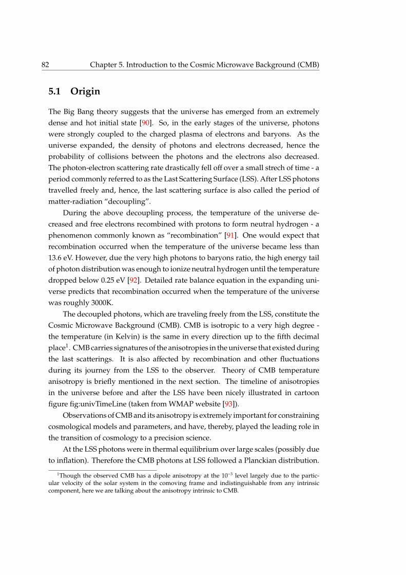
82 Chapter 5. Introduction to the Cosmic Microwave Background (CMB)
5.1 Origin
The Big Bang theory suggests that the universe has emerged from an extremelydense and hot initial state [90]. So, in the early stages of the universe, photonswere strongly coupled to the charged plasma of electrons and baryons. As theuniverse expanded, the density of photons and electrons decreased, hence theprobability of collisions between the photons and the electrons also decreased.The photon-electron scattering rate drastically fell off over a small strech of time - aperiod commonly referred to as the Last Scattering Surface (LSS). After LSS photonstravelled freely and, hence, the last scattering surface is also called the period ofmatter-radiation “decoupling”.
During the above decoupling process, the temperature of the universe de-creased and free electrons recombined with protons to form neutral hydrogen - aphenomenon commonly known as “recombination” [91]. One would expect thatrecombination occurred when the temperature of the universe became less than13.6 eV. However, due the very high photons to baryons ratio, the high energy tailof photon distribution was enough to ionize neutral hydrogen until the temperaturedropped below 0.25 eV [92]. Detailed rate balance equation in the expanding uni-verse predicts that recombination occurred when the temperature of the universewas roughly 3000K.
The decoupled photons, which are traveling freely from the LSS, constitute theCosmic Microwave Background (CMB). CMB is isotropic to a very high degree -the temperature (in Kelvin) is the same in every direction up to the fifth decimalplace1. CMB carries signatures of the anisotropies in the universe that existed duringthe last scatterings. It is also affected by recombination and other fluctuationsduring its journey from the LSS to the observer. Theory of CMB temperatureanisotropy is briefly mentioned in the next section. The timeline of anisotropiesin the universe before and after the LSS have been nicely illustrated in cartoonfigure fig:univTimeLine (taken from WMAP website [93]).
Observations of CMB and its anisotropy is extremely important for constrainingcosmological models and parameters, and have, thereby, played the leading role inthe transition of cosmology to a precision science.
At the LSS photons were in thermal equilibrium over large scales (possibly dueto inflation). Therefore the CMB photons at LSS followed a Planckian distribution.
1Though the observed CMB has a dipole anisotropy at the 10−3 level largely due to the partic-ular velocity of the solar system in the comoving frame and indistinguishable from any intrinsiccomponent, here we are talking about the anisotropy intrinsic to CMB.
5.1: Origin 83
Figure 5.1: Evolution of anisotropies in the universe. The timeline of differentanisotropies in the universe, including CMB at LSS, has been illustrated in thiscartoon. Image taken from the WMAP website [93].
Since the photons travelled freely after LSS, their distribution did not change. Thisfact was precisely established [94] by the Far Infrared Absolute Spectrophotometer(FIRAS) of the Cosmic Background Explorer (COBE) [95] satellite as shown infigure 5.2 (taken from the COBE website). The plot shows the theoretically expectedblackbody spectrum overlaid on the observed CMB frequency spectrum. The errorbars in the plot are hidden by the thickness of the line, showing the remarkablematch between theory and observation.
The expansion of the universe stretches the wavelengths of the CMB photonsand the density of the photons also decrease with the expansion. Therefore, thetemperature of the universe is inversely proportional to the scale factor; it can berelated to the cosmological redshift through the formula T(z) = (1 + z) T0, whereT0 is the observed temperature of the universe at redshift z = 0, the current epoch.From CMB observations we know that the temperature of the universe today is2.73K. Comparing this with the recombination temperature (∼ 3000K), one can seethat the LSS refers to a redshift of z ∼ 1100. According to the standard cosmologicalmodel, redshift of 1100 means ∼ 4 × 10⁵ years after the Big Bang. Thus, CMB is asnapshot of the universe when it was about 4 × 10⁵ years old.

84 Chapter 5. Introduction to the Cosmic Microwave Background (CMB)
Figure 5.2: Observed CMB frequency spectrum by COBE FIRAS. The spectrummatches the blackbody spectrum (Planckian) so remarkably well, that the theoreti-cally expected blackbody curve shown by the solid line, hides the (tiny) error barsin the plot. This image is taken from the COBE website [95].
5.2 CMB Anisotropy
The anisotropies in the CMB were originated from the primordial quantum fluctu-ations in the statistically homogeneous density field. These fluctuations had growndue to the gravitational instability and the corresponding anisotropy in the radia-tion density is imprinted on CMB as 10−5K fluctuations. The anisotropy of CMBtemperature field obtained from the three years’ data by the WMAP satellite hasbeen shown in figure 5.3. A polarization skymap has also been by made by fromthat data, which is overlaid on the temperature anisotropy map as solid lines. Theimage is taken from WMAP [93] press releases. See [96,97,98] for technical details.
These fluctuations are introduced in CMB through two mechanisms of redshiftvariations: anisotropy in gravitational redshift due to the anisotropy in gravitationalpotential ΦLSS(q) (Sachs-Wolf effect) and anisotropy in the redshift of scatteredphotons due to the anisotropy in the particular velocity of the LSS VLSS(q) inthe comoving frame (Doppler effect). The observed anisotropy in CMB is alsoaffected by the thickness of the last scattering surface ∆zLSS ∼ 80, which, in turn,is controlled by the process of recombination. The fluctuations at scales smallerthan the thickness of the last scattering surface are damped out. In the post-

5.2: CMB Anisotropy 85
Figure 5.3: WMAP CMB anisotropy sky. The 10−5K level temperature anisotropyskymap obtained from 3-years’ data of the WMAP satellite is shown in the figure.The polarization map obtained from that data is also overlaid on the map as solidlines. Image taken from WMAP [93] press releases. See [96, 97, 98] for technicaldetails.
recombination period, while CMB photons travel from the LSS to the observer, theymay cross anisotropic potential Φ(t, q) evolving with time and suffer a net redshiftthat introduces anisotropy in CMB (integrated Sachs-Wolf effect). Mathematically,we may write the observed CMB anisotropy ∆T(q) in a direction q as a fraction ofthe mean temperature T0 as [186]
∆T(q)T0
=
[q ·V(q)
c−
q ·VLSS(q)c
]+ΦLSS(q)
3c2 +2c2
∫∂∂tΦ(t, q) dt, (5.1)
where we have also considered the anisotropy introduced due to the particularvelocity of the solar system V(q) in the comoving cosmological frame.
The angular scale of the fluctuations at the LSS is mostly determined by thecompetition between the gravitational instability, which tries to increase anisotropyand radiation pressure, which tries to smooth density fluctuations. It can be shownthat this competition leads to what is known as the acoustic oscillations and theangular scale over which the patches on the LSS are correlated corresponds to theacoustic horizon at the LSS. The angular size of the acoustic horizon at the LSSas seen from the present epoch in a flat universe is ∼ 1. We shall explain in thenext section that CMB anisotropy is usually characterized by its angular powerspectrum. The peaks in the observed CMB power spectrum correspond to differentharmonics of the acoustic oscillation, where the first peak corresponds to an angular

86 Chapter 5. Introduction to the Cosmic Microwave Background (CMB)
size of ∼ 1.CMB also contains polarization anisotropy, which is usually classified into two
modes, E and B. The large scale anisotropy of B-mode polarization, generated bythe tensor perturbation in early universe, can be an important probe of inflation.CMB polarization has not been considered in the works presented in this thesis, seestandard references, e.g., [99], for a detailed introduction.
5.3 Angular Power Spectrum: Cosmic Variance
If CMB anisotropy is Gaussian, as predicted by well-accepted inflationary Big Bangmodel, the two point correlation function
C(q1, q2) := 〈∆T(q1)∆T(q2)〉, (5.2)
gives a complete description of the statistical properties of the anisotropy field.Further, if CMB anisotropy is statistically isotropic, the two point correlation functiondepends only on the angular separation between two directions, C(q1, q2) = C(q1 ·
q2), so it is quite convenient to expand it in a Fourier-Legendre series:
C(q1 · q2) =∞∑
l=0
2l + 14π
Cl Pl(q1 · q2), (5.3)
where Pl(x) is the Legendre polynomial of order l and Cl is the well known angu-lar power spectrum of CMB (anisotropy). The angular power spectrum of CMB(Cl) provides a complete description, equivalent to the two-point function, if CMBanisotropy is statistically isotropic and Gaussian. From analysis point of view,however, the angular power spectrum is preferred over the two point correlationfunction, because the power spectrum estimator Cl at different multipoles are uncor-related, at least, in case of a “perfect” CMB experiment which has full sky coveragewith circularly symmetric beam. In contrast, the two point correlation functions fordifferent angular separations are correlated.
Thus, the precise measurement of CMB anisotropy essentially means precisemeasurement of its angular power spectrum, which is one of the key challengesin experimental cosmology. To do so one first measures the spherical harmonictransform of the temperature anisotropy sky (over the 2-sphere):
alm :=∫
dΩq ∆T(q) Y∗lm(q). (5.4)

5.3: Angular Power Spectrum: Cosmic Variance 87
The statistical isotropy of the temperature anisotropy sky implies that
〈a∗lm al′m′〉 =
∫dΩq1
∫dΩq2 C(q1, q2) Ylm(q1) Y∗l′m′(q2) = Cl δll′ δmm′ , (5.5)
where we have made use of the addition theorem for the spherical harmonics [100]
4π2l + 1
l∑m=−l
Y∗lm(q1) Ylm(q2) = Pl(q1 · q2) (5.6)
and the orthogonality relation of the spherical harmonics∫dΩq Y∗lm(q) Yl′m′(q) = δll′ δmm′ . (5.7)
Therefore, to measure the CMB angular power spectrum, one can first computethe spherical harmonic transforms alm of the temperature anisotropy sky and then,according to the above relation, compute2
|alm|2, which is an unbiased estimator
of Cl. However, if the temperature anisotropy field is Gaussian, so is alm, hence|alm|
2 is χ2 distributed, therefore each measurement of |alm|2 will have certain error.
Since we have only one CMB sky, one can not reduce this error by taking multipleobservations. To reduce the error, we define the estimator for angular powerspectrum, Cl, by averaging over the independent “m” modes:
Cl :=1
2l + 1
l∑m=−l
|alm|2. (5.8)
Even then the estimated angular power spectrum will have certain error, which isindependent of the experimental precision. That is, even in an ideal CMB experi-ment, where we assume that the temperature in a certain direction can be measuredwith infinite precision, we can not measure the angular power spectrum with arbi-trary precision. The angular power spectrum estimated from the single realizationof the random CMB that can be observed leads to an inevitable uncertainty (akin tosample variance) known as the cosmic variance. For statistically isotropic Gaussian
2In practice, alm’s from two different frequency channels, which have independent noise, are cross-correlated to measure |alm|
2. This removes the noise bias, that is, makes the product of additive noiseterms from alm of zero mean and, hence, the estimator of Cl becomes unbiased.

88 Chapter 5. Introduction to the Cosmic Microwave Background (CMB)
CMB anisotropy, cosmic variance is given by
var(Cl) =2
2l + 1C2
l . (5.9)
The above formula for power spectrum estimator suggests that the “specific” cosmicvariance decreases with multipoles. Which is understandable as the number ofindependent “m” modes is more at high multipoles. Detailed derivation of theexpression for cosmic variance can be found in appendix C.
The best fit CMB power spectrum obtained from Wilkinson Microwave AnisotropyProbe (WMAP) [93] data compared to other experiments is shown in figure 5.4(taken from the LAMBDA website [101]). The first peak of the CMB power spec-
Figure 5.4: Observed CMB Power Spectrum. The best fit WMAP 3-year CMBpower spectrum is compared with the observed power spectrum from other recentexperiments. Note that the errors at the low multipoles and at the high Cl regionaround the first peak are cosmic variance dominated, this is the best any CMBexperiment can achieve at those multipoles given only one observable universe.Image taken from the LAMBDA website [101].
trum was located with extremely good accuracy by the WMAP experiment. Theerrors at the low multipoles and the high Cl region near the first peak are all cosmicvariance limited, which is the best any CMB experiment could achieve at thosemultipoles.
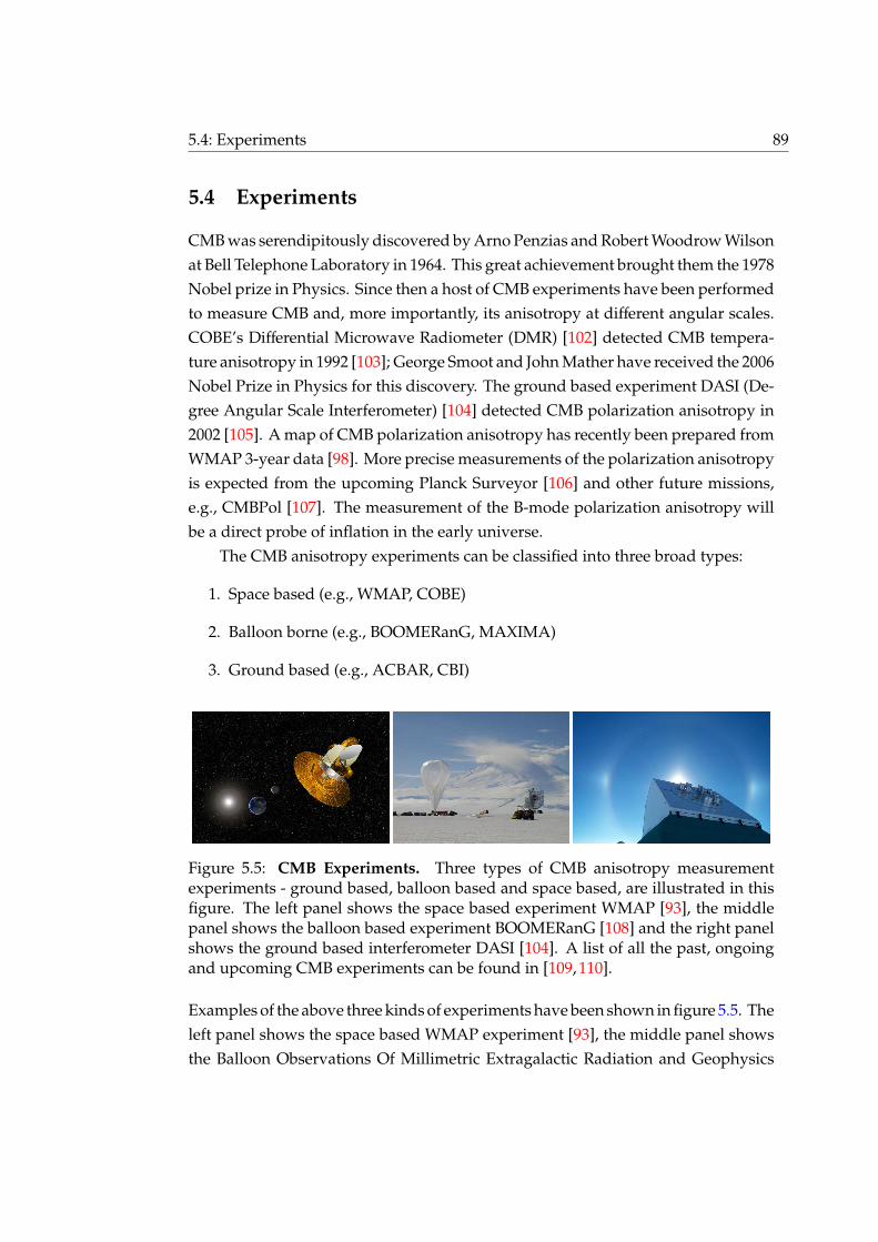
5.4: Experiments 89
5.4 Experiments
CMB was serendipitously discovered by Arno Penzias and Robert Woodrow Wilsonat Bell Telephone Laboratory in 1964. This great achievement brought them the 1978Nobel prize in Physics. Since then a host of CMB experiments have been performedto measure CMB and, more importantly, its anisotropy at different angular scales.COBE’s Differential Microwave Radiometer (DMR) [102] detected CMB tempera-ture anisotropy in 1992 [103]; George Smoot and John Mather have received the 2006Nobel Prize in Physics for this discovery. The ground based experiment DASI (De-gree Angular Scale Interferometer) [104] detected CMB polarization anisotropy in2002 [105]. A map of CMB polarization anisotropy has recently been prepared fromWMAP 3-year data [98]. More precise measurements of the polarization anisotropyis expected from the upcoming Planck Surveyor [106] and other future missions,e.g., CMBPol [107]. The measurement of the B-mode polarization anisotropy willbe a direct probe of inflation in the early universe.
The CMB anisotropy experiments can be classified into three broad types:
1. Space based (e.g., WMAP, COBE)
2. Balloon borne (e.g., BOOMERanG, MAXIMA)
3. Ground based (e.g., ACBAR, CBI)
Figure 5.5: CMB Experiments. Three types of CMB anisotropy measurementexperiments - ground based, balloon based and space based, are illustrated in thisfigure. The left panel shows the space based experiment WMAP [93], the middlepanel shows the balloon based experiment BOOMERanG [108] and the right panelshows the ground based interferometer DASI [104]. A list of all the past, ongoingand upcoming CMB experiments can be found in [109, 110].
Examples of the above three kinds of experiments have been shown in figure 5.5. Theleft panel shows the space based WMAP experiment [93], the middle panel showsthe Balloon Observations Of Millimetric Extragalactic Radiation and Geophysics

90 Chapter 5. Introduction to the Cosmic Microwave Background (CMB)
(BOOMERanG) experiment [108] and the right panel shows the ground based DASIinstrument [104]. A list of past, ongoing and future CMB experiments can be foundin, e.g., [109, 110]. The timeline of CMB astronomy is listed at [111]. The detailsof the instrumentation in CMB experiments is beyond the scope of this thesis.Specific details about the instruments, in particular, about the WMAP satellite, willbe provided wherever necessary.
5.5 Summary and Conclusion
According to the widely accepted working Big bang model of the history of theuniverse, the universe was a very hot and dense soup of photons and chargedplasma. As the universe expanded, its density and temperature of reduced andphotons started traveling freely. The electrons and protons also recombined duringthis time, known as the Last Scattering Surface (LSS). The anisotropies at the LSSare embedded as tiny fluctuations in the CMB. Measurement of these fluctuationsare extremely important for constraining cosmological models and parameters andhas played a leading role in the transition of cosmology to a precision science.
Standard Big Bang model also predicts that the CMB anisotropy is Gaussian andwe observe that the universe is highly isotropic. Because of that, CMB anisotropyis usually characterized by the angular power spectrum, as it provides a completestatistical description of a statistically isotropic Gaussian random field on a 2-sphere.Precise measurement of CMB anisotropy is then equivalent to precise measurementof position and height of the crests and troughs of the CMB power spectrum.
CMB was serendipitously discovered by Penzias and Wilson in 1964 and CMBanisotropy was first detected by COBE in 1992. Since then several space based,balloon borne and ground based experiments have been performed to preciselymeasure the CMB power spectrum at different scales. The first peak of the CMBtemperature power spectrum was precisely determined by the WMAP satellite.Its 3-year data has also provided a CMB polarization anisotropy map, which wasfirst detected by DASI in 2002. Detection of the B-mode polarization due to tensorperturbation in the early universe will be a direct probe of inflation.
The precision of these highly sensitive experiments can be properly utilized ifall the significant systematic effects are removed. Study of the systematic effects inCMB experiments, in particular, the WMAP satellite, is one of the major goals ofthis thesis.
91
Chapter 6
Beams and Deconvolution inCMB and GWB Mapmaking:Analysis and Formalism
The observed skymaps of CMB and GWB are convolved with a beam function, a. k.a., the Point Spread Function (PSF). The observed skymaps need to be deconvolvedfor the estimation of the true skymaps.
The beam function of a CMB instrument is combined with the scan strategyof the instrument and presented as a mapping matrix. The observed time ordereddata is a convolution of the mapping matrix with the true sky map. On the otherhand, the (directed) GW radiometer beam patterns are extended, quite asymmetricand vary with sky position. We present an analytical study of the GW radiometerbeam involving stationary phase approximation to explain the shape of the beam.Also, unlike CMB map making, the GW radiometer analysis is in a preliminarystage. The definition of beam function and the observed data in CMB and GWBexperiments are discussed respectively in section 6.1, section 6.2 and section 6.3.
The observed quantities in both CMB and GWB analysis can be expressed asa linear convolution equation. Because of the broad overlap between the kindof map estimation problem we are addressing in CMB and GWB, it is expectedthat similar techniques will be applicable to both analyses. CMB map makingtechniques are quite mature and have been tested for a long time. So, to begin with,we essentially follow the prescription based on maximum likelihood estimationfollowed in CMB analysis. The analytical details of maximum likelihood mapmaking and its application to CMB and GWB analysis are presented in section 6.4,

92Chapter 6. Beams and Deconvolution in CMB and GWB Mapmaking:
Analysis and Formalism
section 6.5 and section 6.6 respectively.
Though the analysis that has been used here for GWB map making, was firstdeveloped for CMB analysis, it can not be implemented with full strength to makeCMB maps using modern high-resolution instruments for the following reason: TheCMB beams are mildly non-circular and this systematic effect has to be correctedfor high resolution experiments. But incorporating this in a maximum likelihoodanalysis is computationally prohibitive. A suboptimal analysis to correct for beamanisotropy in CMB analysis has been developed in chapter 8 and chapter 9.
6.1 Beam Function
Due to the finite resolution of imaging devices, a point source is mapped to an imageof finite size. Similarly when the device is pointed to a certain direction, it receivescontributions from the neighboring directions also. The function that describes theimage of a point source or the response function of the device for each direction isknown as the beam function or the point spread function (PSF) or the kernel. Thebeam function B(Ω, Ω′) is the observed effect in the direction Ω due to a unit pointsource in the direction Ω′; it is, in fact, the kernel of the convolution equation. Forpractical purposes the sky is pixelized and the beam function is represented by amatrix. The beam function (or the matrix) can be interpreted in two ways:
1. B(Ω, Ω′) is the response function for the pointing direction Ω(each column of the beam matrix is a response function)
2. B(Ω, Ω′) is the point spread function for the source direction Ω′
(each row of the beam matrix is a point spread function)
Usually a beam function is maximum along the direction where the device is point-ing; it falls off (often rapidly) as the distance between the image point and thepointing direction increases. The size of the beam is quantified by its Full Width atHalf Maximum (FWHM). In many imaging devices there are secondary peaks alsoin the beam functions, which are known as “side lobes”.
6.2 Observed CMB Data
Several experiments have been performed to measure CMB anisotropy at differentangular scales. Most of the CMB experiments have beams of fairly axisymmetric

6.2: Observed CMB Data 93
shape, which can be approximated by two dimensional Gaussian functions. WMAPanalysis is of particular concern in this thesis. We have shown the WMAP beampatterns below and we have fitted WMAP Q-beam in appendix D using the IRAFimage processing software. See chapter 8, chapter 9 and appendix D for details.
The goal of the WMAP mission is to make skymaps of CMB anisotropy. TheWMAP satellite spins in space and scans the whole sky in this process. At each ob-servation time the horns A and B of the instruments point in two different directionsand the difference in temperature detected by the two horns is measured. So, giventhe scan strategy, the observation time can be mapped to pointing direction of eachhorn. At any given moment, though each horn points in a certain direction, due tothe finite resolution of the instruments, photons are received from its neighboringdirections as well. The beam function describes the fractional energy received fromeach direction corresponding to a certain pointing direction.
In modern astronomical experiments, often an imaging device is capable ofcreating more than one image of a point source on the focal plane for differentparameters, e.g, polarization, frequency bands. Figure 6.1 shows the temperaturebeam maps of the two horns of the WMAP satellite. Each image plane (side A andB) shows the images of Jupiter (treated as a point source) for 10 frequency channelsused for observing CMB anisotropy. Jupiter was observed during different seasonsto account for the variation in apparent shape due to different observation angles.The sizes of the WMAP beams vary from 0.22 to 0.88. The shape of the WMAPbeams do not vary with sky position, which is a very important property and willbe of great use later on.
In a practical application we need to pixelize the sky. Each pixel is given aunique number, so effectively the two dimensional sky can be represented by onepixel index - a skymap can be expressed by a real vector. Thus the combined effectof the scan strategy and the beam function for each horn can be represented by amapping matrix MA,B
≡ MA,Bij . Each row of the mapping matrix corresponds to a
certain observation time. Elements of each row of the mapping matrix is a beampattern function for the pointing direction corresponding to that observation time.At every observation time, the instrument measures the difference between thetemperature anisotropies between two horn pointing directions; the full observationtime generates a vector of Time Ordered Data (TOD) d. For a differential instrumentlike WMAP, the mapping matrix M ≡Mi j, that convolves the true map to generate

94Chapter 6. Beams and Deconvolution in CMB and GWB Mapmaking:
Analysis and Formalism
Figure 6.1: WMAP image planes. The image of Jupiter (as a point source) indifferent frequency bands taken by two horns of the WMAP satellite. (Images takenfrom the LAMBDA website [101]).
the final output, is the difference between the mapping matrices of two horns [96]
M = MA−MB. (6.1)
For computational simplicity to be explained later, the beam functions of each hornare assumed to be of infinite resolution and circular (axially symmetric about thepointing direction). So one element of each row of the pointing matrices MA,B is 1at the pixel (column) index that corresponds to the pointing direction at the giventime (row index). All other elements of the matrices are 0.
Since the true temperature anisotropy map t is independent of time, one maywrite the observed CMB time ordered data as the convolution equation
d = M · t + n (6.2)
where n is the random instrumental noise. WMAP noise is nearly white zero meanGaussian, so the noise covariance matrix [96] is given by
N := 〈n nT〉 = σ2
0 I, (6.3)
where σ20 is the variance of each bin of time ordered data and I is the identity matrix.
Thus the measured time ordered data d from a CMB anisotropy experiment is

6.3: Observed (Directed) GW Radiometer Point Estimate 95
a convolution of the true sky t with the known mapping matrix M and has additivenoise n of known statistical properties. In the next section we shall see that theoutput of the GW radiometer can also be expressed in a similar fashion as a linearconvolution equation. We then present a general deconvolution method applicableto both CMB and GWB for the estimation of the true anisotropy sky.
6.3 Observed (Directed) GW Radiometer Point Estimate
As described in section 4.4.2, it is possible to make a skymap using a directed GWradiometer. The detailed properties of the beam function and convolution equationof the radiometer is presented in this section. From now on we shall only considerthe issues of map making using a directed GW radiometer, so the tag “directed” isimplied and hence will be omitted.
A GW radiometer is pointed to a direction Ω by using a direction dependentfilter function
qΩ,H(t, f ) =H( f )γ∗
Ω(t, f )
P1(t; | f |) P2(t; | f |). (6.4)
Suppose that there is only one unit polarized point source in the sky in the directionΩ′, that is PA
true(Ω) = δAA′δ(Ω − Ω′). Then the expected point estimate (statistic)SΩ is maximum when Ω = Ω′ and it falls of as the distance between the pointingdirection and the source direction, ∆Ω := Ω − Ω′, increases, when Ω is close to Ω′.The expected point estimate 〈SΩ〉 in this case is the polarization dependent beamfunction BA(Ω, Ω′) for the GW radiometer. Formally, we can express the beamfunction using eqn (4.88) and eqn (4.98) as
BA(Ω, Ω′) =
∆tn∑
i=1
‖qΩ,H‖2ti
−1
∆tn∑
i=1
∫∞
−∞
d f Htrue( f )γAΩ′
(ti, f ) qΩ,H(ti, f ) (6.5)
=
∆tn∑
i=1
‖qΩ,H‖2ti
−1
∆tn∑
i=1
∫∞
−∞
d fHtrue( f ) H( f )
P1(ti; | f |) P2(ti; | f |)γAΩ′
(ti, f )γ∗Ω
(ti, f ).
(6.6)
Using the polarization and direction dependent overlap reduction function
γAΩ
(t, f ) := FA1 (Ω, t) FA
2 (Ω, t) e2πi f Ω·∆x(t)/c, (6.7)

96Chapter 6. Beams and Deconvolution in CMB and GWB Mapmaking:
Analysis and Formalism
the shorthands for the combination of the antenna pattern functions
Γ(Ω, t) := F+1 (Ω, t) F+2 (Ω, t) + F×1 (Ω, t) F×2 (Ω, t) (6.8)
and representing the ratio of source and noise PSDs through a single function
G(t; f ) :=Htrue( f ) H( f )
P1(t; | f |) P2(t; | f |), (6.9)
the beam function can be expressed in a more compact form
BA(Ω, Ω′) =
∆tn∑
i=1
‖qΩ,H‖2ti
−1
×
∆tn∑
i=1
∫∞
−∞
d f G(ti; f )FA1 (Ω′, ti)FA
2 (Ω′, ti)Γ(Ω, ti)e−2πi f∆Ω·∆x(ti)/c.(6.10)
If the detector noise PSDs are stationary, the shape of the beam functions for integra-tion over complete day(s) do not depend on the longitude of the pointing directiondue to the symmetry about earth’s spin axis.
If the injected unit point source is unpolarized, we may useP+true(Ω) = P×true(Ω) =δ(Ω − Ω′) and the polarization independent beam functions becomes
B(Ω, Ω′) = B+(Ω, Ω′) + B×(Ω, Ω′) (6.11)
=
∆tn∑
i=1
‖qΩ,H‖2ti
−1
∆tn∑
i=1
∫∞
−∞
d f G(ti; f )Γ(Ω′, ti)Γ(Ω, ti) e−2πi f∆Ω·∆x(ti)/c.
(6.12)
From now on we shall assume that the true source PSD is exactly known, Htrue( f ) =H( f ), unless otherwise specified (so we omit the subscript “H” from the filter). Withthis assumption, it is interesting to note that
B(Ω, Ω′) =
∆tn∑
i=1
(qΩ, qΩ′)
/∆t
n∑i=1
‖qΩ‖2ti
, (6.13)
which follows the convenient normalization condition B(Ω, Ω) = 1 [see eqn (4.79)].
Typical (polarization independent) beam functions for the baseline formed bythe two LIGO detectors at Hanford and Livingston (for white noise PSD with uppercutoff frequency 1024Hz and observation over a full day) are shown in the left panel

6.3: Observed (Directed) GW Radiometer Point Estimate 97
of figure 6.2.
Figure 6.2: Numerical and Theoretical GW radiometer beam patterns. The leftpanel shows a numerical beam patterns for the LIGO Hanford-Livingston base-line pointing at latitude 12 for white noise with an upper cut-off frequency of1024Hz. The right panel shows the theoretical pattern obtained by stationary phaseapproximation (SPA). Clearly they are in very good agreement.
The size of the beam of the radiometer using the LIGO Livingston and Hanforddetectors can vary between∼ 50−100 sq. degrees [79] depending on the sky position,the upper cutoff frequency and the source and noise PSDs. Typical contour plots ofthe beam function including the (negative) side lobes of the LLO-LHO radiometernear latitude 12 for LIGO-I noise PSD and different source PSDs are shown infigure 6.3. The source PSD for the left panel is H( f ) = constant and for the rightpanel is H( f ) ∝ f−3.
The GW radiometer beams have quite asymmetric shape and they vary with skyposition. This compelled us to understand the characteristic of the beam function.In appendix B we have analytically studied the beam pattern using StationaryPhase Approximation (SPA). Where we have used the fact that the functions G(t; f )and Γ(Ω, t) are slowly varying functions of time, so the integrand constructivelycontributes when the phase term exp[−2πi f∆Ω · ∆x(t)/c] is stationary. We showthat the beam function B(Ω, Ω0) for a pointing direction Ω0 takes significant valueswhen Ω − Ω0 is parallel to the unit normal ncone(t) to the baseline vector ∆x(t) andthe cone traced out by the baseline due to earth rotation. Mathematically, the beampattern stands out along the following trajectory parameterized by sideral time t:
Ω(t) = Ω0 − 2 [Ω0 · ncone(t)] ncone(t). (6.14)

98Chapter 6. Beams and Deconvolution in CMB and GWB Mapmaking:
Analysis and Formalism
Figure 6.3: Contour plots of GW radiometer beam patterns. Approximate size ofthe beam and the (negative) side lobes for different source PSDs and LIGO detectorswith LIGO-I noise PSD are shown in this figure. The left panel shows the beamcontours for H( f ) = constant at latitute 12 and the right panel shows the same forH( f ) ∝ f−3. The contours are drawn starting from 1 with an interval of −0.1. Notethat, the beam falls by 1/e in between the 6th and the 7th contour (from the highestvalue), which can be used to measure the beam size.
The theoretical pattern is shown in the right panel of figure 6.2, which is in verygood agreement with the numerical pattern shown in the left panel.
We proceed further and evaluate the (unnormalized) beam function along thistrajectory using the formula, again parameterized with time t
B(Ω(t), Ω0) ∝ Γ(Ω(t); t)Γ(Ω0; t)
√fu −
√fl
ωE
√8 c∣∣∣[z · ∆x(t)] [z · (Ω(t) − Ω0)]
∣∣∣ , (6.15)
where fl and fu are respectively the lower and upper cutoff frequencies.
The stationary phase analysis also indicates an approximate resolving powerof the radiometer. The expression for the phase term 2πi f∆Ω ·∆x(t)/c suggests thatthe resolving power of the radiometer is ∼ c/ fu/∆R, where λ corresponding to theupper cutoff frequency fu. For the LIGO detectors separated by ∼ 3000km with aupper cut off frequency of fu ∼ 1kHz (wavelength ∼ 300km). Hence the radiometerresolution should be ∼ 0.1 radians, that is, ∼ 6 degrees, which is consistent with thenumerically obtained beam profiles.
In general, the true sky is a diffuse background of stochastic GW. If the trueangular power distribution is described by the polarization dependent functionP
Atrue(Ω), it is straight forward to show using eqn (4.88) that the observed point
estimate SΩ is a convolution of the the true sky PAtrue(Ω) with the known beam
6.3: Observed (Directed) GW Radiometer Point Estimate 99
function BA(Ω, Ω′) and has additive noise nΩ of known statistical properties:
SΩ =∫
S2dΩ′
[B+(Ω, Ω′)P+true(Ω′) + B×(Ω, Ω′)P×true(Ω′)
]+ nΩ. (6.16)
Notice the similarity with the CMB time-ordered-data described in the previoussection. Our aim is to estimate the true angular power distribution PA
true(Ω) fromthe above integral equation. To be able to do that, we need to study the statisticalproperties of noise at each pixel.
Unlike CMB, the GW radiometer noise is quite complicated. The noise atdifferent pixel (direction) is related to the detector time stream data through theradiometer analysis, hence, the noise nΩ at different directions are correlated. Thestatistical properties of the noise nΩ are given below.
The noise term in the radiometer signal will have terms containing summationsover nI nJ and hI nJ, where I, J = 1, 2 are the detector indices. All these terms are ofzero mean for I , J, but the variance will be highly dominated by the noise-noiseterm [〈n∗I nI〉 〈h∗J hJ〉]. Hence, while considering the noise characteristics the otherterms are ignored. Moreover, the noises in the detectors are independent, whichimplies that [112], for I , J, 〈n∗I nJ〉 = 〈n∗I〉〈nJ〉 and 〈n∗I n
∗
I nJnJ〉 = 〈n∗I n∗
I〉〈nJnJ〉.
• Noise in point estimate:
nΩ =
∆tn∑
i=1
‖qΩ‖2ti
−1 n∑
i=1
∫∞
−∞
d f n∗1(ti; f ) n2(ti; f ) qΩ(ti, f ). (6.17)
• Mean of noise:
〈nΩ〉 =
∆tn∑
i=1
‖qΩ‖2ti
−1 n∑
i=1
∫∞
−∞
d f 〈n∗1(ti; f )〉〈n2(ti; f )〉 qΩ(ti, f ) = 0. (6.18)

100Chapter 6. Beams and Deconvolution in CMB and GWB Mapmaking:
Analysis and Formalism
• Pixel-to-pixel covariance of observed noise :
〈nΩ1nΩ2〉 =
∆tn∑
i=1
‖qΩ1‖
2ti
−1 ∆t
n∑i=1
‖qΩ2‖
2ti
−1 n∑
i1=1
n∑i2=1∫
∞
−∞
d f1
∫∞
−∞
d f2
∫∞
−∞
d f ′1
∫∞
−∞
d f ′2 δ∆t( f1 − f ′1) δ∆t( f2 − f ′2) ×
〈n∗1(ti1 ; f1)n∗1(ti2 ; f2)〉〈n2(ti1 ; f ′1 )n2(ti2 ; f ′2)〉 qΩ1(ti1 , f ′1) qΩ2
(ti2 , f ′2)
=14
∆tn∑
i=1
‖qΩ1‖
2ti
−1 ∆t
n∑i=1
‖qΩ2‖
2ti
−1 n∑
i=1
∫∞
−∞
d f1
∫∞
−∞
d f ′1
δ2∆t( f1 − f ′1) P1(ti, | f1|) P2(ti, | f ′1 |) qΩ1
(ti, f ′1) q∗Ω2
(ti, f ′1)
=∆t4
∆tn∑
i=1
‖qΩ1‖
2ti
−1 ∆t
n∑i=1
‖qΩ2‖
2ti
−1
×
n∑i=1
∫∞
−∞
d f P1(ti, | f |) P2(ti, | f |) qΩ1(ti, f ) q∗
Ω2(ti, f ). (6.19)
The covariance can be expressed in a convenient form using eqn (6.13)
〈nΩ1nΩ2〉 =
14
∆tn∑
i=1
‖qΩ2‖
2ti
−1
B(Ω1, Ω2) =14
∆t∑n
i=1(qΩ1, qΩ2
)
∆t∑n
i=1‖qΩ1‖2ti∆t
∑ni=1‖qΩ2
‖2ti
.
(6.20)
• Noise variance [see eqn (4.82)]
〈nΩ nΩ〉 =14
∆tn∑
i=1
‖qΩ‖2ti
−1
. (6.21)
The covariance formula gives the same consistent result for Ω1 = Ω2 = Ω.
Moreover, the probability distribution of the noise n(Ω) is normal (so the firstand the second moments characterize all the statistical properties). This is ensuredby the generalized central limit theorem [113]: If Xk be mutually independent onedimensional random variables following distributions Fk with mean 0 and varianceσ2
k , then∑
k Xk tend to follow a zero mean normal distribution with variance∑
k σ2k .
Since several realizations of the products of Fourier transforms of detector noisen∗1(t; f ) n2(t; f ) are added [see eqn (6.17)] to generate the noise n(Ω), the generalizedcentral limit theorem suggests it may be Normal distributed. As a consistency

6.4: Maximum Likelihood (ML) skymap Estimation 101
check, if this argument is used to calculate the variance of n(Ω), we get the sameresult as in eqn (6.21).
For practical applications, the sky is pixelized and the true power distributionis usually expanded as a sum of point sources at each pixel,
PAtrue(Ω) =
∑k
PAk δ(Ω − Ωk), (6.22)
where Ωk is the location of pixel k and PAk is the strength of pixel k. Then, we may
write the discrete convolution equation as
S = B+ ·P+ + B× ·P× + n, (6.23)
where the indices of the vectors and matrices in the above equation refers to thecorresponding pixel, more explicitly, Bkk′ ≡ B(Ωk, Ωk′), Sk ≡ SΩk
and nk ≡ nΩk. The
pixel to pixel noise covariance matrix in the observed map N ≡ Nkk′ becomes
Nkk′ := 〈nk nk′〉 =14
∆tn∑
i=1
‖qΩk′‖
2ti
−1
Bkk′ . (6.24)
The convolution equation for GWB point estimates [eqn (6.23)] is strikingly sim-ilar to the convolution equation for the CMB time-ordered-data given by eqn (6.2).Therefore, in effect, the problem of estimation of true GWB anisotropy map from thepoint estimate at every pixel is identical to the estimation of true CMB anisotropymap from the time-ordered-data. The procedure to estimate the maximum likeli-hood skymap is described in the next section.
6.4 Maximum Likelihood (ML) skymap Estimation
In the last two sections we have established that the CMB and GWB observed mapcan be expressed by a linear convolution equation of the form
d = K · t + n, (6.25)
where our aim is to estimate the true sky vector t from the observed data vector dusing the known kernel matrix K and the known statistical properties of the Gaussiannoise vector n. This problem has been addressed in different branches of scienceusing different approaches. Since CMB map making has been developed and

102Chapter 6. Beams and Deconvolution in CMB and GWB Mapmaking:
Analysis and Formalism
successfully implemented for more than a decade, we opt for the algorithm usedfor CMB anisotropy map making [114]. This algorithm estimates the MaximumLikelihood (ML) solution from a linear convolution equation with Gaussian noise,which was put together by Borrill [115] as a (publicly available) software packageMADCAP [116]. The same algorithm was used to make anisotropy maps using therecently released data from the WMAP satellite [97].
The mathematics is straight forward. If noise follows a multivariate normaldistribution, the probability that the data contains the noise vector n is given by [112]
P(n) =1
(2π)Nd/2(det N)1/2exp
[−
12
nT·N−1
· n]
(6.26)
where Nd is the number of observed data points (number of elements in d), N :=〈n nT
〉 is the (symmetric) noise covariance matrix of the observed data and det N isthe determinant of N. Therefore the probability (likelihood) that the data d containsthe modeled signal tmod is
P(d|tmod) = (2π)−Nd/2 exp[−
12
((d −K · tmod)T
·N−1· (d −K · tmod) + Tr[ln N]
)].
(6.27)The corresponding log-likelihood is
ln[P(d|tmod)] = −12
((d −K · tmod)T
·N−1· (d −K · tmod) + Tr[ln N]
)+
Nd
2ln(2π).
(6.28)It can be shown by taking derivative of the above equation with respect to tmod [112]that the (log-)likelihood is maximum when
tmod =(KT N−1 K
)−1KT N−1
· d =: t, (6.29)
which is the maximum likelihood estimate for the given problem. For clarity, weshall use the short hand
W :=(KT N−1 K
)−1KT N−1. (6.30)
It is important to note that WK = I, where I is the identity matrix. Hence,
t = W · d = W · (K · t + n) = t + W · n. (6.31)
Since the noise in observed data is of zero mean, 〈n〉 = 0, the above relation suggests
6.5: ML Estimation of CMB Anisotropy Map 103
that the ML estimate is unbiased: 〈t〉 = t.The noise in the ML estimate n is a convolution of the noise n in observed data
with the matrix W:n := t − 〈t〉 = t − t = W · n. (6.32)
The noise covariance matrix of the ML estimate is
Σ := 〈nnT〉 = W 〈nnT
〉WT =(KT N−1 K
)−1KT WT =
(KT N−1 K
)−1. (6.33)
Therefore, to obtain the ML estimate one has to first compute the inverse of thenoise covariance matrix Σ−1 = KTN−1K, then invert it to evaluate W and, in turn, t.
6.5 ML Estimation of CMB Anisotropy Map
The above mathematics is directly applicable to CMB map making. The ML estimateof the true temperature anisotropy map is given by
t = W · d; W =(MT N−1 M
)−1MT N−1. (6.34)
The pixel-to-pixel noise covariance matrix of the estimated map is
Σ =(MT N−1 M
)−1. (6.35)
However, in practice, the solution t = W · d is too costly to evaluate exactlygiven the properties of M and N−1 [96]. This is mainly due to very high resolu-tions of modern CMB experiments and correspondingly large sizes of the matrices.Approximate techniques are adopted for the implementation of the ML analysis.For example, in the map making carried out by the WMAP team, the beams areassumed to be circularly symmetric (about the pointing direction) with infinite res-olution for the evaluation of the matrix W and the above analysis is then used toestimate the true anisotropy map.1 Though this assumption is approximately validfor preparing sky maps, it introduces a bias in the skymap and angular power spec-trum [117, 118]. This systematic effect is quite significant at high multipoles (lowangular scales beyond the beam width), and has to be considered for correct dataanalysis. Different approaches to deconvolve partial or full skymap for asymmetricbeams are being proposed [119,120]. We have developed a sub-optimal approach to
1Similar formalism has been used to make CMB polarization anisotropy map also using the threeyears of WMAP data [96, 98].

104Chapter 6. Beams and Deconvolution in CMB and GWB Mapmaking:
Analysis and Formalism
unbias the (pseudo-Cl) power spectrum estimator, which is presented in chapter 8and chapter 9. The effect of beam asymmetry has been taken into account in therecent WMAP three years analysis [96] using a similar approach; the results are invery good agreement with our prediction.
6.6 ML Estimation of GWB Anisotropy
A straightforward application of ML estimation method described in the previoussection to GWB skymap making is presented in this section. While we first presentthe simplest case of a sigle baseline interferometry, It is possible to extend the basicanalysis to incorporate more complex problems of using multiple baselines and/ormaking separate maps for each polarization and to measure multipole moments ofthe GWB sky.
6.6.1 Basic Analysis of Skymap
We shall first consider the case of single baseline with equal power in both polar-izations, P+(Ω) = P×(Ω). The ML estimate for the GWB sky map is given by
P = W · S; W =(BT N−1 B
)−1BT N−1 (6.36)
and the pixel-to-pixel noise covariance matrix of the observed map is
Σ =(BT N−1 B
)−1. (6.37)
Since in this special case the beam matrix is a square matrix, if the inverse of thebeam matrix exists the ML estimate takes a simple form
P = B−1· S. (6.38)
However directly inverting the beam matrix is non-trivial and we prefer to solvethe following linear algebraic equation to find P:
B · P = S. (6.39)
This issue will be illustrated in the next section.It is worth noting that in the case of GWB map making a full blown ML estimate
can be implemented because, as compared to the modern CMB experiments, GW

6.6: ML Estimation of GWB Anisotropy 105
radiometer beam for the ground based detectors is much broader, so the number ofpixels (and hence the dimension of the matrices) is numerically tractable.
6.6.2 Extensions of the simple MapMaking
The ML analysis to estimate the GWB skymaps can be generalized to address morecomplex problems of using a network of detectors (multiple baselines) and makingseparate maps for different polarizations. In each case the form of the expressionsfor the ML estimate (P) and pixel-to-pixel covariance matrix (Σ) remain the same,
P = ΣBT N−1· S; Σ−1 := BTN−1B, (6.40)
as long as the form of the convolution equation,
S = B ·P + n, (6.41)
is preserved by redefining different quantities in that equation.
Network of Detectors
The description of GWB radiometer beam and its convolution provided in sec-tion 6.3 only considered the problem of map making using one baseline (two detec-tors). However, if we have observed maps (with same pixelization) from differentbaselines of a network of detectors, we have to incorporate all the baselines byredefining different quantities to get the ML estimate.2
Suppose that Nb baselines have generated skymaps of identical pixelizationwith Npix pixels. Let S(i) be the observed map by baseline i, mapped using the filter“vector” q(i), convolved with beam matrix B(i) and contains noise n(i). Then the
2Of course, one could also combine the maps from different baselines with suitable pixel dependentweight factors wi,
S =∑
i
wi · S(i),
which may reduce the noise by a factor of ∼√
Nb. But, it would also have issues of combining datafrom baselines with different beam functions. Further analysis is required to assess which methodwould be more advantageous.

106Chapter 6. Beams and Deconvolution in CMB and GWB Mapmaking:
Analysis and Formalism
form of the convolution equation [eqn (6.41)] can be preserved by substituting
S :=
S(1)
S(2)
...
S(Nb)
; n :=
n(1)
n(2)
...
n(Nb)
; B :=
B(1)
B(2)
...
B(Nb)
. (6.42)
Note that S, n are now 1 × NpixNb vectors and B is a Npix × NpixNb matrix, whileP (the true GWB sky) remains unchanged. This is similar to CMB experimentswhere each pixel is visited by the detector several times. In the multi-baseline GWradiometer case each pixel is visited by different baselines, but, unlike CMB, eachpixel is visited equal number of times. The noise covariance matrix N := 〈nnT
〉 ofthe raw skymap should also be generalized. Let n(i)
Ωbe the noise from the radiometer
baseline i with detectors I and I′ (and following the same convention for j) pointingat Ω. Then
〈n(i)Ω1
n( j)Ω2〉 =
∆tn∑
i1=1
‖q(i)Ω1‖
2ti1
−1 ∆t
n∑i2=1
‖q( j)Ω1‖
2ti2
−1 n∑
i1=1
n∑i2=1∫
∞
−∞
d f1
∫∞
−∞
d f2
∫∞
−∞
d f ′1
∫∞
−∞
d f ′2 δ∆t( f1 − f ′1) δ∆t( f2 − f ′2) ×
〈n∗I(ti1 , f1)n∗J(ti2 , f2)nI′(ti1 , f ′1 )nJ′(ti2 , f ′2)〉 q(i)Ω1
(ti1 , f ′1) q( j)Ω2
(ti2 , f ′2).
(6.43)
If i and j denote the same baselines we get back the covariance for single baseline[eqn (6.19)]. However, if i and j denote different baselines, at least one pair of thedetectors among the two pairs will be different (i.e., either I , J or I′ , J′), so inthat case 〈n(i)
Ω1n( j)Ω2〉 = 0. Hence the matrix N will be a block diagonal matrix, with
diagonal elements N(i) := 〈n(i)n(i)T〉 - the covariance matrix of baseline i.
Polarization Maps
We may even make skymaps for different polarizations separately by generalizingthe definitions of different quantities in the ML analysis. The discrete convolutionequation
S = B+ ·P+ + B× ·P× + n (6.44)

6.6: ML Estimation of GWB Anisotropy 107
can also be expressed as eqn (6.41) by substituting
B :=[
B+ B×]
; P :=
P+P×
. (6.45)
Polarization Maps using a Network of Detectors
Finally, we may combine the previous two generalizations to estimate maps for eachpolarization separately using multiple baselines. We use the generalized definitionsof P given in eqn (6.45) containing the two polarization map vectors and signal Sand noise n corresponding to multiple baselines given by eqn (6.42). We thengeneralize the definition of beam matrix B even more by putting
B :=
B(1)+ B(1)
×
B(2)+ B(2)
×
......
B(Nb)+ B(Nb)
×
, (6.46)
which now combines the effect of each individual baseline and polarization.
6.6.3 Multipole moments from the directed search
The convolution equation:
〈S(Ω)〉 =∫
S2dΩ′ B(Ω, Ω′)Ptrue(Ω′). (6.47)
The angular power distribution can be expanded in terms of spherical harmonics,
Ptrue(Ω) =∑lm
Plm Ylm(Ω) (6.48)
B(Ω, Ω′) =∑lm
Blm(Ω) Ylm(Ω), (6.49)
and substituted the above in the convolution equation:
〈S(Ω)〉 =∑lm
Plm
∫S2
dΩ′ B(Ω, Ω′) Ylm(Ω′) =∑lm
PlmB∗lm(Ω). (6.50)
108Chapter 6. Beams and Deconvolution in CMB and GWB Mapmaking:
Analysis and Formalism
The spherical harmonic transform of the convolution equation
〈Sl′m′〉 :=∫
S2dΩ 〈S(Ω)〉Y∗l′m′(Ω) =
∑lm
Plm
∫S2
dΩB∗lm(Ω)Y∗l′m′(Ω) =∑lm
Bl′m′lm Plm.
(6.51)where the double spherical harmonic transform of the beam is3
Bl′m′lm :=
∫S2
dΩY∗l′m′(Ω) B∗lm(Ω) :=∫
S2dΩY∗l′m′(Ω)
∫S2
dΩ′ Ylm(Ω′) B(Ω, Ω′). (6.52)
It is always possible to convert an lm index pair to a single index i using thetransformation formula i = l2 + l+ 1+m. So we can write the convolution equationas
〈Si〉 =∑
j
Bi jP j → S = B ·P + n, (6.53)
where we define
Slm ≡ Sl2+l+1+m; Bl′m′lm ≡ Bl′2+l′+1+m′,l2+l+1+m; Plm ≡ Pl2+l+1+m; ni = noise. (6.54)
Again we have got a linear equation which can be used to obtain the MaximumLikelihood estimate of the multipole moments4 as:
P = ΣBT N−1· S; Σ−1 := BTN−1B. (6.55)
The difference between this approach and making a deconvolved map first andthen calculating the multipole moments is that, this method gives more flexibilityto discard terms (like all the higher multipoles!), which is difficult/meaningless inthe context of skymap deconvolution in pixel space.
6.6.4 Multipole moments from isotropic all-sky search
The true distribution of GWB power P(Ω) at different directions Ω can be decom-posed using the standard spherical harmonic expansion
P(Ω) =∑lm
Plm Ylm(Ω), (6.56)
3The calculation of the double spherical harmonic Bl′m′lm is rather straightforward and computation-
ally efficient way. It can be expressed as a sum of products of the spherical harmonic transforms ofthe direction dependent overlap reduction function.
4We could also get such an equation from eqn (6.50). But this method seems more practical.

6.6: ML Estimation of GWB Anisotropy 109
where Plm are the angular multipole moments we wish to measure. This problemwas previously attacked using different methods [77, 78], but none of them suc-ceeded in estimating all the spherical harmonic moments up to a certain maximummultipole, that is limited by the resolution corresponding to the baseline, using onlytwo or three GW detectors. Here we address the problem by a straight forwardextension of the ML analysis. Similar attempt has also been made for making GWBskymaps using a space based GW detector [80, 81, 82].
Consider that the above background was searched using the isotropic searchfilter - the observed correlation over each chunk ∆S(t) is evaluated at all the siderealtime bins with the filter for isotropic search that involves the time independentoverlap reduction function γiso( f ) [eqn (4.92)]. However, the overlap reductionfunction in the source term γtrue
P(t, f ) is still time dependent; it can be expanded as
γtrue(t, f ) =∑lm
Plm γ∗
lm(t, f ), (6.57)
where γlm(t, f ) are the spherical harmonic transforms of the direction dependentoverlap reduction function (for a delta function like point source)γΩ(t, f ) [eqn (4.98)]:
γlm(t, f ) =∫
S2dΩ e2πi f Ω·∆x(t)/c Γ(Ω, t) Y∗lm(Ω). (6.58)
Note that, the numerical computation of γlm(t, f ) for each set of l,m,t, f is likely to becomputationally prohibitive. However, it may be possible to reduce computationcost by evaluating those quantities using a (semi)analytic method [77].
Our aim is to measure (or put upper limit on) the anisotropies of the sky fromthe isotropic all sky search. We shall try to exploit the the fact that though the filter istime independent, the observed signal is not because the true sky is anisotropic.
(Unnormalized) mean of the observed signal over each chunk:
µ∆S(t) = ∆t∫∞
−∞
d f H( f )γtrueP
(t, f ) q(t, f ) (6.59)
= ∆t∑lm
Plm
∫∞
−∞
d fH2( f )γ∗iso( f )
P1(t; | f |)P2(t; | f |)γ∗lm(t, f ) (6.60)
The above equation can be transformed in to an algebraic equation. Using thedefinition Pl2+l+1+m ≡ Plm and using discrete index for sidereal time t we may write

110Chapter 6. Beams and Deconvolution in CMB and GWB Mapmaking:
Analysis and Formalism
the above equation asµi =
∑j
Ki jP j, (6.61)
where the “kernel"
Ki(l2+l+1+m) := ∆t∫∞
−∞
d fH2( f )γ∗iso( f )
P1(ti; | f |)P2(ti; | f |)γ∗lm(ti, f ). (6.62)
is a known quantity, calculable from the detectors geometries and the time seriesdata from the detectors. Therefore we may write
∆Si =∑
j
Ki j p j + ni ⇒ ∆S = K · p + n, (6.63)
where the noise term can be expressed in terms of the detector noise n1,2(t; f ):
ni = ∆t∫∞
−∞
d f n∗1(ti; f ) n2(ti; f ) Q(ti, f ). (6.64)
The Maximum Likelihood estimate for p is given by
P =(KT N−1 K
)−1KT N−1
· ∆S, (6.65)
where the noise covariance matrix N := 〈nnT〉. Since the detector noise at different
times are uncorrelated and time bins are much larger than the phase delay betweenthe detector sites, this matrix should be diagonal. The diagonal elements (variance):
σ2i =∆t4
∫∞
−∞
d f P∗1(ti, f ) P2(ti, f ) |Q(ti, f )|2; Ni j = σ2i δi j. (6.66)
Covariance matrix for P is given by
Σ := 〈(P − 〈P〉)(P − 〈P〉)T〉 =
(KT N−1 K
)−1. (6.67)
If the matrix K is a square matrix, the estimated solution takes the simple formP = K−1
·∆S. This can happen if, for example, we use 10 days’ data with 60sec timebins and maximum multipole moment up to l = 119, both would then correspondto a total of 1202 bins. However, we may restrict ourselves to much less number ofmultipoles and reduce error by solving a over-cosntrained linear system.
The vector ∆S is calculated for any stochastic search. However, the kernel K

6.7: Summary and Conclusions 111
has to be calculated, which can be computationally expensive. But, we may notwant to compute it for every day, rather we may calculate this for each sidereal timebin averaged over all the days. This has to be done with ∆S also. Computationallythis will be equivalent of analyzing one day’s data, but with reduced error bars ateach sidereal time bin.
6.7 Summary and Conclusions
The observed CMB and GWB anisotropy maps are convolved with experimentalbeam functions (point spread functions) and have additive Gaussian noise of zeromean. Deconvolution of these maps is necessary in order to estimate the trueskymap. In this chapter we have described the procedure to obtain the maximumlikelihood estimate the true skymap.
CMB experiments have very high resolution beams which do not vary with skyposition. Our main focus was on modern anisotropy measurement experiments,e.g., WMAP, where the instrument scans the sky and at each time it points to acertain direction. So the output of the instruments is time-ordered-data. The timeordered data is a convolution of the true sky with a mapping matrix, that combinesthe effect of the beam function and the scanning strategy of the instrument. Thenoise in the observed time-ordered-data is white Gaussian.
GWB anisotropy sky is mapped using a GW radiometer described in the previ-ous chapter. Unlike CMB, the beam of a directed GW radiometer using the groundbased detectors is quite broad and vary with pointing direction. We explained theasymmetric structures of the beam using stationary phase approximation (SPA) -which suggests that those points in the sky contribute the most, whose displace-ment vector with respect to the pointing direction is normal to the baseline and alsothe cone traced out by the baseline. We also computed approximate values of thebeam function along the trajectory obtained by the SPA analysis. Like CMB, theobserved GWB sky is a convolution of the true sky with the beam function and hasGaussian noise of zero mean. However, the noise in different pixels in the observedmap are correlated; we have computed the covariance matrix of the observed map.
In general, the observed data for CMB and GWB anisotropy map making can beexpressed as a linear convolution equation - the true sky has to be estimated usingthe known beam function and the known properties of noise from the integral equa-tion, or, in practice, the algebraic equation as the sky is pixelized. We briefly outlinethe analysis used for CMB anisotropy map making to obtain the maximum like-

112Chapter 6. Beams and Deconvolution in CMB and GWB Mapmaking:
Analysis and Formalism
lihood estimate of skymaps. This analysis have been developed and successfullyimplemented for more than a decade in CMB analysis. Therefore, we consideredthis scheme to be quite robust and so, among several alternatives, we chose themaximum likelihood method for the estimation of the true GWB skymaps. The for-mal mathematics for GWB anisotropy analysis has been developed in this chapter.We also have extended the basic analysis to consider more complex problems ofmaking separate skymap for each polarization, estimating multipole moments andusing a network of detectors for better estimation. The numerical implementationof this analysis to estimate the GWB skymap is presented in the next chapter.
Though the analysis was developed for CMB map making long back, it is nolonger applicable with full generality for CMB map making due to the very highresolution of modern CMB anisotropy experiments. To overcome computationaldifficulty, the time-ordered-data from modern CMB experiments, e.g., WMAP, isdeconvolved assuming a circularly symmetric beam of infinite resolution, whichintroduces a bias in the estimated map and power spectrum. Attempts are beingmade by different groups to deconvolve the time-ordered-data using the true asym-metric beam pattern. In chapter 8 and chapter 9 we present a sub-optimal approachto correct the pseudo-Cl CMB power spectrum estimator from beam asymmetryand the comparison of our predicted bias with the bias correction introduced in therecently released WMAP third year results.

113
Chapter 7
Numerical Implementation of MLMapmaking for GWB
We have implemented the maximum likelihood estimation algorithm discussed inthe previous chapter to estimate the ‘true’ GWB background sky observed with asingle baseline ground based directed GW radiometer. The details of the numericaldeconvolution algorithm, the simulated data and the results for simulated dataare presented in this chapter. The algorithm has been implemented using theMATLAB® software package [121].
The observed map over a pixelized sky using a directed GW radiometer isa convolution of the known beam matrix and contains Gaussian noise of knownstatistical properties. Here we only consider a background with equal power inboth polarizations. We call the observed map a “dirty map” in analogy to thenomenclature used in radio-astronomy. Following CMB analysis, we use maximumlikelihood (ML) techniques to estimate the ‘true’ skymap - the “clean” map. Themain computation challenges were to numerically evaluate the beam matrix andfinding an estimate without introducing severe numerical errors. The details ofthese problems and their primary remedies have been presented in this chapter.
The method has been tested using simulated data. Detector noise is generatedin the frequency domain using a Gaussian pseudo random number generator andcolored with LIGO-I PSD. Modeled signal is also generated in the frequency domainand injected in the simulated noise. Dirty maps were made using the directedradiometer analysis for different types of injections - isolated point sources anddiffuse backgrounds. The recovered clean maps are similar to the injected GWBbackgrounds, which is a great success of this project.

114 Chapter 7. Numerical Implementation of ML Mapmaking for GWB
The chapter is organized as follows: We first outline the generation of simulateddetector output in section 7.1. The raw skymaps are then produced from thesimulated data using the directed GW radiometer in section 7.2. The numericalscheme to evaluate the computationally intensive beam function is outlined insection 7.3. The strategy to estimate the true maps, the clean maps, from thedirty maps obtained from simulated data and a brief discussion on the conjugategradient method used for deconvolution are presented in section 7.4. The numericalresults and comparison between the injected and recovered maps are presented insection 7.5.
7.1 Preparation of Simulated Data
The data is simulated in the frequency domain for each chunk. Since the noise ofground based interferometric detectors is very high at frequencies higher than few100 Hz and the computation cost increases with the number of frequency bins, weuse an upper cut-off frequency of fu = 512 Hz and bin width of∆ f = 2 Hz for testingof the algorithm. The size of each chunk is chosen as ∆t = 192 sec and the totalintegration time is T = 86400 sec. The sky is pixelized using the Hierarchical EqualArea isoLatitude Pixelization (HEALPix) [122] scheme, which divides the 2-sphere(S2) in 12 n2
side pixels, where nside is an integer power of 2. Since the radiometer beamwidth is greater than ∼ 6, we chose nside = 16, which corresponds to a pixel widthof ∼ 3 and a total of 3072 pixels. The HEALPix scheme also allows fast sphericalharmonic transform on a sphere, which may become useful for more advancedanalysis in future. Note that, the algorithm is independent of the pixelization scheme,other equal area pixelization schemes can also be used in the analysis.
• Noise Generation:
We generate the detector noise nI(t; f ) using a Gaussian pseudo random num-ber generator for each chunk. The noise is colored using the (one sided) noisePSD PI(t; f ) of the corresponding detector according to the following formula[eqn (4.63)]
〈|nI(t; f )|2〉 =12∆t PI(t; | f |). (7.1)
MATLAB® software’s pseudo random number generator can generate verylong sequences of random numbers, so we relied on the MATLAB® in-built function randn for simulating detector noise. For each of T/∆t =86400/192 = 450 chunks we generated a complex random sequence (that

7.1: Preparation of Simulated Data 115
is, two real random sequences) of fu/∆ f = 512/2 = 256 real numbers. The to-tal number of random numbers, 2(T/∆t)( fu/∆ f ) = 225, 000, is much less thanthe period of the MATLAB® software’s pseudo random number generator21492 & 10449 [123].
• Signal injection:
Signal is also generated directly in the frequency domain. However, the GWstrain in each detector, hI(t; f ), is not generated independently; rather theproduct of the strains in the detectors, h∗1(t; f ) h2(t; f ), is generated directlyusing the statistical properties of the strain correlation described in subsec-tion 4.3.2. From eqn (4.56) we know that the expected correlation between thedetector strains due to a GWB sky described by PA(Ω) may be expressed as
〈h∗1(t, f ) h2(t, f )〉 = ∆t H( f )γPA(t, f ). (7.2)
For all the cases considered in this thesis we have used flat source PSDs, i.e.,H( f ) = constant. We may write the above product of the strains as a sum ofits expectation value and statistical fluctuations:
h∗1(t, f ) h2(t, f ) = 〈h∗1(t, f ) h2(t, f )〉 + fluctuations. (7.3)
Since our main aim is to generate s∗1(t, f ) s2(t, f ) = [h∗1(t, f )+ n∗1(t, f )]× [h2(t, f )+n2(t, f )] and since statistically the signal terms are much weaker than thezero mean uncorrelated detector noise terms, we may simply drop the signal“fluctuations” term from the signals - that is, we may approximate the productof the detector outputs using the formula1
s∗1(t, f ) s2(t, f ) = 〈h∗1(t, f ) h2(t, f )〉 + n∗1(t, f ) n2(t, f ). (7.4)
In this analysis we assume the sky to be a collection of uncorrelated point sourcesof different strengths placed at every pixel. Moreover, the numerical analysishas been restricted to the case of equal power in each polarization. So the
1Note that, it is also possible to generate the correlated detector strains hI(t) independently andconstruct sI(t; f ) = hI(t; f ) + nI(t; f ) for each detector separately using simulated colored noise nI(t; f )to test the analysis. However, we chose the above method in order to reduce complications in theprimary testing of the analysis presented in this thesis.

116 Chapter 7. Numerical Implementation of ML Mapmaking for GWB
(injected) true sky is constructed by putting [eqn (6.22)]
Ptrue(Ω) =∑
k
Pk δ(Ω − Ωk), (7.5)
where Pk is the strength of the point source placed at pixel k, located in thedirection Ωk [In order to inject only one point source at pixel k0, we makeall the Pk = 0 except for k = k0]. In that case the expression for the overlapreduction function [eqn (4.98)] for the true GWB strain becomes
γPA(t, f ) =∑
k
Γ(Ωk, t)Pk e2πi f Ωk·∆x(t)/c, (7.6)
where we use our usual notation [eqn (6.8)]
Γ(Ω, t) := F+1 (Ω, t) F+2 (Ω, t) + F×1 (Ω, t) F×2 (Ω, t). (7.7)
We then substitute the above in eqn (7.2) and inject that simulated signal innoise using eqn (7.4) to generate products of outputs from two detectors. Inorder to preserve the reality of time series data, the products of signals aregenerated only for positive frequencies and setting the negative frequenciesequal to the complex conjugates of their positive frequency counterparts, thatis, sI(t,− f ) = s∗I(t, f ).
7.2 Preparation of the “Dirty” Maps
The radiometer analysis is run on the simulated data to generate the raw maps -also known as the “dirty maps” in radio astronomy. It is clear from the previoustwo chapters that one needs to construct filters for each direction as a function ofsidereal time (midpoint of each chunk) and frequency. Then the cross-correlationstatistic should be computed including the filter to generate the dirty map.
The optimal filter to measure the point estimate at pixel k is the usual weighteddirection dependent overlap reduction function
qΩk(t, f ) =
H( f )P1(t; f ) P2(t; f )
Γ(Ωk, t) e2πi f Ωk·∆x(t)/c. (7.8)
The details of computation of ∆x(t) and Γ(Ω, t) using Euler rotation follow fromthe analytical details provided in chapter 4. This filter is applied to the simulated
7.3: Computation of the Beam Matrix 117
time-frequency cross-correlation matrix s∗1(t, f ) s2(t, f ) to generate the dirty map S.Following eqn (4.81) and introducing finite frequency band we may write
Sk = 2
∆tn∑
i=1
‖qΩk‖
2ti
−1 n∑
i=1
<
∫ fu
fld f s∗1(ti; f ) s2(ti; f ) qΩk
(ti, f )
. (7.9)
The real part is taken from the above integral to take computational advantage ofthe fact that the negative frequency components are the complex conjugates of thepositive frequency parts. As mentioned before, this was taken into account whilesimulating the detector outputs in order to preserve the reality of time series data.
The dirty maps obtained by the above analysis for different injections will beprovided in the results section. The whole procedure to make dirty maps is carriedout in a computationally efficient way. For clarity, the details are not presentedin this section, they will be presented in the section on computation of the beammatrix, where the computation strategy plays a much more important role.
7.3 Computation of the Beam Matrix
The most computationally intensive part of this analysis is to numerically evaluatethe beam matrix. Computation of the beam matrix is equivalent of making onedirty map for each pixel by placing a unit point source at that pixel - each row of thebeam matrix describes the response function of the GW radiometer for the pointingpixel that corresponds to the row index and each column is the PSF for the directionthat corresponds to the column index. We have to evaluate the dirty map for each2
pixel because the radiometer beam pattern varies with pointing direction. Sincewe use 3072 pixels, it is equivalent of making 3072 skymaps. However, with smartapplication of algebra and pre-computation, we could achieve this using reasonablyless computation. The details are given below.
The beam matrix B ≡ Bkk′ can be computed using the following expression
2If one assumes stationary noise and the observation is taken over complete days, the beamfunction becomes independent of pointing longitude. In that case one can make one map for each setof isoLatitude pixels, thus reducing the computation cost significantly. Though we have simulatedstationary noise and used an observation time of one full day, this assumption was not used in ouranalysis, because testing the numerical tractability of this problem for practical applications (wherethese assumptions do not apply) was one of the major goals of this project.

118 Chapter 7. Numerical Implementation of ML Mapmaking for GWB
[eqn (6.12)]
Bkk′ = 2
∆tn∑
i=1
‖qΩk‖
2ti
−1
∆tn∑
i=1
<
∆ fn f∑j=1
G(ti; f j)Γ(Ωk, ti)Γ(Ωk′ , ti) e−2πi f j∆Ωkk′ ·∆x(ti)
c
,(7.10)
where the n f frequency bins marked by f j cover the range f = fl to f = fu and, asbefore [eqn (6.9)], we have packed all the source and detector noise PSDs in a singlefunction G(t; f ) := H2( f )/[P1(t; | f |) P2(t; | f |)].
The key to fast computation is the structure of the quantities contained in theexpression for beam. All the component in the expression are dependent on anyone or two variables out of the three - direction, time and frequency. This gives usthe freedom to pre-compute those quantities in advance and keep them loaded inthe memory. Loading these two indexed object in memory is possible with realisticmemory sizes of modern computers, while three indexed arrays would be too large.For example, we use Npix = 3072 pixels, n = 450 sidereal time chunks and n f = 256frequency bins. This means a three indexed double precision complex array wouldrequire 16Npixnn f ≈ 5 GigaBytes of memory space, while any two indexed objectin the expression for the beam matrix requires at most 8Npixn ≈ 10 MegaBytes ofmemory space. Based on this observation we plan the computation of the beammatrix as follows:
1. Pre-compute arrays (in the following order)
Gi j := G(ti; f j) (7.11a)
Ri := R(−ωE ti) [3 × 3 Euler-z matrices] (7.11b)
∆xi := ∆x(ti) (7.11c)
Γki := Γ(Ωk, ti) (7.11d)
σk :=
∆tn∑
i=1
‖qΩk‖
2ti
−1/2
(7.11e)
2. Combine the arrays
bkk′ :=n∑
i=1
Γki Γk′i
n f∑j=1
Gi j cos[2π f j(Ωk − Ωk′) · ∆xi/c] (7.12a)
Bkk′ = 2∆t∆ f σ2k bkk′ (7.12b)

7.3: Computation of the Beam Matrix 119
The introduction of b ≡ bkk′ reduces the computation cost by a factor of ∼ 2,as it is a symmetric matrix. Clearly the computation of bkk′ is very similarto evaluating the product of two matrices with one additional cosine call(cos[2π f j(Ωk − Ωk′) · ∆xi/c]) for each pair of elements. Essentially the cosineoperation consumes most of the computation, but we can neither pre-computeit as it is a three indexed object3.
The above analysis was implemented using the MATLAB® software package[121]. Utilizing the simplicity and efficiency of vectorized notations of MATLAB®,it was possible to compute the beam matrix in just 18 hours on a 2.2 GHz AMDOpteron™ processor [124]. Similar approach was also used to make the dirty mapsefficiently from the (simulated) detector outputs using the radiometer analysis.
A typical beam matrix for the LIGO baseline using 192 HEALPix pixels isshown in figure 7.1. By construction Bkk = 1 and Bkk′ < 1 for k , k′, hence the matrixis diagonal dominated. The “stripes” in the matrix are related to the pixelizationscheme. The beam is stronger if the sources are closer to the pointing directionand it weakens as the distance between the source and pointing direction increases.So the pixels closer to a point source will have stronger contamination from thepoint source. However, since we have used a isoLatitude pixelization scheme, theindices of two neighboring pixels at different latitudes differ by the total numberof pixels on that latitude. This fact is reflected on the plot of the beam matrix - thematrix is sparse with certain “periodic” behavior that causes the stripes in the plot.The matrix becomes even more sparse for finer resolutions as greater number ofisoLatitude pixel rings pass trough the core of the beam. Making a legible plot ofthe beam matrix for higher resolution is difficult, so the plot presented here is oflower resolution, 192 pixels instead of 3072.
Since the sparsity of the beam matrix depends on the pixelization scheme, itmay be possible to make the beam matrix significantly diagonal by using a nestedpixelization scheme, where the indices of the neighboring pixels are close. Thispossibility is being explored.
3It may be possible to use FFT+interpolation [79] techniques to reduce the computation cost ofthe cosine term also. This possibility has not been explored in this thesis, as the computationalrequirement for the parameters used here was far below the computing power available to us afterthe introduction of an appropriate efficient strategy.

120 Chapter 7. Numerical Implementation of ML Mapmaking for GWB
Figure 7.1: A typical GW radiometer Beam Matrix. Beam matrix for the LIGObaseline at a low resolution (192 pixels) has been shown. Each row of the matrixis the beam response function for the pointing direction that corresponds to therow index. The matrix is diagonal dominated as the instrument receives maximumcontribution from the pointing direction. The stripes are related to the isoLatitudepixelization scheme - the indices of the neighboring pixels at different latitudesdiffer by the total number of pixels on that latitude. It should be noted that thepossibility of reducing the sparsity of the beam matrix using a nested pixelizationscheme, where the indices of the neighboring pixels are close, is being explored.
7.4 Deconvolution: The “Clean” Maps
The mathematical formulation to estimate the true GWB sky was developed insection 6.6. The numerical implementation scheme is presented in this section.
The Maximum Likelihood (ML estimate of the true GWB sky for a singlebaseline (two detectors), where the beam matrix B is a square matrix, is given byeqn (6.38)
P = B−1· S. (7.13)
As mentioned before, the beam matrix is a sparse matrix. Sparse matrices are easierto invert as far computational cost is concerned, however, the stability of inversion

7.4: Deconvolution: The “Clean” Maps 121
of a sparse matrix is a numerical challenge. Therefore, we choose to solve the set oflinear equations with the same number of unknowns as the number of equations(that is, the system is not under/over constrained)
B · P = S. (7.14)
Using the definitions used in eqn (7.12) and eqn (7.11) the kernel in the aboveequation can be made symmetric, which is a requirement for many linear equationsolving algorithms. Thus, we may write
b · P = s, (7.15)
where
sk := Sk/σ2k = 2
n∑i=1
<
∫ fu
fld f s∗1(ti; f ) s2(ti; f ) qΩk
(ti, f )
. (7.16)
There are several algorithms to solve this type of linear algebraic equation.We, again, choose the method which is routinely used in CMB analysis for makingskymaps - we use a Conjugate Gradient (CG) method to solve the above equation.
Conjugate Gradient method for sparse linear systems
Goal: Conjugate Gradient method is used to solve sparse linear systemsof the form
A · x = b, (7.17)
where the matrix A and the vector b are known. The basic conjugategradient method, that requires A to be symmetric and positive definite,is outlined below.
Exact Solution: Since A is positive definite, it is possible to define innerproducts of two vectors u and v in the vector space as
(u,v)A := u ·A · v. (7.18)
We call two vectors u and v to be A-conjugate to each other if (u,v)A = 0.In an N dimensional vector space, it is always possible to find N mutuallyA-conjugate vectors pi
, i = 1, 2, ...,N, such that (pi,p j)A = δi j (pi,pi)A,which can be used as a basis set for the vector space.
Let x∗ be the exact solution of the linear equation. Then we can always

122 Chapter 7. Numerical Implementation of ML Mapmaking for GWB
expand it in terms of the basis vectors using the components αi as
x∗ =N∑
i=1
αi pi, (7.19)
Substituting the above in the linear equation, taking “dot” products ofboth sides by pk and using the fact that (pi,p j)A = δi j (pi,pi)A we maywrite
x∗ =N∑
i=1
(pi· b)
(pi ·A · pi)pi. (7.20)
Iterative Solution: In practice, however, we need not use all the basisvectors to reach to the solution. If we choose the first few basis vectorscorrectly, the truncated series can provide a good approximate solution.
The main principle of the iterative scheme follows from fact that thesolution of the linear equation A · x = b minimizes the function
f (x) :=12
x ·A · x − b · x. (7.21)
So the aim is to reach to the minimum of the function f (x); an iterativetechnique (gradient descent method) is used to do that in the ConjugateGradient scheme: At every iteration i an approximate solution xi+1 isobtained by adding a correction vector αipi to the approximate solutionvector xi obtained after the previous iteration. The correction vectoris conjugate to all the basis vectors p j, j = 1, 2, ..., i obtained in theprevious iterations and closest to the (negative) gradient of the functionf (x) obtained after the previous iteration. Ideally, after N iterations, theexact solution is reached, but, in practice, lesser number of iterations areused. The residual after iteration i is
ri := b − A · xi ≡ −∇ f (xi). (7.22)
The basis vector pi+1 is chosen close to the residual ri, but it should beconjugate to all the previous basis vectors. It can be done by choosing
pi+1 = ri −(ri,pi)A
(pi,pi)Api. (7.23)
7.5: Results and Comparisons 123
The detailed algorithm can found in, e.g., Numerical Recipes [125].
Different conjugate gradient methods can be used depending on the character-istics of the beam matrix. We use the minimum residual method, which efficientlyutilizes the fact that b is symmetric and does not require b to be positive definite.The minimum residual method aims to minimize the residual |A · x − b|2 itself,instead of the quadratic form (1/2)x ·A · x − b · x.
7.5 Results and Comparisons
The analysis was tested for different kinds of injected maps consisting of localizedsources and diffuse sources. The results can be summarized using a series of figuresshowing different injected, dirty and clean maps as in figure 7.2. The left panels offigure 7.2 show the injected maps. The simulated data is prepared following theprocedure described in section 7.1: The true GW strains in the LIGO detectors due toa given skymap are computed in the frequency domain, which is then injected intosimulated Gaussian noise colored with LIGO-I PSD. The middle panels of figure 7.2show the dirty maps obtained by applying the directed GW radiometer analysis onsimulated data of one complete day. The right panels show the clean maps obtainedfrom the dirty maps after deconvolving with the beam function for the two LIGOdetectors for observation time of one full day. The deconvolution is done using theminimum residual conjugate gradient iterative technique.
Four sets of GWB maps have been shown in figure 7.2, which correspond tothe following cases:
• Figure 7.2a: A 1-pixel point source near the virgo cluster
• Figure 7.2b: A 4-pixel wide source near the Virgo cluster
• Figure 7.2c: A map similar to the CMB temperature anisotropy map in galacticcoordinates4 measured by the WMAP satellite [96]
• Figure 7.2d: A map similar to the CMB temperature anisotropy map inbarycentric coordinates generated by the Planck simulator [126]
In all the above cases each pixel of the test map is assigned a positive valuebetween 0 to 10 with a source PSD H( f ) = 5 × 10−47/Hz. Which means that, if a
4Note that, CMB maps looks different, more like Figure 7.2d, in barycentric coordinates. Weintentionally omit the coordinate transformation in order to get a toy equatorial diffuse source.

124 Chapter 7. Numerical Implementation of ML Mapmaking for GWB
pixel of a test map has strength 1, the standard deviation of the Fourier transformof stochastic GW coming from that pixel is
√H( f ) ∼ 7 × 10⁻²⁴/
√Hz. This standard
deviation is about one third of the standard deviation of Fourier transform ofnoise at the most sensitive frequency band of the LIGO-I detectors which is about2 − 3 × 10⁻²³/
√Hz. Though the signal level is quite below the noise level, we can
still detect the signal by coherently correlating outputs from the detectors for longtime, which is one full day in our case. This is particularly impressive, since we arenot using matched filtering usually employed to pull out a known signal buried innoise.
• Localized sources: Figure 7.2a and figure 7.2b have been considered as thetest cases for the detection of highly localized point sources. The Virgo clusteris expected to be a strong localized source of stochastic GWB and is definitelya primary target for the targeted search. This was the reason for choosingthe position of the localized sources near the virgo cluster. The dirty maps,understandably, show a broad pattern similar to the point spread function, inexcess of noise, for the localized (point like) sources.
These maps were deconvolved using 20 iterations of the minimum residualalgorithm. Clearly, deconvolution has accumulated power within few pix-els. However, it can be seen from the figures that the recovered peak valueat the injection point is considerably less than the injected value. This ispossibly caused due to the inability of numerical routines to converge to apoint like solution (a point source in this case). This statement can be sup-ported by the following observation: The performance of deconvolution fora broader source in figure 7.2b is better as compared to a more pointed sourcein figure 7.2a. In fact, an increase in the number of iterations introduce morenumerical noise than any improvement in the peak values of the clean mapsfor a localized source.
• Diffuse sources: Figure 7.2c and figure 7.2d have been used to demonstratethe cases of diffuse background (without any angular correlation). The galacticwhite dwarf binaries and the cosmological GWB fall in this category (of course,the cosmic GWB will additionally have angular correlations, which we haveneglected in this preliminary exploratory analysis. So, we injected skymapssimilar to the CMB temperature anisotropy maps with the galactic backgroundin galactic and barycentric coordinates as toy sources. The dirty maps losemost of the detailed structures present in the injected maps. The dirty map

7.6: Summary and Conclusion 125
can even get severely distorted and provide an incorrect impression of thetrue map. For example, in figure 7.2c, there is no obvious similarity betweenthe injected map and the dirty map and in figure 7.2d the dirty map takesnearly equal positive and negative peak values.
The clean maps were recovered by deconvolution using 300 iterations. De-convolution clearly brings out almost all the structures originally present inthe injected maps. The positivity of the estimated map is also vastly restored- most of the pixels in the clean map have large positive values as comparedto the absolute values of the negative ones. Moreover, unlike the case oflocalized sources, the clean maps for diffuse background are recovered withalmost similar pixel amplitude as that of the injected maps.
Although the exact quantification of the quality of deconvolution is still to beformulated, the overall performance of this first attempt to estimate simulated GWBskymaps has produced promising results and the necessity to deconvolve the dirtymaps is well established.
7.6 Summary and Conclusion
In this chapter we have numerical implemented the analytical deconvolution schemedeveloped in the previous chapter. A key numerical challenge was to evaluate thebeam matrix using reasonable amount of computation and to obtain a the cleanmap without introducing severe numerical errors. To accomplish these challenges,we respectively used smart pre-computation techniques and a conjugate gradientmethod used in the CMB analysis. This was the first ever attempt to estimate thetrue GWB skymap using the data from the recent ground based interferometric GWdetectors and the success is quite remarkable - we got back nearly what we injected.
However, since this is a primary attempt, this method has scope for improve-ments on many fronts. Firsty, we have compared the maps just visually, a methodto quantify the quality of deconvolution is necessary. To get that one needs theinverse of the beam matrix for obtaining the pixel-to-pixel noise covariance matrixof the clean map, which is a difficult task. We are currently working on it. Secondly,the ML approach used here closely follows the CMB analysis. A more customizeddeconvolution strategy would provide better results. Several other modificationsand checks are needed before this method could finally be used for putting upperlimits on the true stochastic GWB with enough confidence.

126 Chapter 7. Numerical Implementation of ML Mapmaking for GWB
(a) A 1-pixel point source is injected near the Virgo cluster
(b) A 4-pixel broad source was injected near the Virgo cluster
(c) A map similar to the CMB temperature anisotropy map measured by the WMAP satellite [96], asseen in the Galactic coordinates, is injected as a test equatorial diffuse GWB map
(d) A modified form of the CMB temperature anisotropy map generated by the Planck simulator [126]in the barycentric coordinate is used as a toy all sky GWB map
Figure 7.2: Deconvolved (simulated) GWB skymaps. The four sets of images abovecompare the results of deconvolution of the GWB skymaps. The left panels show the mapsinjected to simulate strains in the LIGO Hanford and Livingston detectors with LIGO-I noise,the middle panels show the raw “dirty” maps obtained by the directed radiometer analysisand the right panels show the deconvolved “clean” maps. In each case the minimumresidual Conjugate Gradient method was used for the maximum likelihood estimationwith number of iterations 20 for (a) and (b) and 300 for (c) and (d). The similarity betweenthe left and right panels illustrate the success of this first ever attempt to estimate the trueGWB sky using the recent ground based GW detectors. Note that the above scales aredifferent for the injected, dirty and clean maps.

127
Chapter 8
Non-circular Beam Correction toCMB Power Spectrum:Perturbative Analysis
A golden decade of measurements of the Cosmic Microwave Background (CMB)anisotropy has ushered in an era of precision cosmology. The theory of primaryCMB anisotropy is well developed and the past decade has seen a veritable floodof data [127, 128, 129]. The measurements of the angular power spectrum of theCMB anisotropy has proved crucial to the emergence of cosmology as a precisionscience in recent years. In this remarkable data rich period, the limitations to pre-cision now arise from the the inability to account for finer systematic effects indata analysis. The non-circularity of the experimental beam has become progres-sively important as CMB experiments strive to attain higher angular resolution andsensitivity. The optimal solution to remove this systematic effect from CMB mea-surements is to deconvolve the anisotropy maps accounting for the non-circularityof the beam function (as outlined in the previous chapter for the gravitational wavebackground skymaps). Unfortunately the full maximum likelihood estimation ofa high resolution CMB map is computationally prohibitive. The CMB anisotropymaps from the high resolution instruments, like WMAP, are deconvolved assumingcircularly symmetric beams of infinite resolution [96], which introduces a bias in theCMB power spectrum estimated from those maps. We have developed an analyticframework for studying the effects of a non-circular beam on the CMB power spec-trum estimation [118, 130]. First we use a perturbative analysis to find the leadingorder correction, which will be presented in this chapter. Next, we derive a general

128Chapter 8. Non-circular Beam Correction to CMB Power Spectrum:
Perturbative Analysis
analytic framework to find the bias on CMB power spectrum due to the non-circularbeams, where we include the effect of incomplete sky coverage in analytical calcu-lations that was considered only numerically in the perturbative analysis. This willbe presented in the chapter 9. In both the cases we consider a mildly non-circularbeam, that allows us to perform a perturbative analysis and the first few ordersare sufficient to account for the beam non-circularity effect for most of the recentexperiments. We compute the bias in the pseudo-Cl power spectrum estimator andthen construct an unbiased estimator using the bias matrix. The covariance matrixof the unbiased estimator is computed for smooth, non-circular beams. Quanti-tative results are shown for CMB maps made by a hypothetical experiment with anon-circular beam comparable to our fits to the WMAP beam maps described inappendix D and uses a toy scan strategy. We find that significant effects on CMBpower spectrum can arise due to non-circular beam on multipoles comparable to,and beyond, the inverse average beam-width where the pseudo-Cl approach maybe the method of choice due to computational limitations of analyzing the largedatasets from current and near future CMB experiments. Recently WMAP teamhave corrected for the non-circular beam effect in their 3 year results. The estimatedeffect is in good agreement with the prediction of our method for a WMAP-likebeam.
8.1 Pseudo-Cl Approach to Non-circular Beam Correction
Increasingly sensitive, high resolution, ‘full’ sky measurements from space mis-sions, such as, the ongoing Wilkinson Microwave Anisotropy Probe (WMAP) and,the upcoming Planck surveyor pose a stiff challenge for current analysis techniquesto realize the full potential of precise determination of cosmological parameters. Asexperiments improve in sensitivity, the inadequacy in modeling the observationalreality start to limit the returns from these experiments.
A Gaussian model of CMB anisotropy ∆T(q) is completely specified by its an-gular two-point correlation function. In standard cosmology, CMB anisotropy isexpected to be statistically isotropic. In spherical harmonic space, where ∆T(q) =∑
lm almYlm(q), this translates to a diagonal 〈alma∗l′m′〉 = Clδll′δmm′ where Cl, the widelyused angular power spectrum of CMB anisotropy, carries a complete description ofa Gaussian CMB anisotropy. Observationally, the angular power spectrum beinga simple, robust point statistics is the obvious first target for cosmological obser-vations. Theoretically, the Cl are deemed all important since the simplest inflation

8.1: Pseudo-Cl Approach to Non-circular Beam Correction 129
models predict a Gaussian CMB anisotropy. In this case, the power spectrum pro-vides an economical description of the CMB anisotropy allowing easy comparisonto observations.
Accurate estimation of Cl is arguably the foremost concern of most CMB ex-periments. The extensive literature on this topic has been summarized in a recentarticle [131]. For Gaussian, statistically isotropic CMB sky, the Cl that correspondto covariance that maximize the multivariate Gaussian PDF of the temperaturemap, ∆T(q) is the Maximum Likelihood (ML) solution. Different ML estima-tors have been proposed and implemented on CMB data of small and modestsize [132,133,134,135,136,137]. While it is desirable to use optimal estimators of Cl
that obtain (or iterate toward) the ML solution for the given data, these methods usu-ally are limited by the computational expense of matrix inversion that scales as N3
dwith data size Nd [138, 139, 140]. Various strategies for speeding up ML estimationhave been proposed, such as, exploiting the symmetries of the scan strategy [141],using hierarchical decomposition [142], iterative multi-grid method [143], etc. Vari-ants employing linear combinations of∆T(q) such as alm on set of rings in the sky canalleviate the computational demands in special cases [144, 145, 146]. Other promis-ing exact power estimation methods have been recently proposed [147, 148, 149].
However there also exist computationally rapid, sub-optimal estimators of Cl.Exploiting the fast spherical harmonic transform (∼ N3/2
d ), it is possible to estimatethe angular power spectrum Cl = 〈|alm|
2〉/(2l+1) rapidly [150,151]. This is commonly
referred to as the pseudo-Cl method [152]. (Analogous approach employing fastestimation of the correlation function C(q · q′) have also been explored [153,154].) Ithas been recently argued that the need for optimal estimators may have been over-emphasized since they are computationally prohibitive at large l . Sub-optimalestimators are computationally tractable and tend to be nearly optimal in the rele-vant high l regime. Moreover, already the data size of the current sensitive, highresolution, ‘full sky’ CMB experiments such as WMAP have compelled the use ofsub-optimal pseudo-Cl related methods [155, 156]. On the other hand, optimal MLestimators can readily incorporate and account for various systematic effects, suchas non-uniform sky coverage, noise correlations and beam asymmetries.
In the years after the COBE-DMR observations [157], more sensitive mea-surements at higher resolution but with limited sky coverage were made by anumber of experiments 1. The effect of incomplete (more generally, non uniform)
1For a compendium of links to experiments refer to, e.g.http://www.mpa-garching.mpg.de/~banday/CMB.html

130Chapter 8. Non-circular Beam Correction to CMB Power Spectrum:
Perturbative Analysis
sky coverage on the sampling statistics of Cl was the dominant concern of theseexperiments such as the ground based experiment TOCO [158, 159], DASI [160],CBI [161], ACBAR [162], and balloon based experiments BOOMERang [163], MAX-IMA [164, 165] and Archeops [166]. Comprehensive analyzes have been carriedout to tackle this problem. For example, the basic semi-analytic framework devel-oped [152] was subsequently implemented as fast, efficient scheme for the analysisof the BOOMERang experiment [167]. While the non-uniform sky coverage hasbeen addressed in the pseudo-Cl method, the other effects remain to be incorpo-rated.
In this work, we initiate a similar line of research to address a more contem-porary issue that has gained relative importance in the post WMAP [155] (andpre-Planck) era of CMB anisotropy measurement with ‘full’ sky coverage. It hasbeen usual in CMB data analysis to assume the experimental beam response tobe circularly symmetric around the pointing direction. However, any real beamresponse function has deviations from circular symmetry. Even the main lobe ofthe beam response of experiments are generically non-circular (non-axisymmetric)since detectors have to be placed off-axis on the focal plane. (Side lobes and straylight contamination add to the breakdown of this assumption). For high sensitiveexperiments, the systematic errors arising from the beam non-circularity becomeprogressively more important. Recent CMB experiments such as ARCHEOPS,MAXIMA, WMAP have significantly non-circular beams. Future experiments likethe Planck Surveyor are expected to be even more seriously affected by non-circularbeams.
Dropping the circular beam assumption leads to major complications at everystage of the data analysis pipeline. The extent to which the non-circularity affectsthe step of going from the time-stream data to sky map is very sensitive to thescan-strategy. The beam now has an orientation with respect to the scan paththat can potentially vary along the path. This implies that the beam function isinherently time dependent and difficult to deconvolve. Even after a sky map ismade, the non-circularity of the effective beam affects the estimation of the angularpower spectrum, Cl, by coupling the l modes, typically, on scales beyond the inverseangular beam-width.
Barring few exceptions (eg., [168]), the non-circularity of beam patterns in CMBexperiments has been addressed in limited context. When it has not been totallyignored, one has measured with numerical simulations the biasing effect on thepower spectrum of CMB anisotropies of neglecting the non-circularity of the beams

8.2: Window functions of CMB experiments: a brief primer 131
in the data analysis chain (see e.g., MAXIMA [165, 169], Archeops [166, 170]). Thisapproach only deals with the diagonal part of the matrix relating the observedpower spectrum to the underlying power spectrum, so does not fully describe theeffect of the beam complexity on the CMB statistics. An integrated approach toaccount for the systematic effect of a non-circular beam has not yet been developed.
In this initial work we skip over the issues related to map making and focus onthe CMB power spectrum estimation from a CMB sky map made with an effectivebeam that is non-circular. Mild deviations from circularity can be addressed by aperturbation approach [117,171]. Besides providing an elegant analytic formalism,the approach has lead to rapid methods for computing the window functions forCMB experiments [172, 173]. In this work the effect of beam non-circularity on theestimation of CMB power spectrum is studied analytically using this perturbationapproach.
A brief primer on the connection between CMB power spectrum and the ex-perimental window functions is presented in section 8.2. Though some of thebasics have already been described in Chapter 5, section 8.2 is designed to keepthis chapter self-contained. In section 8.2.2, the perturbation approach for comput-ing the the window functions for CMB experiments with non-circular beam [117]is briefly reviewed and also define the elliptical Gaussian beam and its sphericaltransform. The bias matrix accounting for the non-circularity of the beam for thepseudo-Cl estimator of CMB anisotropy is derived and discussed in section 9.2. Theerror-covariance for the unbiased estimator is derived in section 9.2. The chapter isconclude with a discussion of the results in section 8.4. An interesting exercise offitting the WMAP beam maps with an elliptical Gaussian beam profile is presentedin an appendix D. Details of the steps leading to our analytical results are given inAppendix E.
8.2 Window functions of CMB experiments: a brief primer
Conventionally, the CMB temperature, ∆T(q), is expressed as a function of angularposition, q ≡ (θ, φ), on the sky via the spherical harmonic decomposition,
∆T(q) =∞∑
l=0
l∑m=−l
almYlm(q) . (8.1)
In an idealized noise free, CMB anisotropy sky map ∆T(q) made with infinitely

132Chapter 8. Non-circular Beam Correction to CMB Power Spectrum:
Perturbative Analysis
high resolution, the angular power spectrum is given by
Cl ≡1
2l + 1
l∑m=−l
〈|alm|2〉, (8.2)
wherealm ≡
∫dΩq Y∗lm(q)∆T(q) (8.3)
are the spherical harmonic transforms of the temperature deviation field ∆T(q). Weintroduce the scaled power spectrum Cl ≡ (l(l + 1)/2π)Cl, that measures the powerper logarithmic interval of angular scale, l. Eliminating alm, we may write,
Cl =l(l + 1)
8π2
∫dΩq1
∫dΩq2〈∆T(q1)∆T(q2)〉Pl(q1 · q2), (8.4)
where we have made use of the expansion of Legendre Polynomials
Pl(q1 · q2) =4π
2l + 1
l∑m=−l
Y∗lm(q1)Ylm(q2). (8.5)
If we assume the isotropy of the CMB sky, 〈∆T(q1)∆T(q2)〉 should depend only onq1 · q2. Therefore, we can use Legendre expansion to show that,
〈∆T(q1)∆T(q2)〉 =∞∑
l=0
2l + 12l(l + 1)
Cl Pl(q1 · q2). (8.6)
All CMB anisotropy experiments measure differences in CMB temperature atdifferent locations on the sky. A step of map-making is required to derive theabove temperature anisotropy map at each point on the sky. Since this is a linearoperation, the correlation function of the measured quantity for a given scanningor modulation strategy can always be expressed as linear sum of ‘elementary’correlations of the temperature given in eq. (8.6).
Typically, a CMB anisotropy experiment probes a range of angular scales char-acterized by a window function Wl(q, q′). The window depends both on the scanningstrategy as well as the angular resolution and response of the experiment. However,it is neater to logically separate these two effects by expressing the window Wl(q, q′)as a sum of ‘elementary’ window function of the CMB anisotropy at each point ofthe map [117]. In this work, we only deal with these elementary window functions.For a given scanning/modulation strategy, our results can be readily generalized

8.2: Window functions of CMB experiments: a brief primer 133
using the representation of the window function as sum over elementary windowfunctions (see, e.g., [117, 172, 173]). Although the quantitative results we presentin this work refer to a scan strategy where each pixel is visited by the beam onlyonce, this is not a limitation of our approach. If pixels are multiply visited by thebeam with different orientations, the correlation function still can be expressed asa sum over appropriate elementary window functions for which all the results wedescribe in this work hold.
8.2.1 Window function for circular beams
Due to finite resolution of the instruments, the ‘measured’ temperature difference∆T(q) along the direction q in response to the CMB anisotropy signal∆T(q′) is givenby
∆T(q) =∫
dΩq′ B(q, q′)∆T(q′) (8.7)
where the experimental “Beam" response function B(q, q′) describes the sensitivityof the measuring instrument at different angles around the pointing direction. Thereis an additional contribution from instrumental noise denoted by n(q) which weshall introduce later into our final results.
The two point correlation function for a statistical isotropic CMB anisotropysignal is
C(q, q′) = 〈∆T(q)∆T(q′)〉 =∞∑
l=0
(2l + 1)4π
Cl Wl(q, q′) , (8.8)
where Cl is the angular spectrum of CMB anisotropy signal and the window function
Wl(q1, q2) ≡∫
dΩq
∫dΩq′ B(q1, q)B(q2, q′)Pl(q · q′), (8.9)
encodes the effect of finite resolution through the beam function.
For some experiments, the beam function may be assumed to be circularlysymmetric about the pointing direction, i.e., B(q, q′) ≡ B(q · q′) without significantlyaffecting the results of the analysis. In any case, this assumption allows a greatsimplification since the beam function can then be represented by an expansion inLegendre polynomials as
B(q · q′) =1
4π
∞∑l=0
(2l + 1) Bl Pl(q · q′). (8.10)

134Chapter 8. Non-circular Beam Correction to CMB Power Spectrum:
Perturbative Analysis
Consequently, it is straightforward to derive the well known simple expression
Wl(q, q′) = B2l Pl(q · q′) , (8.11)
for a circularly symmetric beam function.
8.2.2 Window function for non-circular beams
ρ
ϕ
θ
Pole
Figure 8.1: Illustration of beam rotation. The figure illustrates that a beam pointedin an arbitrary direction q = (θ, φ), with an orientation given by the angle ρ(q)can always be rotated to point along z oriented with ρ(z) = 0. The Euler angles ofthis rotation are clearly seen to be (θ, φ, ρ). Consequently, the beam transforms arerelated through Wigner rotation matrices corresponding to the same rotation.
While some experiments may have circularly symmetric beam functions, mostexperimental beams are non-circular to some extent. The effect of non-circularityof the beam has become progressively more relevant for experiments with highersensitivity and angular resolution. The most general beam response function canbe represented as
B(z, q) =∞∑
l=0
l∑m=−l
blm(z) Ylm(q) (8.12)
by a spherical harmonic expansion when pointing along z axis (“North pole” insome given astronomical coordinate system). In case of circularly symmetric beams,

8.2: Window functions of CMB experiments: a brief primer 135
the real coefficients Bl =√
4π/(2l + 1)bl0.For mild deviations, the non-circularity of the beams can be parameterized by
a set of small quantities βlm ≡ blm/bl0 – the Beam Distortion Parameters (BDP). Thesmoothness of the beam response implies that at any multipole l, the coefficientsβlm decrease sufficiently rapidly with increasing |m|. In addition, for the rest ofthis chapter we assume2 that the beam function has reflection symmetry about twoorthogonal axes on the (locally flat) beam plane, which ensures that the coefficientsblm(z) are real and zero for odd values of m. An example of a non-circular beam withsuch symmetries is the elliptical Gaussian beam. A brief mathematical descriptionof such beams can be found later in this section. In order to verify our analyticalresults, we have used the elliptical Gaussian beam as a model of non-circular beam.However, our analytic results would apply to a general form of non-circular beam(as long as βl1 is zero or sub-dominant to βl2).
0 0.5 1 1.5 2 2.5 3 3.5 4 4.510
−6
10−5
10−4
10−3
10−2
10−1
100
l σ
β lm β
lm’
βl0
βl2
βl0
βl4
βl0
βl6
βl2
βl2
βl2
βl4
e = 0.65θ
1/2 = 0.22
Figure 8.2: WMAP Q1 Beam. The left panel shows the WMAP Q1 (A side) beammap overlaid with IRAF fitted ellipses over iso-intensity contours. More detailsare in Appendix D. On the right panel, we plot the product of beam distortionparameters for the elliptic Gaussian fit to the WMAP-Q1 beam versus multipolecorresponding to the different order of the perturbation expansion of a windowfunction for a non-circular beam. Note that the effect kicks in at lσ ∼ 1.
In order to find an expression for window function in terms of the βlm and Bl,we follow the approach in [117]. The beam transforms for an arbitrary pointingdirection q may be expressed as,
blm(q) =l∑
m′=−l
blm′(z)Dlmm′(q, ρ(q)), (8.13)
2This assumption is designed for simplicity as well as due to the fact that most experimentalbeams are well approximated by a elliptical shape that obeys this. Our method can function perfectlywithout this assumption. In the next chapter we shall drop this assumption.

136Chapter 8. Non-circular Beam Correction to CMB Power Spectrum:
Perturbative Analysis
where Dlmm′(q, ρ) ≡ Dl
mm′(φ, θ, ρ) are the Wigner-D functions given in terms of theEuler angles describing the rotation that carries the pointing direction q to z-axis,as illustrated in Figure 8.1. The third angle ρ(q) measures the angle by which thebeam has rotated about the new pointing direction, when the pointing directionmoves from z to q 3. Inserting the spherical transform of the beam in eq. (8.13) intoeq. (8.9) we can write the window function as
Wl(q1, q2) =4π
2l + 1
l∑m=−l
b∗lm(q1)blm(q2) (8.14)
= B2l
l∑m1=−l
l∑m2=−l
β∗lm1βlm2
l∑m=−l
Dl∗mm1
(q1, ρ(q1))Dlmm2
(q2, ρ(q2))
solely in terms of the circular component of the beam function Bl and non-circularparts encoded in the BDP’s, βlm. As pointed out in [117], the window functionexpressed in the form of eq. (8.15) has an obvious expansion in perturbation seriesin βlm retaining only the lowest values of |m1| and |m2|. In this chapter, we adopt thisperturbation approach to evaluate the leading order correction to power spectrumestimation arising due to mild deviations of the beam from circular symmetry.
To provide a neat perturbative framework, it is advantageous to use the sum-mation formula of Wigner-D to combine the product of the two Wigner-D functionsin eq. (8.15) into a single one as [117]
Wl(q1, q2) =4π
2l + 1
l∑m′=−l
l∑m′′=−l
[blm′(z)]∗ blm′′(z)Dlm′m′′(α − ρ1, γ, β + ρ2), (8.15)
where
cosγ = q1 · q2
cotα = −cosθ1 cot(φ1 − φ2) + sinθ1 cotθ2 csc(φ1 − φ2) (8.16)
cotβ = −cosθ2 cot(φ1 − φ2) + cotθ1 sinθ2 csc(φ1 − φ2).
For large values of l it is computationally expensive to evaluate the entire m′ andm′′ sum in eq. (8.15). However, for a smooth, mildly non-circular beam function,restricting the summation to a few low values of m′ and m′′ results in a good
3Hereafter, for brevity of notation, absence of the pointing direction argument to blm or βlm willimply a beam pointed along the z axis.

8.2: Window functions of CMB experiments: a brief primer 137
approximation. The leading order terms in the perturbation [117]
Wl(q1, q2) =4π
2l + 1×[
[bl0(z)]2 dl00(γ) + 2bl0(z)bl2(z)
cos(2(α − ρ1)) + cos(2(β + ρ2))
dl
02(γ)
+2 [bl2(z)]2[cos(2(α + β + ρ2 − ρ1))dl
22(γ)
+ (−1)−lcos(2(α − β − ρ1 − ρ2)))dl22(π − γ)
]+2bl0(z)bl4(z)
cos(4(α − ρ1)) + cos(4(β + ρ2))
dl
04(γ) + · · ·]. (8.17)
can be readily evaluated using recurrence relations similar to that of Legendrefunction. In the above we have restricted to the common situation of beam functionswith reflection symmetry (βlm are real and βlm = 0 for odd m) such as the ellipticGaussian beam described next.
An elliptic Gaussian beam profile, pointed along the z-axis is expressed in termsof the spherical polar coordinates about the pointing direction as follows [117]
B(z, q) =1
2πσ1σ2exp
[−
θ2
2σ2(φ)
], (8.18)
where the “beam-width" σ(φ) ≡ [σ21/(1 + ε sin2 φ)]1/2 and the “non-circularity
parameter" ε ≡ (σ21/σ
22 − 1) are given in terms of σ1 and σ2 – the Gaussian widths
along the semi-major and semi-minor axis, respectively. However, we characterize
an elliptical beam using two different parameters: eccentricity e ≡√
1 − σ22/σ
21 and
the size parameter θ1/2, the FWHM of a circular beam of equal “area"4.For elliptical Gaussian beams the spherical harmonic transform is available in
the closed analytical form
blm =
[2l + 1
4π(l +m)!(l −m)!
] 12
(l + 1/2)−m×
Im/2
(l + 1/2)2σ21e2
4
exp
− (l + 1/2)2σ21
2
1 −
e2
2
, (8.19)
where Iν(x) is the modified Bessel function [117, 174]. Note, in the above equationwe have used eccentricity e instead of the non-circularity parameter ε = e2/(1 − e2)
4By “area" we mean the area enclosed by the curve whose each point corresponds to the HalfMaximum of the Gaussian profile. We can show that, θ1/2(in degrees) = (180/π)
√8 ln 2 σ, where
σ2≡ σ1σ2 is proportional to the area of the beam.

138Chapter 8. Non-circular Beam Correction to CMB Power Spectrum:
Perturbative Analysis
Table 8.1: Definition of parameters that quantify non-circularity. In literature,the elliptical beams have been described by several parameters which can all beexpressed in terms of the Gaussian widths along the semi-major (σ1) and the semi-minor (σ2) axes of the ellipse. We have used these parameters at several places inthe text.
Parameter Symbol Expression
Eccentricity e√
1 −σ2
2σ2
1
Non-Circularity Parameter εσ2
1σ2
2− 1
Ellipticity ε 1 − σ2σ1
used in [117]. (See Table 8.1 for the various definitions and characterizations ofelliptical beams.)
Fig 8.2 shows one of the WMAP beams as an example of a distinctly non-circular beam (see iso-contours in the left panel) that can be efficiently handled bythe leading order term in the perturbation approach (see the right panel). Detailsof the exercise of fitting elliptical Gaussian beam profile to the WMAP beam mapsis given in appendix D.
8.3 Bias Matrix
Given the observed temperature fluctuations ∆T(q), a naive estimator for the angu-lar power spectrum based on eq. (8.2) is given by
Cl ≡l(l + 1)
2π1
2l + 1
l∑m=−l
|alm|2, (8.20)
wherealm ≡
∫dΩq Y∗lm(q) ∆T(q) U(q) (8.21)
are the coefficients of the spherical harmonic transform of the CMB anisotropymap [150,151]. The weight function U(q) accounts for non-uniform/incomplete skycoverage and also provides a handle to weigh the data ‘optimally’. Without theinconsequential l(l + 1) scaling, this naive estimator is referred to as the pseudo-Cl in recent literature [152]. The ‘pseudo’ refers to fact that the estimated Cl is

8.3: Bias Matrix 139
biased. Moreover, this is a sub-optimal estimator of the power spectrum. Thisnaive power spectrum estimate has to be corrected for observational effects suchas the instrumental noise contribution, beam resolution, incomplete/non-uniformsky coverage. Nevertheless, the pseudo-Cl method is a computationally fast andeconomical approach and is currently a method of choice for the recent large CMBanisotropy datasets (at least for large l within the hybrid schemes [131]).
Faced with the computational challenges of large data sets, an approach thathas been adopted is to compute the pseudo-Cl’s from the CMB observations andthen correct for the observational effects. The true Cl spectrum is linearly related
〈Cl〉 =∑
l′All′ Cl′ (8.22)
to the pseudo-Cl through a bias matrix All′ . Similar bias matrices arising due to theeffect of non-uniform sky coverage, instrumental noise have been studied [152,167].In this work, we compute All′ for non-circular beam and give explicit analyticalresults for the leading order terms for non rotating beams.
The pseudo-Cl estimator in eq. (8.20) can be expressed as
Cl ≡l(l + 1)
8π2
∫dΩq1
∫dΩq2 U(q1)U(q2) ∆T(q1)∆T(q2)Pl(q1 · q2). (8.23)
The ensemble expectation value of the pseudo-Cl power spectrum estimator is
〈Cl〉 =l(l + 1)
8π2
∫dΩq1
∫dΩq2 U(q1)U(q2)
∑l′
2l′ + 12l′(l′ + 1)
Cl′ ×
Pl(q1 · q2)∫
dΩq
∫dΩq′ B(q1, q)B(q2, q′)Pl′(q · q′). (8.24)
Recalling the definition of a window function in eq. (8.9), the most general form ofthe bias matrix
All′ =2l′ + 116π2
l(l + 1)l′(l′ + 1)
∫dΩq1
∫dΩq2 U(q1)U(q2) Pl(q1 · q2)Wl′(q1, q2). (8.25)
Using the expression for the window function for a non circular beam in eq. (8.15)

140Chapter 8. Non-circular Beam Correction to CMB Power Spectrum:
Perturbative Analysis
the bias matrix can be written as
All′ =B2
l′
4π(2l′ + 1)(2l + 1)
l(l + 1)l′(l′ + 1)
× (8.26)
l∑n=−l
l′∑m=−l′
∣∣∣∣∣∣∣l′∑
m′=−l′βl′m′
∫dΩq Y∗ln(q) Dl′
mm′(q, ρ(q)) U(q)
∣∣∣∣∣∣∣2
.
The above expressions in eq. (8.25) and eq. (8.26) are valid for a completely generalnon-circular beam with an arbitrary orientation at each point. The scan patternof the CMB experiment and relative orientation of the beam along it is encodedin the function ρ(q). The weight U(q) can account for non-uniform sky coverage.Analytical progress can be made when U(q) ≡ U(θ) and ρ(q) = ρ(θ) are fixedalong a given declination, but we do not discuss further it here. When the beamtransform, weight function and the scan pattern are specified, the bias matrix canbe evaluated numerically using eq. (8.26). However, for mild deviations fromcircularity, the above expression also points to a perturbation expansion in thesmall beam distortion parameters, βlm.
For obtaining analytical results, in this chapter we set the weight functionU(q) = 1, corresponding to a full, uniform sky coverage and also limit attentionto scans with ‘non-rotating’ beams where ρ(q) = 0. This is presented in the nextsubsections.
8.3.1 Circular Symmetric Beam
We first consider eq. (8.26) for the simpler and well studied case of a circular beam.For clarity of presentation, we limit our discussion to full, uniform sky coverage(U(q) = 1). Results for non-uniform coverage with a circular beam are available inthe literature [152, 167, 131].
Using the expression for the window function for circular beam eq. (8.11) intothe expression for the bias in eq. (8.25) we recover
All′ = B2l δll′ ⇒ 〈Cl〉 = B2
l Cl. (8.27)
For a full sky measurement with a circular beam, the bias matrix is diagonalimplying that there is no mixing of power between different multipoles. The trueexpectation value of the power spectrum can be obtained by dividing the pseudo-Cl
estimator by the isotropic beam transform B2l .

8.3: Bias Matrix 141
Next we account for the noise contribution and recover the well known resultfor a full sky observation. The pixel noise n(q) adds to the observed temperature,so that the resultant observed temperature
∆T′
(q) = ∆T(q) + n(q) (8.28)
and we can readily obtain
〈C′
l〉 = 〈Cl〉 + CNl = B2
l Cl + CNl , (8.29)
where CNl is the angular power spectrum of the noise n(q) is a well determined
quantity. The unbiased estimator for Cl obtained is
CUBl = B−2
l
(C′
l − CNl
). (8.30)
8.3.2 Non-circular Beam
In this chapter, we obtain analytic results for the bias matrix for a full sky observation(U(q) = 1) with a non-circular beam that ‘does not rotate’. The phrase “non-rotating"means that the orientation of the non-circular beam does not rotate about its axis(the pointing direction) while the pointing direction scans the sky implying that
ρ(q) = 0. (8.31)
For non-rotating beam, the calculation of the bias becomes simpler, which is quiteuseful for this first attempt to calculate and understand the bias matrix. The integralin the expression for the bias in eq. (8.26) is given by∫
Y∗ln(q) Dl′mm′(q, 0) dΩq =
√(2l + 1)π Ill′
mm′ δmn, (8.32)
where
Ill′mm′ ≡
∫ 1
−1dl
m0(θ) dl′mm′(θ) d cosθ, (8.33)
and dlmm′(θ) are Wigner-d functions related to Wigner-D functions
Dlmm′(q, ρ) = e−imφ dl
mm′(θ)e−im′ρ. (8.34)

142Chapter 8. Non-circular Beam Correction to CMB Power Spectrum:
Perturbative Analysis
The analytic simplicity arises from the fact that for ρ(q) = 0, the Wigner-D functionreduces to spherical harmonic function
Ylm(q) =
√2l + 1
4πDl
m0(q, 0) . (8.35)
We have also used the orthogonality of the phases∫ 2π
0 e−i(m−n)φdφ = 2πδmn whilederiving the above relations.
Substituting the expression for the integral eq. (8.32) into the expression for thebias in eq. (8.26), we obtain
All′ = B2l′
(2l′ + 1
4
)l(l + 1)
l′(l′ + 1)
L∑m=−L
∣∣∣∣∣∣∣l′∑
m′=−l′βl′m′ Ill′
mm′
∣∣∣∣∣∣∣2
, (8.36)
where L ≡ minl, l′ is the smaller between l and l′.
Further analytical progress is possible for smooth beam with mild deviationsfrom circular symmetry through a perturbation in terms of the small beam distortionparameters, βlm. We calculate the exact analytic expression for the leading ordereffect. Assuming a beam with reflection symmetry where βlm are zero for odd m,the leading order effect comes at the second order, namely, βl2βl0 (see eq. (8.17)).Neglecting, βlm for |m| > 2, we obtain
All′ = B2l′
(2l′ + 1
4
)l(l + 1)
l′(l′ + 1)
L∑m=−L
[Ill′m0 + βl′2(Ill′
m2 + Ill′m−2)
]2. (8.37)
Next we obtain analytical expression for the two integrals, Ill′m0 and Ill′
m2 + Ill′m−2. The
first one can be found in standard texts (e.g. [100]) given as
Ill′m0 ≡
∫ 1
−1dl
m0(θ)dl′m0(θ)d cosθ =
22l + 1
δll′ . (8.38)
For m = 0, writing dl00(θ) and dl
02(θ) in terms of Pl(cosθ) and its first derivativeP′l (cosθ) we have shown in Appendix-E that for odd values of l + l′, Ill′
02 + Ill′0−2 = 0.
For even values of l + l′,

8.3: Bias Matrix 143
Ill′02 + Ill′
0−2 =
8/κ if l < l′
0 if l > l′,
−(4l/κ)(l − 1)/(2l + 1) if l = l′
(8.39)
where κ ≡√
(l′ − 1)l′(l′ + 1)(l′ + 2).
To evaluate Ill′m2 + Ill′
m−2 for non-zero m we expand dl′m±2(θ) in terms of dl′′
m0(θ)using a recurrence relation of the Wigner-D functions (where l′′ takes integer valuesbetween l′ − 2 to l′ + 2) . The details are given in Appendix-E. We obtain thatIll′m2 + Ill′
m−2 = 0 for odd l + l′. For even values of l + l′, if L ≡ minl, l′ ≥ |m| > 0,
Ill′m2 + Ill′
m−2 =
(4/κ)(|m| + 1)√
(l+|m|)!(l′−|m|)!(l−|m|)!(l′+|m|)! if l < l′
(4/κ)(|m| − 1)√
(l−|m|)!(l′+|m|)!(l+|m|)!(l′−|m|)! if l > l′
(4/κ)[|m| − (l2 + l + 1)/(2l + 1)] if l = l′.
(8.40)
The bias matrix including the leading order beam distortion (for non-rotating,reflection symmetric beams) can be summarized as• For odd values of l + l′,
All′ = 0. (8.41)
• For even values of l + l′,
All′ =
(Bl′βl′2)2(
8 l(l+1)(2l′+1)l′2(l′+1)2(l′−1)(l′+2)
) [2 +
∑lm=1
(l+m)!(l′−m)!(l−m)!(l′+m)! (m + 1)2
]if l < l′
(Bl′βl′2)2(
8 l(l+1)(2l′+1)l′2(l′+1)2(l′−1)(l′+2)
) [∑l′m=1
(l−m)!(l′+m)!(l+m)!(l′−m)! (m − 1)2
]if l > l′
B2l
2l+1
1 − 2βl2
√l(l−1)
(l+1)(l+2)
2
+ 2∑l
m=1
1 − 2βl2
(l2+l+1)−(2l+1)m√
(l−1)l(l+1)(l+2)
2if l = l′.
(8.42)
The non-zero off-diagonal terms in the bias matrix All′ imply that the non-circular beam mixes the contribution of different multipoles from the actual power

144Chapter 8. Non-circular Beam Correction to CMB Power Spectrum:
Perturbative Analysis
spectrum in the observed power spectrum. Off-diagonal elements in All′ thatarise from non-uniform/incomplete sky coverage have been studied earlier andare routinely accounted for in CMB experiments. Non-circular beam is yet anothersource of off-diagonal terms in the bias matrix and should be similarly taken intoaccount. In general, CMB experiments have both non-circular beams and non-uniform/incomplete sky coverage that could lead to interesting features in All′ .
Although the analytical result presented in this chapter is limited to mildlynon-circular and non-rotating beam functions, it does bring to light certain genericfeatures of the effect of non-circular beam functions. To be specific, we computethe elements All′ for non-rotating elliptic Gaussian beams (see appendix D). The
non-circularity of these beams is characterized by their eccentricity e =√
1 − σ22/σ
21,
where σ1 and σ2 are the 1σ beam-widths along major and minor axes of the beam (seetable 8.1). Many experiments have characterized their beams in terms of an ellipticGaussian fit (e.g., [172, 173, 169, 171]). A convenient advantage of elliptical beamsis that the beam transform blm (and obviously, the beam distortion parameters, βlm)can be expressed in a closed analytical form. The results expressed in terms of lσare broadly independent of the average beam-size [117].
Fig. 8.3 shows a density plot of the normalized bias matrix All′/(BlBl′) for anon-rotating elliptical beam. The plot illustrates the importance of off-diagonalterms that arise due to the non-circular beam relative to the diagonal terms. Theabsence of coupling between multipoles separated by odd integers is evident. Alsoevident is the fall off as one moves away from the diagonal. The left panel of Fig. 8.4shows that the off-diagonal elements of All′ are important at lσ ∼ 1. The resultsare qualitatively independent of the average beam size σ. The right panel Fig. 8.4shows the strong dependence of the dominant off-diagonal element Al l+2 on theeccentricity of the beam.
The analytical results and numerical computations using eq. (8.25) were com-pared. The numerical and analytical results match perfectly as shown in Figure 8.4.Numerical computation involves the pixelized sky and the algorithm must ensurethat this does not introduce spurious effects. We verify that All′ has numerically neg-ligible off-diagonal elements when the beam is circularly symmetric. The numericalcomputation for non-circular beam are verified to be robust to the pixelization ofthe sky.
Next we illustrate the effect of beam-rotation and non-uniform sky coveragefor a hypothetical experiment where All′ have been computed numerically5. The left
5The effect of beam rotation and non-uniform sky coverage has been studied analytically in the

8.3: Bias Matrix 145
−8
−7
−6
−5
−4
−3
−2
−1
0
0.5 1 1.5 2 2.5 3
0.5
1
1.5
2
2.5
3
l σ
l’ σ
Figure 8.3: Bias matrix without beam rotation. The log of normalized bias matrixAll′/(BlBl′) is plotted for an elliptical beam of eccentricity e = 0.6 and mean beam-width σ = 0.074. The normalization is carried out so that the effect of non-circularityon the bias matrix can be easily compared to that for circular beams. Beam rotationand cut-sky effects have not been considered in this figure. One notices that theoff-diagonal elements of the bias matrix take significant values for lσ ≥ 1.

146Chapter 8. Non-circular Beam Correction to CMB Power Spectrum:
Perturbative Analysis
panel of Fig. 8.5 shows (in log scale) the normalized bias matrix arising from a 2.5
circular beam including a non trivial U(q) in the form of a smoothed version ofthe galactic mask Kp2 of WMAP [155, 101]. The right panel of the figure showsthe extra effect that a rotating non-circular beam would introduce. We assume asimple ‘toy’ beam rotation along an equal declination scan strategy, where the beamcontinuously ‘rotates’ by 2π for every complete pass at a given declination whichimplies the simple form
ρ(q) ≡ ρ(θ, φ) = φ . (8.43)
The elements here have been computed numerically using eq. (8.25) retaining theleading order terms in the perturbation expansion of Wl in eq. (8.17). The off-diagonal effects at low l are dominated by the cut sky effect. The off-diagonalelement lσ & 1 arise solely due to non-circular beam. The numerical computationillustrates the potentially large corrections that can arise due to non-circular beamthat ‘rotate’ on the sky. The numerical computations in this work pave the way forintroducing realistic scan-pattern, beam-rotation and non-uniform sky coverage ina future extension to our work.
10−1
100
101
10−6
10−5
10−4
10−3
l σθ
Al,l
’
Al,l+2
Analytic A
l,l+2 Numerical
Al,l+4
Analytic A
l,l+4 Numerical
Al,l+6
Analytic A
l,l+6 Numerical
e = 0.8
10−1
100
101
10−8
10−7
10−6
10−5
10−4
10−3
l σθ
Al,l
+2
e = 0.2 Analytic e = 0.2 Numericale = 0.4 Analytic e = 0.4 Numericale = 0.6 Analytic e = 0.6 Numericale = 0.8 Analytic e = 0.8 Numerical
Figure 8.4: Characteristics of the bias matrix elements (no beam rotation). Ele-ments of the bias matrix All′ are plotted in this figure as a function of multipole (l).The bias matrix relates the observed Cls to their true values. When non-circularbeams are used in CMB experiments, the bias matrix can be shown to be non-diagonal, thus implying mixing of power between multipoles. On the left panel,we plot All′ for l′ − l = 2, 4, 6. It is evident that the effect decreases as we moveaway from the diagonal and that it kicks in at lσ ∼ 1, for a beam of eccentricitye = 0.8. For the figure in the right panel, we plot Al l+2 for several beams of thesame size but different eccentricities. Clearly, the effect also depends strongly onthe non-circularity of the beam.
next chapter

8.3: Bias Matrix 147
−4.5
−4
−3.5
−3
−2.5
−2
−1.5
−1
−0.5
0
0.2 0.4 0.6 0.8 1 1.2 1.4
0.2
0.4
0.6
0.8
1
1.2
1.4
l σ
l’ σ
0.2 0.4 0.6 0.8 1 1.2 1.4
0.2
0.4
0.6
0.8
1
1.2
1.4
l σ
l’ σ
Figure 8.5: Effect of beam rotation on bias matrix The normalized bias matrixelements (on log scale, log[All′/(BlBl′)]) of a hypothetical experiment with a scanpattern (eq. 8.43) corresponding to a rotating, non circular beam (e = 0.6) and nonuniform sky coverage are studied. The left panel shows the effect of non-uniformcoverage alone (circular beam approximation). The right panel isolates the addi-tional effect that arises due to the non-circularity of the beam and its rotation. Wenote that significant off-diagonal elements arise at lσ ≥ 1 from the non-circular beamcomparable to that from the non-uniform coverage. The non-uniform coverage cor-responds to a smoothed WMAP Kp2 galactic mask (smoothed from resolution ofNside = 512 to 64). We use a sufficiently high resolution beam with σ = 0.018(θ1/2 = 2.5) to ensure that the effects due to the galactic mask and the non-circularbeam appear in distinct regions of the multipole space.
We summarize the following features of the bias matrix :
1. There is no coupling between 〈Cl〉 and Cl′ for odd values of l + l′,
2. Coupling decreases as |l − l′| increases,
3. Coupling increases with eccentricity for fixed beam size, and
4. Size of the beam determines the multipole l value for which coupling will bemaximum (lσ ∼ 1).
Figure 8.6 roughly indicates the level and nature of the effect of neglecting thenon-circularity of the beam on CMB power estimation (for the conservative caseof non-rotating beams). Consider the power spectrum Cl =
∑l′ All′Cl′ measured
using a non-circular, elliptical Gaussian beam of a given eccentricity, e and averagebeam-width, σ. We compare the power spectrum obtained by deconvolving Cl with

148Chapter 8. Non-circular Beam Correction to CMB Power Spectrum:
Perturbative Analysis
a circular, Gaussian beam of the beam-width, σ with the true Cl. The lower panelshows that the error can be significant for multipole values beyond the inversebeam-width even for modestly non-circular comparable to the WMAP beam mapsdiscussed in the Appendix D.
The estimation error of CMB power spectrum due to non-circular beams wasrecently published by the WMAP team [96]. Full scan strategy with a simple modelfor beam rotation was used in their calculations. Figure 8.7 is taken from theWMAP third year results paper first published in the LAMBDA website [101]. Theeffect of non-circular beam on CMB power spectrum from WMAP was estimatedin this paper following a method similar to ours. The fractional error in powerspectrum estimation error at different multipoles have been plotted in this figure.As expected, the effect is quite significant at high multipoles. The errors predictedby us for WMAP-like beams in [118] has also been overlaid on the plot. The resultsare quite consistent.
Once we have calculated the bias matrix, we can construct the unbiased esti-mator for the angular power spectrum. Invoking steps similar to the case of circularbeams to account for the instrumental noise, we obtain
〈C′
l〉 = 〈Cl〉 + CNl =
∑l′
All′Cl′ + CNl . (8.44)
The unbiased estimator for the angular power spectrum is
CUBl =
∑l′
A−1ll′
(C′
l′ − CNl′). (8.45)
8.4 Error-Covariance Matrix
The statistical error-covariance of the estimated angular power spectrum is definedas
Cov(Cl, Cl′) ≡ 〈(Cl − 〈Cl〉)(Cl′ − 〈Cl′〉)〉. (8.46)
In an idealized, noise free, CMB experiment with infinite angular resolution uni-formly covering the full sky
Cl =l(l + 1)
8π2
∫dΩq1
∫dΩq2∆T(q1)∆T(q2)Pl(q1 · q2). (8.47)

8.4: Error-Covariance Matrix 149
-5 0 5
10 15 20 25 30 35 40
0 200 400 600 800 1000 1200 1400
Perc
enta
ge e
rror
in C
l
l
lσ = 1
e=0.4e=0.6e=0.7e=0.8
0
1000
2000
3000
4000
5000
6000
Cl
OriginalRecovered (e=0.6)
Figure 8.6: Cl estimation error due to non-circular beams. The effect of non-circularbeam is studied for CMB power spectrum estimation by a CMB experiment with aWMAP-like non-circular beam. For illustration, we consider the best fit (Power law)model to be the (fiducial) trueCl of the Universe shown as the solid line in the upperpanel. Let Cl be the power spectrum measured by using a elliptical, Gaussian beamwith eccentricity, e = 0.6, and σ = 0.0016. The dashed line shows the Cl that wouldbe inferred by deconvolving Cl with a circular beam assumption with beam-width,σ. The lower panel plots the relative error in the power spectrum recovered with acircular beam assumption for a measurements made with a non-circular beam withe = 0.4 to 0.8.

150Chapter 8. Non-circular Beam Correction to CMB Power Spectrum:
Perturbative Analysis
lC
lC
∆/
l
Th. Pr. (
e = 0.6)
Th. Pr. (e = 0.4)
W x W
Q x Q
V x V
−0.1
−0.05
0
0.05
0.1
0.15
0.2
0 200 400 600 800 1000 1200 1400
Figure 8.7: Cl estimation error published in the WMAP 3yr results [96]. The plotshows the fractional error in power spectrum estimation at different multipoles dueto non-circular beams. Clearly, the error is highly significant at higher multipoles.Our prediction of estimation errors for WMAP-like beams have also been overlaidon this plot for two different values of eccentricity. The results are in very goodagreement [Figure 8.6]
Using the property of Gaussian random fields that,
〈∆T(q1)∆T(q2)∆T(q′1)∆T(q′2)〉 = 〈∆T(q1)∆T(q2)〉〈∆T(q′1)∆T(q′2)〉 +
〈∆T(q1)∆T(q′1)〉〈∆T(q2)∆T(q′2)〉 +
〈∆T(q1)∆T(q′2)〉〈∆T(q′1)∆T(q2)〉
(8.48)
and eq. (8.6), we recover the well known result for full sky CMB maps
Cov(Cl, Cl′) =2
2l + 1〈Cl〉
2 δll′ =2
2l + 1C
2l δll′ , (8.49)
corresponding to Cl being a sum of the squares of 2l+ 1 Gaussian variates, i.e. χ22l+1
distribution. The measured power spectrum at each multipole is independent (forfull sky CMB maps). The variance of the power spectrum estimator is not zeroeven in the ideal case. Consequently, the measurement angular power spectrumfrom the one available CMB sky map is inherently limited by an inevitable error theCosmic Variance 6.
6This is a direct consequence of the sphere being compact and, consequently, an inevitable, rigidlower bound on the uncertainty in the measurement of angular power spectrum at a given multipolel. Otherwise, the effect is the similar to the well-known sample variance of a finite data-stream

8.4: Error-Covariance Matrix 151
8.4.1 Circular Beam
For measurements made with a circular beam, the temperature is a linear trans-form of the actual temperature (see eq. (8.7)). So, it also represents a Gaussianrandom field. Hence, eq. (8.48) remains valid even for observed temperature fluc-tuations. Moreover, the window function takes a simple form given in eq. (8.11).Consequently, eq. (8.6) gets modified to
〈∆T(q1)∆T(q2)〉 =∞∑
l=0
2l + 12l(l + 1)
B2l Cl Pl(q1 · q2). (8.50)
The covariance matrix
Cov(Cl, Cl′) =2
2l + 1〈Cl〉
2δll′ =2
2l + 1(B2
l Cl)2 δll′ , (8.51)
remains diagonal for circular beams, i.e., the measured power spectrum at eachmultipole is independent of the power measured in the other multipoles. Thesecond equality follows from eq. (8.27).
Including the instrumental noise spectrum in the measured power spectrumC
Nl , we obtain
Cov(C′l , C′
l′) =2δll′
2l + 1
(〈Cl〉 + C
Nl
)2, (8.52)
where we assume that the noise spectrum CNl is known much better and, in par-
ticular, does not suffer from cosmic variance. For the unbiased estimator given byeq. (8.30), the well known covariance matrix
Cov(CUBl , CUB
l′ ) = B−4l Cov(C′l , C
′
l′) =2δll′
2l + 1
(Cl + B−2
l CNl
)2(8.53)
is readily obtained from the linear transformation between C′l and CUBl [175, 176].
8.4.2 Non-circular Beam
As expected, the covariance for the non-circular beam is considerably more compli-cated. We start with the general form of the two point correlation function. Using

152Chapter 8. Non-circular Beam Correction to CMB Power Spectrum:
Perturbative Analysis
eq. (8.23), the general form of the covariance matrix is
Cov(Cl, Cl′) =ll′(l + 1)(l′ + 1)
(4π)4
∞∑l1,l2=0
(2l1 + 1)(2l2 + 1)l1l2(l1 + 1)(l2 + 1)
Cl1Cl2 ×∫d4ΩU(q1)U(q2)U(q′1)U(q′2) Pl(q1 · q2)Pl′(q′1 · q
′
2) ×
[Wl1(q1, q′1)Wl2(q2, q′2) + Wl1(q1, q′2)Wl2(q2, q′1)], (8.54)
where for brevity we use d4Ω ≡ dΩq1dΩq2dΩq′1dΩq′2
.
Noting the interchangeability of the dummy variables q′1 and q′2, we combinethe two terms in the above equation to obtain
Cov(Cl, Cl′) = 2[ll′(l + 1)(l′ + 1)
(4π)4
] ∞∑l1,l2=0
(2l1 + 1)(2l2 + 1)l1l2(l1 + 1)(l2 + 1)
Cl1Cl2 × (8.55)∫d4ΩU(q1)U(q2)U(q′1)U(q′2)Pl(q1 · q2)Pl′(q′1 · q
′
2)Wl1(q1, q′1)Wl2(q2, q′2).
We expand the Legendre Polynomials in terms of spherical harmonics (eq. (8.5))and use the expression for the window function in eq. (8.15) to obtain
Cov(Cl, Cl′) =ll′(l + 1)(l′ + 1)
8π2(2l + 1)(2l′ + 1)
∞∑l1,l2=0
(2l1 + 1)(2l2 + 1)l1l2(l1 + 1)(l2 + 1)
×
Cl1Cl2B2l1
B2l2
l∑m=−l
l′∑m′=−l′
l1∑m1=−l1
l2∑m2=−l2
l1∑m′1,m
′′
1 =−l1
βl1m′1β∗l1m′′1
∫dΩq1U(q1)Y∗lm(q1)Dl1
m1m′1(q1, ρ(q1)) ×
∫dΩq′1
U(q′1)Yl′m′(q′1)Dl1∗m1m′′1
(q′1, ρ(q′1)) ×
l2∑m′2,m
′′
2 =−l2
β∗l2m′2βl2m′′2
∫dΩq2U(q2)Ylm(q2)Dl2∗
m2m′2(q2, ρ(q2)) ×
∫dΩq′2
U(q′2)Y∗l′m′(q′
2)Dl2m2m′′2
(q′2, ρ(q′2))],
(8.56)
as the general expression for error covariance for angular power spectrum for non-circular beams. Note that even for full, uniform sky observations, U(q) = 1, the

8.4: Error-Covariance Matrix 153
error covariance matrix is no longer diagonal.
To make further progress analytically, we restrict to the case of uniform, fullsky coverage (U(q) = 1) with no beam rotation (ρ(q) = 0). Using the integrationof eq. (8.32) and after a considerable algebra we may write the expression forcovariance as
Cov(Cl, Cl′) =ll′(l + 1)(l′ + 1)
8
L∑m=−L
(8.57)∞∑
l1=|m|
B2l1Cl1
(2l1 + 1)l1(l1 + 1)
l1∑m′1=−l1
βl1m′1Ill1mm′1
l1∑m′′1 =−l1
β∗l1m′′1Il′l1mm′′1
2
where L = minl, l′ is the smaller between l and l′. The integrals Ill′mm′ are defined
in §9.2 and the analytical expressions for m′ = 0,±2 are given. It is straightforwardto verify that the above equation correctly reproduces the expression for the error-covariance in the circular beam case given by eq. (8.51).
For evaluation of the covariance matrix, we note that though the summationover l1 runs from 0 to ∞, the contributions are significant only around l ∼ 1/σ andthe summation can be truncated suitably. Further, for most beams we can confineto the leading order approximation as in eq. (8.17), by neglecting all the βlm’s form ≥ 4. For mild deviations from circular beams, the observed power spectrum atdifferent multipoles are weakly correlated (∼ βl2βl′2). The error-covariance matrixcan be diagonalized to find the independent linear combinations of estimators(eigenvectors), and the variances of theses independent estimators are given bythe corresponding eigenvalues. These eigenvalues are necessarily larger that thecosmic variance corresponding to a circular beam.
The inclusion of instrumental noise is similar to what was done in the circularbeam case. The covariance
Cov(C′l , C′
l′) = Cov(Cl, Cl′) +2δll′
2l + 1
[2〈Cl〉C
Nl + (CN
l )2]
(8.58)
clearly reproduces the result in eq. (8.51) in the limit of a circular beam. Figure 8.8shows a density plot of the elements of the covariance matrix for a non-circular(elliptical) beam with no rotation. In contrast to the case for incomplete (cut) skycase, where the effects are at small l (see [131]), the non-circular beam affects thelarge multipoles region (lσ ≥ 1). The pseudo-Cl approach is close to optimal forlarge l hence it may be more important to account for non-circular beams effects

154Chapter 8. Non-circular Beam Correction to CMB Power Spectrum:
Perturbative Analysis
0
1
2
3
4
5
0.5 1 1.5 2 2.5 3
0.5
1
1.5
2
2.5
3
l σ
l’ σ
Figure 8.8: Covariance of Cl’s due to beam non-circularity. Log of the normal-ized covariance matrix Cov(Cl,Cl′)/(BlBl′)2 [in the units of (µK)4] is plotted for anelliptical beam of eccentricity e = 0.6 and mean beam-width σ = 0.074. Due to thenon-circularity of the beam, the error in CMB angular power spectrum estimateat different multipoles are no longer independent. We notice that the off-diagonalelements of the error covariance matrix are pronounced for lσ ≥ 1.

8.5: Discussion and Conclusion 155
than the cut-sky, since it is possible to use maximum likelihood estimator for smalll.
The error-covariance matrix for the unbiased estimator eq. (8.45) for non-circular beams is given by
Cov(CUBl , CUB
l′ ) =∑
l1
∑l2
A−1ll1
A−1l′l2
Cov(C′l1 , C′
l2) (8.59)
=∑
l1
∑l2
αll1αl′l2
(Bl1Bl2)2
[Cov(Cl, Cl′) +
2δll′
2l + 1
2〈Cl〉C
Nl + (CN
l )2],
where the matrix αll′ ≡ B−2l′ A−1
ll′ , being very close to identity, demonstrates thatthe beam-modified cosmic variance part of the covariance of unbiased estimatorweakly depends on Bl’s, whereas the noise part depends on them significantly.
8.5 Discussion and Conclusion
We present an analytic framework for addressing the effect of non-circular experi-mental beam function in the estimation of the angular power spectrum Cl of CMBanisotropy. Non-circular beam effects can be modeled into the covariance functionsin approaches related to maximum likelihood estimation [136, 137] and can also beincluded in the Harmonic ring [144,145] and ring-torus estimators [146]. The latter ispromising since it reduces the computational costs from N3 to N2. However, all thesemethods are computationally prohibitive for high resolution maps and, at present,the computationally economical approach of using a pseudo-Cl estimator appearsto be a viable option for extracting the power spectrum at high multipoles [131].The pseudo-Cl estimates have to be corrected for the systematic biases. While con-siderable attention has been devoted to the effects of incomplete/non-uniform skycoverage, no comprehensive or systematic approach is available for non-circularbeam. The high sensitivity, ‘full’ (large) sky observation from space (long durationballoon) missions have alleviated the effect of incomplete sky coverage and othersystematic effects such as the one we consider here have gained more significance.Non-uniform coverage, in particular, the galactic masks affect only CMB powerestimation at the low multipoles. Recently proposed hybrid scheme promotes astrategy where the power spectrum at low multipoles is estimated using optimalMaximum Likelihood methods and pseudo-Cl are used for large multipoles.
We have shown that non-circular beam is an effect that dominates at largel comparable to the inverse beam width. For high resolution experiment, the

156Chapter 8. Non-circular Beam Correction to CMB Power Spectrum:
Perturbative Analysis
optimal maximum likelihood methods which can account for non-circular beamfunctions are computationally prohibitive. In implementing pseudo-Cl estimation,the non-circular beam effect could dominate over the effects of more well studiedeffect of non-uniform sky coverage. Our work provides a convenient approach forestimating the magnitude of this effect in terms of the leading order deviations froma circular beam. The perturbation approach is very efficient. For most CMB exper-iments the leading few orders capture most of the effect of beam non-circularity.The perturbation approach has allowed the development of computationally rapidmethod of computing window functions [117]. Our work may similarly yieldcomputationally rapid methods to estimate the error due to beam non-circularity.
We have also developed a complete analytic framework that considers thethe effect of non-circular beam together with beam rotation and incomplete skycoverage. While the perturbative analysis can predict very good estimate for thebias, the complete analysis can be more accurate and has the potential to replace thecomputationally expensive approach of bias estimation for upcoming experiments(eg., Planck) using numerical simulation. The details has been presented in the nextchapter.
The quantitative estimates of the off-diagonal matrix elements of the bias anderror-covariance for ‘non-rotating’ beam graphically illustrate the general featuresthat can be gleaned from our analytic results. They show that the beam non-circularity affects the Cl estimation on multipoles larger than the inverse beamwidth. A strong dependence on the eccentricity of the beam is also seen. Theanalytical results obtained in this chapter are limited to non-rotating beams anduniform sky coverage, these assumptions will be dropped in the next chapter. Wecaution against interpreting these results as a measure of the non-circular beam effects forany real CMB experiment. Numerical results include a scan pattern that does notbelong to any known experiment. Nevertheless, our prediction of bias has been isgood agreement with the recently released WMAP 3 year results [96]. Numericalcalculations of the bias matrix for a ‘toy’ scanning strategy where the beam rotateson the sky indicates the possibility of significant corrections. The bias due tonon-uniform sky coverage can have interesting coupling to the bias from beamnon-circularity. On the other hand, it has also been shown that effects of non-circular beams can be diluted if the scan pattern is such that each point in the skyis revisited by the beam with a different orientation at different time [169]. Thenumerical implementation of our method can readily accommodate the case whenpixels are revisited by the beam with different orientations. Evaluating the realistic

8.5: Discussion and Conclusion 157
bias and error-covariance for a specific CMB experiment with non-circular beamswould require numerical evaluation of the general expressions for All′ in eqs. (8.26)using real scan strategy and account for inhomogeneous noise and sky coverage.Some of these issues have been addressed analytically in the next chapter.
It is worthwhile to note in passing that that the angular power Cl containsall the information of Gaussian CMB anisotropy only under the assumption ofstatistical isotropy. Gaussian CMB anisotropy map measured with a non-circularbeam corresponds to an underlying correlation function that violates statisticalisotropy. In this case, the extra information present may be measurable using, forexample, the bipolar power spectrum [177, 178]. Even when the beam is circularthe scanning pattern itself is expected to cause a breakdown of statistical isotropyof the measured CMB anisotropy [167]. For a non-circular beam, this effect couldbe much more pronounced and, perhaps, presents an interesting avenue of futurestudy.
In addition to temperature fluctuations, the CMB photons coming from dif-ferent directions have a random, linear polarization. The polarization of CMB canbe decomposed into E part with even parity and B part with odd parity. Besidesthe angular spectrum CTT
l , the CMB polarization provides three additional spectra,CTE
l , CEEl and CBB
l which are invariant under parity transformations. The level ofpolarization of the CMB being about a tenth of the temperature fluctuation, it is onlyvery recently that the angular power spectrum of CMB polarization field has beendetected. The Degree Angular Scale Interferometer (DASI) has measured the CMBpolarization spectrum over limited band of angular scales in late 2002 [179]. TheWMAP mission has also detected CMB polarization [180]. The polarization mapshave also been released by WMAP with the 3 year results [98, 101]. Correcting forthe systematic effects of a non-circular beam for the polarization spectra is expectedto become important soon. Our work is based on the perturbation approach of[117] which has been already been extended to the case of CMB polarization [171].Extending this work to the case CMB polarization is another line of activity we planto undertake in the near future.
In summary, we have presented a perturbation framework to compute theeffect of non-circular beam function on the estimation of power spectrum of CMBanisotropy. We not only present the most general expression including non-uniformsky coverage as well as a non-circular beam that can be numerically evaluated butalso provide elegant analytic results in interesting limits. In this work, we haveskipped over the effect of non-circular beam functions on map-making step. In

158Chapter 8. Non-circular Beam Correction to CMB Power Spectrum:
Perturbative Analysis
simple scanning strategies, our results may be readily applied in this context. AsCMB experiments strive to measure the angular power spectrum with increasingaccuracy and resolution, the work provides a stepping stone to address a rathercomplicated systematic effect of non-circular beam functions.
The next chapter is a sequel to this chapter, where we evaluate the most generalexpression for the bias, that considers the effects of beam-rotation and incompletesky coverage also analytically - issues which were addressed numerically in thischapter.

159
Chapter 9
Non-circular Beam Correction toCMB Power Spectrum:Complete Analysis Framework
In the previous chapter a perturbative analysis was presented to estimate the lead-ing order effect of non-circular beams on the cosmic microwave background (CMB)power spectrum. We have extended that formalism to a complete analysis frame-work to consider the more general and practical scenarios in modern CMB ex-periments [130]. The analysis is no more limited to the leading order correction.Multipole moments of the beam function up to any order can be included in theanalysis - the upper limit being set by the available computing power. Also theeffect of incomplete sky coverage is automatically calculated by this new algorithm.However, as an intermediate step we have computed the final analytic results for“non-rotating” beams. We hope to include beam-rotation in near future. We have,both analytically and numerically, evaluated the leading order correction to matchthe results obtained with the perturbative analysis in the previous chapter as animportant check of this method. Numerical evaluations also give an estimate ofthe computational requirement to use this method for the recent experiments. Wefind that wise choice of apodized mask functions (to hide the corrupt pixels) canprovide significant reduction in computation cost. A possible way to construct suchmasks have also been explored. We conclude that this analysis has the potentialto replace the computationally costly simulations currently used to determine thenon-circular beam effects in the upcoming experiments like Planck.
The organization of this chapter is as follows. The full analytical details of
160Chapter 9. Non-circular Beam Correction to CMB Power Spectrum:
Complete Analysis Framework
the new method will be presented in section 9.1. Here we also reproduce thestandard analytical results in different limits, including the result of the perturbativeanalysis obtained in the previous chapter. The detailed calculations are givenin the appendix F. An efficient algorithm for numerical implementation is givenin section 9.2, which includes the possibility and demonstration of constructingapodized masks to reduce the computation cost. The detailed computational costsis also estimated in this section. Since the work presented in this chapter is ageneralization to the perturbative analysis and essentially we are reproducing theresults that have already appeared in the previous chapter, detailed motivationand interpretation of the results will not be repeated in this chapter - refer to theintroduction and discussion sections of chapter 8 for these details. The importanceand applicability of the new results will be discussed in the concluding section ofthis chapter.
9.1 Analytical Framework
The full likelihood analysis of beam non-circularity is computationally prohibitive,we use the sub-optimal pseudo-Cl analysis. The basic formula for bias of thepseudo-Cl estimator including the effects of the beam function and incomplete skycoverage was stated in section of the previous chapter, where the leading ordercorrection with full sky coverage was explicitly computed. In this chapter, wederive general expression for bias including the effect of incomplete sky coverage.We start with the summary of the basic formulae provided in the previous chaptersto make this chapter self-contained.
9.1.1 Bias in the pseudo-Cl estimator
If the cosmic microwave background (CMB) temperature anisotropy field ∆T(q)over all the sky directions q ≡ (θ, φ) is Gaussian and statistically isotropic, theangular power spectrum,
Cl :=∫
S2dΩq1
∫S2
dΩq2〈∆T(q1)∆T(q2)〉Pl(q1 · q2) (9.1)

9.1: Analytical Framework 161
provides a complete description of CMB. The angular power spectrum is related tothe spherical harmonic transform of the temperature anisotropy sky,
alm :=∫
S2dΩq ∆T(q) Y∗lm(q), (9.2)
through the relation
Cl = 〈|alm|2〉 =
12l + 1
l∑m=−l
〈|alm|2〉. (9.3)
Following the above formulae, the pseudo-Cl estimator is defined as
Cl :=1
2l + 1
l∑m=−l
∣∣∣alm
∣∣∣2 , (9.4)
which can be rewritten as
Cl :=∫
S2dΩq1
∫S2
dΩq2∆T(q1) ∆T(q2) Pl(q1 · q2), (9.5)
where ∆T(q) is temperature observed from direction q and Pl(x) is the Legendrepolynomial of degree l. The observed temperature field is convolved with a beam(Point Spread) function B(q, q′), contaminated by noise n(q) and partially maskedby a weight function U(q) to hide pixels corrupt by foreground (e.g., galactic andpoint) sources:
∆T(q) = U(q)[∫
S2dΩq′ B(q, q′)∆T(q′) + n(q)
]. (9.6)
In the circular beam and full-sky assumption the pseudo-Cl estimator is triviallybiased. But, in general (which is a more practical consideration), the pseudo-Cl isnontrivially biased:
〈Cl〉 =
∞∑l′=0
All′ Cl′ + CN, (9.7)
where All′ is the bias matrix for non-circular beams and incomplete sky coverage,

162Chapter 9. Non-circular Beam Correction to CMB Power Spectrum:
Complete Analysis Framework
given by
All′ :=2l′ + 1
4π
∫S2
dΩq1
∫S2
dΩq2 U(q1) U(q2) Pl(q1 · q2)
×
∫S2
dΩq′1
∫S2
dΩq′2B(q1, q′1) B(q2, q′2) Pl′(q′1 · q
′
2). (9.8)
If the pixel to pixel noise is uncorrelated, 〈n(q1) n(q2)〉 = δq1q2 σ2N, where σ2
N is thevariance of noise at each pixel, the noise term becomes
CN :=∫
S2dΩq1
∫S2
dΩq2 U(q1) U(q2) 〈n(q1) n(q2)〉Pl(q1 · q2)
=
∫S2
dΩq U2(q) σ2N(q). (9.9)
The pixel noise variance σ2N can usually be measured with very high accuracy for
CMB experiments, hence the noise term CN is treated as a constant in our analysis.
9.1.2 Evaluation of the Bias Matrix
Evaluation of the bias matrix would be necessary to construct the unbiased pseudo-Cl estimator
CUBl =
∑l′
[A−1]ll′(Cl′ − CN
)(9.10)
The integral expression [eqn (9.8)] for the bias matrix is computationally costly toevaluate to the desired accuracy. Unlike integration, accuracy of summations arelimited by machine precision. So our aim would be to express the bias matrix as asummation. But, we shall see, that the summations often contain infinite numberof terms and, hence, they have to be truncated for numerical computation. Thisagain leads to numerical inaccuracy. However, the situation improves if we useexpansions in terms of angular multipoles. Angular multipole moments give amuch better geometrical picture of the system, so it becomes quite easy to identifyand discard terms that have negligible contributions.
If the beam is circular, that is symmetric about the pointing direction [B(q, q′) =B(q · q′)], we may expand the beam function in terms of Legendre transforms Bl:
B(q · q′) =∞∑
l=0
2l + 14π
Bl P(q · q′). (9.11)

9.1: Analytical Framework 163
The full analysis for circular beams with incomplete sky coverage has been carriedout in [167]. We shall reproduce these results in the circular beam limit as a checkfor our analysis. In general, the beam functions are expanded in terms of sphericalharmonic moments blm(q):
B(q, q′) =∑lm
blm(q) Ylm(q′). (9.12)
Computation of the beam transforms blm(q) for each direction q would be com-putationally prohibitive. Fortunately, the experimental beams do not change theirshapes over the sky, though they can change the orientation with respect to thepointing direction as illustrated in figure 8.1. This fact was exploited in [117] to“rotate” the beam transforms evaluated at the z axis using Wigner-D functionsDl
mm′(q, ρ(q)):
blm(q) =l∑
m′=−l
Dlmm′(q, ρ(q)) blm′(z). (9.13)
This relation made it possible to implement the analysis presented here using theavailable computing resources. From this point we shall drop the argument z frombeam transform, i.e. blm ≡ blm(z).
Since the beams in most of the CMB experiments are mildly noncircular andcircular beam approximation was used for the their data analysis, in order to ex-press the estimation error in a convenient form, we use a perturbative series todescribe the deviation of the beam shape from the assumed circularity. The seriesis parameterized by the “beam distortion parameters” (BDP) βlm := blm/bl0. The“circularized” beam B(z · q) is usually defined by azimuthally averaging the beamabout the pointing direction:
B(z · q) =1
2π
∫ 2π
0dφB(z, q). (9.14)
The Legendre transform of the circularized beam
Bl :=∫ 1
−1d(z · q) Pl(z · q)B(z · q) (9.15)
is related to the spherical harmonic transform of the beam by the relation
Bl =
√4π
2l + 1bl0. (9.16)
164Chapter 9. Non-circular Beam Correction to CMB Power Spectrum:
Complete Analysis Framework
Which also means that the beam distortion parameters are related to the circularizedbeam transforms by the following equation:
βlm =
√4π
2l + 1blm
Bl. (9.17)
Similar to the beam function, we also expand the mask function in terms of itsspherical harmonic transforms Ulm:
U(q) =∞∑
l=0
l∑m=−l
Ulm Ylm(q). (9.18)
It may be noted that roughly the beam multipoles are expected to affect thelow angular scales (higher multipoles) [167] and the multipoles of mask are moresignificant at large angular scales (lower multipoles) [118]. However, if smallerstructures are present in the mask, the higher multipole moments of the mask mayget coupled with those of the beam and the overall effect of non-circular beams cansignificantly increase at high multipoles.
Putting everything together, we can now express the bias matrix as
All′ =B2
l′
4π(2l′ + 1)(2l + 1)
l∑n=−l
l′∑m=−l′
∣∣∣∣∣∣∣l′∑
m′=−l′βl′m′
∞∑l′′=0
l′′∑m′′=−l′′
Ul′′m′′ Jll′′l′nm′′mm′
∣∣∣∣∣∣∣2
, (9.19)
where the integral over two sphere S2
Jll′′l′nm′′mm′ :=
∫S2
dΩq Yln(q) Yl′′m′′(q) Dl′mm′(q, ρ(q)), (9.20)
has to be calculated to get the general expression for the bias matrix. The details ofthe mathematics have been provided in appendix F.
Evaluation of the above integral is quite non-trivial. To simplify calculations,the final analytical results derived in this thesis has been restricted to “non-rotating”beams [ρ(q) = 0]. However, this is an intermediate step and the extension of thismethod to include beam rotation should not be far off. We hope to include beam-rotation in the final analytical result in near future.
Two approaches have been taken in order to derive the above integral. Becauseof the complications inherent to the integral, we reach different forms (identicalresults, of course) of the final result [see appendix F for details].

9.1: Analytical Framework 165
First, using sinusoidal expansion of the Wigner-D functions (which is motivatedfrom [100], but the we corrected the final expression given in that reference)
dlmm′(θ) = im+m′
l∑M=−l
[(−1)M dl
mM
(π2
)eiMθ dl
Mm′
(π2
)](9.21)
we get the follwoing expression for the bias matrix:
All′ = B2l
(2l′ + 1)16π
l∑n=−l
l′∑m=−l′
∣∣∣∣∣∣∣∞∑
l′′=0
√
2l′′ + 1 Ul′′(m−n) × (9.22)
l′′∑M′′=−l′′
dl′′(m−n)M′′
(π2
)dl′′
M′′0
(π2
) l∑M=−l
dlnM
(π2
)dl
M0
(π2
)×
l′∑M′=−l′
dl′mM′
(π2
) l′∑m′=−l′
βl′m′ dl′M′m′
(π2
)f (m′; M +M′ +M′′)
∣∣∣∣∣∣∣2
,
where the function f (m′; N) in the above expression is defined as
f (m′; N) := <
[im′
(−1)N∫ π
0sinθdθ eiNθ
](9.23)
=
(−1)(m′±1)/2 π/2 if m′ = odd and N = ±1
(−1)m′/2 2/(1 −N2) if both m′,N = 0 or even0 otherwise.
Alternatively, in addition to the sinusoidal expansion of wigner-D [eqn (9.21)],using the Clebsh Gordon Series [100]
Dl1m1n1
(q, ρ) Dl2m2n2
(q, ρ) =l1+l2∑
l=|l1−l2|
Cl(m1+m2)l1m1l2m2
Dl(m1+m2)(n1+n2)(q, ρ) Cl(n1+n2)
l1n1l2n2, (9.24)
where Clml1m1l2m2
are the Clebsh-Gordon coefficients, we get the following expression

166Chapter 9. Non-circular Beam Correction to CMB Power Spectrum:
Complete Analysis Framework
for the bias matrix:
All′ = B2l
(2l′ + 1)16π
l∑n=−l
l′∑m=−l′
∣∣∣∣∣∣∣∞∑
l′′=0
√
2l′′ + 1 Ul′′(m−n)
l+l′′∑L=|l−l′′|
CL0l0l′′0 CLm
lnl′′(m−n)
×
L+l′∑L′=|L−l′|
CL′0L−ml′m
L′∑N=−L′
dL′0N
(π2
) l′∑m′=−l′
βl′m′ CL′m′L0l′m′ dL′
Nm′
(π2
)f (m′; N)
∣∣∣∣∣∣∣2
.
(9.25)
9.1.3 Checking different limits
The special cases of circular beam and complete sky coverage limits are readilyrecovered from our general expressions.
First, we consider the simplest case of complete sky coverage Ulm =√
4πδl0
with circular beam limit βlm = δm0. We show in the appendix F section F.5 that weget back the well known result
All′ = B2l δll′ .
Hivon et al. [167] formulated MASTER (Monte Carlo Apodized Spherical Trans-form Estimator) method for the estimation of CMB angular power spectrum from“cut” (incomplete) sky coverage for circular beams. Substituting the circular beamlimit [βlm = δm0] in the expression for bias matrix we recover the MASTER circularbeam result in appendix F section F.6:
All′ = B2l
2l′ + 14π
l+l′∑l′′=|l−l′|
(2l′′ + 1)
l l′ l′′
0 0 0
2
Ul′′ , (9.26)
whereUl′′ :=∑l′′
m′′=−l′′ |Ul′′m′′ |2/(2l′′ + 1).
Finally, in appendix F section F.7, we recover the general formula for full skycoverage with non-circular beams presented in [118]. We substitute Ulm =
√4πδl0
in the expression for the bias matrix and get back1 eqn (38) of [118]
All′ = B2l
(2l′ + 1)4
min(l,l′)∑m=−min(l,l′)
∣∣∣∣∣∣∣l′∑
m′=−l′βl′m′
∫ 1
−1d cosθ dl
m0(θ) dl′mm′(θ)
∣∣∣∣∣∣∣2
. (9.27)
1Note that due to a somewhat different definition of bias matrix in [118], for Cl := [l(l+ 1)/(8π2)]Cl,the results differ by a factor of [l′(l′ + 1)]/[l(l + 1)].

9.2: Implementation 167
Unfortunately, because of the rather complicated form in the final expression forleading order correction to bias matrix presented in eqn (43) of [118], it is not possibleto explicitly compare the results term by term.
9.2 Implementation
An important motivation for deriving the analytic results is the computationallyprohibitive nature of the hierarchy of four integrals over the 2-spheres in the expres-sion for the bias matrix. However, even the computation of the algebraic expressionfor the bias matrix is computationally challenging. A detailed numerical implemen-tation has been proposed in this section.
The final analytic form of the bias matrix contains infinite summations. Thesesummations have to be truncated using reasonable physical insights. Let us denotethe l,m cut-offs for the mask and beam by lmask,mmask and lbeam,mbeam respectively.The choice of the numerical values for these cut-offs will be provided in the numer-ical results section.
Calculation of the final expression directly, using the analytic expression givenby eqn (9.22), is computationally challenging. Three major innovations have beenintroduced in order to numerically evaluate the bias matrix for beams of reasonablesize. Moreover, we also suggest the use of “apodized” masks in order to reducecomputational cost. The details are given below:
1. We used a smart implementation of the hierarchical summations to success-fully reduce the computation cost by a few orders of magnitude. To calculatethree coupled loops of the form
S =N∑
i=1
N∑j=1
N∑k=1
f (i + j + k), (9.28)
apparently N3 operations are necessary. However, if we calculate the summa-tion in the following order:
V(m) :=N∑
k=1
f (m + k); m = 1, 2, . . . , 2N (9.29a)
S =
N∑i=1
N∑j=1
V(i + j) (9.29b)

168Chapter 9. Non-circular Beam Correction to CMB Power Spectrum:
Complete Analysis Framework
we effectively require just 2N2 + N2 = 3N2 operations. The computationalgain is N/3. For N = 900, this factor is 300. This example was for a verysimple case where all the summations have the same limits, but clearly thiscan be extended to the case of summations with unequal limits and match ouranalysis [See appendix G for details].
In our analysis the summations within the modulus symbols in eqn (9.22)(that is for each pair of m,n) are computed in three stages:
• Step I:
V1(N) =l′∑
M′=−l′dl′
mM′
(π2
) mbeam∑m′=−mbeam
βl′m′ dl′M′m′
(π2
)f (m′; M′ +N) (9.30a)
N runs from −(l +mmask) to +(l +mmask)
• Step II
V2(M′′) =l∑
M=−l
dlnM
(π2
)dl
M0
(π2
)V1(M +M′′) (9.30b)
• Step III
V3 =
lmask∑l′′=0
√
2l′′ + 1 Ul′′(m−n) ×
mmask∑M′′=−mmask
dl′′(m−n)M′′
(π2
)dl′′
M′′0
(π2
)V2(M′′) (9.30c)
For lbeam = lmax the above algorithm reduces the computation cost from ∼(8/3)(2mmask + 1)(2mbeam + 1)l5maxl2mask to ∼ (4/3)(2mmask + 1)(2mbeam + 1)l5max,providing a speed-up factor of ∼ 2l2mask. It is important to note that, smallvalues of mbeam lead to computational speed up.
Mildly non-circular beams, where the BDP βlm at each l falls off rapidly withm, allows us to neglect βlm for m > mbeam. For most real beams, mbeam ∼ 4 isa sufficiently good approximation [117] and this cuts off the summation overBDP in the bias matrix All′ .
Soft, azimuthally apodized, masks where the coefficients Ulm are small beyondm > mmask. Moreover, it is useful to smooth the mask in l , such the Ulm die

9.2: Implementation 169
off rapidly for l > lmask too. More details on apodized mask will be providedbelow.
2. The Wigner-d functions with argument π/2 occur too frequently in the aboveevaluation. So one possibility to reduce computation cost is to pre-computeall the Wigner-d coefficients dl
mn(π/2) at once. But for l ∼ 1000 this scheme islimited by disk storage and/or program Input/Output (I/O).
However, we may observe that, in each step of computation described ineqn (9.30) only one value of l occurs in the d symbols. Hence we use anefficient recursive routine presented in [181] that generates all the dl
mn(π/2) atonce for a given value of l. This allows us to compute the Wigner-d symbolsefficiently and use them as constant co-efficents at each step without anysignificant I/O limited operations.
3. We know that the bias matrix is not far off from diagonal, because the beamsare mildly non-circular. So we need not compute all the elements of the biasmatrix. Rather, a diagonal band (could be of triangular shape) of average“thickness” ∆l can be used to calculate the Cl estimation error with a fairlyhigh accuracy. This can give an additional speed-up factor of ∼ l/∆l.
4. As pointed out above, the computational cost is proportional to mmask. Sincethe mask function is within our control, judicious choice of masks with lowmmask would reduce the computation cost. We suggest a method to constructsuch a mask function by smoothing over the azimuthal axis2.
We first find the spherical harmonic transforms Ulm of the “essential mask”(e.g., the WMAP Kp2 mask) needed to hide the foreground contaminatedpixels. We smooth it using the transformation formula
U′lm = exp(−m ∗m/[αm2mask]) ∗Ulm, (9.31)
and reconstruct the new mask from the above spherical harmonic transformsU′lm. Finally, in order to make sure that the contaminated points are completelyblocked from the analysis, we multiply the recovered mask with the essentialmask pixel by pixel. The effect of this smoothing is illustrated using figure 9.1.The left panel of figure 9.1 shows the original WMAP Kp2 mask (without thepoint sources) and the right panel shows the azimuthally smoothed masks.
2Recently, similar apodized masks have also been recommended in the context of CMB polarizationmaps [182].

170Chapter 9. Non-circular Beam Correction to CMB Power Spectrum:
Complete Analysis Framework
Figure 9.1: The original Kp2 mask.
The effectiveness of the smoothed mask can be readily seen by comparing thespherical harmonic transforms of the above two masks as shown in figure 9.2.The left panel shows the (real part of) the true WMAP Kp2 mask (left panel offigure 9.1) and the right panel shows the spherical harmonic transforms of theazimuthally smoothed mask (right panel of figure 9.1). Clearly, the spherical
1e-04
0.001
0.01
0.1
1
10
1 10 100
|Ulm
.Re|
/Ul0
m
l=100 l=200l=300
1e-04
0.001
0.01
0.1
1
10
1 10 100
|Ulm
.Re|
/Ul0
m
l=100 l=200l=300
Figure 9.2: Comparison of mask transforms. The mask transforms for the regularWMAP Kp2 mask (left) and the azimuthally smoothed apodized mask (right) havebeen compared in this figure. Clearly the apodized mask has suppressed high mcontent, which allows an early cut off in the mask summation, leading to reductionin computation cost.
harmonic transforms of the azimuthally smoothed mask falls off by an orderof magnitude after m ∼ 20 opening up a scope for huge computational gain,which is not accessible with the original WMAP Kp2 mask.

9.3: Discussions and Conclusion 171
Apart from the above major steps we also obtained several speed-up factorsutilizing the symmetries with respect to the indices.
The above scheme was numerically implemented to reproduce leading ordercorrection to the pseudo-Cl estimator presented in section . The results were con-sistent within numerical errors.
9.3 Discussions and Conclusion
The effect of non-circular beams has become progressively important as CMB ex-periments strive to attain higher resolution. Incorporating the non-circularity ofexperimental beams in the Maximum Likelihood analysis is computationally pro-hibitive when the number of pixels is large (say > 50000). We present a completeanalytic framework to account for the effect of non-circular beams on the pseudo-Cl
estimator extending to the case of incomplete sky coverage. The analytical detailswas presented in this section. The computation of the analytical expression is alsonontrivial. Several smart innovations have been introduced in the numerical eval-uation scheme for efficient computation. We also suggest azimuthally smoothedmasks in order to reduce the computational cost. The leading order correction toCMB power spectrum for non-circular obtained by a perturbative analysis in ourprevious work has been successfully reproduced using the current analysis.
The analysis will be extremely important for the estimation of the effect ofnon-circular beams on CMB polarization power spectrum. It is expected that thenon-circular beams would induce more leakage from E to B polarization by gettingcoupled to the weak gravitational lensing. Our analysis can provide a good startingpoint to estimate that systematic effect. Also, the work presented here can beextended to study the statistical anisotropy of the observed CMB maps induceddue to the combined effect of beam non-circularity and incomplete sky coverage.

172Chapter 9. Non-circular Beam Correction to CMB Power Spectrum:
Complete Analysis Framework
173
Chapter 10
Conclusion
The past five years have been an exciting period for the gravitational waves (GW)and cosic microwave background (CMB) experiments. These experiments producehuge volumes of data and pose several analysis challenges. We addressed few ofthe important analysis issues in this thesis. We have developed and implementedtechniques to efficiently extract science out of the data. Several important andrelevant calculational details for GW and CMB analysis have been presented in theappendices.
GW strains in the detectors are overwhelmed by noise. Prior knowledge ofthe expected signal has to be used to search for GW with the present day detectors.Matched filtering is optimal where the waveform can be accurately determined. Theconventional matched filtering based search for inspirals is computationally costly.Interpolation of the match function over the parameter space can reduce the numberof matched filters required to search over the parameter space utilizing the statisticalcorrelation between templates. We developed an interpolating search algorithmwhere we used Chebyshev interpolation for its near minimax property. We testedthe algorithm for a one dimensional intrinsic parameter space using NewtonianChirp signal from inspiraling binaries. We observed 25% reduction in the numberof templates - which can lead to an order of magnitude improvement in the efficiencyover a multidimensional parameter space. The Chebyshev interpolated scheme canimprove the efficiencies of the conventional dense search algorithms without usingany extra computation. Also, there is a possibility of using Chebyshev interpolationin the first stage of hierarchical search to improve the efficiency of the first stage,which is the most computationally costly part of the hierarchical search.
There exists a stochastic GWB generated by unresolved and unmodeled as-

174 Chapter 10. Conclusion
trophysical sources and tensor perturbations in the early universe. This is quitesimilar to CMB in electro-magnetic astronomy. Since the noise in the GW detectorsare independent, the best strategy to detect the GWB is by correlating outputs fromdifferent detectors. The correlation is done through a sky model dependent optimalfilter. The optimal filter can be properly chosen in order to measure the all-sky aver-aged strength of the GWB, as well as to make map of the GWB sky by introducing atime dependent phase delay that account for the light travel time delay between thedetector sites. This approach is quite similar to the earth rotation synthesis imagingused in CMB and radio astronomy, and hence named as GW radiometer.
The theory of general radiometer analysis has been presented in this thesis. Inthis course, we have developed the full analysis technique to estimate the true GWBskymaps, which extends to more than one baselines. The beam function (kernel ofthe convolution equation) has been analytically understood using Stationary PhaseApproximation (SPA). We have numerically implemented the analysis on simulateddata. The injected maps were successfully recovered with almost all the detailedstructures, which was a great success for this first ever attempt to estimate the trueGWB sky using the current ground based GW detectors.
However, this analysis relies on certain assumptions on the source - the fre-quency power distribution is independent of direction and the waves of polariza-tions are independent, these assumptions need to be removed/relaxed in order toformulate a more general analysis. The analysis should also be extended to an-alyze data from the space based detectors, which are more sensitive to the GWBas compared to the ground based detectors. This can be done by incorporatingtime delay interferometry in the radiometer framework. The radiometer analysisimplemented so far considers only blind estimations - no prior knowledge of thesky was used. Construction of a model of the sky in pixel or spherical harmonicbasis, e.g., by taking inputs from electro-magnetic astronomy, would improve thesignal to noise ratio. Finally, different directions of the sky were assumed to beuncorrelated; this assumption does not hold for a cosmological GWB, which canbe correlated at scales even greater than the beam size. The possibility of using aLegendre or spherical harmonic expansion of the angular correlation function of theGWB sky should be explored in order to generalize the GW radiometer analysis.
The observed CMB and GWB skymaps are convolved with experimental beampatterns. Estimation of the true skymap requires the decovolution of the skymapswith the beam patterns. The maximum likelihood skymap estimation had beensuccessfully applied to CMB analysis for more than a decade. Because of the broad

175
similarity between CMB and GWB map making we adapted a similar analysisstrategy to estimate true GWB skymaps. The method was implemented usingMATLAB® coding and test maps were deconvolved with great success - we gotback nearly what we injected. So far the comparison between the injected andrecovered maps has only been done visually, work is in progress to formulatea scheme to quantify the quality of deconvolution. The deconvolution techniqueused here closely follows CMB analysis, a more customized method would improvethe quality of deconvolution.
Maximum likelihood deconvolution of CMB skymaps with non-circular beamsfor the present day high resolution experiments is computationally prohibitive.CMB anisotropy maps are deconvolved assuming a circular beam of infinite resolu-tion, which introduces a bias in the skymaps and the angular power spectra. Beamcorrection is directly applied to debias the angular power spectrum obtained fromthe undeconvolved map - the pseudo-Cl estimator. The effect of non-circularity ofthe experimental beam becomes important at high multipoles (low angular size).We have developed a general analysis technique to account for the non-circularbeams including the effect of the incomplete sky coverage. The leading order cor-rection predicted by our analysis has matched the error estimated in the WMAPthird year results. We also suggest apodized masks to reduce the computationalcost required to implement our analysis. The non-circular beams can introducestatistical anisotropy in the statistically isotropic true CMB anisotropy. The effect ofnon-circular beams will affect the CMB polarization power spectrum more severely,as this will increase the leakage of E-polarization to B-polarization by getting cou-pled to the weak lensing effect. We plan to estimate these effects in the near future.

176 Chapter 10. Conclusion

177
Appendix A
Properties of the ChebyshevPolynomials
Below we list a few important properties of the Chebyshev polynomials takenfrom [66].
1. The nth degree Chebyshev polynomial:
Tn(x) ≡ cos(n cos−1 x). (A.1)
2. Chebyshev polynomials Tn(x) satisfy the differential equation:
(1 − x2)d2
dx2 Tn(x) − xddx
Tn(x) + n2 Tn(x) = 0 (A.2)
3. Chebyshev polynomials satisfy the recursion relation:
Tn+1(x) = 2 x Tn(x) − Tn−1(x) (A.3)
4. List of the first few Tn(x), n = 0, 1, . . . , 5:
T0(x) = 1 (A.4a)
T1(x) = x (A.4b)
T2(x) = 2 x2− 1 (A.4c)
T3(x) = 4 x3− 3 x (A.4d)
T4(x) = 8 x4− 8 x2 + 1 (A.4e)

178 Chapter A. Properties of the Chebyshev Polynomials
-1
-0.5
0
0.5
1
-1 -0.5 0 0.5 1
Tn(
x)
x
Chebyshev polynomials
T0(x)T1(x)
T2(x)T3(x)
T4(x)T5(x)
Figure A.1: Plots of the first few orders of Chebyshev polynomials
Fig. A.1 shows the plots of the above listed polynomials.
5. The zeroes (xm) of the (n + 1)th degree Chebyshev polynomial Tn+1(x) arelocated at:
xm = cos(m − 1
2 )πn + 1
, m = 1, 2, ...,n + 1. (A.5)

179
Appendix B
Directed GW Radiometer Beam:Stationary Phase Approximation
The beam function is the profile of the observed skymap using a directed GWradiometer if only one unit point source is present on the sky. The study of thebeam function will enable us to analyze the properties of the convolution equation,as well as to devise a scheme for efficient pixelization of the sky. Here we attemptto develop an analytical approach to handle the beam function.
We shall find the beam function around the pointing direction Ω0 ≡ (θ0, φ0),which is equivalent of placing a unit point source at Ω0 and evaluating the pointestimate. We may rewrite eqn (6.12) as the expectation of the observed pointestimate for this case:
〈S(Ω)〉 =[∫ T
0dt/λ(Ω, t)
]−1 ∫ T
0dtΓ(Ω, t)Γ(Ω0, t)
∫∞
−∞
d f G(t; f ) e−2πi f∆Ω·∆x(t)/c,
(B.1)where ∆Ω := Ω − Ω0. For simplicity, in the above equation we have replaced thesummation over i by an integration over sidereal time t. Our aim is to analyticallyextract as much as possible information from the above integral.
We shall first find an approximate beam pattern, that is, the points on the skywhere the point estimates stand out. Then we shall approximately evaluate thevalues of the beam pattern on the trajectory.

180 Chapter B. Directed GW Radiometer Beam: Stationary Phase Approximation
ω
n^cone
E
∆x(t)
Figure B.1: Cone traced out by a radiometer baseline. The baseline formed by twodetectors, ∆x(t) traces out a cone as the earth rotates. A schematic diagram is shownhere. The vector ncone(t) is normal to the baseline as we as the cone.
B.1 Beam Pattern: SPA Trajectory
Application of Stationary Phase Approximation (SPA) can explain certain featuresthat are present in the numerical beam function, basically the shape of the beam,which closely resembles a tear drop or the integer “8”.
The rapidly varying part in the integrand of eqn (B.1) is the phase term. Settingthe first derivative of phase with respect to f and t to zero we get
∆Ω · ∆x(t) = 0, (B.2)
∆Ω · ∆x′(t) = 0, (B.3)
where ∆x′(t) := d∆x(t)/dt. The detector separation vector ∆x(t) rotates about theearth’s rotation axis (z-axis in our coordinate system) with the angular velocity ωE.Geometrically ∆x(t) traces out a right circular cone with z-axis as its symmetry axis[see Figure B.1].
The angle of the cone Θ is given by [since 0 ≤ Θ ≤ π, i.e., sinΘ is positive]
Θ = cos−1 cosθ1 − cosθ2√2[1 − cosθ1 cosθ2 − sinθ1 sinθ2 cos(φ1 − φ2)]
, (B.4)
where (θI, φI) are the detector coordinates. If the initial phase is Φ, we may write
∆x(t) = ∆R sinΘ cos(ωEt + Φ), (B.5a)
∆y(t) = ∆R sinΘ sin(ωEt + Φ), (B.5b)
∆z(t) = ∆R cosΘ = constant, (B.5c)

B.1: Beam Pattern: SPA Trajectory 181
Figure B.2: Beam functions in flat latitude-longitude grid. The beam patterns areplotted in a flat grid of latitude and longitudes for the LIGO baseline with whitenoise. The upper cut off frequency is 1024Hz. Pointing directions are at latitudes 0
(left) and 45 (right). Beam functions are independent of pointing longitude becauseof azimuthal symmetry for observation over full day(s) with stationary noise. Notethat, the slopes of the legs near the core of is ∼ ±2 in the left panel.
where ∆R := |∆x(t)| is the distance between the detectors and remains constant.This implies that ∆x(t) · ∆x′(t) = 0. Thus ∆x(t), ∆x′(t) and ∆Ω should form anorthogonal triad for the phase to be stationary. Therefore, for the SPA conditionto exist ∆Ω should be parallel to the normal ncone(t) to the baseline, as well as, thecone traced out by the baseline.
We first consider the case of small ∆Ω to have a feeling for the numbers. Thenwe derive the general solution.
B.1.1 The case of small ∆Ω
If the numerical beam function for a full day of observation is plotted in a planecartesian grid of latitude and longitude, as shown in figure B.2, we can see four“legs” are coming out of the core of the beam. For equatorial pointing direction (leftpanel), θ0 = π/2, the legs have slopes ∼ ±2.
Since the beam function for a full day’s observation is independent of pointinglongitude, we assume the source to be at φ0 = 0 without any loss of generality.Thus,
Ω0 = (sinθ0, 0, cosθ0). (B.6)
For small ∆Ω we have ∆Ω · Ω0 = 0, thus ∆Ω lies in a plane normal to Ω0. Writing

182 Chapter B. Directed GW Radiometer Beam: Stationary Phase Approximation
∆Ω = ∆Ωq, where q is a unit vector; q is parametrically given by,
q = (− cosθ0 cosψ, sinψ, sinθ0 cosψ). (B.7)
The SPA conditions are satisfied if ∃ φ and ψ such that q is normal to the cone. Theset of normals to the cone is parametrically given by
ncone(t) = (cosΘ cosφ, cosΘ sinφ,− sinΘ), (B.8)
where 0 ≤ φ ≤ 2π and φ = ωEt [again, due to azimuthal symmetry, we have theliberty to assume φ = 0 at t = 0]. We get three equations for φ and ψ from eqn B.8and eqn B.7, which must be consistent. We can solve for φ and ψ from the x and zcomponents:
cosψ = ± sinΘ/ sinθ0 (B.9)
cosφ = ± cotθ0 tanΘ, (B.10)
which consistently matches the y component. The ψ gives the direction of the legsand the φ = ωEt gives which data segment in time contributes.
Assuming source position at θ0 = π/2
cosψ = ± sinΘ = cos(Θ ± π/2). (B.11)
Using
sinθ0∆φ
∆θ= tanψ (B.12)
to the first order the above equation gives
∆θ∆φ= ± tanΘ. (B.13)
The approximate coordinates of the LIGO detectors are given in Table B.1.1.For the LLO-LHO pair we get tanΘ = −1.98. The slopes of the legs of the beam, as
Detector LLO LHOlatitude 30.5 46.5longitude -90.75 -119.5
Table B.1: Coordinate of the LIGO detectors

B.1: Beam Pattern: SPA Trajectory 183
shown in the left panel of figure B.2, are also ∼ ±2, thus satisfying eqn (B.13).
B.1.2 General SPA solution
The calculation for infinitesimal ∆Ω given above provides a comprehensive geo-metrical picture and the directions of the legs. It is also possible to algebraicallyderive a general expression for the values of ∆Ω for which the SPA conditions hold.
Phase part of the integrand is stationary when ∆x(t), ∆x′(t) and ∆Ω form anorthogonal triad. Since
ncone(t) =∆x(t) × ∆x′(t)|∆x(t) × ∆x′(t)|
,
SPA condition is satisfied when ∆Ω = ∆Ω ncone(t), where ∆Ω can take both positiveor negative values. Since both Ω0 and Ω = Ω0 + ∆Ω should be of unit length
Ω · Ω = (Ω0 + ∆Ω) · (Ω0 + ∆Ω) (B.14)
⇒ 1 = 1 + 2∆Ω Ω0 · ncone(t) + (∆Ω)2 (B.15)
⇒ ∆Ω = −2 Ω0 · ncone(t) (B.16)
Hence we may write∆Ω = −2 [Ω0 · ncone(t)] ncone(t). (B.17)
Thus the set of points satisfying the SPA conditions are given in the parametric form
Ω(t) = Ω0 − 2 [Ω0 · ncone(t)] ncone(t). (B.18)
As a consistency check, we prove below that |∆Ω| is always positive:
Note that ncone(t) can have any direction. The above equation makessure that it connects two points on a unit 2-sphere, which can be justifiedwith the following diagram:

184 Chapter B. Directed GW Radiometer Beam: Stationary Phase Approximation
^Ω
^Ω
^Ω0
∆Ω
0
P
Q
B
A
O
Here P(Ω0) and Q(Ω) are two points on the unit 2-sphere. We havedrawn a plane AB tangent to the sphere at P. The figure shows a 2-Dcross-section that contains both Ω and Ω0. Clearly, since the vector ∆Ωstarts at P and ends at another point Q on the two sphere, ∆Ω can nevercross the tangent plane. Hence the angle between Ω0 and ∆Ω is neverless than π/2, which implies that, Ω0 · ∆Ω is always negative. This isconsistently guaranteed by eqn (B.17), as
Ω0 · ∆Ω = −2 [Ω0 · ncone(t)]2. (B.19)
Moreover, from eqn (B.14) we could also write
|∆Ω| = −2 Ω0 · ∆Ω, (B.20)
where ∆Ω := ∆Ω/|∆Ω| [that is, ∆Ω = ±ncone(t)]. Since Ω0 · ∆Ω is alwaysnegative, it is guaranteed that the right hand side of eqn (B.20) is positivedefinite.
The above analysis tells that at each time t one direction of the sky Ω cansatisfy the SPA condition and hence contribute significantly to the correlation. Ifthe observation time is a day, then ncone(t) completes a full rotation about the earth’srotation axis. Hence the trajectory of the stationary phase points (the set of directionsΩ satisfying the SPA condition) becomes independent of the source azimuthal angleor the longitude.
B.2 Evaluation of the Beam Function on SPA trajectory
We now evaluate the value of the beam function on the trajectory we have found.

B.2: Evaluation of the Beam Function on SPA trajectory 185
1. Along the SPA trajectory:
Using the general solution we can now evaluate the beam function along theSPA trajectory. As we know that the integral over time contributes only whenthe SPA condition is satisfied, we expand ∆Ω ·∆x(t) about t = tSPA (the instantwhen the stationary phase condition is satisfied for a certain Ω) upto secondorder in t
∆Ω · ∆x(t) = ∆Ω · ∆x(tSPA) +12
(t − tSPA)2ω2E ∆Ω∆R cosΘ sinΘ, (B.21)
which is then substituted in the expression for the the unnormalized pointestimate [from eqn (B.1)]∫
∞
−∞
d f∫ T
0dtΓ(Ω, t)Γ(Ω0, t) G(t; f ) e−2πi f∆Ω·∆x(t)/c. (B.22)
Assuming that Γ(Ω, t) and G(t; f ) are slowly varying functions of time we mayuse the standard SPA prescription to evaluate the above integral:
Γ(Ω, tSPA)Γ(Ω0, tSPA)
√2
ω2E ∆Ω∆R| cosΘ sinΘ|/c
∫∞
0
d f√f
G(tSPA; f ), (B.23)
where we have used the relation <[eiπ/4/√±1] = 1/
√2. Using a further
simplification that all the PSDs are white (i.e. Γ(Ω, t) = 1) within the frequencyrange f ∈ [ fl, fu] we arrive at the final expression for the unnormalized beamfunction becomes
Γ(Ω, tSPA)Γ(Ω0, tSPA)
√fu −
√fl
ωE
√8 c
∆Ω∆R| cosΘ sinΘ|. (B.24)
To summarize, since only one point on the sky contribute to the stationaryphase integral at one instant of time, to get the stationary phase trajectoryalong with the beam function evaluated at each point on the trajectory wemay use the following two equations parameterized by time t:
Ω(t) = Ω0 − 2 [Ω0 · ncone(t)] ncone(t) (B.25)
〈S(Ω)〉 ∝ Γ(Ω(t), t)Γ(Ω0, t)
√fu −
√fl
ωE
√8 c
RE |(cosθ1 − cosθ2) z · [Ω(t) − Ω0]|.

186 Chapter B. Directed GW Radiometer Beam: Stationary Phase Approximation
The above above analysis does not produce correct result if the detectors areon the same latitude, as in that case ncone(t) = z, which is always perpendicularto the base line vector ∆x(t). So all the derivative of the phase vanishes at allthe time intervals. However, we can still find the stationary phase trajectory,which is actually the image point of the source about the equatorial plane.Mathematically,
Ω(t) = Ω0 − 2 [Ω0 · z] z. (B.26)
It is easy to see that in that case the contribution to correlation coming fromthis point (for white PSDs) is
〈S(Ω)〉 ∝ 2 ( fu − fl)∫ T
0dtΓ(Ω0, t)Γ(Ω0 − 2 [Ω0 · z] z, t). (B.27)
2. Close to the source direction:
Right at the source direction, since ∆Ω = 0, the unnormalized correlation is∫ T
0dt[Γ(Ω0, t)]2
∫∞
−∞
d f G(t; f ). (B.28)
For the white PSD case the above value becomes
2 ( fu − fl)∫ T
0dt[Γ(Ω0, t)]2. (B.29)
Moreover, since the phase 2πi f∆Ω · ∆x(t)/c is small near the maximum of thebeam function, a linear expansion exp[2πi f∆Ω ·∆x(t)/c] ≈ 1+2πi f∆Ω ·∆x(t)/cmay be used to study the beam function near the maximum.

187
Appendix C
Cosmic Variance
The estimator for the power spectrum of Cosmic Microwave Background (CMB)has inevitable variance (error) even in case of a ideal CMB anisotropy measurementexperiment, where the temperature at every direction in the sky is exactly known.This error arising due to the fact that we can observe only one observable CMB sky,it is known as cosmic variance. The well known cosmic variance for statisticallyisotropic Gaussian CMB is derived in this appendix for the benefit of readers fromother fields.
The power spectrum estimator in a ideal CMB anisotropy experiment is givenby [eqn (5.8)]
Cl :=1
2l + 1
l∑m=−l
|alm|2, (C.1)
where alm is the spherical harmonic transform of the true CMB temperature anisotropy∆T(q) sky, where q denotes a direction on the 2-sphere [eqn (5.4)]:
alm :=∫
dΩq ∆T(q) Y∗lm(q). (C.2)
By definition, for statistically isotropic CMB, the expectation of the estimator isthe true angular power spectrum, 〈Cl〉 = Cl, which follows from eqn (5.5).
The variance of the estimator, the cosmic variance, is given by
var(Cl) := 〈C2l 〉 − 〈Cl〉
2. (C.3)
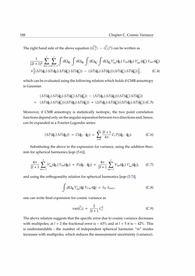
188 Chapter C. Cosmic Variance
The right hand side of the above equation (〈C2l 〉 − 〈Cl〉
2) can be written as
1(2l + 1)2
l∑m=−l
l∑m′=−l
∫dΩq1
∫dΩq2
∫dΩq′1
∫dΩq′2
Y∗lm(q1) Ylm(q2) Y∗lm′(q′
1) Ylm′(q′2)
×
[〈∆T(q1)∆T(q2)∆T(q′1)∆T(q′2)〉 − 〈∆T(q1)∆T(q2)〉〈∆T(q′1)∆T(q′2)〉
], (C.4)
which can be evaluated using the following relation which holds if CMB anisotropyis Gaussian
〈∆T(q1)∆T(q2)∆T(q′1)∆T(q′2)〉 − 〈∆T(q1)∆T(q2)〉〈∆T(q′1)∆T(q′2)〉
= 〈∆T(q1)∆T(q′1)〉〈∆T(q2)∆T(q′2)〉 + 〈∆T(q1)∆T(q′2)〉〈∆T(q2)∆T(q′1)〉.(C.5)
Moreover, if CMB anisotropy is statistically isotropic, the two point correlationfunctions depend only on the angular separation between two directions and, hence,can be expanded in a Fourier-Legendre series:
〈∆T(q1)∆T(q2)〉 = C(q1 · q2) =∞∑
l=0
2l + 14π
Cl Pl(q1 · q2). (C.6)
Substituting the above in the expression for variance, using the addition theo-rem for spherical harmonics [eqn (5.6)],
4π2l + 1
l∑m=−l
Y∗lm(q1) Ylm(q2) = Pl(q1 · q2) =4π
2l + 1
l∑m=−l
Ylm(q1) Y∗lm(q2), (C.7)
and using the orthogonality relation for spherical harmonics [eqn (5.7)],∫dΩq Y∗lm(q) Yl′m′(q) = δll′ δmm′ , (C.8)
one can write final expression for cosmic variance as
var(Cl) =2
2l + 1C2
l . (C.9)
The above relation suggests that the specific error due to cosmic variance decreaseswith multipoles; at l = 2 the fractional error is ∼ 63% and at l = 5 it is ∼ 42%. Thisis understandable - the number of independent spherical harmonic “m” modesincreases with multipoles, which reduces the measurement uncertainty (variance).

189
Appendix D
Elliptical Gaussian fit to theWMAP beam maps
We briefly describe an exercise of characterizing non-circular beams in CMB exper-iments using the example of the beam maps of the WMAP mission. We analyzedthe WMAP raw beam images in the Q1, V1 and W1 [101, 183] bands using twodifferent standard software packages. We use the elliptical Gaussian fit allowedby the well known radio-astronomy software, AIPS and a more elaborate ellipsefitting routine available within the standard astronomical image/data processingsoftware IRAF. The ELLIPSE task in the STSDAS package of IRAF, which uses thewidely known ellipse fitting routines by Jedrzejewski [184], allows independentelliptical fits to the isophotes. This significant greater degree of freedom in fittingto the non-circular beam allows us to assess whether a simple elliptical Gaussianfit is sufficient. The three bands see Jupiter in the two horns (labeled A and B) asa point source. The fitting routine fits ellipses along iso-intensity contours of thebeam image, parameterized by position angle (PA), ellipticity (ε) and position ofthe center. Each of these parameters can be independently varied. The distancebetween successive ellipses can also be independently varied. The eccentricity e isrelated to ellipticity ε as e =
√1 − (1 − ε)2 (Please see Table 8.1).
We fit the the beams in two different ways: (a) by holding the ellipticity constantto ε = 0.05 and freely varying the position angle and center and (b) fixing the centerto be the pixel with the highest intensity (normalized to 1.0 at the central pixel)and varying ellipticity and position angle. In the first case, we get the closestapproximation to circular beam profiles as used in WMAP data analysis. This beamhas no azimuthal (φ) dependence. In the latter case, we get the elliptical profile of

190 Chapter D. Elliptical Gaussian fit to the WMAP beam maps
θsma / rad
Beam Profile
φ
0
0.2
0.4
0.6
0.8
1
0 0.002 0.004 0.006 0.008 0.01 0.012
Inte
nsity
Model g(x)
WMAP Q1 (A) Circular
Recovered
Model h(x)
WMAP Q1 (A) Elliptical =0
Figure D.1: Profile of WMAP Q-beam fitted using IRAF. The beam profile ischaracterized by intensity along the semi major axis (SMA). The beam in Q-bandfor WMAP experiment was analyzed using IRAF and fitted to both circular andelliptical profiles. We have plotted the best fit circular profile (solid error bars) andoverlaid the profile recovered by inverting the WMAP beam transforms, availableat LAMBDA website (solid line). Two analytical models for circular beam profileg(θ) and h(θ) are also considered, and the best fit profiles are overlaid. We find thatthese models are consistent with the IRAF and WMAP data. We have also plottedthe best fit elliptical profile along SMA (broken error bar). Notice that the errorbars in this case are much smaller than those for circular profile, implying a betteragreement with the data.
the WMAP beam which depends on both the polar (θ) and azimuthal (φ) distancefrom the pointing direction. Notice that in this case it is sufficient to provide theintensity along a particular direction (usually, the semi-major axis or φ = 0) and theellipticity ε.
Even a visual inspection reveals that the Q1 beam map plotted in Fig 8.2 isnon-circular and the iso-intensity contours distinctly elliptical. Thus it comes as nosurprise that the error bars as shown in Figure D.1 for circularized beam are largerthan those for the elliptical profile. As a consistency check, we take the WMAP Q1beam transfer function Bl from WMAP first year data archived at publicly availableLAMBDA site [101] and ‘recover’ the circular beam profile B(θ) using eq. (8.10).
From Figure D.1, it is clear that this ‘recovered’ beam profile is in good agree-ment with that obtained by IRAF. This allows us to make some statements aboutthe profile fitting in CMB experiments, in the context of WMAP beams. The beamprofile B(θ) has been modeled as a Gaussian times a sum of even order Hermite
191
0
0.2
0.4
0.6
0.8
1
0 0.002 0.004 0.006 0.008 0.01 0.012θSMA (rad)
Eccentricity
WMAP Q1 (A)WMAP V1 (A)WMAP W1 (A)
-120
-100
-80
-60
-40
-20
0Position Angle (Degree)
WMAP Q1 (B)WMAP V1 (B)WMAP W1 (B)
Figure D.2: IRAF estimated parameters characterizing WMAP beams. The beamsfor WMAP experiment in three bands Q, V and W for both the horns (A and B) werefitted to elliptical profiles using IRAF. The plot above shows the fitted eccentricityand position angle along the semi major axis (SMA). The presence of side-bands inthe smaller beams (W band) makes it difficult for IRAF to model them sufficientlywell. However, in the Q1 band, such sub-structures in the beam are not present thusallowing the IRAF ellipse fitting routine to fit reasonably good ellipses which haveconsistent eccentricities (e ∼ 0.65) and position angles all along the SMA. The V1beam is smaller in extent than the Q1 beam and its eccentricity was determined to bee ∼ 0.46 using IRAF. The highest resolution beam in in W1 band, whose eccentricitywas determined to be e ∼ 0.40.
polynomials (H2n) by the WMAP team [183]. To compare, we have also modeledthe beam profile with a function h(θ) given by
h(θ) = exp(−
12αθ2
)(h0 + h2H2(θ) + h4H4(θ)) , (D.1)
where α, h0, h2 and h4 are unknown parameters to be fixed by least squared method.We found that this model fits the data very well with a reduced χ2 of about 0.7.However, on closer analysis, it is found that the chief role of the Hermite poly-nomials is to add a constant baseline over and above the Gaussian. To test this

192 Chapter D. Elliptical Gaussian fit to the WMAP beam maps
hypotheses, we choose another form of the fitting function g(θ) given by
g(θ) = g0 + g1 exp(−
12
g2θ2), (D.2)
where g0, g1 and g2 are parameters of the model. It is very interesting to note thatthis model also fits the data very well with a reducedχ2 of about 0.8 for the best fittedparameters. In all fairness, g(θ) serves as a simpler model for the beam profile. Wecannot point to the precise origin for the baseline. However, such ‘skirts’ in beamresponses are not uncommon in radio-astronomy. At this point, our observationshould perhaps merit a curious aside, if not as an alternative approach to beammodeling. Our best-fit models g(θ) and h(θ), along with the IRAF fitted data pointsto the WMAP Q1 (A) beam is shown in Figure D.1.
As shown earlier in this thesis, the effects of non-circularity of the CMB ex-perimental beams show up in the power-spectral density estimates through theoff-diagonal elements of the bias matrix All′ . As shown in eq. (8.26), these in turncan be expressed in terms of the leading components of the harmonic transformof the beam. In general, the harmonic decomposition of a non-circular beam mayhave to be done numerically. But for the particular case of an elliptical Gaussianbeam, a closed form expression given by eq. (8.19) serves as a useful test-bed forus. Thus another motivation for fitting ellipses to WMAP beams using IRAF was toget a handle on the eccentricity of these beams so as to find the harmonic transformcomponents of an elliptical Gaussian beam of similar eccentricity. This allows usto give more realistic estimates of the effect of non-circularity of the beam on Cl
estimates.
It is interesting to note how the fitted eccentricities vary as a function of the dis-tance along the semi-major axis of the fitted ellipses for various beams. The smallerbeams (V1 and W1) have sufficient sub-structure in the form of side-lobes whichthrows the ellipse fitting routine off course. However, where the sub-structure isless pronounced, we find that the eccentricities of the fitted ellipses takes a constantvalue. Toward the center of the ellipses, there are far too few pixels to average over,which in turn manifests as large error bars in the eccentricities and position anglesof the ellipses. In Figure D.2, we notice that the Q1 beam has a very elliptical profilewith eccentricity e & 0.65 and position angle of about 75. We also fitted the Q1 (A)beam to an elliptical Gaussian model using radio astronomy standard data analysissoftware AIPS and got consistent numbers for the eccentricity. However the IRAFmodeling gives us more freedom to vary the eccentricity and position angle as we

193
Table D.1: Ellipticities of WMAP beams. The result of ellipse fitting using IRAFon the Q1, V1 and W1 beams of the WMAP experiments. The frequency quotedis the ‘effective’ frequency of the corresponding band from Page et. al. [183]. Thepresence of sub-structures in the W1 band makes it difficult to fit elliptical contoursto the beam.
Beam Frequency Eccentricity Position Angle(GHz) (degree)
Q1 (A) 40.9 0.65 +80Q1 (B) 40.9 0.67 -80V1 (A) 60.3 0.48 +60V1 (B) 60.3 0.45 -60W1 (A) 93.5 0.40 —1
move away from the center of the ellipse and the result is that the beam is modeledmore accurately.

194 Chapter D. Elliptical Gaussian fit to the WMAP beam maps

195
Appendix E
Derivations for perturbativeanalysis of beam correction topseudo-Cl estimator
In the appendix we provide the details of the analytical steps involved inderiving some of the expressions used in chapter 8. This is designed to keep thethesis self contained and easy to extend. These calculations can be useful for otherapplications which involve Wigner-D functions.
Step I
First, we outline the steps involved in evaluating the integralIll′02 + Ill′
0−2 = 2∫ 1−1 dl
00(θ)dl′02(θ)d cosθ to obtain the result in eq. (8.39).
Using the expressions [117,100] for dl00 and dl
02 in terms of Legendre Polynomialsand its derivatives,
∫ 1
−1dl
00(θ)dl′02(θ)d cosθ
= −l′(l′ + 1)
κ
∫ 1
−1Pl(x)Pl′(x)dx +
2κ
∫ 1
−1xPl(x)P′l′(x)dx, (E.1)
where, κ ≡√
(l − 1)l(l + 1)(l + 2). The first integral is simply the orthogonality of

196Chapter E. Derivations for perturbative analysis of beam correction to pseudo-Cl
estimator
Legendre polynomials ∫ 1
−1Pl(x)Pl′(x)dx =
2δll′
2l + 1. (E.2)
Further, we can show that for odd values of l + l′,∫ 1
−1x Pl(x) P′l′(x) dx = 0, (E.3)
and for even values of l + l′,
∫ 1
−1x Pl(x) P′l′(x) dx =
2 if l < l′
0 if l > l′
2l/(2l + 1) if l = l′.(E.4)
Assembling all these we can derive eq. (8.39).
Step II
Next we evaluate the more general integral Ill′m2+Ill′
m−2 ≡∫ 1−1 dl
m0(θ) [dl′m2(θ)+dl′
m−2(θ)] d cosθto obtain the expression in eq. (8.40). The first step is to express dl
m±2(θ) in termsof dl′
m0(θ). Using the recurrence relations for Wigner D functions (see eq. (4)in§4.8.1, [100]) and using the fact that
Dlmm′(φ, θ, ρ) = e−imφ dl
mm′(θ) e−im′ρ (E.5)
we get the recurrence relations for Wigner-d functions:
sinθ dlmm′+1(θ) =
√(l2 −m2)(l +m′)(l +m′ + 1)
l(2l + 1)dl−1
mm′(θ) (E.6)
−m
√(l −m′)(l +m′ + 1)
l(l + 1)dl
mm′(θ)
−
√[(l + 1)2 −m2](l −m′)(l −m′ + 1)
(l + 1)(2l + 1)dl+1
mm′(θ).
Using these relations for dlm2 we may write,
dlm2(θ) =
κ
sin2(θ)[κ0dl
m0(θ)+ κ1dl+1m0 (θ)+ κ−1dl−1
m0 (θ)+ κ2dl+2m0 (θ) + κ−2dl−2
m0 (θ)], (E.7)

197
where
κ0 ≡m2
l2(l + 1)2 −l2 −m2
l2(4l2 − 1)−
(l + 1)2−m2
(l + 1)2(2l + 1)(2l + 3),
κ1 ≡ 2m
√(l + 1)2 −m2
l(l + 1)(l + 2)(2l + 1), κ−1 ≡ −2m
√
l2 −m2
l(l2 − 1)(2l + 1),
κ2 ≡
√[(l + 1)2 −m2][(l + 2)2 −m2](l + 1)(l + 2)(2l + 1)(2l + 3)
, κ−2 ≡
√(l2 −m2)[(l − 1)2 −m2]
l(l − 1)(4l2 − 1).
Also, since dlm−2(θ) = (−1)l+mdl
m2(π−θ) and dlm0(π−θ) = (−1)l+mdl
m0(θ) we can write,
dlm−2(θ) =
κ
sin2(θ)[κ0dl
m0(θ)−κ1dl+1m0 (θ)−κ−1dl−1
m0 (θ)+κ2dl+2m0 (θ) + κ−2dl−2
m0 (θ)]. (E.8)
Using the expression for dm±2 we can make the following substitution
dlm2(θ) + dl
m−2(θ) = 2κ [κ0dlm0(θ) + κ2dl+2
m0 (θ) + κ−2dl−2m0 (θ)]/ sin2 θ , (E.9)
in the integral we seek to evaluate. We use the following integral for l ≤ l′ andL = minl, l′ ≥ |m| > 0,
∫ 1
−1dl
m0(θ)dl′m0(θ)
d cosθsin2 θ
=
1|m|
√(l+|m|)!(l′−|m|)!(l−|m|)!(l′+|m|)! even l + l′
0 odd l + l′(E.10)
and obviously, for l > l′, l and l′ have to be interchanged in the above expression.We then obtain Ill′
m2 + Ill′m−2 as given in eq. (8.40).
Step III
The integral in eq. (E.10) can also be readily derived. We use the fact that
dlm0(θ) = (−1)m
√(l −m)!(l +m)!
Pml (cosθ) , (E.11)
which leads to∫ 1
−1dl
m0(θ)dl′m0(θ)
d cosθsin2 θ
=
√(l −m)!(l′ −m)!(l +m)!(l′ +m)!
∫ 1
−1Pm
l (x)Pml′ (x)
dx1 − x2 . (E.12)

198Chapter E. Derivations for perturbative analysis of beam correction to pseudo-Cl
estimator
The symmetry of Associated Legendre Polynomials, Pml (−x) = (−1)l+mPm
l (x) dictatesthat the integrand is antisymmetric for odd values of l+ l′, hence the integral is zero.However for even values of l + l′, we can evaluate the integral in the followingmanner. One of the recurrence relations for Associated Legendre Polynomials is( [185], §12.5.)
Pml (x) = Pm
l−2(x) + (2l − 1)√
1 − x2Pm−1l−1 (x) . (E.13)
Using equation (E.13) we can write,∫ 1
−1Pm
l (x)Pml′ (x)
dx1 − x2 (E.14)
=
∫ 1
−1Pm
l (x)Pml′−2(x)
dx1 − x2 + (2l′ − 1)
∫ 1
−1Pm
l (x)Pm−1l′−1 (x)
dx√
1 − x2.
We have provided a proof that the second integral on the right is zero at the end ofthis section. Thus, from eq. (E.14) we have∫ 1
−1Pm
l (x)Pml′ (x)
dx1 − x2 =
∫ 1
−1Pm
l (x)Pml′−2(x)
dx1 − x2 . (E.15)
In this way we can keep reducing l′ by two each time until it equals with l (sincel + l′ is even and l < l′ it will reduce to l). Thus, we have shown that,∫ 1
−1Pm
l (x)Pml′ (x)
dx1 − x2 =
∫ 1
−1
[Pm
l (x)]2 dx
1 − x2 =1m
(l +m)!(l −m)!
, (E.16)
where the second equality follows from the evaluation of a standard integral, whichcan be obtained, for example, from [185]. Substituting in eq. (E.12) we can evaluatethe integral for m > 0. Clearly eq. (E.16) is valid for l = l′. For l > l′, l should bereplaced by l′ in that equation. Moreover, using the property dl
−m0(θ) = (−1)mdlm0(θ),
we can express the integral for any m , 0, as given in eq. (E.10).
Step IV
Finally we prove the result used in simplifying eq. (E.14) that for even values ofl + l′ and l < l′, ∫ 1
−1Pm
l (x)Pm−1l′−1 (x)
dx√
1 − x2= 0. (E.17)
Using the recurrence relation of Legendre Polynomials in eq. (E.13), we can

199
write ∫ 1
−1Pm
l (x)Pm−1l′−1 (x)
dx√
1 − x2(E.18)
=
∫ 1
−1Pm
l−2(x)Pm−1l′−1 (x)
dx√
1 − x2+ (2l − 1)
∫ 1
−1Pm−1
l−1 (x)Pm−1l′−1 (x)dx.
Then from the orthogonality relation of associated Legendre Polynomials,∫ 1
−1Pm
l (x)Pml′ (x)dx =
22l + 1
(l +m)!(l −m)!
δll′ , (E.19)
we can see that the second integral on the right of eq. (E.18) vanishes for l′ , l. Thuswe have, ∫ 1
−1Pm
l (x)Pm−1l′−1 (x)
dx√
1 − x2=
∫ 1
−1Pm
l−2(x)Pm−1l′−1 (x)
dx√
1 − x2. (E.20)
We can use the above equation iteratively since the lower indices of the Pml ’s will
never match as l′ > l. So the lower index of the first polynomial in the integrationcan be reduced to either m or m+ 1 (depending on l−m is even or odd) by repeateduse of the above identity. Thus we may write
∫ 1
−1Pm
l (x)Pm−1l′−1 (x)
dx√
1 − x2=
∫ 1−1 Pm
m(x)Pm−1l′−1 (x) dx
√
1−x2
or∫ 1−1 Pm
m+1(x)Pm−1l′−1 (x) dx
√
1−x2.
(E.21)
Finally using the relations,
Pmm = (−1)m (2m − 1)!! (1 − x2)m/2
= (−1)(2m − 1)√
1 − x2Pm−1m−1, (E.22)
Pmm+1 = x(2m + 1)Pm
m = x(2m + 1)(−1)(2m − 1)√
1 − x2Pm−1m−1
= (−1)(2m + 1)√
1 − x2Pm−1m (E.23)
and the orthonormality condition in eq. (E.2) we can see that in both the cases rightside of eq. (E.21) is zero. This completes the proof.

200Chapter E. Derivations for perturbative analysis of beam correction to pseudo-Cl
estimator
201
Appendix F
Derivations for general analysis ofbeam correction to pseudo-Clestimator
F.1 Useful formulae
• Important relations [eq. (1)s of §4.3, §4.17 & §5.4 and eq. (2) of §4.4 of [100]]:
Dlmm′(q, ρ) = e−imφ dl
mm′(θ) e−im′ρ (F.1)
Y∗lm(q) =
√2l + 1
4πDl
m0(q, ρ) =
√2l + 1
4πe−imφ dl
m0(θ) (F.2)
Dl∗mm′(q, ρ) = (−1)m−m′ Dl
−m−m′(q, ρ) (F.3)
Y∗lm(q) = (−1)m Yl−m(q) (F.4)
Note that, unlike [118], the argument of the Wigner-d function is θ (standarddefinition) not cosθ.
• The Clebsch-Gordon series:
Expansion of the product of two Wigner-D functions [eqn (1) of §4.6 of [100]]:
Dl1m1n1
(q, ρ) Dl2m2n2
(q, ρ) =l1+l2∑
l=|l1−l2|
Cl(m1+m2)l1m1l2m2
Dl(m1+m2)(n1+n2)(q, ρ) Cl(n1+n2)
l1n1l2n2, (F.5)

202Chapter F. Derivations for general analysis of beam correction to pseudo-Cl estimator
where Clml1m1l2m2
are the Clebsch-Gordon coefficients.The special case of spherical harmonics [eq. (9) of §5.6 of [100]]:
Yl1m1(q) Yl2m2(q) = (F.6)l1+l2∑
l=|l1−l2|
√(2l1 + 1)(2l2 + 1)
4π(2l + 1)Cl0
l10l20 Cl(m1+m2)l1m1l2m2
Yl(m1+m2)(q).
In modifying the above equations (from [100]) we have used the fact that theClebsch-Gordon coefficients Clm
l1m1l2m2vanish if m , m1 +m2.
• The integral∫ π
0 dθ sinθ eiNθ equals to:∫ π
0dθ
[ei(N+1)θ
− ei(N−1)θ
2i
]= (F.7)
±iπ/2 if N = ±1[1−ei(N+1)π
2(N+1) −1−ei(N−1)π
2(N−1)
]=
0 if N = odd (, ±1)2
1−N2 if N = 0, even.
The above can be used to define an useful quantity
f (m′; N) := <
[im′
(−1)N∫ π
0sinθdθ eiNθ
](F.8)
=
(−1)(m′±1)/2 π/2 if m′ = odd and N = ±1
(−1)m′/2 2/(1 −N2) if both m′,N = 0 or even0 otherwise.
F.2 Expansion of Wigner-D Function
Motivation
This derivation is motivated from eq. (10) of §4.16 of [100]. However, the motivatingequation is wrong, as it predicts Dl
mm′(φ, θ, ρ) = 0 if m + m′ = odd. We derive thecorrect formula by “reverse engineering”. We start with the second expression of

F.2: Expansion of Wigner-D Function 203
the above mentioned equation [see below for steps]:
l∑M1,M2,M3,M4=−l
[Dl
mM1
(φ, 0, 0
)Dl
M1M2
(0,π2, 0
)Dl
M2M3(0, θ, 0)
DlM3M4
(0,π2, 0
)Dl
M4m′(0, 0, ρ
)]= e−imφ
l∑M2,M3=−l
[Dl
mM2
(0,π2, 0
)Dl
M2M3(θ, 0, 0) Dl
M3m′
(0,π2, 0
)]e−im′ρ
= e−imφl∑
M2=−l
[Dl
mM2
(0,π2, 0
)Dl
M2m′
(θ,π2, 0
)]e−im′ρ
= e−imφ Dlmm′
(π2, π − θ,
π2
)e−im′ρ = Dl
mm′
(π2+ φ, π − θ,
π2+ ρ
)(F.9)
Steps
Step IFrom eq. (1) & (2) of §4.16, pg.112 of [100].
Dlmm′(φ, 0, 0) = e−imφ Dl
mm′(0, 0, 0) (F.10)
Dlmm′(0, 0, ρ) = Dl
mm′(0, 0, 0) e−im′ρ (F.11)
Dlmm′(0, 0, 0) = δmm′ . (F.12)
Step II1
e−imφl∑
M3=−l
[Dl
mM3
(0,π2, θ
)Dl
M3m′
(0,π2, 0
)]e−im′ρ (F.13)
From the “Addition of Rotations" formula in eq. (3) of §4.7, pg.87 of [100].
l∑M=−l
[Dl
mM(φ, θ1, γ) DlMm′(−γ, θ2, ρ)
]= Dl
mm′(φ, θ1 + θ2, ρ). (F.14)
1Another way is to combine the first two remaining D symbols using eq. (1) of §4.16, pg.112 of [100]and then evaluate the following in Step III using the “Addition of Rotations" formula similar to thepresent method:

204Chapter F. Derivations for general analysis of beam correction to pseudo-Cl estimator
Step IIIFrom eq. (1) of §4.7, pg.87 of [100] we may write
l∑M=−l
[Dl
mM(0,π2, 0) Dl
Mm′(θ,π2, 0)
]= Dl
mm′(α, β, γ) (F.15)
where α, β, γ are to be obtained using eq. (66)-(70) of §1.4, pg.32 of [100]. Note thatthe arguments of the first D symbol have been denoted by α2, β2, γ2 respectively andnot by α1, β1, γ1.From eq. (66) of §1.4, pg.32 of [100], since 0 ≤ α < 2π, 0 ≤ β ≤ π, 0 ≤ γ < 2π
cosα = 0 ⇒ α =π2
or3π2
(F.16)
cos β = − cosθ ⇒ β = π − θ (F.17)
cosγ = 0 ⇒ γ =π2
or3π2. (F.18)
From eq. (67) of §1.4, pg.32 of [100]
sinα = sinγ =sinθsinθ
= 1. (F.19)
Combining the above equations we may write
α =π2
; β = π − θ; γ =π2. (F.20)
Final expression
We can modify eq. (F.9) by changing φ→ φ − π2 , θ→ π − θ, ρ→ ρ − π
2 to reach thedesired expansion:
Dlmm′
(φ, θ, ρ
)= e−im(φ−π/2)e−im′(ρ−π/2)
× (F.21)l∑
M2,M3=−l
[Dl
mM2
(0,π2, 0
)Dl
M2M3(π − θ, 0, 0) Dl
M3m′
(0,π2, 0
)].
Then using the definitions of Wigner-d functions from eq. (1) of §4.3, pg.76 andeq. (1) of §4.16, pg.112 of [100], we get
Dlmm′
(φ, θ, ρ
)= im+m′ e−imφ
l∑M=−l
[(−1)M dl
mM
(π2
)eiMθ dl
Mm′
(π2
)]e−im′ρ. (F.22)

F.3: Evaluation of Jll′′l′nm′′mm′ using sinusoidal expansion of Wigner-d 205
This also means
dlmm′(θ) = im+m′
l∑M=−l
[(−1)M dl
mM
(π2
)eiMθ dl
Mm′
(π2
)]. (F.23)
The coefficients dlmm′(π/2) can be directly calculated using eq. (5) of §4.16, pg.113
of [100]
dlmm′
(π2
)= (−1)m−m′ 1
2l
√(l +m)!(l −m)!
(l +m′)!(l −m′)!× (F.24)
maxl+m′, l−m∑k=max0,m′−m
(−1)k
l +m′
k
l −m′
k +m −m′
.F.3 Evaluation of Jll′′l′
nm′′mm′ using sinusoidal expansion of Wigner-d
Putting eq. (9.21) in eq. (9.20) we get
Jll′′l′nm′′mm′ :=
∫S2
dΩq Yln(q) Yl′′m′′(q) Dl′mm′(q, ρ(q)) (F.25)
=
√(2l + 1)(2l′′ + 1)
4π
∫ 2π
0dφ ei(n+m′′−m)φ
×∫ π
0sinθdθ dl
n0(θ) dl′′m′′0(θ) dl′
mm′(θ) e−im′ρ(q)
=
√(2l + 1)(2l′′ + 1)
4πin+m+m′+m′′
l∑M=−l
dlnM
(π2
)dl
M0
(π2
)×
l′′∑M′′=−l′′
dl′′m′′M′′
(π2
)dl′′
M′′0
(π2
) l′∑M′=−l′
dl′mM′
(π2
)dl′
M′m′
(π2
)×
(−1)M+M′′+M′∫ 2π
0dφ ei(n+m′′−m)φ
∫ π
0sinθdθ ei(M+M′+M′′)θ e−im′ρ(q).
To proceed further analytically, we need a model for ρ(q). We shall continueassuming non-rotating beams, i.e. ρ(q) = 0. In this case the φ integral above isseparable. Using, ∫ 2π
0dφ ei(n+m′′−m)φ = 2πδm′′(m−n) (F.26)

206Chapter F. Derivations for general analysis of beam correction to pseudo-Cl estimator
we can get a simplified result:
Jll′′l′nm′′mm′ = 2πδm′′(m−n)
√(2l + 1)(2l′′ + 1)
4π
l∑M=−l
dlnM
(π2
)dl
M0
(π2
)×
l′′∑M′′=−l′′
dl′′m′′M′′
(π2
)dl′′
M′′0
(π2
) l′∑M′=−l′
dl′mM′
(π2
)dl′
M′m′
(π2
)×[
in+m+m′+m′′ (−1)M+M′′+M′∫ π
0sinθdθ ei(M+M′+M′′)θ
]. (F.27)
The above expression is real. The proof follows:
• Contribution for all of M,M′,M′′ = 0:In this term (of the summation) the integral of the above expression is real.Therefore, if n +m +m′ +m′′ = even this term is real (because then the factorin+m+m′+m′′ is real). When n +m +m′ +m′′ = odd, which means at least one ofn,m+m′,m′′ is odd, this term does not contribute, since dl
m0(π/2)dl0m′(π/2) = 0
if m +m′ = odd (follows from eq. (6) of §4.16 of [100]).
• Contribution for not all of M,M′,M′′ = 0:For each set of M,M′,M′′ in the above summation, there exists a set−M,−M′,−M′′,which converts the integral of the above expression to its complex conju-gate. Since dl
mm′(π/2) = (−1)l−m′dl−mm′(π/2) = (−1)l+mdl
m−m′(π/2) [see eq. (1)of §4.4 of [100]], the Wigner-d symbols give a factor of (−1)n+m+m′+m′′ . So, ifn + m + m′ + m′′ = even, the sum is real, as well as the factor in+m+m′+m′′ andboth are imaginary if n +m +m′ +m′′ = odd.
Therefore, the full summation is always real.
Following the discussion on the reality of the expression and using eq. (F.8) wecan write
Jll′′l′nm′′mm′ = 2πδ(m−n)m′′ (−1)m
√(2l + 1)(2l′′ + 1)
4π×
l∑M=−l
dlnM
(π2
)dl
M0
(π2
) l′′∑M′′=−l′′
dl′′(m−n)M′′
(π2
)dl′′
M′′0
(π2
)×
l′∑M′=−l′
dl′mM′
(π2
)dl′
M′m′
(π2
)f (m′; M +M′ +M′′). (F.28)

F.4: Evaluation of Jll′′l′nm′′mm′ using Clebsch-Gordon series and sinusoidal expansion of
Wigner-d 207
Moreover, since for “symmetric" beams βlm = 0 for m = odd, in the final expressionterms with m′ = odd shall not contribute, that means, for symmetric beams, f (m′; N)contributes only when both m′,N = 0 or even.
To make the final expression more simple, we can write the bias matrix fornon-rotating beam with incomplete sky coverage as:
All′ = B2l
(2l′ + 1)16π
l∑n=−l
l′∑m=−l′
∣∣∣∣∣∣∣∞∑
l′′=0
√
2l′′ + 1 Ul′′(m−n) × (F.29)
l′′∑M′′=−l′′
dl′′(m−n)M′′
(π2
)dl′′
M′′0
(π2
) l∑M=−l
dlnM
(π2
)dl
M0
(π2
)×
l′∑M′=−l′
dl′mM′
(π2
) l′∑m′=−l′
βl′m′ dl′M′m′
(π2
)f (m′; M +M′ +M′′)
∣∣∣∣∣∣∣2
.
This form could be useful for numerical evaluation.
F.4 Evaluation of Jll′′l′nm′′mm′ using Clebsch-Gordon series and
sinusoidal expansion of Wigner-d
Putting eqn (F.6), (F.4), (F.2), (F.5) & (9.21) in eqn (9.19) we get
Jll′′l′nm′′mm′ ≡
∫S2
dΩq Yln(q) Yl′′m′′(q) Dl′mm′(q, ρ(q)) (F.30)
=
l+l′′∑L=|l−l′′|
√(2l + 1)(2l′′ + 1)
4π(2L + 1)CL0
l0l′′0 CL(n+m′′)lnl′′m′′ ×∫
S2dΩq YL(n+m′′)(q)Dl′
mm′(q, ρ(q))
= (−1)n+m′′√
(2l + 1)(2l′′ + 1)4π
×
l+l′′∑L=|l−l′′|
CL0l0l′′0CL(n+m′′)
lnl′′m′′
∫S2
dΩqDL(−n−m′′)0(q, ρ(q))Dl′
mm′(q, ρ(q))
= (−1)n+m′′√
(2l + 1)(2l′′ + 1)4π
l+l′′∑L=|l−l′′|
CL0l0l′′0 CL(n+m′′)
lnl′′m′′ ×
L+l′∑L′=|L−l′|
CL′(m−n−m′′)L(−n−m′′)l′m CL′m′
L0l′m′
∫S2
dΩq DL′(m−n−m′′)m′(q, ρ(q)).

208Chapter F. Derivations for general analysis of beam correction to pseudo-Cl estimator
Now using eq. (9.21) one can write integrals of the above form as (m−n−m′′ →M′
& m′ →M′′):∫S2
dΩq DL′M′M′′(q, ρ(q)) = (F.31)
iM′+M′′
L′∑N=−L′
(−1)N dL′M′N
(π2
)dL′
NM′′
(π2
) ∫S2
dΩq e−iM′φ eiNθ e−iM′′ρ(q).
To proceed further analytically, we need a model for ρ(q). We shall continueassuming non-rotating beams, i.e. ρ(q) = 0. In this case the φ integral above isseparable. Then, putting eq. (F.26) we get∫
S2dΩq DL′
M′M′′(q, 0) = (F.32)
2πδM′0 iM′′
L′∑N=−L′
(−1)N dL′0N
(π2
)dL′
NM′′
(π2
) ∫ π
0sinθdθ eiNθ.
This integral is real. This becomes clear if we write the right hand side of the aboveequation as
2πδM′0iM′′
2 dL′00
(π2
)dL′
0M′′
(π2
)+
L′∑N=1
(−1)NdL′0N
(π2
)dL′
NM′′
(π2
)∫ π
0sinθdθ
eiNθ + (−1)M′′e−iNθ
]. (F.33)
When M′′ = even both iM′′
and the integrand are real, and when M′′ = oddboth iM
′′
and the integrand are imaginary. The first term inside the square bracketdoes not contribute when M′′ = odd (since dL′
00(π/2)dL′0M′′(π/2) vanishes in that case).
Therefore irrespective of the value of M′′ the above expression is real. Thus,∫S2
dΩq DL′M′M′′(q, 0) = (F.34)
2πδM′0
L′∑N=−L′
dL′0N
(π2
)dL′
NM′′
(π2
)<
[iM′′
(−1)N∫ π
0sinθdθ eiNθ
].

F.5: The full sky and circular beam limit 209
Now we can use the above results and combine with eq. (F.8) to get
Jll′′l′nm′′mm′ = (−1)n+m′′ δm′′(m−n)
√(2l + 1)(2l′′ + 1)
2×
l+l′′∑L=|l−l′′|
CL0l0l′′0 CL(n+m′′)
lnl′′m′′
L+l′∑L′=|L−l′|
CL′(m−n−m′′)L(−n−m′′)l′m CL′m′
L0l′m′ ×
L′∑N=−L′
dL′0N
(π2
)dL′
Nm′
(π2
)f (m′; N). (F.35)
The final form of the bias matrix for non-rotating beam with incomplete skycoverage can now be written as (after replacing m′′ by m−n, pulling out few factorsoutside the modulus and squaring):
All′ = B2l
(2l′ + 1)16π
l∑n=−l
l′∑m=−l′
∣∣∣∣∣∣∣∞∑
l′′=0
√
2l′′ + 1 Ul′′(m−n) ×
l+l′′∑L=|l−l′′|
CL0l0l′′0 CLm
lnl′′(m−n)
L+l′∑L′=|L−l′|
CL′0L−ml′m
L′∑N=−L′
dL′0N
(π2
)×
l′∑m′=−l′
βl′m′ CL′m′L0l′m′ dL′
Nm′
(π2
)f (m′; N)
∣∣∣∣∣∣∣2
. (F.36)
F.5 The full sky and circular beam limit
Here we recover the special case of circular beam and complete sky coverage limit.From Eq. F.36, the full sky limit [Ulm =
√4πδl0] is obtained by replacing Ul′′(m−n)
with√
4πδl′′0δmn; and for the circular beam, we replace the BDP βl′m′ with δm′0. So,
All′ = B2l
2l′ + 1)4
min(l,l′)∑n=−min(l,l′)
∣∣∣∣∣∣∣Cl0l000 Cln
ln00
l+l′∑L′=|l−l′|
CL′0l−nl′n CL′0
l0l′0 ×
L′∑N=−L′
dL′0N
(π2
)dL′
N0
(π2
)f (0; N)
∣∣∣∣∣∣∣2
. (F.37)

210Chapter F. Derivations for general analysis of beam correction to pseudo-Cl estimator
From the relation Ccγaα00 = δacδαγ (Eq. (2) in §8.5.1 of [100]), we can reduce Cl0
l000 andCln
ln00 to unity, and get:
All′ = B2l
2l′ + 14
min(l,l′)∑n=−min(l,l′)∣∣∣∣∣∣∣
l+l′∑L′=|l−l′|
CL′0l−nl′n CL′0
l0l′0
L′∑N=−L′
dL′0N
(π2
)dL′
N0
(π2
)f (0; N)
∣∣∣∣∣∣∣2
. (F.38)
To get the value of∑L′
N=−L′ dL′0N
(π2
)dL′
N0
(π2
)f (0; N), we have to start a step back.
Y∗lm(q) =
√2l + 1
4πDl
mm′(q, 0)
=
√2l + 1
4πime−imφ
l∑N=−l
(−1)NdlmN
(π2
)dl
N0
(π2
)eiNθ (F.39)
From the relation ∫S2
Y∗lm(q)dΩq =√
4πδl0δm0
it follows that√2l + 1
4πim
l∑N=−l
(−1)NdlmN
(π2
)dl
N0
(π2
) ∫eiNθsinθdθ
∫e−imφdφ
=√
4πδl0δm0. (F.40)
The last integral (i.e.,∫
e−imφdφ) gives 2πδm0. So, equating out both sides andrearranging, we have
iml∑
N=−l
(−1)NdlmN
(π2
)dl
N0
(π2
) ∫eiNθsinθdθ
∫e−imφdφ =
2√
2l + 1δl0. (F.41)

F.6: The circular beam limit with cut sky 211
The l.h.s. is identified with the relation∑L′
N=−L′ dL′0N
(π2
)dL′
N0
(π2
)f (0; N), and hence
Eq.(F.38) reduces to
All′ = B2l
2l′ + 14
min(l,l′)∑n=max(−l,−l′)
∣∣∣∣∣∣∣l+l′∑
L′=|l−l′|
CL′0l−nl′n CL′0
l0l′02
√2L′ + 1
δL′0
∣∣∣∣∣∣∣2
= B2l (2l′ + 1)
min(l,l′)∑n=max(−l,−l′)
∣∣∣C00l−nl′n C00
l0l′0
∣∣∣2 . (F.42)
We know from Eq. (1) of §8.5.1 of [100]
C00aαbβ = (−1)a−α δabδα,−β
√2a + 1
.
Hence, All′ finally reduces to the desired result
All′ = B2l δll′ .
F.6 The circular beam limit with cut sky
We will show in this section that our formulation reduces to the analytic limit ofthe MASTER method of Hivon et al. [167] for the incomplete sky coverage takingcircular beams. Following the procedure mentioned in section F.5, we proceed as:
All′ = B2l
2l′ + 116π
l∑n=−l
l′∑m=−l′
∣∣∣∣∣∣∣∞∑
l′′=0
√
2l′′ + 1 Ul′′(m−n)
l+l′′∑L=|l−l′′|
CL0l0l′′0 CLm
lnl′′(m−n)
×
L+l′∑L′=|L−l′|
CL′0L−ml′m CL′0
L0l′0
L′∑N=−L′
dL′0N
(π2
)dL′
N0
(π2
)f (0; N)
∣∣∣∣∣∣∣2
(F.43)

212Chapter F. Derivations for general analysis of beam correction to pseudo-Cl estimator
Using Eq. (F.41), we get
All′ = B2l
2l′ + 14π
l∑n=−l
l′∑m=−l′∣∣∣∣∣∣∣
∞∑l′′=0
√
2l′′ + 1 Ul′′(m−n)
l+l′′∑L=|l−l′′|
CL0l0l′′0 CLm
lnl′′(m−n)C00L(−m)l′m C00
L0l′0
∣∣∣∣∣∣∣2
=B2
l
4π
l∑n=−l
l′∑m=−l′
∣∣∣∣∣∣∣∞∑
l′′=0
√
2l′′ + 1 Ul′′(m−n)
l+l′′∑L=|l−l′′|
CL0l0l′′0 CLm
lnl′′(m−n)
∣∣∣∣∣∣∣2
To arrive at Eq. A31 of Hivon et al. [167], we first replace (m-n) by m′′ and then openup the modulus square. The symbol Cl′m
lnl′′m′′ contributes only when m′′ is equal to(m-n) and also l′′ satisfies the triangle inequality.
All′ =B2
l
4π (2l′ + 1)
l∑n=−l
l′∑m=−l′
∣∣∣∣∣∣∣∞∑
l′′=0
√
2l′′ + 1l′′∑
m′′=−l′′Ul′′m′′Cl′0
l0l′′0 Cl′mlnl′′m′′
∣∣∣∣∣∣∣2
=B2
l
4π(2l′ + 1)
l∑n=−l
l′∑m=−l′
∞∑
l′′1 =0
√2l′′1 + 1 Cl′0
l0l′′1 0
∞∑l′′2 =0
√2l′′2 + 1 Cl′0
l0l′′2 0
l′′2∑m′′2 =−l′′2
l′′1∑m′′1 =−l′′1
Ul′′1 m′′1U∗l′′2 m′′2
Cl′mlnl′′1 m′′1
Cl′mlnl′′2 m′′2
=
B2l
4π(2l′ + 1)
∞∑l′′1 =0
∞∑l′′2 =0
√2l′′1 + 1
√2l′′2 + 1 Cl′0
l0l′′1 0 Cl′0l0l′′2 0
l′′2∑m′′2 =−l′′2
l′′1∑m′′1 =−l′′1
Ul′′1 m′′1U∗l′′2 m′′2
l∑n=−l
l′∑m=−l′
Cl′mlnl′′1 m′′1
Cl′mlnl′′2 m′′2
(F.44)
The last summation∑l
n=−l∑l′
m=−l′ Cl′mlnl′′1 m′′1
Cl′mlnl′′2 m′′2
simplifies to (2l′+1)/(2l′′1 +1)δl′′1 l′′2δm′′1 m′′2
by Eq. (5) of § 8.7.2 of [100]. So, we have
All′ =B2
l
4π
l+l′∑l′′=|l−l′|
(Cl′0
l0l′′0
)2l′′∑
m′′=−l′′|Ul′′m′′ |
2
= B2l
2l′ + 14π
l+l′∑l′′=|l−l′|
(2l′′ + 1)
l l′ l′′
0 0 0
2
Ul′′ , (F.45)

F.7: The full sky limit with non-circular beam 213
whereUl′′ :=∑l′′
m′′=−l′′ |Ul′′m′′ |2/(2l′′ + 1). This matches the final expression of [167]
[See eqn (A31)].
F.7 The full sky limit with non-circular beam
The full sky limit to the final expression should reproduce the result obtainedin [118]. We substitute Ulm =
√4πδl0 [⇒ Ul′′(m−n) =
√4πδl′′0δmn] in eqn (9.25) and
get
All′ = B2l
(2l′ + 1)4
min(l,l′)∑m=−min(l,l′)
∣∣∣∣∣∣∣Cl0l000 Clm
lm00
l+l′∑L=|l−l′|
CL0l−ml′m ×
L∑N=−L
dL0N
(π2
) l′∑m′=−l′
βl′m′ CLm′l0l′m′ dL
Nm′
(π2
)f (m′; N)
∣∣∣∣∣∣∣2
. (F.46)
Using the relation Ccγaα00 = δacδαγ [Eq. (2) in §8.5.1 of [100])] we may write Cl0
l000 =
Clmlm00 = 1. Then rearranging terms, we may write
All′ = B2l
(2l′ + 1)4
min(l,l′)∑m=−min(l,l′)
∣∣∣∣∣∣∣l′∑
m′=−l′βl′m′
l+l′∑L=|l−l′|
CL0l−ml′m CLm′
l0l′m′ ×
L∑N=−L
dL0N
(π2
)dL
Nm′
(π2
)f (m′; N)
∣∣∣∣∣∣∣2
. (F.47)
Using the definition of f (m′; N) [eqn (9.24)] and the expansion formula for Wigner-d[eqn (9.21)] we may write
L∑N=−L
dL0N
(π2
)dL
Nm′
(π2
)f (m′; N) =
∫ 1
−1d cosθ dL
0m′(θ). (F.48)
Then, using the Clebcsh-Gordon series [eqn (F.5)] we get
l+l′∑L=|l−l′|
CL0l−ml′m dL
0m′(θ) CLm′l0l′m′ = (−1)m dl
m0(θ) dl′mm′(θ). (F.49)

214Chapter F. Derivations for general analysis of beam correction to pseudo-Cl estimator
Finally, putting everything together, we get the expression for the bias matrix in thefull sky limit with non-circular beam as
All′ = B2l
(2l′ + 1)4
min(l,l′)∑m=−min(l,l′)
∣∣∣∣∣∣∣l′∑
m′=−l′βl′m′
∫ 1
−1d cosθ dl
m0(θ) dl′mm′(θ)
∣∣∣∣∣∣∣2
, (F.50)
which matches eqn (38) of [118].

215
Appendix G
Fast computation of non-circularbeam correction toCMB power spectrum
The general analytical results obtained in chapter 9 to estimate the bias in CMBpower spectrum due to noncircular beams including the effect of incomplete skycoverage will be important only if the evaluation time is much faster than carryingfull blown simulations. The fast evaluation of the analytical results is, however, notstraight forward. Smart innovations are necessary for the numerical implementa-tion of the analysis. The basic principle of the fast implementation algorithm havebeen outlined in section 9.2, the detailed calculations are presented in this appendix.
The full expression for the bias matrix with no rotation:
All′ = B2l
2l′ + 116π
l∑n=−l
l′∑m=−l′
∣∣∣∣∣∣∣∞∑
l′′=0
√
2l′′ + 1 Ul′′(m−n) × (G.1)
l′′∑M′′=−l′′
dl′′(m−n)M′′
(π2
)dl′′
M′′0
(π2
) l∑M=−l
dlnM
(π2
)dl
M0
(π2
)×
l′∑M′=−l′
dl′mM′
(π2
) l′∑m′=−l′
βl′m′ dl′M′m′
(π2
)f (m′; M +M′ +M′′)
∣∣∣∣∣∣∣2
.
The following way of calculation requires less computation cost. V1,2,3 have beenused as intermediate arrays. This prescription is only for the loops inside themodulus, so for each m,n pair all the three steps have to be performed.

216Chapter G. Fast computation of non-circular beam correction to
CMB power spectrum
• Step I:
V1(N) =l′∑
M′=−l′dl′
mM′
(π2
) l′∑m′=−l′
βl′m′ dl′M′m′
(π2
)f (m′; M′ +N), (G.2)
N runs from −(l + l′′max) to +(l + l′′max).
• Step II
V2(M′′) =l∑
M=−l
dlnM
(π2
)dl
M0
(π2
)V1
ll′[M +M′′; m]. (G.3)
• Step III
V3 =
l′′max∑l′′=0
√
2l′′ + 1 Ul′′(m−n)
l′′∑M′′=−l′′
dl′′(m−n)M′′
(π2
)dl′′
M′′0
(π2
)V2
ll′[M′′; n]. (G.4)
Required number of cycles to compute V3 for each pair m,n for lmax l′′max and thecut off for the m′ summation at m′max = mbeam is:2(l + l′′max) + 1(2l′ + 1)(2mbeam + 1) + (2l′′max + 1)(2l + 1) +
l′′max∑l′′=0
(2l′′ + 1)
(G.5)
As mentioned earlier we are interested in the total number of computation cyclesin the limit lmax l′′max. Before procceeding further we note that Ul′′m′′ = Ul′′m−n islimited to only mmask modes for each l′′. Here mmask > 0. Thus means that N variesfrom −(l+mmask) to (l+mmask) in Step I. Moreover, the condition for non-negligiblevalues of Ul′′m−n becomes |m − n| < mmask. This in turm implies that m − n < mmask
when m − n > 0, and −m + n < mmask when m − n < 0. Then we see that for eachn,m can run only from n−mmask to n+mmask for a total of 2mmask + 1 values so thatUl′′m−n’s are non zero.

217
Thus considering two outer loops over m,n total computation cylces becomes
lmax∑l=2
lmax∑l′=2
(2l + 1)(2mmask + 1)[2(l + l′′max) + 1(2l′ + 1)(2mbeam + 1)+
(2l′′max + 1)(2l + 1) +l′′max∑l′′=0
(2l′′ + 1)
= (2mmask + 1)
lmax∑l=2
lmax∑l′=2
(2l + 1)[2(l + l′′max) + 1(2l′ + 1)(2mbeam + 1)+
(2l′′max + 1)(2l + 1) +l′′max∑l′′=0
(2l′′ + 1)
= (2mmask + 1)
lmax∑l=2
lmax∑l′=2
(2l + 1)[2l′′max(2l′ + 1)(2mbeam + 1)+
(2l + 1)(2l′ + 1)(2mbeam + 1) + (2l′′max + 1)(2l + 1) +l′′max∑l′′=0
(2l′′ + 1)
The computation cycles will be decided by the maximum power of the largestterm in the above expression. Clearly the second term in the bracket will give themaximum contribution as it contains highest powers combined from l, l′. Hencethe total number of cycles is
(2mmask + 1)lmax∑l=2
4l2lmax∑l′=2
(2l′)(2mbeam + 1) = (2mmask + 1)(2mbeam + 1) ×
8[lmax(lmax + 1)(2lmax + 1)
6− 1
] [lmax(lmax + 1)
2− 1
](G.6)
For lmax 1 the computation cost scales as (4/3)(2mmask + 1)(2mbeam + 1)l5max.

218Chapter G. Fast computation of non-circular beam correction to
CMB power spectrum
219
Bibliography
[1] L. D. Landau and E. M. Lifshitz, Classical Theory of Fields, vol. 2 of Course ofTheoretical Physics. Pergamon Press, Oxford, UK, 1980.
[2] C. W. Misner, K. S. Thorne, and J. A. Wheeler, Gravitation. Freeman, NewYork, USA, 1973.
[3] S. Weinberg, Gravitation and Cosmology: Principles and applications of thegeneral theory of relativity. Wiley, New York, USA, 1972.
[4] B. F. Schutz, A first course in general relativity. Cambridge University Press,Cambridge, UK, 1995.
[5] K. S. Thorne, “Gravitational radiation”, in 300 Years of Gravitation.Cambridge University Press, Cambridge, UK, 1987.
[6] É. É. Flanagan and S. A. Hughes New Journal of Physics 7 (2005) 204,gr-qc/0501041.
[7] J. Hough and S. Rowan Living Reviews in Relativity 3 (2000), no. 3,.
[8] “LISA images”.http://www.srl.caltech.edu/lisa/graphics/master.html.
[9] R. A. Hulse and J. H. Taylor Astrophys. J. Lett. 195 (1975) L51.
[10] J. M. Weisberg and J. H. Taylor, “The Relativistic Binary PulsarB1913+16:Thirty Years of Observations and Analysis”, in ASP Conf. Ser. 328:Binary Radio Pulsars, F. A. Rasio and I. H. Stairs, eds., p. 25. 2005.astro-ph/0407149.
[11] J. Weber Phys. Rev. Lett. 20 (1968) 1307.

220 BIBLIOGRAPHY
[12] “ALLEGRO Resonant Bar Detector”.http://sam.phys.lsu.edu/ALLEGRO/allegro.html.
[13] “The NAUTILUS Gravitational Wave Antenna”.http://www.roma1.infn.it/rog/nautilus/.
[14] “AURIGA Home Page”. http://www.auriga.lnl.infn.it/.
[15] “The EXPLORER Gravitational Wave Antenna”.http://www.roma1.infn.it/rog/explorer/explorer.html.
[16] “MiniGRAIL, the first spherical gravitational wave detector”.http://www.minigrail.nl/.
[17] “IGA Mult-Axis Resonant Mass Detector”.http://sam.phys.lsu.edu/TIGA/tiga.html.
[18] “ALLEGRO Archive Photos”. http://sam.phys.lsu.edu/ImageSets/ImageSets.php?whichpage=./ALLEGRO%20Archive%20Photos.
[19] “LIGO Press & Media Kit: LIGO photos”.http://www.ligo.caltech.edu/LIGO_web/PR/scripts/photos.html.
[20] “LIGO Laboratory Home Page”. http://www.ligo.caltech.edu/.
[21] D. Sigg Internal working note LIGO-P980007-00, Laser InterferometerGravitational Wave Observatory (LIGO), 1998.
[22] “TAMA300: The 300m Laser Interferometer Gravitational Wave Antenna”.http://tamago.mtk.nao.ac.jp/.
[23] M. Ando et al. Phys. Rev. Lett. 86 (2001) 3950.
[24] “GEO 600 Home Page (Hannover)”.http://www.geo600.uni-hannover.de/.
[25] “GEO 600 - Technical Reports”.http://www.geo600.uni-hannover.de/geo600/technical/index.html.
[26] “Virgo”. http://www.virgo.infn.it/.
[27] “Virgo Description”. http://www.ego-gw.it/virgodescription/.

BIBLIOGRAPHY 221
[28] “Australian Consortium for Interferometric Gravitational Astronomy(ACIGA)”. http://www.anu.edu.au/Physics/ACIGA/.
[29] “Australian International Gravitational Observatory (AIGO)”.http://www.gravity.uwa.edu.au/docs/aigo_prospectus.pdf.
[30] “LCGT Project: Large Scale Gravitational Wave Telescope”.http://www.icrr.u-tokyo.ac.jp/gr/gre.html.
[31] K. Kuroda et al. Int. J. Mod. Phys. D8 (2000) 557.
[32] “LIGO Sensitivity”.http://www.ligo.caltech.edu/~jzweizig/distribution/LSC_Data/.
[33] “Laser Interferometric Space Antenna”. http://lisa.jpl.nasa.gov/.
[34] “What Is LISA?”. http://lisa.jpl.nasa.gov/WHATIS/intro.html.
[35] “LISA System and Technology Study Report”.http://www.srl.caltech.edu/lisa/documents/sts_1.05.pdf, 2000.
[36] S. Kawamura et al. Class. Quant. Grav. 23 (2006) S125.
[37] S. V. Dhurandhar and M. Tinto Living Reviews in Relativity 8 (2005), no. 4,.
[38] “Big Bang Observer”. http://universe.nasa.gov/technology/vision.html#big%20bang%20observer.
[39] S. Phinney et al., “The Big Bang Observer: Direct detection of gravitationalwaves from the birth of the Universe to the Present”, NASA Mission ConceptStudy (2004).
[40] “Beyond Einstein: The Program”.http://universe.nasa.gov/program.html.
[41] T. Damour, B. R. Iyer, and B. S. Sathyaprakash Phys. Rev. D66 (2002) 027502.
[42] “Einstein@Home”. http://einstein.phys.uwm.edu/.
[43] “SETI@home”. http://setiathome.berkeley.edu/.
[44] S. Mitra, S. V. Dhurandhar, and L. S. Finn Phys. Rev. D72 (2005) 102001,gr-qc/0507011.

222 BIBLIOGRAPHY
[45] G. H. Sanders, “Gravitational-wave detection”, in Proceedings of the SPIE,M. Cruise and P. Saulson, eds., vol. 4856, pp. 247–257. 2003.
[46] LIGO Scientific Collaboration, B. Abbott et al. Phys. Rev. D69 (2004) 122004.
[47] M. Ando and K. Tsubono, “Gravitational waves”, in proceedings of the ThirdEdoardo Amaldi Conference, S. Meshkov, ed., no. 523 in AIP ConferenceProceedings. American Institute of Physics, Melville, New York, 2000.
[48] F. Acernese et al. Class. Quant. Grav. 20 (2003) S609.
[49] L. Blanchet, T. Damour, and B. R. Iyer Phys. Rev. D51 (1995) 5360.
[50] T. Damour, B. R. Iyer, and B. S. Sathyaprakash Phys. Rev. D63 (2001) 044023.
[51] A. Lazzarini and R. Weiss Internal working note LIGO-E950018-02-E, LaserInterferometer Gravitational Wave Observatory, 1995.
[52] L. S. Finn and D. F. Chernoff Phys. Rev. D47 (1993) 2198.
[53] L. S. Finn Phys. Rev. D46 (1992) 5236.
[54] B. S. Sathyaprakash and S. V. Dhurandhar Phys. Rev. D44 (1991) 3819.
[55] S. V. Dhurandhar and B. F. Schutz Phys. Rev. D50 (1994) 2390.
[56] B. J. Owen Phys. Rev. D53 (1996) 6749.
[57] LIGO Scientific Collaboration, B. Abbott et al. Phys. Rev. D69 (2004), no. 12,122001.
[58] C. W. Helstrom, Statistical Theory of Signal Detection. Pergamon Press,London, England, 2nd ed., 1968.
[59] B. Schutz, “Introduction to the analysis of low-frequency gravitational wavedata”, in ESA SP-420: Fundamental Physics in Space, A. Wilson, ed., p. 265.1997.
[60] A. Buonanno, Y. Chen, and M. Vallisneri Phys. Rev. D67 (2003) 104025.
[61] S. D. Mohanty and S. V. Dhurandhar Phys. Rev. D54 (1996) 7108.
[62] A. S. Sengupta, S. Dhurandhar, and A. Lazzarini Phys. Rev. D67 (2003)082004.

BIBLIOGRAPHY 223
[63] R. P. Croce, T. Demma, V. Pierro, I. M. Pinto, D. Churches, and B. S.Sathyaprakash Phys. Rev. D62 (2000), no. 12, 121101.
[64] R. P. Croce, T. Demma, V. Pierro, I. M. Pinto, and F. Postiglione Phys. Rev.D62 (2000) 124020.
[65] C. E. Shannon Proc. Inst. Radio Eng. 37 (1949) 10.
[66] J. C. Mason and D. C. Handscomb, Chebyshev polynomials. Chapman &Hall/CRC, Boca Raton, FL, USA, 2003.
[67] M. J. D. Powell The Computer J. 9 (1967) 404.
[68] R. C. Li IEEE Trans. Comp. 53 (2004) 678.
[69] M. Matsumoto and T. Nishimura ACM Trans. on Modeling and ComputerSimulation 8 (1998) 3.
[70] A. Buonanno, Y. Chen, Y. Pan, and M. Vallisneri Phys. Rev. D70 (2004) 104003.
[71] S. D. Mohanty Phys. Rev. D57 (1998) 630.
[72] R. P. Croce, T. Demma, M. Longo, S. Marano, V. Matta, V. Pierro, and I. M.Pinto Phys. Rev. D70 (2004) 122001.
[73] R. P. Croce, T. Demma, M. Longo, S. Marano, V. Matta, V. Pierro, and I. M.Pinto Class. Quant. Grav. 21 (2004) 4955.
[74] N. Christensen Phys. Rev. D46 (1992) 5250.
[75] E. E. Flanagan Phys. Rev. D48 (1993) 2389.
[76] B. Allen and J. D. Romano Phys. Rev. D59 (2001) 102001, gr-qc/9710117.
[77] B. Allen and A. C. Ottewill Phys. Rev. D56 (1997) 545.
[78] N. J. Cornish Class. Quant. Grav. 18 (2001) 4277.
[79] S. W. Ballmer Class. Quant. Grav. 23 (2006) S179, gr-qc/0510096.
[80] H. Kudoh and A. Taruya Phys. Rev. D71 (2005) 024025, gr-qc/0411017.
[81] H. Kudoh and A. Taruya Phys. Rev. D72 (2006) 104015, gr-qc/0507114.
[82] A. Taruya Phys. Rev. D74 (2006) 104022, gr-qc/0607080.

224 BIBLIOGRAPHY
[83] LIGO Scientific Collaboration, B. Abbott et al. Phys. Rev. Lett. 95 (2005)221101, astro-ph/0507254.
[84] LIGO Scientific Collaboration, B. Abbott et al. astro-ph/0608606.
[85] S. Ballmer August LSC Presentation LIGOG060431-00-0, LIGO ScientificCollaboration (LSC), 2006.
[86] D. Baskaran, L. P. Grishchuk, and A. G. Polnarev Phys. Rev. D74 (2006)083008, gr-qc/0605100.
[87] D. Coward and T. Regimbau New Astron. Rev. 50 (2006) 461,astro-ph/0607043.
[88] J. Bock, S. Church, M. Devlin, G. Hinshaw, A. Lange, A. Lee, L. Page,B. Partridge, J. Ruhl, M. Tegmark, P. Timbie, R. Weiss, B. Winstein, andM. Zaldarriaga, “Task force on cosmic microwave background research”,astro-ph/0604101.
[89] A. Lazzarini and R. Weiss Internal working note LIGO-T040140-00-Z, LaserInterferometer Gravitational Wave Observatory (LIGO), 2004.
[90] “Big Bang - Wikipedia”.http://en.wikipedia.org/wiki/Big_bang_theory.
[91] S. Dodelson, Modern Cosmology. Academic Press, Oxford, UK, 2003.
[92] “Cosmic microwave background radiation - Wikipedia”. http://en.wikipedia.org/wiki/Cosmic_microwave_background_radiation.
[93] “Wilkinson Microwave Anisotropy Probe”. http://map.gsfc.nasa.gov/.
[94] J. C. Mather et al. Astrophys. J. Lett. 354 (1990) L37.
[95] “Cosmic Background Explorer”.http://lambda.gsfc.nasa.gov/product/cobe/.
[96] G. Hinshaw et al. astro-ph/0603451.
[97] N. Jarosik et al. astro-ph/0603452.
[98] L. Page et al. astro-ph/0603450.
[99] W. Hu and M. White New Astron. 2 (1997) 323, astro-ph/9706147.

BIBLIOGRAPHY 225
[100] D. A. Varshalovich, A. N. Moskalev, and V. K. Khersonskii, Quantum theoryof angular momentum. World Scientific, Singapore, 1988.
[101] “Legacy Archive for Microwave Background Data Analysis (LAMBDA)”.http://lambda.gsfc.nasa.gov/.
[102] G. Smoot et al. Astrophys. J. 360 (1990) 685.
[103] G. F. Smoot et al. Astrophys. J. Lett. 396 (1992) L1.
[104] “Degree Angular Scale Interferometer”.http://astro.uchicago.edu/dasi/.
[105] J. Kovac, E. M. Leitch, C. Pryke, J. E. Carlstrom, N. W. Halverson, and W. L.Holzapfel Nature 420 (2002) 772.
[106] “Planck Surveyor”.http://www.rssd.esa.int/index.php?project=PLANCK.
[107] “CMBPol Experiment Proposal”.http://www.mssl.ucl.ac.uk/www_astro/submm/CMBpol1.html.
[108] “Boomerang”. http://boom.caltech.edu/.
[109] “CMB Resources”. http://www.mpa-garching.mpg.de/~banday/CMB.html.
[110] “CMB Experiments”.http://lambda.gsfc.nasa.gov/links/experimental_sites.cfm.
[111] “Timeline of cosmic microwave background astronomy - Wikipedia”.http://en.wikipedia.org/wiki/Timeline_of_cosmic_microwave_
background_astronomy.
[112] D. F. Morrison, Multivariate Statistical Methods. McGraw-Hill, New York,USA, third ed., 1990.
[113] W. Feller, An Introduction to Probability theory and its applications, vol. II.Wiley, New York, USA, 1965.
[114] E. L. Wright, “Scanning and Mapping Strategies for CMB Experiments”,astro-ph/9612006.
[115] J. Borrill astro-ph/9911389.

226 BIBLIOGRAPHY
[116] “Microwave Anisotropy Dataset Computational Analysis Package(MADCAP)”. http://crd.lbl.gov/~borrill/cmb/madcap/.
[117] T. Souradeep and B. Ratra Astrophys. J. 560 (2001) 28.
[118] S. Mitra, A. S. Sengupta, and T. Souradeep Phys. Rev. D70 (2004) 103002,astro-ph/0405406.
[119] C. Burigana and D. Saez Astron. & Astrophys. 409 (2003).
[120] C. Armitage and B. D. Wandelt Phys. Rev. D70 (2004) 123007.
[121] “MATLAB®Matrix Laboratory”. http://www.mathworks.com/.
[122] “Hierarchical Equal Area isoLatitude Pixelization”.http://healpix.jpl.nasa.gov/.
[123] “MATLAB® function reference: rand”. http://www.mathworks.com/access/helpdesk/help/techdoc/ref/rand.html.
[124] “AMD Opteron™”. http://www.amd.com/opteron.
[125] W. H. Press, S. A. Teukolsky, W. T. Vetterling, and B. P. Flannery, NumericalRecipes in C. Cambridge University Press, New York, USA, second ed., 1992.
[126] “The Planck Simulator”. http://www.g-vo.org/planck/.
[127] W. Hu and S. Dodelson Ann. Rev. of Astron. and Astrophys. 40 (2002) 171.
[128] J. R. Bond, C. R. Contaldi, and D. Pogosyan Phil. Trans. Roy. Soc. Lond. A361(2003) 2435.
[129] F. Bouchet in Proceedings of “Where Cosmology and Fundamental Physics Meet”23-26 June, 2003. 2004. astro-ph/0401108.
[130] T. Souradeep, S. Mitra, A. S. Sengupta, S. Ray, and R. Saha in Proceedings ofthe “Fundamental Physics With CMB workshop” March 23-25, 2006, New Astron.Rev., vol. 50, p. 1030. 2006. astro-ph/0608505.
[131] G. Efstathiou Mon. Not. Roy. Astron. Soc. 349 (2004) 603.
[132] K. M. Gorski Astrophys. J. Lett. 430 (1994) L85.
[133] K. M. Gorski et al. Astrophys. J. Lett. 430 (1994) L89.

BIBLIOGRAPHY 227
[134] K. M. Gorski et al. Astrophys. J. Lett. 464 (1996) L11.
[135] K. M. Gorski in the Proceedings of the XXXIst Recontres de Moriond, ‘MicrowaveBackground Anisotropies’. 1997. astro-ph/9701191.
[136] M. Tegmark Phys. Rev. D55 (1997) 5895.
[137] J. R. Bond, A. H. Jaffe, and L. Knox Phys. Rev. D57 (1998) 2117.
[138] J. Borrill Phys. Rev. D59 (1999) 27302.
[139] J. Borrill in Proceedings of the 5th European SGI/Cray MPP Workshop. 1999.astro-ph/9911389.
[140] J. R. Bond, R. G. Crittenden, A. H. Jaffe, and L. Knox Comput.Sci.Eng. 1 (1999)21.
[141] S. P. Oh, D. N. Spergel, and G. Hinshaw Astrophys. J. 510 (1999) 551.
[142] O. Dore, L. Knox, and A. Peel Phys. Rev. D64 (2001) 3001.
[143] U. L. Pen Mon. Not. Roy. Astron. Soc. 346 (2001) 619.
[144] A. D. Challinor et al. Mon. Not. Roy. Astron. Soc. 331 (2002) 994.
[145] F. van Leeuwen et al. Mon. Not. Roy. Astron. Soc. 331 (2002) 975.
[146] B. D. Wandelt and F. Hansen Phys. Rev. D67 (2003) 23001.
[147] B. D. Wandelt, D. L. Larson, and A. Lakshminarayanan Phys. Rev. D70 (2004)083511, astro-ph/0310080.
[148] B. D. Wandelt 2004. astro-ph/0401623.
[149] J. Jewell, S. Levin, and C. H. Anderson Astrophys. J. 609 (2004) 1,astro-ph/0209560.
[150] J. T. Yu and P. J. E. Peebles Astrophys. J. 158 (1969) 103.
[151] P. J. E. Peebles Astrophys. J. 185 (1974) 431.
[152] B. Wandelt, E. Hivon, and K. M. Gorski Phys. Rev. D64 (2003) 083003.
[153] I. Szapudi, S. Prunet, D. Pogosyan, A. Szalay, and J. R. Bond Astrophys. J. 548(2001) L115.

228 BIBLIOGRAPHY
[154] I. Szapudi, S. Prunet, and S. Colombi Astrophys. J. 561 (2001) L11.
[155] C. L. Bennett et al. Astrophys. J. Suppl. 148 (2003) 1.
[156] G. Hinshaw et al. Astrophys. J. Suppl. 148 (2003) 135.
[157] G. F. Smoot et al. Astrophys. J. Lett. 396 (1992) L1.
[158] E. Torbet et al. Astrophys. J. 521 (1999) L79.
[159] A. D. Miller et al. Astrophys. J. 524 (1999) L1.
[160] S. Padin et al. Astrophys. J. Lett. 549 (2001) L1.
[161] T. J. Pearson et al. Astrophys. J. 591 (2003) 556.
[162] C. L. Kuo et al. Astrophys. J. 600 (2004) 32.
[163] P. de Bernardis et al. Nature 404 (2000) 955.
[164] S. Hanany et al. Astrophys. J. Lett. 545 (2000) L5.
[165] A. T. Lee et al. Astrophys. J. 561 (2001) L1.
[166] A. Benoit et al. Astron. & Astrophys. 399 (2003) L19.
[167] E. Hivon, K. M. Gorski, C. B. Netterfield, B. P. Crill, S. Prunet, and F. HansenAstrophys. J. 567 (2002) 2.
[168] B. D. Wandelt and K. M.Gorski Phys. Rev. D63 (2001) 123002.
[169] J. H. P. Whu et al. Astrophys. J. Suppl. 132 (2001) 1.
[170] M. Tristram, J. C. Hamilton, J. F. Macias-Perez, and C. Renault Phys. Rev. D69(2004) 123008, astro-ph/0310260.
[171] P. Fosalba, O. Dore, and F. R. Bouchet Phys. Rev. D65 (2002) 063003.
[172] K. Coble et al. Astrophys. J. 584 (2003) 585.
[173] P. Mukherjee et al. Astrophys. J. 592 (2003) 692.
[174] A. Challinor, 2001. Private communication.
[175] L. Knox Phys. Rev. D52 (1995) 4307.

BIBLIOGRAPHY 229
[176] J. R. Bond, “Theory and observations of the cosmic background radiation”,in Cosmology and Large Scale Structure Les Houches Session LX, August 1993,R. Schaeffer, ed. Elsevier Science Press, 1996.
[177] A. Hajian and T. Souradeep Astrophys. J. 597 (2003) L5.
[178] A. Hajian, T. Souradeep, and N. Cornish Astrophys. J. Lett. 618 (2004) L63,astro-ph/0406354.
[179] J. M. Kovac et al. Nature 420 (2002) 772.
[180] A. Kogut et al. Astrophys. J. Suppl. 148 (2003) 161.
[181] T. Risbo Journal of Geodesy 70 (1996).
[182] G. Efstathiou Mon. Not. Roy. Astron. Soc. 370 (2006).
[183] L. Page et al. Astrophys. J. Suppl. 148 (2003) 39.
[184] R. I. Jedrzejewski Mon. Not. Roy. Astron. Soc. 226 (1987) 747.
[185] G. B. Arfken and H. J. Weber, Mathematical Methods for Physicists. AcademicPress, San Diego, CA, USA, 2001.
[186] A. S. Sengupta, “Cosmic Microwave Background Power SpectrumEstimation using Non-circular Beams”, internal working note,Inter-University Centre for Astronomy and Astrophysics, 2001.