search engine project - dtu electronic theses and ...etd.dtu.dk/thesis/271698/dip10_46.pdf ·...

Search Engine Project

René A. Weber

Kongens Lyngby 2010IMM-B.Eng-2010-46

of 120

Technical University of DenmarkInformatics and Mathematical ModellingBuilding 321, DK-2800 Kongens Lyngby, DenmarkPhone +45 45253351, Fax +45 [email protected]

IMM-B.ENG-2010-46

of 120

ContentsContents................................................................................................................................................3Resumé.................................................................................................................................................4Abstract.................................................................................................................................................5Acknowledgements..............................................................................................................................6Preface..................................................................................................................................................71 Introduction.......................................................................................................................................82 Development Process......................................................................................................................10

2.1 Project Description..................................................................................................................102.2 Using an Incremental Developing Model................................................................................102.3 Initial Requirements.................................................................................................................112.4 Test Methods............................................................................................................................132.5 List of Variables.......................................................................................................................15

3 Theory..............................................................................................................................................163.1 Linked Lists.............................................................................................................................163.2 Hash Table...............................................................................................................................183.3 Inverted Index..........................................................................................................................203.4 Binary Search...........................................................................................................................213.5 Red-Black Tree........................................................................................................................223.6 Ternary Search Tree.................................................................................................................253.7 Sets...........................................................................................................................................28

4 Basic Part.........................................................................................................................................294.1 Index1 – A linked list of lines..................................................................................................294.2 Index2 – Output an author´s publications................................................................................324.3 Index3 – Linked list of authors and their publications............................................................344.4 Index4 – Hash table.................................................................................................................38

5 Advanced Part..................................................................................................................................425.1 Index5 - Title Search................................................................................................................425.2 Index6 - Keyword Search........................................................................................................455.3 Index7 - Prefix Search (Auto-suggest)....................................................................................515.4 Index8 – Integer Array.............................................................................................................655.5 Index9 – Boolean Search.........................................................................................................705.6 Index10 – Web Application.....................................................................................................73

6 Functional Tests...............................................................................................................................797 Future improvements.......................................................................................................................898 Conclusion.......................................................................................................................................909 References.......................................................................................................................................9110 Appendix........................................................................................................................................93

10.1 Test results.............................................................................................................................9310.3 Stop words...........................................................................................................................120

of 120

ResuméOpgaven var at udvikle en skalerbar søgemaskine, hvor hovedfokus er på de algoritmiske udfordringer i kompakt at repræsentere en stor datamængde og samtidig understøtte hurtige søgninger.

Rapporten gennemgår ud fra en inkrementel udviklingsmodel hvordan en søgemaskine baseret på publikationsdatabasen ”The DBLP Computer Science Bibliography” bliver opbygget.

Projektet består af en basis del og en avanceret del.

• BasisdelBasisdelen består af en række grundlæggende trin som giver en indledende datastruktur at bygge videre på. Denne del starter som en enkeltkædet liste og slutter som en hashtabel indeholdende forfatterne.

• Avanceret delI denne del af projektet er hovedvægten lagt på at finde og evaluere datastrukturer der effektivt understøtter funktionaliteten autoforslag1 og derefter implementere denne løsning i en webapplikation.

Den første udvidelse i den avancerede del, var at udvide løsningen til også at understøtte søgninger på publikationerne. Næste udvidelse bestod i at muliggøre nøgleordsøgninger2 og herefter præfikssøgninger på nøgleordene. I den efterfølgende opdatering blev datastruktururens hukommelsesforbrug effektiviseret, så den største datafil også kunne indlæses. Herefter blev søgefunktionen boolsk søgning tilføjet og i sidste opdatering blev programmet implementeret som en webapplikation.

1 Søgefunktion der kommer med forslag mens brugeren skriver.2 Søgning på et enkelt ord i en titel eller et forfatternavn.

of 120

AbstractThe task was to develop a scalable search engine, where the main focus is on the algorithmic challenges in efficiently representing large data sets while supporting fast searches .

Using an incremental developing model the report explains how a search engine based on the publication database ”The DBLP Computer Science Bibliography” is developed.

The project consist of a basic part and an advanced part:

• Basic partThe basic part consist of a series of steps, which provides an initial data structure. This part starts out as a linked list and ends up as a hash table which stores the authors.

• Advanced partIn this part of the project the main focus has been on finding and evaluating data structures which efficiently supports the search functionality auto-suggest3 and implementing the solution in a web application.

The first update in the advanced part was to extend the data structure to support searches on the publications. The next increment consisted of making searching for keywords4 possible and afterwards prefix searches on the keywords. In the following update the memory usage was reduced, such that the complete data file could be loaded into the data structure. Then boolean searches was added and in the last version, the program and was implemented as a web application, providing a web based GUI5.

3 Search functionality which dynamically provides suggestions while the user is typing.4 A search for a single word in a title or a name.5 Graphical User Interface

of 120

AcknowledgementsI would like to thank my two supervisors Philip Bille and Inge Li Gørtz for their advice, help and input throughout the project.

of 120

PrefaceThis thesis was prepared at Informatics Mathematical Modelling, the Technical University of Denmark in partial fulfilment of the requirements for acquiring a B.ENG. degree in Diplom-ITØ. The thesis was written over a period of 12 weeks, from the 6th of September to the 6th of December, with 1 week of fall hollyday in between. The thesis deals with the different aspects of developing a scalable search engine. The main focus is on the algorithmic challenges in efficiently representing large data sets while supporting fast searches .

Accompanying this report is a CD with the following content:

• Report – a copy of this report.

• Application – project folders for each version of the search engine, including both source code, compiled classes and test files.

• Data files – samples of the used data files.

Lyngby 2010

René A. Weber

of 120

1 IntroductionThis thesis is written as a Diploma-ITØ project at the Technical University of Denmark (DTU) and corresponds to 20 ECTS points.

The overall goal of the project is to develop a scalable and high performance search engine, based on the publication database ”The DBLP Computer Science Bibliography”. The task is to develop a continuously more advanced prototype, where the focus is on the algorithmic challenges in efficiently representing large data sets while supporting fast searches. The project is based on the description posted at the website http://searchengineproject.wordpress.com/.

Initially the basic part of the project must be completed as stated at the project´s website posted above. In the advanced part the project is gradually extended corresponding to 12,5 ECTS points.

of 120

http://searchengineproject.wordpress.com/

[Page intentionally left blank]

of 120

2 Development ProcessIn this section information which is important prior to reading the report is explained. The section starts out with the project description, which this project is based on. Afterwards the chosen developing model is explained and how this model will make the foundation for how the application is developed, as well as how the report is structured. Next the initial requirements that the implementation is based on is described. Then all the testing methods used are explained, this includes both performance tests as well as functional tests. And finally a list of the variable names used throughout the report is summarized.

2.1 Project DescriptionThe official project description can be found at the project´s website[I1]. The following is a brief description of the project. The project consist of a basic part and an advanced part. The basic part is mandatory and developed exactly as stated in the official description. In the advanced part there has been changes to the list of suggestions, these will be further elaborated in section 2.3 initial requirements.

The application will be developed using the high-level and object-oriented programming language Java. In the basic part only the packages java.io, java.util.Scanner, and java.lang are allowed. In the advanced part there is no restrictions.

2.2 Using an Incremental Developing ModelIn this project an incremental developing model is used, where each increment correspond to an update of the application. This type of developing model fits very well with the sequential style of the project. Each update including each of the basic steps will be developed using the procedure in Figure 2.1 and thus create a life cycle for the application.

At each iteration in the life cycle a new update to the search engine is chosen from the initial list of requirements (Table 2.1) according to the predefined priorities. The idea is that each update is an improvement of the previous version, the prototype this way sequentially becomes more and more complex.

The report also uses the sequential approach when documenting the prototypes. Each prototype will be documented individually and named according to the order in which are implemented, that is the initial prototype is named Index1, the 2nd Index2 and the Xth IndexX. The prototypes are documented with a description of how they work, which algorithms and data structures are used and a complete analysis of the initialization time, query time and the space usage. Each complete version is also performance tested; the empirical results are then compared to the analysis and hold up against the other relevant versions of the search engine. This way a cost or an improvement of an update can be reflected upon. Furthermore functional tests are performed for each update, for convenience of reading the report these have been placed in an individual section.

of 120

Figure 2.1 The life phases of each increment

Analyse Design Implement Test

2.3 Initial Requirements

2.3.1 Basic PartThe basic part is exactly as described in the project description [I1]. Below the description for the four basic assignments is rewritten for convenience.

The basic part consist of solving the following 4 assignments.

1. Download and run the program Index1 (The source code is available at the project´s website [I1]).

2. Modify the search in Index1 to output the titles of all publications written by the specified author.

3. Modify the construction of the data structure so that a linked list of the authors and their publications is constructed. Specifically, each object in the linked list should contain three fields:

1. The name of the author 2. A linked list of publications 3. A reference to the next item in the list

The linked list of publications should contain the title of the publication and a reference to the next item in the list. After modifying the data structure you have to also modify the search procedure.

4. Furthermore modify the data structure from assignment 3 to use a hash table instead of a linked list of words. You can create the data structure using chained hashing. Hence, each item in the hash table contains a reference to a linked list of publications.

2.3.2 Advanced Part

Table 2.1 Initial requirements for the advanced part. A priority of 1 correspond to high, 2 to medium, and 3 to low.

Name Description Details PriorityTitle Search Extend data structure to

support queries on titles.On a successful query output all the author´s names.

1

Keyword Search Extend data structure to support searches on keywords.

A search for a single word in a title or a name.

1

Prefix Search (auto-suggest)

Improve the data structure, such that searches for prefixes of a keyword is supported.

For example the query “alg” should return titles or names, which keywords starts with the prefix “alg”.

1

Web Application Extend application into a web application. Further implement and design a web based GUI, which support the auto-suggest functionality.

-

1

of 120

Space Efficiency Improve the space usage of the application. - 1

Boolean Search Implement boolean search functionalities, such as finding all publications co-authored by the specified authors.

For example, “Donald E. Knuth AND Vaughan Pratt” should find all publications co-authored by Donald E. Knuth and Vaughan Pratt.

2

Other Data Files Extend to the search engine to handle other data files.

For instance building the search engine for The Internet Movie Database (IMDb).

3

Dynamic Indexing

Extend the data structure to allow additions and deletions of publications.

-3

Property Specific Search

Add support for searching for publications with specific properties.

For example a search for “Donald E. Knuth pubtype:book” should return all books written by Donald E. Knuth.

3

Hash Function Writing a new hash function - 3Ranking Order search results by rank. The rank of an author could be the

determined from the number of papers he/she has written.

3

Spelling Suggestions

Implement a mechanism that suggests alternatives that almost match the search query.

This is especially relevant when there is no found matches on a search.

2

Search Statistics Maintain statistical information for all searches to improve the search quality.

For example for ranking and spelling suggestions.

3

of 120

http://www.imdb.com/

http://www.imdb.com/

2.4 Test Methods

2.4.1 Performance testsPerformance tests will be carried out for each version of the search engine, that is the initialization time, query time and memory usage will be measured.

Initialization and query time are measured by timing the desired code. The initialization time is measured in milliseconds using Java sun´s currentTimeMillis method, which returns “the difference, measured in milliseconds, between the current time and midnight, January 1, 1970 UTC”. The query time on the other hand is measured in nanoseconds as a query can be to fast to measure in milliseconds.

To time the desired part of the program, the timer is called before and after the code to be tested and the difference is calculated. This way of testing does not measure the CPU time, but just the time used. So if other applications are using the CPU while testing or if the tests are done on different computers, the execution time may vary. Therefore all tests will be performed on the same computer with no other applications running.

The memory usage is measured by using Windows Task Manager, which reports the memory used by the Java process, including the amount of heap allocated. A side effect of the Task manager is the gap between the memory used and the memory allocated to the Java process. Meaning that the memory might be allocated to the process, but all the allocated memory might not be used. This gap will therefore be included in the shown memory, despite the gap the method is still efficient enough to test the space usage. Alternatively the Java-based tool NetBeans Profiler [I3] could be used, but that only reports on the heap usage, so you would only get a subset of the full memory used by the Java process. Therefore the Windows Task Manager is the most precise way to measure the used memory in Java.

All tests are performed on a laptop using the operating system Windows 7 Professional 64-bit, with a Intel(R) Core 2 Duo(TM) 2,40 GHz processor and 4 GB RAM.

Each test will be performed at least five times on each test file, the median of these tests will be calculated to represent the result for the file. The median is used instead of calculating the average of the test results. The reason for this choice is; if a single test result for some reason varies a lot compared to the other results, using the average approach could pull the calculated result in the wrong direction.

To get a good estimation on the behaviour of the test results e.g. if it has a linear or quadratic behaviour, the tests must be performed on several files. To ensure enough files are available for testing, additional prefixes of the original dblp.xml file [I2] has been made using the Pizza&Chili Corpus´s tool cut.c [I6]. This is especially necessary for some of the initial steps, which can very space consuming.

The following file sizes have been made available for testing in this project, 25MB, 50MB, 75MB, 100MB, 125MB, 150MB, 200MB, 300MB and the original file dblp.xml on 750MB.

All the test results can be found in the appendix (see section 9.1)

of 120

2.4.2 Functional testingIn the implementation phase the applications are debugged using printouts, so the flow of an algorithm can be followed and verified. Furthermore some methods are unit tested before being integrated into the program, both printouts and the test classes can be found in the source code.

When a prototype is fully implemented and tested using the aforementioned methods, black box tests will be performed and documented.

2.4.2.1 Black-box testThe Black-box testing should give an indication of how the system works as a whole and if the application performs as expected. To find potential errors, the program is provided with data that covers as many cases as possible. Therefore test files have been created, these can be found in the application´s folder by the name test.xml. The test file contains examples of publications and authors, these are constructed and some might not be real. These files are also kept small so it is easy to manually compare the file´s content with the system´s output.

A test file contains data covering the following cases:

• Publication with no authors.

• Publication with 1 author.

• Publication with several authors.

• Duplicate authors, that is several publications by the same author.

• Publications containing matching keywords.

• Authors with matching first or last name.

By doing queries on the test data, it can be verified that e.g. a publication contains all the information it is suppose to or a keyword has a reference to all the publications that contain the keyword in its title. The tests can be found in section 6.

of 120

2.5 List of Variables

This is a list of all the variables used in the report.

• n: Number of elements in the given data structure e.g. a list. This variable is used for general theoretic explanations.

• h: The height of a search tree. This variable is used for general theoretic explanations.

• L: Number of lines in the file.

• A: Number of authors in the file.

• P: Number of publications in the file.

• K: Number of keyword objects.

• N: Number of name objects.

• a: Number of author objects in a name object´s list.

• p: Number of publication objects in a keyword´s list.

• u: Number of publication objects in an author´s list.

• W: Number of words in a search string.

of 120

3 TheoryIn this chapter the theory used throughout this project is explained.

3.1 Linked ListsLinked lists is a data structure where the objects are arranged in a linear order, the order is specified by the object´s pointers. Each object has a pointer to the next object in the list, the last object thus points to null. This form of linked list is called singly linked. Other common forms are doubly linked and circular linked lists. The doubly linked list has a pointer to both the next and the previous object, where in a circular linked list the last object in the list has the next pointer point to the first object. An object in a linked list may contain other data besides pointers. In Figure 3.1 a singly linked list is shown, where each object has an author name as key. The start pointer in the example symbolises the pointer in the application that points to the first element in the list.

In this project a singly linked list will be used to reduce memory usage of the extra pointers. Furthermore the list will not be in sorted order. Thus the following theory will apply to unsorted singly linked lists.

3.1.1 Searching a linked listTo find a specific object the list must be iterated. The iteration starts from the beginning of the list and performs a check if it is the right object. This is done one element at a time until there is a match or the end of the list is reached. In the worst case the entire list must be searched and thus the running time is O(n) where n is the number of elements in the list.

3.1.2 Inserting an objectInserting into a linked list can be done in O(1) time, by inserting the object into the beginning of the the list. This procedure only requires to set the new object´s next pointer to the first object in the list and then update the start pointer to point at the new object, see Figure 3.2. Alternatively the new object could be inserted as the last element. This can only be done in O(1) time if a pointer to the current last element is available, otherwise iterating through the entire list to find the last object would be necessary and therefore have a running time of O(n), where n is number of objects in the list.

If duplicates are not allowed in the list, then a search must be performed before insertion.

of 120

Figure 3.1 A singly linked list. Each object in the list has two fields, one for the key and one for the next-pointer.

Edsger W. Dijkstra John W. Backus Peter Naur null

start

3.1.3 Deleting an objectDeleting an element is done by updating the pointer in the previous element, if the object is the first one in the list then the start pointer has to be updated instead (see Figure 3.3). Updating the pointers takes O(1) time. But updating the pointer in an object requires a reference to that object, therefore a search is necessary. This is also the case even if the pointer to the element to be deleted is at disposal, since an element does not have a pointer to its previous element. Hence the running time for deleting is O(n).

of 120

Figure 3.3 (a) An initial linked list. (b) The list after deleting the element with the key “John W. Backus”. (c) The result after further deleting element with key “Edsger W. Dijkstra”.

Edsger W. Dijkstra John W. Backus

start

nullEdsger W. Dijkstra

Friedrich L. Bauer

Friedrich L. Bauer null

start

Friedrich L. Bauer null

start

(a)

(b)

(c)

Figure 3.2 (a) a singly linked list (b) the list when inserting an element with the key “Friedrich L. Bauer” in the beginning of the list. (c) the list when the element is inserted at the end.

Edsger W. Dijkstra John W. Backus

startnull

Friedrich L. Bauer

Edsger W. Dijkstra John W. Backus null

start

Edsger W. Dijkstra John W. Backus Friedrich L.

Bauer nullstart

(a)

(b)

(c)

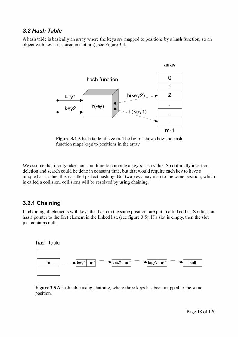
3.2 Hash TableA hash table is basically an array where the keys are mapped to positions by a hash function, so an object with key k is stored in slot h(k), see Figure 3.4.

We assume that it only takes constant time to compute a key´s hash value. So optimally insertion, deletion and search could be done in constant time, but that would require each key to have a unique hash value, this is called perfect hashing. But two keys may map to the same position, which is called a collision, collisions will be resolved by using chaining.

3.2.1 ChainingIn chaining all elements with keys that hash to the same position, are put in a linked list. So this slot has a pointer to the first element in the linked list. (see figure 3.5). If a slot is empty, then the slot just contains null.

of 120

Figure 3.4 A hash table of size m. The figure shows how the hash function maps keys to positions in the array.

h(key)key2

01

2

.

.

.

m-1

hash function

h(key2)

array

h(key1)

key1

Figure 3.5 A hash table using chaining, where three keys has been mapped to the same position.

hash table

key1 key2 key3 null

3.2.2 PerformanceThe performance of chaining strongly depends on the load factor, the load factor is the average number of objects used in a chain.

Our analysis will rely on the assumption, that the hash function evenly distributes the keys in the table. Then the load factor determines the length of chains and thus the running time for insert, delete and search is O(α).

The worst case would be if the size of the table is set to one, then all elements would be stored to the same slot, which would give the same performance as a linked list. The best case under the before mentioned assumption is when α = 1, since no collisions would then occur in the table.

of 120

= nm where n is the number of elements and m is the size of the table.

Definition 3.1 The load factor.

3.3 Inverted IndexAn inverted index is a data structure that maps words or numbers to its location in e.g. a file or document. That is the words in a file are used as keys in the chosen data structure, each of these keys then maps to the files it is a part of. The index is called inverted since the word or number is used to find the file rather than the other way round.

In Table 3.1 are listed three documents and their containing texts. These are indexed into an inverted file index (Table 3.2) and a full inverted index (Table 3.3), the difference between these two indexes is that the full inverted index, also has references to the words´ positions in the text.

Words in a inverted index does not necessarily have to map to a file or document, in this project the keys map to objects instead e.g. a publication object.

Table 3.1 Example of three documents and their containing text.

Document Text1 Introduction to Algorithms2 Where Genetic Algorithms Excel3 Introduction to Artificial Intelligence

Table 3.2 Inverted file index Word Documentintroduction 1,3to 1,3algorithms 1,2where 2genetic 2excel 2artificial 3intelligence 3

Table 3.3 Full inverted indexWord (Document; Position)introduction (1; 1), (3, 1)to (1; 2), (3; 2)algorithms (1; 3), (2; 3)where (2; 1)genetic (2; 2)excel (2; 4)artificial (3; 3)intelligence (3; 4)

of 120

3.4 Binary SearchBinary search is a divide-and-conquer algorithm, that works on lists sorted in ascending order. On each iteration, the algorithm cuts the total search space in half and thus has the search time of O(Log2 n).

The algorithm uses three variables

1. lowThis variable holds the lowest position in the list, in which the search key can reside.

2. highThis variable holds the highest position in the list, in which the search key can reside.

3. midThis variable is the computed middle-position of the interval [low;high]. The value on this position is used for comparison with the search key. If the key is less than the middle-value, then the key must reside in a position lower than the middle-position. If the key is greater than the middle-value, then the key must reside in a position higher than the middle-position. And finally if the key is equal to the middle-value, then the key has been found.

The algorithm returns an integer as the result, if the integer is negative then the key is not in the list and if it is positive then the integer corresponds to the key´s position in the list. Figure 3.6 shows how the binary search algorithm cuts the search space in half after each iteration, further, the three variables low, high and mid are shown for each iteration. Since the key is found in the list, mid is returned as the key´s position. The example also shows that the search time is O(Log2 n).

3.4.1 Inserting into a Sorted ListBinary search can also be used to for finding the insert-position in a sorted list. The search is performed as described above, if the key is not found then the result of Formula 3.1 is returned. The insert-position can then be calculated by using the Formula 3.2. For example if the list in figure 3.6 was searched for the key “i”, then formula 3.1 would return -9. Then using Formula 3.2 the insert-position would be 8, so “i” should be inserted in the end of the list.

of 120

Figure 3.6 A worst-case scenario using the binary search algorithm on a list containing 8 elements. In this example the search is performed with the key “c”.

hgfedcba

dcba

dc

c

low=0, high=7, mid=3

low=0, high=3, mid=1

low=2, high=3, mid = 2

|index = - (low + 1)

Formula 3.1 The index-position

|position = - (index) - 1

Formula 3.2 The insert-position

3.5 Red-Black TreeA red-black tree (RBT) is basically a binary search tree (BST), where each node has a colour attribute. This colour attribute is used to keep the tree balanced.

Each node in the BST has 3 pointers, a pointer to its parent, a pointer to its left child and a pointer to its right child. Besides the pointers each node contains a key and optional satellite data. Nodes in the tree are stored according to the keys, a left child contains a smaller key than its parent and the right child a bigger key than its parent. So all keys in a node´s left subtree must be smaller and all keys in the node´s right subtree must be bigger (see Figure 3.7).

If keys are inserted in ascending or descending order in a BST, then the tree will get the same structure as a linked list and thus the same search time O(n), since the tree´s height h is equal to the number of nodes n (see Figure 3.8).

A RBT keeps the binary tree approximately balanced (no matter in which order keys are inserted) by colouring the nodes either red or black and by using a fixup procedure, that makes sure the properties of a RBT is kept. Therefore the height of the tree is O(log2 n) (see Figure 3.9).

of 120

Figure 3.7 A balanced binary search tree. Keys are inserted in the following order: 4, 2, 1, 3, 6, 5, 7 and 8.

4

71

6

8

5

2

3

Figure 3.8 A binary search tree, where keys are inserted in ascending order.

4

7

1

6

8

5

23

3.5.1 Searching the RBTA search starts from the root node and traverses down the tree until either the key is found or a leaf is reached. At each node a comparison is made and the result of this comparison determines the path.

There are three possibilities

1. The search key is equal to the node´s key; the resulting node is returned and the search is completed.

2. The search key is less than the node´s key; the search algorithm will take the path to the node´s left child.

3. The search key is bigger than the node´s key; the search algorithm will take the path to the node´s right child.

Therefore a worst-case search is when the key is either non-existent or when it is stored deepest in the tree. The search time is therefore O(h), where h is the height of the tree. Since a RBT is always “almost” balanced, the search time is O(log2 n).

3.5.2 Inserting a keyJust like searching the insert procedure starts at the root node and traces a path downward in the tree. When null is reached then the key´s position is found and the pointers are updated to insert the new node.

Searching for the position takes the time O(log2 n), as described in section 3.5.1. The insertion part only takes constant time, as it only requires the pointers to be updated. Since when a node is inserted in the tree, the tree might not be balanced anymore, meaning that the red-black properties might be violated. Therefore the algorithm uses a fix-up procedure that fixes violations by doing rotations and re-colouring. The running time of the fixup-procedure is O(log2 n), since it in worst-case has to take the path all the way up to the root node. The total running for insertion is O(log2 n).

3.5.3 Deleting a keyBefore the deletion can begin, a reference to the node containing the key is needed, the reference can be achieved by performing a search.

of 120

Figure 3.9 A red-black tree, where keys are inserted in ascending order.

4

71

6

8

5

2

3

Deleting in RBTs are done in two steps

• Step1 - the node is removed from the tree.

• Step2 - the fixup procedure is performed.

Step1When deleting the node there are tree cases

1. The node has no children; the node is removed by updating its parents pointer to null.

2. The node has one child; the node is removed by updating its parent´s and its child´s pointers.

3. The node has two children; the node´s successor with no left child is removed and then the successors data is copied into the node to be deleted.

Updating the pointers takes O(1) time, while it in step3 takes O(log2 n) time to find the successor.

Step2The fixup procedure starts at the child of the deleted node and moves the problem up in the tree, the problem is solved at latest at the root. Thus the fixup procedure takes O(log2 n) time.

The total running time is therefore O(log2 n).

of 120

3.6 Ternary Search TreeThe ternary search tree (TST) is a k-ary search tree where k=3 and it is used for storing a set of strings. Each node in the tree has 4 pointers, a pointer to its parent´s node and a pointer to each of its three child nodes, that is its left, middle and right child. Besides the pointers each node contains one character from an indexed key and one value object. If the contained character is not the final character of a key then the value object is null.

The tree is structured by the nodes containing characters, a node´s left child must contain a character lexicographically smaller and the right child must contain a character lexicographically higher. The node ´s middle child contains the next character in an indexed string e.g. if the string “sun” is an indexed key, then “u” could be a middle child of “s” and “n” a middle child of “u”, if and only if the nodes did not already have a middle child, when “sun” was inserted (Figure 3.10).

The TST makes no guarantees of what height the tree will have, the height depends on the keys and in which order they are inserted. In a balanced TST like in Figure 3.10 the height is log3(n) and in the worst-case, the tree is like a linked list (Figure 3.11). Further the TST of Figure 3.10 can be inspected, when keys are inserted in ascending order (Figure 3.12), which is a bit better than the worst case scenario.

of 120

Figure 3.10 A balanced ternary search tree. The TST contains the keys an, be, by, in, is, it, of, on, or and to. Nodes with a bold line symbolises the nodes that contains a non-null value-object, that is the satellite data stored with the associated key.

i

t

s o

e n

b

rf

tn

n y i

ha

o

Figure 3.11 Worst-case scenario of a TST.

i

s

n

t

d

f

Both the best-case and worst-case are highly unlikely when strings are of different lengths and are inserted randomly. Therefore the average height of the tree would be useful, but it has not been possible to find such analysis of the algorithms. Quoting Robert Sedgewick [B2] “We refrain from a precise average-case analysis because TSTs are most useful in practical situations where keys neither are random nor are derived from bizarre worst-case constructions.”.

Therefore further search time analysis will rely on the empirical tests performed in this project.

3.6.1 Searching the TSTStarting at the root node, the algorithm compares the current character in the search string, with the encapsulated character in the node. When starting at the root the first character of the search string is set as the current character. The comparison determines the path the search takes, there are three cases.

1. The search character is lexicographically equal to the node´s character, the search takes the path to the node´s middle child. The current character is found and the next character in the search string is therefore set as the new current character.

2. The search character is lexicographically smaller than node´s character, the search takes the path to the node´s left child.

3. The search character is lexicographically bigger than node´s character, the search takes the path to the node´s right child.

of 120

Figure 3.12 A ternary search tree where the keys are inserted in ascending order. The TST contains the keys an, be, by, in, is, it, of, on, or and to. Nodes with a bold line symbolises the nodes that contains a non-null value-object, that is the satellite data stored with the associated key.

i

t

s

o

e

n

b

r

f

t

n

n

y i

h

a

o

This procedure is continued until either a leaf or the last character in the search string is reached. If the last character in the search string is reached, then the query has been found and the value object of the current node is returned as the result.

The best case search time is when the search string is stored, with its first character in the root node. In this case the search time is the length of the search string.

The worst case search time, is when the last character of the search string is stored in the node furthest down the three, the search time is then the height of the three.

3.6.2 Inserting a keyInserting a key-value pair almost works the same way as the search procedure. The algorithm searches the tree using the key string, if a leaf is reached then nodes are created for the remaining characters in the key. The value object is then stored in the node containing the last character of the key. In case the TST already contains the key, the value objects is overwritten with the new value. This can be avoided e.g. by doing a search for duplicates before inserting. The total insertion time is O(h).

of 120

3.7 SetsIn this section theory on sets which is relevant to this project is described.

A set is a collection of distinct objects, in the following examples integers will be used as objects.

The intersection of two sets A and B is all the distinct elements in A which are also in B, similarly it is also all the element in B which are also in A. In the example in Figure 3.13 the intersection between A and B is the set {23, 41, 56, 87}.

The union of two sets A and B is all the distinct elements which are in either A or B. In the example in Figure 3.14 the union between A and B is the set {1, 2, 3, 7, 9, 23, 41, 54, 56, 87, 122}.

of 120

Figure 3.13 Intersection – The shaded area shows the intersection between the two sets A and B.

Figure 3.14 Union – The shaded area shows the union between the two sets A and B.

4 Basic Part4.1 Index1 – A linked list of linesIn this first step of the project the task is to download and run the provided program Index1. Index1 is a very simple search engine that provides an initial skeleton for the project. Basically it uses a singly linked list as data structure and a search can tell whether an author with a name matching the query exists.

4.1.1 InitializationThe program works by scanning the file line by line. Each line is inserted as satellite data in a singly linked list. An object is inserted into the end of the list by updating the next pointer for the current last object. This gives a structure where the first line in the file is stored in the first object and the last line in the last object. While reading the file, a pointer to the last inserted object is saved, this pointer makes it possible to do the insertion in O(1) time. Insertion has to be done for every line in the file, thus the initialization time is O(L) where L is the number of lines in the file. (see Graph 4.1)

4.1.2 SearchingThe search iterates through the linked list looking for an element which satellite data starts with the string “<author>”, when such an element is found, then the author´s name is extracted from the XML tags and compared to the query. If there is a match, then the query followed by “exists” is printed to the console. In the case that the query can´t be found in any of the author elements, then the query followed by “does not exist” is outputted. The running time for a search is O(L), where L is the number of objects in the linked list, which is the same as the number of lines. (see Graph 4.2)

4.1.3 Space usageEach line in the file is saved as a string in an object in the linked list, so the space usage is proportional with the number of lines. Assuming that a file contains twice as many lines as a file half its size, the space usage is therefore linear. Graph 4.3 shows the measured memory used.

4.1.4 Performance test and analysis

4.1.4.1 Initialization timeThe graph clearly shows the linear behaviour, which reflects the analysed initialization time of O(L).

of 120

4.1.4.2 Search timeIn Graph 4.2 the query time is shown. There are two cases; worst case and best case. In the worst case the query is for a non-existent author, which results in an iteration through the entire linked list. The graph shows the linear growth as the file gets bigger. In the best case the query is for the author located first in the list. This query is extremely fast regardless of the file size, since the author is always located in the beginning of the linked list, the graph clearly shows this constant search time behaviour.

4.1.4.3 Memory usageThe measured memory in Graph 4.3 reflects the linear space usage, where each line in the data file is stored as an element in the linked list.

of 120

Graph 4.2 Index1 - Search time

0 50 100 150 200 2500

50

100

150

200

250

300

350

Index1 - Search time

Worst caseBest case

File size (MB)

Tim

e (m

s)

Graph 4.1 Index1 - initialization time

20 40 60 80 100 120 1400

5

10

15

20

Index1 - Initialization time

File size (MB)

Tim

e (s

)

of 120

Graph 4.3 Index1 – Memory usage

0 50 100 150 200 2500

200400600800

100012001400

Index1 - Memory usage

File size (MB)

Mem

ory

(MB

)

4.2 Index2 – Output an author´s publicationsHere in the 2nd step of the basic part, the task is to update the program to output all the publications by an author, instead of just outputting whether the author exists or not. The data structure is still a linked of lines, the change in this version is in the search procedure.

4.2.1 InitializationThere is no changes to the data structure or the processing of the file. The program still reads the file line by line, while saving each line item in a singly linked list. Hence the time for initialization is still O(L), where L is the number or lines in the XML file. (see Graph 4.4)

4.2.2 SearchingWhen a query is made the linked list is iterated as in Index1, looking for a matching author name. If the name is found then a boolean is set to true, to indicate that the following publication title should be printed to the console. The title is extracted from the XML tags analogously to the extraction of the author name, but by searching the line items for the tag “<title> instead. When a title has been printed the boolean is changed back to false, so the following title will not be printed. The entire list has to be iterated, to make sure that all the publications are found, this is because the authors are listed for each of their publications.

The running time for a search is still O(L), but since the entire list must be iterated every time, the performance will be worse than Index1 for some queries. Index1 could potentially find the author earlier in the list and thus be finished with the query. (see Graph 4.5)

4.2.3 Space usageThe data structure is still a linked list of lines and the space usage is therefore still linear. The tested memory usage is shown in Graph 4.6.


4.2.4.1 Initialization time

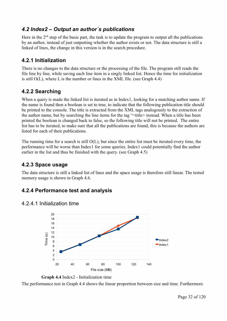
The performance test in Graph 4.4 shows the linear proportion between size and time. Furthermore

of 120

Graph 4.4 Index2 - Initialization time

20 40 60 80 100 120 14002468

101214161820

Index2Index1

File size (MB)

Tim

e (s

)

The graph shows that Index2 still has the same initialization time as index1, as they approximately follow each other.

4.2.4.2 Search timeThe graph shows the described behaviour, as Index2´s search time for all queries matches Index1´s worst case search time.

4.2.4.3 Memory usageThe data structure is still a linked list of lines and therefore the tested memory usage is still linear.

of 120

Graph 4.6 Index2 – Memory usage.

0 50 100 150 200 2500

200

400

600

800

1000

1200

1400


File Size (MB)

Mem

ory

(MB

)

Graph 4.5 Index2 - Search time.

0 50 100 150 200 2500

50

100

150

200

250

300

350

400

Index2Index1 – w orst caseIndex1 – best case

File size (MB)

Tim

e (m

s)

4.3 Index3 – Linked list of authors and their publicationsThe task in Index3 is to change the data structure from a linked list of lines to a linked list of authors and for each author have a reference to the author´s linked list of publications.

Figure 4.1 shows the new program structure, satellite data not relevant for the program structure has been omitted from the objects. Author objects are denoted by an A and publications by a P, the number following the denotation is only to show that they are different objects. Each author element now has a reference “start” to the beginning of their linked list of publications.

Note that a publication can have several authors and is therefore listed once for each of the authors. This can be seen in Figure 4.1, where the publication object P2 is listed in both A1 and A2´s lists. To be more precise, when a publication is represented in several linked lists, it is only the publication object that must be created several time, the title string is only created once, each publication thus has a reference to the same string.

4.3.1 InitializationThe new data structure means that the way the file is parsed is changed. The file is still read line by line, searching for an author tag. When an author is found, it is known from the structure of the XML, that all the authors of the current publication will follow. So the algorithm will save each author for a publication in a temporary linked list, and for each of these authors search the entire linked list of authors for duplicates. When an author object is already in the list, then the object is updated with the publication, in this case the author´s list of publications is searched for duplicates. So the search for duplicate authors will be performed for every author tag in the file. The search will take more and more time as the author objects are added, since the list grows bigger. The total time is therefore the sum of searches, which can be described by the formula shown in Figure 4.2. Adding publications is done in linear time, since the search for duplicates only is performed on the specific author´s list of publications, the search is therefore seen as running in constant time.

of 120

Figure 4.1 The data structure used in Index3, showing a linked list of authors {A1, A2, A3} and each author´s respective linked list of publications. Publications in the illustration is {P1, P2, P3, P4, P5}.

A1

P1

start

P2

P3

start

null

A2 A3

P2

null

start

P4

P5

null

null

start

The initialization thus has the quadratic running time O(A2), where A is the total number of authors in the file. (see Graph 4.7)

4.3.2 SearchingTo find an author, the linked list must be iterated. This takes O(A) time, where A is the number of authors in the list. An improvement in search time is expected as as the linked list now only contain authors, whereas Index1 and Index2 stored all the lines in file. (see Graph 4.8)

4.3.3 Space usageIndex3 uses a linked list of unique authors, where each author has a linked list of publications. That means that the same publication must be added as an object for each of its authors. Assuming that the number of publications is somewhat evenly distributed among the authors, the space usage is linear. (see Graph 4.9)


4.3.4.1 Initialization timeThe performance test shows the quadratic behaviour of the initialization time.

of 120

Figure 4.2 Summation formula, for calculating Index3´s initialization time.

Graph 4.7 Index3 - initialization time. The computed equation for the graph y = 0,2593x2 + 1,0791x.

0 20 40 60 80 100 120 140 1600

1000

2000

3000

4000

5000

6000

7000


File size (MB)

Tim

e (s

)( ) 2 2

1

1 1 112 2 2

A

ii A A A

=

= + − − =∑

4.3.4.2 Search timeThe worst case search time for Index3 in Graph 4.8 nicely follows the analysed linear search time. Graph 4.9 further shows the improvement in search time compared to Index1 and Index2, the reason is, that now the length of the list is the number of unique authors in the file, whereas before the list contained all the lines from the file.

4.3.4.3 Memory usageThe measured memory usage can be seen in Graph 4.10, which shows the linear growth in memory.

of 120

Graph 4.9 Index3 – Search time comparison with Index1 and Index2.

0 20 40 60 80 100 120 140 1600

50

100

150

200

250

300

Search time

Index3 – Worst caseIndex2Index1 – w orst case

File size (MB)

Tim

e (m

s)

Graph 4.8 Index3 – Search time.

0 20 40 60 80 100 120 140 1600

5

10

15

20

25

30

35

40


Index3 – Worst caseIndex3 – Best case

File size (MB)

Tim

e (m

s)

In Graph 4.11 Index3 is compared to Index1 and Index2, the improvement in space usage is clearly shown. The reason for this is because Index3´s linked list only contains the number of unique authors, whereas Index1 and Index2´s contains all the lines from the XML file. Even though Index3 also has a linked list of publications for each author, the memory is still reduced significantly.

of 120


0 20 40 60 80 100 120 140 1600

20406080

100120140160180


File size (MB)

Mem

ory

(MB

)

Graph 4.11 Index3 - Memory usage. Comparison with Index1 and Index2.

0 20 40 60 80 100 120 140 1600

200

400

600

800

1000

1200

Index3Index1 & Index2

File size (MB)

Mem

ory

(MB

)

4.4 Index4 – Hash tableIn this final step of the basic part, the task is to modify the data structure to use a hash table (see section 3.2) to store the author objects.

Figure 4.2 shows the modified data structure. The structure of the linked lists is the same as in Index3 (see section 4.3), but instead of having one huge linked list of author objects, the authors are now distributed among the hash table and thus the linked list of authors only contains more than one object if there is a collision.

The authors´ names are used as the keys in the table. The keys are hashed to the table by using the method described by formula 4.1.

The function hashCode in the formula is Java´s hashcode method, which converts the string into an integer. The numeric value of this integer is then computed to make sure the integer is positive. And finally modulus is used with the size of the hash table, to distribute the integer to a position within the right range.

of 120

Figure 4.2 The data structure used in Index4 – A hash table using chaining to store the author objects. The figure shows three author objects and their linked lists of publications, the authors have been hashed to the same position in the table and stored in a linked list.

A1

P1

start

P2

P3

null

A2 A3

P2

null

start

P4

P5

null

null

start

Hash table

|hashCode(key)| mod tableSize

Formula 4.1 The hash function

4.4.1 InitializationThe algorithm used to parse authors and their publications is still the same as in Index3 (see section 4.3.1). But the time it takes to search, delete and insert has been greatly improved with the hash table. Assuming that the hash function can be computed in constant time, a search can be performed in O(α) time, where α is the number of author objects in a chain (Definition 3.1 - the load factor). In the implementation the size of the hash table is set, to keep the load factor below 1, to aim for a constant running time. The total initialization time is therefore O(A *α ), where A is the number of authors in the XML file. (Graph 4.12)

4.4.2 SearchingTo find an author, the query is mapped to the table using the hash function and then the linked list of authors in that position is iterated. Still under the assumption that the hash function takes constant time, the time for a search then depends on the size of the linked list. So the time for a search is O(α), where α is the number of elements in the chain. The implementation is made such that the capacity of the table, is set to aim for a 75% load factor, this is also the default load factor in Java Sun´s implementation and should offer a good trade-off between time and space. Therefore as α is below 1, we get the constant running time O(1). (Graph 4.15)

4.4.3 Space usageThe space usage should not have changed much compared to Index3, both applications have an object for each unique author and a linked list of publications for each of the authors. The only difference is, that now the author objects are stored in a hash table using chaining, instead of in a linked list. Therefore a linear increase in space usage is expected as more data is parsed into the data structure (See Graph 4.17).


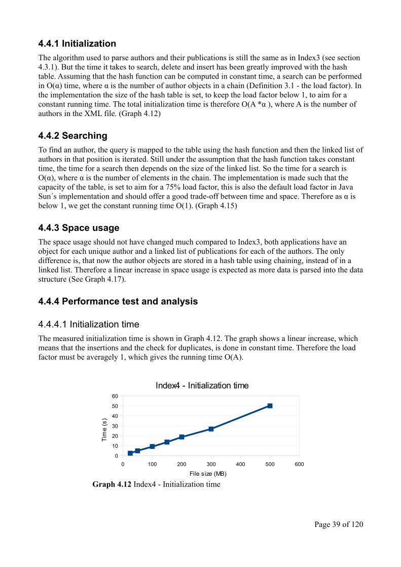
4.4.4.1 Initialization timeThe measured initialization time is shown in Graph 4.12. The graph shows a linear increase, which means that the insertions and the check for duplicates, is done in constant time. Therefore the load factor must be averagely 1, which gives the running time O(A).

of 120

Graph 4.12 Index4 - Initialization time

0 100 200 300 400 500 6000

10

20

30

40

50

60


File size (MB)

Tim

e (s

)

The initialization time has been greatly improved compared to Index3, which ran in quadratic time (see Graph 4.13). This is because of the check for duplicates, where the hash table can perform a search in constant time (see 4.4.2 Searching) and Index3 in linear time. Index4 also has faster initialization time than Index1 and Index2 (see Graph 4.14), the reason is that Index4 only stores the authors and their publications, where Index1 and Index2 store all the lines from the XML file.

4.4.4.2 Search timeGraph 4.15 shows the measured search time. The queries were so fast that they had to be measured in nanoseconds to get a result. So even though the graph seems to “jump”, the time range is so small, that a reliable conclusion, that queries for one file size is faster than another cannot be made. But the test gives an indication of the queries time range, and it clearly shows that a search can be performed in O(1) time.

The constant query time is a great improvement compared to the previous versions, Graph 4.16 shows the difference. Now the search time is approximately as fast as the best case search in index3.

of 120

Graph 4.15 Index4 – Search time.

0 100 200 300 400 500 600 700 8000

0,01

0,01

0,02

0,02

0,03


File size (MB)

Tim

e (m

s)

Graph 4.13 Index4 - Initialization time comparison with Index3.

0 20 40 60 80 1001201401600

1000

200030004000

50006000

7000

Initialization time

Index4Index3

File size (MB)

Tim

e (s

)

Graph 4.14 Index4 - Initialization time comparison with Index1 and Index2.

0 20 40 60 80 1001201401600

5

10

15

20

Initialization time

Index4Index1 & Index2

File size (MB)Ti

me

(s)

4.4.4.3 Memory usageThe measured memory usage shows the linear increase in memory as more data is loaded into the data structure.

When comparing the memory usage with Index3, the graphs roughly follow each other. Index4 takes slightly more space, due to the added array containing the author objects.

of 120

Graph 4.16 Index4 – Memory usage comparison with Index3.0 20 40 60 80 100 120 140 160

020406080

100120140160180200

Index4Index3


0 100 200 300 400 500 600 700 8000

100200300400500600700800900


File size (MB)

Mem

ory

(MB

)

Graph 4.16 Index4 – Search time comparison with Index3.

0 20 40 60 80 100 120 140 1600

5

10

15

20

25

30

35

40

Index4Index3 – Worst caseIndex3 – Best case

File size (MB)

Tim

e (m

s)

5 Advanced Part5.1 Index5 - Title SearchIn Index4 it was only possible to search for authors, so this first update in the advanced part will be to support searching for publications as well. Just as a search for an author would output all titles written by the author, so shall the application now output all authors of the specified publication.

Figure 5.1 shows the modified data structure, the only change is that now the application contains two hash tables, a hash table for the authors as in Index4 and a hash table for publications. The title of the publication is used to hash it to the table and each publication contains a linked list of its authors.

5.1.1 InitializationThe algorithm for reading the file has not been modified, all authors for a read publication are still kept in a temporary linked list. Now when a title is read the publication is added (with duplication check) with the temporary list of authors, as its linked list. Afterwards the temporary list is iterated and the authors are added or updated one by one with the publication, as in Index4.

Index5 has a linear initialization time, since it takes constant time to add an object to either of the hash tables. The only difference from Index4, is that now we have to add all the objects twice. This does not mean that the gradient is doubled, the reason is the way objects are added to the two hash tables. When adding to the authors table, the temporary list of authors needs to be iterated, to add the publication for each author, but when adding to the publications table, a publication can be added in one step, as the temporary list contains all the authors of the publication. Therefore the running time is still linear, but with a bit more steep gradient (See Graph 5.1).

5.1.2 SearchingA search in a hash table still takes O(α), where α is the number of objects in the chain. In Index4 it was shown that the implementation provides constant time lookup in the hash table (see section 4.4.2). In Index5 there are two hash tables, therefore when a query is made a search is performed on both hash tables. Thus the search time is still O(1), but the constant should be approximately twice the size (See Graph 5.2).

of 120

Figure 5.1 Data structure of Index5. Publication objects is denoted by the prefix P and author objects by the prefix A.

A1

P1

start

P2

P3

null

A2 A3

P2

null

start

P4

P5

null

null

start

Hash table<String name, Author a> authors

P1

A1

start

A2

A3

null

P2 P3

A2

null

start

A4

A5

null

null

start

Hash table<String title, Publication p> publications

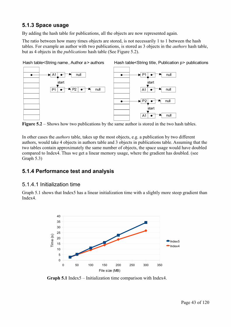
5.1.3 Space usageBy adding the hash table for publications, all the objects are now represented again.

The ratio between how many times objects are stored, is not necessarily 1 to 1 between the hash tables. For example an author with two publications, is stored as 3 objects in the authors hash table, but as 4 objects in the publications hash table (See Figure 5.2).

In other cases the authors table, takes up the most objects, e.g. a publication by two different authors, would take 4 objects in authors table and 3 objects in publications table. Assuming that the two tables contain approximately the same number of objects, the space usage would have doubled compared to Index4. Thus we get a linear memory usage, where the gradient has doubled. (see Graph 5.3)


5.1.4.1 Initialization timeGraph 5.1 shows that Index5 has a linear initialization time with a slightly more steep gradient than Index4.

of 120

Figure 5.2 – Shows how two publications by the same author is stored in the two hash tables.

A1

P1

start

P2

null

null

P1

A1

start

null

null

P2 null

start

A1 null

Hash table<String name, Author a> authors Hash table<String title, Publication p> publications

Graph 5.1 Index5 – Initialization time comparison with Index4.

0 50 100 150 200 250 300 3500

5

10

15

20

25

30

35

40

Index5Index4

File size (MB)

Tim

e (s

)

5.1.4.2 Search timeThe measured search time still shows that a query can be performed in constant time. FurthermoreIn Graph 5.2 the comparison shows, that queries on Index4 is only faster in 4 out of the 6 cases. This is due to the extremely fast query time, which makes it hard to get the precise difference between Index4 and Index5.

5.1.4.3 Memory usageIndex5´s memory usage is still linear with the size of the data file (see Graph 5.3). Furthermore by using the graphs´ calculated functions the difference in the gradients can be found. Index5´s gradient is approximately ((2,003/1,0399) ≈ 1,93) 193% the size of Index4´s gradient, thus the added hash table of publications must contain less objects than the hash table of authors.

of 120

Graph 5.3 Index5 – Memory usage comparison with Index4.The computed functions: Index5: yindex5=2,003x and Index4: yindex4 = 1,0399x

0 50 100 150 200 250 300 3500

100

200

300

400

500

600

700

Index5Index4

File size (MB)

Mem

ory

(MB

)

Graph 5.2 Index5 – Search time comparison with Index4.

0 50 100 150 200 250 300 3500

0,01

0,01

0,02

0,02

0,03

Index5Index4

File size (MB)

Tim

e (m

s)

5.2 Index6 - Keyword SearchSo far it has only been possible to get a search result, if an exact author name or publication title is used. This does not provide a very good search engine, therefore in this increment, the application is updated to support queries for keywords. The concept is that publications and authors can be found by searching for a word that their title or name contains.

Index6 is implemented as an inverted index (see section 3.3), where each word refers to all the titles or names, that it is a part of. Hash tables using chaining are still used, now they just store the words instead of titles and names, that is the words are hashed into the hash table instead. There is a hash table for words which refers to publications and a hash table with words that refers to authors (See Figure 5.3). As shown in the figure, two new types of objects are added, that is the name and keyword objects. These objects are used to store the words in names and titles accordingly, as well as they are used in a linked list in case of collisions in the hash table. Furthermore each name object has a linked list of author objects and each keyword object has a linked list of publication objects.

To improve the search engine further, a filter removing words with “no search value” has been implemented. This is done for both titles and author names, but it is done in two different ways. For filtering words in a title, a list of stop words is used. Stop words are words that does not add meaning to a title e.g. “the”, “to” and, “in” and thus not give meaning as a query (unless used in a sentence). Stop words must be used with care, to avoid that certain titles cannot be found. The stop words are hand picked, with inspiration from a list of common English stop words [I5]. All of the used stop words can be found in the appendix in section 10.3.

Besides stop words a few conditions are used, the complete filter is defined by the terms keyword and namepart. All words in a title which are not removed by the filter are defined as a keyword (Definition 5.1), and all “words” in a name, which are not filtered are called a namepart (Definition 5.2).

of 120

Figure 5.3 Index6 - Data structure. Two new classes are added to application Name and Keyword. Name objects are denoted by the prefix N and keyword objects by the prefix K. Publication and author objects are still denoted by the prefix P and A accordingly.

K1

start

K2 K3 null

Hash table<String keyword, Keyword k> keywords

P1 P2 P3 null

A1 A2 A3 null

start

Hash table<String namePart , Name n> names

N1

start

N2 N3 null

A1 A2 A3 null

P1 P2 P3 null

start

null

start

null

start

null

startnull

start

null

start

null

start

5.2.1 InitializationThe algorithm for parsing the file into data structure has been slightly changed, the modifications has been made to the way names and titles are added.

• When a title tag has been read and the publication object created, then the title is split into words and each word is tested if it is a keyword. If the word is a keyword, then it is added to the hash table and the publication is added to the keyword object´s linked list of publications (both keyword and publication are added with duplication check) .

• When the temporary list of author names for the publication is iterated, then an author object is created on each iteration, and the author name is split into words. Each word is tested if it is a namepart, if the word is a namepart, then it is added to the hash table and the author object is added to the namepart´s linked list of authors (both the namepart and the author are added with duplication check).

This will result in an increased initialization time, now each factor contributing to the running time will be analysed. The following list is for every time a publication or author is parsed from the file.

• Iterating through all the words in a title / name.Each title consists of 1 to 43 words, but the calculated average is 8 words per title (including stop words). Author names consist of even less words, in most cases 2-3 words. Therefore iterating the titles or names will be seen as a constant.

• Testing if word is a keyword / namepart.The filter for the names takes constant time, as it only needs to check for the two conditions (Definition 5.2). The filter for the titles, also needs to search the list of stop words. The stop word list is implemented as a sorted list, this way a binary search (see section 3.4) can be performed, which has a running time of O(lg2 n). The list contains 89 stop words, and thus testing if a word is a stop word takes ( lg2 89 ≈ 6,5 ) at most 7 comparisons. Therefore searching the stop word list will be seen as a constant.

of 120

A keyword is a word in a publication title, which satisfies both of the following conditions.

• The word has a minimum length of 2 characters.

• The word is not a stop word.

Definition 5.1 Keyword

A namepart is a word in an author name, which satisfies both of the following conditions.

• The word has a minimum length of 2 characters.

• If the word has a length of 2 characters, then the word may not end with a “.” (period).

Definition 5.2 Namepart

• Inserting keyword / namepart.Before an insertion, the hash table is searched for duplicates, this is done in constants time. Searching is further elaborated in section 5.2.2.

• Inserting the publication in the keyword´s linked list of publications / inserting the author in the namepart´s linked list of authors.Before the insertion the linked list must be searched for duplicates, the worst case search time is thus the the number of elements in the list (section 3.1.1). This list can in some cases be quite long, since the linked list for e.g. a keyword contains all publications, that include that keyword. The filter therefore also improves the initialization time (see Graph 5.5), as the linked lists for the filtered words grow very large.

The number of elements in a linked list, was tested using the keyword “algorithm” and the namepart “Michael”. Using the 25MB file the query “algorithm” returned 2025 unique publications and the query “Michael” returned 921 unique authors. For the 100MB file the result was 6824 publications and 2421 authors. From the small test it can be seen, that the lists grow bigger as more data is parsed.

Therefore inserting a publication has a running time of O(p) and inserting an author has the running time O(a), where p is the size of the list of publications for the keyword and a is the size of the list of authors for the namepart.

As it takes linear time to parse the publications and the authors, and also linear time to search the lists for duplicates, the total initialization time is quadratic (see Graph 5.4). The initialization time can be expressed with O(p ∙ P + a ∙ A), where p is the number of publications in the file and a is the number of authors in the file.

5.2.2 SearchingA search in a hash table still takes O(α), where α is the number of objects in the chain. In Index4 we showed that the implementation provides constant time lookup in the hash table (see section 4.4.2).Like in Index5 there are two hash tables, therefore when a query is made a search is performed on both hash tables. Thus the search time is still O(1) (see Graph 5.6).

In the previous versions of the application, an exact title or name in a query was required to get a result, and thus there would only be one result returned on a successful query. Here in Index6, when a query is successful, there can be several results. A successful search in Index6 returns the first object in the linked list of results. As illustrated in Figure 5.3, e.g. a keyword object has a linked list of publications, this list thus contains the search results for the keyword. The list must be iterated to return all these results to the user. The iteration takes linear time, O(K) for a match on a keyword and O(N) for a match on a namepart.

5.2.3 Space usageThe space usage is still linear with the amount of parsed data, the only difference is that more space is used than in Index5, since now all keywords and nameparts are indexed in the hash tables. This implementation also causes author and publication objects to be represented more times. Graph 5.7 shows the measured memory usage.

of 120


5.2.4.1 Initialization timeGraph 5.4 shows that the measured initialization time nicely follows a quadratic function, this was expected from the analysed time O(p ∙ P + a ∙ A). The graph gets the quadratic behaviour because of the duplication check, when inserting authors and publications in the linked lists. Even though the function is quadratic, it is still quite fast for a 2nd degree polynomial - notice the calculated equation in Graph 5.4. The reason is, when searching for duplicates, it only has to search a small percentage of the total number of publications/authors. Therefore the time O(P2 + A2) would be quite misguiding, even though it is possible to manipulate the data to create this running time. That time could be archived if e.g. all titles had a keyword in common, thus that keyword would have a linked list of all the publications. This scenario is not realistic in practice, especially not with the implemented filter. A test is made where the filter is disabled to see how it affects the performance (see Graph 5.5).

Graph 5.5 clearly shows that when not using the filter, the initialization time is quite higher. This is because the linked lists for common words as e.g. “the”, “for” and “a” grow very large and hence increase the search time. But it is still nowhere near the aforementioned worst case scenario, this can be verified by comparing with Index3 that has the running time O(A2). The measured performance shows that Index3 has by far the worst initialization time. This makes sense as Index3 has to iterate a linked list containing all the authors on every search.

of 120

Graph 5.4 Index6 - Initialization time. The computed equation for the graph y = 0,0064x2 – 0,0237x.

0 50 100 150 200 250 300 3500

100

200

300

400

500

600


File size (MB)

Tim

e (s

)

5.2.4.2 Search timeThe time it takes to process the query and find the result in the hash tables, still runs in constant time. The only change compared to Index5, is that now the hash tables contain more objects, but the size of the hash tables are set such that the load factor is approximately the same. Graph 5.6 shows the similarity in search time.

of 120

Graph 5.6 Index6 - Search time comparison with Index5.

0 50 100 150 200 250 300 3500

0,01

0,01

0,02

0,02

Index6Index5

File size (MB)

Tim

e (m

s)

Graph 5.5 Initialization time comparison. The computed equation for Index6 without the stop word filter y = 0,0523x2 +1,1304x. And the computed equation for Index3 y = 0,2593x2 + 1,0791x.

0 50 100 150 200 250 300 3500

1000

2000

3000

4000

5000

6000

7000

Initialization time

Index6Index6 – Without stopw ord f ilterIndex3

File size (MB)

Tim

e (s

)

5.2.4.3 Memory usageThe performance test shows the linear increase in memory usage and that Index6 now uses more memory than in Index5. This was expected, as the application now stores all the keywords and nameparts and not just the titles and the full names. Another factor that causes the extra memory usage is, that publication and author objects are represented several times more e.g. a publication is stored in each of its keyword´s linked lists.

Graph 5.7 also shows the reduced memory consumption with the implemented filter, that is by using the filter the implementation uses less than half the memory than without the filter. Furthermore using the calculated functions the difference in the gradients can be calculated, Index6´s gradient is ((2,003/4,4024) ≈ 0,46) 46% the size of Index6 without the filter.

of 120

Graph 5.7 Index6 – Memory usage. Memory usage comparison with Index6 - without the stop word filter and with Index5. The graphs´ calculated functions: Index6: y = 3,5395x, Index6-without filter: y = 4,4024x, and Index5: y = 2,003x.

0 50 100 150 200 250 300 3500

200

400

600

800

1000

1200

1400

Index6Index5Index6 – Without stopw ord f ilter

5.3 Index7 - Prefix Search (Auto-suggest)In this section the data structure will be updated to support prefix searches.

Index7 will be implemented using three different data structures, based on the performance tests the most efficient data structure will be used in the next program update. The implementations are a sorted list, a ternary search tree and a red-black tree. Furthermore in the research of finding data structures that supports the desired auto-suggest feature, a suffix tree and a trie was also considered. The suffix tree was not used since it seemed to be overdoing the task, that is the suffix tree is able to find all patterns within a text, but that does not necessarily give the best search results e.g. the query “gor” is a pattern in the word “algorithm” and that is most likely not what the user was searching for. The TST was chosen instead of the trie, since it seemed more interesting and as an improved version of the trie [I9].

The three implementations will still be using the inverted index as in Index6, just as well as the internal structure of publications and authors will remain the same. The only difference will be that the hash tables that store the keywords (Definition 5.1) and nameparts (Definition 5.2) will be exchanged with the aforementioned data structures.

Before continuing with the data structures, the meaning of the prefix search will be further elaborated. The idea is to be able to return a list of results while the user is typing, but the results should not be a list of words which starts with the query. Instead the results should provide a list of authors and publications see Figure 5.4.

When a prefix search is made, a search is performed on the chosen data structure. The search will find the keywords and the nameparts, that start with the prefix. Each of these objects contains a linked list of either authors or publications, these lists combined are the result to the prefix search. This approach also makes it possible to find results, no matter where the word containing the prefix is placed in e.g. a publication title. As Figure 5.4 shows, the query “alg” matches the last word in the publication “Introduction to Algorithms” and it matches the first word in “Algorithm Design”. Another thing to notice in the figure is that a keyword or namepart can have references to several objects, for example the keyword “algorithm” has three publications in its list.

of 120

Figure 5.4 The prefix search. The example shows the auto-suggestions of authors and publications, given the query “alg”.

B. AlgayresV. Ralph AlgaziAnne E. AlgerAlgirdas Avizienis

Algorithm DesignAn Algorithm for Convex Polytopes.An Efficient Algorithm for Graph Isomorphism.

”alg”

Query

keywords

namepartsalgayresalgazialgeralg irdas

algorithm

authors

publications

{An Algebra of Data Flows.

Introduction to Algorithms

algebra

algorithms

5.3.1 Sorted ListThe data structure for this implementation is almost the same as in Index6, where there were two hash tables, one to store the nameparts and one to store the keywords, now the hash tables has just been exchanged with sorted arrays. As there are no collisions in the arrays as there where in the hash tables, there is no longer linked lists of name and keyword objects, therefore these pointers have been removed from the objects. Figure 5.5 shows the data structure; the DynamicArray is a modifed version of Java´s ArrayList, the main difference is that the DynamicArray increases its capacity by a factor 2, when all slots are filled. This provides a good trade-off between time and space usage.

Since this sorted list stores objects and not strings, the modified version of Java´s binary search method has been implemented. The binary search algorithm will search the list by using the string stored within the object, that is the string word for the keyword object and the string namePart for the name object. The lists are kept sorted also by using the binary search algorithm, this way the lists are still in ascending order after each insertion. When the lists are kept sorted they can be searched in O(log2 n), and since binary search returns a negative value if the string is not found and a positive value if is found, then only one search is needed, to both check for duplicates or get the insert-position. (see section 3.4 for the binary search theory).

of 120

Figure 5.5 The data structure of Index7 using a Sorted List. For clarity the internal structure is only shown for one position in each of the lists.

DynamicArray<String keyword, Keyword k> keywords

P1 P2 P3 null

A1 A2 A3 null

start

DynamicArray<String namePart , Name n> names

A1 A2 A3 null

P1 P2 P3 null

start

null

start

null

start

null

start

null

start

null

start

null

start

N1start

K1start

5.3.1.1 InitializationThe most significant change compared to Index6, is that searching for duplicate keywords and nameparts, no longer can be done in O(1) time as with the hash table. The other big change is the time it takes to keep the list sorted. Therefore an increase in initialization time is expected.

There has been no changes in how the file is parsed, therefore several parts of the analysis in section 5.2.1 can still be used. In the following analysis, the descriptions for the parts already described in section 5.2.1, will only summarize the part´s running time. As mentioned above two sorted lists are used to store the objects, the following description will apply to both lists. Each factor contributing to the total running time will be analysed. The following list is for every time a publication or an author is parsed from the file.

• Iterating through all the words in a title / name. O(1)

• Testing if word is a keyword / namepart. O(1)

• Searching the sorted listSearching the list for duplicates (keywords / nameparts) takes O(log2 n) time using binary search (See the theory in section 3.4). If the element is not in the list, then the returned index value is used to calculate the position in the array to insert the object, while still maintaining the ascending order. Thus the running time for searching the list of keywords is O(log2 K) and O(log2 N) for the list of nameparts.

• Inserting keyword / namepart.The search procedure described above provides the position where the object must be inserted. Inserting an element into a list only takes constant time, but since the position to insert the element, usually is not in the end of the list, all elements in the list from the insert-position must be moved 1 position, to make room for the the new object. In worst case that is all the elements in the list. Therefore this part takes O(K) time for the keyword list and O(N) time for the namepart list.

Another factor is when the list is full and needs to be expanded, then the list must be reallocated with a larger size, and all the objects from the original list must be copied into the new and larger list. In the implementation of the DynamicArray, the expansion factor is set to a factor 2, that is the list will have twice as many slots as the old list. By using this expansion heuristic, the amortized cost of an insertion is O(1) [B1].

• Inserting the publication in the keyword´s linked list of publications / inserting the author in the namepart´s linked list of authors. (With duplicates check)Inserting a publication has a running time of O(p) and inserting an author has the running time O(a), where p is the size of the list of publications for the keyword and a is the size of the list of authors for the namepart.

The total running time for the initialization can be expressed by O(P(log2(K) + K + p) + A(log2(N) + N + a)). As it takes linear time to parse the publications and the authors, and the strongest factor inside the parenthesis is also linear, the total initialization time is expected to have a quadratic behaviour. (see Graph 5.8)

of 120

5.3.1.2 Searching5.3.1.2.1 Full searchSearching a sorted list takes O(log2 n) time using the binary search procedure described in section 3.4. When a query is found the position of the string is returned as the result. The element stored in that position is either a keyword or a name object , the element contains the internal structure of linked lists of authors and publications.(Figure 5.5). So to present the results to the user, the element´s linked list must be iterated, for instance if the query was the string “algorithm” then the linked list would consist of all the publications containing the keyword “algorithm”. Iterating through a linked list takes linear time O(n).

The total time for a full search is therefore O(log2(K) + p) when searching for publications and O(log2(N) + a) when searching for authors. (see graph 5.9)

5.3.1.2.2 The prefix searchSearching a sorted list takes O(log2 n) time using the binary search algorithm. The same search procedure can be used for prefix searching. This is done in the following way. When a query is made the binary search method returns an index-value. No matter if the query is found or not, the procedure is basically the same. Usually a prefix is not found, as there are no matches when a search string is a non-completed word. Since the list is sorted in ascending order, we know that the returned index-value or the calculated index-position, is a position in the list where all the following elements are lexicographically bigger than the query.

So our result to the prefix search is all the following positions in the list, which containing objects key starts with the prefix. To avoid comparing if each string in the list starts with query, a second binary search is performed. This search uses an upper bound, so that all elements between the first and the second binary search, must start with the prefix. The string used as the upper bound is set by concatenating the lexicographically biggest character to the search string. The biggest character in our alphabet is the one with highest value in ASCII code, which is “ÿ“ with the code 255. In the case where there is no results, then the second search will return a lower insert-position, such that there is no interval.

As described in the beginning, it is the titles and names that are to be returned as result on a prefix search. Therefore the results to return are in the objects linked lists (see Fig 5.5), that is the linked lists of publications for the found keyword objects and the linked lists of authors for the found name objects. Since there can be a huge amount of results, especially if the query is just one character, a maximum to the number of results is made. This also saves time, as the procedure is ended as soon as the maximum is reached. The maximum will be seen as a constant factor, as there is no reason for that many auto-suggestions(the default value is 20). Therefore the total prefix search time is O(log2 n). That is O(log2K) when searching for publications and O(log2N) when searching for authors. (see Graph 5.10)

5.3.1.3 Space usageThe external data structure consists of two sorted lists, these are implemented using the aforementioned DynamicArray, that increases size by a factor 2 when full. The inner structure of linked lists of authors and publications (see Fig 5.5), are exactly the same as in the previous index (see Fig 5.3). Furthermore the number of each object type is also exactly the same, as there is no change in the way the data is parsed into the data structure.

of 120

The most significant changes in Index7 using sorted lists compared to Index6, when it comes to space usage are

• The removed pointers in the keyword and name objects, as the sorted list does not have any collisions.

• The size of the sorted lists; the lists grow by a factor 2, which can result in empty slots, in worst case only half of the list is full. This happens when no elements are inserted after the last expansions. In the hash table implementation in Index6, the size of the table was set on initialization based on the file size.

Therefore the space usage for the sorted lists is still linear with the amount of parsed data. The removed pointers should give a decrease in space usage and the list expansion might cause an increase in space usage compared to Index6 (See Graph 5.11).

of 120

5.3.2 Ternary Search TreeThe ternary search tree(TST) used is a modified version of Wally Flint´s implementation posted on JavaWorld [I10]. The implementation is based on the algorithms by Jon Bentley and Bob Segdewick [I9]. See section 3.6 for the theory on TSTs.

The internal structure of linked lists remains the same as in Index6. The external structure though has been changed from two hash tables to two TSTs (see Figure 5.6). Looking at the external structure, it is worth noticing that there is no longer any need for the keyword and name objects, as there is no collisions in a TST. Instead the TST uses nodes to store the key-value pairs. This way each key(namepart / keyword) is mapped to a value-object (author / publication object).

5.3.2.1 InitializationThere has been no changes in how the file is parsed, therefore several parts of the analysis in section 5.2.1 remain the same. In the following analysis, the descriptions for the parts already described in section 5.2.1, will only summarize the part´s running time. Each factor contributing to the total running time will be analysed. The following list is for every time a publication or an author is

of 120

Figure 5.6 The data structure of Index7 using the Ternary Search Tree. All nodes in the TSTs contain a character, which is denoted by the prefix “C”. Nodes with a shaded background are nodes that have a non-null value object. The example shows the internal structure of a non-null value object in the two TSTs keywords and names. In this example the value objects is shown for the keyword that consists of the characters C1, C4, C5 and C6 and for the namepart that consists of the characters C1, C4 and C5.

C1

C7 C4C2

C5

C6

C3

P1 P2 P3 null

A1 A2 A3 null

start

null

start

null

start

null

start

TernarySearchTree<String keyword, Publication p> keywords

C8

C1

C7

C4C2

C5C3

TernarySearchTree<String namepart, Author a> names

C6

A1 A2 A3 null

P1 P2 P3 null

start

null

start

null

start

null

start

parsed from the file.



• Inserting keyword / namepart.Before inserting the key-value pair the TST must be searched for duplicate keys (keywords / nameparts). If the element was not in the TST, then the element can be inserted. It is known from the theory, that both a search and an insertion can be done in O(log3n) time, if the tree are balanced and in O(n) time in the worst case (See section 3.6). None of these running times are realistic for the used data in this project and will therefore not be beneficial to the analysis. Therefore the variables “x” and “y” will be used to denote the search/insertion time; x will be used for the TST containing keywords and y for the TST containing nameparts. The performance tests can then give an indication of which function x and y are.

• Inserting the publication in the keyword´s linked list of publications / inserting the author in the namepart´s linked list of authors.Inserting a publication has a running time of O(p) and inserting an author has the running time O(a), where p is the size of the list of publications for the keyword and a is the size of the list of authors for the namepart.

The total running time for the initialization can be expressed by O(P(x+p) + A(y+a)). (see Graph 5.8)

5.3.2.2 Searching5.3.2.2.1 Full searchWhen searching the TST for a key a value-object is returned as the result, if nothing was found then the value-object is null. This value-object objects contains the internal structure of linked lists of authors or publications. So to return all the results to the user the value-object´s linked list must be iterated, for instance if the query was the string “algorithm” then the linked list would consist of all the publications containing the keyword “algorithm”. Iterating though a linked list takes linear time O(n).

As mentioned in section 3.6, the average height of a TST is not known. Only the height is known when the tree is completely balanced (h = log3n) or when in its stretched out like a linked list (h = n). None of these heights are realistic for the used data in this project and will therefore not be beneficial to the search time analysis. Instead the TST will be analysed based on the performance tests, by comparing to the other data structures.

Therefore the former mentioned variables “x” and “y” will be used to denote the search time; x will be used for the TST containing keywords and y for the TST containing the nameparts.

The total time for a full search is therefore O(x + p) when searching for publications and O(y + a) when searching for authors. (see Graph 5.9)

5.3.2.2.2 The prefix searchThe prefix search works similarly to a normal search, for each character in the search string, the algorithm will move down in the tree, by following the nodes with matching characters. Assuming

of 120

the search string actually is a prefix of a stored word, the result would be all paths from the current node and down to non-null value-objects. A maximum is set so only 20 objects are returned from the prefix search, the algorithm stops when the maximum is reached. This part is seen as a constant, therefore the running time of the prefix search depends on the height of the tree.

The total running time for a prefix search is O(h). That is O(x) for a prefix search on keywords and O(y) for a prefix search on nameparts. (see Graph 5.10)

5.3.2.3 Space usageEach node in a TST, has five references to other objects, one for the value-object and four to the other nodes, further it also stores a string for the key. So a node must take up more space than the keyword or name object used in Index6. The internal structure of authors and publications is the same in both implementations. Therefore the space difference must depend on the number of nodes in the TSTs, that is how compact the trees ends up. There is a node in a TST for each character in an indexed string, but when strings starts with the same characters, then nodes for these characters can be reused. How compact the tree ends up thus depends on the indexed strings. This makes it difficult to determine the size of the tree, when the strings to be indexed are not already known, a complete analysis of the data set could be performed to get the statistics of the strings. Instead the memory for this data structure, will be measured for the different data sets and then compared to the other data structures. (See Graph 5.11)

of 120

5.3.3 Red-black TreeIn this version a red-black tree(RBT) is used as data structure (Figure 5.7), it is implemented using Java´s implementation called TreeMap. See section 3.5 for the theory on RBTs.

The internal structure of linked lists remains the same as in Index6. Looking at the external structure, it is worth noticing that there is no longer any need for the keyword and name objects, as there is no collisions in an RBT. Instead the RBT uses nodes, which stores the keys and the corresponding value-objects. That way each key is mapped to a value-object; these value-objects corresponds to the internal structure.

5.3.3.1 InitializationThe most significant change compared to Index6, is that searching the RBTs for duplicate keywords and nameparts is now done in O(log2 n) time, where the hash tables could do this lookup in O(1) time. So an increase in initialization time is expected.

There has been no changes in how the file is parsed, therefore several parts of the analysis in section 5.2.1 remains the same. In the following analysis, the descriptions for the parts already described in section 5.2.1, will only summarize the part´s running time. Each factor contributing to the total running time will be analysed. The following list is for every time a publication or an author is parsed from the file.


of 120

Figure 5.7 The data structure of Index7 using a red-black tree. The example shows RBTs for the keywords and the nameParts. The keywords TreeMap contains six different keywords, denoted by the prefix “k”, the value-object´s internal structure of linked lists is shown for the node storing the string k1. The names TreeMap contains six different nameparts, denoted by the prefix “n”, the value-object´s internal structure of linked lists is shown for the node storing the string n4.

k3

k4

k5

k2k6

k1

TreeMap<String keyword, Publication p> keywordsP1 P2 P3 null

A1 A2 A3 null

start

null

start

null

start

null

start

n2

n5

n3

n1n6

n4

TreeMap<String namePart, Author a> namesA1 A2 A3 null

P1 P2 P3 null

start

null

start

null

start

null

start


• Inserting keyword / namepart.Before inserting the element the RBT must be searched for duplicate keywords / nameparts. Searching the RBT takes O(log2 n) time. If the element was not in the the RBT, then the element can be inserted, this also takes O(log2 n) time. The total running time is therefore O(log2 K) for keywords and O(log2 N) for nameparts.

• Inserting the publication in the keyword´s linked list of publications / inserting the author in the namepart´s linked list of authors.Inserting a publication has a running time of O(p) and inserting an author has the running time O(a), where p is the size of the list of publications for the keyword and a is the size of the list of authors for the namepart.

The total running time for the initialization can be expressed by O(P(log2(K)+p) + A(log2(N)+a)). (see Graph 5.8)

5.3.3.2 Searching5.3.3.2.1 Full searchSearching a RBT takes O(log2 n), when a key is found the value-object is returned as the result. This value-object objects contains the internal structure of linked lists of authors or publications. So to present the results to the user the value-object´s linked list must be iterated, for instance if the query was the string “algorithm” then the linked list would consist of all the publications containing the keyword “algorithm”. Iterating though a linked list takes linear time O(n).

The total time for a full search is therefore O(log2(K) + p) when searching for publications and O(log2(N) + a) when searching for authors. (see Graph 5.9)

5.3.3.2.2 The prefix searchThe prefix search is implemented using the method SubMap, this method returns a sorted map containing all objects which keys are within a given interval. The interval is set by using two keys, lets call them “from” and “to”, then the interval is all keys lexicographically within [from; to]. The key from is the users search string and the key to is the string where the lexicographically biggest character is appended to the end of the users search string. This way all keys starting with the search string are in the result. The SubMap is achieved by doing a query with the key from, a search in a RBT takes O(log2 n) time. To return the SubMap in sorted order, an inorder treewalk is performed from the previously found node. The treewalk continues until a node´s key exceeds the key to. The running time for the treewalk procedure, depends on whether the number of nodes in the interval is bigger than the height of the subtree from the found node. The assumption will be made that the number of elements in the interval exceeds the height of the subtree and thus the treewalk has a running time equal to the number of nodes in the interval O(i), where”i” is the number of elements in the interval.

The objects within the sorted map contain linked lists of either publications or authors, therefore to return all the results, each object´s linked list must be iterated. The number of results can be extremely large, so a maximum for how many results that is wanted is set. The default maximum is set to 20, more than that would flood the screen when used for auto-suggestions. When the maximum number of results is reached, the iterations are ended and the list of results is returned.

of 120

Therefore the maximum number of iterations is 20 and the running time for this procedure is seen as a constant.

The total running time for a prefix search is O(log2 n + I), where”i” is the number of elements in the aforementioned interval. That is O(log2K + i) for a prefix search on keywords and O(log2N + i) for a prefix search on nameparts. (see Graph 5.10)

5.3.3.3 Space usageIn the RBT is there a node for each unique keyword and a node for each unique namepart, similarly in Index6 there was a keyword object and name object for each unique keyword and namepart accordingly. The internal structure of authors and publications are the same in both implementations. Therefore the space difference must depend on how much space a node in the RBT uses and how much a keyword/name object in Index6 uses. Each node in the RBT has three pointers, a field for the colour, a string for the key and a reference to the value-object. Whereas the keyword and name object each have two object references and one string. So a node must take up more space and an overall increase in space usage compared to Index6 is expected. (See Graph 5.11)


5.3.4.1 Initialization timeGraph 5.8 shows the initialization time for the three implementations of the prefix search and the initialization time in Index6. Surprisingly the TST and the RBT use approximately the same time as Index6, as the parsing algorithm and the internal data structure is the same for all the implementations, the answer must be in the external structure. It is known from the theory that a search or an insertion is done in (log2n) time in a RBT and in O(1) in a hash table, therefore Index6 ought to have faster initialization time. A reason could be that Index6 uses the keyword and name objects, to handle collisions in the hash tables and Java therefore spends extra time on creating these objects.

Another interesting observation is that the TST and the RBT are much alike in the initialization time, so according to these tests the unknown variables x and y in the analysis of the TST correspond to the RBT´s search/insertions time of log2n. So according to theory the TSTs should then have a height of approximately log2n. Of course the TST to store the keywords might have a smaller height and the TST storing the names a larger height, and vice versa, but on average the heights should approximate log2n. This is also a realistic result, considering the quite unrealistic best case where the height is log3n and since many strings in data file starts with the same characters log2n seems feasible.

The sorted list has the worst performance, which was expected, due to the extra time it takes to maintain the sorted order in the array.

of 120

5.3.4.2 Search time

5.3.4.2.1 Full searchThe test is performed using the keyword “algorithm”, the search is only performed on the data structure for publications. The results seem to vary a bit and it is hard to conclude which implementation performs the best. According to the theory the search time should be the same for the sorted list and the RBT, as they both have a search time of log2n, and since the linked lists of publications for the keyword are the same. The graph for the TST seems to approximate the two other implementations which further indicates that the height of the tree is log2n. (see Graph 5.9).

of 120

Graph 5.8 Index7 – Initialization time.The calculated functions for the graphs: Sorted list: y = 0,0071x2 + 0,1176x; Ternary search tree: y = 0,0056x2 + 0,1979x; Red-black tree: y = 0,0052x2 + 0,2346x.

0 50 100 150 200 250 300 3500

100

200

300

400

500

600

700

800


Sorted ListTernary Search TreeRed-black TreeIndex6

File size (MB)

Tim

e (s

)

Graph 5.9 Index7 – Full search time.

0 50 100 150 200 250 300 3500

0,2

0,4

0,6

0,8

1

1,2

Index7 - Full search time

Sorted ListTernary Search TreeRed-black Tree

File size (MB)

Tim

e (m

s)

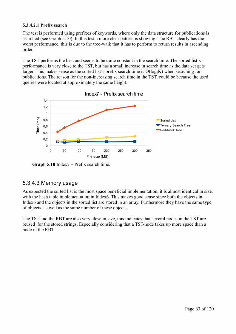
5.3.4.2.1 Prefix searchThe test is performed using prefixes of keywords, where only the data structure for publications is searched (see Graph 5.10). In this test a more clear pattern is showing. The RBT clearly has the worst performance, this is due to the tree-walk that it has to perform to return results in ascending order.

The TST performs the best and seems to be quite constant in the search time. The sorted list´s performance is very close to the TST, but has a small increase in search time as the data set gets larger. This makes sense as the sorted list´s prefix search time is O(log2K) when searching for publications. The reason for the non-increasing search time in the TST, could be because the used queries were located at approximately the same height.

5.3.4.3 Memory usageAs expected the sorted list is the most space beneficial implementation, it is almost identical in size, with the hash table implementation in Index6. This makes good sense since both the objects in Index6 and the objects in the sorted list are stored in an array. Furthermore they have the same type of objects, as well as the same number of these objects.

The TST and the RBT are also very close in size, this indicates that several nodes in the TST are reused for the stored strings. Especially considering that a TST-node takes up more space than a node in the RBT.

of 120

Graph 5.10 Index7 – Prefix search time.

0 50 100 150 200 250 300 3500

0,2

0,4

0,6

0,8

1

1,2

1,4

Index7 - Prefix search time

Sorted ListTernary Search TreeRed-black Tree

File size (MB)

Tim

e (m

s)

5.3.5 ConclusionThe prefix search functionality was implemented using the three data structures the sorted list, the TST, and the RBT. It was initially stated that the most efficient data structure would be chosen since one of the main criteria of the project is to develop a high performance search engine. Furthermore looking besides performance the TST and the RBT have the advantage of being dynamic, that is elements can be added and deleted. Given the way data is parsed into the data structure in this project, performance will be rated higher than the dynamic feature.

The full search test was approximately equal for all three implementation and will therefore not influence which data structure that is chosen.

The RBT is the first implementation to not be considered further, as its prefix search time is too slow compared to the two others. Furthermore the RBT is not the most space efficient either.

The choice is therefore between the sorted list and the TST; the sorted list was clearly the most space efficient implementation, whereas the TST has a slightly faster prefix search time. Since the difference in prefix search time is so small, the sorted list will be used in the following updates.

of 120


0 50 100 150 200 250 300 3500

200

400

600

800

1000

1200

1400

Index 7 - Memory usage

Sorted ListTernary Search TreeRed-black TreeIndex6

File size (MB)

Mem

ory

(MB

)

5.4 Index8 – Integer ArrayIn this update the focus will be on improving the program´s space usage, this is done by using Integer arrays. That is storing lists of integers instead of list of objects, where each integer maps to the object it is representing.

In the previous versions of the search engine, each keyword and name object contained linked lists of authors and publications (See Figure 5.5). This implementation uses a lot of space, for the following reasons:

• PointersEach object in the linked lists has an object reference to the next object in the list. More formally, each publication object has two pointers; a pointer to the next publication object in the linked list and a pointer to the start of its linked list of authors. Likewise the author object has a pointer to the next author and a pointer to the start of its list of publications. Furthermore each keyword object has a pointer to its linked list of publications and each name object a pointer to its linked list of authors.

• Multiple objects In order to build the linked lists, an object must be created for each element in the list. Therefore since e.g. a publication can have several authors, the publication is stored as an object in each of its authors linked lists. The same multiple object creation, also happens in both the keyword, name and the author object´s linked lists as well. Even though all the objects representing e.g. a publication point to the same title string, it still uses a lot of space to create all these objects.

To improve the space usage, these cases are handled by the introduction of the integer array. The following changes are made to the data structure:

• Two new lists are added to store the author and publication objects, one for each type. Objects are added to the lists in the order they are parsed from the data set.

• All linked lists have been replaced with lists that store integers. Each integer works as an ID for the object, for example a keyword´s list of publication IDs, all maps to the publication objects, that is a publication ID is the publication´s position in the list of publication objects. Similarly author IDs are the author object´s positions in the list of author objects.

The data structure for Index8 is shown in Figure 5.8.

of 120

5.4.1 InitializationThe algorithms for parsing the data in to the data structure have been modified in this update, but still most of the running time analysis remain the same. Therefore several parts of the analysis remains the same as in the analysis of the sorted list in Index7 (Section 5.3.1.1). Therefore these part´s running times are only summarized and not explained in detail.

The following list is for every time a publication or an author is parsed from the file.1. Iterating through all the words in a title / name

O(1)

2. Testing if word is a keyword / namepartO(1)

of 120

Figure 5.8 The data structure of Index8. The data structure consists of the two sorted lists names and keywords. Furthermore there are two lists storing the objects; authors stores the author objects and publications stores the publication objects. Each keyword object has a list of integers, that is the publication IDs. Each name object also has a list of integers, that is the author IDs. The dotted grey lines show the mapping from author or publication IDs, to the lists containing the author and publication objects (mappings are for simplicity, not shown for all the IDs in the lists. In practice there would be no empty positions between the stored integers.)

DynamicArray<String namePart , Name n> names

N1

DynamicArray<Integer> authorIDs

DynamicArray<Author> authors

DynamicArray<Integer> publicationIDs

A1

DynamicArray<String keyword, Keyword k> keywords

K1

DynamicArray<Integer> publicationIDs

DynamicArray<Publication> publications

DynamicArray<Integer> authorIDs

P1

3. Searching the sorted lists for duplicate keywords / namepartsThe running time for searching the sorted list of keywords O(log2 K) The running time for searching the sorted list of nameparts O(log2 N)

4. Inserting keyword / namepart .Inserting into the list of keywords O(K)Inserting into the list of nameparts O(N)

5. Inserting the publication in the keyword´s list / inserting the author in the namepart´s listInserting into these lists requires a duplication check, especially since the same authors can appear many times in the data file, furthermore there can be special cases where duplicate publication titles occur and since this update is dependent on unique author and publication IDs, the check is there to ensure this property.

When searching for duplicate author or publication objects, a natural solution would be to iterate through the corresponding list of objects e.g. authors (see Figure 5.8). This solution though would increase the initialization time substantially, as it would take O(P) and O(A) time to search these lists. Instead the following deduction is used in the algorithm; if e.g. a publication is already in the list, then the publication´s keywords must be added to the sorted list keywords. Therefore iff the keyword is not in the sorted list, the publication cannot be in the list of publications either. Since the same keyword could have been added for another publication, the keyword´s list must be searched as well. The same deduction is used for authors and their nameparts.

Therefore a binary search is performed on the sorted list of either keywords or nameparts, which was already done in step3 and the object´s position is therefore already known. So to check for duplicate publications or authors, the object´s list must be searched. This takes the linear running time corresponding to the size of the list.

Searching for duplicates and inserting the publication in the keyword´s list O(p)Searching for duplicates and inserting the author in the nameparts´s list O(a)

The following procedure is initiated after the above list is completed.

Inserting author IDs into the publication´s list / Inserting the publication ID into the authors listsIn the previous section this was possible in constant time, as e.g. the authors could be stored directly on the fly into the created publication object, before starting the procedures in above list. Now this is not possible, since it is the IDs that is added and not the objects. And the ID of an object is not known before the procedures in the above list are completed, this is because of the way the algorithm searches for duplicate author and publication objects.

The author and publication object´s lists must be searched for duplicate IDs, so the running time depends on the number of elements in a list. There clearly is a limit to how many authors there have been a part of a publication, therefore the publication´s list of authors will be seen as a constant. The author´s list of publications on the other hand, is quite larger, for instance Edsger Dijkstra has 65 publications listed in the data file. This factor will be described with the variable “u”.

of 120

Step5 in the analysis list and the added procedure after the completion of this list, are the only parts that have changed compared to the sorted list in Index7.

The total running time for the initialization can then be expressed by O(P(log2(K) + K + p) + A(log2(N) + N + a) + u). The initialization is still expected to have a quadratic behaviour, but due to the extra variable u, the initialization time should be slower than in the sorted list in Index7 (see Graph 5.12)

5.4.2 SearchingThe only change made to the search algorithms, is that now a list of integers is returned, instead of a reference to a linked list of objects. To output the result, the objects must now be retrieved from object lists, by using the integers. This only requires one operation per object, as the integer is the object´s position. Therefore there is no change in the analysed search time, compared to the sorted list in Index7 (Section 5.3.1.2).

The total time for a full search is O(log2(K) + p) when searching for publications and O(log2(N) + a) when searching for authors.

The total prefix search time is O(log2K) when searching for publications and O(log2N) when searching for authors.

5.4.3 Space usageIn this implementation all the object references used by the linked lists have been removed, by switching to arrays. And instead of creating multiple objects, integers are used to represent the objects´ positions. This way only one object for each unique publication or author is created. In Java an object reference uses 8 bytes, where an integer only uses 4 bytes of memory. Therefore a reduction in space usage is expected. (Graph 5.14).


5.4.4.1 Initialization timeThe measured initialization time still follows a quadratic function, as expected the time is now slower than the sorted list in Index7. This fits well with the analysed running time, where the only difference is the added variable u in Index8.

of 120

Graph 5.12 Index8 – Initialization time comparison to Index7.The calculated functions: Index8: y = 0,0191x2 – 1,7613x and Index7: y = 0,0071x2 + 0,1176x.

0 50 100 150 200 250 300 3500

200

400

600

800

1000

1200

Initialization time

Index8 – Integer ArrayIndex7 – Sorted list

File size (MB)

Tim

e (s

)

5.4.4.2 Memory usageGraph 5.13 shows that the memory usage is still linear with the size of the input file, furthermore with this implementation it is now possible to load in the complete DBLP file of 750MB.

The measured memory usage for Index7 and Index8 are very close for the smaller files, for the 25MB and 50MB files Index7 actually performs a bit better. This should not be the case, but potentially it could be because of the way Java allocates memory. Java sometimes allocate more memory than the program needs (see Section 2.4.1). As the files gets bigger Index8 clearly outperforms Index7. The graphs´ calculated functions shows that Index7´s gradient is ((3,5478/2,9522) - 1 = 0,20) 20% bigger, thus this update has improved the memory usage with approximately (1-(2,9522/3,5478) = 0,17) 17%. Furthermore by using the computed function, Index7´s memory usage for the 750MB file can be calculated: 3,5478 ∙750 = 2661MB. Now the reduction in used memory can be estimated for the biggest data file: 2661MB - 2214MB = 447MB. That is, Index8 uses roughly 450MB less memory than Index7 for the 750MB file.

of 120


0 100 200 300 400 500 600 700 8000

500

1000

1500

2000

2500


Integer Array

File size (MB)

Mem

ory

(MB

)

Graph 5.14 Index8 – Memory usage comparison to Index7.The calculated functions for the graphs are; Index8: y = 2,9522x and Index7: y = 3,5478x.

0 50 100 150 200 250 300 3500

200

400

600

800

1000

1200

Memory usage

Index8 – Integer ArrayIndex7 – Sorted list

File size (MB)

Mem

ory

(MB

)

5.5 Index9 – Boolean SearchIn the previous versions of the search engine, it was only possible to search for one word at a time, either by using a namepart or a keyword. The problem with this can be, that for some queries e.g. a common last name, there is a lot of results, which makes it tedious for the user to find what he/she is looking for. The boolean search makes it possible to do queries using several words. The boolean search is a search method that finds the intersection between two lists (see section 3.7).

This update just provides additional search functionalities and therefore does not affect the initialization time or the general space usage, therefore these will not be analysed or measured.

5.5.1 The boolean search algorithmThe algorithm takes two lists as input and returns the intersection of these.

This could be achieved by a brute force approach, where each item from the first list is compared with each item from the second list. This approach will results in the search time O(L1 * L2), where L1 and L2 are the size of the two lists accordingly.

A faster approach is possible if the input lists are in sorted order. In the following description the assumption is made that the input lists are sorted in ascending order. The algorithm works by comparing the first item from each list (the items with the lowest “value” from each list) and iterates through the lists depending on comparisons. At each comparison there are three possibilities

1. The items are equal; one of the items is added to the intersection list and the algorithm moves one position forward in each list.

2. The item from the first list is smaller that the item from the second list; the algorithm moves one position forward in the first list.

3. The item from the second list is smaller that the item from the first list; the algorithm moves one position forward in the second list.

The performance of this algorithm is O(L1 + L2). This is the case since on any outcome of a comparison, the algorithm can move at least one position forward in one of the lists. That is, it “removes” the smallest item or both items if they are equal, after each comparison.

5.5.2 Applying the boolean searchAll authors and publications in the application are represented by an integer (ID) as described in Index8. As the objects´ IDs are generated in an incremental fashion, as they are parsed from the file, these IDs in some cases conveniently get stored in ascending order. These cases are

• Keyword´s list of publication IDs

• Namepart´s list of author IDs.

• Author´s list of publication IDs

A publication´s list of author IDs, is not in sorted order, since authors are listed for each publication they have been a part of. So an author might be added first for one publication and as the last for an other.

of 120

The boolean search can also be used to find the intersection between a variable number of lists. This is done by finding the intersection between the first two lists and then the intersection between the result of the first intersection and the third list, this procedure continues until all lists are intersected (see Figure 5.9).

Figure 5.9 The procedure for finding the intersection between n lists. The variables L denotes the lists and R denotes the result of an intersection.

The worst case running time for intersecting n lists is the lengths of all the lists and the time it takes to loop through the n lists. The number of lists correspond to the number of words in the query, therefore looping through the lists is seen as a constant. The running time can be expressed by O(L1

+ L2 + … + Ln). In most cases the result list R will get less elements as more intersections are performed.

With this information in mind the search functionalities will now be described. In this application the boolean search will be implemented to support three search functionalities:

1. Searching for publications using multiple keywordsWith this functionality it is easier to find specific publications, as it makes it possible to search for several keywords in the title. The search procedure works by querying the sorted list of keywords, for each keyword in the search string, each query returns a list of publication IDs in sorted order. The lists are then parsed to the boolean search algorithm according to Figure 5.9.

2. Searching for authors using multiple namepartsThis search functionality makes it possible to search for more than one namepart at a time e.g. the user can search for both the first and the last name of an author and thus narrow down the results substantially. The search procedure works by querying the sorted list of names, for each word in the search string, each query returns a list of author IDs in sorted order. The lists are then parsed to the boolean search algorithm according to Figure 5.9.

3. To find all the publications co-authored by the specified authors. A boolean search for the two authors A and B would return a list of publications corresponding to the intersection between author A´s list of publications and author B´s list of publications. To perform this search, the specific author objects are needed to return the correct result, therefore author IDs are used as input. This is necessary since it is only possible to find authors by searching for nameparts, a query for a first and last name might return more than one result, hence a boolean search might not return the publications the user was looking for. The idea is, that the user uses the search functionality (2) described above as a retrieval system for the author ID.

5.5.3 Search timeTo perform a boolean search in the application, just type the queries separated by a white space. The search type is specified through the console based menu. Therefore parsing the string into separate words will be seen as a constant.

In the following analysis the variable W is the number of words in the search string.

of 120

R=L1∩L2⇒ R=R∩L3⇒ ....⇒ R=R∩Ln

5.5.3.1 Searching for publications using multiple keywordsA query on the sorted list of keywords is performed for every word in the search string, each query returns a sorted list of publication IDs, the variable p describes the length of these lists. Searching the sorted list W times takes O(W ∙ log2(K)) time. Since there are W lists of size p, finding the intersection takes O(W ∙ p) time. The total search time is therefore O(W ∙ (log2(K) + p)).

5.5.3.2 Searching for authors using multiple namepartsA query on the sorted list of nameparts is performed for every word in the search string, each query returns a sorted list of author IDs, the variable a describes the length of these lists. Searching the sorted list W times takes O(W ∙ log2(N)) time. Since there are W lists of size a, finding the intersection takes O(W ∙ a) time. The total search time is therefore O(W ∙ (log2(N) + a)).

5.5.3.2 Searching for publications co-authored by the specified authorsFor each author ID in the search string, the author object´s list of publication IDs is retrieved, the variable u describes the length of these lists. Retrieving W author objects takes O(W) time and since there are W lists of the size u, finding the intersection takes O(W ∙ u) time. The total search time is therefore O(W ∙ u).

5.5.4 Performance test and analysisThe test shows that the boolean search has a linear growth with the file size. This makes sense as the used keywords are very common in the titles and therefore the lists for the keywords grow bigger as more publications are added to the data structure.

of 120

Graph 5.15 Index9 – Boolean search time. The test was performed searching for publications, using the queries “algorithm” and “fast”.

0 50 100 150 200 250 300 3500

0,2

0,4

0,6

0,8

1

1,2

1,4

Index9 - Boolean search time

Boolean search

File size (MB)

Tim

e (m

s)

5.6 Index10 – Web ApplicationThis update will consist of two parts

1. Extending the program into a web application.

2. The implementation of the web based GUI, that supports the ordinary full search, the auto-suggest feature described in Index7, and the boolean searches described in Index9.

5.6.1 The web applicationOverall the web application works by using web pages to display the content and a servlet to process the requests from the client, that is when a user makes a query from the web page the servlet will process the query and return the result to the client.

On the client side requests to the servlet are done in two ways, either by filling an input field and submitting the form by clicking the button or dynamically while the user types with the use of AJAX6. How the requests are handled is further elaborated in the descriptions for the individual parts of the GUI.

In the previous versions, the data file was loaded into the data structure when the program was started, this is done a bit different as the web application must be run on a server. Therefore to get the data loaded into the data structure, this procedure is called from the servlet´s init method, and in the project´s configuration file web.xml the servlet is set to load on start up. This way the data is made available for querying before the web application is launched.

5.6.2 The web based GUIThe main page of the GUI can be inspected in Figure 5.9, it consists of three main parts:

• The search field – This is the input field where the user can type the desired query. This field is both used for the full search feature and the boolean search on names and titles. Furthermore a list of suggestions will appear, if the current string in the search field is a prefix of a namepart or a keyword. (see Figure 5.11)

• Selection menu – In this menu the user chose whether to search for authors or publications. (see Figure 5.10)

• Dynamic iframe – The idea of the iframe is that the user gets a feeling of never leaving the main page, all pages are dynamically loaded in the iframe; whether it is the result of a full search (Figure 5.12), a boolean search (Figure 5.13, 5.14, and 5.15) or the information of a found publication or author (Figure 5.16).

The last boolean search, that is the search for publications co-authored by two specific authors is performed on a separate web page. This page is loaded as the default page in the iframe or it can be accessed by clicking the link below the iframe-box. (see Figure 5.9 and 5.15).

6 Asynchronous JavaScript and XML

of 120

5.6.2.1 The selection menuThe chosen type in the selection menu specifies whether to search for authors or publications, If option “author” is chosen, then the sorted list containing nameparts is searched and when the option “publication” is chosen the sorted list of keywords is searched. This information is send to theservlet when a query is made, by setting the chosen type in the URL e.g. type=author. This should narrow down the search results and thus make it easier for the user to find he/she is looking for.

5.6.2.1 Auto-suggest menuThe auto-suggest menu is the list of results that appears below the search field while the user is typing. This search functionality is implemented using AJAX, which is initiated when an onkeyup event occurs in the search field, that is for every time time a key is pressed.

of 120

Figure 5.10 The selection menu. The menu is used for specifying whether to search for authors or publications.

Figure 5.9 The front page of the search engine. The Boolean search page is loaded as the default in the iframe.

The following list describes the process of the AJAX interaction with the servlet:

1. When the onkeyup event occurs the AJAX function is initiated.

2. The XMLHttpRequest object is created according to the browser type.

3. The XMLHttpRequest object makes a call to the servlet using a HTTP GET request. This is done by concatenating the current string in the search field and the chosen type in the selection menu to the URL e.g. search?action=auto&q=dij&type=author. The action parameter tells the servlet that the query is a prefix search.

4. The servlet processes the request; more formally it performs a prefix search on the sorted list according to the chosen type in the selection menu.

5. The servlet returns the result. The result is generated as text instead of XML, the reason is that the content of the result is quite simple and it is therefore easier to process at both the client and the server side.

6. The XMLHttpRequest calls the handleServerResponse function and processes the result. That is it waits for the server to call it with the ready state 4, which signifies that the response is completed. Furthermore a check is performed if the HTTP interaction was successful. Now the data returned by server can be used to update the auto-suggest menu, this is done by calling the function updatePage.

7. When the updatePage function is called the HTML DOM is updated. The auto-suggest menu is made as an unordered list, where each author or publication in the response text is appended as a list item. Each list item is a generated link to an author´s or publication´s information page (Figure 5.16), where the text shown is either the name of an author or the title of a publication.

The auto-suggest menu is shown in Figure 5.11.

5.6.2.2 Full searchThe full search is performed by typing the desired words in search field and pressing the search button. When the button is clicked a script is called to set the URL in the iframe and thus the servlet is invoked within the iframe. The URL contains all the parameters the servlet needs to perform the full search procedure; action is set to full, type is set according to the chosen type in the selection menu, and query is set to the string in the search field e.g. search?action=full&type=publication&query=algorithm. (see Figure 5.12).

of 120

Figure 5.11 The auto-suggest menu searching for authors.

5.6.2.3 Boolean searchThe two boolean search functionalities; searching for authors using nameparts (see Figure 5.14) and searching for publications using keywords (see Figure 5.13) are performed similarly to the full search. The query is typed in the search field, words are separated with a white space, and the URL is loaded in the iframe. The URL is basically the same as in the full search, now the parameter query is just set to hold all the words e.g. search?action=full&query=fast algorithm&type=publication.

of 120

Figure 5.13 Boolean search – searching for publications using the keywords “fast” and “algorithm”.

Figure 5.12 Full search – searching for publications using the keyword “algorithm”.

The 3rd boolean search functionality described in section 5.5.2, where all publications which is co-authored by two chosen authors is returned, is handled a bit different. This search functionality has its own web page consisting of two forms (see Figure 5.9), one to find the IDs´ for the authors and a second to make the actual search for publications using the found authorIDs´ The idea is that the search for authors should work as a retrieval system to get the ID´s.

of 120

Figure 5.14 Boolean search – searching for authors using the nameparts “john” and “backus”.

Figure 5.15 Boolean search – searching for publications co-authored by Stephan Olario and Rong Lin, using their authorIDs´ 5759 and 21230.

5.6.2.4 LookupLookup is the functionality that retrieves an author´s or a publication´s information and is used whenever an author or publication link is clicked. This makes it possible to navigate between the search results and the information pages. The lookup method works by generating dynamics links, the action parameter is set to lookup, type is set according to what is chosen in the selection menu, and the ID is the object´s position in either the list of publication objects or the list of author objects. For example the url search?action=lookup&id=14216&type=author generates the page for the author “Edsger W. Dijkstra” with used data file. (see Figure 5.16)

The lookup procedure is done in O(1) time as the ID maps directly to the object´s position.

of 120

Figure 5.16 Lookup – Showing the generated information in the iframe, for the author Edsger W. Dijkstra.

6 Functional TestsScreen shots of the test results can be found in the appendix (Section 10.1.2).

6.1 Index1

Table 6.1 Index1 - Functional test. (Screen shot in Figure 10.1)

Test case Query Expected result Actual result StatusSearching for an author who exists in the file.

Craig Larman Craig Larman exists Craig Larman exists PASS

Searching for an author who exists in the file.

Edsger W. Dijkstra

Edsger W. Dijkstra exists

Edsger W. Dijkstra exists PASS

Searching for an author who is not the file.

X X does not exist X does not exist PASS

6.2 Index2


Test case Query Expected result Actual result StatusSearching for an author who is one of several co-authors of a publication.

Joseph Henry Wegstein

Revised report on the algorithm language ALGOL 60.Joseph Henry Wegstein exist

Revised report on the algorithm language ALGOL 60.Joseph Henry Wegstein exist

PASS

Searching for an author with several publications.

Edsger W. Dijkstra

Letters to the editor: go to statement considered harmful.Algorithms 3Algorithms 2Algorithms 1Edsger W. Dijkstra exist

Letters to the editor: go to statement considered harmful.Algorithms 3Algorithms 2Algorithms 1Edsger W. Dijkstra exist

PASS

Searching for an author who is not the file.

X X does not exist X does not exist PASS

of 120

6.3 Index3


Test case Query Expected result Actual result StatusSearch for an author who is the only author of a publication.

Craig Larman APPLYING UML AND PATTERNS

APPLYING UML AND PATTERNS

PASS

Search for authors who is co-authors of a publication.

1) John W. Backus

2) Peter Naur

Revised report on the algorithm language ALGOL 60.


PASS

Search for non-existent author.

XXX The author was not found.

The author was not found. PASS

Searching for an author who is author of several publications.

Edsger W. Dijkstra

Algorithms 2Letters to the editor: go to statement considered harmful.


PASS

Test size of the linked list of authors.

N/A 15 15 PASS

of 120

6.4 Index4

Table 6.4 Index4 - Functional test. Hash table size is set to 3 to make testing for collisions easier. (Screen shot in Figure 10.4)

Test case Query Expected result Actual result StatusTest number of inserted authors.

N/A 15 (The unique number of authors)

15 PASS

Test number of inserted publications.

N/A 17 (The publication must be inserted for each author)

17 PASS

Search for an author who is the only author of a publication.



PASS


1) John W. Backus

2) Peter Naur



PASS

Search for non-existent author.

xxx The author was not found.

The author was not found. PASS


1) Edsger W. Dijkstra

2) Julien Green

1) Algorithms 2Letters to the editor: go to statement considered harmful.2)Algorithms 2Revised report on the algorithm language ALGOL 60.

1) Algorithms 2Letters to the editor: go to statement considered harmful.2)Algorithms 2Revised report on the algorithm language ALGOL 60.

PASS

of 120

6.5 Index5

Table 6.5 Index5 - Functional test. Hash table size is set to 3 to make testing for collisions easier. (Screen shot in Figure 10.5)

Test case Query Expected result Actual result StatusSearch for a publication with one author


Craig Larman Craig Larman PASS

Search for a publication with several co-authors


Peter NaurMichael WoodgerAdriaan van WijngaardenJoseph Henry WegsteinBernard VauquoisKlaus SamelsonHeinz RutishauserAlan J. PerlisJohn L. McCarthyC. KatzJulien GreenFriedrich L. BauerJohn W. Backus

Peter NaurMichael WoodgerAdriaan van WijngaardenJoseph Henry WegsteinBernard VauquoisKlaus SamelsonHeinz RutishauserAlan J. PerlisJohn L. McCarthyC. KatzJulien GreenFriedrich L. BauerJohn W. Backus

PASS

Search for a non existing author or publication

X No matches found. No matches found. PASS

Search for an author who is the only author of a publication.



PASS


1) John W. Backus

2) Peter Naur



PASS


Edsger W. Dijkstra



PASS

of 120

6.6 Index6


Test case Query Expected result Actual result StatusSearch for a keyword with several publications

algorithms Keyword was found, printing publications and the authors

Algorithms 1Julien Green1Edsger W. Dijkstra



Keyword was found, printing publications and the authors




PASS

Search for a keyword with one publication

patterns Keyword was found, printing publications and the authors

APPLYING UML AND PATTERNSCraig Larman

Keyword was found, printing publications and the authors

APPLYING UML AND PATTERNSCraig Larman

PASS

Search for a namepart with several authors

Julien Name was found, printing authors and their publications

Julien Green1Algorithms 1



Julien GreenRevised report on the algorithm language ALGOL 60.

Name was found, printing authors and their publications




Julien GreenRevised report on the algorithm language ALGOL 60.

PASS

of 120

Table 6.7 Index6 - Functional test part2. (Screen shot in Figure 10.7)

Test case Query Expected result Actual result StatusSearch for a namepart with one author

Dijkstra Name was found, printing authors and their publications

Edsger W. DijkstraAlgorithms 1Algorithms 2Algorithms 3Letters to the editor: go to statement considered harmful.

Name was found, printing authors and their publications

Edsger W. DijkstraAlgorithms 1Algorithms 2Algorithms 3Letters to the editor: go to statement considered harmful.

PASS

Search for a word in a title, which does not qualify to be a keyword.

the No match was not found.

No match was not found.

PASS

Search for a word in a name, which does not qualify to be a namepart.

W. No match was not found.

No match was not found.

PASS

of 120

6.7 Index7The inner data structure has already been tested, therefore only tests on the outer data structure is performed.

Table 6.8 Index7 – Prefix search - Functional test. (Screen shot in Figure 10.8 and 10.9)The same test was performed on all three data structures, with the same result.

Test case Query Expected result Actual result StatusSearch using the prefix of a namepart

d Prefix mached a name, printing author namesEdsger W. Dijkstra

Prefix mached a name, printing author namesEdsger W. Dijkstra

PASS

Search using the prefix of a keyword

alg Prefix matched a keyword in a title, printing publication and its authorsRevised report on the algorithm language ALGOL 60.Revised report on the algorithm language ALGOL 60.Algorithms 1Algorithms 2Algorithms 3

Prefix matched a keyword in a title, printing publication and its authorsRevised report on the algorithm language ALGOL 60.Revised report on the algorithm language ALGOL 60.Algorithms 1Algorithms 2Algorithms 3

PASS

The full search on a namepart

Julien no publications found

Full searh mached a name, printing authors.Julien Green1Julien Green2Julien Green3Julien Green

no publications found

Full searh mached a name, printing authors.Julien Green1Julien Green2Julien Green3Julien Green

PASS

The full search on a keyword

Algorithms no authors found

Full search matched a keyword in a title, printing publication.Algorithms 1Algorithms 2Algorithms 3

no authors found

Full search matched a keyword in a title, printing publication.Algorithms 1Algorithms 2Algorithms 3

PASS

of 120

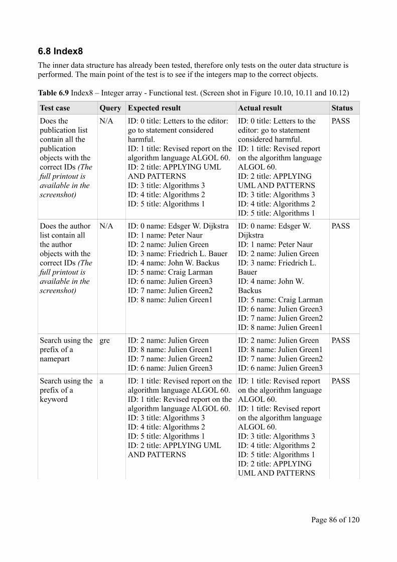
6.8 Index8The inner data structure has already been tested, therefore only tests on the outer data structure is performed. The main point of the test is to see if the integers map to the correct objects.

Table 6.9 Index8 – Integer array - Functional test. (Screen shot in Figure 10.10, 10.11 and 10.12)

Test case Query Expected result Actual result StatusDoes the publication list contain all the publication objects with the correct IDs (The full printout is available in the screenshot)

N/A ID: 0 title: Letters to the editor: go to statement considered harmful.ID: 1 title: Revised report on the algorithm language ALGOL 60.ID: 2 title: APPLYING UML AND PATTERNSID: 3 title: Algorithms 3ID: 4 title: Algorithms 2ID: 5 title: Algorithms 1

ID: 0 title: Letters to the editor: go to statement considered harmful.ID: 1 title: Revised report on the algorithm language ALGOL 60.ID: 2 title: APPLYING UML AND PATTERNSID: 3 title: Algorithms 3ID: 4 title: Algorithms 2ID: 5 title: Algorithms 1

PASS

Does the author list contain all the author objects with the correct IDs (The full printout is available in the screenshot)

N/A ID: 0 name: Edsger W. DijkstraID: 1 name: Peter NaurID: 2 name: Julien GreenID: 3 name: Friedrich L. BauerID: 4 name: John W. BackusID: 5 name: Craig LarmanID: 6 name: Julien Green3ID: 7 name: Julien Green2ID: 8 name: Julien Green1

ID: 0 name: Edsger W. DijkstraID: 1 name: Peter NaurID: 2 name: Julien GreenID: 3 name: Friedrich L. BauerID: 4 name: John W. BackusID: 5 name: Craig LarmanID: 6 name: Julien Green3ID: 7 name: Julien Green2ID: 8 name: Julien Green1

PASS

Search using the prefix of a namepart

gre ID: 2 name: Julien GreenID: 8 name: Julien Green1ID: 7 name: Julien Green2ID: 6 name: Julien Green3

ID: 2 name: Julien GreenID: 8 name: Julien Green1ID: 7 name: Julien Green2ID: 6 name: Julien Green3

PASS

Search using the prefix of a keyword

a ID: 1 title: Revised report on the algorithm language ALGOL 60.ID: 1 title: Revised report on the algorithm language ALGOL 60.ID: 3 title: Algorithms 3ID: 4 title: Algorithms 2ID: 5 title: Algorithms 1ID: 2 title: APPLYING UML AND PATTERNS

ID: 1 title: Revised report on the algorithm language ALGOL 60.ID: 1 title: Revised report on the algorithm language ALGOL 60.ID: 3 title: Algorithms 3ID: 4 title: Algorithms 2ID: 5 title: Algorithms 1ID: 2 title: APPLYING UML AND PATTERNS

PASS

of 120

6.9 Index9

Table 6.9 Index8 – Boolean search - Functional test. (Screen shot in Figure 10.13, 10.14 and 10.15)

Test case Query Expected result Actual result StatusSearching for a publication using two keywords

algorithm ALGOL

ID: 1 title: Revised report on the algorithm language ALGOL 60.ID: 2 title: algorithm language ALGOL 60.ID: 5 title: algorithm ALGOL 60.ID: 6 title: The fast algorithm language ALGOL 99.

ID: 1 title: Revised report on the algorithm language ALGOL 60.ID: 2 title: algorithm language ALGOL 60.ID: 5 title: algorithm ALGOL 60.ID: 6 title: The fast algorithm language ALGOL 99.

PASS

Searching for a publication using three keywords

algorithm ALGOL fast

ID: 6 title: The fast algorithm language ALGOL 99.

ID: 6 title: The fast algorithm language ALGOL 99.

PASS

Searching for an author using two nameparts

Peter Naur ID: 1 name: Peter Naur ID: 1 name: Peter Naur PASS

Searching for an author using three nameparts

Peter Ben Nielsen

ID: 14 name: Peter Ben Nielsen

ID: 14 name: Peter Ben Nielsen

PASS

Search for publications co-authored by two specified authorIDs

1 13 ID: 1 title: Revised report on the algorithm language ALGOL 60.

ID: 1 title: Revised report on the algorithm language ALGOL 60.

PASS

of 120

6.10 Index10Table 6.11 Index10 – Web application - Functional test. (Screen shot in Figure 10.16, 10.17, 10.18, 10.19, and 10.20)Test case Query Expected result Actual result StatusIf the auto-suggest menu works for authors

g Julien GreenJulien Green1Julien Green2Julien Green3

Julien GreenJulien Green1Julien Green2Julien Green3

PASS

If the auto-suggest menu works for publications

algor Revised report on the algorithm language ALGOL 60.Algorithms 1Algorithms 2Algorithms 3

Revised report on the algorithm language ALGOL 60.Algorithms 1Algorithms 2Algorithms 3

PASS

If generated links work e.g. in auto-suggest menu and in search results.

N/A Opens page for selected item

Opens page for selected item

PASS

Boolean search in search field

algorithm language



PASS

Boolean search with author IDs

1 3 Revised report on the algorithm language ALGOL 60.


PASS

of 120

7 Future improvementsThere is still several improvements that could be implemented in the search engine, following is a brief description of extensions that could improve the search engine.

7.1 Spell checkThe spell check should suggest alternative results that almost match the query, especially in the case where no results is found, furthermore it could be integrated into the auto-suggest functionality.

7.2 Elias Gamma CodingThis extension would help reduce the space usage even further.

7.3 Extra search functionalitiesThe extra search functionalities should make it easier for the user to narrow down the search results. For example being able to search within given dates of time or being able to perform property specific searches.

of 120

8 ConclusionThe overall goal of the project was to develop a scalable and high performance search engine, based on the publication database ”The DBLP Computer Science Bibliography”. Where the highest priority in the the advanced part was finding and evaluating data structures which efficiently supports the search functionality auto-suggest7 and implementing the solution in a web application.

The effort done throughout the last three months has resulted in a search engine that supports the auto-suggest functionality, where the shown suggestions are based on prefix searches on single words in names and titles. Three data structures supporting the prefix search was implemented and tested, the sorted list was chosen due to its low space usage and its highly competitive search time; only the ternary search tree performed slightly better on the prefix searches. Furthermore it is also possible to perform ordinary searches using one or more words in the query. The memory usage was reduced by the implementation of a stop word filter and integer arrays. These memory reducing techniques made it possible to load the complete 750 MB data file into the data structure.

The search engine could with some minor tweaks be implemented to work on other types of data files as well or combined with a web crawler. A thing to consider if extending the search engine to support other types of data files, is the implemented filter. The stop word filter proved very efficient in this project without worsening the search results, this was due to the fact that all stop words was hand picked for the DBLP8 data set. However for other types of data the current filter might not work as well e.g. it would not be possible to find the movie “IT” or the band “The Who”, as all these words are currently removed. Therefore an analysis of the used data would be recommended before using a stop word filter. Fortunately once the data has been analysed it is very easy to implement the filter.

The incremental development process proved very useful in this project, when basically implementing the search engine from scratch, as it helped keeping perspective on all the considered requirements. Furthermore it helped breaking down a complex task into more comprehensible sub problems and to keep overview of the time by using a time plan for the increments.

With all things considered, I am very satisfied with the result and believe that the overall goal of the project has been met.

7 Search functionality which dynamically provides suggestions while the user is typing.8 Digital Library and Bibliography Project.

of 120

9 ReferencesBook references:

[B1] Title: Introduction to Algorithms, Second Edition.Authors: Thomas H. Cormen, Charles E. Leiserson, Ronald L. Rivest, and Clifford Stein.

[B2] Title: Algorithms in Java, 3rd Ed, Part 4.Author: Robert Sedgewick.

Internet References:

[I1] Search Engine Project – Project Descriptionhttp://searchengineproject.wordpress.com/

[I2] The DBLP Computer Science Bibliographyhttp://www.informatik.uni-trier.de/~ley/db/

[I3] Video tutorial: NetBeans IDE 6 Profilerhttp://medianetwork.oracle.com/media/show/14757?n=playlist&nid=81

[I4] Short article about stop wordshttp://en.wikipedia.org/wiki/Stop_words

[I5] List of common English stop wordshttp://www.textfixer.com/resources/common-english-words.txt

[I6] Pizza&chili Corpushttp://pizzachili.di.unipi.it/index.html

[I7]Porter Stemming Algorithmhttp://tartarus.org/~martin/PorterStemmer/

[I8] Inverted Indexhttp://en.wikipedia.org/wiki/Inverted_index

[I9] Ternary Search Trees by Jon Bentley and Bob Segdewickhttp://www.drdobbs.com/windows/184410528

[I10] Plant your data in a ternary search tree by Wally Flint.http://www.javaworld.com/javaworld/jw-02-2001/jw-0216-ternary.html

[I11] Mastering AJAX, Part 1: Introduction to Ajaxhttp://www.ibm.com/developerworks/web/library/wa-ajaxintro1.html

[I12] Mastering AJAX, Part 2: Make asynchronous requests with JavaScript and Ajaxhttp://www.ibm.com/developerworks/web/library/wa-ajaxintro2/

of 120

http://www.ibm.com/developerworks/web/library/wa-ajaxintro2/

http://www.ibm.com/developerworks/web/library/wa-ajaxintro1.html

http://www.javaworld.com/javaworld/jw-02-2001/jw-0216-ternary.html

http://www.drdobbs.com/windows/184410528

http://en.wikipedia.org/wiki/Inverted_index

http://tartarus.org/~martin/PorterStemmer/

http://pizzachili.di.unipi.it/index.html

http://www.textfixer.com/resources/common-english-words.txt

http://en.wikipedia.org/wiki/Stop_words

http://medianetwork.oracle.com/media/show/14757?n=playlist&nid=81

http://www.informatik.uni-trier.de/~ley/db/

http://searchengineproject.wordpress.com/

[I13] Mastering Ajax, Part 3: Advanced requests and responses in Ajaxhttp://www.ibm.com/developerworks/web/library/wa-ajaxintro3/

[I14] Mastering Ajax, Part 4: Exploiting DOM for Web responsehttp://www.ibm.com/developerworks/library/wa-ajaxintro4/

[I15] Mastering Ajax, Part 5: Manipulate the DOMhttp://www.ibm.com/developerworks/web/library/wa-ajaxintro5/index.html

[I16] Asynchronous JavaScript Technology and XML (Ajax) With the Java Platformhttp://www.oracle.com/technetwork/articles/javaee/ajax-135201.html

of 120

http://www.oracle.com/technetwork/articles/javaee/ajax-135201.html

http://www.ibm.com/developerworks/web/library/wa-ajaxintro5/index.html

http://www.ibm.com/developerworks/library/wa-ajaxintro4/

http://www.ibm.com/developerworks/web/library/wa-ajaxintro3/

10 Appendix10.1 Test Results

10.1.1 Performance Tests

10.1.1.1 Index1 – A Linked List of Lines

Table 10.1 Index1 - Initialization time.

Index1 Initialization time (ms)

#1 #2 #3 #4 #5 Median

dblp.xml.25MB 3541 3255 3417 3416 3370 3416dblp.xml.50MB 6849 7145 6521 6599 6489 6521dblp.xml.75MB 10280 11247 10390 10499 10312 10390dblp.xml.100MB 15491 15553 13182 14555 14930 14930dblp.xml.125MB 19391 19563 18343 16520 18002 18343dblp.xml.150MB 31452 27800 24055 29001 25475 27800

Table 10.2 Index1 – Worst case search time. Tested using the non-existent query “xxx”.

Index1 Search time (ms)

#1 #2 #3 #4 #5 Median

dblp.xml.25MB 62 62 62 47 63 62dblp.xml.50MB 109 109 94 93 78 94dblp.xml.75MB 141 125 141 125 125 125dblp.xml.100MB 171 172 172 172 156 172dblp.xml.125MB 198 306 207 199 209 209dblp.xml.150MB 1950 297 265 249 265 265dblp.xml.200MB 2543 343 2528 327 328 328

of 120

Table 10.3 Index1 – Best case search time. Test using query “Kurt B. Brown”, who is the first author in the file.

Index1 Search time (ns)

#1 #2 #3 #4 #5 Median


Table 10.4 Index1 – Memory usage.

Index1 Memory usage (MB)

#1 #2 #3 #4 #5 Median

dblp.xml.25MB 174,7 175,5 175,3 175,6 174,7 175,3dblp.xml.50MB 307,7 307,3 307,7 307,2 307,3 307,3dblp.xml.75MB 471,7 472,7 472,1 472,6 472,5 472,5dblp.xml.100MB 635,7 633,7 634,5 636,7 629,8 634,5dblp.xml.125MB 798,6 797,4 797,7 798,2 797,6 798,2dblp.xml.150MB 964,2 961,6 966,7 966,7 961,9 964,2dblp.xml.200MB 1288,2 1288,1 1288,5 1287,8 1288,7 1288,2

of 120

10.1.1.2 Index2 – Output an Author´s Publications



#1 #2 #3 #4 #5 Median


Table 10.6 Index2 – Search time. Tested using both the query “Kurt B. Brown” who is located in the beginning of the file, as well as the query “xxx” which is non-existent. There was no general difference on the queries.


#1 #2 #3 #4 #5 Median




#1 #2 #3 #4 #5 Median

dblp.xml.25MB 174,7 175,3 175,1 175,8 174,7 175,1dblp.xml.50MB 307,7 307,3 307,7 307,2 307,3 307,3dblp.xml.75MB 471,7 472,7 472,1 472,6 472,5 472,5dblp.xml.100MB 635,7 633,7 634,5 636,7 629,8 634,5dblp.xml.125MB 798,6 797,4 797,7 798,2 797,6 797,7dblp.xml.150MB 964,2 961,6 966,7 966,7 961,9 964,2dblp.xml.200MB 1288,2 1288,1 1288,5 1287,8 1288,7 1288,2

of 120

10.1.1.3 Index3 – Linked List of Authors and their Publications



#1 #2 #3 #4 #5 Median

dblp.xml.25MB 223954 225679 223114 228987 220647 225679dblp.xml.50MB 776008 796647 780610 769034 800849 776008dblp.xml.75MB 1496511 1505138 1534856 1539613 1523514 1523514dblp.xml.100MB 2596749 2622537 2627683 2684733 2649150 2622537dblp.xml.150MB 5937277 6104388 6026244 6097621 5992878 6026244

Table 10.9 Index3 – Worst case search time.


#1 #2 #3 #4 #5 Median


Table 10.10 Index3 – Best case search time. Tested using the first author in the list as query. The query is too fast to measure in milliseconds, nanoseconds were therefore used to get a result.


#1 #2 #3 #4 #5 Median


of 120



#1 #2 #3 #4 #5 Median

dblp.xml.25MB 44,8 45,3 46,4 44,9 44,9 44,9dblp.xml.50MB 73,5 72,6 73,2 73,2 73,2 73,2dblp.xml.75MB 97,7 97,3 97,7 97,1 98,2 97,7dblp.xml.100MB 119,4 119,8 119,4 119,1 119,3 119,4dblp.xml.150MB 169 169 169,5 169,3 169 169

of 120

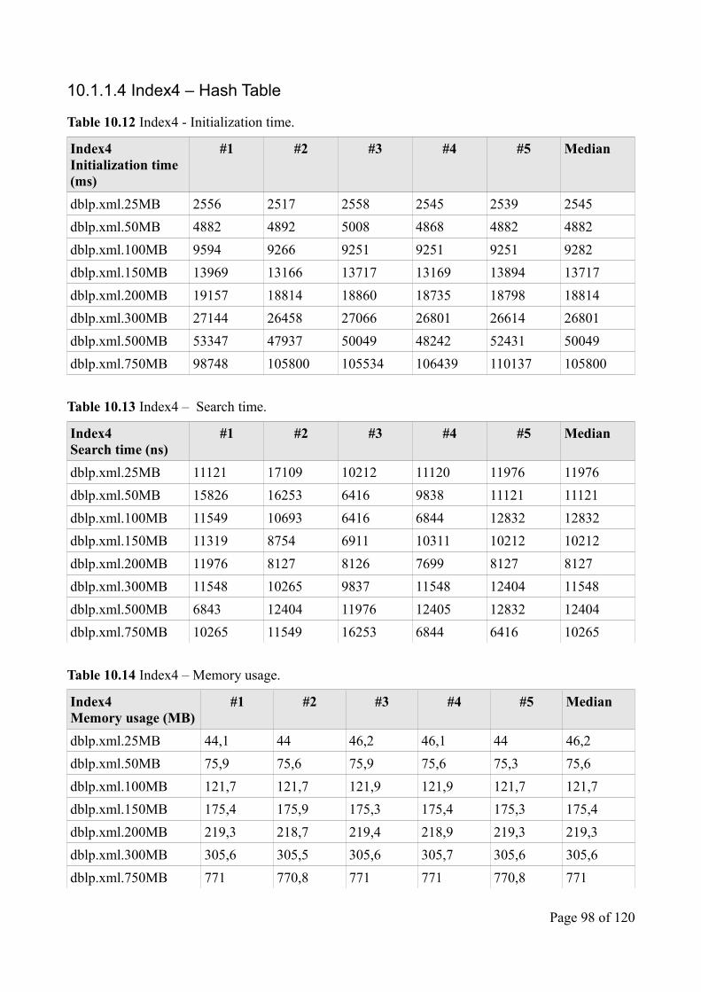
10.1.1.4 Index4 – Hash Table



#1 #2 #3 #4 #5 Median

dblp.xml.25MB 2556 2517 2558 2545 2539 2545dblp.xml.50MB 4882 4892 5008 4868 4882 4882dblp.xml.100MB 9594 9266 9251 9251 9251 9282dblp.xml.150MB 13969 13166 13717 13169 13894 13717dblp.xml.200MB 19157 18814 18860 18735 18798 18814dblp.xml.300MB 27144 26458 27066 26801 26614 26801dblp.xml.500MB 53347 47937 50049 48242 52431 50049dblp.xml.750MB 98748 105800 105534 106439 110137 105800

Table 10.13 Index4 – Search time.


#1 #2 #3 #4 #5 Median

dblp.xml.25MB 11121 17109 10212 11120 11976 11976dblp.xml.50MB 15826 16253 6416 9838 11121 11121dblp.xml.100MB 11549 10693 6416 6844 12832 12832dblp.xml.150MB 11319 8754 6911 10311 10212 10212dblp.xml.200MB 11976 8127 8126 7699 8127 8127dblp.xml.300MB 11548 10265 9837 11548 12404 11548dblp.xml.500MB 6843 12404 11976 12405 12832 12404dblp.xml.750MB 10265 11549 16253 6844 6416 10265



#1 #2 #3 #4 #5 Median

dblp.xml.25MB 44,1 44 46,2 46,1 44 46,2dblp.xml.50MB 75,9 75,6 75,9 75,6 75,3 75,6dblp.xml.100MB 121,7 121,7 121,9 121,9 121,7 121,7dblp.xml.150MB 175,4 175,9 175,3 175,4 175,3 175,4dblp.xml.200MB 219,3 218,7 219,4 218,9 219,3 219,3dblp.xml.300MB 305,6 305,5 305,6 305,7 305,6 305,6dblp.xml.750MB 771 770,8 771 771 770,8 771

of 120

10.1.1.5 Index5 – Title Search



#1 #2 #3 #4 #5 Median




#1 #2 #3 #4 #5 Median




#1 #2 #3 #4 #5 Median

dblp.xml.25MB 60,3 60,1 60,3 60,2 60,7 60,3dblp.xml.50MB 113,2 113,2 113,5 113,5 113,4 113,4dblp.xml.100MB 211,7 211,7 211,7 211,8 211,7 211,7dblp.xml.150MB 306,8 306,9 306,9 306,7 306,8 306,8dblp.xml.200MB 401,8 405,6 401,1 402,1 402,2 401,8dblp.xml.300MB 589,2 589,5 589,8 589,4 589,8 589,5

of 120

10.1.1.6 Index6 – Keyword Search

Table 10.18 Index6 - Initialization time. With stop word filter.


#1 #2 #3 #4 #5 Median


Table 10.19 Index6 – Initialization time. Without stop word filter.


#1 #2 #3 #4 #5 Median




#1 #2 #3 #4 #5 Median


of 120

Table 10.21 Index6 – Memory usage. With stop word filter.


#1 #2 #3 #4 #5 Median

dblp.xml.25MB 99,9 99,7 99,7 99,7 99,9 99,7dblp.xml.50MB 181,7 185,1 184,1 184,4 185,2 184,4dblp.xml.100MB 360,1 361,7 364,8 362 359,3 361,7dblp.xml.150MB 556,9 555,5 553,9 556,6 554,8 555,5dblp.xml.200MB 723,4 724,4 723,7 723,1 723,5 723,5dblp.xml.300MB 1034,4 1032,3 1055 1032,2 1056,5 1034,4

Table 10.22 Index6 – Memory usage. Without stop word filter.


#1 #2 #3 #4 #5 Median

dblp.xml.25MB 112,5 111 112,6 110,7 111,1 111,1dblp.xml.50MB 208,8 215 213,4 213,6 214,1 213,6dblp.xml.100MB 421 424,7 419,9 421 420,3 421dblp.xml.150MB 724,8 724,9 714,9 722,4 723,5 723,5dblp.xml.200MB 875,4 876 876,5 875,9 875,8 875,9dblp.xml.300MB 1417,2 1374,3 1299,6 1265,3 1230,4 1299,6

of 120

10.1.1.7 Index7 – Prefix Search

10.1.1.7.1 Sorted List

Table 10.23 Index7 – Sorted list Initialization time.


#1 #2 #3 #4 #5 Median


Table 10.24 Index7 – Sorted list prefix search time.

Index7 Prefix Search time (ns)

#1 #2 #3 #4 #5 Median


Table 10.25 Index7 – Sorted list full search time.Index7 Full search time (ns)

#1 #2 #3 #4 #5 Median


of 120

Table 10.26 Index7 – Sorted list memory usage.

Index7Memory usage (MB)

#1 #2 #3 #4 #5 Median

dblp.xml.25MB 96 95,8 95,2 96,2 95,8 95,8dblp.xml.50MB 179,8 180,1 180,1 180 177,9 180dblp.xml.100MB 356,1 357,1 356,6 355,9 357,2 356,6dblp.xml.150MB 556,4 552,1 553,3 554,6 552,8 553,3dblp.xml.200MB 731,4 740,9 736,4 731,2 731,4 731,4dblp.xml.300MB 1055,2 1033,5 1054 1037,2 1037 1037,6

10.1.1.7.2 Ternary Search Tree

Table 10.27 Index7 – Ternary search tree initialization time.


#1 #2 #3 #4 #5 Median


Table 10.28 Index7 – Ternary search tree prefix search time.Index7 Prefix Search time (ns)

#1 #2 #3 #4 #5 Median


of 120

Table 10.29 Index7 – Ternary search tree full search time.Index7 Full search time (ns)

#1 #2 #3 #4 #5 Median


Table 10.30 Index7 – Ternary search tree memory usage.


#1 #2 #3 #4 #5 Median

dblp.xml.25MB 122,2 124,4 124,8 124,6 124,2 124,4dblp.xml.50MB 231,1 224,2 225,5 230,4 231,6 230,4dblp.xml.100MB 434,7 435,7 434,7 434,7 435,2 434,7dblp.xml.150MB 668,8 657,7 651 652,1 668 657,7dblp.xml.200MB 866,3 865,2 862,2 865,1 863,4 865,2dblp.xml.300MB 1235,3 1234,3 1247 1231,2 1249,6 1235,3

10.1.1.7.3 Red-black Tree

Table 10.31 Index7 – Red-black tree initialization time.


#1 #2 #3 #4 #5 Median


of 120

Table 10.32 Index7 – Red-black tree prefix search time.Index7 Prefix Search time (ns)

#1 #2 #3 #4 #5 Median


Table 10.33 Index7 – Red-black tree full search time.

Index7 Full search time (ns)

#1 #2 #3 #4 #5 Median


Table 10.34 Index7 – Red-black tree memory usage.


#1 #2 #3 #4 #5 Median

dblp.xml.25MB 100,2 97,5 97,8 98 97,8 97,8dblp.xml.50MB 193,2 190,3 187,1 192,4 188,3 190,3dblp.xml.100MB 412,2 411,1 413,3 418,2 419,4 413,3dblp.xml.150MB 605 606,7 590,7 589,2 603,3 603,3dblp.xml.200MB 866,9 866,4 863,7 811,8 799,7 863,7dblp.xml.300MB 1173,2 1167,8 1204,5 1203,5 1172,7 1173,2

of 120

10.1.1.8 Index8Table 10.35 Index8 Integer Array – Initialization time.


#1 #2 #3 #4 #5 Median

dblp.xml.25MB 13369 13197 13229 13369 13166 13229dblp.xml.50MB 41630 40922 41221 41522 41884 41630dblp.xml.100MB 132834 132990 132693 133598 132678 132834dblp.xml.200MB 525017 527023 517515 512112 515519 517515dblp.xml.300MB 1036060 1031832 1031536 1022689 1079366 1021832dblp.xml (750MB) 9409690 9500325 9411134 9476512 9446740 9446740

Table 10.36 Index8 Integer Array – Memory usage.Index8Memory usage (MB)

#1 #2 #3 #4 #5 Median

dblp.xml.25MB 102,5 102,6 102,4 102,5 102,5 102,5dblp.xml.50MB 201 197,2 196,1 197,2 197,3 197,2dblp.xml.100MB 298,4 345,4 348,8 345,4 345,5 345,4dblp.xml.200MB 704,3 710,8 707,2 704,4 704,4 704,4dblp.xml.300MB 924,4 919,2 919,1 919,2 919,7 919,2dblp.xml (750MB) 2181,3 2159,4 2149,7 2157,6 2167,1 2159,4

of 120

10.1.1.9 Index9 – Boolean SearchTable 10.37 Index9 – Boolean search time. Searching for publications using the queries “algorithm” and “fast”.Index7 Prefix Search time (ns)

#1 #2 #3 #4 #5 Median


of 120

10.1.2 Functional test - screen shots

10.1.2.1 Index1

10.1.2.2 Index2

of 120

Figure 10.1 Index1 – Screen shot

Figure 10.2 Index2 - Screen shot

10.1.2.3 Index3

of 120


10.1.2.4 Index4

of 120


10.1.2.5 Index5

of 120


10.1.2.6 Index6

of 120


of 120


10.1.2.7 Index7

of 120



10.1.2.8 Index8

of 120

Figure 10.10 Index8 - Screen shot. Prefix search test

Figure 10.11 Index8 – Screen shot. Printout of publication objects and their list of authors

of 120

Figure 10.12 Index8 – Screen shot. Printout of the author objects and their list of publications.

10.1.2.9 Index9

of 120

Figure 10.13 Index9 – Screen shot. Boolean search using keywords.

Figure 10.14 Index9 – Screen shot. Boolean search using nameparts.

Figure 10.15 Index9 – Screen shot. Boolean search using authorIDs.

10.1.2.10 Index10

of 120

Figure 10.16 Index10 – Screen shot. Auto-suggest menu test on authors.

Figure 10.17 Index10 – Screen shot. Auto-suggest menu test on publicationa.

Figure 10.18 Index10 – Screen shot. Look up page.

Figure 10.19 Index10 – Screen shot. Search results for a boolean search using keywords.

of 120

Figure 10.20 Index10 – Screen shot. Search results for a boolean search using author IDs.

10.3 Stop Words

Table 10.38 Stop words in ascending order

about

after

all

am

an

and

any

are

as

at

be

because

been

before

but

by

can

cannot

could

did

do

does

eg

else

for

from

get

go

got

had

has

have

he

hence

her

here

hereby

hers

his

how

ie

if

in

into

is

it

its

let

me

my

nor

not

now

of

often

on

one

or

our

put

should

so

than

that

the

their

them

then

there

these

they

this

thus

to

too

us

we

were

what

where

when

which

with

who

would

yet

you

your

yours

of 120

search engine project - dtu electronic theses and ...etd.dtu.dk/thesis/271698/dip10_46.pdf ·...

Documents