scottish urban air quality steering group - modelling & monitoring workshop - scott hamilton

© Ricardo-AEA Ltd

www.ricardo-aea.com

Ricardo-AEA

Dr Scott Hamilton, Technical Lead in Urban Scale Dispersion Modelling, Ricardo-AEA

Local, regional, national approaches used by Ricardo-AEA in recent years, and some recent developments

Modelling and monitoring- UK consultancy view

© Ricardo-AEA Ltd Ricardo-AEA in Confidence 2

• Local dispersion modelling approaches for road traffic sources in the UK

• Ricardo-AEA’s work for UK/DAs under the EU Air Quality Directives

• National modelling- the PCM model

• Recent open source city scale modelling developments at Ricardo-AEA

In this session….


In the UK why do we model air quality?

• Local assessments of air pollution – Local Air Quality Management – Planning applications – Permitting

• City scale assessments – LEZ schemes – Health studies

• National scale – Compliance reporting to Europe – PCM suite of models


Commonly applied models in the UK - influence of scale

• Local – ADMS-Roads, ADMS, AERMOD

• Urban – ADMS-Urban, GIS-AERMOD,

CMAQ, CALPUFF

• National – CMAQ


Some questions we ask ourselves when modelling…..

•What question am I trying to answer?

•What gap am I trying to fill? Should I even run a model? Would measurements be better?

•How big is the area I want to model, how many sources and how many prediction points do I want?

•How complex are my sources? If they’re complex do I have enough detail in the input data to derive concentrations at my desired resolution?

•How will I treat the “meteorological boundary conditions” to my model?

•Other air pollution sources are always very important, how will I derive the “chemical boundary conditions” to my model?

•How will I assimilate measured values to check my model performance? What do I mean by “good” model performance? How will I deal with model error?

•Is my model capable of answering the questions I want answered?


How do local dispersion models in the UK work?

•Simplified picture of reality (very!)

•Almost all operational models used in the UK are based on the Gaussian equations

•We’ve been using Gaussian models for many years. These are empirically driven but they work well. They cope with the variable and random pattern of pollutant density within turbulent plumes by estimating a smoothed plume shape by averaging the “patchiness” over time.

•Even “advanced” or “next generation” models like ADMS and AERMOD are Gaussian formulations with some modifications

•All models currently used in the UK for statutory applications have been validated for their intended application.


UK typical road traffic dispersion modelling methods

Different ways to model urban dispersion- increasing in complexity….

Screening model – Simple model like DMRB,

completely empirical

Gaussian model – dispersion mainly as a

function of distance and basic meteorology- semi-

empirical

Computational Fluid Dynamics - solution based on numerical

treatment of fluid flow. Complex and time/expertise intensive

Gaussian models don’t normally “pair” well with observations in

time and space. Good for annual means and finding maxima used as the basis of regulation. Cannot

model calm conditions.

CFD models like Envi-Met are useful for looking at the influence of buildings

on flow- but they can only treat one met condition at a time and still cannot

be considered “practical” models for local air quality studies (8760 met

conditions per year!)

Just because we can run complex models doesn’t mean we should…

Annual mean calculations primarily, treatment of shorter

averages done using empirical functions.

© Ricardo-AEA Ltd Ricardo-AEA in Confidence 8 8

Source characterisation- road traffic

Emissions from road traffic are variable according to the behaviour and make up of the fleet- we need to answer some questions to assess the impact… •How many vehicles per day? •How fast is the traffic moving? •What is the split of light and heavy vehicles? •Are more detailed fleet splits available? •Are there any areas of congestion or stationary traffic? •Currently (necessarily) most studies use basic treatments of traffic conditions. USEPA has some good guidance and methods (drive cycles, MOVES)

What we want to achieve from modelling will influence how detailed the datasets listed above are. Its no use trying to model hourly scale if we don’t know these parameters at the same temporal

resolution.

We normally only model annual mean concentrations when dealing with road traffic emissions….


• Calculate emissions – Emissions factor toolkit (or model can do this)- or use COPERT IV, or other approved emission factor

tool. Traffic activity from variety of sources, DfT, Transport Scotland, Count data – If working on NO2 we calculate NOx emissions

• Predict concentrations at receptors and wider area – Using a validated/peer reviewed dispersion model – Use good meteorological data (it has errors too) – Locate receptors appropriately

• Add background concentrations – gives total concentration

• Calculate final pollutant concentrations – If working on NO2 convert from total NOx to NO2

• Verify against monitoring data – do the model outputs agree or is a correction needed?

• When model agreement is good, plot data in GIS – Software interpolates between model predictions to give contour plots

• Answer question we set out to address • Are there exceedances of a standard, what is their magnitude

“Usual” LAQM.TG(09) approach to modelling concentrations from traffic


Example- Concentrations of PM10 with several areas of exceedence

Note: PM10 models are always much more uncertain, mainly due to the lack of measurements for validation purposes

Typical study, are there exceedances of standards? If there are the Local Authority has an obligation under the Environment Act 1995 to declare an AQMA and prepare an Action Plan.


Model verification •Essential part of the process- the reality check!

•In local models for road traffic its almost always a comparison between annual mean measured Vs modelled values

•For NO2 we verify the road contribution to NOx concentrations predicted by our model

•We derive an adjustment factor based on model divergence at several monitoring locations- the model often under or overpredicts

•We then apply the adjustment to the modelled predictions and add to our local background

•Calculate NO2 from NOx to get our final predictions and estimate model error (e.g. calculate Root Mean Square Error)

•PM10 is usually verified using fewer monitoring locations (no cheap, simple monitor for PM10)


Calculating model error- the TG(09) method The root mean square error can be used to estimate overall model error- TG(09) requires a RMSE value less than 10% of the annual mean objective under consideration. In practice this means that when working with the NO2 annual mean objective, our model can carry an error of 4 ugm3 and still be accurate enough for LAQM purposes.

Subtract modelled from measured for each location and square the result Take the average of all the squared errors and take the square root of that value- this is the RMSE The units are the same as the measurements/model results This value broadly reflects model uncertainty. This is why some Councils choose to declare AQMAs slightly larger than necessary


What about other sources?

13 Slide:

•If you have a large study area you’ll need to either model other sources discretely or use background values to represent them (be careful about double counting)

•Top image- individual properties in a domestic combustion study are the “dots”

•Summed into area sources and run in ADMS. •Modelling roads nearby in isolation without addressing the domestic sector would have been pointless

•Transboundary sources are also very important for PM10- modelling short term averages for PM would be extremely difficult (depending on the wind direction!)

•There’s a significant UK and European evidence base on other sources, but they are ALL based on annual average emissions.


National scale programmes we run

14 Slide:

• Ricardo-AEA have been providing the UK and Scottish Governments with their main air quality evidence bases for several decades- we were part of the civil service (Warren Springs, UKAEA, AEA, Ricardo-AEA)

• The National Atmospheric Emissions Inventory is the official emissions database for the whole UK.

• The Automatic Urban and Rural Network is used to measure compliance with Limit Values in the ambient air Directives. We do the QA/QC and run the database and website (UK-AIR, plus Scottish Government database)

• The Pollution Climate Mapping model is used to report to the European Commission on compliance with air quality Limit Values. It is the only model that can be used for compliance reporting by Government.

• For example- the PCM model uses mapped emissions estimates from the NAEI, and uses measurements from the AURN for validation purposes.


Ricardo-AEA websites for Government clients

This is the outward facing aspect of our work that spans >40 years in and for Government


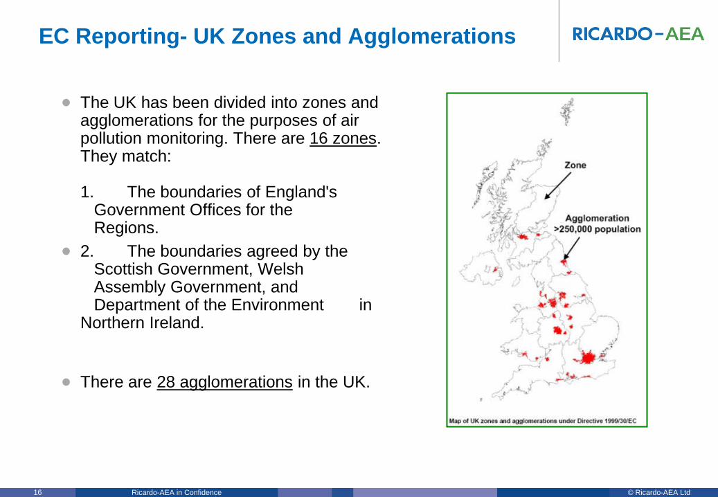
EC Reporting- UK Zones and Agglomerations

• The UK has been divided into zones and agglomerations for the purposes of air pollution monitoring. There are 16 zones. They match: 1. The boundaries of England's Government Offices for the Regions.

• 2. The boundaries agreed by the Scottish Government, Welsh Assembly Government, and Department of the Environment in Northern Ireland.

• There are 28 agglomerations in the UK.


Monitoring in the AURN

The Automatic Urban and Rural Network (AURN) is the UK's largest automatic monitoring network and is the main network used for compliance reporting against the Ambient Air Quality Directives. It includes over 100 automatic air quality monitoring stations measuring oxides of nitrogen (NOx), sulphur dioxide (SO2), ozone (O3), carbon monoxide (CO) and particles (PM10, PM2.5). Measurements must be taken using a reference method, or an equivalent method. These sites provide high resolution hourly information which is communicated rapidly to the public, using a wide range of electronic, media and web platforms.


Monitoring in Scotland

In addition to the AURN there is a Scottish network of 87 sites Data is subject to the same QA/QC as the AURN so is of very high quality www.scottishairquality.co.uk


Modelling for Directive reporting- the PCM model • The Pollution Climate Mapping (PCM) model is a

collection of models designed to fulfil part of the UK's EU Directive requirements (annual)

• Developed and maintained by Ricardo-AEA for the UK Government.

• The EU Air Quality Directive permits Member States to assess compliance using monitoring of air pollutant concentrations, supplemented by modelling

• The use of modelling to supplement monitoring will, in general, cover more of the territory of a Member State in those zones and agglomerations, and will therefore tend to reveal higher areas of exceedance of thresholds than information derived purely from monitoring

• The models supplement the AURN which, on its own doesn’t have enough sites to satisfy the Directive

• Its not designed for local application.


UK Ambient Air Quality Assessments

• Modelling for Air Quality Directive and 4th Daughter Directive reporting and policy assessments Mapping current concentrations Baseline & scenario based projections Health impact assessment for scenarios

• Policy Advice to Defra and the DAs Brings together information from

ambient measurements, emission inventories and models

• Models GIS-based PCM models


http://uk-air.defra.gov.uk/data/gis-mapping

User can download datasets from the PCM model using the data selector options on the Defra website we run.


PCM GIS-based models • Pollutants

– Air Quality Directive: SO2, NOx, NO2, PM10, PM2.5, Pb, C6H6, O3

– 4th Daughter Directive: BaP, As, Cd, Ni

• Maps built up from many layers – Regional (interpolated from rural

measurements) – Point sources modelled using dispersion

model – Area sources modelled using a dispersion

kernel approach – Roadside increment model

• Calibrated using automatic monitoring data from the AURN

• 1 km grid resolutions + urban major road links


PCM GIS-based model layers

• Layer 1: Regional background – Exact input data and method used depends

on pollutant

– Input data includes • Rural measurements of NOx and NO2, Cl • EMEP for secondary inorganic aerosol

emissions sensitivity coefficient (for PM projections)

• TRACK model outputs for regional primary PM

• NAME aerosol outputs


PCM GIS-based models • Layer 2: Point sources

– Input data: • NAEI point sources database • Point sources stack parameter information held by

PCM team (only updated on an ad hoc basis) • Met data

– Large point sources (annual emission exceeds a pre-defined threshold) • Emissions data and stack parameters processed in

PCM point sources database • Modelled explicitly in ADMS • For 2011 mapping >1000 individual point sources

modelled

– Small points (annual emission less than the pre-defined threshold)

– Outputs • 1km x 1km grid of concentrations resulting from

point source emissions for each pollutant


PCM GIS-based models

• Layer 3: Area sources – Input data

• 1km x 1km emissions maps • Emissions projections • Met data • AURN monitoring data

– Method • Dispersion of unitary emission calculated

– road traffic, domestic and other sources – Inner conurbations, cities/towns and else where

• Relevant kernel applied to each UK grid square to calculate concentrations within the square for each pollutant

• Calibrated using AURN monitoring data

– Outputs • 1km x 1km grid of concentrations resulting from area

source emissions for each pollutant



• Layer 4: Other pollutant specific layers

• Examples – Re-suspended PM (soils and vehicles)

• Input data – land cover map for initial PM map – soil composition data to calculate map for heavy metals – vehicle activity

– Fugitive emissions of benzene from point sources



• Layer 5: Roadside increment model – Input data

• Road link mapped emissions data from the NAEI • Data on road type, vehicle flows for each

individual road link • AURN monitoring data

– Method • Empirically based approach (similar to DMRB) • Applies adjustment to emission depending on

traffic flow to account for different factors that influence dispersion

• Calibrated using AURN monitoring data

– Outputs • Concentration estimates for each of ~9000 road

links included in the model

0

10

20

30

40

50

60

70

0 10 20 30 40 50 60 70Measured NO2 (µg m-3)

Mod

elle

d N

O2 (

µg m

-3)

National NetworkVerification Sitesx = yx = y + 30%x = y - 30%


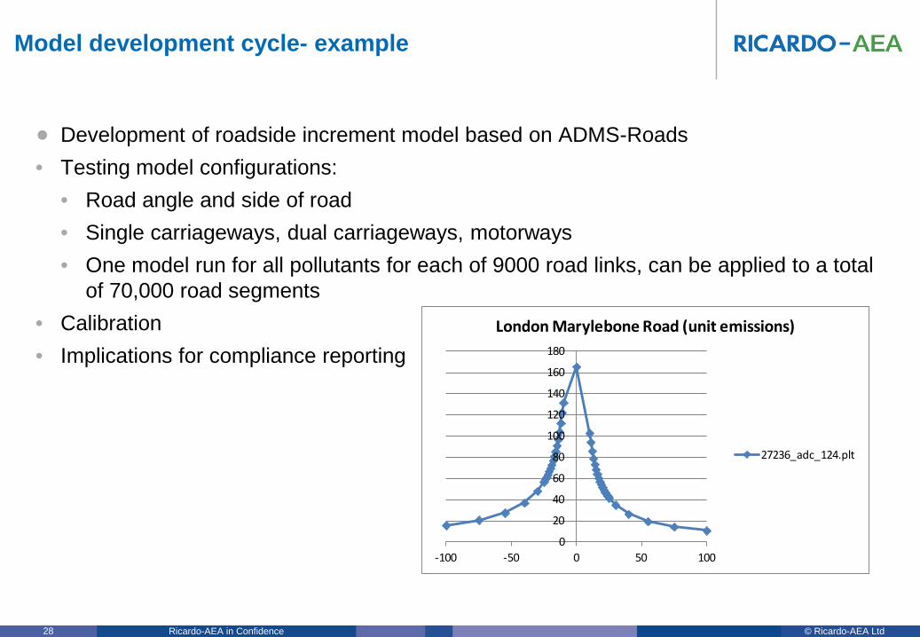
Model development cycle- example

• Development of roadside increment model based on ADMS-Roads • Testing model configurations:

• Road angle and side of road • Single carriageways, dual carriageways, motorways • One model run for all pollutants for each of 9000 road links, can be applied to a total

of 70,000 road segments • Calibration • Implications for compliance reporting

0

20

40

60

80

100

120

140

160

180

-100 -50 0 50 100

London Marylebone Road (unit emissions)

27236_adc_124.plt


NOx and NO2 in 2011

Background NOx Background NO2 Regional NOx Roadside NO2


PCM GIS-based models: outputs

• GIS maps • Base year and projections

– Background 1 km x 1 km – Roadside ~ 9000 urban road links

• Background and roadside exceedance statistics – By zone

• Population-weighted mean background concentration – For health impact assessment, CBA

• Source apportionment – To support policy development – Development of air quality plans – LAQM


Annual reporting


PCM model performance

Defra urban model evaluation analysis – Phase 1- http://uk-air.defra.gov.uk/assets/documents/reports/cat20/1105091516_UrbanFinal.pdf

http://uk-air.defra.gov.uk/assets/documents/reports/cat20/1105091516_UrbanFinal.pdf


City scale modelling developments (project driven)

• Working towards a more “open source” way of operating (the way the world is headed)- using USEPA modelling codes which have broad international acceptance

• USEPA AERMOD dispersion “kernels” in a GIS environment- massive savings in run time compared with standard models for city scale assessments

• We’ve been using such models at Ricardo-AEA for many

years, groups at Kings College and Imperial College using similar techniques in London

• The use of AERMOD to derive dispersion kernels means there is no need for licences- GIS is the only cost, for now

• The technique takes the USEPA Hotspot Analysis guidance and scales it up to model entire cities very quickly and efficiently (tried and tested!)


Technical challenges for the Riyadh integrated dispersion model (roads focus)

• Riyadh is a very large city- we are modelling more than 3000km2, Greater London is 1573km2.

• Model run times are unmanageable using conventional techniques

• We still need to achieve a high level of detail but it should run efficiently on standard IT and GIS systems and be updateable to support future modelling efforts

• It should use open source software (other than ArcGIS)

• The model will be coupled to CMAQ for regional concentrations and perhaps WRF for forecasting

• We’ve achieved all this at 8m resolution and we’ll be installing the system on our clients’ GIS systems soon

• The use of prognostic met data means we can “extract” virtual stations across a wide area and use the data in the model

Riyadh model domain


Detailed road geometries, from EMME traffic model

Accompanying model report also has fleet split (very basic) and road categorisation.


GIS-AERMOD- dispersion kernels

200m

8m resolution

440m

40m resolution

2.2km

200m resolution

11km

1000m resolution

55km

The fine resolution grids characterise dispersion of emissions from roads close to the receptor

The coarse resolution grids provide a background concentration from roads further away- of course in an hour emissions can’t travel this far this fast under a Gaussian formulation but we can live with that

Not to scale

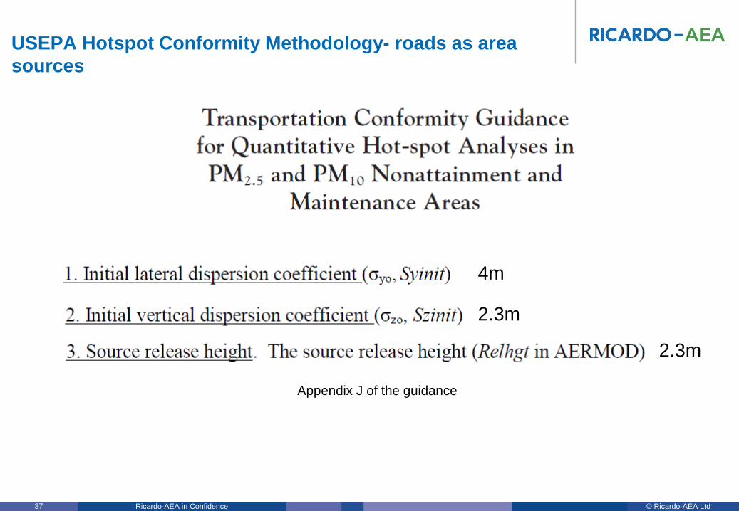
Kernels are set up to closely align with the USEPA method for modelling road traffic in their Hotspot Conformity Analysis guidance- specifies release height for the area source for example


USEPA Hotspot Conformity Methodology- roads as area sources

4m

2.3m

2.3m

Appendix J of the guidance


GIS-AERMOD Vs ADMS Roads in the near field

ADMS Roads GIS-AERMOD

Results are similar across the grid for both models. The graph shows points within 16m of the roadside along the east to west link, disregarding concentrations on the road surface. RMSE= 3ugm3

Same symbology for both models


1m roughness concentration transects

Red line is a transect through the whole domain, graphs show concentrations along the line

Blue= GISAERMOD Red= ADMS

Roads


Riyadh emissions calculations

• All emissions calculated (COPERT) in the GIS (ArcMap or QGIS)

• 11,000km of roads (21,000 links) populated in <2min

• No need to do any geoprocessing in Excel or Access

EMEP Guide 2013

EF = (a + c * V + e * V²)/(1 + b * V + d * V²)

Petrol Car Euro 2


GIS-AERMOD Dispersion plots

ArcMap

Google Earth


GIS-AERMOD- development in Riyadh- demo runs

• Up to 137,000,000 individual predictions • About 415,000,000,000 calculations in ArcGIS • Run time in ArcGIS for the road model is about 10 to 40 minutes currently for

the entire Riyadh urban area (including a lot of desert) • Model resolution is good enough to tell us pollutant concentrations at

individual properties in the city so we can tie this data to health stats later if need be.

• Every prediction cell contains a contribution from every major road in the city • Emission estimates could come from any emissions model derived from any

traffic model, as long as they are hourly averages • Can operate at any temporal resolution (1hr to 10years!)- with NO uplift in

run times in the GIS environment- though kernels will take longer to prepare.

Whole city (8m resolution) District of city Street level plot


London GIS-AERMOD model- traffic NO2 2013

• Leverages existing government datasets • LAEI 2010 traffic data • Flow, composition and speed • 2013 emission factors derived from COPERT

IV • Non-road concentrations from Defra LAQM

maps (the PCM model we develop) • NOx calculated in the GIS model in about 90

secs, dispersion fields with empirical NO2 conversion in 5 minutes (8m resolution)

• Scenario tests in a few minutes


London GIS-AERMOD model- agreement at AURN sites

• NO2 annual mean concentrations

• Comparison with London AURN measured values in 2013

• The model “as is” underpredicted somewhat- reasons unclear (could be emission factors, traffic activity data, empirical NO2 function etc etc)

• In general, after accounting for systematic underprediction, the model does a good job

• RMSE value of 4.4μgm3

• I’m working on a validation paper for a peer reviewed journal at present. The results shown here will be included


Google Earth example with 3D building models


Thanks for listening.

• Any Qs?

© Ricardo-AEA Ltd

www.ricardo-aea.com

T: E: W:

Ricardo-AEA Ltd The Gemini Building Fermi Avenue Harwell, Didcot, OX11 0QR

Dr Scott Hamilton

01235 753 716 [email protected] www.ricardo-aea.com

scottish urban air quality steering group - modelling & monitoring workshop - scott hamilton

Environment

ricardoaea local

ricardoaea dr scott

uk ricardoaeas work

screening model simple

model capable

model error

local dispersion models

good model performance