Page 1 of 12      

Scintillation of Light from Distant Objects due to Anisotropic and Non-Kolmogorov Turbulence

Richard B. Holmes Boeing LTS, 535 Lipoa Parkway, #200, Kihei, HI 96753

V.S. Rao Gudimetla Air Force Research Laboratories, Directed Energy Directorate, Det 15, 535 Lipoa Parkway, #

200, Kihei, HI 96753 Jacob Lucas

Boeing LTS, 535 Lipoa Parkway, #200, Kihei, HI 96753 Jim F. Riker

Air Force Research Laboratories, Space Vehicles Directorate, 3550 Aberdeen Avenue SE, Kirtland AFB, NM 87011

ABSTRACT

Observations at AMOS and elsewhere suggest that turbulence is sometimes non-isotropic and non-Kolmogorov in nature. Such turbulence can produce different jitter, wavefront error, and scintillation than expected from isotropic Kolmogorov turbulence. These differences can impact the design of sensor systems that must see through this atypical turbulence. Quantitative definitions are provided for anisotropic turbulence and non-Kolmogorov turbulence. Using previously developed analyses and with extensive simulations for a plane wave, corresponding to light from a satellite or star, results are presented that parametrically show how scintillation differs from that of standard Kolmogorov turbulence, under a variety of conditions. Also included are conditions appropriate for observations of sources on Mauna Loa as seen at AMOS.

1. INTRODUCTION

Researchers at the Air Force Maui Optical Site (AMOS) have reported that atmospheric turbulence as measured by optical observations does not always fit the conventional model of isotropic turbulence with an 11/3 spatial frequency power law [1-5]. Earlier measurements indicated that anisotropy may occur near the surface of the earth [6, 7]. Other measurements have indicated that non-Kolmogorov turbulence is present in the troposphere [8-9]. At higher, altitudes, in the stratosphere, turbulence that is layered, anisotropic and non-Kolmogorov has been reported [10-11]. These and other measurements suggest that such turbulence is not infrequent, and that there are physical reasons for non-Kolmogorov turbulence to persist in some situations.

Models have been developed in the past for forms of anisotropic or non-Kolmogorov turbulence. These models include those proposed by Gurvich et. al. [12], Aleksandrov et. al. [13], Antoshkin et. al. [14], and Ostachev et. al. [15]. These models for turbulence then can be used to estimate scintillation by applying the first-order Rytov theory [15-23]. This is done below, with closed -form expressions for both non-Kolmogorov and non-isotropic conditions. Give the possibility that the analysis may be imperfect and experiments are difficult, a simulation is performed to verify the analysis and explore the limitations of the Rytov analysis. This simulation uses the same split-operator technique used by others in the [24-26]. This simulation technique uses Fresnel propagation, which is more general and accurate than the Rytov approximation, so can explore the limits of the analytic expressions. The analysis and simulation are applied to plane wave propagation through the atmosphere, as might arise from light from distant objects. The theory applies well for objects that are 250 km or more in range from the AMOS Haleakala site, at zenith angles up to 60 degrees.

Page 2 of 12      

Section 2 discusses the basic model chosen for non-isotropic, non-Kolmogorov turbulence. Section 3 applies the model in the Rytov paradigm to develop an expression for the log-amplitude correlation function along a path with constant turbulence strength. These analytic results are used to test the wave optics simulation, in Section 4. Section 5 then applies the validated simulation to AMOS conditions. Section 5 summarizes the analysis and simulation results.

2. Model for Anisotropic, Non-Kolmogorov turbulence

The Kolmogorov spectrum for refractive index has an exponent of 11/3:

( ) 6/1122033.0)( −=Φ KCK n (1)

Where K2 = Kx2 + Ky

2 + Kz2, and Cn

2 is the refractive-index structure constant. Past work on non-Kolmogorov turbulence indicates that the exponent α=2·11/6 must be between 3 and 5 in order to obtain a meaningful refractive-index structure function, and between 3 and 4 for a useful optical-wave structure function [22, 23]. Generalizing to non-Kolmogorov exponents and to anisotropy, one has

( ) 2/222222/)()()( ααβα−

++=Φ zyx KKbKaabAK (2)

where )(αA is the generalization of the value of 0.033 for non-Kolmogorov exponents, β  is the generalization of

the refractive index structure constant Cn2 for non-Kolmogorov exponents, and a and b are anisotropy factors. The

factor A(α) is given by

A(α) = Γ(α -1)*sin[(α-3)π/2]/(4π2), (3)

and the factor 2/)( αab is needed to conserve energy in the turbulent medium relative to the isotropic case. One

may simplify Eq. (2) a bit more by setting a = 1 and b2 = 1+ε2, without loss of generality. Using Ky = Ksin(θK), one then has [24, 25]

( ) 2/224/2 )(sin1)1()()( ααα θεεβα−− ++=Φ Kn KAK (4)

This is the expression used for anisotropic non-Kolmogorov turbulence in the following sections.

3. ANALYSIS OF SCINTILLATION

Given expression (4) from the preceding section for the refractive index power spectrum, one may apply the Rytov approximation to the wave equation to obtain the following general expression for the log-amplitude correlation function in plane-wave propagation [24-25]:

( )

( ) 2/22

)cos(2

0

221

0

4/2

0

2

2/222

224/2

0

2

)(sin11sin)1()()(

)(sin1sin)1()()(),(

α

θθρπ

αα

ααραρχ

θεθεαβπ

θεεαβπθρ

ρ

K

iKK

L

KiK

L

KedkLKKdKAzdzk

KkLKeKdAzdzkB

+⎥⎦

⎤⎢⎣

⎡+=

+⎥⎦

⎤⎢⎣

⎡+=

−+−∞

−−•

∫∫∫

∫∫

(5)

Page 3 of 12      

where  Bχ(ρ, θρ) is the log-amplitude correlation function as a function of separation ρ and angle θρ with respect to an axis perpendicular to the line of site, k is the optical wavenumber, 2π/λ, β(z) is the turbulence strength along the path parameterized by z, A(α) is a normalization factor that depends on Kolmogorov exponent ε is the anisotropy, K is the spatial wavenumber of the aberrations, L is the path length, and θK is the angle that K makes with the anisotropy axis. Note that this expression allows for the turbulence strength, the anisotropy, and the Kolmogorov exponent to vary along the path. Simplifying to the case in which these are constant along the path, including turbulence strength β(z), one can write

( )

( ) 2/22

)cos(2

0

2

21

0

4/22

2/222

22

4/22

)(sin11sin1)1()(

)(sin1sin1

)1()(),(

α

θθρπ

αα

ααρ

αρχ

θεθεβπα

θε

εβαπθρ

ρ

K

iKK

KiK

KedkLK

LKkKdKLkA

KkLK

LKkeKd

ALkB

+⎭⎬⎫

⎩⎨⎧

⎥⎦

⎤⎢⎣

⎡−+=

+⎭⎬⎫

⎩⎨⎧

⎥⎦

⎤⎢⎣

⎡−

+=

−+−∞

−−•

∫∫

∫ (6)

Expanding the inner-most term of the anisotropy into a power series and performing the integrations over K and θK for each term of the power series, one obtains

[ ]

[ ]bmammm

m

mbmamm

QQQmFmLkA

QQQFLkAB

2212

1

12/1122/2/3

0221212/1122/2/3

),,()2cos()1()1())((

),,0()1()(5.0),(

−−−++

−−+=

∑∞

=

−

=−

αεθεβπα

αεεβπαθρ

ραα

ααρχ

(7)

In this equation, F(m,ε2, α) is defined by

( ) 2/22

2

)(sin1

)2cos(),,(α

π

π θε

θθαε

K

KK

mdmF+

= ∫+

−

      (8)

and the expressions for Qm1, Qm2a, and Qm2b are developed using Mellin transforms, and are as follows:

⎥⎦

⎤⎢⎣

⎡

+++

+−+−Γ⎟

⎠

⎞⎜⎝

⎛= −−−

2/32/14/2/4/2/14/2/2/14/2/

28

12/12/

21 αα

ααπρ α

α

mmmm

LkQm (9)

⎪⎭

⎪⎬⎫

⎪⎩

⎪⎨⎧

⎟⎟⎠

⎞⎜⎜⎝

⎛⎟⎠

⎞⎜⎝

⎛−++−+−

⎥⎦

⎤⎢⎣

⎡

−+++

+−Γ⎟

⎠

⎞⎜⎝

⎛= ∑∞

=

−−

22

32

2

0

12/2

8;1,2/1,2/1;4/2/,2/14/2/

2/14/12/12/12/14/2/

82

ραα

α

αρπα

LkmmmmF

mmmm

LkQ

m

mam

(10)

Page 4 of 12      

⎪⎭

⎪⎬⎫

⎪⎩

⎪⎨⎧

⎟⎟⎠

⎞⎜⎜⎝

⎛⎟⎠

⎞⎜⎝

⎛−+++−+−

⎥⎦

⎤⎢⎣

⎡

−+++

−+−Γ⎟

⎠

⎞⎜⎝

⎛=+

−−

22

32

1212/

2

8;2/3,1,2/3;2/14/2/,14/2/

2/2/14/2/312/114/2/

82

ραα

α

αρπα

LkmmmmF

mmmm

LkQ

m

bm

(11)

In the above equations, the multi-argument gamma function refers to a ratio of products of single-argument gamma functions, so for example,

)()()()()()(fedcba

fedcba

ΓΓΓ

ΓΓΓ=⎥

⎦

⎤⎢⎣

⎡Γ

(12)

Evaluation of Qm1 is direct but the evaluations of Qm2a and Qm2b need the poles of the integrand, which are located at

...02/14/....2,1,02/12/

.....2,1,02/

33

22

11

=−−=

=++=

=+=

nwithnsnwithnms

nwithnms

α (13)

It follows from the above at zero separation that the generalized Rytov variance is

( ) ( )( ) [ ] [ ] 4/22/)2/3(2/5)2/1(2 )1(4//4/)2(2/, αααα εααπβααεασ +Γ−Γ−= −− LkAR (14)

The above expressions involve a sum of a series of products of hypergeometric and gamma functions that prove to be convergent in cases of interest.

4. COMPARISON OF ANALYSIS AND SIMULATION

The above expressions for plane waves in turbulence of uniform strength are compared to detailed wave optics simulations. The simulations utilize grids consisting of 1024 × 1024 points, with the usual split-operator approach [26-28] that combines phase screens with Fresnel propagation between screens. It is found that a grid point spacing of 5 mm gives good accuracy and provides large separations for the correlation function. The phase screens are created using the well-known approach [26] involving random, statistically independent Fourier components, but with anisotropy and a non-Kolmogorov exponent included, as outlined above. For the comparison cases shown herein, 61 propagation steps are used, with 60 phase screens. This proves to be adequate for convergence in all cases considered, for ranges up to 100 km. The propagations are performed with “wrapped” boundary conditions, which works well when both the phase screens and the propagations are fast-Fourier-transform-based, as they are here. Three time steps with large temporal spacing are used to reduce the variance in the simulation-based estimate of the log-amplitude correlation function. The following figures in this section all show a comparison of the wave optics simulation and the analytical log-amplitude correlation for uniform turbulence. A wavelength of 0.737 µm is used in this section. For the first four figures, a range of 100 km is assumed with a horizontal path, as illustrative of the potential impacts of anisotropic and non-Kolmogorov turbulence. Moderate values of turbulence are chosen, with generalized Rytov variances ranging from 0.1 to 0.3. Given a fixed value of the generalized Rytov variance, as well the wavelength, range, and Kolmogorov exponent, the turbulence strength β is determined, using Eq. (14). Further, the assumed anisotropy values range from 0 to 2, and the turbulence power spectrum (TPS) exponent varies from 19∕6 to 23∕6, which is within the acceptable range of 3 and 4.

Page 5 of 12      

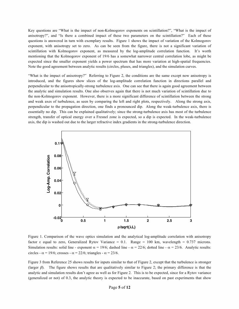
Key questions are “What is the impact of non-Kolmogorov exponents on scintillation?”, “What is the impact of anisotropy?”, and “Is there a combined impact of these two parameters on the scintillation?” Each of these questions is answered in turn with exemplary results. Figure 1 shows the impact of variation of the Kolmogorov exponent, with anisotropy set to zero. As can be seen from the figure, there is not a significant variation of scintillation with Kolmogorov exponent, as measured by the log-amplitude correlation function. It’s worth mentioning that the Kolmogorov exponent of 19/6 has a somewhat narrower central correlation lobe, as might be expected since the smaller exponent yields a power spectrum that has more variation at high-spatial frequencies. Note the good agreement between analytic results (circles, pluses, and triangles), and the simulation curves.

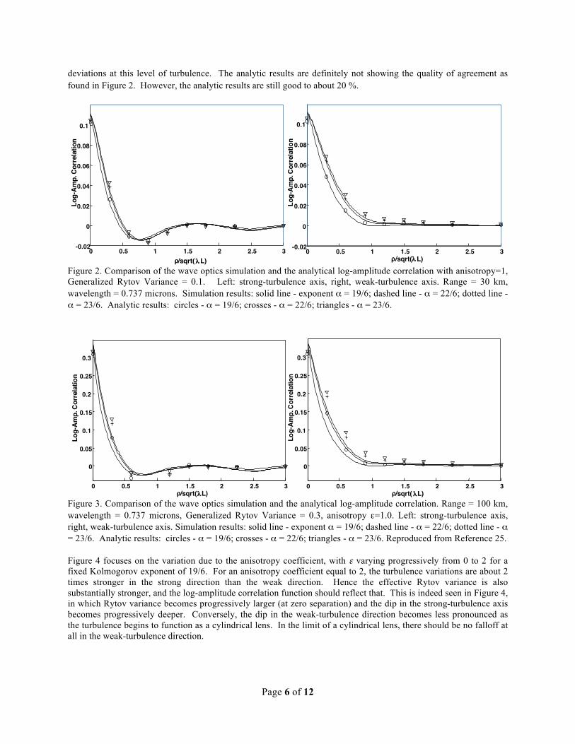
“What is the impact of anisotropy?” Referring to Figure 2, the conditions are the same except now anisotropy is introduced, and the figures show slices of the log-amplitude correlation function in directions parallel and perpendicular to the anisotropically-strong turbulence axis. One can see that there is again good agreement between the analytic and simulation results. One also observes again that there is not much variation of scintillation due to the non-Kolmogorov exponent. However, there is a more significant difference of scintillation between the strong and weak axes of turbulence, as seen by comparing the left and right plots, respectively. Along the strong axis, perpendicular to the propagation direction, one finds a pronounced dip. Along the weak-turbulence axis, there is essentially no dip. This can be explained qualitatively; since the strong-turbulence axis has most of the turbulence strength, transfer of optical energy over a Fresnel zone is expected, so a dip is expected. In the weak-turbulence axis, the dip is washed out due to the larger refractive index gradients in the strong-turbulence direction.

Figure 1. Comparison of the wave optics simulation and the analytical log-amplitude correlation with anisotropy factor ε equal to zero, Generalized Rytov Variance = 0.1. Range = 100 km, wavelength = 0.737 microns. Simulation results: solid line - exponent α = 19/6; dashed line - α = 22/6; dotted line - α = 23/6. Analytic results: circles - α = 19/6; crosses - α = 22/6; triangles - α = 23/6.

Figure 3 from Reference 25 shows results for inputs similar to that of Figure 2, except that the turbulence is stronger (larger β). The figure shows results that are qualitatively similar to Figure 2; the primary difference is that the analytic and simulation results don’t agree as well as for Figure 2. This is to be expected, since for a Rytov variance (generalized or not) of 0.3, the analytic theory is expected to be inaccurate, based on past experiments that show

0 0.5 1 1.5 2 2.5 3-0.02

0

0.02

0.04

0.06

0.08

0.1

ρ/sqrt(λL)

Log-

Am

p. C

orre

latio

n

Page 6 of 12      

deviations at this level of turbulence. The analytic results are definitely not showing the quality of agreement as found in Figure 2. However, the analytic results are still good to about 20 %.

Figure 2. Comparison of the wave optics simulation and the analytical log-amplitude correlation with anisotropy=1, Generalized Rytov Variance = 0.1. Left: strong-turbulence axis, right, weak-turbulence axis. Range = 30 km, wavelength = 0.737 microns. Simulation results: solid line - exponent α = 19/6; dashed line - α = 22/6; dotted line - α = 23/6. Analytic results: circles - α = 19/6; crosses - α = 22/6; triangles - α = 23/6.

Figure 3. Comparison of the wave optics simulation and the analytical log-amplitude correlation. Range = 100 km, wavelength = 0.737 microns, Generalized Rytov Variance = 0.3, anisotropy ε=1.0. Left: strong-turbulence axis, right, weak-turbulence axis. Simulation results: solid line - exponent α = 19/6; dashed line - α = 22/6; dotted line - α = 23/6. Analytic results: circles - α = 19/6; crosses - α = 22/6; triangles - α = 23/6. Reproduced from Reference 25. Figure 4 focuses on the variation due to the anisotropy coefficient, with ε varying progressively from 0 to 2 for a fixed Kolmogorov exponent of 19/6. For an anisotropy coefficient equal to 2, the turbulence variations are about 2 times stronger in the strong direction than the weak direction. Hence the effective Rytov variance is also substantially stronger, and the log-amplitude correlation function should reflect that. This is indeed seen in Figure 4, in which Rytov variance becomes progressively larger (at zero separation) and the dip in the strong-turbulence axis becomes progressively deeper. Conversely, the dip in the weak-turbulence direction becomes less pronounced as the turbulence begins to function as a cylindrical lens. In the limit of a cylindrical lens, there should be no falloff at all in the weak-turbulence direction.

0 0.5 1 1.5 2 2.5 3-0.02

0

0.02

0.04

0.06

0.08

0.1

ρ/sqrt(λL)

Log-

Am

p. C

orre

latio

n

0 0.5 1 1.5 2 2.5 3-0.02

0

0.02

0.04

0.06

0.08

0.1

ρ/sqrt(λL)

Log-

Am

p. C

orre

latio

n

0 0.5 1 1.5 2 2.5 3

0

0.05

0.1

0.15

0.2

0.25

0.3

ρ/sqrt(λL)

Log-

Am

p. C

orre

latio

n

0 0.5 1 1.5 2 2.5 3

0

0.05

0.1

0.15

0.2

0.25

0.3

ρ/sqrt( λL)

Log-

Am

p. C

orre

latio

n

Page 7 of 12      

 Figure 4. Comparison of the wave optics simulation and the analytical log-amplitude correlation. Range = 30 km, wavelength = 0.737 microns, Generalized Rytov Variance = 0.1, Kolmogorov exponent α = 19/6. Left: strong-turbulence axis, right, weak-turbulence axis. Simulation results: solid line - ε = 0; dashed line - ε = 1; dotted line - ε = 2. Analytic results: circles - ε = 0; crosses - ε = 1; triangles - ε = 2. The above section compares analytic results to simulations for paths with turbulence of uniform strength, and the comparison is good, especially for weaker turbulence, as is found at the AMOS Haleakala site.

5. SIMULATION APPLIED TO AMOS CONDITIONS

With the results from the previous section, the simulation can be applied to light received at AMOS from distant objects. Since the turbulence strength is non-uniform, the latter part of the analysis of Section 3 does not apply; however the simulation can accept non-uniform turbulence strength along the path. Hence the simulation is applied, using the widely-accepted Maui-3 turbulence model. The Maui-3 turbulence model is based on measurements that likely assume Kolmogorov turbulence to estimate the refractive-index structure function Cn

2 as a function of altitude h, from raw measurements. To apply the simulation correctly to non-Kolmogorov turbulence, the structure function should thus be adapted based on both the Kolmogorov exponent and the anisotropy. This could be done, but if the underlying measurements were not from Kolmogorov turbulence in the first place, the form of this adaptation is not clear. Hence, for simplicity, the numerical values of the Maui-3 model are used for all cases shown in this section, for the turbulence strength, to show parametric trends.

The simulation uses the same settings as above for the propagation grids. In particular the grids are 1024 x 1024 in size and the grid point spacing is set to 5 mm. Smaller grid point spacings were simulated; no significant changes in the results were observed. Light at 800 nm is propagated from a distant space-based source with an altitude of 250 km and a zenith angle of 40 degrees. 10 phase screens were used for the propagation, with non-uniform spacing in the first 25 km of the atmosphere. The simulation results were compared against the known Rytov variance for the Kolmogorov case, and matched to within a few percent for a variety of zenith angles.

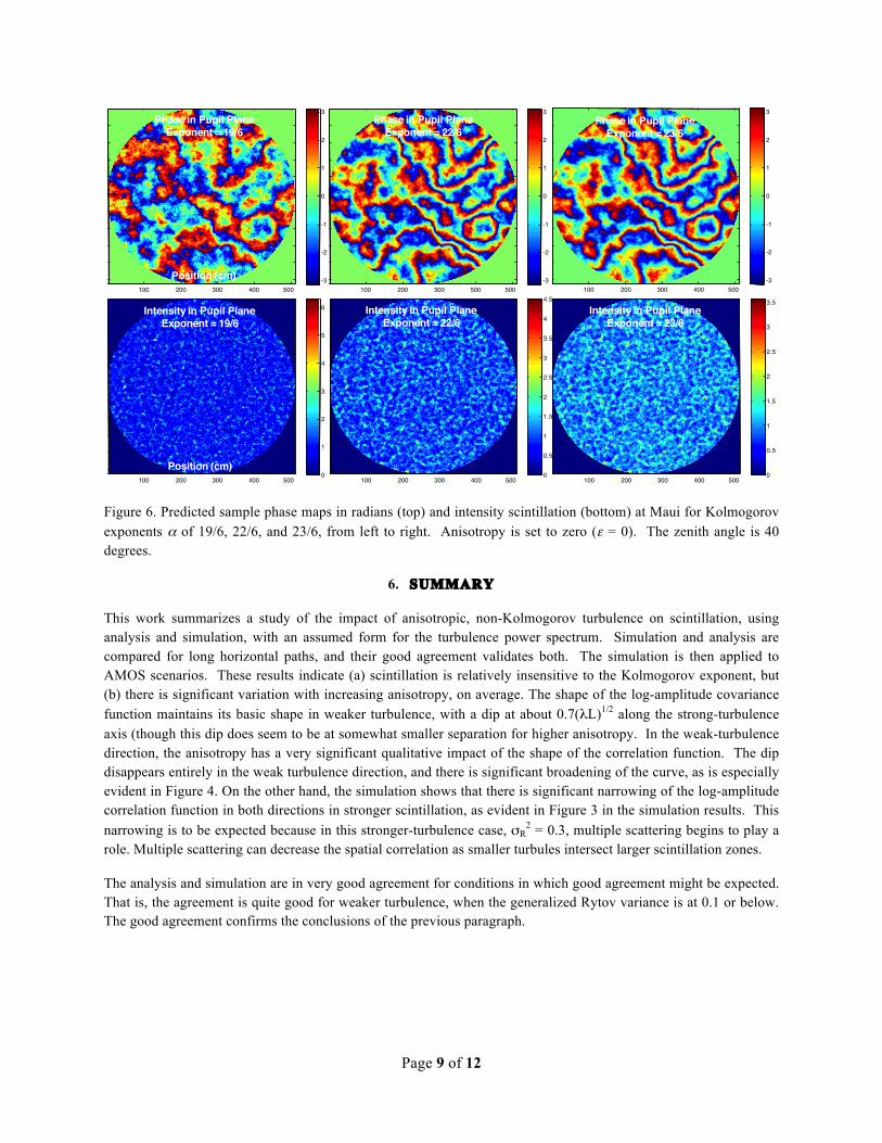
Figure 5 shows sample phase maps and sample scintillation (intensity) in the pupil for three different anisotropies, with the usual Kolmogorov exponent (22/6), at a zenith angle of 40 degrees. Figure 6 shows the same sample phase maps and sample scintillation for three different Kolmogorov exponents, 19/6, 22/6, and 23/6, but no anisotropy. Figure 5 clearly shows the impact of anisotropy on both the phase and the intensity scintillation. In Figure 6, the impact of Kolmogorov exponent is more subtle, but nonetheless discernible. For example, it can be seen that for an exponent of 19/6, the higher frequencies of the phase are more noticeable, and the scintillation is significantly stronger.

0 0.5 1 1.5 2 2.5 3

0

0.05

0.1

0.15

0.2

ρ /sqrt(λL)

Log-

Am

p. C

orre

latio

n

0 0.5 1 1.5 2 2.5 3

0

0.05

0.1

0.15

0.2

ρ /sqrt(λL)

Log-

Am

p. C

orre

latio

n

Page 8 of 12      

Figure 5. Predicted sample phase maps in radians (top) and intensity scintillation (bottom) at Maui for anisotropies of ε = 0, 1, and 2, from left to right. Kolmogorov exponent is set 22/6, (standard Kolmogorov turbulence). The zenith angle of the source is 40 degrees.

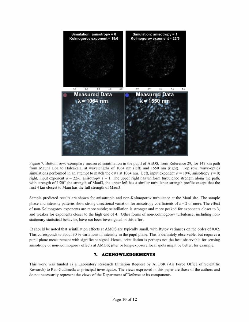
Figure 7 shows measured data from reference 29, Figure 7, along with simulated results. The bottom row shows exemplary measured data at 1064 nm on the left, and for 1550 nm on the right, for propagation over a path of 149 km between Mauna Loa and Haleakala. A number of simulations were performed to match the data at 1064 nm. The top row shows two simulations at 1064 nm that were the best of many matches in terms of qualitative appearance. The upper left figure shows a sample simulation case with a Kolmogorov exponent α of 19/6, and zero anisotropy. The turbulence strength was roughly equal to that of the Maui 3 model in the first 4 km, and then was about 1/20th of the Maui 3 model, in order to account for the increased elevation of the path above the earth’s surface. This upper left case has a scintillation index of about 2.0, and shows the salt-and-pepper high-frequency scintillation that matches the exemplary data in the lower left. The upper right portion of Figure 7 shows a sample simulation case with the standard Kolmogorov exponent of 22/6, and an anisotropy ε of 1. In this case, larger voids and scintillation structures are apparent than in the measured data. Furthermore, a distinctive anisotropy is apparent in the simulation, somewhat more than in the measured data. In this case, the scintillation index is about 2.2; the lower-strength turbulence (1/20th) is used over the entire path to avoid an excessive scintillation index of 3 or more in this case. In all cases, the simulation uses 1024 x 1024 grids, 5 mm grid-point spacing, and 60 phase screens, as described above. Based on these and other related runs, it is believed that the turbulence power spectrum is closer to -1, as discussed in reference 29, and that not much anisotropy is present on the path. Further, a strong turbulence layer is likely in the first 2-4 kilometers of the path nearest Maui. This conclusion has a least one caveat – that the measurements were taken at an image of the pupil. If the pupil is not precisely imaged, there will be amplification of small-scale scintillation which was not included in the simulation.

Phase in Pupil PlaneAnisotropy ε = 0

100 200 300 400 500-3

-2

-1

0

1

2

3Phase in Pupil Plane

Anisotropy ε = 1

100 200 300 400 500-3

-2

-1

0

1

2

3Phase in Pupil Plane

Anisotropy ε = 2

100 200 300 400 500-3

-2

-1

0

1

2

3

Intensity in Pupil PlaneAnisotropy ε = 0

100 200 300 400 5000

0.5

1

1.5

2

2.5

3

3.5

4

4.5

Intensity in Pupil PlaneAnisotropy ε = 1

100 200 300 400 5000

0.5

1

1.5

2

2.5

3

3.5

4Intensity in Pupil Plane

Anisotropy ε = 2

100 200 300 400 5000

0.5

1

1.5

2

2.5

3

3.5

4

Position (cm)

Position (cm)

Page 9 of 12      

Figure 6. Predicted sample phase maps in radians (top) and intensity scintillation (bottom) at Maui for Kolmogorov exponents α of 19/6, 22/6, and 23/6, from left to right. Anisotropy is set to zero (ε = 0). The zenith angle is 40 degrees.

6. SUMMARY

This work summarizes a study of the impact of anisotropic, non-Kolmogorov turbulence on scintillation, using analysis and simulation, with an assumed form for the turbulence power spectrum. Simulation and analysis are compared for long horizontal paths, and their good agreement validates both. The simulation is then applied to AMOS scenarios. These results indicate (a) scintillation is relatively insensitive to the Kolmogorov exponent, but (b) there is significant variation with increasing anisotropy, on average. The shape of the log-amplitude covariance function maintains its basic shape in weaker turbulence, with a dip at about 0.7(λL)1/2 along the strong-turbulence axis (though this dip does seem to be at somewhat smaller separation for higher anisotropy. In the weak-turbulence direction, the anisotropy has a very significant qualitative impact of the shape of the correlation function. The dip disappears entirely in the weak turbulence direction, and there is significant broadening of the curve, as is especially evident in Figure 4. On the other hand, the simulation shows that there is significant narrowing of the log-amplitude correlation function in both directions in stronger scintillation, as evident in Figure 3 in the simulation results. This narrowing is to be expected because in this stronger-turbulence case, σR

2 = 0.3, multiple scattering begins to play a role. Multiple scattering can decrease the spatial correlation as smaller turbules intersect larger scintillation zones.

The analysis and simulation are in very good agreement for conditions in which good agreement might be expected. That is, the agreement is quite good for weaker turbulence, when the generalized Rytov variance is at 0.1 or below. The good agreement confirms the conclusions of the previous paragraph.

Intensity in Pupil PlaneExponent = 22/6

100 200 300 400 5000

0.5

1

1.5

2

2.5

3

3.5

4

4.5

Phase in Pupil PlaneExponent = 19/6

100 200 300 400 500-3

-2

-1

0

1

2

3

100 200 300 500 500-3

-2

-1

0

1

2

3Phase in Pupil Plane

Exponent = 22/6

100 200 300 400 500-3

-2

-1

0

1

2

3Phase in Pupil Plane

Exponent = 23/6

100 200 300 400 5000

1

2

3

4

5

6Intensity in Pupil PlaneExponent = 19/6

100 200 300 400 5000

0.5

1

1.5

2

2.5

3

3.5Intensity in Pupil Plane

Exponent = 23/6

Position (cm)

Position (cm)

Page 10 of 12    

Figure 7. Bottom row: exemplary measured scintillation in the pupil of AEOS, from Reference 29, for 149 km path from Mauna Loa to Haleakala, at wavelengths of 1064 nm (left) and 1550 nm (right). Top row, wave-optics simulations performed in an attempt to match the data at 1064 nm. Left, input exponent α = 19/6, anisotropy ε = 0; right, input exponent α = 22/6, anisotropy ε = 1. The upper right has uniform turbulence strength along the path, with strength of 1/20th the strength of Maui3, the upper left has a similar turbulence strength profile except that the first 4 km closest to Maui has the full strength of Maui3. Sample predicted results are shown for anisotropic and non-Kolmogorov turbulence at the Maui site. The sample phase and intensity patterns show strong directional variation for anisotropy coefficients of ε = 2 or more. The effect of non-Kolmogorov exponents are more subtle; scintillation is stronger and more peaked for exponents closer to 3, and weaker for exponents closer to the high end of 4. Other forms of non-Kolmogorov turbulence, including non-stationary statistical behavior, have not been investigated in this effort.

It should be noted that scintillation effects at AMOS are typically small, with Rytov variances on the order of 0.02. This corresponds to about 30 % variations in intensity in the pupil plane. This is definitely observable, but requires a pupil plane measurement with significant signal. Hence, scintillation is perhaps not the best observable for sensing anisotropy or non-Kolmogorov effects at AMOS; jitter or long-exposure focal spots might be better, for example.

7. ACKNOWLEDGEMENTS

This work was funded as a Laboratory Research Initiation Request by AFOSR (Air Force Office of Scientific Research) to Rao Gudimetla as principal investigator. The views expressed in this paper are those of the authors and do not necessarily represent the views of the Department of Defense or its components.

Measured Dataλ = 1064 nm

Measured Dataλ = 1550 nm

1.0 2.0 3.0 4.0 5.0

Simulation: anisotropy = 0Kolmogorov exponent = 19/6

1.0 2.0 3.0 4.0 5.0

Simulation: anisotropy = 1Kolmogorov exponent = 22/6

Page 11 of 12    

8. REFERENCES

1. Mikhail S. Belen’kii, Edward Cuellar, Kevin A. Hughes, and Vincent A. Rye, “Experimental Study of Spatial Structure of Turbulence at Maui Space Surveillance Site (MSSS),” Proc. SPIE 6304, 63040U, 2006.

2. M. S. Belen’kii, J. D. Barchers, S. J. Karis, C. L. Osmon, J. M. Brown II, and R. Q. Fugate, “Preliminary experimental evidence of anisotropy of turbulence and the effect of non-Kolmogorov turbulence on wavefront tilt statistics,” Proc. SPIE 3762, 396–406, 1999.

3. M. S. Be1en’kii, S. J. Karis, J. M. Brown, and R. Q. Fugate, “Experimental evidence of the effects of non-Kolmogorov turbulence and anisotropy of turbulence,” Proc. SPIE 3749, 50-51, 1999.

4. M. S. Be1en’kii, S. J. Karis, J.M. Brown, and R. Q. Fugate, “Experimental study of the effect of non-Kolmogorov stratospheric turbulence on star image motion,” Proc. SPIE 3126, 113-123, 1997.

5. M. Vorontsov, G. W. Carhart, V. S. Rao Gudimetla, T. Weyrauch, E. Stevenson, S. L. Lachinova, L. A. Beresnev, J. Liu , K. Rehder and J. F Riker, “ Characterization of atmospheric turbulence effects over 149 km propagation path using multi-wavelength laser beacons,” Proc. AMOS Technologies Conference, P. Kervan, ed., (Amostech, 2011, Maui, Hawaii).

6. A. Consortini, L. Ronchi and L. Stefanutti, “Investigation of Atmospheric Turbulence by Narrow Laser beams, “ Appl. Opt. 9, pp. 2543-2547, 1970.

7. R. M. Manning, “An Anisotropic Turbulence Model for Wave Propagation near the Surface of the Earth,” IEEE Trans. on Antennas and Propagation, AP-34, pp. 258-262, 1986.

8. A. Silverman, E. Golbraikh, and N. S. Kopeika, “Lidar studies of aerosols and non-Kolmogorov turbulence in the Mediterranean troposphere,” Proc. SPIE 5987, 598702-1-12, 2005.

9. D. T. Kyrazis, J. Wissler, D. B. Keating, A. J. Preble, and K. P. Bishop, “Measurement of optical turbulence in the upper troposphere and lower stratosphere,” Proc. SPIE 2110, 43-55, 1994.

10. A. P. Aleksandrov, G. M. Grechko, A. S. Gurvich, V. Kan, M. K. H. Manarov, A. I. Pokhomov, Yu. V., Romanenko, S. A. Savchenko, S. I. Serova and Y. G. Titov, “Spectra of Temperature Variations in the Stratosphere as indicated by Satellite-borne Observation of the Twinkling of Stars, “ Izvestiya, Atmospheric and Oceanic Physics, 26, pp. 5-16, 1990.

11. Clélia Robert, Jean-Marc Conan, Vincent Michau, Jean-Baptiste Renard, Claude Robert, and Francis Dalaudier, "Retrieving parameters of the anisotropic refractive index fluctuations spectrum in the stratosphere from balloon-borne observations of stellar scintillation," J. Opt. Soc. Am. A 25, 379-393, 2008.

12. A. S. Gurvich and M. S. Belen'kii, "Influence of stratospheric turbulence on infrared imaging," J. Opt. Soc. Am. A 12, 2517-2522, 1995.

13. A. P. Aleksandrov, G. M. Grechko, A. S. Gurvich, V. Kan, M. K. H. Manarov, A. I. Pokhomov, Yu. V., Romanenko, S. A. Savchenko, S. I. Serova and Y. G. Titov, “Spectra of Temperature Variations in the Stratosphere as indicated by Satellite-borne Observation of the Twinkling of Stars, “ Izvestiya, Atmospheric and Oceanic Physics, 26, pp. 5-16, 1990.

14. L.V. Antoshkin, N.N. Botygina, O.N. Emaleev. L.N. Lavrinova, V.P. Lukin, A.P. Rostov, B.V. Fortes, and A.P. Yankov, “Investigation of Turbulence Spectrum Anisotropy in the Ground Atmospheric Layer; Preliminary Results,” Atmos. Oceanic. Opt. 8, pp. 993-996, 1995.

15. V. E. Ostashev and D. K. Wilson, “Log-amplitude and phase fluctuations of a plane wave propagating through anisotropic, inhomogeneous turbulence,” Acustica-acta Acustica, 87, pp.685-694, 2001.

16. V. E. Ostashev, D. K. Wilson and G. H. Goedecke, “Spherical Wave Propagation through Inhomogeneous, Anisotropic Turbulence: Log-amplitude and Phase Correlations, “J. Acoust. Soc. Am., 115(1), pp. 120-130, 2004.

17. D. L. Fried and J. D. Cloud, “Propagation of an Infinite Plane Wave in a Randomly Inhomogeneous Medium,” J. Opt. Soc. Am. 56, pp. 1667-1676, 1966.

18. S. F. Clifford, “The Classical Theory of Wave Propagation in a Turbulent Medium,” in Laser Beam Propagation in the Atmosphere, J. W. Strohbehn, ed., (Springer-Verlag, New York, 1978).

Page 12 of 12    

19. Richard J. Sasiela, “Electromagnetic Wave Propagation in Turbulence,” (Springer-Verlag, New York, 1994).

20. Albert D. Wheelon, “Electromagnetic Scintillation, Vol. 2 (Weak scattering),” Chapter 3 (Cambridge University Press, Cambridge, 2001).

21. Larry C. Andrews and R. L. Phillips, “Laser beam Propagation in Random Media,” (SPIE Press, Bellingham, Washington, 2005).

22. Italo Toselli, Brij Agrawal, and Sergio Restaino, "Light propagation through anisotropic turbulence," J. Opt. Soc. Am. A 28, 483-488, 2011.

23. B. E. Stribling, B. M. Welsh, and M. C. Roggemann, “Optical propagation in non-Kolmogorov atmospheric turbulence,” Proc. SPIE 2471, 181-196, 1995.

24. V. S. Rao Gudimetla, Richard B. Holmes, Carey Smith, and Gregory Needham, “Analytical expressions for the log-amplitude correlation function of a plane wave through anisotropic atmospheric refractive turbulence,” J. Opt. Soc. Am. A, Vol. 29, pp. 832-841, 2012.

25. V. S. Rao Gudimetla, Richard B. Holmes, Jim Riker, “Analytical expressions for the log-amplitude correlation function for plane wave through anisotropic non-Kolmogorov refractive turbulence,” J. Opt. Soc. Am. A, Vol. 29, pp. 2622-2627, 2012.

26. J. M. Martin and Stanley M. Flatté, "Intensity images and statistics from numerical simulation of wave propagation in 3-D random media," Appl. Opt. 27, 2111-2126, 1988.

27. J. M. Martin and Stanley M. Flatté, "Simulation of point-source scintillation through three-dimensional random media," J. Opt. Soc. Am. A 7, 838-847, 1990

28. Jason D. Schmidt, “Numerical Simulation of Optical Wave Propagation with Examples in MATLAB”, (SPIE Press, Bellingham, Washington, 2010).

29. M. Vorontsov, V. S. Rao Gudimetla, G. Carhart, T. Weyrauch, S. Lachinova, J. Reierson, L. Beresnev, J. Liu, J. F Riker, “Comparison of turbulence-induced scintillations for multi-wavelength laser beacons over tactical (7 km) and long (149 km) atmospheric propagation paths” Proc. AMOS Technologies Conference, P. Kervan, ed., (Amostech, Maui, Hawaii, , 2011).