schubert calculus and quiver varietiespzinn/icr/knutson.pdf · an intersection theory problem. let...

Schubert calculus and quiver varieties

Allen Knutson (Cornell)

Integrability, Combinatorics, and Representations, 2019

AbstractSchubert calculus, the intersection theory of homogeneous spaces such

as Grassmannians (or “1-step flag manifolds”), is famously a problem forwhich we have easy alternating-sum formulæ but know in advance thatthe intersection numbers will be nonnegative. We’ve had positive rules(i.e. counting a set, such as Young tableaux) for the Grassmannian casesince 1934, but 2-step and 3-step rules only came in 2009 and 2017.

I’ll explain how connecting these “puzzle” rules to quantum integrablesystems made them easy to derive and prove, and how further connectionto quiver varieties has brought about several more advances. This work isjoint with Paul Zinn-Justin and Iva Halacheva (both of Melbourne).

These transparencies are available at http://math.cornell.edu/∼allenk/

An intersection theory problem.

Let L1, L2 be two different, but crossing, lines in 3-space.Let Y1, Y2 be the set of lines touching L1, L2 respectively. Then

Y1 ∩ Y2 = {lines in the L1L2 plane}⋃

{lines doing both}

{lines through L1 ∩ L2}

Let Gr(1,P3) ∼= Gr(2,C4) be the Grassmannian of lines in projective 3-space.Although Y1 6= Y2 as sets, they are homologous in Gr(2,C4), so define the sameelement “S0101” in cohomology (or K-theory).

More generally, consider lines in Pn−1 that touch a fixed j-plane and are

contained in a fixed k-plane. Make a length n binary string λ with two zeros, inpositions n− k, n− j, and let Sλ denote the cohomology (or K-theory) class.

Then the above lets us compute

(S0101)2 = S1001+S0110 in H∗(Gr(2,C4))

(

or that minus S1010, in K(Gr(2,C4)))

These transparencies are available at http://math.cornell.edu/∼allenk/ 1

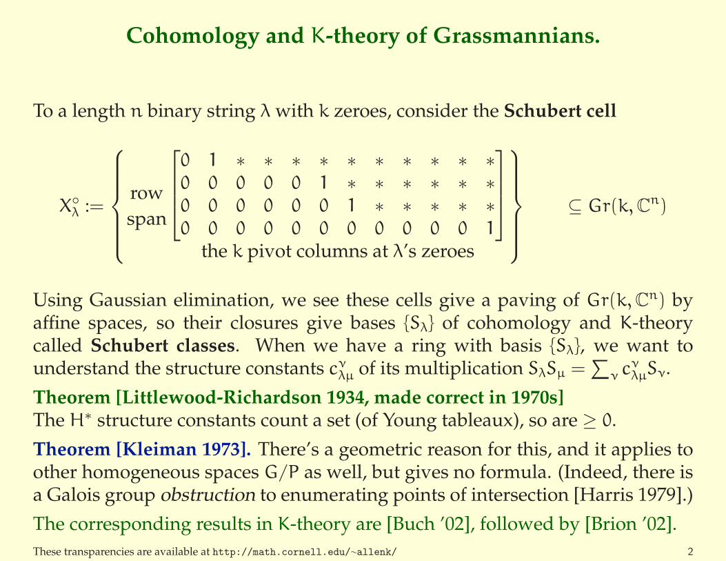
Cohomology and K-theory of Grassmannians.

To a length n binary string λ with k zeroes, consider the Schubert cell

X◦λ :=

row

span

0 1 ∗ ∗ ∗ ∗ ∗ ∗ ∗ ∗ ∗ ∗0 0 0 0 0 1 ∗ ∗ ∗ ∗ ∗ ∗0 0 0 0 0 0 1 ∗ ∗ ∗ ∗ ∗0 0 0 0 0 0 0 0 0 0 0 1

the k pivot columns at λ’s zeroes

⊆ Gr(k,Cn)

Using Gaussian elimination, we see these cells give a paving of Gr(k,Cn) byaffine spaces, so their closures give bases {Sλ} of cohomology and K-theorycalled Schubert classes. When we have a ring with basis {Sλ}, we want tounderstand the structure constants cνλµ of its multiplication SλSµ =

∑ν c

νλµSν.

Theorem [Littlewood-Richardson 1934, made correct in 1970s]The H∗ structure constants count a set (of Young tableaux), so are ≥ 0.

Theorem [Kleiman 1973]. There’s a geometric reason for this, and it applies toother homogeneous spaces G/P as well, but gives no formula. (Indeed, there isa Galois group obstruction to enumerating points of intersection [Harris 1979].)

The corresponding results in K-theory are [Buch ’02], followed by [Brion ’02].


A first formula for the structure constants of H∗T(Gr(k,Cn)).

Theorem [K-Tao, ’03]. Glue these puzzle pieces(which may be rotated) into puzzles, whicharen’t permitted 10-labels on the boundary.

Then in H∗, cνλµ is the number of puzzleswith boundary conditions λ, µ, ν like so:

0 0

0

1 1

1

1 0

10

λ µν

In fact our result is in torus-equivariant cohomology, with structure constantscνλµ now in H∗

T(pt)∼= Z[y1, . . . , yn]:

0

1

0

1

1

0

1

010

11

00

11

1 11

1 1

10

100 10

00

0000

0

1

0

1

1

0

1

010

11

00

00

00 0

110

111

1

0 0

1 1 10 0

1

0

1

1

0

1

010

11

00

00

111

0 0

0 11

1

0 0

110 10

(S0101)2 = S1001 + S0110 + (y2 − y3)S0101

The equivariant piece doesn’t break into triangles, can’t be rotated, andcontributes a factor of yi − yj according to its position.These transparencies are available at http://math.cornell.edu/∼allenk/ 3

Puzzles for multistep flag manifolds.

A d-step flag manifold Fl(n1, n2, . . . , nd; Cn) is the space of chains

{0 ≤ Vn1 ≤ Vn2 ≤ . . . ≤ Vnd ≤ Cn} of subspaces with a fixed list of

dimensions, the d = 1 case being Grassmannians. This manifold too comeswith a decomposition into Schubert cells, now indexed by strings in {0, 1, . . . , d}

with multiplicities given by the differences ni+1 − ni (where n0 = 0, nd+1 = n).

Conjecture [K 1999], Theorem [Buch-Kresch-Purbhoo-Tamvakis ’16].The same puzzle count computes structureconstants in H∗(Fl(n1, n2; C

n)), requiringonly these new puzzle pieces (& rotations):

2 0

20

2 1

21

2 10

2(10)

2 2

2

21 0

(21)0

Their lengthy and delicate proof is that my puzzle rule is associative. It’srelatively easy to check that it gives the correct multiplication by generators.

So, apparently one wants numbers 0, 1, 2 around the outside of the puzzle pluson the inside, “multinumbers” (XY) where all X > all Y. I found that theanalogous 3-step multinumbers gave 23 labels and didn’t quite work.

Corrected conjecture [Buch ’06], Theorem [K–Zinn-Justin].The same puzzle count computes d = 3 structure constants, but one needs 27

labels, the ones I missed being (3(21))(10), (32)((21)0), 3(((32)1)0), (3(2(10)))0.


Example. A 2-step puzzle in which all 8 labels appear.

1

0 0

1 1

2(10)

2 10

0

210 1

21

0

21

21

0

1

0

10

1

0

1

11

1

1

10 1

0

00

0

2

2 20 2

0

0

0

20

0

2

(21)0


A dual picture: scattering diagrams and a surprise.

The n triangles on the bottom of a puzzle shapeare different from the others: they can’t occurin an equivariant piece. Let’s pair up the othertriangles into vertical rhombi.Now, let’s look at the graph-theory dual of anequivariant puzzle, an overlay of n Ys.

This one is worth (y1 − y2)(y2 − y4):

1 1

0

11

0

0

0

0

01

10

1

01

0

1

1 0

10

1

0 0

1 0

If V is the 3-d space with basis ~0,~1, ~10, then we can regard the options at acrossing as giving a matrix R : V⊗V → V⊗V ; at a trivalent vertex as a matrixU : V⊗V → V∗; and the puzzle formula as a matrix coefficient V⊗2n → (V∗)⊗n.

That’s not quite right because of the yi − yj coefficients; we need the tensorfactors V to “carry” these parameters in some sense, (V, yi).

Observation [Zinn-Justin ’05].Rotating the nonrotatable equivariant piecesappropriately (!?), the equivariant puzzleR-matrix satisfies the Yang-Baxter equation:

(V,a) (V,b) (V,c)

(V,a)(V,b)(V,c)

(V,a) (V,b) (V,c)

(V,a)(V,b)(V,c)


YBE and bootstrap proof that puzzles compute cνλµ ∈ H∗T .

Enough to check restrictions to fixed points: [Xλ]|σ [Xµ]|σ =∑

ν cνλµ[Xν]|σ.

Theorem [K-ZJ ’17 ?].1. With any choice of orientations, colors, and boundary conditions, we havethe first two equations on scattering amplitudes, implying the third:

2. If a puzzle has the identity on the bottom, it must also have it on the NW andNE sides, and have scattering amplitude = 1.

Hence

λ µ

σ

sort( ) λ

sort( ) λ

sort( ) λ sort( ) λ

σ σ

λ µ

σ σ

λ µ

so there’s our [Xλ]|σ [Xµ]|σ. Of course proposition #1 above is a big case check.


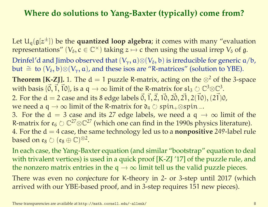
Where do solutions to Yang-Baxter (typically) come from?

Let Uq(g[z±]) be the quantized loop algebra; it comes with many “evaluation

representations” (Vδ, c ∈ C×) taking z 7→ c then using the usual irrep Vδ of g.

Drinfel ′d and Jimbo observed that (Vγ, a)⊗(Vδ, b) is irreducible for generic a/b,but ∼= to (Vδ, b)⊗(Vγ, a), and these isos are “R-matrices” (solution to YBE).

Theorem [K-ZJ]. 1. The d = 1 puzzle R-matrix, acting on the ⊗2 of the 3-space

with basis {~0,~1,~10}, is a q→∞ limit of the R-matrix for sl3 � C3⊗C

3.

2. For the d = 2 case and its 8 edge labels ~0,~1,~2, ~10, ~20, ~21, ~2(10), ~(21)0,we need a q→∞ limit of the R-matrix for d4 � spin+⊗spin−.3. For the d = 3 case and its 27 edge labels, we need a q → ∞ limit of theR-matrix for e6 � C

27⊗C27 (which one can find in the 1990s physics literature).

4. For the d = 4 case, the same technology led us to a nonpositive 249-label rulebased on e8 � (e8 ⊕ C)⊗2.

In each case, the Yang-Baxter equation (and similar “bootstrap” equation to dealwith trivalent vertices) is used in a quick proof [K-ZJ ’17] of the puzzle rule, andthe nonzero matrix entries in the q→∞ limit tell us the valid puzzle pieces.

There was even no conjecture for K-theory in 2- or 3-step until 2017 (whicharrived with our YBE-based proof, and in 3-step requires 151 new pieces).


Revisiting associativity at d = 1.

The sl3-equivariant map C3⊗C

3 → Alt2C3 only allowsfermionic mixing, i.e. of different basis vectors, whichis not what we saw in the first two pieces:

0 0

0

1 1

1

1 0

10

Reformulation of the Grassmannian puzzle rule. Consider the puzzle pieces

ba ab

a^b

a^bwhere a, b ∈ {0, 1, 2}, a 6= b, and excluding a = 0, b = 2 forsome weird reason. Then we can compute cνλµ using puzzleswith µ on the Northeast, λ on the Northwest but written in 1sand 2s, and ν on the South but written in 0∧ 1s and 1∧ 2s.

Associativity says that the coefficients of So in(SλSµ)Sν and Sλ(SµSν) are the same. In puzzleterms, we label the front or back of a tetrahedronwith bipuzzles, and should be able to biject them:

λ µ

ο ν ν

µλ

ο= ##

Theorem [Henriques ∼’04]. One can compute coλµν using any lattice surface Σ

in the tetrahedron with ∂Σ this same (λ, µ, ν, o) boundary.Proof: ∃ 3-d puzzle pieces giving correspondences between Σ- and Σ ′-puzzles.

[Halacheva-Perry-ZJ] All is much simpler and extends to K-theory if ν iswritten in 0s and 1s, while µ is written in 1s and 2s, and λ in 2s and 3s.


Example. Before and after reformulation.

0

1

0

1

1 0

1

1

1

0

1010

1010

0

11

11

11 1

11

111 10

1

110 0

10

00

0 0 0011

10 10 1

2

1

2

2 0

1

1

1

0

2020

20 21

21 21

21 21

21 21 21

212010

10

10 10

212

12121012

1 0 1 2 1


Nakajima’s geometry of some Uq(g[z±]) representations.

But why should such representations come up in studying Fl(n1, n2, . . . , nd; Cn)?

Given an oriented graph (Q0, Q1), with some vertices declared “gauged” andthe others “framed”, double it by adding a backwards arrow for every arrow.Attach a vector space Wi to each framed vertex and Vj to each gauged vertex.

Definition. A point in the quiver variety M(Q0, Q1,W, V) is a choice of lineartransformation for every edge,

• such that∑

± (go out) ◦ (come back in) is zero at each gauged vertex;• every ~v in each Vi can leak into some Wj via some path;• all is considered up to

∏iGL(Vi) change-of-bases at the gauged vertices.

Let M(Q0, Q1,W) :=∐

W M(Q0, Q1,W, V) be the quiver scheme.

Theorem [Nakajima ’01]. If Q is ADE, then Uq(its g[z±]) � K(M(Q0, Q1,W)).

Main example. M

n↑nd ← nd−1 ← . . .← n1

∼= T∗Fl(n1, . . . , nd; C

n).

For this framing the Uq(sld+1[z±])-action appears already in [Ginzburg-

Vasserot 1993], and the rep is K(M(Q0, Q1, nω1)) ∼= (Cd+1)⊗n, whose weightmultiplicities are (d+ 1)-nomial coefficients.


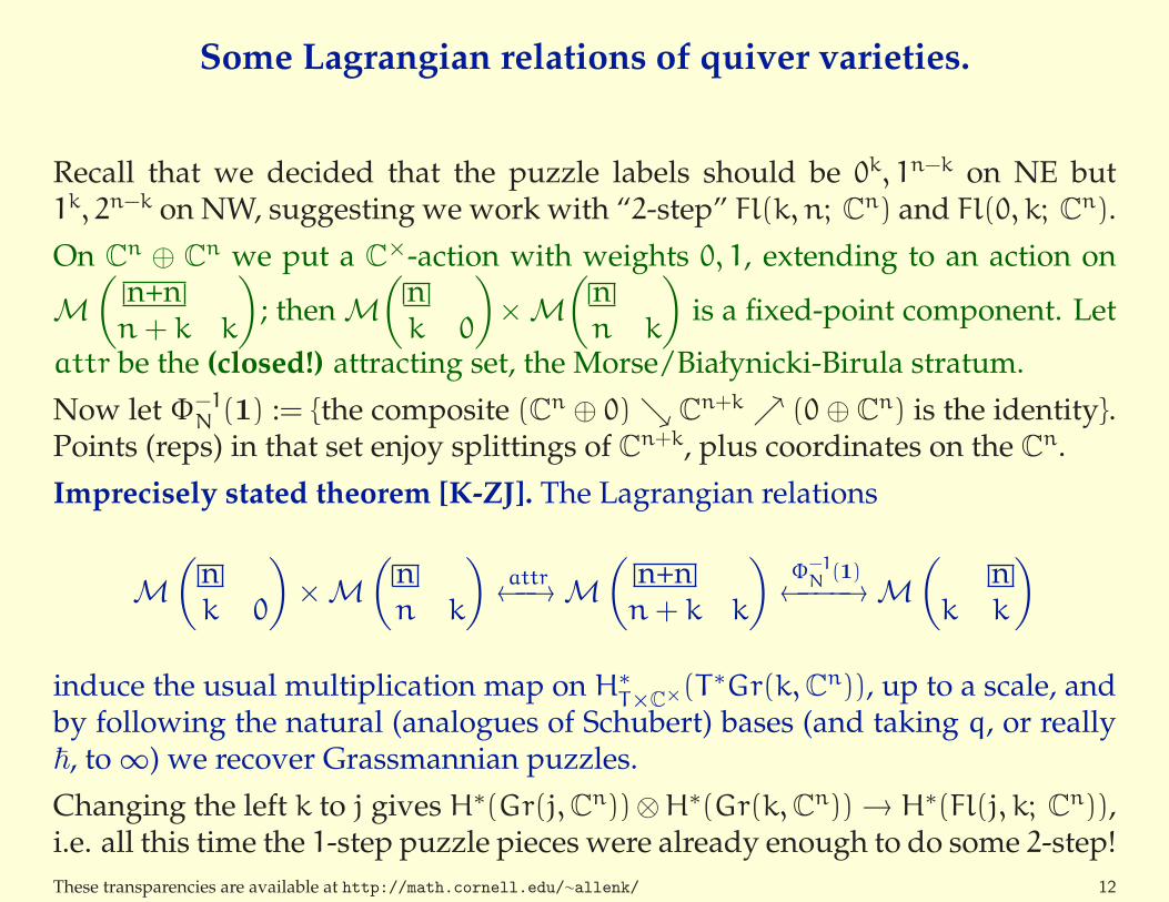
Some Lagrangian relations of quiver varieties.

Recall that we decided that the puzzle labels should be 0k, 1n−k on NE but1k, 2n−k on NW, suggesting we work with “2-step” Fl(k, n; Cn) and Fl(0, k; Cn).

On Cn ⊕ C

n we put a C×-action with weights 0, 1, extending to an action on

M

(

n+nn+ k k

)

; then M

(

nk 0

)

×M

(

nn k

)

is a fixed-point component. Let

attr be the (closed!) attracting set, the Morse/Białynicki-Birula stratum.

Now let Φ−1N (1) := {the composite (Cn ⊕ 0)ց C

n+k ր (0⊕ Cn) is the identity}.

Points (reps) in that set enjoy splittings of Cn+k, plus coordinates on the Cn.

Imprecisely stated theorem [K-ZJ]. The Lagrangian relations

M

(

nk 0

)

×M

(

nn k

)

attr←−→M

(

n+nn+ k k

)

Φ−1N

(1)←−−−→M

(

nk k

)

induce the usual multiplication map on H∗T×C×(T

∗Gr(k,Cn)), up to a scale, andby following the natural (analogues of Schubert) bases (and taking q, or really~, to∞) we recover Grassmannian puzzles.

Changing the left k to j gives H∗(Gr(j,Cn))⊗H∗(Gr(k,Cn))→ H∗(Fl(j, k; Cn)),i.e. all this time the 1-step puzzle pieces were already enough to do some 2-step!


The newest Schubert calculus: separated descents.

Theorem [K-ZJ]. Consider the puzzle pieces at right, andtheir 180◦ rotations. Make size n puzzles with 1, . . . , k

and n−k blanks on NE side, k+1, . . . , n and k blanks onNW side. Then these compute the structure constants ofH∗(Fl(k, . . . , n;Cn)) ⊗ H∗(Fl(1, . . . , k;Cn))→ H∗(Fl(Cn)),and with two more pieces we get the KT -version.

i j

i>j

i i

[Kogan ’01], the previous state-of-the-art for general H∗(Fl(Cn)) calculations(extended to K-theory in [K-Yong ’04]), assumed that one of the two factorswas a Grassmannian (and was algorithmic, and nonequivariant).

“Proof”. Same recipe as last slide, using the Lagrangian relations

M

(

nn n . . . n k k− 1 . . . 1

)

×M

(

nn− 1 n− 2 . . . k 0 0 . . . 0

)

attr←−→M

(

n+n2n− 1 2n− 2 . . . n+ k k k− 1 . . . 1

)

Φ−1N

(1)←−−−→M

(

nn− 1 2n− 2 . . . n+ k k k− 1 . . . 1

)

∼= T∗Fl(Cn)


Example. A separated-descents puzzle.

4

6

7

5

1

3

2

5

5

51

51

7

7

7

7

1 5

5

53

53

1

176

53

16

6

4

6

6

7

7

7

1

5

5

4

4

6

6

31

7

7

7

1 3

1

1

3

3

5

5 2


Beyond quiver varieties and R-matrices.

The original puzzle rule based on these threepieces enjoys Grassmannian duality: flip a puzzleleft-right while exchanging 0s and 1s, comparingcomputations on Gr(k,Cn) and on Gr(n− k,Cn).

0 0

0

1 1

1

1 0

10

This prompts the question: what are self-dual puzzles good for?It turns out there are almost none of them, unless we allow equivariant piecesdown the centerline, so we build that into the definition of “self-dual puzzle”.

Theorem [Halacheva-K-ZJ]. Let J be an antidiagonal symplectic form on C2n,

and SpGr(k,C2n) :={V ∈ Gr(k,C2n) : V ≤ V⊥

}the symplectic Grassmannian.

Index its 2k(

nk

)

Schubert classes by strings µ of length n in 0, 1, 10 with n−k 10s.

Then the restriction ι∗(Sλ) =∑

µ dµλ Sµ of a Grassmannian Schubert class

Sλ ∈ H∗(Gr(k,C2n)), along the inclusion ι : SpGr(k,C2n) → Gr(k,C2n), hascoefficients dµ

λ = #{self-dual puzzles with λ on the NW and µµ∗ on the bottom}.

If we allow equivariant pieces off the centerline (so, in pairs), but only compute∏{(yi − yj) : left piece in such a pair}, we get the H∗

T restriction formula.

Previously known formulæ [Pragacz 1998, Coskun ’13] were algorithmic, anddidn’t admit equivariant extensions. Our proof requires the analogues of YBEfor R-matrices and K-matrices. Note: T∗SpGr(k,C2n) is not a quiver variety!


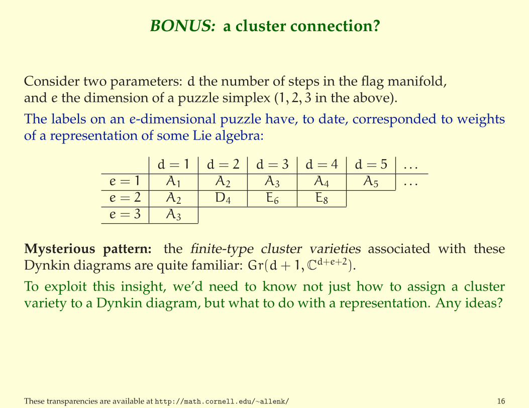
BONUS: a cluster connection?

Consider two parameters: d the number of steps in the flag manifold,and e the dimension of a puzzle simplex (1, 2, 3 in the above).

The labels on an e-dimensional puzzle have, to date, corresponded to weightsof a representation of some Lie algebra:

d = 1 d = 2 d = 3 d = 4 d = 5 . . .e = 1 A1 A2 A3 A4 A5 . . .e = 2 A2 D4 E6 E8

e = 3 A3

Mysterious pattern: the finite-type cluster varieties associated with theseDynkin diagrams are quite familiar: Gr(d+ 1,Cd+e+2).

To exploit this insight, we’d need to know not just how to assign a clustervariety to a Dynkin diagram, but what to do with a representation. Any ideas?


Multiplying Segre-Schwartz-MacPherson classes.

If we keep q around, instead of taking it to ∞, we get classes inKC×(T∗Fl(j, k; Cn)) associated to certain conical-Lagrangian-supported sheaves.Puzzles then compute the products of a related set: those classes, but divided bythe class of the zero section (also Lagrangian). These puzzles also compute (inthe K 99K H∗ limit) the comultiplication of Chern-Schwarz-MacPherson classes.

The Grassmannian rule has puzzle pieces for all nonzero matrix entries ofC

3⊗C3 → Alt2C3; unlike as in ordinary puzzles, this rule doesn’t forbid

the 02 label (those entries are suppressed only in the q→ 0, K 99K H∗ limit).

Theorem [K-ZJ]. The CSM result lets one compute compactly supported Eulercharacteristics of intersections of generically translated Bruhat cells:

χc

(

3⋂

i=1

(gi · X◦λi)

)

= (−1)k(n−k)−∑3

i=1 ℓ(λi) #

{puzzles now including 02 labels

}

Example. Intersect three open Bruhat cells on CP1 transversely,

resulting in CP1 \ {3 points}. That has χc = 2 − 3(1) = −11(2−1),

and indeed there is one puzzle, using the 02 label in the interior. 1

2 0

102

0 201 12


Recognizing quiver varieties that are just T∗Fl(n1, . . . , nd; Cn)).

Obviously if the V dimension vector is supported on a type A subdiagramS ⊆ Q, and W on a single vertex at one end of S, then by the last slideM(Q0, Q1, W , V) ∼= T∗Fl(n1, . . . , nd; C

n). Say that these (V,W) are of flag type.

Nakajima defined “reflections” M(Q0, Q1, W , V, θ) ∼= M(Q0, Q1, W , rα·V, rα·θ)but they involve θ-stability, in general more subtle than our “each ~v ∈ Vi leaksinto some Wj ” stability condition (which corresponds to ∀〈θi, αj〉 > 0).If 〈θi, αj〉 > 0 for all Vj > 0, though, our naıve notion of stability is still correct.

The action of rα · V replaces the α label by the sum of the neighbors includingthe framed neighbor in W , minus the original label. In particular the newdimension is a linear combination of the original dimensions.

Theorem [K-ZJ]. Assume (Q0, Q1, W , V) is of flag type, and thatthe dimensions in π · V are nonnegative combinations of the dimensions in V .Then M(Q0, Q1, W , π · V) ∼= T∗Fl(n1, . . . , nd; C

n)), steps coming from dimV .

Some D4 examples.

n0 j k

0

→

nj j k

j

→

nj j+ k k

j

→

nk j+ k n+ j

k

→

nk n+ k n+ j

k

→

nn n+ k n+ j

k


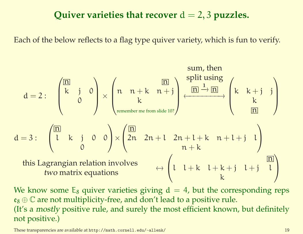
Quiver varieties that recover d = 2, 3 puzzles.

Each of the below reflects to a flag type quiver variety, which is fun to verify.

d = 2 :

nk j 0

0

×

nn n+ k n+ j

k

remember me from slide 10?

sum, thensplit using

n1−→ n

←−−−−−−−→

k k+ j j

k

n

d = 3 :

nl k j 0 0

0

×

n2n 2n+ l 2n+ l+ k n+ l+ j l

n+ k

this Lagrangian relation involvestwo matrix equations

↔

nl l+ k l+ k+ j l+ j l

k

We know some E8 quiver varieties giving d = 4, but the corresponding repse8 ⊕ C are not multiplicity-free, and don’t lead to a positive rule.(It’s a mostly positive rule, and surely the most efficient known, but definitelynot positive.)


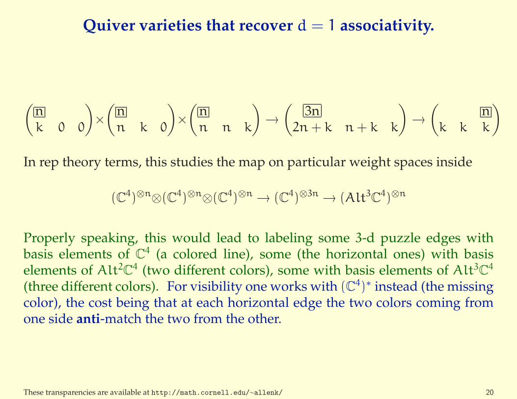
Quiver varieties that recover d = 1 associativity.

(

nk 0 0

)

×

(

nn k 0

)

×

(

nn n k

)

→(

3n2n+ k n+ k k

)

→(

nk k k

)

In rep theory terms, this studies the map on particular weight spaces inside

(C4)⊗n⊗(C4)⊗n⊗(C4)⊗n → (C4)⊗3n → (Alt3C4)⊗n

Properly speaking, this would lead to labeling some 3-d puzzle edges withbasis elements of C

4 (a colored line), some (the horizontal ones) with basiselements of Alt2C4 (two different colors), some with basis elements of Alt3C4

(three different colors). For visibility one works with (C4)∗ instead (the missingcolor), the cost being that at each horizontal edge the two colors coming fromone side anti-match the two from the other.


schubert calculus and quiver varietiespzinn/icr/knutson.pdf · an intersection theory problem. let...

Documents