school of economics working papers · i introduction the implementation of policies aiming to...
TRANSCRIPT

Reducing Public-Private Sector Pay Differentials: The Single Spine Pay Policy as a Natural Experiment in
Ghana
Akwasi Ampofo Firmin Doko Tchatoka
School of Economics, University of Adelaide
Working Paper No. 2018-2 March 2018
Copyright the authors
School of Economics
Working Papers ISSN 2203-6024

Reducing Public-Private Sector Pay Differentials: The
Single Spine Pay Policy as a Natural Experiment in Ghana
Akwasi Ampofo and Firmin Doko Tchatoka∗
School of Economics, The University of Adelaide
ABSTRACT
Empirical studies have documented the existence of the public-private pay differentials in both
developed and developing countries. The implementation of policies aiming to reduce this gap has
however been mitigated or inconclusive. This paper exploits the Single Spine Pay Policy (SSPP)
in Ghana as a natural experiment to examine the effectiveness of wage policies in developing
countries. The SSPP was implemented in 2010 by the Government of Ghana to address the
public-private sector wage gap and improve productivity in the public sector. Using a quantile
treatment effect approach based on a Difference-In-Difference (DID) estimation, we show that
the SSPP has yet to reduce the wage gap between the public and private sectors across the entire
distribution of earnings in Ghana. The improvement observed is only at the lower tail of the
distribution of earnings. However, the SSPP has a larger effect on the earnings of female workers
than that of males in the education and health services sector, suggesting that the policy was
successful in reducing the gender-wage gap in that sector. Moreover, the SSPP has decreased the
productivity of workers across the distribution of earnings, mainly due to a decrease in the effort
of female public sector workers. Nevertheless, the SSPP has had some successes and could be
improved by putting in place a good managerial quality in the government’ agencies. In addition,
it is important that the Government pays much attention to various macroeconomic factors that
have challenged the success of the SSPP.
Key words: Public sector; Efficiency wage theory; Quantile treatment effect model;
DID estimation.
JEL classification: C31, G15, J24, J31, J45.
∗Corresponding author. E-mail: [email protected]. Address: The University of Adelaide,School of Economics, Adelaide, SA 5005, Australia.
1

I Introduction
The implementation of policies aiming to reduce the public-private sector wage gap have received
considerable attention in recent years, especially in developed countries (Lausev 2014). Bregn
(2013) finds that 80 percent of employers in the OECD economies have either implemented such
a wage policy or intended to do so, with the purpose of not only addressing the wage differential
but also to increase workers’ productivity (Bajorek & Bevan 2015). Their success, however, has
been mitigated or inconclusive. While some studies found that adopting a wage policy increases
earnings in the public sector (Hasnain & Pierskalla 2012), their effects on productivity have not
been addressed. Bryson et al. (2012), Lucifora & Origo (2015) argued that wage policies increase
workers’ productivity marginally, but their studies remain silent on how such policies correct
wage disparities between sectors. Most studies on wage gap often focus on the private sector
and little attention is usually paid to the public sector; e.g. (Prentice et al. 2007). Despite
the progress made by many countries in recent years to close the public-private sector wage
gap, the realisation of this goal remains a challenge especially in developing economies. The
few developing countries that implemented wage policies, such as Ghana, have no clear scientific
measure of their success.
This study aims to fill this gap by using the Single Spine Pay Policy (SSPP) in Ghana
as a natural experiment to examine the effects of wage policies in developing countries. In
particular, we investigate whether such a policy reduces the public-private sector wage gap,
while achieving maximum productivity. Using the private sector as a control group, we employ a
quantile treatment effect approach based on a Difference-In-Difference (DID) estimation to show
that the SSPP has yet to reduce the public-private sector wage gap across the entire distribution
of earnings in Ghana. The improvement observed is only at the lower tail of the distribution
of earnings. Nevertheless, the SSPP has a larger effect on the earnings of female workers than
that of males in the public sector, suggesting that the policy was successful in reducing the
gender-wage gap in the public sector. Moreover, the policy has decreased the productivity of
workers across the effort distribution, mainly due to a decrease in the effort of female public
sector workers.
Our findings are similar to Damiani et al. (2016) who estimate a positive policy effect across
the quantiles of earnings and productivity of Italians firms. While, Damiani et al. (2016) find a
2
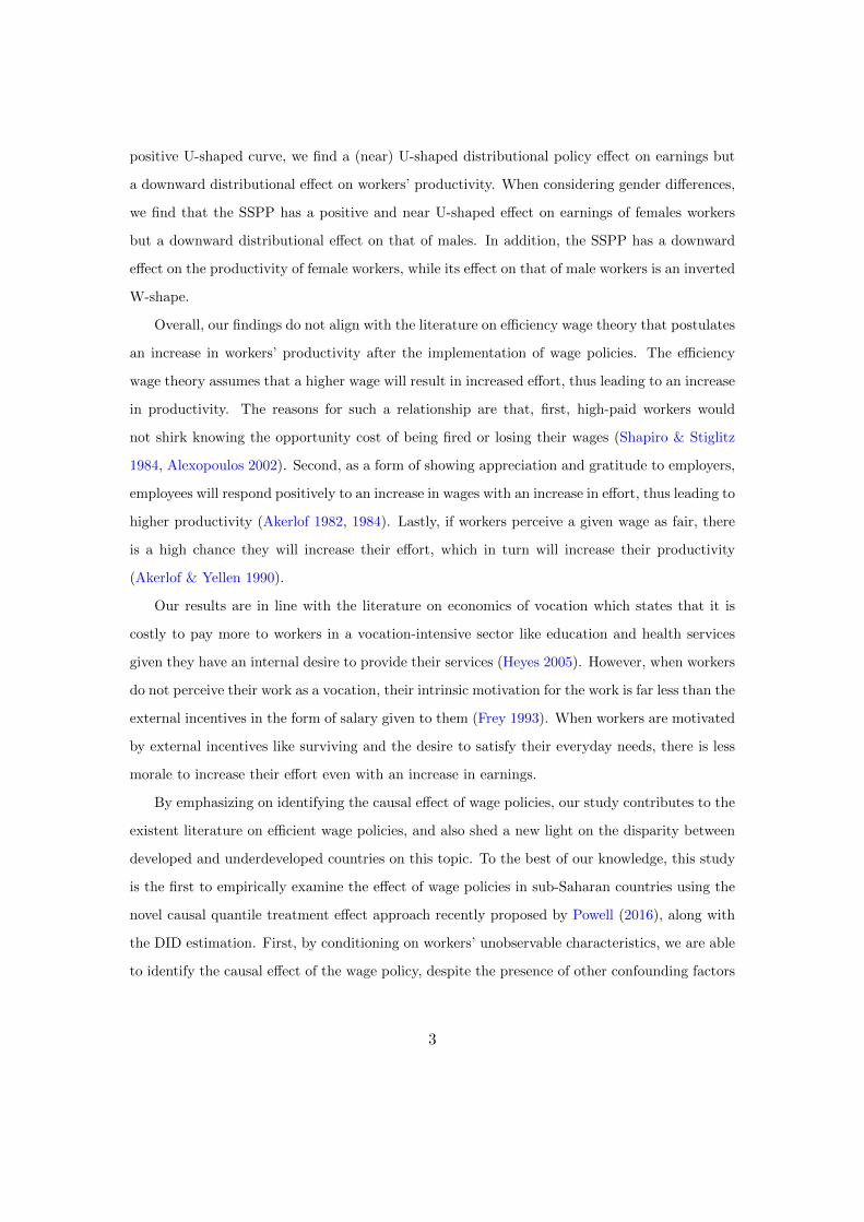
positive U-shaped curve, we find a (near) U-shaped distributional policy effect on earnings but
a downward distributional effect on workers’ productivity. When considering gender differences,
we find that the SSPP has a positive and near U-shaped effect on earnings of females workers
but a downward distributional effect on that of males. In addition, the SSPP has a downward
effect on the productivity of female workers, while its effect on that of male workers is an inverted
W-shape.
Overall, our findings do not align with the literature on efficiency wage theory that postulates
an increase in workers’ productivity after the implementation of wage policies. The efficiency
wage theory assumes that a higher wage will result in increased effort, thus leading to an increase
in productivity. The reasons for such a relationship are that, first, high-paid workers would
not shirk knowing the opportunity cost of being fired or losing their wages (Shapiro & Stiglitz
1984, Alexopoulos 2002). Second, as a form of showing appreciation and gratitude to employers,
employees will respond positively to an increase in wages with an increase in effort, thus leading to
higher productivity (Akerlof 1982, 1984). Lastly, if workers perceive a given wage as fair, there
is a high chance they will increase their effort, which in turn will increase their productivity
(Akerlof & Yellen 1990).
Our results are in line with the literature on economics of vocation which states that it is
costly to pay more to workers in a vocation-intensive sector like education and health services
given they have an internal desire to provide their services (Heyes 2005). However, when workers
do not perceive their work as a vocation, their intrinsic motivation for the work is far less than the
external incentives in the form of salary given to them (Frey 1993). When workers are motivated
by external incentives like surviving and the desire to satisfy their everyday needs, there is less
morale to increase their effort even with an increase in earnings.
By emphasizing on identifying the causal effect of wage policies, our study contributes to the
existent literature on efficient wage policies, and also shed a new light on the disparity between
developed and underdeveloped countries on this topic. To the best of our knowledge, this study
is the first to empirically examine the effect of wage policies in sub-Saharan countries using the
novel causal quantile treatment effect approach recently proposed by Powell (2016), along with
the DID estimation. First, by conditioning on workers’ unobservable characteristics, we are able
to identify the causal effect of the wage policy, despite the presence of other confounding factors
3

which may have contributed to changes in earnings during the period. Second, most studies
of wage policies in the public sector have been limited to workers in the health and education
sectors (Makinson 2000, Prentice et al. 2007). By contrast, our analysis of the wage policy
effectiveness covers the whole public sector. Third, by distinguishing heterogeneous sub-groups
of workers, our results show that the effect of the SSPP is not uniform across these sub-groups.
In particular, while women and low-income workers benefited from the policy, males and high-
income workers did benefit less, which indicates clearly that the mean-type regression analysis,
as often done in the literature, may not be an appropriate way to investigate this type of policies.
Moreover, from a methodological viewpoint, an interesting contribution of our study is the use of
pseudo panels. The absence of genuine panel data covering all areas in Ghana makes it difficult
to have individual observations on workers over time. Following Deaton (1985), we construct a
panel data with individual time-invariant characteristics such as year of birth, gender, and ethnic
composition of workers.
The remainder of the paper is organised as follows. Section II presents the background and
a brief description of the SSPP. Section III introduces the data and the variables used in the
study. Section IV details our empirical strategy. Section V discusses the findings and we present
some robustness checks in Section VI. Section VII concludes.
II The Single Spine Pay Policy in Ghana
Ghana is a West African country with a population of about 27.4 million, with around 49.75 per-
cent of the population being men (World Bank 2017). The economy of Ghana was predominantly
agrarian but recent developments have seen the services and other sectors contributing largely
towards its development. The contribution of the agricultural sector to total GDP (Figure 1a)
has decreased from 49.92 percent in 1965 to 19.60 percent in 2013, while the share of the services
sector has increased from 28.79 to 52.24 percent during the same period (World Bank 2017).
The introduction of democratic rule in 1992, along with subsequent economic reforms, have
spurred the expansion of new enterprises, mostly in the private sector. While this rapid develop-
ment of the private sector has improved earnings for workers, as most private sector employers
pay higher wages, the same is yet to be materialized in the public sector. Several studies have
found that the public-private pay differential was between 15 to 20 percent prior to 2010 (Glewwe
4
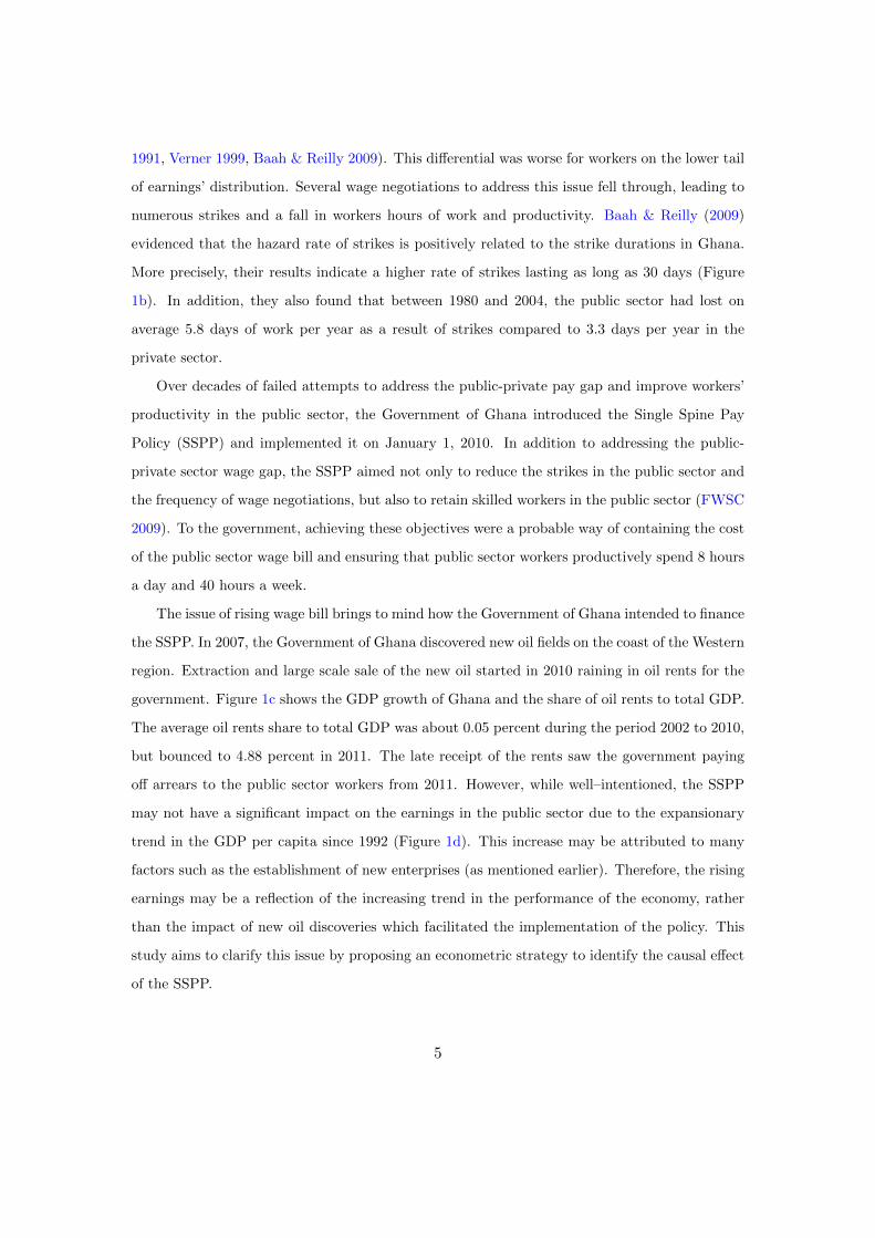
1991, Verner 1999, Baah & Reilly 2009). This differential was worse for workers on the lower tail
of earnings’ distribution. Several wage negotiations to address this issue fell through, leading to
numerous strikes and a fall in workers hours of work and productivity. Baah & Reilly (2009)
evidenced that the hazard rate of strikes is positively related to the strike durations in Ghana.
More precisely, their results indicate a higher rate of strikes lasting as long as 30 days (Figure
1b). In addition, they also found that between 1980 and 2004, the public sector had lost on
average 5.8 days of work per year as a result of strikes compared to 3.3 days per year in the
private sector.
Over decades of failed attempts to address the public-private pay gap and improve workers’
productivity in the public sector, the Government of Ghana introduced the Single Spine Pay
Policy (SSPP) and implemented it on January 1, 2010. In addition to addressing the public-
private sector wage gap, the SSPP aimed not only to reduce the strikes in the public sector and
the frequency of wage negotiations, but also to retain skilled workers in the public sector (FWSC
2009). To the government, achieving these objectives were a probable way of containing the cost
of the public sector wage bill and ensuring that public sector workers productively spend 8 hours
a day and 40 hours a week.
The issue of rising wage bill brings to mind how the Government of Ghana intended to finance
the SSPP. In 2007, the Government of Ghana discovered new oil fields on the coast of the Western
region. Extraction and large scale sale of the new oil started in 2010 raining in oil rents for the
government. Figure 1c shows the GDP growth of Ghana and the share of oil rents to total GDP.
The average oil rents share to total GDP was about 0.05 percent during the period 2002 to 2010,
but bounced to 4.88 percent in 2011. The late receipt of the rents saw the government paying
off arrears to the public sector workers from 2011. However, while well–intentioned, the SSPP
may not have a significant impact on the earnings in the public sector due to the expansionary
trend in the GDP per capita since 1992 (Figure 1d). This increase may be attributed to many
factors such as the establishment of new enterprises (as mentioned earlier). Therefore, the rising
earnings may be a reflection of the increasing trend in the performance of the economy, rather
than the impact of new oil discoveries which facilitated the implementation of the policy. This
study aims to clarify this issue by proposing an econometric strategy to identify the causal effect
of the SSPP.
5

FIGURE 1: Economic Indicators and Strikes Duration in Ghanaian
(a) Sector Share of GDP(b) Hazard rates of strike duration in Ghana from
Baah & Reilly (2009).
(c) GDP Growth in Ghana (d) GDP per capita at 2010 constant US prices
III Data
We use data from the Ghana Living Standard Survey (GLSS), rounds 4,5 and 6 conducted in
1998, 2006 and 2013 respectively. This means there are two pre-policy (1998, 2006) and one
post-policy (2013) data points. This is a national representative and one of the largest repeated
cross-section dataset with 5998 households in 1998, 8687 in 2006, and 16772 in 2013, surveyed
across the 10 regions of Ghana (Ghana Statistical Service 2016)1. The data include household
socioeconomic characteristics and a roster of members in the household, their employment status,
their sector of work, their earnings, their hours of works, their ages and educational attainment,
ethnic composition and other demographic variables. We restrict our sample to only respondents
1The GLSS has a wider coverage than the Ghana Household Urban Population Survey which is a panel andcovers only the urban cities in Ghana.
6

above 15 years2 and employed.
As the GLSS is a repeated cross-section data, the unavailability of a panel form makes it
difficult to follow the respondents over time. We tackle this challenge by constructing a pseudo
panel (Deaton 1985). The approach is such that respondents are grouped into cohorts accord-
ing to the same time invariant characteristics that identify them. We then compute averages
of continuous time-varying variables for each cohort across each survey and used them as ob-
servations. Discrete time varying variables like marital status and household status (head or
not) are, however, used as reported because they are considered to be rid of errors (Deaton
1985). The individual fixed effect which identifies the unobserved heterogeneity in a panel data
is then referred to as a cohort fixed effect. Though this is not necessarily following individuals
over time but rather cohorts, it makes it possible to infer individuals’ behavior from a group
with similar characteristics. In the literature, the widely used time-invariant characteristics to
construct cohorts have been the birth year and gender. We use these variables for the reasons
that they depict the life-cycle and existing wage differentials between and among workers. The
well-known Mincer (1974) wage equation considers age (experience) as an important determinant
of earnings, and this was proven to be the case in Ghana (Glewwe 1991). Glewwe (1991) found
that the age-earning profile depicts the experience and earning profile of workers, and that even
within the same age-earning profile, there exists a pay differential by gender. Various studies,
Newell & Reilly (1996), Cohen & Huffman (2007) and Aizer (2010) also found that the gender
wage gap exists in both developed and developing countries, mostly in favor of men.
In addition to year of birth and gender, we also construct cohorts using the ethnic composition
of the respondents. The use of the ethnic composition to construct cohorts is inspired by Easterly
& Levine (1997), who investigated the effect of ethnic diversity on economic development in
both developed and developing countries. They found that diversity of ethnic backgrounds in
most countries (developed and developing) influences the differences in income and productivity.
Easterly & Levine (1997) argue that these differences arise from various innate capabilities that
characterise each ethnic group, making ethnicity an important factor to consider when estimating
earnings and productivity.
The Ghanaian population is very diverse with different ethnic groups. This diversity affect
2This is because by the International Labour Law, working at age below 15 years is a child labour.
7
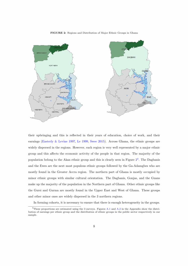
FIGURE 2: Regions and Distribution of Major Ethnic Groups in Ghana
their upbringing and this is reflected in their years of education, choice of work, and their
earnings (Easterly & Levine 1997, Le 1999, Swee 2015). Across Ghana, the ethnic groups are
widely dispersed in the regions. However, each region is very well represented by a major ethnic
group and this affects the economic activity of the people in that region. The majority of the
population belong to the Akan ethnic group and this is clearly seen in Figure 23. The Dagbanis
and the Ewes are the next most populous ethnic groups followed by the Ga-Adamgbes who are
mostly found in the Greater Accra region. The northern part of Ghana is mostly occupied by
minor ethnic groups with similar cultural orientation. The Dagbanis, Gonjas, and the Guans
make up the majority of the population in the Northern part of Ghana. Other ethnic groups like
the Gursi and Gurma are mostly found in the Upper East and West of Ghana. These groups
and other minor ones are widely dispersed in the 3 northern regions.
In forming cohorts, it is necessary to ensure that there is enough heterogeneity in the groups.
3These proportions are estimated using the 3 surveys. Figures A.1 and A.2 in the Appendix show the distri-bution of earnings per ethnic group and the distribution of ethnic groups in the public sector respectively in oursample.
8

This requirement calls for larger cohort size and groups. The restriction on the available data
makes it difficult to ensure these two requirements are satisfied, which usually leads to a trade-
off between efficiency and bias. This is because a larger cohort size will reduce the number of
groups (thus rendering the estimates efficient but biased), whereas a small cohort size and a
larger number of groups will result in less efficient estimates but rid of bias. Verbeek & Nijman
(1992) note that the main problem of cohort fixed effect is that it is time-varying, unobserved
and very likely to be correlated with the averages of the variables. With the average cohort effect
varying over time, treating them as random will result in inconsistent estimates, and treating
them as fixed will lead to identification problems unless the variation of the cohort effect over
time can be neglected. However, with cohorts sizes of at least 100, there is a chance of having the
errors resulting from averaging the variables being neglected, and the estimates being consistent
(Verbeek & Nijman 1992).
We form the cohorts, first, by combining all ethnic groups with less than 1,000 respondents
as “Others.” This group together with the Akan, Ewe, Ga-Adamgbe, Guan and Mole-Dagbani
make up 6 ethnic groups. We then form the year of birth cohort by using different year intervals
(25, 16, 6) so as to have an equal proportion (16 percent) of respondents in each cohort. Using
equal year intervals will leave some year cohorts with fewer respondents. We finally form the
cohorts from 6 ethnic groups, 6 birth years and 2 gender groups giving us 72 groups4 in each
survey. Sixteen (16) percent of the total created cohorts have less than 100 respondents; this is
tolerable from the literature on pseudo panel construction.
IV Empirical Strategy
To identify the effect of the SSPP, we use a quantile treatment approach along with a Difference-
In-Difference (DID) estimation. Section A details the specification used, while Section B discusses
briefly the identification issues related to this type of models.
4 Other groups were also constructed but most of the cohorts size were less than 100 and had lessheterogeneity in them. Details of the variables used are included in Tables A.1-A.4 of the Appendix.
9
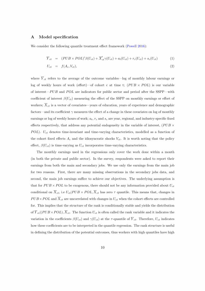
A Model specification
We consider the following quantile treatment effect framework (Powell 2016):
Y ct = (PUB × POL)′β(Uct) +X′ctγ(Uct) + at(Uct) + rc(Uct) + sc(Uct) (1)
Uct = f(Ac, Vct), (2)
where Y ct refers to the average of the outcome variables—log of monthly labour earnings or
log of weekly hours of work (effort)—of cohort c at time t; (PUB × POL) is our variable
of interest—PUB and POL are indicators for public sector and period after the SSPP—with
coefficient of interest β(Uct) measuring the effect of the SSPP on monthly earnings or effort of
workers; Xct is a vector of covariates—years of education, years of experience and demographic
factors—and its coefficient γ measures the effect of a change in these covariates on log of monthly
earnings or log of weekly hours of work; at, rc and sc are year, regional, and industry-specific fixed
effects respectively, that address any potential endogeneity in the variable of interest, (PUB ×
POL). Uct denotes time-invariant and time-varying characteristics, modelled as a function of
the cohort fixed effects Ac and the idiosyncratic shocks Vct. It is worth noting that the policy
effect, β(Uct) is time-varying as Uct incorporates time-varying characteristics.
The monthly earnings used in the regressions only cover the work done within a month
(in both the private and public sector). In the survey, respondents were asked to report their
earnings from both the main and secondary jobs. We use only the earnings from the main job
for two reasons. First, there are many missing observations in the secondary jobs data, and
second, the main job earnings suffice to achieve our objectives. The underlying assumption is
that for PUB × POL to be exogenous, there should not be any information provided about Uct
conditional on Xct, i.e Uct|PUB × POL,Xct has zero τ quantile. This means that, changes in
PUB×POL and Xct are uncorrelated with changes in Uct when the cohort effects are controlled
for. This implies that the structure of the rank is conditionally stable and yields the distribution
of Y ct|(PUB×POL), Xct. The function Uct is often called the rank variable and it indicates the
variation in the coefficients β(Uct) and γ(Uct) at the τ -quantile of Y ct. Therefore, Uct indicates
how these coefficients are to be interpreted in the quantile regression. The rank structure is useful
in defining the distribution of the potential outcomes, thus workers with high quantiles have high
10

value of Uct which is a function of their cohort and idiosyncratic effects. The assumption on the
rank structure is commonly used in the literature, and allows for recovering the joint distribution
from the marginal ones. Each observation is assumed to maintain its rank in the distribution of
earnings and effort regardless of the treatment status so that the estimated effect is the treatment
effect for observations at the quantile of the potential outcome distributions (Melly & Wuthrich
2016). This rank assumption is different from that with additive fixed effects. While the former
yields the estimation of the distribution of Y ct|PUB×POL,Xct, the latter approach only yields
the estimation on the distribution of (Y ct − Uct)|PUB × POL,Xct. This means that in the
latter, individuals at the bottom of the distribution (Y ct−Uct)|PUB×POL,Xct may be closer
to the top of the distribution Y ct|PUB × POL,Xct, thus contradicting the rank assumption.
Interestingly, Powell (2016) methodology of estimating the quantiles of Y ct|PUB × POL,Xct
yields consistent estimates even for short T (T = 3 in this study), which is an advantage over
quantile regressions with additive fixed effects that require large T .
Conditioning on covariates like educational attainment and years of experience matters in the
determination of earnings and productivity; e.g., Mincer (1974), Glewwe (1991), and Adamchik
& Bedi (2000). Other factors like marital status, household head status, and father’s working
status also influence earnings (Le 1999). Ignoring these variables will result in a misspecified
model, thus leading to imprecise estimates (Powell 2016).
The year fixed effects help in capturing various economic and political happenings that have
evolved over time. Ignoring the activities of government which could in a way influence the
earnings of workers will affect the identification of the policy effect. One interesting factor that
made it possible for the implementation of the policy was the availability of an extra source of
funding for the government as a result of an oil discovery in 2007. A new source of funding was
needed as the government did not have stored up funds to embark on such a huge expenditure.
The performance of the economy prior to the SSPP implementation, as noted by the World
Bank, was declining with an annual growth rate averaging 6 percent. The growth rate increased
from 5 percent in 2010 to 14 percent in 2011 (Figure 1c, Section 2) and declined to 9 percent
the following year World Bank (2017). This shock could be attributed to the discovery and
extraction of new oil fields from 2010. This discovery may make the policy endogenous and
not accounting for this may result in an inefficient estimation of the policy effect. One way to
11
address this, is to have a time dummy for the period of the oil discovery. The data available does
not allow to have a different time dummy for the period after oil discovery and the pay policy.
However, the inclusion of the year fixed effect helps to address this problem. Another way is the
inclusion of regional effects which will account for the economic activities that evolved after the
oil discovery.
The inclusion of the cohort fixed effect and industry-specific fixed effect is of essence as this helps
in not attributing the effect of time invariant traits to the policy.
The literature on efficiency wages considers working hours as a measure of effort. (Katz
1986, Campbell 2006). Effort, according to the literature, is positively related to the level of
productivity of a firm or an individual. In Ghana, workers are by law5 required to work 8 hours
a day and 40 hours a week for a full time work. This is admonished in the public sector and it
was a reason for the government agreeing to a new pay policy. The believe is that, effectively
working within this stipulated hours will result in higher level of productivity and result in a
cut in employment in the public sector. This institutional setting renders it possible to measure
the effort of workers, thus their level of productivity, through hours of work. Considering the
unavailability of a better measure of productivity from the individual data, and more importantly
the underlying theory, we use hours of work as an ‘indirect ’ measure of productivity. We propose
two approaches in measuring effort. First, we use log of weekly hours of work. This approach is
deemed appropriate as it is easier to capture a possible change in effort on average and also at
the quantiles. Next we use a dummy that takes 1 if an individual works at least 40 hours a week
(more productive worker) and 0 otherwise (less productive worker).
We estimate the DID model using the Generalized Methods of Moments(GMM) approach
by Powell (2016) with two moment conditions. The first is the within transformation of the
data which ensures that the within cohorts comparison is used for identification. The second
moment condition ensures that, on average, the expected probability of each cohort is equal to
the quantile function. The two moment conditions can be written formally as:
E
{1
2T 2
T∑t=1
T∑s=1
(Zct − Zcs)[1(Y ct ≤ q(Dct, τ))− 1(Y cs ≤ q(Dcs, τ))
]}= 0 (3)
E[1(Y ct ≤ q(Dct, τ))− τ
]= 0, (4)
5See Ghanian Labour Act 2003, Section on hours of work.
12

where Zct and Zcs are instruments in cohort c at time t and s, D is the treatment variable,
PUB×POL , τ is the τ -quantile of Y ct, and q(Dcs, τ) is a strictly increasing function of τ . The
GMM estimator obtained by using the two moments conditions in (1)–(2) may be difficult to
compute. Powell (2016) proposes to use the following equivalent moment conditions:
E
[1
T
T∑t=1
(Zct − Zc)[1(Y ct ≤ q(Dct, τ))
]]= 0 (5)
E[1(Y ct ≤ q(Dct, τ))− τ
]= 0, (6)
where Zc = 1T
∑Tt=1 Zct. The GMM estimator of β(τ) and γ(τ) in (1)–(2) solves the minimization
problem
minb∈B
Q(b) : Q(b) = m(b)′W (b)m(b), (7)
m(b) =1
N
N∑c=1
mc(b), mc(b) =
1T
∑Tt=1(Zct − Zc)
[1(Y ct ≤ D′
ctb)]
1T
∑Tt=1 1(Y ct ≤ D′
ctb)− τ
,where B =
{b : τ − 1
N < 1N
∑Nc=1 1(Y ct ≤ D′
ctb) ≤ τ for all t}, b ≡ [β(τ)
′, γ(τ)
′]′, W (b) is a
weighting matrix, and N is the size of cohorts. Restricting the parameters to B guarantees that
the condition Y ct ≤ D′ctb holds for (approximately) 100τ% of the observations in each time
period. We use the Markov Chain Monte Carlo algorithm (MCMC) to solve the optimization
problem, as suggested by Powell (2016).
B Threat to Identifying a Significant Policy Effect
The source of a policy variation needs to be understood better in order to avoid making erroneous
inferences (Besley & Case 2000). A change in the monthly earnings and weekly hours of work
could be as a result of series of factors but not necessarily the policy. Also, an important factor
to consider is the control group with which the treated group is being compared to. The private
sector is an equally viable option for public sector workers provided they find their efforts not
to be rewarded accordingly. We use the private sector as a control group because there is a fear
that the government will lose its workers to this sector, but not the other way around (FWSC
2009). Although there is job security in the public sector, the monetary gain is a clear cut for
13
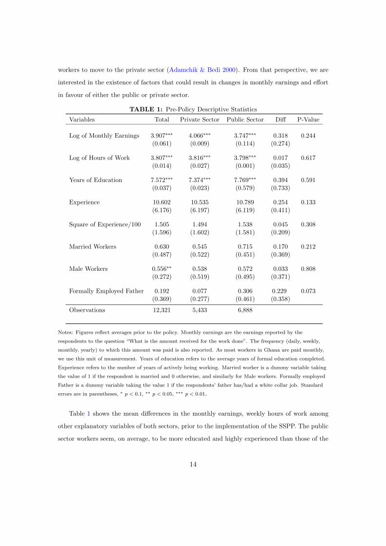
workers to move to the private sector (Adamchik & Bedi 2000). From that perspective, we are
interested in the existence of factors that could result in changes in monthly earnings and effort
in favour of either the public or private sector.
TABLE 1: Pre-Policy Descriptive Statistics
Variables Total Private Sector Public Sector Diff P-Value
Log of Monthly Earnings 3.907∗∗∗ 4.066∗∗∗ 3.747∗∗∗ 0.318 0.244(0.061) (0.009) (0.114) (0.274)
Log of Hours of Work 3.807∗∗∗ 3.816∗∗∗ 3.798∗∗∗ 0.017 0.617(0.014) (0.027) (0.001) (0.035)
Years of Education 7.572∗∗∗ 7.374∗∗∗ 7.769∗∗∗ 0.394 0.591(0.037) (0.023) (0.579) (0.733)
Experience 10.602 10.535 10.789 0.254 0.133(6.176) (6.197) (6.119) (0.411)
Square of Experience/100 1.505 1.494 1.538 0.045 0.308(1.596) (1.602) (1.581) (0.209)
Married Workers 0.630 0.545 0.715 0.170 0.212(0.487) (0.522) (0.451) (0.369)
Male Workers 0.556∗∗ 0.538 0.572 0.033 0.808(0.272) (0.519) (0.495) (0.371)
Formally Employed Father 0.192 0.077 0.306 0.229 0.073(0.369) (0.277) (0.461) (0.358)
Observations 12,321 5,433 6,888
Notes: Figures reflect averages prior to the policy. Monthly earnings are the earnings reported by the
respondents to the question “What is the amount received for the work done”. The frequency (daily, weekly,
monthly, yearly) to which this amount was paid is also reported. As most workers in Ghana are paid monthly,
we use this unit of measurement. Years of education refers to the average years of formal education completed.
Experience refers to the number of years of actively being working. Married worker is a dummy variable taking
the value of 1 if the respondent is married and 0 otherwise, and similarly for Male workers. Formally employed
Father is a dummy variable taking the value 1 if the respondents’ father has/had a white collar job. Standard
errors are in parentheses, ∗ p < 0.1, ∗∗ p < 0.05, ∗∗∗ p < 0.01.
Table 1 shows the mean differences in the monthly earnings, weekly hours of work among
other explanatory variables of both sectors, prior to the implementation of the SSPP. The public
sector workers seem, on average, to be more educated and highly experienced than those of the
14

private sector, but such differences are statistically insignificant to contribute to any change in
the monthly earnings and weekly hours of work. A closer look at the income and effort of workers
reveal the story about unfolding. Figure 3 depicts the earnings of workers before and after the
policy. There is an increase in the earnings of the public sector but their weekly hours of work
have decreased marginally after the SSPP was implemented. The distribution of the earnings in
these two sectors, as depicted show that the public sector earnings are concentrated around the
mean after the policy was introduced, with a reduction in the distribution towards the lower tail.
This indicates homogeneity in the earnings of most workers in that sector, and similarly for the
private sector. Regarding the weekly hours of work in Figure 4, the distribution did not change
much for both sectors but a large fraction of workers have their weekly hours of work close to the
mean after the SSPP was implemented. This, however, may not be enough in establishing the
absence of selections on unobservable factors. We thus conduct placebo tests, as well as other
robustness checks in section B to ensure the estimates are well identified.
15

FIGURE 3: Distribution of Monthly Earnings
16
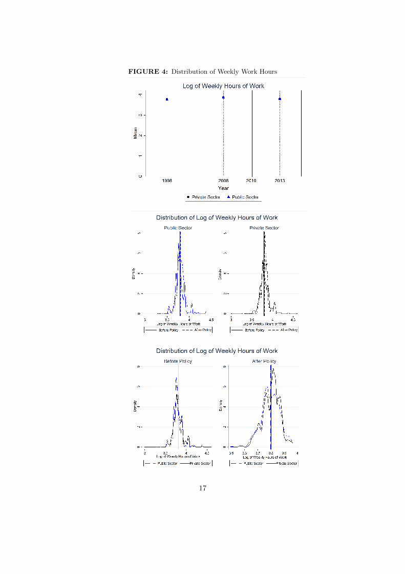
FIGURE 4: Distribution of Weekly Work Hours
17

V Results
For clarity, we present the effects of the SSPP on earnings and effort on separate sections.
A Policy Effect on Earnings
Table 2 shows the estimates of the policy effect on log of monthly earnings. The OLS and
pooled quantile estimates based on Koenker & Bassett Jr (1978) are presented in Table 2.I
and Table 2.II, whereas Table 2.III shows the quantile fixed effect (QRPD) estimates using the
approach by Powell (2016). The estimates in Table 2.I with no individual controls and cohort
effects suggest the SSPP has a positive and statistically significant effect on average, and also
across the earnings distribution, except at the 90th quantile. Including controls for workers’
education, years of experience, marital status, presence of union at place of work, household
status (head or not), and fathers’ choice of work (white collar job or not), reduces the policy
effect on average and also across quantiles of the distribution (Table 2.II). The reduction in the
effect of the SSPP after the inclusion of control variables indicates the role individual factors
play in determining earnings. Across the quantiles of the log of monthly earnings, the SSPP had
its highest effect at the lower tail of the distribution and the impact decreases gradually as the
quantiles increase. Figure 5 shows the graphs of the estimates in Table 2.II. The DID estimates
are on the y-axis and the quantiles of log of monthly earnings on the x -axis. The effect of the
policy is significantly above and below the average effect (OLS), indicating the heterogeneous
nature of the policy on the monthly earnings in the public sector.
These effects, however, reduces with the inclusion of the cohort fixed effects as shown in
Table 2.III and in Figure 5. The inclusion of the cohort fixed effect indicates that omitting
the unobserved heterogeneity arising from the year of birth, the gender and ethnic composition,
will bias the effect of the SSPP upwards. Another significant result is that the effect of the
SSPP is positive on average but negative and significant beyond the median quantile; indicating
a negative effect on the earnings of public sector workers. Whereas the SSPP increased the
monthly earnings of public sector workers at the 10th quantile by 21.45 and 13.24 percentage
points for workers at the 25th quantile, it reduced the monthly earnings of public sector workers
at the 75th quantile by 0.56 and 0.48 percentage points for those at the 90th quantile.
Table 2 also shows the public-private earnings gap in the absence of the SSPP. The first row of
18
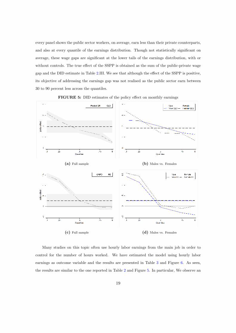
every panel shows the public sector workers, on average, earn less than their private counterparts,
and also at every quantile of the earnings distribution. Though not statistically significant on
average, these wage gaps are significant at the lower tails of the earnings distribution, with or
without controls. The true effect of the SSPP is obtained as the sum of the public-private wage
gap and the DID estimate in Table 2.III. We see that although the effect of the SSPP is positive,
its objective of addressing the earnings gap was not realised as the public sector earn between
30 to 90 percent less across the quantiles.
FIGURE 5: DID estimates of the policy effect on monthly earnings
(a) Full sample (b) Males vs. Females
(c) Full sample (d) Males vs. Females
Many studies on this topic often use hourly labor earnings from the main job in order to
control for the number of hours worked. We have estimated the model using hourly labor
earnings as outcome variable and the results are presented in Table 3 and Figure 6. As seen,
the results are similar to the one reported in Table 2 and Figure 5. In particular, We observe an
19
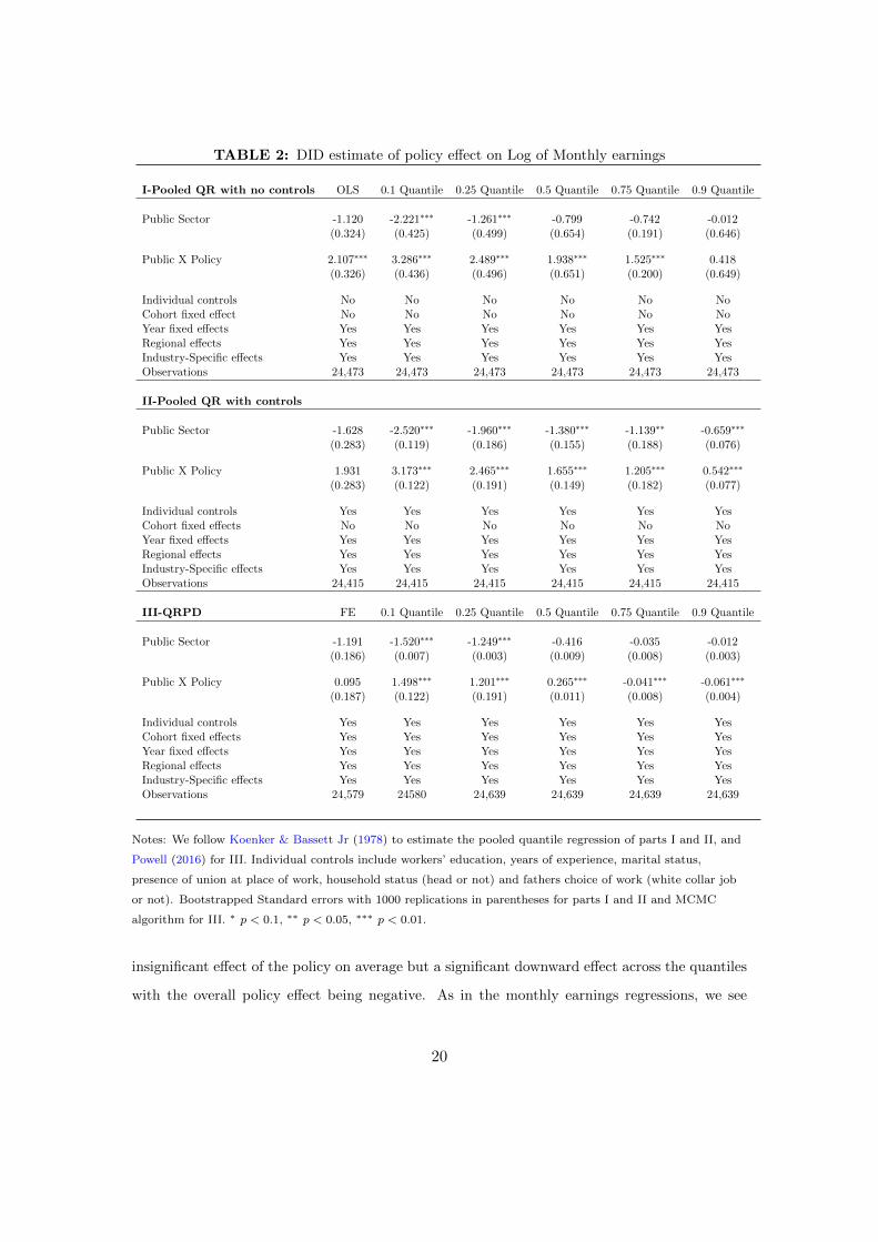
TABLE 2: DID estimate of policy effect on Log of Monthly earnings
I-Pooled QR with no controls OLS 0.1 Quantile 0.25 Quantile 0.5 Quantile 0.75 Quantile 0.9 Quantile
Public Sector -1.120 -2.221∗∗∗ -1.261∗∗∗ -0.799 -0.742 -0.012(0.324) (0.425) (0.499) (0.654) (0.191) (0.646)
Public X Policy 2.107∗∗∗ 3.286∗∗∗ 2.489∗∗∗ 1.938∗∗∗ 1.525∗∗∗ 0.418(0.326) (0.436) (0.496) (0.651) (0.200) (0.649)
Individual controls No No No No No NoCohort fixed effect No No No No No NoYear fixed effects Yes Yes Yes Yes Yes YesRegional effects Yes Yes Yes Yes Yes YesIndustry-Specific effects Yes Yes Yes Yes Yes YesObservations 24,473 24,473 24,473 24,473 24,473 24,473
II-Pooled QR with controls
Public Sector -1.628 -2.520∗∗∗ -1.960∗∗∗ -1.380∗∗∗ -1.139∗∗ -0.659∗∗∗
(0.283) (0.119) (0.186) (0.155) (0.188) (0.076)
Public X Policy 1.931 3.173∗∗∗ 2.465∗∗∗ 1.655∗∗∗ 1.205∗∗∗ 0.542∗∗∗
(0.283) (0.122) (0.191) (0.149) (0.182) (0.077)
Individual controls Yes Yes Yes Yes Yes YesCohort fixed effects No No No No No NoYear fixed effects Yes Yes Yes Yes Yes YesRegional effects Yes Yes Yes Yes Yes YesIndustry-Specific effects Yes Yes Yes Yes Yes YesObservations 24,415 24,415 24,415 24,415 24,415 24,415
III-QRPD FE 0.1 Quantile 0.25 Quantile 0.5 Quantile 0.75 Quantile 0.9 Quantile
Public Sector -1.191 -1.520∗∗∗ -1.249∗∗∗ -0.416 -0.035 -0.012(0.186) (0.007) (0.003) (0.009) (0.008) (0.003)
Public X Policy 0.095 1.498∗∗∗ 1.201∗∗∗ 0.265∗∗∗ -0.041∗∗∗ -0.061∗∗∗
(0.187) (0.122) (0.191) (0.011) (0.008) (0.004)
Individual controls Yes Yes Yes Yes Yes YesCohort fixed effects Yes Yes Yes Yes Yes YesYear fixed effects Yes Yes Yes Yes Yes YesRegional effects Yes Yes Yes Yes Yes YesIndustry-Specific effects Yes Yes Yes Yes Yes YesObservations 24,579 24580 24,639 24,639 24,639 24,639
Notes: We follow Koenker & Bassett Jr (1978) to estimate the pooled quantile regression of parts I and II, and
Powell (2016) for III. Individual controls include workers’ education, years of experience, marital status,
presence of union at place of work, household status (head or not) and fathers choice of work (white collar job
or not). Bootstrapped Standard errors with 1000 replications in parentheses for parts I and II and MCMC
algorithm for III. ∗ p < 0.1, ∗∗ p < 0.05, ∗∗∗ p < 0.01.
insignificant effect of the policy on average but a significant downward effect across the quantiles
with the overall policy effect being negative. As in the monthly earnings regressions, we see
20
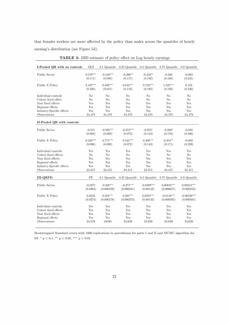
that females workers are more affected by the policy than males across the quantiles of hourly
earning’s distribution (see Figure 5d).
TABLE 3: DID estimate of policy effect on Log hourly earnings
I-Pooled QR with no controls OLS 0.1 Quantile 0.25 Quantile 0.5 Quantile 0.75 Quantile 0.9 Quantile
Public Sector 0.579∗∗∗ -0.549∗∗∗ -0.296∗∗ -0.434∗∗ -0.226 -0.063(0.111) (0.048) (0.117) (0.192) (0.180) (0.231)
Public X Policy 2.107∗∗∗ 0.839∗∗∗ 0.643∗∗∗ 0.742∗∗∗ 1.525∗∗∗ 0.123(0.326) (0.051) (0.116) (0.192) (0.180) (0.230)
Individual controls No No No No No NoCohort fixed effect No No No No No NoYear fixed effects Yes Yes Yes Yes Yes YesRegional effects Yes Yes Yes Yes Yes YesIndustry-Specific effects Yes Yes Yes Yes Yes YesObservations 24,473 24,473 24,473 24,473 24,473 24,473
II-Pooled QR with controls
Public Sector -0.315 -0.595∗∗∗ -0.372∗∗∗ -0.253∗ -0.289∗ -0.050(0.095) (0.098) (0.072) (0.143) (0.170) (0.206)
Public X Policy 0.428∗∗∗ 0.771∗∗∗ 0.545∗∗∗ 0.408∗∗∗ 0.354∗∗ -0.003(0.096) (0.099) (0.072) (0.143) (0.171) (0.209)
Individual controls Yes Yes Yes Yes Yes YesCohort fixed effects No No No No No NoYear fixed effects Yes Yes Yes Yes Yes YesRegional effects Yes Yes Yes Yes Yes YesIndustry-Specific effects Yes Yes Yes Yes Yes YesObservations 24,415 24,415 24,415 24,415 24,415 24,415
III-QRPD FE 0.1 Quantile 0.25 Quantile 0.5 Quantile 0.75 Quantile 0.9 Quantile
Public Sector -0.0271 -0.328∗∗∗ -0.271∗∗∗ -0.0289∗∗∗ 0.00845∗∗∗ 0.00215∗∗∗
(0.0364) (0.000193) (0.000341) (0.00142) (0.000657) (0.000452)
Public X Policy 0.0223 0.324∗∗∗ 0.265∗∗∗ 0.0232∗∗∗ -0.0110∗∗∗ -0.00538∗∗∗
(0.0374) (0.000178) (0.000373) (0.00132) (0.000585) (0.000501)
Individual controls Yes Yes Yes Yes Yes YesCohort fixed effects Yes Yes Yes Yes Yes YesYear fixed effects Yes Yes Yes Yes Yes YesRegional effects Yes Yes Yes Yes Yes YesObservations 24,579 24580 24,639 24,639 24,639 24,639
Bootstrapped Standard errors with 1000 replications in parentheses for parts I and II and MCMC algorithm for
III. ∗ p < 0.1, ∗∗ p < 0.05, ∗∗∗ p < 0.01.
21
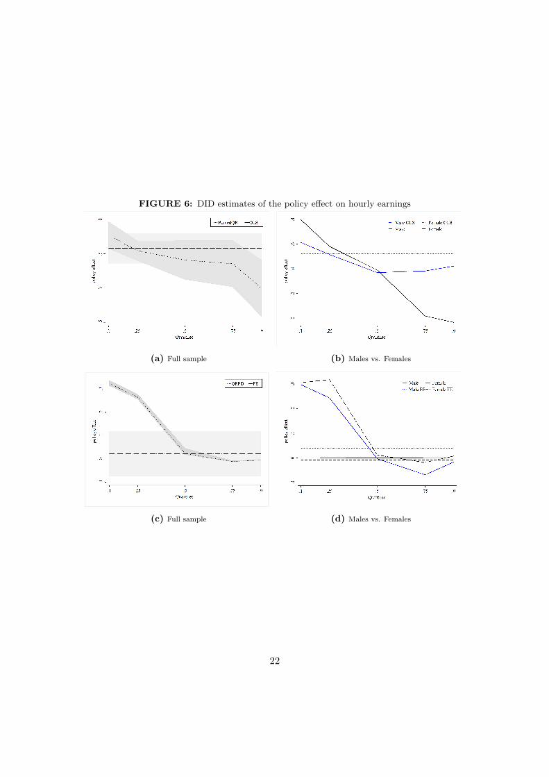
FIGURE 6: DID estimates of the policy effect on hourly earnings
(a) Full sample (b) Males vs. Females
(c) Full sample (d) Males vs. Females
22

B Policy Effect on Effort
We examine the effect of the SSPP on the effort of public sector workers. The estimates using
the log of hours of work as outcome variable is presented in Table 4. As before, the OLS and
pooled quantile estimates based on Koenker & Bassett Jr (1978) are presented in (Table 4.I)
and (Table 4.II) respectively, whereas Table 4.III shows the fixed effect QRPD estimates using
the approach by Powell (2016). The DID estimates with no individual controls and cohort fixed
effects are positive and significant on average and also at the 10th quantile, but negative and
significant at the 90th quantile of weekly hours. This indicates a fall in the effort of public sector
workers after the implementation of the SSPP.
The inclusion of individual controls reduces the effect of the wage policy on public sector
effort on average and also at the 10th quantile. The effect, however, is negative from the median
and only statistically significant at the 90th quantile (Table 4.II). Moreover, the SSPP effect
on the effort of public sector workers reduces and turn negative on average and also beyond
the median after including the cohort fixed effect (Table 4.III). Figure 7 shows the SSPP effect
on the effort of workers. There is a significant effect of the SSPP below and above the average
indicating that the heterogeneous effect across the quantiles is informative as an average estimate
will disregard the reduction in effort of workers at higher tails of the effort distribution.
Like in the case of monthly earnings, the SSPP did not achieve its objective of ensuring
an increase in the effort and in turn the productivity in the public sector. The public-private
effort gap, without the policy, is significantly positive on average and also at the 90th quantile
(Table 4.III). The public sector reduced their effort by 0.4 percent on average and between 0.1
and 0.3 percent across the quantiles after the implementation of the SSPP.
An alternative approach to test for the effectiveness of the SSPP on effort is to use a dummy
variable taking a value of 1 if an individual works 40 hours or more a week, and 0 otherwise. We
find that the SSPP has, on average, insignificantly reduced the effort of public sector work by
around 10 percent (Table A.6).
23

TABLE 4: DID estimate of the SSPP effects on weekly hours of work
I-Pooled QR with no controls OLS 0.1 Quantile 0.25 Quantile 0.5 Quantile 0.75 Quantile 0.9 Quantile
Public Sector -0.137 -0.588∗∗∗ -0.154 -0.134 -0.056 0.125(0.082) (0.100) (0.125) (0.155) (0.144) (0.124)
Public X Policy 0.144∗ 0.927∗∗∗ 0.154 0.093 0.150 -0.279∗∗
(0.083) (0.114) (0.126) (0.158) (0.145) (0.127)
Individual controls No No No No No NoCohort fixed effect No No No No No NoYear fixed effects Yes Yes Yes Yes Yes YesRegional effects Yes Yes Yes Yes Yes YesIndustry-Specific effects Yes Yes Yes Yes Yes YesObservations 23,981 23,981 23,981 23,981 23,981 23,981
II-Pooled QR with controls
Public Sector -0.160∗∗ -0.621∗∗∗ -0.087∗∗∗ 0.087∗∗∗ -0.013 0.047∗∗∗
(0.082) (0.068) (0.164) (0.214) (0.137) (0.043)
Public X Policy 0.117∗ 0.744∗∗∗ 0.054 -0.195 -0.214 -0.198∗∗∗
(0.083) (0.071) (0.165) (0.216) (0.138) (0.046)
Individual controls Yes Yes Yes Yes Yes YesCohort fixed effects No No No No No NoYear fixed effects Yes Yes Yes Yes Yes YesRegional effects Yes Yes Yes Yes Yes YesIndustry-Specific effects Yes Yes Yes Yes Yes YesObservations 23,927 23,927 23,927 23,927 23,927 23,927
III-QRPD
Public Sector 0.051∗∗∗ -0.049 -0.004 0.027 0.041 0.104∗∗
(0.014) (0.000) (0.000) (0.028) (0.003) (0.043)
Public X Policy -0.055∗∗∗ 0.048∗∗∗ 0.0005 -0.028∗∗∗ -0.041∗∗ -0.108∗∗∗
(0.014) (0.003) (0.007) (0.009) (0.005) (0.005)
Individual controls Yes Yes Yes Yes Yes YesCohort fixed effects Yes Yes Yes Yes Yes YesYear fixed effects Yes Yes Yes Yes Yes YesRegional effects Yes Yes Yes Yes Yes YesIndustry-Specific effects Yes Yes Yes Yes Yes YesObservations 24,579 24580 24580 24580 24580 24580
Individual controls and cohort fixed effects are the same as in Section A. Bootstrapped standard errors with
1000 reps. are in parentheses for parts I and II and the MCMC ones for III. ∗ p < 0.1, ∗∗ p < 0.05, ∗∗∗ p < 0.01.
C Heterogeneity across gender
The heterogeneity of the effect of the SSPP is not observed only along the distribution of earnings
and effort, but also across gender. Tables 6.1 and 6.2 present the DID estimates of the policy
on earnings and effort for males (Table 6.1) and females (Table 6.2). The results suggest that
24

FIGURE 7: Pooled and QRPD DID estimates of the policy effect on weekly hours of work
(a) Full sample (b) Males vs. Females
(c) Full sample (d) Males vs. Females
the effect of the SSPP on earnings are mainly driven by males. As it is positive and significantly
higher for females, especially at the tails of the distribution of earnings, male public sector
workers experience a negative and significant decrease of their earnings beyond the median of
the distribution.
The magnitude of the public-private pay differential shows that female workers in the public
sector were paid less relative to males workers, and that the policy has provided a mechanism to
resolve this gender-pay gap. The overall effect, however, is negative on average and also across the
distribution of earnings for both males and females, after accounting for the public-private wage
differential. On average, the public-private wage differential is about 14 percent, and between
4 to 19 percent across the distribution of earnings. Nevertheless, males in the public sector are
worse of than females after the implementation of the SSPP.
25

The effect of the SSPP on effort, however, is negative on average for both males and females,
but positive and significant for females at the 10th and 25th quantiles. At the 90th quantile, the
effect of the SSPP on effort is a higher negative for males than females. In addition, while the
effect of the SSPP is downward sloped for females along the distribution of effort, that of males
is inverted W-shaped (Figure 7-(d)).
TABLE 6.1: Policy effect on earnings and effort for Males
MaleLog of monthly earnings FE 0.1 Quantile 0.25 Quantile 0.5 Quantile 0.75 Quantile 0.9 Quantile
Public Sector -0.410 -1.447∗∗∗ -1.201∗∗∗ -0.267∗∗∗ 0.181∗∗ 0.313∗∗∗
(0.223) (0.002) (0.006) (0.021) (0.003) (0.002)
Public X Policy 0.261 1.387∗∗∗ 1.113∗∗∗ 0.0684∗∗∗ -0.252∗∗ -0.360∗∗∗
(0.224) (0.002) (0.007) (0.022) (0.003) (0.002)
Individual controls Yes Yes Yes Yes Yes YesCohort fixed effects Yes Yes Yes Yes Yes YesYear fixed effects Yes Yes Yes Yes Yes YesRegional effects Yes Yes Yes Yes Yes YesIndustry-Specific effects Yes Yes Yes Yes Yes YesObservations 13,744 13,744 13,744 13,744 13,744 13,744
Effort
Public Sector 0.065∗∗ 0.060∗∗∗ -0.012∗∗∗ 0.037∗∗∗ 0.046∗∗ 0.181∗∗∗
(0.025) (0.001) (0.001) (0.001) (0.000) (0.001)
Public X Policy -0.062∗∗ -0.051∗∗∗ 0.012∗∗∗ -0.036∗∗∗ -0.046∗∗ -0.179∗∗∗
(0.032) (0.001) (0.001) (0.001) (0.000) (0.001)
Individual controls Yes Yes Yes Yes Yes YesCohort fixed effects Yes Yes Yes Yes Yes YesYear fixed effects Yes Yes Yes Yes Yes YesRegional effects Yes Yes Yes Yes Yes YesIndustry-Specific effects Yes Yes Yes Yes Yes YesObservations 13,744 13,744 13,744 13,744 13,744 13,744
Bootstrapped standard errors with 1000 reps. are in parentheses for FE and the MCMC ones for QRPD. ∗
p < 0.1, ∗∗ p < 0.05, ∗∗∗ p < 0.01.
The objective of the policy to simultaneously reduce the public-private pay and effort gaps
may not be completely unattainable but more work needs to be done to shape the policy in that
direction. For example, the inability of the current form of the SSPP to catch up with rising
earnings in the private sector may be due to the rigid nature of the pay system in the public sec-
tor. Most private sector employers adjust their employees’ earnings to changing macroeconomic
26

TABLE 6.2: Policy effect on earnings and effort for Females
FemaleLog of monthly earnings FE 0.1 Quantile 0.25 Quantile 0.5 Quantile 0.75 Quantile 0.9 Quantile
Public Sector -0.337 -1.611∗∗∗ -1.312∗∗∗ -0.577∗∗∗ 0.109∗∗∗ -0.154∗∗∗
(0.210) (0.001) (0.006) (0.006) (0.002) (0.002)
Public X Policy 0.276∗∗∗ 1.593∗∗∗ 1.279∗∗∗ 0.470∗∗∗ 0.0554∗∗∗ 0.127∗∗∗
(0.192) (0.001) (0.006) (0.006) (0.002) (0.001)Individual controls Yes Yes Yes Yes Yes YesCohort fixed effects Yes Yes Yes Yes Yes YesYear fixed effects Yes Yes Yes Yes Yes YesRegional effects Yes Yes Yes Yes Yes YesIndustry-Specific effects Yes Yes Yes Yes Yes YesObservations 10,835 10,836 10,836 10,836 10,836 10,836
Effort
Public Sector 0.014∗ -0.053∗∗∗ -0.029∗∗∗ 0.024∗∗∗ 0.056∗∗ 0.075∗∗∗
(0.020) (0.001) (0.000) (0.000) (0.001) (0.001)
Public X Policy -0.019∗∗ 0.049∗∗∗ 0.023∗∗∗ -0.025∗∗∗ -0.056∗∗ -0.082∗∗∗
(0.020) (0.000) (0.001) (0.000) (0.001) (0.001)Individual controls Yes Yes Yes Yes Yes YesCohort fixed effects Yes Yes Yes Yes Yes YesYear fixed effects Yes Yes Yes Yes Yes YesRegional effects Yes Yes Yes Yes Yes YesIndustry-Specific effects Yes Yes Yes Yes Yes YesObservations 10,835 10,836 10,836 10,836 10,836 10,836
Bootstrapped Standard errors with 1000 reps. are in parentheses for FE and the MCMC ones for QRPD. ∗
p < 0.1, ∗∗ p < 0.05, ∗∗∗ p < 0.01.
performance such as inflation and living standard, which is not the case in the public sector.
D Disaggregated control and treated groups
The public sector representing our treated group can be defined in three ways: (i) the public
administration, (ii) public administration plus public enterprises (state-owned companies), and
(iii) public administration plus public enterprises plus public education and health-care. Until
now, the analysis pooled all these subgroups together but it is possible that the effect of the SSP
differs across them, even if the industry fixed effect is controlled for. We thus estimate the model
separately for: (a) education and health services workers, (b) public administration and public
enterprises workers (due to insufficient data on workers in the public enterprises, we could not
estimated the model for them separately).
27
Table 7 shows a positive and significant overall policy effect on the earnings of workers in
the education and health services at lower quantiles, but a negative effect at higher quantiles.
This positive overall effect is likely due to the positive increase in the earnings of female workers
in education and health services sector. However, the effect of the policy on earnings of workers
in the public administration (see the second part of Table 7) is mostly negative across the
distribution of earnings. Nevertheless, males workers in the public administration sector are
largely better off than females across the quantiles of earnings. These results show that the SSP
was successful in reducing the gender wage-gap in the education and health services sector, but
male workers have benefited more from the policy in the public administration sector.
On the other hand, the total effect of the policy on effort is positive and significant across the
distribution of earnings for male workers in the education and health services sector. However,
the policy has reduced the effort of female workers in this sector (see Table 8). In the public
administration sector, the policy has reduced the effort of both female and male workers but the
reduction is less for females compared to males workers.
An other issue is the break down the control group (here private sector. In the private-
public wage gap literature some studies divide workers in the private sector into two comparison
groups for public workers: (i) private employees and (ii) self-employed individuals. This allows
investigating whether there are systematic differences in the wage gap between public workers
and these two groups of private workers. To address this issue, we estimate the model separately
for the two control groups.
Table 9 presents the results. First, we see a significant positive policy effect across the
distribution of earnings when private employed individuals is used as control group, while the
policy has a negative effect at the 10th (insignificant), 25th, 75th and 90th quantiles of the
distribution of earning when self-employees is used as control group. Second, the overall policy
effect (sum of the estimated coefficients on Public Sector and Public X Policy in the table)
is positive with self-employees as control group, but its overall effect is negative with private
employed individuals as control group. However, the positive effect of the policy observed with
self-employees as control group is very weak at the lower quantiles of the distribution of earnings.
These results mean that the SSP has reduced the private-public wage gap in comparison with
self-employees but only at the higher quantiles of the distribution of earnings, while the policy has
28
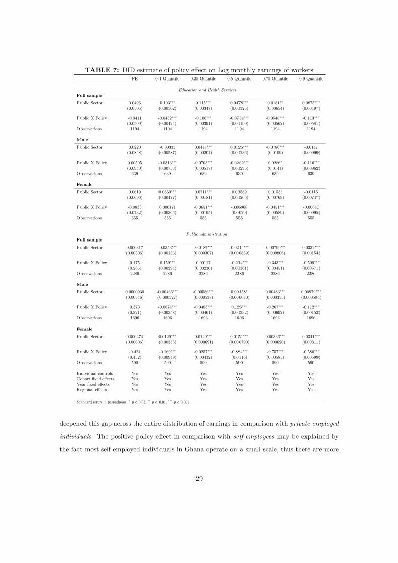
TABLE 7: DID estimate of policy effect on Log monthly earnings of workersFE 0.1 Quantile 0.25 Quantile 0.5 Quantile 0.75 Quantile 0.9 Quantile
Education and Health ServicesFull sample
Public Sector 0.0496 0.103∗∗∗ 0.115∗∗∗ 0.0478∗∗∗ 0.0181∗∗ 0.0875∗∗∗
(0.0505) (0.00502) (0.00347) (0.00325) (0.00654) (0.00497)
Public X Policy -0.0411 -0.0452∗∗∗ -0.106∗∗∗ -0.0754∗∗∗ -0.0548∗∗∗ -0.113∗∗∗
(0.0509) (0.00424) (0.00391) (0.00190) (0.00562) (0.00581)Observations 1194 1194 1194 1194 1194 1194
Male
Public Sector 0.0220 -0.00333 0.0444∗∗∗ 0.0125∗∗∗ -0.0786∗∗∗ -0.0147(0.0848) (0.00587) (0.00204) (0.00236) (0.0109) (0.00999)
Public X Policy 0.00505 -0.0313∗∗∗ -0.0703∗∗∗ -0.0262∗∗∗ 0.0286∗ -0.116∗∗∗
(0.0940) (0.00733) (0.00517) (0.00295) (0.0141) (0.00962)Observations 639 639 639 639 639 639
Female
Public Sector 0.0619 0.0660∗∗∗ 0.0711∗∗∗ 0.03589 0.0153∗ -0.0115(0.0696) (0.00477) (0.00181) (0.00266) (0.00769) (0.00747)
Public X Policy -0.0833 0.000171 -0.0651∗∗∗ -0.06968 -0.0451∗∗∗ -0.00640(0.0732) (0.00366) (0.00195) (0.0029) (0.00589) (0.00995)
Observations 555 555 555 555 555 555
Public administrationFull sample
Public Sector 0.000317 -0.0353∗∗∗ -0.0187∗∗∗ -0.0214∗∗∗ -0.00799∗∗∗ 0.0332∗∗∗
(0.00306) (0.00133) (0.000307) (0.000839) (0.000806) (0.00154)
Public X Policy 0.175 0.159∗∗∗ 0.00117 -0.214∗∗∗ -0.343∗∗∗ -0.509∗∗∗
(0.285) (0.00294) (0.00230) (0.00361) (0.00451) (0.00571)Observations 2286 2286 2286 2286 2286 2286
Male
Public Sector 0.0000930 -0.00466∗∗∗ -0.00586∗∗∗ 0.00158∗ 0.00483∗∗∗ 0.00979∗∗∗
(0.00346) (0.000327) (0.000538) (0.000680) (0.000353) (0.000504)
Public X Policy 0.373 -0.0874∗∗∗ -0.0485∗∗∗ 0.125∗∗∗ -0.267∗∗∗ -0.112∗∗∗
(0.321) (0.00358) (0.00461) (0.00332) (0.00692) (0.00152)Observations 1696 1696 1696 1696 1696 1696
Female
Public Sector 0.000274 0.0129∗∗∗ 0.0120∗∗∗ 0.0151∗∗∗ 0.00336∗∗∗ 0.0341∗∗∗
(0.00606) (0.00355) (0.000691) (0.000790) (0.000620) (0.00311)
Public X Policy -0.424 -0.169∗∗∗ -0.0257∗∗∗ -0.884∗∗∗ -0.757∗∗∗ -0.580∗∗∗
(0.432) (0.00949) (0.00432) (0.0116) (0.00585) (0.00599)Observations 590 590 590 590 590 590
Individual controls Yes Yes Yes Yes Yes YesCohort fixed effects Yes Yes Yes Yes Yes YesYear fixed effects Yes Yes Yes Yes Yes YesRegional effects Yes Yes Yes Yes Yes Yes
Standard errors in parentheses. ∗ p < 0.05, ∗∗ p < 0.01, ∗∗∗ p < 0.001
deepened this gap across the entire distribution of earnings in comparison with private employed
individuals. The positive policy effect in comparison with self-employees may be explained by
the fact most self employed individuals in Ghana operate on a small scale, thus there are more
29
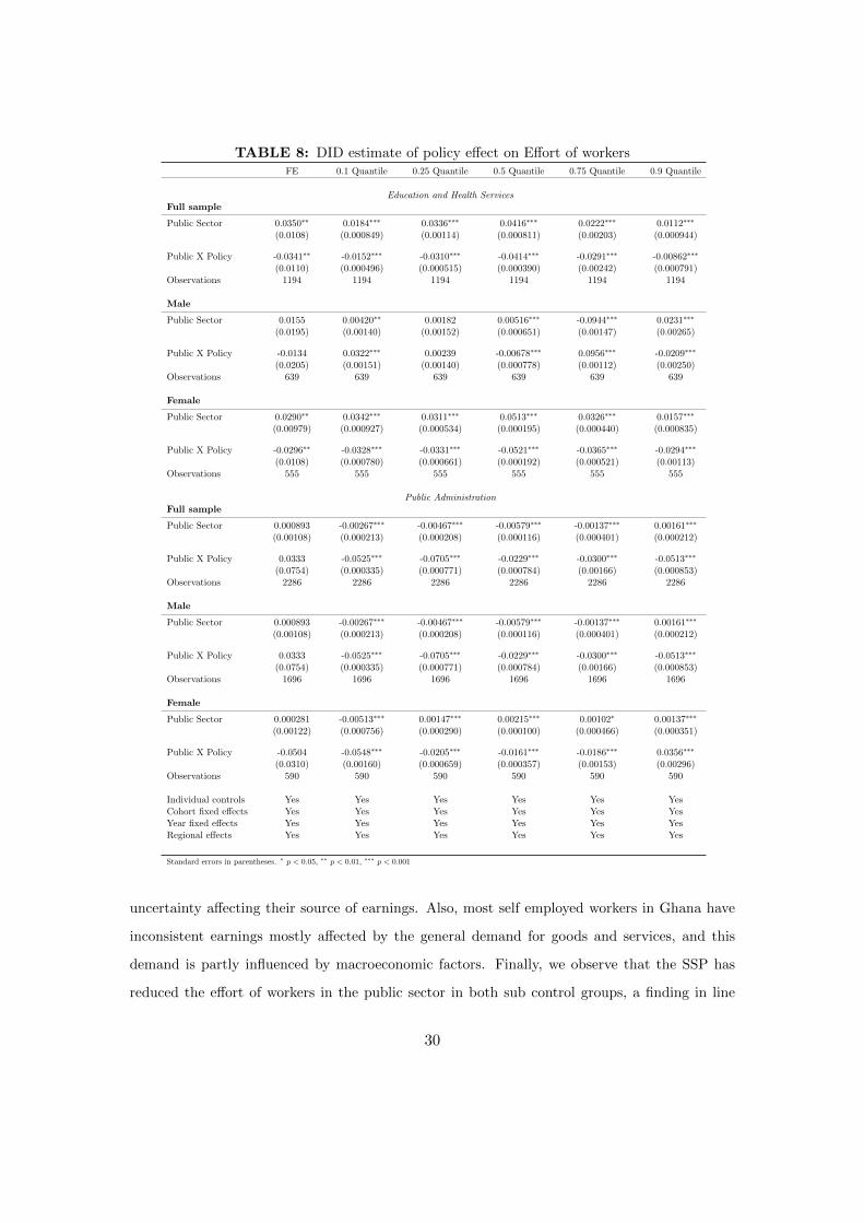
TABLE 8: DID estimate of policy effect on Effort of workersFE 0.1 Quantile 0.25 Quantile 0.5 Quantile 0.75 Quantile 0.9 Quantile
Education and Health ServicesFull sample
Public Sector 0.0350∗∗ 0.0184∗∗∗ 0.0336∗∗∗ 0.0416∗∗∗ 0.0222∗∗∗ 0.0112∗∗∗
(0.0108) (0.000849) (0.00114) (0.000811) (0.00203) (0.000944)
Public X Policy -0.0341∗∗ -0.0152∗∗∗ -0.0310∗∗∗ -0.0414∗∗∗ -0.0291∗∗∗ -0.00862∗∗∗
(0.0110) (0.000496) (0.000515) (0.000390) (0.00242) (0.000791)Observations 1194 1194 1194 1194 1194 1194
Male
Public Sector 0.0155 0.00420∗∗ 0.00182 0.00516∗∗∗ -0.0944∗∗∗ 0.0231∗∗∗
(0.0195) (0.00140) (0.00152) (0.000651) (0.00147) (0.00265)
Public X Policy -0.0134 0.0322∗∗∗ 0.00239 -0.00678∗∗∗ 0.0956∗∗∗ -0.0209∗∗∗
(0.0205) (0.00151) (0.00140) (0.000778) (0.00112) (0.00250)Observations 639 639 639 639 639 639
Female
Public Sector 0.0290∗∗ 0.0342∗∗∗ 0.0311∗∗∗ 0.0513∗∗∗ 0.0326∗∗∗ 0.0157∗∗∗
(0.00979) (0.000927) (0.000534) (0.000195) (0.000440) (0.000835)
Public X Policy -0.0296∗∗ -0.0328∗∗∗ -0.0331∗∗∗ -0.0521∗∗∗ -0.0365∗∗∗ -0.0294∗∗∗
(0.0108) (0.000780) (0.000661) (0.000192) (0.000521) (0.00113)Observations 555 555 555 555 555 555
Public AdministrationFull sample
Public Sector 0.000893 -0.00267∗∗∗ -0.00467∗∗∗ -0.00579∗∗∗ -0.00137∗∗∗ 0.00161∗∗∗
(0.00108) (0.000213) (0.000208) (0.000116) (0.000401) (0.000212)
Public X Policy 0.0333 -0.0525∗∗∗ -0.0705∗∗∗ -0.0229∗∗∗ -0.0300∗∗∗ -0.0513∗∗∗
(0.0754) (0.000335) (0.000771) (0.000784) (0.00166) (0.000853)Observations 2286 2286 2286 2286 2286 2286
Male
Public Sector 0.000893 -0.00267∗∗∗ -0.00467∗∗∗ -0.00579∗∗∗ -0.00137∗∗∗ 0.00161∗∗∗
(0.00108) (0.000213) (0.000208) (0.000116) (0.000401) (0.000212)
Public X Policy 0.0333 -0.0525∗∗∗ -0.0705∗∗∗ -0.0229∗∗∗ -0.0300∗∗∗ -0.0513∗∗∗
(0.0754) (0.000335) (0.000771) (0.000784) (0.00166) (0.000853)Observations 1696 1696 1696 1696 1696 1696
Female
Public Sector 0.000281 -0.00513∗∗∗ 0.00147∗∗∗ 0.00215∗∗∗ 0.00102∗ 0.00137∗∗∗
(0.00122) (0.000756) (0.000290) (0.000100) (0.000466) (0.000351)
Public X Policy -0.0504 -0.0548∗∗∗ -0.0205∗∗∗ -0.0161∗∗∗ -0.0186∗∗∗ 0.0356∗∗∗
(0.0310) (0.00160) (0.000659) (0.000357) (0.00153) (0.00296)Observations 590 590 590 590 590 590
Individual controls Yes Yes Yes Yes Yes YesCohort fixed effects Yes Yes Yes Yes Yes YesYear fixed effects Yes Yes Yes Yes Yes YesRegional effects Yes Yes Yes Yes Yes Yes
Standard errors in parentheses. ∗ p < 0.05, ∗∗ p < 0.01, ∗∗∗ p < 0.001
uncertainty affecting their source of earnings. Also, most self employed workers in Ghana have
inconsistent earnings mostly affected by the general demand for goods and services, and this
demand is partly influenced by macroeconomic factors. Finally, we observe that the SSP has
reduced the effort of workers in the public sector in both sub control groups, a finding in line
30

with our previous analysis.
TABLE 9: DID estimate of policy effect with different control groupsFE 0.1 Quantile 0.25 Quantile 0.5 Quantile 0.75 Quantile 0.9 Quantile
Self-employeesLog of monthly earnings
Public Sector 0.268∗∗∗ 0.0158∗∗∗ 0.0653∗∗∗ 0.150∗∗∗ 0.281∗∗∗ 0.726∗∗∗
(0.0441) (0.000555) (0.000439) (0.000631) (0.00122) (0.00147)
Public X Policy -0.226∗ -0.00290 -0.0145∗∗ 0.0453∗∗∗ -0.0144∗∗ -0.575∗∗∗
(0.0891) (0.00328) (0.00460) (0.00265) (0.00539) (0.00567)
Effort
Public Sector 0.0130∗ 0.000611∗∗∗ -0.00140∗∗∗ 0.00260∗∗∗ 0.0156∗∗∗ 0.0268∗∗∗
(0.00595) (0.000100) (0.000100) (0.000141) (0.000205) (0.000435)
Public X Policy -0.0257 0.0132∗∗∗ -0.00668∗∗∗ -0.00820∗∗∗ -0.0121∗∗∗ -0.0310∗∗∗
(0.0139) (0.000421) (0.000591) (0.000371) (0.00308) (0.00189)
Individual controls Yes Yes Yes Yes Yes YesCohort fixed effects Yes Yes Yes Yes Yes YesYear fixed effects Yes Yes Yes Yes Yes YesRegional effects Yes Yes Yes Yes Yes YesObservations 7284 7284 7284 7284 7284 7284
Private employed individualsLog of monthly earnings
Public Sector -0.511∗∗∗ -0.120∗∗∗ -0.252∗∗∗ -0.893∗∗∗ -1.218∗∗∗ -0.929∗∗∗
(0.0567) (0.00121) (0.000429) (0.000485) (0.00161) (0.00120)
Public X Policy 0.475∗∗∗ 0.0483∗∗∗ 0.175∗∗∗ 0.827∗∗∗ 1.125∗∗∗ 0.794∗∗∗
(0.0535) (0.00197) (0.00120) (0.000596) (0.00212) (0.00113)
Effort
Public sector 0.00893 -0.0319∗∗∗ -0.0269∗∗∗ -0.0404∗∗∗ -0.0356∗∗∗ -0.111∗∗∗
(0.00697) (0.000142) (0.0000412) (0.0000897) (0.0000535) (0.000311)
Public X Policy -0.0139 0.0289∗∗∗ 0.0199∗∗∗ 0.0358∗∗∗ 0.0347∗∗∗ 0.117∗∗∗
(0.00801) (0.000263) (0.000130) (0.0000482) (0.0000921) (0.000362)
Individual controls Yes Yes Yes Yes Yes YesCohort fixed effects Yes Yes Yes Yes Yes YesYear fixed effects Yes Yes Yes Yes Yes YesRegional effects Yes Yes Yes Yes Yes YesObservations 8772 8772 8772 8772 8772 8772
Standard errors in parentheses. ∗ p < 0.05, ∗∗ p < 0.01, ∗∗∗ p < 0.001
31
VI Robustness Checks
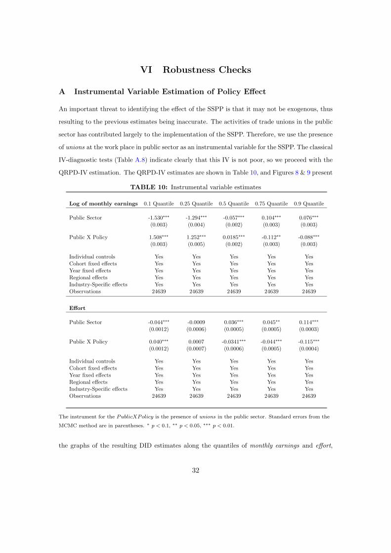
A Instrumental Variable Estimation of Policy Effect
An important threat to identifying the effect of the SSPP is that it may not be exogenous, thus
resulting to the previous estimates being inaccurate. The activities of trade unions in the public
sector has contributed largely to the implementation of the SSPP. Therefore, we use the presence
of unions at the work place in public sector as an instrumental variable for the SSPP. The classical
IV-diagnostic tests (Table A.8) indicate clearly that this IV is not poor, so we proceed with the
QRPD-IV estimation. The QRPD-IV estimates are shown in Table 10, and Figures 8 & 9 present
TABLE 10: Instrumental variable estimates
Log of monthly earnings 0.1 Quantile 0.25 Quantile 0.5 Quantile 0.75 Quantile 0.9 Quantile
Public Sector -1.530∗∗∗ -1.294∗∗∗ -0.057∗∗∗ 0.104∗∗∗ 0.076∗∗∗
(0.003) (0.004) (0.002) (0.003) (0.003)
Public X Policy 1.508∗∗∗ 1.252∗∗∗ 0.0185∗∗∗ -0.112∗∗ -0.088∗∗∗
(0.003) (0.005) (0.002) (0.003) (0.003)
Individual controls Yes Yes Yes Yes YesCohort fixed effects Yes Yes Yes Yes YesYear fixed effects Yes Yes Yes Yes YesRegional effects Yes Yes Yes Yes YesIndustry-Specific effects Yes Yes Yes Yes YesObservations 24639 24639 24639 24639 24639
Effort
Public Sector -0.044∗∗∗ -0.0009 0.036∗∗∗ 0.045∗∗ 0.114∗∗∗
(0.0012) (0.0006) (0.0005) (0.0005) (0.0003)
Public X Policy 0.040∗∗∗ 0.0007 -0.0341∗∗∗ -0.044∗∗∗ -0.115∗∗∗
(0.0012) (0.0007) (0.0006) (0.0005) (0.0004)
Individual controls Yes Yes Yes Yes YesCohort fixed effects Yes Yes Yes Yes YesYear fixed effects Yes Yes Yes Yes YesRegional effects Yes Yes Yes Yes YesIndustry-Specific effects Yes Yes Yes Yes YesObservations 24639 24639 24639 24639 24639
The instrument for the PublicXPolicy is the presence of unions in the public sector. Standard errors from the
MCMC method are in parentheses. ∗ p < 0.1, ∗∗ p < 0.05, ∗∗∗ p < 0.01.
the graphs of the resulting DID estimates along the quantiles of monthly earnings and effort,
32

both the full sample [Subfigures (a)] and the subsamples of males and females [Subfigures (b)].
The results align qualitatively with our previous analysis in Section V. Quantitatively, the SSPP
has a smaller effect on monthly earnings at higher tail of the distribution compared with the
results of Section V. Regarding effort, the difference between the QRPD-IV estimates in Figure
9 and that of the standard QRPD estimates in Section II are quite similar.
FIGURE 8: DID estimates of the SSPP effect on monthly earnings
(a) Full sample (b) Males vs. Females
FIGURE 9: DID estimates of the SSPP effect on effort
(a) Full sample (b) Males vs. Females
B Placebo Tests and Other Robustness Checks
The identification of the policy effect depends on the validity of the underlying assumptions.
One of this assumption is that there are no confounding factors other then the SSPP that could
33
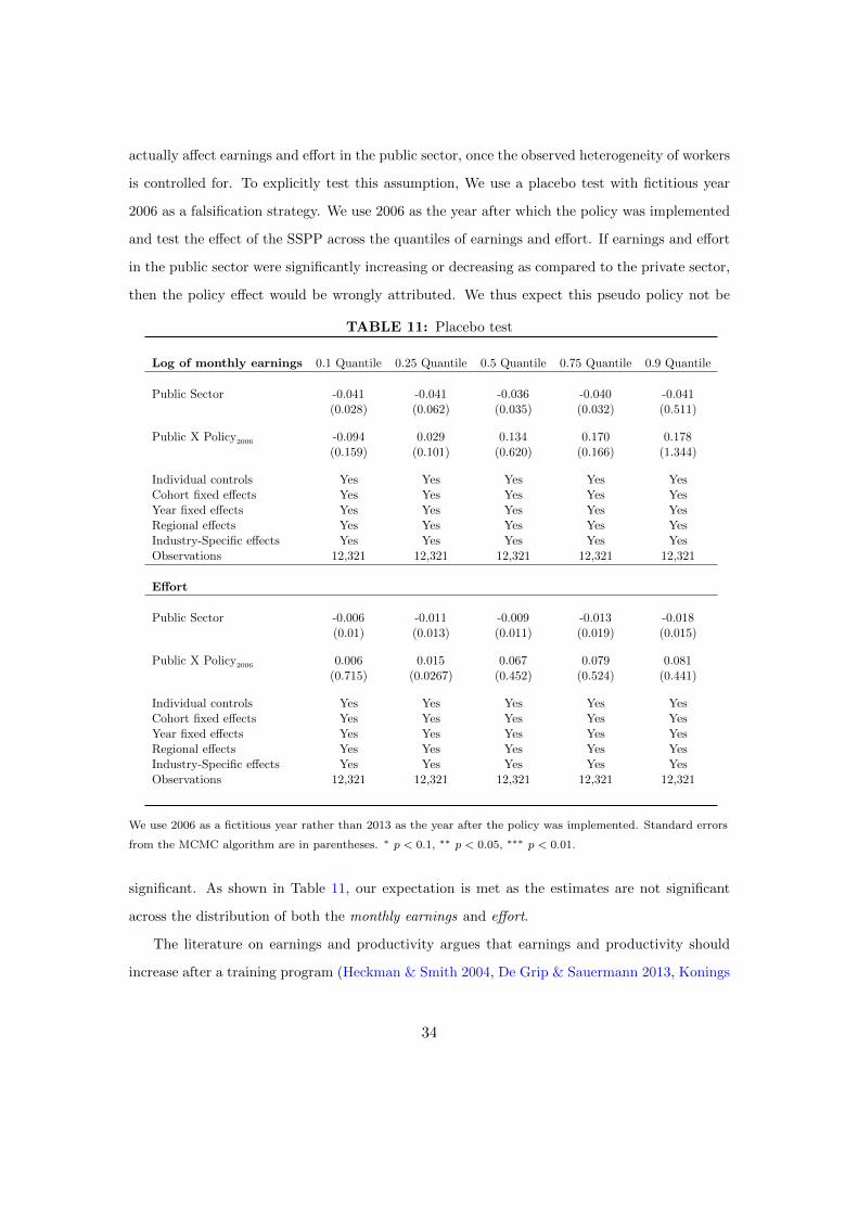
actually affect earnings and effort in the public sector, once the observed heterogeneity of workers
is controlled for. To explicitly test this assumption, We use a placebo test with fictitious year
2006 as a falsification strategy. We use 2006 as the year after which the policy was implemented
and test the effect of the SSPP across the quantiles of earnings and effort. If earnings and effort
in the public sector were significantly increasing or decreasing as compared to the private sector,
then the policy effect would be wrongly attributed. We thus expect this pseudo policy not be
TABLE 11: Placebo test
Log of monthly earnings 0.1 Quantile 0.25 Quantile 0.5 Quantile 0.75 Quantile 0.9 Quantile
Public Sector -0.041 -0.041 -0.036 -0.040 -0.041(0.028) (0.062) (0.035) (0.032) (0.511)
Public X Policy2006 -0.094 0.029 0.134 0.170 0.178(0.159) (0.101) (0.620) (0.166) (1.344)
Individual controls Yes Yes Yes Yes YesCohort fixed effects Yes Yes Yes Yes YesYear fixed effects Yes Yes Yes Yes YesRegional effects Yes Yes Yes Yes YesIndustry-Specific effects Yes Yes Yes Yes YesObservations 12,321 12,321 12,321 12,321 12,321
Effort
Public Sector -0.006 -0.011 -0.009 -0.013 -0.018(0.01) (0.013) (0.011) (0.019) (0.015)
Public X Policy2006 0.006 0.015 0.067 0.079 0.081(0.715) (0.0267) (0.452) (0.524) (0.441)
Individual controls Yes Yes Yes Yes YesCohort fixed effects Yes Yes Yes Yes YesYear fixed effects Yes Yes Yes Yes YesRegional effects Yes Yes Yes Yes YesIndustry-Specific effects Yes Yes Yes Yes YesObservations 12,321 12,321 12,321 12,321 12,321
We use 2006 as a fictitious year rather than 2013 as the year after the policy was implemented. Standard errors
from the MCMC algorithm are in parentheses. ∗ p < 0.1, ∗∗ p < 0.05, ∗∗∗ p < 0.01.
significant. As shown in Table 11, our expectation is met as the estimates are not significant
across the distribution of both the monthly earnings and effort.
The literature on earnings and productivity argues that earnings and productivity should
increase after a training program (Heckman & Smith 2004, De Grip & Sauermann 2013, Konings
34
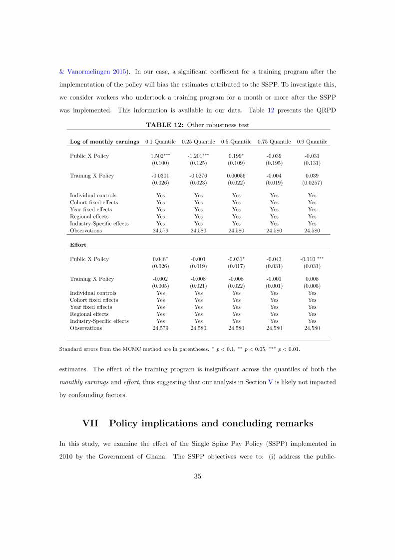
& Vanormelingen 2015). In our case, a significant coefficient for a training program after the
implementation of the policy will bias the estimates attributed to the SSPP. To investigate this,
we consider workers who undertook a training program for a month or more after the SSPP
was implemented. This information is available in our data. Table 12 presents the QRPD
TABLE 12: Other robustness test
Log of monthly earnings 0.1 Quantile 0.25 Quantile 0.5 Quantile 0.75 Quantile 0.9 Quantile
Public X Policy 1.502∗∗∗ -1.201∗∗∗ 0.199∗ -0.039 -0.031(0.100) (0.125) (0.109) (0.195) (0.131)
Training X Policy -0.0301 -0.0276 0.00056 -0.004 0.039(0.026) (0.023) (0.022) (0.019) (0.0257)
Individual controls Yes Yes Yes Yes YesCohort fixed effects Yes Yes Yes Yes YesYear fixed effects Yes Yes Yes Yes YesRegional effects Yes Yes Yes Yes YesIndustry-Specific effects Yes Yes Yes Yes YesObservations 24,579 24,580 24,580 24,580 24,580
Effort
Public X Policy 0.048∗ -0.001 -0.031∗ -0.043 -0.110 ∗∗∗
(0.026) (0.019) (0.017) (0.031) (0.031)
Training X Policy -0.002 -0.008 -0.008 -0.001 0.008(0.005) (0.021) (0.022) (0.001) (0.005)
Individual controls Yes Yes Yes Yes YesCohort fixed effects Yes Yes Yes Yes YesYear fixed effects Yes Yes Yes Yes YesRegional effects Yes Yes Yes Yes YesIndustry-Specific effects Yes Yes Yes Yes YesObservations 24,579 24,580 24,580 24,580 24,580
Standard errors from the MCMC method are in parentheses. ∗ p < 0.1, ∗∗ p < 0.05, ∗∗∗ p < 0.01.
estimates. The effect of the training program is insignificant across the quantiles of both the
monthly earnings and effort, thus suggesting that our analysis in Section V is likely not impacted
by confounding factors.
VII Policy implications and concluding remarks
In this study, we examine the effect of the Single Spine Pay Policy (SSPP) implemented in
2010 by the Government of Ghana. The SSPP objectives were to: (i) address the public-
35
private wage gap, and (ii) increase the productivity in the public sector. Using a quantile
treatment effect approach based on a Difference-In-Difference (DID) estimation, we show that
the SSPP has yet to reduce the public-private sector pay differentials across the whole distri-
bution of earnings in Ghana. The improvement observed is mostly at the lower tail of the
distribution of earnings. Nevertheless, the SSPP was successful in reducing the gender-wage gap
in the education and health services sector, but the policy has also decreased the productivity
of workers, mainly due to a decrease in the effort of males workers in the public sector. Our
findings are supported by a number of robustness checks, and the quantile approach adopted
shows that examining a policy effect at the averages may not always be the appropriate way as
noted by Firpo (2007).
The reduction in the effort after the implementation of the policy, especially by female
workers in the public sector, requires more attention. Indeed, females public sector workers have
seen a major reduction in their hours of work after 2010. The backward bending nature of their
supply curve is mostly seen beyond the 25th quantile of the distribution of hours of work. Our
understanding of this phenomena is that most females in the public sector with hours of work
beyond the 25th quantile are married and have children. The young and unmarried women are
mostly those willing to spend 8 hours a day at work, as they have less family responsibilities.
For example, Heath (2017) found in urban Ghana that women are likely to reduce their hours
of work when they have children, except if they are self-employed. Another factor that could
also explain the fall in effort in the public sector is the increasing number of strikes after the
implementation of the SSPP. Most public sector workers were critical of this policy, and this was
accentuated by their increase participation in unions’activities.
Furthermore, the discrepancies associated with late payments of wages and the possibility
that some workers will not be paid in full, has resulted in a far more severe strikes in the public
sector. This late payments mostly stem from the inconsistencies in the rents from the oil sale.
As shown in Figure 1c, the fall in the contribution of oil rents to total GDP along with the
over-dependence on the gains from a volatile source have introduced a lot of uncertainties in the
pay of public sector workers. This volatile nature of the oil rents raises the question of whether
the SSPP can be sustained. It is fair to say that the ability of the Government to sustain this
policy will largely depend on how it cautiously manages its expenditure, and more importantly
36
the allocation of its resources towards more diverse productive areas.
Other macroeconomic factors have impacted the success of the SSPP. In particular, the
continuous rise in inflation and daily depreciation of the local currency do not align with a
policy that is revised only at the end of a calendar year. In the private sector, most firms have
policies or measures that facilitate the revision of wages within a year to account for changing
environment and living costs. This is quasi-nonexistent in the public sector, which does not
favor a policy like the SSPP to have its desired impact. Nevertheless, the SSPP has had some
successes. In particular, this policy has reduced the gender-wage gap in the education and
health services sector, and it could be improved by putting in place a good managerial quality
in the government’ agencies. Also, our econometric analysis of the effect of this policy has some
challenges. For example, the availability of data does not make it possible to measure the effect
of the policy over a longer time period. We hope that future research could be done in that
perspective once data become available.
References
Adamchik, V. A. & Bedi, A. S. (2000), ‘Wage differentials between the public and the private
sectors: Evidence from an economy in transition’, Labour economics 7(2), 203–224.
Aizer, A. (2010), ‘The gender wage gap and domestic violence’, The American economic review
100(4), 1847.
Akerlof, G. A. (1982), ‘Labor contracts as partial gift exchange’, The quarterly journal of eco-
nomics 97(4), 543–569.
Akerlof, G. A. (1984), ‘Gift exchange and efficiency-wage theory: Four views’, The American
Economic Review 74(2), 79–83.
Akerlof, G. A. & Yellen, J. L. (1990), ‘The fair wage-effort hypothesis and unemployment’, The
Quarterly Journal of Economics 105(2), 255–283.
Alexopoulos, M. (2002), ‘Shirking in a monetary business cycle model’, The Canadian Journal
of Economics / Revue canadienne d’Economique 39(3), 689–718.
37

Baah, A. Y. & Reilly, B. (2009), ‘An empirical analysis of strike durations in Ghana from 1980
to 2004’, Labour 23(3), 459–479.
Bajorek, Z. M. & Bevan, S. M. (2015), ‘Performance-related-pay in the UK public sector: A
review of the recent evidence on effectiveness and value for money’, Journal of Organizational
Effectiveness: People and Performance 2(2), 94–109.
Besley, T. & Case, A. (2000), ‘Unnatural experiments? Estimating the incidence of endogenous
policies’, The Economic Journal 110(467), 672–694.
Bregn, K. (2013), ‘Detrimental effects of performance-related pay in the public sector? On the
need for a broader theoretical perspective’, Public Organization Review 13(1), 21–35.
Bryson, A., Freeman, R., Lucifora, C., Pellizzari, M., Perotin, V. et al. (2012), Paying for
performance: Incentive pay schemes and employees’ financial participation, Technical report,
Centre for Economic Performance, LSE.
Campbell, C. M. (2006), ‘A model of the determinants of effort’, Economic Modelling 23(2), 215–
237.
Cohen, P. N. & Huffman, M. L. (2007), ‘Working for the woman? Female managers and the
gender wage gap’, American Sociological Review 72(5), 681–704.
Damiani, M., Pompei, F. & Ricci, A. (2016), ‘Performance related pay, productivity and wages
in Italy: A quantile regression approach’, International Journal of Manpower 37(2), 344–371.
De Grip, A. & Sauermann, J. (2013), ‘The effect of training on productivity: The transfer of
on-the-job training from the perspective of economics’, Educational Research Review 8, 28–36.
Deaton, A. (1985), ‘Panel data from time series of cross-sections’, Journal of econometrics 30(1-
2), 109–126.
Easterly, W. & Levine, R. (1997), ‘Africa’s growth tragedy: Policies and ethnic divisions’, The
Quarterly Journal of Economics 112(4), 1203–1250.
Firpo, S. (2007), ‘Efficient semiparametric estimation of quantile treatment effects’, Econometrica
75(1), 259–276.
38
Frey, B. S. (1993), ‘Shirking or work morale?: The impact of regulating’, European Economic
Review 37(8), 1523–1532.
FWSC (2009), Government white paper on the Single Spine Pay Policy, Technical report, Gov-
ernment of Ghana.
Ghana Statistical Service (2016), ‘Ghana living standards survey main report’. http://www.
statsghana.gov.gh/nada/index.php/catalog/72.
Glewwe, P. (1991), Schooling, skills, and the returns to government investment in education:
An exploration using data from Ghana. Living standards measurement study, working paper
No.76, ERIC.
Hasnain, Z. & Pierskalla, H. N. (2012), ‘Performance-related pay in the public sector: A review
of theory and evidence’, World Bank Policy Research .
Heath, R. (2017), ‘Fertility at work: Children and women’s labor market outcomes in urban
Ghana’, Journal of Development Economics 126, 190–214.
Heckman, J. J. & Smith, J. A. (2004), ‘The determinants of participation in a social program:
Evidence from a prototypical job training program’, Journal of Labor Economics 22(2), 243–
298.
Heyes, A. (2005), ‘The economics of vocation or ‘why is a badly paid nurse a good nurse’?’,
Journal of Health Economics 24(3), 561–569.
Katz, L. F. (1986), ‘Efficiency wage theories: A partial evaluation’, NBER macroeconomics
annual 1, 235–276.
Koenker, R. & Bassett Jr, G. (1978), ‘Regression quantiles’, Econometrica 46(1), 33–50.
Konings, J. & Vanormelingen, S. (2015), ‘The impact of training on productivity and wages:
firm-level evidence’, Review of Economics and Statistics 97(2), 485–497.
Lausev, J. (2014), ‘What has 20 years of public–private pay gap literature told us? eastern
european transitioning vs. developed economies’, Journal of Economic Surveys 28(3), 516–
550.
39
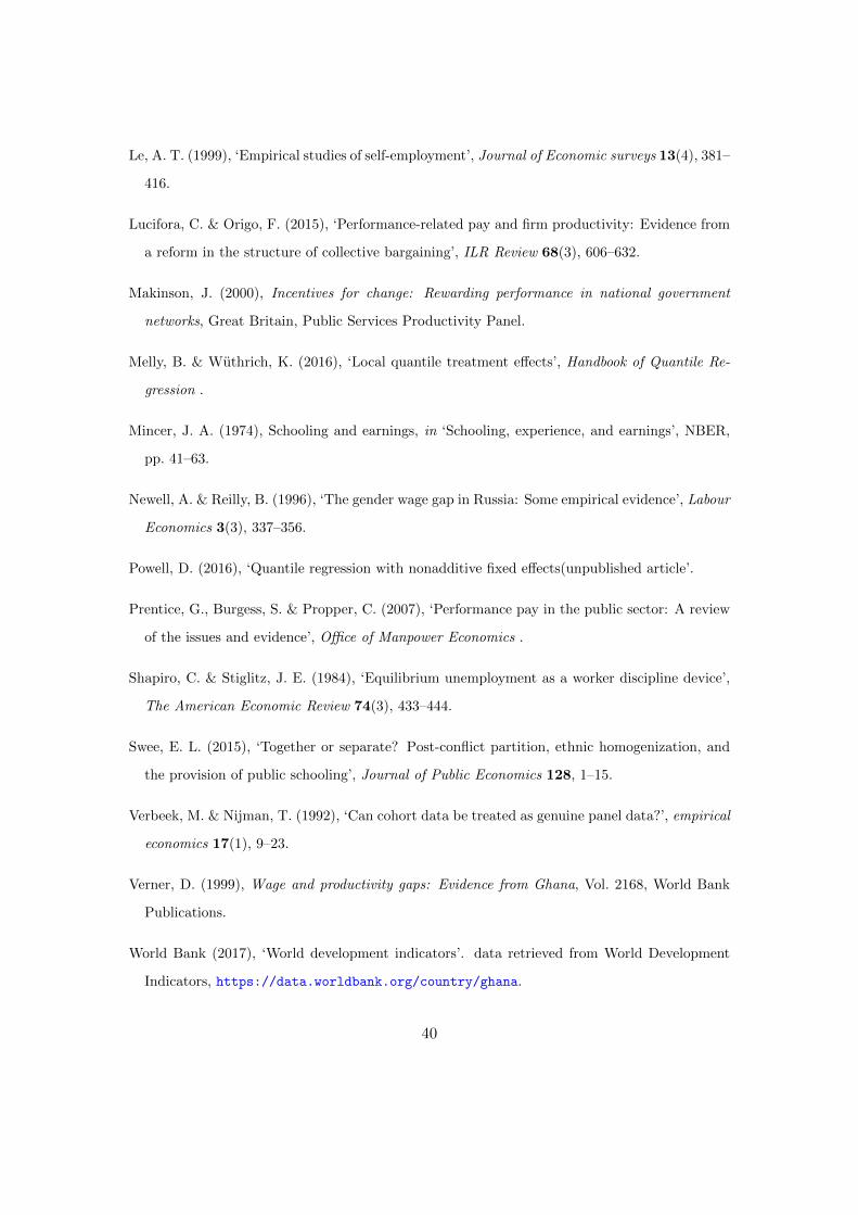
Le, A. T. (1999), ‘Empirical studies of self-employment’, Journal of Economic surveys 13(4), 381–
416.
Lucifora, C. & Origo, F. (2015), ‘Performance-related pay and firm productivity: Evidence from
a reform in the structure of collective bargaining’, ILR Review 68(3), 606–632.
Makinson, J. (2000), Incentives for change: Rewarding performance in national government
networks, Great Britain, Public Services Productivity Panel.
Melly, B. & Wuthrich, K. (2016), ‘Local quantile treatment effects’, Handbook of Quantile Re-
gression .
Mincer, J. A. (1974), Schooling and earnings, in ‘Schooling, experience, and earnings’, NBER,
pp. 41–63.
Newell, A. & Reilly, B. (1996), ‘The gender wage gap in Russia: Some empirical evidence’, Labour
Economics 3(3), 337–356.
Powell, D. (2016), ‘Quantile regression with nonadditive fixed effects(unpublished article’.
Prentice, G., Burgess, S. & Propper, C. (2007), ‘Performance pay in the public sector: A review
of the issues and evidence’, Office of Manpower Economics .
Shapiro, C. & Stiglitz, J. E. (1984), ‘Equilibrium unemployment as a worker discipline device’,
The American Economic Review 74(3), 433–444.
Swee, E. L. (2015), ‘Together or separate? Post-conflict partition, ethnic homogenization, and
the provision of public schooling’, Journal of Public Economics 128, 1–15.
Verbeek, M. & Nijman, T. (1992), ‘Can cohort data be treated as genuine panel data?’, empirical
economics 17(1), 9–23.
Verner, D. (1999), Wage and productivity gaps: Evidence from Ghana, Vol. 2168, World Bank
Publications.
World Bank (2017), ‘World development indicators’. data retrieved from World Development
Indicators, https://data.worldbank.org/country/ghana.
40

A Appendix
A Construction of pseudo panels
TABLE A.1: Survey years
Year Frequency Percentage
1998 5,433 22.052006 6,888 27.962013 12,318 49.99
Total 24,639 100.00
TABLE A.2: Respondents by gender
Year Frequency Percentage
Males 13,774 55.90Females 10,865 44.10
Total 24,639 100.00
TABLE A.3: Year cohorts
Year Cohorts Frequency Percentage
1930-1955 4,001 16.241956-1962 3,772 15.311963-1968 4,156 16.871969-1975 4,176 16.951976-1982 4,197 17.031983-1999 4,337 17.60
Total 24,639 100.00
TABLE A.4: Ethnic cohorts
Year Cohorts Frequency Percentage
Akan 13,589 55.15Ga-Dangme 2,309 9.37Ewe 3,916 15.89Guan 1,203 4.88Dagbani 1,876 7.61Others1 1,746 7.09
Total 24,639 100.00
41

FIGURE A.1
TABLE A.5: Descriptive statisticsBefore Policy After Policy
Total Private Sector Public Sector Diff(Pr-Pu) Total Private Sector Public Sector Diff(Pr-Pu)
Log of Monthly Income 3.907∗∗∗ 4.066∗∗∗ 3.747∗∗∗ 6.217∗∗∗ 6.210∗∗∗ 6.274∗∗∗ ∗∗∗
(0.061) (0.009) (0.114) (0.003) (0.003) (0.011)
Log of Hours of Work 3.807∗∗∗ 3.816∗∗∗ 3.798∗∗∗ 4.786∗∗∗ 4.785∗∗∗ 4.796∗∗∗ ∗∗∗
(0.014) (0.027) (0.001) (0.06) 0.006 (0.002)
Years of Education 7.572∗∗∗ 7.374∗∗∗ 7.769∗∗∗ 7.642∗∗∗ 7.223∗∗∗ 11.641∗∗∗ ∗∗∗
(0.037) (0.023) (0.579) (0.015) 0.012 0.023
Experience 10.602 10.535 10.789 10.741∗∗∗ 10.723∗∗∗ 10.89∗∗∗
(6.176) (6.197) (6.119) (0.096) (0.1023) (0.2782)
Square of Experience/100 1.505 1.494 1.538 2.287∗∗∗ 2.22∗∗∗ 2.29∗∗∗
(1.596) (1.602) (1.581) (0.039) (0.043) (0.107)
Married Workers 0.630 0.545 0.715 0.679∗∗∗ 0.676∗∗∗ 0.703∗∗∗ ∗∗
(0.487) (0.522) (0.451) (0.004) 0.004 0.012
Male Workers 0.556∗∗ 0.538 0.572 0.546∗∗∗ 0.538∗∗∗ 0.615∗∗∗ ∗∗∗
(0.272) (0.519) (0.495) (0.004) (0.005) 0.013
Formally Employed Father 0.192 0.077 0.306 0.404∗∗∗ 0.389∗∗∗ 0.526∗∗∗ ∗∗∗
(0.369) (0.277) (0.461) (0.004) (0.005) (0.014)
Observations 12,321 5,433 6,888 12,318 7,532 4,786
Standard errors in parentheses. ∗ p < 0.1, ∗∗ p < 0.05, ∗∗∗ p < 0.001
42
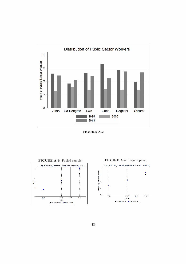
FIGURE A.2
FIGURE A.3: Pooled sample FIGURE A.4: Pseudo panel
43

FIGURE A.5: Pooled sample FIGURE A.6: Pseudo panel
FIGURE A.7: Pooled sample FIGURE A.8: Pseudo panel
FIGURE A.9: Pooled sample FIGURE A.10: Pseudo panel
44
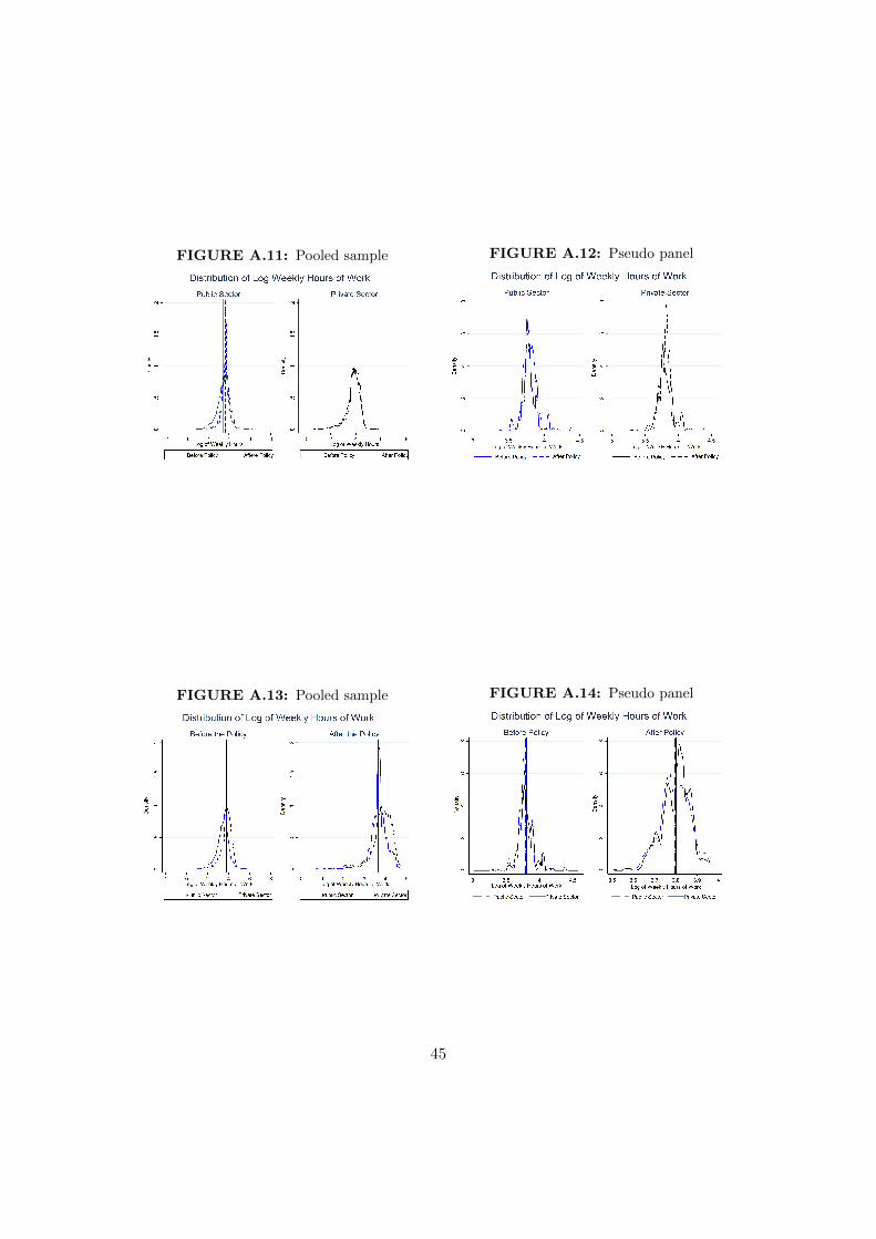
FIGURE A.11: Pooled sample FIGURE A.12: Pseudo panel
FIGURE A.13: Pooled sample FIGURE A.14: Pseudo panel
45
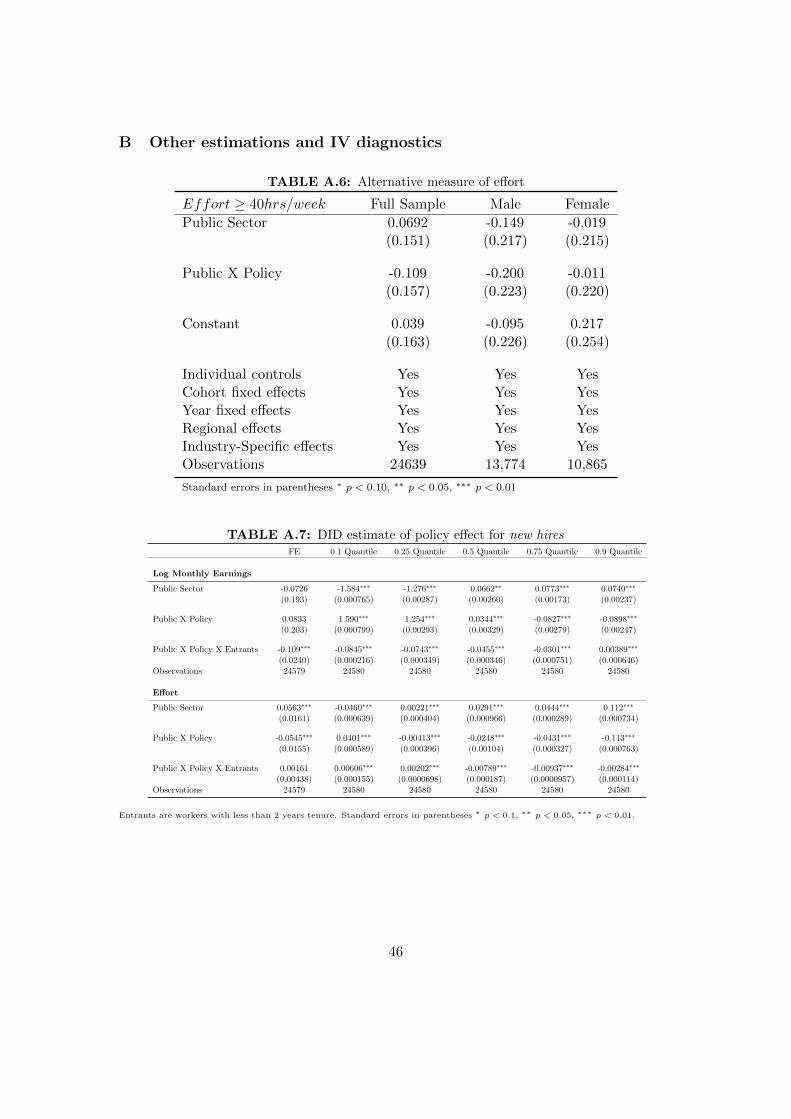
B Other estimations and IV diagnostics
TABLE A.6: Alternative measure of effort
Effort ≥ 40hrs/week Full Sample Male Female
Public Sector 0.0692 -0.149 -0.019(0.151) (0.217) (0.215)
Public X Policy -0.109 -0.200 -0.011(0.157) (0.223) (0.220)
Constant 0.039 -0.095 0.217(0.163) (0.226) (0.254)
Individual controls Yes Yes YesCohort fixed effects Yes Yes YesYear fixed effects Yes Yes YesRegional effects Yes Yes YesIndustry-Specific effects Yes Yes YesObservations 24639 13,774 10,865
Standard errors in parentheses ∗ p < 0.10, ∗∗ p < 0.05, ∗∗∗ p < 0.01
TABLE A.7: DID estimate of policy effect for new hiresFE 0.1 Quantile 0.25 Quantile 0.5 Quantile 0.75 Quantile 0.9 Quantile
Log Monthly Earnings
Public Sector -0.0726 -1.584∗∗∗ -1.276∗∗∗ 0.0662∗∗ 0.0773∗∗∗ 0.0740∗∗∗
(0.193) (0.000765) (0.00287) (0.00260) (0.00173) (0.00237)
Public X Policy 0.0833 1.590∗∗∗ 1.254∗∗∗ 0.0344∗∗∗ -0.0827∗∗∗ -0.0898∗∗∗
(0.203) (0.000799) (0.00293) (0.00329) (0.00279) (0.00247)
Public X Policy X Entrants -0.109∗∗∗ -0.0845∗∗∗ -0.0743∗∗∗ -0.0455∗∗∗ -0.0301∗∗∗ 0.00389∗∗∗
(0.0240) (0.000216) (0.000349) (0.000346) (0.000751) (0.000646)Observations 24579 24580 24580 24580 24580 24580
Effort
Public Sector 0.0563∗∗∗ -0.0460∗∗∗ 0.00221∗∗∗ 0.0291∗∗∗ 0.0444∗∗∗ 0.112∗∗∗
(0.0161) (0.000639) (0.000404) (0.000966) (0.000289) (0.000734)
Public X Policy -0.0545∗∗∗ 0.0401∗∗∗ -0.00413∗∗∗ -0.0248∗∗∗ -0.0431∗∗∗ -0.113∗∗∗
(0.0155) (0.000589) (0.000396) (0.00104) (0.000327) (0.000763)
Public X Policy X Entrants 0.00161 0.00606∗∗∗ 0.00202∗∗∗ -0.00789∗∗∗ -0.00937∗∗∗ -0.00284∗∗∗
(0.00438) (0.000155) (0.0000698) (0.000187) (0.0000957) (0.000114)Observations 24579 24580 24580 24580 24580 24580
Entrants are workers with less than 2 years tenure. Standard errors in parentheses ∗ p < 0.1, ∗∗ p < 0.05, ∗∗∗ p < 0.01.
46
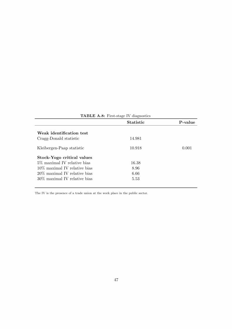
TABLE A.8: First-stage IV diagnostics
Statistic P-value
Weak identification testCragg-Donald statistic 14.981
Kleibergen-Paap statistic 10.918 0.001
Stock-Yogo critical values5% maximal IV relative bias 16.3810% maximal IV relative bias 8.9620% maximal IV relative bias 6.6630% maximal IV relative bias 5.53
The IV is the presence of a trade union at the work place in the public sector.
47