2009 OKSWP0908

Economics Working Paper Series

OKLAHOMA STATE UNIVERSITY

School Feeding Programs and the Nutrition of Siblings:

Evidence from a Randomized Trial in Rural Burkina Faso

Harounan Kazianga Oklahoma State University

Email: harounan.kazianga@okstate.edu

Damien de Walque The World Bank

Email: ddewalque@worldbank.org

Harold Alderman The World Bank

Email: halderman@worldbank.org

Department of Economics Oklahoma S

tate

Stillwater, Oklahoma University

339 BUS, Stillwater, OK 74078, Ph 405-744-5110, Fax 405-744-5180 Harounan Kazianga harounan.kazianga@okstate.edu

Abdul Munasib munasib@okstate.edu

School Feeding Programs and the Nutrition of Siblings:

Evidence from a Randomized Trial in Rural Burkina Faso∗

Harounan Kazianga Damien de Walque Harold Alderman

Oklahoma State University The World Bank The World Bank

harounan.kazianga@okstate.edu ddewalque@worldbank.org halderman@worldbank.org

November, 30 2009

Key Words: School feeding, pre-school age children nutrition, intra-household, randomized trial JEL Codes: H,I,O

∗We thank the World Food Program and the World Bank Research Committee for their financial support. We thank the Ministry of Education of Burkina Faso, and its regional and provincial offices in the Sahel region for supporting and facilitating the roll out of the experiment. We thank Pierre Kamano, Tshiya Subayi and Timothy Johnston from the World Bank and Annalisa Conte, Olga Keita, Kerren Hedlund, Ute Meier, Ali Ouattara and Bernadette Tapsoba from the World Food Program for their support and advice. We thank Jean-Pierre Sawadogo and Yiriyibin Bambio from the University of Ouagadougou and Laeticia Ouedraogo from the Institut de Recherche en Sciences de la Santé for coordinating the field work. We thank seminar participants at the World Bank, at Purdue University, at the University of Oklahoma and at NEUDC for valuable comments. The findings, interpretations and conclusions expressed are entirely those of the authors. They do not necessarily represent the views of the World Bank, its Executive Directors, or the countries they represent, nor do they reflect the views of the World Food Program. 

2

Abstract:

This paper uses a prospective randomized trial to assess the impact of two school feeding schemes on health outcomes for pre-school age children from low-income households in northern rural Burkina Faso. The two school feeding programs under consideration are, on the one hand, school meals where students are provided with lunch each school day, and, on the other hand, take home rations which provide girls with 10 kg of cereal flour each month, conditional on 90 percent attendance rate. A unique feature of this program is that data were collected for both children who were enrolled in school and those who were not, hence allowing a direct measure of the spillover effect on children who are too young to be enrolled. After the program ran for one academic year, we found the following impacts on children age 5 and under: take-home rations have increased weight-for-age by .34 standard deviations for boys and girls taken jointly, and by .57 standard deviations for boys taken separately. The school meals intervention has increased weight-for-age by .40 for boys. Neither program had significant impact on girls taken separately. We show that achieving the same gains through increased household expenditures would have required cash transfers much larger than the monetary value of the food transfers. This indicates that most of the gains are realized through intra-household food reallocation.

Key Words: School feeding, pre-school age children nutrition, intra-household, randomized trial JEL Codes: H,I,O

3

1. Introduction.

School feeding programs are popular transfer programs in both developed countries and

low income settings. There is extensive evidence that these programs increase school enrolment

or attendance in communities where schooling is not universal (Adelman et al., 2008). Their

impact on nutrition is less clear, however, in part because the “window of opportunity” for

nutrition closes long before class room education begins. This reflects the fact that malnutrition

in utero or the first 24 months of life has irreversible lifetime consequences (Shrimpton et al.

2001).

There is also a concern that even when targeted to school aged children such school feeding

programs have only a modest impact on this population since intrahousehold reallocation of

resources can negate the targeting of food resources to students. However, if such a reallocation

were to occur it may, in fact, increase the overall nutritional impact of the feeding program to the

degree that the reallocation is targeted towards more vulnerable members of a household.

Relatively few of the studies of school feeding, however, have included data on the younger

siblings of the student population. For example, a recent comprehensive meta-analysis of

medical and nutritional literature covering various dimensions of school feeding (Kristjansson et

al., 2007) does not address the impact on siblings although it does find an impact on the weights

of direct beneficiaries.

This study addresses the question of the impact of school feeding on the nutritional status of

children not yet in school using a randomized design of a program in Burkina Faso, finding that

two different types of food for education transfers lead to increased weight for age of these

younger children. We use an experimental, prospective randomized design in which villages are

4

randomly assigned to treatment and control groups and data are collected before the interventions

are rolled out and after the interventions have been implemented (Burges, 1995; Duflo,

Glennerster and Kremer, 2008). There are two benefits to our research design. First, unlike

many studies, we cover both children who are in an out of school. Second, and more importantly,

our measure of nutritional status covers children who are too young to be enrolled (0 to 60

months). Hence, the design provides a direct measure of spillover effects.

2. Background on School Feeding and Nutrition

Food for education programs may be in the form of school meals and snacks or as take home

rations (THR). The former are seldom targeted within a school (although in some program there

is a fee which may vary by individuals). In partial contrast, THR can provide a transfer that is

targeted to some students but not others. In neither case is the increment to the child’s diet

necessarily identical to the food transfer. Even in the case of meals consumed in the school meal

or similar food supplement, the child may reduce his or her consumption of foods that would

have been consumed in the absence of the school meal outside the school (Beaton and Ghassemi,

1982).1 Similarly, the impact of THR on the child’s food intake depends on intrahousehold

allocation of the increased resources.

A common assumption is that the implicit additional income from the transfer is pooled

(Becker, 1973) and that the within household allocation of food at the margin is the same as the

shares of food allocated from other budget sources.2 In the case of meals consumed at school,

this sharing would come about from reallocation of food provided at home during other meals.

This could partially offset the increment in school and, thus, achieve an indirect sharing of the

meal or snack. However, using a random assignment of the dates of a 24 hour food recall survey

5

dates Jacoby (2002) ascertained that school snacks in the Philippines were completely additional

resources to the students in the program. That is, each additional calorie provided in school led

to an identical increase to total calories consumed by the student during the day. However,

unless the snack was unknown to the rest of the household, the full capture by the student is not

compatible with most household allocation models. Even bargaining models are unlikely to

produce a polar case with no sharing of resources; the absence of any reallocation to other

household members is, more or less, a sharing rule of the nature of “what is yours is ours, what is

mine is mine” implemented by a household dependent.

While the absence of any sharing is a puzzle, Jacoby’s empirical strategy is solid.

Moreover, subsequent studies have used a similar methodology to replicate and expand upon

Jacoby’s result. For example, Afridi (2008) looked at school meals rather than snacks in India.

While the point estimates for the unit increase of total nutrient intake for each of five nutrients

provided in the school meal program that was studied are less than one, these were often not

significantly different from one and, thus, consistent with Jacoby’s results. In any case, they

imply a larger than a plausible share of consumption of these children in their households.

Ahmed (2004) used an individual fixed effect variant of Jacoby’s approach in Bangladesh and

found, again, virtually a one to one increase in total calorie intakes from a snack provided in

school.

Ahmed is one of the few researchers who measured the consumption of the other children in

the household. He found that siblings of students in the program also increased their calorie

consumption. Ahmed does not attempt to reconcile this with the 97% of calories in the snacks

being consumed by the students although there are a few possible explanations. For example, if

a small child has a few siblings in school, an occasional biscuit brought home or a modest

6

reduction of food consumption after school by each individual can contribute a measurable

increase in the resources for the younger child yet still lead to an increase in the student’s

consumption that is statistically indistinguishable from a one to one increment. Alternatively, or

additionally, the increased consumption for the child at home can represent an attempt to achieve

parity or fairness among siblings, even at the expense of other expenditures.

The current study investigates such an indirect impact on children who are not yet in school.

We differ from Jacoby and similar studies, however, in that we do not measure consumption

directly but rather we look at the increase in anthropometric status of children in two different

randomized food for education programs. While an increase in food consumption is neither a

necessary nor a sufficient condition for an improvement in anthropometric status, if such an

improvement can be attributed to a school based intervention it would be a program benefit that

is additional to any increases in attendance or learning that might also be achieved.

3. The Setting in Burkina Faso.

Program

School canteens which provide meals to the students attending school meals were first

introduced in Burkina Faso by the Catholic Relief Service/Cathwell (a non-governmental

organization) in the mid 1970’s in the aftermath of severe famine spells which affected the Sahel

region of West Africa. Dry take home rations are a more recent intervention, also initiated in

Burkina Faso by the Catholic Relief Service/Cathwell; female students who attend school on a

regular basis receive a food ration (flour) that they can bring back home each month.

Starting from the 2005-2006 school year, after a reorganization of the operational zones of

7

the different actors, the World Food Program (WFP) assumed responsibility for all school

nutrition programs (canteens and take home rations) in the Sahel region. Our study covers the

region served by the WFP, and includes all new 46 new schools in the region which were first

opened in the academic 2005-2006. As described in Figure 1, the experiment consisted of a

random assignment of these schools to three groups (school canteens, take home rations and

control group) after a baseline survey in June 2006. The program was implemented in the

following academic year (i.e. 2006-2007) and a follow up survey was fielded in June 2007 at the

end of that academic year3.

Two different programs were implemented: school meals and THR. Under the school

meals intervention, lunch was served each school day. The only requirement to have access to the

meal is that the pupil be present. Both boys and girls were eligible for the school meals

intervention. The THR stipulated that each month, each girl would receive 10 kg of cereal flour;

conditional on a 90 percent attendance rate (Figure 1 summarizes our experiment). It is apparent

that the two interventions used different incentive structures. On the one hand, the school meal

intervention gave students a relatively small transfer each day they attended school (about 20 days a

month). The daily food allocation was 162 gms of flour and 112 gms of sugar/oil/salt). On the

other hand, the THR gave student a sizable transfer at the end of each month, conditional on 90

percent attendance. The school meals cost $41.46 per student per year while the take home ration

was $51.37. Both cost estimates are from the WFP office in Ouagadougou and are inclusive of

transport and other operational costs. The value to the household, however, may differ from the

program costs since it is based on what the household might have to pay to purchase the equivalent

food and services locally. The two interventions are likely to induce different behavioral responses,

an issue we will return to when we discuss our results.

8

Attendance records were maintained by the school administration, according to the standard

policies applied by the Ministry of Education. In both cases, WFP has developed a quarterly

delivery schedule, and the food staples were stored within the school. In keeping with local

policy, boys were not eligible for the THR program. The teachers oversaw the administration of

the program in collaboration with a representative of the WFP. The WFP has not reported any

issues of concern with the program administration. However, because we did not run random

checks on the program administration we cannot completely rule out problems that the WFP

itself would not have known about.

Data

We surveyed a random sample of 48 households around each school, making a total of 2208

households, having a total of about 4140 school age children (i.e. aged between 6 and 15), and a

total of 1900 children aged between 0 and 60 months. We collected information on household

backgrounds, household wealth, school participation for all children, and anthropometric data.

The anthropometric status is standardized in Z scores for gender and age by subtracting the age

specific median and dividing by the age specific standard deviation using current international

(World Health Organization, 2009). In addition, hemoglobin levels were taken for all children

younger than 16 and all women of reproductive age (between 15 and 49) in the follow up round.

As mentioned, the field work differs from many school feeding evaluation studies, not only in

its randomized assignment of treatments, but also in that it surveyed children not in school.

Hence, we have a direct measure of the spillover effects of the interventions on children who

were not enrolled, and in particular on children aged between 0 and 60 months.

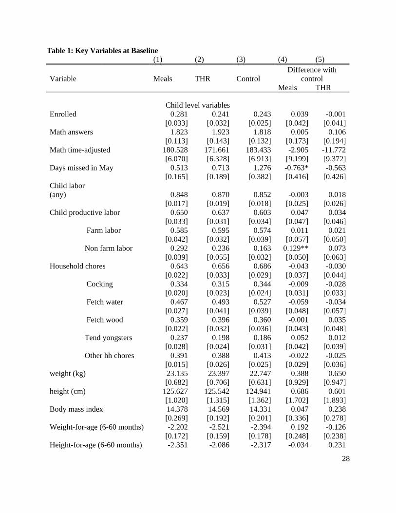
We summarize our key variables at baseline in table 1. The first three columns report the

9

averages for the villages with school meals, take home rations, and for the control villages. The last

two columns (4 and 5) report the tests whether these variables are statistically different across

treatment and control groups. We consider child level variables, which include educational, and

health outcomes as well as socioeconomic characteristics, and household level variables which

include the household head socioeconomic characteristics and household wealth.

It is apparent that prior to treatment, the groups were similar on most variables

including enrollment, child health and nutritional status, household and socioeconomic

characteristics. Out of the 86 differences reported in columns 4 and 5, there are 5 instances where

the estimated differences are statistically significant. Overall, we conclude that the random

assignment of villages to treatment and control groups was reasonably successful.

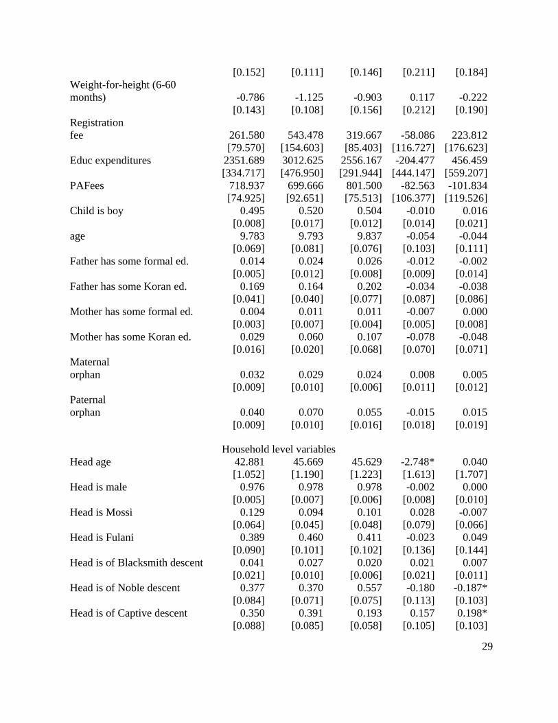
The anthropometric data are consistent with severe food shortage, with average weight-

for-age and height--for-age 2 standard deviations below the reference population4,5. The figures in

table 2 (top panel) indicate that prior to the treatment, more than half of children were

underweight or stunted, and about one third were wasted. Table 3 provides similar measures taken

from the 2003 Demographic and Health Survey (Institut National de la Statistique et de la

Démographie and ORC Macro, 2004) which is the most recent available national survey at the

time of our study. It can be seen that child malnutrition is widespread, and the northern region

(which includes our study area) is worse off than most other regions. Together, these figures

indicate that these households are facing severe constraints on nutrition and one could expect

significant gains from the program.

4. Empirical Model

Our primary interest is on reduced-form demand relations for child health outcome of

which anthropometric is one dimension. Such health demand function can be expressed as

dependent on food intake (itself a function of some exogenous variables such as prices), income,

endowments and child and household characteristics. Such demand function can be derived from

the constrained maximization of a unified household model in the tradition of Becker6 or from an

intra-household bargaining framework (e.g. Haddad, Hoddinott and Alderman, 1997). Thus

child health outcome is defined as a function of other child food intake (Ni), child characteristics

(Xi), household characteristics (Xh), and village level characteristics (Xv) such as health care

infrastructure and the availability of other public goods relevant to the child production function.

),,,( vhihihih XXXNHh = (1)

If we adopt a linear approximation for H, we can estimate the child health outcome as follows:

ivhtvthvtihvtihvtihvt XXXNh εβββββ +++++= 43210 (2)

We let child food intake depends on the household’s food intake (Fhvt) in period t and the

sharing rule δk (k=g, b) that governs the share of the household food intake which is allocated to

each child. For simplicity, we assume that the sharing rule varies only by gender.

hvtkkihvt FN δ=, , k=g, b (3)

Substituting back (3) in (2), child health outcome can be written as:

ivhtvthvtihvthvtkihvt XXXFh υβββλβ +++++= 4320 (4)

Where λk=β1δk

10

11

Together, equations 2, 3 and 4 offer a basis for understanding how the interventions

operate. For pre-school age children who are not participating into the programs directly, the

benefits of the program primarily come from increased F. However; the household can

neutralize the program effect on a child by choosing a sharing rule after the intervention so that

the child has the same food intake as before it. This is because the household food intake (F) in

regression (4) results from the utility maximization, and is a function of the exogenous variables

that govern food demand including income and prices. Since the interventions induce an

exogenous variation in F we are able to identify the parameter of interest. While we do not

observe prices our identification strategy relies on the random assignment of the villages to

treatment and control groups. Thus, any variation in prices will not be correlated with the

treatment variable and their omission will not bias the results. Note also, that the monthly

allocation in both programs is less than an individual – never mind a household – generally

consumes in a month. Thus the transfer is infra-marginal; both treatment and control groups are

expected to face the same marginal price.

Because the program was offered at the village level, we estimate the average intent to

treat (AIT) effect, that is, the impact of the program, on average, for all children in a given age

range within a village whether or not these children or their sibling took up the treatment.

This estimate measures the average program impact on eligible individuals (i.e. the impact of the

intervention instead of the impact of the treatment) and is relevant for two reasons. First, since in

practice policy makers have no influence on program participation, AIT is relevant for policy

analysis. Second, AIT provides a lower bound for average treatment on the treated (ATT) under

the assumption that the program impact on non participants in treatment groups is lower than its

effect on compliers.

Given that we have both a baseline and a follow up surveys, we could use a difference-in-

differences (DID) specification to estimate the program impact.

ivhtvihvtvkihvt RoundTXRoundTh υααβλβ +++++= 22* 2120 (5)

Where Tv is the treatment indicator, Xihvt is a vector of child characteristics (e.g, age), and

Round2 indicates the follow up survey. We estimate (5) controlling for village level fixed effects,

and for boys and girls. Because the eligibility for one program is for both boys and girls and for

the other it is for girls only, the appropriate control group differs for each program. Thus, the

regressions are not pooled.

During the follow up round, we used electronic scales instead of mechanical ones that were

used in the baseline. This improved measurement may introduce a spurious trend in our

anthropometric data. We argue, however, that in a regression using both rounds of the survey, the

trend will capture these types of variations due to improved scales during the follow up round.

Moreover, we also present results using only the follow up round. These results are not influenced

by the changes in the types of scales. Our empirical specification is then based on the following

regression:

ivhtvihvtvkihvt XTh υβλβ +++= 20 (6)

All variables are as defined previously. The impact of the program is given by λk. Our analysis then

compares age cohorts rather than changes in individuals over a panel. We present results using the

specification defined by equation 6 in the main text, but we include the DID estimation results using

both the baseline and the follow up data that corresponds to the main results of the study in the

appendix (Table A1)

12

13

Our identification strategy could be weakened if control communities are indirectly

affected by the program. For example, there could be cross over in which households in control

villages have their children attend school in treatment villages so that they gain access to the

program. Also households in the program villages could chose to foster in children from villages

without the programs. The former type of treatment contamination would lead, however, to an

underestimation of the program effects because some households in the control villages would

have access to the treatment. The latter impact is ambiguous; on the one hand the interventions

would induce an increase of household resources per child in control villages but if the foster

children enter our household sample their effect would depend on whether they were more or less

malnourished at baseline than were their counterparts. We will return to this issue when we

discuss our empirical results, but we note that, since the villages included in the impact evaluation

were only villages in which a new school was opened in the school year 2005-2006, control

villages are typically not neighboring villages of treatment villages, making cross-over less likely.

Moreover, as the survey indicates which child is fostered, we can check whether or results are

affected by the inclusion or exclusion of these children.

5. Results

5.1. Program impact7

As indicated in table 4, neither form of school based transfers led to a significant increase in the

weight for age of school age children. As mentioned above, these regressions are based on the

intention to treat – that is, the dummy variable for program availability indicates that the village

the child lived in received the intervention whether or not the child actually went to school.

Thus, there is no need to accommodate endogenous choice. Eligibility for THR further requires

14

that the household includes at least one girl of primary school age even if this girl is not in

school. Despite the absence of a larger weight increase for the sample as a whole, the girls age

10-15 have better nutritional status on average as measured by weight-for-age z-scores.

Table 5 addresses the spillover effect on younger siblings. In contrast to the results for

school age children the results for younger children show that both interventions lead to an

increase in weight for age of boys between 5 and 60 months of age, but did not have any

significant impact on girls of the same age group. While both of these increases are statistically

different from their respective control group, they are not statistically different from each other.

We exclude children under 6 months of age, who ideally should be reliant on breastfeeding,

preferably exclusive breastfeeding. The results are essentially the same when we restrict the

sample to children above 12 months and if we exclude children who are fostered. Moreover, the

results are similar for dry rations when we run the model as a difference in difference model

using village fixed effects. However, in the village fixed effects regression the school meal

impact on boys is no longer significant (see Table A1 in the appendix).8 The interventions did

not have any significant impact on height-for-age9.

As mentioned, for the regressions reported in table 5 young children are deemed eligible

for the take home rations if they live in a village randomly allocated to that intervention and if

they have a sister who is of school going age (6 -12). They are deemed eligible for school meals if

they live in a village randomly allocated to that intervention and if they have a brother or sister

who is of school going age. In both cases eligibility is not based on actual attendance, and thus is

not influenced by self selection.

Our analysis shows that the interventions had an impact on pre-school children (i.e. aged

6 to 60 months) who were not enrolled at the time of the survey, and who were not primarily

15

targeted by the interventions. From equation (3), we can conjecture that the spillovers observed

in table 5 could operate through two main channels. The first possible channel is an “income

effect” which is reflected by an increased food intake by the household (increased Fhvt). The

second channel is a “redistribution” effect, whereby the household modifies the food sharing

parameters (δ). For instance, if the household realizes that boys are worse off than girls in terms

of nutritional status, it could modify δ, to try to correct the initial imbalance10.

5.2. Robustness Check

We use regressions using children who were not eligible for the program yet in the

project sites to confirm that our results on the spillover to younger siblings are driven by the

interventions and not by third factors common to the community. One concern is that in a rural

area subject to frequent aggregate and individual income shocks, it is possible that a series of

shocks unrelated to the interventions generate the pattern that we observe. Moreover, other

interventions that target young children could have been in place, even if such interventions have

not been found during our field surveys. If either the shocks or the distribution of interventions

were not evenly distributed over the sample the results might be influenced by these factors. If

this were the case we would expect the estimated program impact to be similar when using

sample of children in the treatment sites that were ineligible since they are from households

where there is no school age child in a school meals village, or no school age girl in a dry rations

village. Barring substantial transfers across households, the interventions should not have

affected these children.

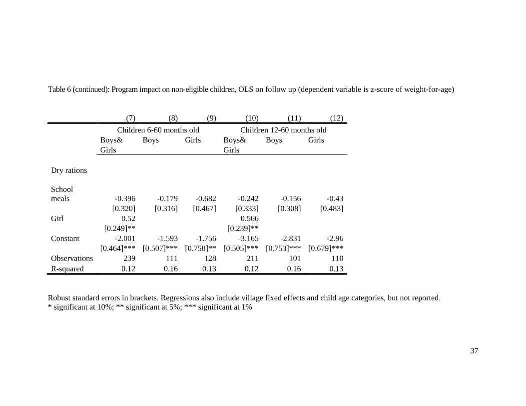
In table 6, we show the results of regressions similar to those in table 5. However, the

regressions in table 6 use a sample of non-eligible children. The results of the dry rations

villages are in columns 1-6, and the results of the school meals villages are in columns 7-12. For

all 12 regressions, the estimated program impact is not statistically different from zero,

suggesting that the interventions did not have any discernable effect on ineligible children. The

samples in table 6 are relatively small due to the filter employed. This contributes to a larger

variance of the coefficients than in the estimations reported in table 5. However, point estimates

in all the regressions reported are negative and this contrasts with those in table 5.

5.3. Comparing food and monetary transfers

Since our program impact estimate reflects both the income effect and the redistribution effect

we can estimate the monetary transfers that would have been required to produce the observed effect

in nutritional gains absent of redistribution to provide an approximation of the relative importance of

each of these effects. In particular, we calculate how much income transfer is needed to increase

child weight-for-age as much as the estimated program impact. We start by estimating to what extent

child nutritional status responds to household income. We follow the common approach in the

literature, and we presume that expenditures reflect a household’s long run income potential

(Haddad et al., 2003). Therefore we estimate nutritional status as a function of logged household

total expenditures as follows:

iiihih XEh εααα +++= 221 )ln( (7)

Where hi the outcome of interest, Ei is household total expenditures per adult and X is a

set of other variables including the education of the child’s mother and father. Since it is well

documented that expenditures is subject to substantial measurement errors, we address

measurement errors by instrumenting for total expenditures using the head count of household’s

16

17

livestock and fowls as instruments. Our rationale is that these variables are less subject to

measurement errors and are good predictors of total expenditures. However, because livestock

and fowls can be eaten, they may have a direct effect on nutritional status, thereby violating the

exclusion restriction. We verified, however, that most livestock and fowls are not directly

consumed, but rather sold11.

The IV estimation results are reported in table 7 (the first stage estimation is reported in

table A2 in the appendix). It can be inferred that girls’ weight-for-age (columns 3 and 6) is more

income elastic than boys’ weight-for-age (columns 2 and 5). These results are consistent with

other empirical studies in low income countries which found that investments in favored

demographic groups are less price and income elastic than investments in less favored

demographic groups. For example, Alderman and Gertler (1997) develop a theoretical model in

which investments in human capital are more income and price elastic for less favored children.

They showed empirically that the demand for medical care is more price and income elastic for

girls than for boys in Pakistan. Using household survey from India, Rose (1999) finds that

favorable rainfall shocks increase the probability that girls will survive more than they increase

the probability that boys will survive in rural India.

We use the response of weight-for-age reported in table 6 to estimate the increase in total

expenditures (in monetary terms) needed to achieve a gain in weight-for-age that is similar to the

program impact. The results are reported in CFA francs in table 8. The coefficient of the

logarithm of instrumented expenditures is within the range of those reported from household

surveys as well as similar estimates from country level regressions (Haddad et al. 2003). At

sample means and converting in US dollars, we find that $92 cash transfer per adult would be

18

needed to realize gains in weight-for-age similar to the dry ration impact on boys and girls

(.341), and $57 would be needed to realize a gain similar to the impact of school meals (.195).

The food transfers expressed in monetary value were, however, much smaller: $4.70 and $7.15

per adult under the dry ration intervention and the school meals intervention, respectively (see

table 8 for details).

Taken together, these results convey two main sets of information. First, in-kind

transfers have a larger impact on child nutritional status than that would have been achieved

under an equal size cash transfers. This would be consistent with the theoretical argument by

Ross (1991) who shows that in-kind transfers (in the absence of a resale market) may be more

effective than cash transfers at raising the welfare of all household members when parents put

insufficient weight on children welfare than society would have preferred12. Second, the program

impacted boys predominantly, while the analysis of weight-for-age response to total expenditures

showed that boys’ nutritional status is not any more responsive to income than is girls’

nutritional status. Thus, one can argue that if the interventions consisted of cash transfers and

further that marginal allocation from cash transfers do not differ from the results in cross

sectional regressions of total income the impact would have been as large or larger for girls.

There is however, one caveat to this interpretation. Households could change the sharing rule (δ)

in way that allocates relatively more of the additional food to boys. This could be the case if

biological factors explain in part why girls fare better than boys in terms of nutrition (e.g.

Wamani et al, 2007) and households are concerned about equity.

5.4. Cost-effectiveness

In table 9, we compare the program impacts to its costs. This cost-effectiveness analysis

19

assesses how large the program effects are on a per-dollar basis. The cost estimates have been

provided by WFP and include the food costs and the operation costs, and are expressed in US

dollar13. The results are expressed in terms of additional gain in standard deviations of weigh-

for-age per one US dollar. Focusing on boys (on whom the estimated impact is significant), the

return from dry rations (.026) is twice as large as the return from school meals (.012). And these

results are similar when we look only at children aged 12 to 60 months.

From this analysis, it appears that dry rations are more cost-effective than school meals if

the objective is to improve the nutritional status of pre-school age children. School feeding

interventions, however, may have other objectives (e.g. increase enrollment and retention) so that

comparing take home rations and school meals requires looking at other outcomes as well.

6. Discussion

The increase in the weight of younger siblings of the children eligible for either school

based transfer is relatively large. Indeed, it exceeds that which might be predicted on the basis of

an income transfer alone. Using the parameters on instrumented expenditure in table 7 it would

take a transfer equivalent to 98 percent of income per adult to achieve the same impact that dry

rations have on boys aged 6 to 60 months (0.57 increase in the z-score). Reaching the impact of

school meal on the same group of children (0.42 increase in z-score of weight-for-age) would

require an increase in household expenditures by 69 percent. In comparison, over the 9 month

period of the academic year, the THR per adult is equivalent to a 2 percent of average household

expenditures per adult, and the school meal is equivalent to 5 percent of average household

expenditures per adult. The estimated effect of household expenditures on weight-for-age in our

sample is larger than the median observed in a dozen similar estimates from household data

20

(Haddad, et al. 2003).

A relevant question is why the food transfer impact is much larger than the estimated

impact from a same size cash transfer. It is plausible that food for education programs achieve

an improvement on nutrition beyond the average impact of expenditures through a labeling effect

by which a program encourages a reallocation of household resources (Kooreman, 2000). Such

an increase of allocation towards food and nutrition beyond the pre-program marginal budgets

has been observed for food stamps in the United States (Breunig and Dasgupta, 2005; Fraker,

Martini, and Ohls, 1995) and for cash transfers in Ecuador (Paxson and Schady, 2008)14. The

data do not allow us to distinguish the impact of the mode of transfer (in kind as opposed to

cash) from the linkage to schools and, thus, to children. However, the fact that this impact on

nutrition of young children is relatively large is clearly indicated.

While a 100% ‘flypaper effect’ (as Jacoby (2002) deems it) would imply no increase in

overall consumption by the rest of the household it does not rule out a reallocation of this

consumption. However, the fact that none of the school feeding programs had an impact on the

nutritional status of school age children (table 4) seems to support the impact occurring within

the household allocation of resources and not at the school itself.15

Nor would a concentration of additional resource on younger children be an undesirable

outcome. Despite the concern with leakage of school meals in the literature it is questionable

whether increasing the weight of school aged children who have previously been malnourished is

desirable (Victoria et al., 2008); there is no doubt regarding such an objective for younger

children.

7. Conclusion

21

In this paper, we have used a prospective randomized design to assess the impact of two

school feeding schemes on health outcomes of pre-school age children from low income

households in northern rural Burkina Faso. We considered two programs: school meals which

provide lunch in school, and take home rations which provide girls with 10 kg of cereal flour each

month, conditional on 90 percent attendance rate. While the interventions were design to directly

target school age children (who are enrolled), we focus on children who were too young to be

enrolled at the time of the survey. Therefore, our study provides direct measures of spillovers effects

within the household. Moreover, because we have a randomized experiment, we can interpret the

estimated impact as causal.

After the program ran for one academic year, we found that take-home rations have

increased weight-for-age by 0.34 standard deviations for boys and girls under age 5 taken jointly

and by 0.57 standard deviations for boys taken separately. The school meals intervention has

increased weight-for-age by 0.40 for boys. Neither program had a significant impact on girls

taken separately.

When we contrast those findings with the health outcome response to household total

expenditures, we make two observations. First, consistent with previous studies, we show in our

data that on average girls’ health outcome is more responsive to household income than is boys’

health outcome. The interventions, however, affected boys only. Second, to realize similar gains

in health outcomes through increased household income would have required cash transfer about

9 times the value of the take home rations. It is apparent that in-kind transfers have a larger

effect on child health outcome than general sources of income and are allocated differently than

the household’s other resources.

22

Our results show that the spillovers effects of school feeding interventions on young

children are relatively large, as compared to the direct effects. This could be because in the short-

run, the weight-for-age is more elastic for younger children than for school age children. While

both interventions generated positive impacts on boys, we found that dry rations are most cost-

effective than school meals: a dollar in dry rations and school meals earns a gain in weight-for-

age of 0.026 and 0.012 standard deviations, respectively. While school feeding programs may not

be the first best choice to address malnutrition for pre-school age children in a food insecure

region, they do have a measurable impact. Failing to account these effects likely under-estimate

the total benefits of school feeding programs, which include schooling and the indirect income

support to target populations as well as the contribution to nutrition of younger children.

23

References

Adelman, Sarah, Daniel O. Gilligan and Kim Lehrer. 2008. How Effective are Food for

Education Programs? A Critical Assessment of the Evidence from Developing Countries.

Forthcoming. IFPRI Food Policy Review No. 9 (Washington, DC: International Food

Policy Research Institute).

Afridi, Farzana. 2009. Child Welfare Programs and Child Nutrition: Evidence from a Mandated

School Meal Program in India. Forthcoming, Journal of Development Economics

Ahmed, Akhter U. 2004. Impact of Feeding Children in School: Evidence from Bangladesh.

Washington, DC: International Food Policy Research Institute. Processed.

Akresh, Richard. 2009. Flexibility of Household Structure: Child Fostering Decisions in Burkina

Faso. Journal of Human Resources. 44: 976-997

Alderman, H., P. A. Chiappori, L. Haddad, J. Hoddinott, R. Kanbur. 1995. Unitary Versus

Collective Models of the Household: Time to Shift the Burden of Proof? World Bank

Research Observer 10(1): 1-20.

Alderman, H. and P. Gertler. 1997. "Family Resources and Gender Differences in Human

Capital Investments: The Demand for children's Medical Care in Pakistan". In Haddad,

Hoddinott, and Alderman (eds.) Developing Countries: Models, Methods and Policies.”

Johns Hopkins University Press, Baltimore.

Beaton, G. and H. Ghassemi: 1982. Supplementary Feeding Programs for Young Children in

Developing Countries. American Journal of Clinical Nutrition. 34: 864-916.

Breunig, Robert and Indraneel Dasgupta. 2005. Do Intra-household Effects Generate the Food

Stamp Cash-Out Puzzle? American Journal of Agricultural Economics. 87(3): 552-68.

24

Currie, Janet and Firouz Gahvari. 2008. Transfers in Cash and In-Kind: Theory Meets the Data.

Journal of Economic Literature. 46(2): 333-383.

Fraker, Thomas (1990). “Effects of Food Stamps on Food Consumption: A Review of the

Literature.” Washington, DC: Mathematica Policy Research, Inc.

Fraker, Thomas, Alberto Martini and James Ohls. 1995. The Effect of Food Stamp Cashout on

Food Expenditures: An Assessment of the Findings from Four Demonstrations. Journal

of Human Resources. 30(4): 633-49.

Haddad L., H. Alderman, S. Appleton, L. Song and Y. Yohannes. 2003. “Reducing Child

Malnutrition: How Far Does Income Growth Take Us?” World Bank Economic Review

17(1): 107-131.

Haddad, J., J. Hoddinott and H. Alderman. 1997. “Intra-household Resource Allocation in

Developing Countries: Models, Methods and Policies.” Johns Hopkins University Press,

Baltimore.

Hoynes, Hilary W. and Diane Schanzenbach. 2009. Consumption Reponses to In-Kind

Transfers: Evidence from the Introduction of the Food Stamp Program. American

Economic Journal: Applied Economics. Forthcoming

Jacoby, Hanan G. 2002. Is there an intrahousehold “flypaper effect”? Evidence from a school

feeding programme. Economic Journal 112 (476):196–221.

Kazianga, Harounan, Damien de Walque and Harold Alderman. 2009. Educational and Health

Impact of Two School Feeding Schemes: Evidence from a Randomized Trial in rural Burkina

Faso. World Bank. Policy Research Working Paper Series # 4976.

Kooreman, Peter. 2000. The Labeling Effect of a Child Benefit System. American Economic

Review 90(3): 571-583.

25

Kristjansson EA, Robinson V, Petticrew M, MacDonald B, Krasevec J, Janzen L, Greenhalgh T,

Wells G, MacGowan J, Farmer A, Shea BJ, Mayhew A, Tugwell P. School feeding for

improving the physical and psychosocial health of disadvantaged elementary school

children. Cochrane Database of Systematic Reviews 2007, Issue 1. Art. No.: CD004676.

See http://www.cochrane.org/reviews/en/ab004676.html.

Paxson, Christina and Norbert Schady. 2008. Does Money Matter? The Effects of Cash

Transfers on Child Health and Cognitive Development in Rural Ecuador. Processed.

Ross, T., 1991 “On the Relative Efficiency of Cash Transfers and Subsidies,” Economic Inquiry.

29(3): 485-496.

Rosenweig, Mark R. 1986. Program Interventions, Intrahousehold Distribution and the Welfare

of Individuals: Modeling Household Behavior. World Development. 14(2): 233-243

Shrimpton R, Victora C, de Onis M, Costa Lima R, Blössner M, Clugston G. 2001. Worldwide

Timing of Growth Faltering: Implications for Nutritional Interventions. Pediatrics. 107;

75-81.

Svedberg, P. 1990. Undernutrition in Sub-Saharan Africa: Is there a gender bias? Journal of

Development Studies 26 (3): 469-486.

Victora CG, Adair L, Fall C, Hallal PC, Martorell R, Richter L, Sachdev HS. 2008. Maternal

and Child Undernutrition Study Group. Maternal and child undernutrition: consequences

for adult health and human capital. Lancet. 371(9609):302

Wamani, H., A. N. Astrom. S. Peterson J. K. Tumwine and T. Tylleskar. 2005. Boys are More

Stunted than Girls in Sub-Saharan Africa: A Meta Analysis of 16 Health and

Demographic Surveys. BMC Pediatrics. 7:17

26

WHO Multicentre Growth Reference Study Group. WHO Child Growth Standards. 2009.

Length/height-for-age, weight-for-age, weight-for-length, weight-for-height and body

mass index-for-age: Methods and development. Geneva: World Health Organization,

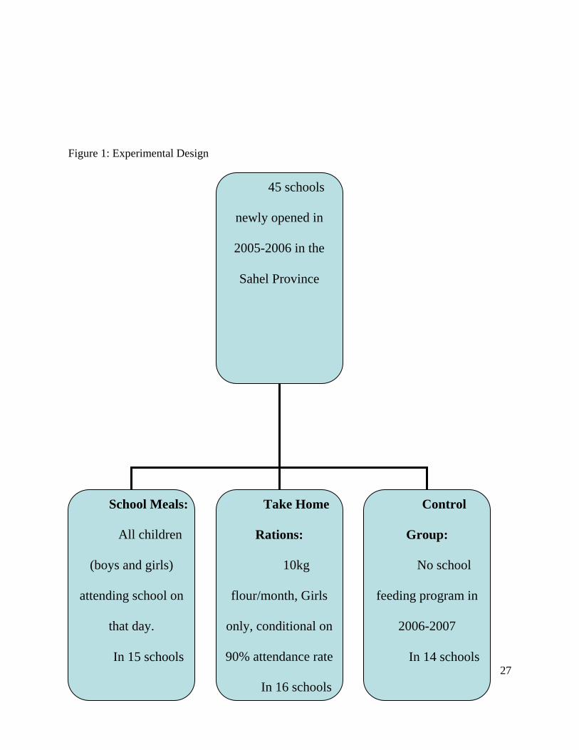
Figure 1: Experimental Design

45 schools

newly opened in

2005-2006 in the

Sahel Province

27

School Meals:

All children

(boys and girls)

attending school on

that day.

In 15 schools

Take Home

Rations:

10kg

flour/month, Girls

only, conditional on

90% attendance rate

In 16 schools

Control

Group:

No school

feeding program in

2006-2007

In 14 schools

28

Table 1: Key Variables at Baseline (1) (2) (3) (4) (5)

Variable Meals THR Control Difference with

control Meals THR

Child level variables Enrolled 0.281 0.241 0.243 0.039 -0.001

[0.033] [0.032] [0.025] [0.042] [0.041] Math answers 1.823 1.923 1.818 0.005 0.106

[0.113] [0.143] [0.132] [0.173] [0.194] Math time-adjusted 180.528 171.661 183.433 -2.905 -11.772

[6.070] [6.328] [6.913] [9.199] [9.372] Days missed in May 0.513 0.713 1.276 -0.763* -0.563

[0.165] [0.189] [0.382] [0.416] [0.426] Child labor (any) 0.848 0.870 0.852 -0.003 0.018

[0.017] [0.019] [0.018] [0.025] [0.026] Child productive labor 0.650 0.637 0.603 0.047 0.034

[0.033] [0.031] [0.034] [0.047] [0.046] Farm labor 0.585 0.595 0.574 0.011 0.021

[0.042] [0.032] [0.039] [0.057] [0.050] Non farm labor 0.292 0.236 0.163 0.129** 0.073

[0.039] [0.055] [0.032] [0.050] [0.063] Household chores 0.643 0.656 0.686 -0.043 -0.030

[0.022] [0.033] [0.029] [0.037] [0.044] Cocking 0.334 0.315 0.344 -0.009 -0.028

[0.020] [0.023] [0.024] [0.031] [0.033] Fetch water 0.467 0.493 0.527 -0.059 -0.034

[0.027] [0.041] [0.039] [0.048] [0.057] Fetch wood 0.359 0.396 0.360 -0.001 0.035

[0.022] [0.032] [0.036] [0.043] [0.048] Tend yongsters 0.237 0.198 0.186 0.052 0.012

[0.028] [0.024] [0.031] [0.042] [0.039] Other hh chores 0.391 0.388 0.413 -0.022 -0.025

[0.015] [0.026] [0.025] [0.029] [0.036] weight (kg) 23.135 23.397 22.747 0.388 0.650

[0.682] [0.706] [0.631] [0.929] [0.947] height (cm) 125.627 125.542 124.941 0.686 0.601

[1.020] [1.315] [1.362] [1.702] [1.893] Body mass index 14.378 14.569 14.331 0.047 0.238

[0.269] [0.192] [0.201] [0.336] [0.278] Weight-for-age (6-60 months) -2.202 -2.521 -2.394 0.192 -0.126

[0.172] [0.159] [0.178] [0.248] [0.238] Height-for-age (6-60 months) -2.351 -2.086 -2.317 -0.034 0.231

29

[0.152] [0.111] [0.146] [0.211] [0.184] Weight-for-height (6-60 months) -0.786 -1.125 -0.903 0.117 -0.222

[0.143] [0.108] [0.156] [0.212] [0.190] Registration fee 261.580 543.478 319.667 -58.086 223.812

[79.570] [154.603] [85.403] [116.727] [176.623] 51.689 12.625 56.167 4.477 6.459

[334.717] [476.950] [291.944] [44 7] 937 .666 00 -82.563 3425] .651] 3] 26]

hild is boy 0.495 0.520 0.504 10 016[0.012] [0.014] [0.021]

-0.054

e formal ed.

an ed.

al ed.

ome Koran ed. [0 [0 [0 [0.071]

al

Household level variables

nt

ptive descent

Educ expenditures 23 30 25 -20 454.147] [559.20

-101.87]

PAFees 718.[74.9

699[92

801.5[75.51 [106.37

-0.0[119.5

0.C[0.008] [0.017]

age 9.783 9.793 9.837 -0.044[0.069] [0.081] [0.076] [0.103]

-[0.111] -Father has som 0.014 0.024 0.026 0.012 0.002

[0.005] [0.012] [0.008] [0.009] [0.014] Father has some Kor 0.169 0.164 0.202 -0.034 -0.038

[0.041] [0.040] [0.077] [0.087] [0.086] Mother has some form 0.004 0.011 0.011 -0.007 0.000

[0.003] 0.029

[0.007] 0.060

[0.004] 0.107

[0.005] -0.078

[0.008] -0.048Mother has s

Matern.016] .020] .068] [0.070]

orphan 0.032 0.029 0.024 0.008 0.005[0.009] [0.010] [0.006] [0.011] [0.012]

Paternal orphan 0.040

[00.070

[00.055

[0-0.015 0.015

[0.019] .009] .010] .016] [0.018]

Head age 42.881[1

45.669[1

45.629[1

-2.748* [

0.040[ .052] .190] .223] 1.613] 1.707]

Head is male 0.976[0

0.978[0

0.978[0

-0.002 [

0.000[ .005] .007] .006] 0.008] 0.010]

Head is Mossi 0.129[0

0.094[0

0.101[0

0.028 [

-0.007[0 .064] .045] .048] 0.079] .066]

Head is Fulani 0.389[0

0.460[0

0.411[0

-0.023 [0

0.049[0 .090] .101] .102] .136] .144]

Head is of Blacksmith desce 0.041[0

0.027[0

0.020[0

0.021 [

0.007[ .021] .010] .006] 0.021] 0.011]

Head is of Noble descent 0.377[

0.370[

0.557[

-0.180 [0

-0.187*[0 0.084] 0.071] 0.075] .113] .103]

Head is of Ca 0.350

0.391

0.193

0.157 [0

0.198*[0 [0.088] [0.085] [0.058] .105] .103]

30

Head is -0.020 -

CF) [12.659] [19.772] [6.027] [14.020] [20.670]

Muslim 0.967 0.978 0.98 0.009[0.018] [0.012] [0.007] [0.019] [0.014]

Household asset value (1000 66.522 92.109 78.966 -12.443 13.143

R ets. * significant *** s nt at 1 USD = +/- 500 CFA Francs. M lani are two ethnic groups from the region. B smith, Noble or Captive desc aste cat ou i

ethnic groups.

obust standard errors in brack Significant at 10%; ** at 5%, ignifica 1%

ossi and Fulack ent are c s used to egorize h seholds w thin these

T dren t andard ation the (z-scores: children between 6 and 60 months ol

) (2) (W -age t-for H -A

ine (u eight) ted) ) School meals .6 29.Take Home Rations 32.3 60.0 Control 55.3 31.6 6

o standard deviation below the median in rural Burkina

Ouagadougou (area) 17.9 12.4 16.4 486 North 41.8 19.4 41.7 1587 East 38.4 18.7 47.2 2147 West 37.6 19.3 35.7 2328 Central/South 38.4 19.2 35.1 1722 Total Rural 40.3 19.7 41.4 7166

Source: ORC Macro, 2008. MEASURE DHS. STATcompiler.

http://www.measuredhs.com, August 1 2008.

able 2: Percentage of chil wo st devi below mediand)

(1 3) eight-for Weigh -Height eight-for ge

Basel nderw (was (stunted

52 5 59.9 56.2

1.7

Table 3: Percentage of children twFaso, 2003 (z-scores: children between 0 and 60 months old)

Weight-for-age

Weight-for-height Height-for-age N

Region (underweight) (wasted) (stunted)

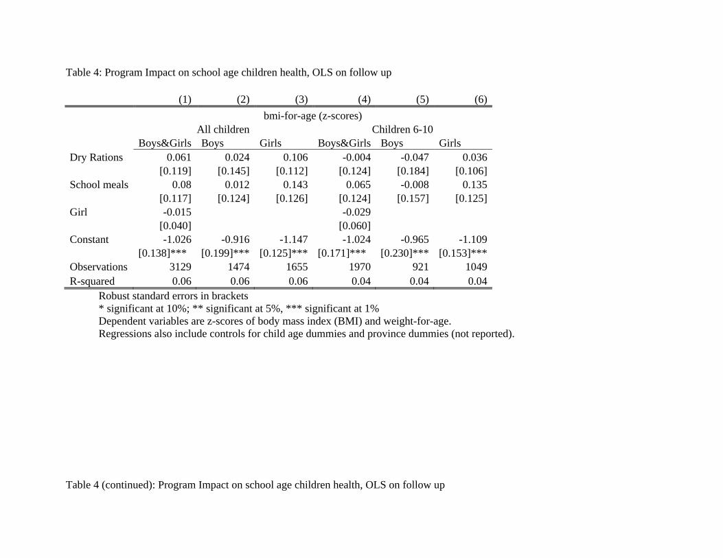
Table 4: Program Impact on school age children health, OLS on follow up

(1) (2) (3) (bmi-for-age (z )

(4) (5) 6)-scores

All children Childre 0 Boys&Girls Boys Girl Boys&Girls Boys Girls

Dry Rations 0.061 0.024 06 -0.004 -0.047 0.0

n 6-1s

0.1 36[0.119] [0.145] 8 [0.10

School meals 0.08 0.012 0 0.1[0.117] [0.124] [0.124] [0.15 .12

Girl -0.015 -0.029[0.040] [0.060]

Constant -1.026 -0.916 -1.024 -0.96 -1.1[0.138]*** [0.199]*** [0.1 [ [0.153]*

Observations 3129 1474 921 10R-squared 0.06 0.06 0.04 0. 0.

[0.112]0.143

[0.126]

-1.14725]***

16550.06

[0.10.

24]065

[0.1-0.

4] 08 7]

5

6]355]

09**4904

[0

0.171]*** [0.230]*** 1970

04 Robust standard errors in brackets * significant at 10%; ** significant at 5%, *** significant at 1% Dependent variables are z-scores of bod ndex (BMI) and weight-for-ageRegressions also include controls for chi dummies and province dummi

Table 4 (continued): Program Impact on school age children health, OLS on follow up

y mass ild age

. es (not reported).

33

weight-for-age (z-scores) (7) (8) (9)

Children 1 5 Boys&Girls Boys

Dry Rations 0.204 0.247

0-1Girls

0.116[0.197] [0.208] 217]

0[0.

tant -2.464 -2.328[0.158]***

ons R-squared

[0.School meals 0.122 0.071 0.159

[0.200] [0.197] [0.223]Girl .182

063]*** Cons -2.496

[0.142]*** [0.175]***Observati 2053 966 1087

0.08 0.08 0.07Robust standard in bra

nificant at 1 * signi at 5%, *** significant at 1% body m ss index (BMI) and weight-for-age.

ince dummies (not reported).

errors ckets * sig 0%; * ficantDependent variables are z-scores of aRegressions also include controls for child age dummies and prov

Table 5: Program Im ol age children nutritional status, OLS on follow up (dependent variable is z-score of weight-for-

age)

(4) (5) (6)ren 6- ths Children 12-60 months

pact on prescho

(1) (2) (3)Child 60 mon

Boys Boys&Girls Boys GirlsDry Rations 0.570 0.070 0.321 0.567 0.044

[0.191]*** [0.193] [0.157]* [0.184]*** [0.191]als

Girl 0.177 0.147[0.107] [0.109]

Consta -1.609 -2.52 -2.972 -1.929297]*** [0.252]***

Observ 318R-squa

&Girls Boys Girls0.341

[0.163]** School me

nt -2.264 -2.576[0.286]*** [0.391]*** [0.408]*** [0.215]*** [0.

ations 720 385 335 678 360 red 0.06 0.09 0.07 0.06 0.1 0.06

Robust standard errors in brackets. Regressions also include village fixed effects and child age categories, but not reported. * significant at 10%; ** significant at 5%; *** significant at 1%

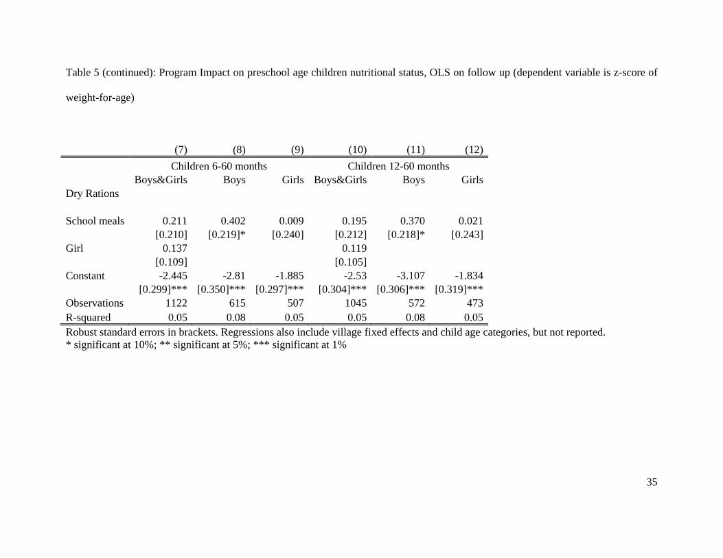
35

ht-for-age)

( ( (

Table 5 (continued): Program Impact on preschool age children nutritional status, OLS on follow up (dependent variable is z-score of

weig

(7) (8) (9) 10) 11) 12)Children 6-60 months Children 12-60 months

Boys&Girls Boys Girls Boys&Girls Boys GirlsDry Rations

School meals 0.211 0.402 0.009 0.195 0.370 0.021[0.210] [0.219]* [0.240] [0.212] [0.218]* [0.243]

Girl 0.137 0.119[0.109] [0.105]

Constant -2.445 -2.81 -1.885 -2.53 -3.107 -1.834[0.299]***

1[0.350]*** [0.297]*** [0.304]***

1[0.306]*** [0.319]***

Observations 122 615 507 045 572 0

473R-squared 0.05 0.08 0.05 0.05 .08 0.05Robust standard errors in brackets. Regressions also include village fixed effects and child age categories, but not reported. * significant at 10%; ** significant at 5%; *** significant at 1%

36

(1) (2) (3) (4) (5) (6)Children 6-60 months old Children 12-60 months old

Table 6: Program impact on non-eligible children, OLS on follow up (dependent variable is z-score of weight-for-age)

Boys& Boys Girls Boys& Boys irls Girls Girls

G

Dry rations -0.095 -0.074 -0.108 -0.088 -0.112 -0.058[0.223] [0.293] [0.270] [0.236] [0.320] [0.279]

[0. [0.2

[0. 0. . 4 2 2

School meals

Girl 0.418 1

0.370097]** 4]*

Constant -1.798 [0.327

-2.074[0.417]

-1.207[0.517]

-2.156335]*

-2.060520]**

-1.902455]**]*** *** ** ** [ * [0 *

Observations 487 241 246 35 20 15R-squared 0.04 0.03 0.04 0.04 0.04 0.03

Robust standard errors in brackets. Regressions also include village fixed effects and child age categories, but not reported. * significant at 10%; ** significant at 5%; *** significant at 1%

37

Table 6 (continued): Prog impact on n-eligible ildren, OL n follow u dependent riable is z-score of weight-for-age)

(7) (8) (9) (10) (11) (12)

ram no ch S o p ( va

Children 6-60 months old Children 12-60 months old Boys& Boys Girls Boys& Boys Girls Girl Girl s s

Dry rations

ol -0.179 -0.682 -0.156 -0.43

[0.316] [0.467] [0.308] [0.483]

-2 -1 -1 -3 -2 -[0.464]*** [0.507]*** [0.758]** [0.505]*** [0.753]*** [0.679]***

Observations 239 111 128 211 101 110

Schomeals -0.396 -0.242

[0.320] [0.333]Girl 0.52 0.566

[0.249]** [0.239]**Constant .001 .593 .756 .165 .831 2.96

R-squared 0.12 0.16 0.13 0.12 0.16 0.13

Robust standard errors in brackets. Regressions also include village fixed effects and child age categories, but not reported. * significant at 10%; ** significant at 5%; *** significant at 1%

Table 7: Child health response to household expenditures (dependent variable is z-score of weight-for-age)

(1) (2) (3) (4) (6)6 to 60 months 12 to 60

(5)months

Boys&Girls Boys Girls Boys&Girls Boy Girls s

lnExpCap 0.720 0.581 0.937 0.733 0.345 1.125[0.284]** [0.384] [0.431]** [0.285]** [0.353] [0.460]**

Girl 0.113 0.089[0.079] [0.083]

Constant -9.984 -8.651 -11.759 -10.496 -6.463 -14.175[3.953] [5.026]***

Observations 1579 828 692[3.161]*** [4.358]** [4.661]** [3.144]***

751 1457 765

Standard rs in bra ressions also child age, m er and fath ducation levels, household characteristics, and village fixed effects. * significant at 10%; ** significant at 5%; * fican

erro ckets. Reg oth er e

** signi t at 1%

39

(1) (2) (3) (4) (5) (6) Children 6-60 months Children 12-60 months

Table 8: Increase in expenditures required for the same impact as the interventions

Boys&Girls

ys irls Boys&Gis

Boys Girls

(1)School meals

09 0.370 0.021

Bo G rl

0.211 0.402 0.0 0.195

[0.210] 0.21 [0 [0 8]* ](rations

0 6 4

[0.163 191]*** [0.193] [0 [0.184]*** [0.191]

Per adult expenditures e t proimpact

(3) School 28486 67257 934 25859 104249 1814

rations69 159754 3802

Per household expenditure increase required to achieve program impact (5) School meals

133886 316109 4388 121539 489970 8528

(6) Dry rations

216376 448214 34131 200073 750845 17868

[ 9]* .240] .212] [0.21 [0.2432) Dry 0.341 .570 0.070 0.321 0.5 7 0.04

]** [0. .157]*

increas required o achieve gram

meals

(4) Dry 46037 95365 7262 425

In rows 3 and 4, the figure in each cell is the ratio of the estimated program impact to the

corresponding marginal value of the regression of weight-for-age on expenditures (taken at the

sample mean).

In rows 5 and 6, the corresponding figure is multiplied by the number of adults in the household.

40

ool meals Dry R

Table 9: Cost-effectiveness analysis

Schations

Annual transfe p (U 41.46r er student SD)* 51.37Number of students per household 0.81 n.r.

emale students per

Annual program cost size per

cost per adult (USD)

7.15 4.70

Program Impact (Children 6-60

Boys 0.402 0.570.

Boys and Girls 0.0063 0.0150.0.0003 0.003

Program Impact (Children 12-60

00.370 0.567

Girls 0.021 0.044eight-for $ 1**

0.0058 0.015 Boys 0.0110 0.026

Number of fhousehold

n.r. 0.43

household Annual program

33.58 22.09

months) Boys and Girls 0.211 0.34

Girls Gains in weight-for-age per $ 1**

009 0.07

Boys Girls

0120 0.026

months) Boys and Girls Boys

.195 0.321

Gains in w Boys and Girls

-age per

Girls 0.0006 0.002* Figures include food costs and operation costs. Figures are provided by WFP office in Ouagadougou ** Gains in standard deviatn.r. = not relevan

ions of weight-for-age t.

Appendix

Table A1: Program Impac z-scor

weight-for-age)

(1) 2 ( (4) (5 (6)Children 6-60 m onths old

t on pr

(

e-sch

)onths old

ool age child

3)

ren nutritional

Children 12-60 m

status, OLS

)

on two rounds (dependent variable is e of

Boys& Boys irls Boys& oys Girls Girls Girls

Dry Rations 0.461 6 0.419 0.491 0.508 0.447

0.4

G

3

B

[0.181]** [0.24 0.270] [0.182]*** [0.242]** [0.273] School Meals

Round2 1.097 1.092 1.035[0.127]*** [0.164]*** * [0.164]*** [0.197]***

Girl 0.162 [0.086]* [0.087]*

Constant -2.907 -3.081 -2.448 -3.425 -3.432 -3.294[0.248]*** [0.336]*** * [0.288]*** [0.250]***

Observations 1356 719R-squared 0.21 0.27 0.21 0.21 0.27 0.20

3]*

1.174

[

[

[

1.96]

049***

1.1740.1 [0.127]**

0.156

0.388]***637

[0.197]**1305 688 617

Robust standard errors in brackets. Regressions also include village fixed effects and child age categories, but not reported. * significant at 10%; ** significant at 5%; *** significant at 1%

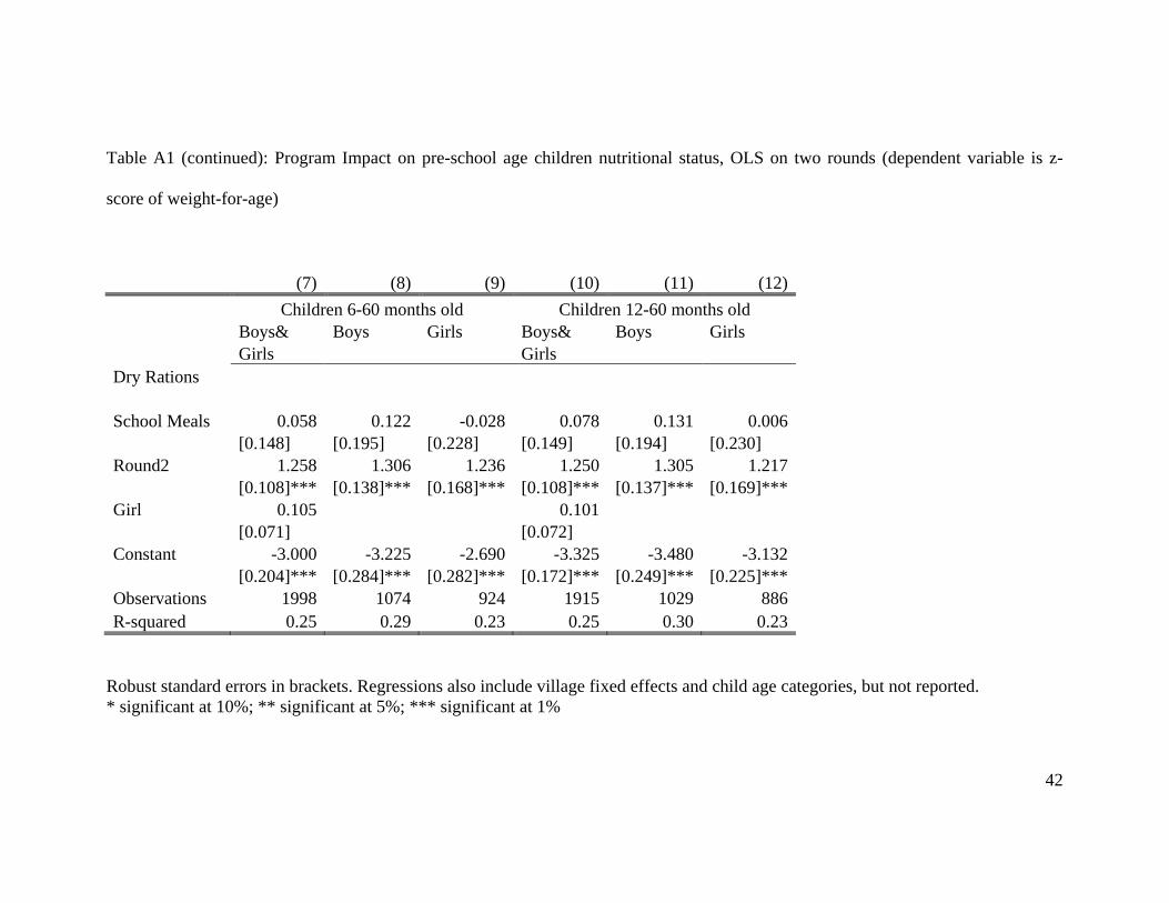
42

Table

or-age)

( ( (

A1 (continued): Program Impact on pre-school age children nutritional status, OLS on two rounds (dependent variable is z-

score of weight-f

(7) (8) (9) 10) 11) 12)Children 6-60 months old Children 12-60 months old

Boys& Boys Girls Boys& Boys Girls Girls Girls

Dry Rations

School Meals 0.058 0.122 -0.028 0.078 0.131 0.006[0.148] [0.195] [0.228] [0.149] [0.194] [0.230]

Round2 1.258 1.306 1.236 1.250 1.305 1.217[0.108]*** [0.138]*** [0.168]*** [0.108]*** [0.137]*** [0.169]***

Girl 0.105 0.101[0.071] [0.072]

Constant -3.000 -3.225 -2.690 -3.325 -3.480 -3.132[0.204]*** [0.284]***

1[0.282]*** [0.172]*** [0.249]***

1[0.225]***

Observations 1998 074 924 1915 029 886R-squared 0.25 0.29 0.23 0.25 0.30 0.23

Robust standard errors in brackets. Regressions also include village fixed effects and child age categories, but not reported. * significant at 10%; ** significant at 5%; *** significant at 1%

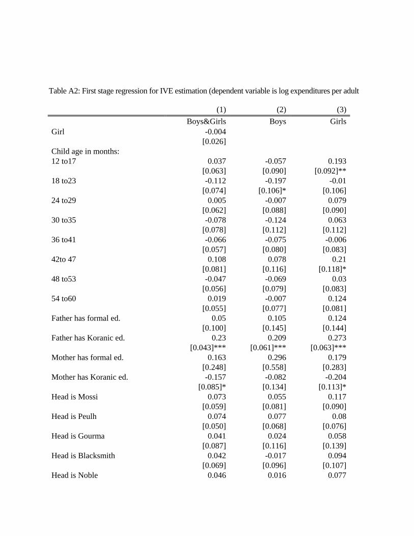
Table A2: First stage regression for IVE estimation (dependent variable is log expenditures per adult

(1) (2) (3) Boys&Girls Boys Girls

Girl -0.004 [0.026]

Child age in months: 12 to 0.037 -0.057 0.193

[0.063] [0.090] .092]**18 to - -0.01

06 [0.106]24 to .0 .007 0.079

06 088] [0.090]30 to - 0.063

[0.112]36 to .0 .075 -0.006

05 080] [0.083]42to 0.108 0.078 0.21

[048 to 9 0.03

05 079] 083]54 to

[0 081]Father has formal ed.

10 145] 144]Father has Koranic ed. 0 .209

4 ]***Mother has formal ed.

558] 283]Mother has Koranic ed. .1 .082 .204

[0.085]* [0.134] 13]*Head is Mossi

090]Head is Peulh .0 .077 0.08

05 068] 076]Head is Gourma 0.041 0.024

[0.087] [0.116] 139]Head is Blacksmith 2 -

[0.069] [0 107]Head is Noble 6

17

23

29

35

41

47

53

60

[0

[0.118]*

[0.

0.1.07

124]052]

-[0.1

-0[0.

0.197]*[0

0[0.

0.0.07

788]667]

-[0-0

[0.

0.12.11

42][0

-0[0.

.080.0

1]476]

[0-0

[0.-0.007

.11.06

6]-

[0.0.019

[0.0.124

[0.0.124

[0.0.273

0630.179

[0.-0

[0.10.117

[0.

[0.0.058

[0.0.094

[0.0.077

.050.

5]050]

.23

[00

[0.0

.07.1

7]05

[0.

[0.0 3]*0.124

**638]57

[0.061

[0.-0

]**0.29

*6

[0.-0

0.0.05

739]740]

0.05.081

5][0

0[0.

[00

[0.

0.04

0.04

0.01.090.01

76]6

44

[0.052] [0.070] [0.080]Head is Captive 0.047 0.097 -0.002

[0.061] [0.085] [0.092]Head is Muslim 0.167 -0.037 0.43

Instruments Cattle 0.0 0.0 0.0

[0.01 [0.011 0.038 0.025

[0.0 [0.009]*** [0.009]***0.011 0.012 0.008

[0.00 [0.0 [0.Guinea fowls

[0.0 [ [0.01Chicken

[0.00 [0.0 [0.00Constant

[0.1 [0.1 [0.17Observations

d standard errors in brackets. Regressions also illage fixe s but not re

ant at 10%; ** significant at 5%; *** significant at 1%

[0.088]* [0.120] [0.134]***

38 38 39 [0.008]*** 1]*** ]***

Sheep 0.03 06]***

Goat 3]*** 04]*** 004]*0.026 0.015 0.042

09]*** 0.011] 5]***0.025 0.03 0.0246]*** 09]*** 8]***

10.834 11.043 10.48113]*** 49]*** 8]***

1621 854 767R-square 0.13 0.13 0.15

include v d effect ported. * signific

to a leakage, it differs fro hat occurs in sion ources

ive level or from errors in targeting in means based transfers. The leakage literature implicitly

hat the target school child is more in need of the r than other fa mbers, often p to be

ad

of intrahousehold allocation see Alde 95.

al was originally scheduled to last two years but the implementers tant to c ndom

assignment into the second year.

orld Health Organization Child Gr ds Pac HO Multic rowth

Reference Study Group, 2006).

sly noted, these differences a not stat cant as ns 4 an

between 0-60 months old, i is reason e that adu sumptio e also

assume that mothers and fathers have the ame pref hild hea

rogram impact estimated at sample mea imated program cts across the di tion of

t variable, using quantile regressions are availa m the authors o est.

d, the

r model, there is an apparent strong

temporal trend that likely reflects the chance in scales and, thus, is potentially misleading.

imations results for height-for-age, and for weight-for-height are available from the authors. 10 For pre-school age children in sub-Saharan Africa, the empirical evidence indicates that while malnutrition is

widespread, girls are on average better off than boys. See Svedberg (1990) for an earlier analysis and Wamani et al

(2007) for a more recent analysis using DHS data. Our estimations results for children who were not eligible for the

program (table 8) are also consistent with this pattern. 11 We found that the value of livestock and fowls consumed by the household corresponds to about 1.5 percent of its

holding of livestock and fowls. In contrast, sales value corresponds to 27 percent of livestock and fowls. This would

indicate that livestock and fowls holdings are more likely to influence nutritional status through expenditures rather

than through own consumption of livestock products. 12 In his review of the US food stamps, Fraker (1990) found that food stamps program leads to food consumption

increase 2 to 10 times larger than what would have been expected if the benefits were in cash. 13 At the time of the field work, the exchange rate was $1=CFA 500. 14 In contrast to these previous findings, Hoynes and Schanzenbach (2009) find that households respond similarly to

a dollar in cash income and to a dollar in food stamps. However, for households which are constrained—those

desiring lower food expenditures than expected food stamps--, food stamps have a larger marginal effect on

consumption than an equivalent cash-income.

1 While this is often referred m leakage t either diver of program res

at an administrat

assumes t transfe mily me resumed

ults. 2 For a review rman, et al. 193 The tri were reluc ontinue the ra

4 We use the W owth Standar kage (W entre G

5 As previou re

t

istically signifi

able

shown in colum

lts

d 5.

n dec6 For children to assum make con isions. W

s erences over c lth. 7 We present the p ns. Est impa stribu

he dependent ble fro n requ8 The fixed effects model would add additional controls for imperfect randomization. While, as indicate

esults on the program impacts are similar with the difference in difference

9 Est

46

15 That in-kind transfers could lead to food reallocation within the household has been hypothesized by Currie and

Ghavari (2008) in a broader context.