schedule wrf model executions in parallel computing ... · schedule wrf model executions in...

Schedule WRF model executions in parallel computing environments using Python

A.M. Guerrero-Higueras, E. Garcıa-Ortega and J.L. SanchezAtmospheric Physics Group, University of Leon, Leon, Spain

J. LorenzanaFoundation of Supercomputing Center of Castile and Leon, Leon, Spain

V. MatellanDpt. Mechanical, IT, and Aerospace Engineering, University of Leon, Leon, Spain

ABSTRACT

The Weather Research and Forecasting (WRF) Model is a next-generation mesoscale numericalweather prediction system designed to serve both operational forecasting and atmospheric researchneeds. WRF is suitable for a broad spectrum of applications across scales ranging from meters tothousands of kilometers. Preparing an operational forecast that uses available resources efficientlyfor its execution requires certain programming knowledge in parallel computing environments. Thiswork shows how to construct a tool that allows for scheduling operational executions of the WRFmodel. This tool will allow users without advanced programming knowledge to perform their ownperiodic planning operative executions of WRF model.

1. Introduction

The Weather Research and Forecasting model (WRF),Skamarock et al. (2005), is an non-hydrostatic atmosphericsimulation model for a limited area, sensitive to the charac-teristics of the terrain, and designed to forecast atmosphericcirculation on synoptic, mesoscale, and regional scales. Itwas developed in collaboration with the National Oceanicand Atmospheric Administration (NOAA), the NationalCenters for Atmospheric Research (NCAR), and other or-ganizations.

The implementation of the model is prepared to workin parallel computing environments with shared memory,using OpenMP, and with distributed memory, using MPI.Additionally, the model has the capacity to combine bothtechnologies.

The WRF model is composed of a series of modules,UCAR (2012). Each module corresponds to a differentfunction: GEOGRID allows for the configuration of thegeographic area of study. UNGRIB prepares the data forthe initialization of the model, which is normally esta-blished by the output of another model with greater spatialcoverage. METGRID prepares the boundary conditions,adapting itself to the characteristics of the domains de-fined in GEOGRID. REAL does a vertical interpolationfrom the pressure levels to a system of normalized Sigmacoordinates. The WRF module solves the physical fore-casting and diagnostic equations that allow for a forecast

with a predetermined temporal horizon.The WRF model is designed so that each module must

be executed independently. This provides many advan-tages, especially if it is only used for atmospheric research.However, if the objective is to plan its execution in order toget operational forecasts, it can be inconvenient. The At-mospheric Physics Group (GFA) at the University of Leon(ULE), uses the model for operational forecasting.

It is important to point out that there are no toolsthat allow for scheduling executions. This makes centersthat want the model for operational use define their ownsolutions ad hoc. In order to do so, it might be necessaryto have at least some basic knowledge of programming,especially if the objective is to make use of its capacity torun parallel computations.

The GFA has implemented a tool, known as PyWRF-scheduler1, using Python, which resolves this problem andthat can be configured by any researcher without previousprogramming knowledge. This tool guarantees the opti-mization of resources in a parallel computing environment.This can be very important, since the access to this typeof environment is usually limited, and often, it can incurhigh economic costs.

Normally, access to these environments is controlled bya job scheduler, who is usually in charge of sending jobs

1Copyright 2013 Atmospheric Physics Group, University of Leon,Spain. PyWRFscheduler is distributed under the terms of the GNULesser General Public License.

1

Usuario

Texto escrito a máquina

1.2

and reserving the necessary nodes to run them in a parallelcomputing cluster. The GFA carries out its forecasts ina cluster from the Foundation of Supercomputing Centerof Castile and Leon (FCSCL), using up to 360 nodes insome cases. The FCSCL uses Sun Grid Engine (SGE),Sun Microsystems (2002), to manage sending their jobs toCalendula, its parallel computing cluster.

The most common way—which is also the least effi-cient—of executing the model in a parallel computing en-vironment is to send only one job to the job scheduling.This does not guarantee a complete optimization of re-sources, since not all of the modules of the WRF modelare prepared to be executed in a parallel computing envi-ronment. Usually, only the REAL and WRF models aredone this way, since executing both of these modules im-plies the largest part of overall time that the model is run.As such, it is necessary to point out that during the exe-cution of other modules, only one of the reserved nodes isused. This means that during a period of time, some nodesin the cluster are reserved but unoccupied. This period oftime can be relatively large, especially if post-processing ofthe output is carried out.

The tool developed by the GFA optimizes the use ofparallel resources. Thus, instead of sending one job to thejob scheduler, a job for each module is sent, plus an ex-tra job for the post-processing of output. In this way, itis possible to indicate that the job scheduler should onlyreserve the exact number of nodes needed in order to carryout each job, which presents important advantages, as pre-viously shown.

2. Prior Work

As seen previously, the WRF model is composed of va-rious modules that have to be executed sequentially in or-der to obtain a weather forecast. Each module has differentcomputation needs. GEOGRID, UNGRIB, and METGRIDare habitually executed in one node, while REAL and WRFare normally executed in various parallel nodes.

Writing a shell script that makes it possible to executeeach module sequentially, and later send it to a parallel cal-culation environment as one job, is simple. wrf.sh script,which is available on line at GFA website2, shows an exam-ple ready to be sent to the SGE job scheduler of the para-llel calculation cluster of the FCSCL. In this example, 360nodes are reserved to execute the job, however, the exe-cution of the WRF model alone makes use of all of thenodes. During execution of the rest of the modules, thereare nodes that do not perform any calculations.

In Table 1, we can see the execution time of each mod-ule. During the execution of GEOGRID, UNGRIB, MET-GRID, and, on a lesser scale, during the execution of REALmodule, there are nodes that are not in use. We have to

2http://gfa.unileon.es/data/toolbox/PyWRFscheduler/wrf.sh

Table 1. Execution time of different modules of the WRFmodel in 360 nodes.

Running Reserved Used UnusedModule time nodes nodes nodes

UNGRIB 13m12s 360 1 359METGRID 10m48s 360 1 359

REAL 1m20s 360 32 328WRF 1h27m11s 360 360 0

add this accumulated time to the time of each downloadof entry data not included in the table, and the time ofpost-processing of the output if and when it is carried out.

This work method implies a waste of available resources,which makes the GFA consider a more efficient solution.

3. Software Architecture

In order to solve the problem presented in the previoussection, the GFA has designed a tool, called PyWRFsche-duler, which sends different jobs to a SGE job scheduler insequence, following a work-flow of previously defined tasks.

The first step consists of discomposing the execution ofthe model in independent tasks. Each task is implementedin an independent Python script, all of them are availableon line at GFA website:

• preprocess.py3: This script processes tasks beforethe model execution.

• geogrid.py4: Responsible for executing the GEO-GRID module of the WRF model.

• ungrib.py5: Responsible for executing the UNGRIBmodule.

• metgrid.py6: Responsible for executing the MET-GRID module.

• real.py7: Responsible for executing the REAL mo-dule.

• wrf.py8: Responsible for executing the WRF mo-dule.

The output that the WRF model produces is in netCDFformat, Unidata (2012). Habitually, graphic representa-tions are generated using output in order to visualize re-sults. These graphics can be generated by using an addi-tional script that can be included in the tasks work-flow.

3http://gfa.unileon.es/data/toolbox/PyWRFscheduler/preprocess.py4http://gfa.unileon.es/data/toolbox/PyWRFscheduler/geogrid.py5http://gfa.unileon.es/data/toolbox/PyWRFscheduler/ungrib.py6http://gfa.unileon.es/data/toolbox/PyWRFscheduler/metgrid.py7http://gfa.unileon.es/data/toolbox/PyWRFscheduler/real.py8http://gfa.unileon.es/data/toolbox/PyWRFscheduler/wrf.py

2

The implementation of these types of scripts can be sequen-tial, since they do not require much additional computa-tional work. However, if the number of graphics is veryhigh, the execution time increases, and it is interesting tothink about a parallel solution in these cases, Guerrero-Higueras et al. (2012).

In addition to the previous scripts, an additional scriptis necessary. This process will be responsible for sendingthe tasks to the job scheduler in the proper order. It shouldbe executed in a node from which jobs can be sent to aparallel environment. This process is implemented withanother Python script: wfmanager.py9.

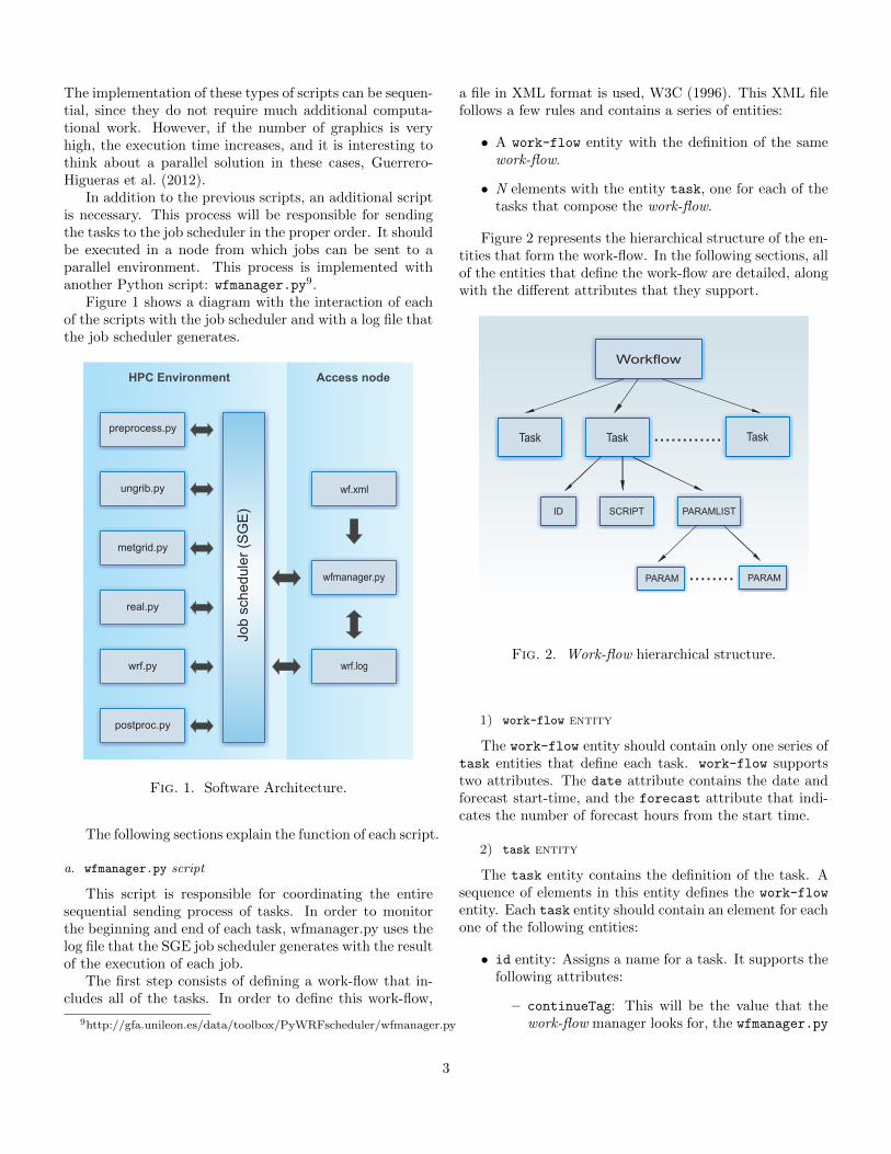
Figure 1 shows a diagram with the interaction of eachof the scripts with the job scheduler and with a log file thatthe job scheduler generates.

wf.xml

wrf.log

wfmanager.py

preprocess.py

ungrib.py

metgrid.py

real.py

wrf.py

postproc.py

Job s

chedule

r (S

GE

)

HPC Environment Access node

Fig. 1. Software Architecture.

The following sections explain the function of each script.

a. wfmanager.py script

This script is responsible for coordinating the entiresequential sending process of tasks. In order to monitorthe beginning and end of each task, wfmanager.py uses thelog file that the SGE job scheduler generates with the resultof the execution of each job.

The first step consists of defining a work-flow that in-cludes all of the tasks. In order to define this work-flow,

9http://gfa.unileon.es/data/toolbox/PyWRFscheduler/wfmanager.py

a file in XML format is used, W3C (1996). This XML filefollows a few rules and contains a series of entities:

• A work-flow entity with the definition of the samework-flow.

• N elements with the entity task, one for each of thetasks that compose the work-flow.

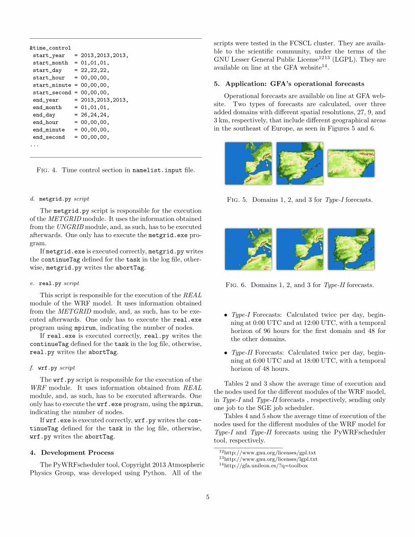
Figure 2 represents the hierarchical structure of the en-tities that form the work-flow. In the following sections, allof the entities that define the work-flow are detailed, alongwith the different attributes that they support.

Workflow

Task Task Task

ID PARAMLIST

PARAM PARAM

SCRIPT

............

........

Fig. 2. Work-flow hierarchical structure.

1) work-flow entity

The work-flow entity should contain only one series oftask entities that define each task. work-flow supportstwo attributes. The date attribute contains the date andforecast start-time, and the forecast attribute that indi-cates the number of forecast hours from the start time.

2) task entity

The task entity contains the definition of the task. Asequence of elements in this entity defines the work-flow

entity. Each task entity should contain an element for eachone of the following entities:

• id entity: Assigns a name for a task. It supports thefollowing attributes:

– continueTag: This will be the value that thework-flow manager looks for, the wfmanager.py

3

script, in the log file created by the SGE jobscheduler, in order to make sure that the taskis executed correctly and that it is possible tocontinue with the the next one.

– abortTag: This will be the value that the work-flow manager looks for, wfmanager.py, in thelog file created by the SGE job scheduler, inorder to make sure that if an error has occurredwhen performing the task, and it is not possibleto continue with the next one.

• script entity: This indicates the script path that thetask executes. It supports the following attributes:

– nodes: Specifies the number of nodes in the pa-rallel calculation environment where the task isexecuted.

– queue: Specifies the execution queue in the pa-rallel calculation environment where the task isexecuted.

• paramlist entity: Contains the list of parametersthat each script needs to carry out a task. Each scriptcontains a different number of parameters. A param

entity is defined for each parameter. Each param ele-ment has a value for each parameter. param supportsthe name attribute that is assigned to each parameter.

wf.xml file shows, available on line at GFA website10

under the terms of the GNU General Public License, thedefinition of a work-flow.

Once the work-flow file is defined in the XML file, awfmanager.py script is executed. wfmanager.py covers theXML file using a parsing process, implemented using theAPI DOM (Document Object Model API) from Python,Python Software Foundation (1990). For each task entitythat appears in the work-flow, wfmanager.py sends a jobto the SGE job scheduler. In order to send jobs to theSGE job scheduler, wfmanager.py uses the qsub command,along with a series of arguments and the script path:

• Working directory (-wd): base directory where thescript works.

• Parallel environment (-pe): number of nodes neededto be reserved to execute each job.

• Name (-N): identifier of job.

• Output (-o): file path that is required to redirect thestandard output.

• (-j): Specifies whether or not the standard errorstream of the job is merged into the standard out-put stream.

10http://gfa.unileon.es/data/toolbox/PyWRFscheduler/wf.xml

• Shell (-S): Shell where the script is executed.

• Queue (-q): queue where the job is sent.

wfmanager.py uses values for the attributes and enti-ties contained in the task entity in order to select the scriptand assign values to the qsub arguments.

b. preprocess.py script

This script does tasks before the execution of the model:

• It is responsible for downloading information in orderto initiate the WRF model. In the GFA executions,the WRF model initiates with the information fromthe Global Forecasting11 (GFS) model.

• It updates data in the model’s configuration files.Specifically, it modifies the date and time of the fore-cast in the namelist.wps and namelist.input files,as shown in Figures 3 and 4.

&share

start_date = ’2013-01-22_00:00:00’,

’2013-01-22_00:00:00’,

’2013-01-22_00:00:00’,

end_date = ’2013-01-26_00:00:00’,

’2013-01-24_00:00:00’,

’2013-01-24_00:00:00’,

...

Fig. 3. Time control section in namelist.wps file.

If both tasks are executed correctly, preprocess.py

writes the continueTag defined for the task in the logfile, otherwise, preprocess.py writes the abortTag.

c. ungrib.py script

This script is responsible for the execution of the UN-GRIB module. First, it should connect information thatallows for the initialization of the model so that UNGRIBcan use it. The same WRF model provides a script witha shell that performs this function: link grib.csh. It isonly necessary to indicate the path and the pattern for thefiles that contain the information needed to initialize themodel. After connecting the entry data, one only has toexecute the ungrib.exe program included in the model’ssoftware.

If ungrib.exe is executed correctly, ungrib.py writesthe continueTag defined for the task in the log file, other-wise, ungrib.py writes the abortTag.

11Carried out by the National Oceanic and Atmospheric Adminis-tration (NOAA).

4

&time_control

start_year = 2013,2013,2013,

start_month = 01,01,01,

start_day = 22,22,22,

start_hour = 00,00,00,

start_minute = 00,00,00,

start_second = 00,00,00,

end_year = 2013,2013,2013,

end_month = 01,01,01,

end_day = 26,24,24,

end_hour = 00,00,00,

end_minute = 00,00,00,

end_second = 00,00,00,

...

Fig. 4. Time control section in namelist.input file.

d. metgrid.py script

The metgrid.py script is responsible for the executionof the METGRID module. It uses the information obtainedfrom the UNGRIB module, and, as such, has to be executedafterwards. One only has to execute the metgrid.exe pro-gram.

If metgrid.exe is executed correctly, metgrid.py writesthe continueTag defined for the task in the log file, other-wise, metgrid.py writes the abortTag.

e. real.py script

This script is responsible for the execution of the REALmodule of the WRF model. It uses information obtainedfrom the METGRID module, and, as such, has to be exe-cuted afterwards. One only has to execute the real.exe

program using mpirun, indicating the number of nodes.If real.exe is executed correctly, real.py writes the

continueTag defined for the task in the log file, otherwise,real.py writes the abortTag.

f. wrf.py script

The wrf.py script is responsible for the execution of theWRF module. It uses information obtained from REALmodule, and, as such, has to be executed afterwards. Oneonly has to execute the wrf.exe program, using the mpirun,indicating the number of nodes.

If wrf.exe is executed correctly, wrf.py writes the con-tinueTag defined for the task in the log file, otherwise,wrf.py writes the abortTag.

4. Development Process

The PyWRFscheduler tool, Copyright 2013 AtmosphericPhysics Group, was developed using Python. All of the

scripts were tested in the FCSCL cluster. They are availa-ble to the scientific community, under the terms of theGNU Lesser General Public License1213 (LGPL). They areavailable on line at the GFA website14.

5. Application: GFA’s operational forecasts

Operational forecasts are available on line at GFA web-site. Two types of forecasts are calculated, over threeadded domains with different spatial resolutions, 27, 9, and3 km, respectively, that include different geographical areasin the southeast of Europe, as seen in Figures 5 and 6.

Fig. 5. Domains 1, 2, and 3 for Type-I forecasts.

Fig. 6. Domains 1, 2, and 3 for Type-II forecasts.

• Type-I Forecasts: Calculated twice per day, begin-ning at 0:00 UTC and at 12:00 UTC, with a temporalhorizon of 96 hours for the first domain and 48 forthe other domains.

• Type-II Forecasts: Calculated twice per day, begin-ning at 6:00 UTC and at 18:00 UTC, with a temporalhorizon of 48 hours.

Tables 2 and 3 show the average time of execution andthe nodes used for the different modules of the WRF model,in Type-I and Type-II forecasts , respectively, sending onlyone job to the SGE job scheduler.

Tables 4 and 5 show the average time of execution of thenodes used for the different modules of the WRF model forType-I and Type-II forecasts using the PyWRFschedulertool, respectively.

12http://www.gnu.org/licenses/gpl.txt13http://www.gnu.org/licenses/lgpl.txt14http://gfa.unileon.es/?q=toolbox

5

Table 2. Execution of Type-I forecasts, sending only onejob to the SGE job scheduler.



REAL 2m3s 128 16 112WRF 45m35s 128 128 0

Table 3. Execution of Type-II forecasts, sending only onejob to the SGE job scheduler.



REAL 1m45s 288 32 256WRF 1h38m15s 288 288 0

6. Conclusion

By executing the WRF model, and sending only onejob to the computing environment, time intervals were ob-served in which there were unused nodes, as seen in Tables2 and 3. By using the PyWRFscheduler, which sends jobsto the computing environment for each module, this didnot occur, since only nodes that were necessary were re-served for each case.

After doing tests, it is important to point out thatthe use of the PyWRFscheduler tool to execute the WRFmodel, guarantees optimal use of the resources in a para-llel computing environment. Thus, its use suggests only asmall upcharge in the total time of execution.

Acknowledgments.

The authors would like to thank the Junta of Castileand Leon for their economic support via the LE176A11-2

Table 4. Execution of Type-I forecasts using PyWRF-scheduler.



REAL 2m33s 16 16 0WRF 46m05s 128 128 0

Table 5. Execution of Type-II forecasts using PyWRF-scheduler.



REAL 1m53s 32 32 0WRF 1h38m32s 288 288 0

project. This study was supported by the following grants:CGL2010-15930; MICROMETEO (IPT-310000-2010-22).

REFERENCES

Guerrero-Higueras, A., E. Garcıa-Ortega, V. Matellan-Olivera, and J. Sanchez, 2012: Procesamiento paralelode los pronosticos meteorologicos del modelo WRF me-diante NCL. Actas de las XXIII Jornadas de ParalelismoJP2012, ISBN: 978-84-695-4471-6., 55–60.

Python Software Foundation, 1990: The document ob-ject model API. http://docs.python.org/2/library/xml.dom.html.

Skamarock, W., J. Klemp, J. Dudhia, D. Gill, D. Barker,W. Wang, and J. Powers, 2005: A description of theadvanced research wrf version 2. NCAR Tech. NoteNCAR/TN-468+STR.

Sun Microsystems, 2002: SunTM ONE Grid Engine Ad-ministration and User’s Guide.

UCAR, 2012: User’s guide for the advanced researchWRF (ARW) modeling system. http://www.mmm.ucar.edu/wrf/users/docs/user guide V3/contents.html.

Unidata, 2012: NetCDF users guide. https://www.unidata.ucar.edu/software/netcdf/docs/user guide.html.

W3C, 1996: Extensible markup language (xml). http://www.w3.org/XML/.

6

schedule wrf model executions in parallel computing ... · schedule wrf model executions in...

Documents