scanning transmission electron microscopy*....

OPTIK 31 Heft 3, 1970

Seite 258-780

Scanning Transmission Electron Microscopy*. I By E. Zeitler a n d M. G. R. Thovnson

R,eceived 16 December 1969

Abstract

shown how this equivalence can be deduced from the consideration of either

Numerical calculations were performed to find the optimum conditions for viewing single atoms, and i t was observed that the contrast increases considerably when the accelerating voltage is raised above 100 KV. Simple analytic expressions are given

Inhal t

Raster-Elektronenmikroskopie in Transmission. Eine Theorie zur Entstehung des Phasenkontrastes im Scanning Transmivvion Electron Microscope ist cntwickelt. Die Beleuchtung wird als koharent angenommen und die unelastische Streuung - vernachlassigt. Die Ergebnisse stimmen mit denen uberein, die man fur denKont'rast in einem konventionellen Elektronenmikroskop erhalt, das unter ahnlichen Bedin- gungen betrieben wird. Diese Aquivalenz beider Mikroskope folgt aus der Vertausch- barkeit von EJektroncnquclle und -detektor.

Die Bildentstehung ist am Beispiel eines unter- und uberfokussierten Phasen- gitters naher dhkutiert. Kumerische R'echnungen werden ausgefuhrt mit dem Ziel, die optimalen Bedingungen zur Abbildung einzelner Atome festzulegen; dabei ergibt sich, daD bei Erhohung der Beschleunigungsspannung iiber 100 kV eine be- trachtliche K~nt~rastzunahrne erzielt werden kann. Einfache analytische Ausdriicke

* Work performed under the auspices of the U.S. Atomic Energy Commission ' Contract AEC AT (11-1)-1721.

Scanning Transmission Electron Microscopy. I

Introduction

The purpose of this paper is to analyse the image formation in a scanning transmission electron niicroscope (STEM) and to compare i t with that in a conventional electron microscope (CEM). By a scanning transmission electron microscope we understand an electron optical device which illuminates small areas of the object under investigation in a time sequence and utilises the

' area by synchronism. In a final step the light distribution is photographed. The definition describes in essence the STEM as developed and perfected

by A. V. Crewe and his collaborators [I.]. I t is clearly different from the conventional scanning electron nlicroscope of the Oatley-Nixon type (SEM)

Since both the CEM and the STEM form images, the connection between the two images in terms of the object and the optical parameters should be established. A very general theory of image formation in the CEM is due to Uyeda [3], who builds up the object with single atoms utilising Scherzer's

and forties by uon Ardenne [7], Boersch [8], and Hillier and Baker [9]. De- pending on the distance between the cross-over of the illumination and the specimen the STEM can be run as a shadow microscope or a diffraction camera. Recording can be done by direct photography or more conveniently by scanning the electron beam after passage through the object. The theories . put forth a t that tinie did not include phase effects, so the treatment of phase effects given in this paper will complement the older theories.

1. Theory of the Scanning Microscope

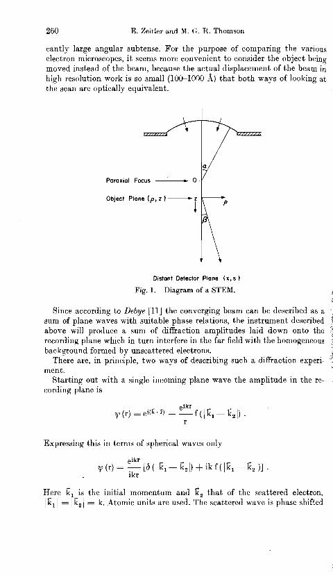
Fig. 1 presents a diagram of a STEM which is in accordance with the general definition given above. We assume a converging, highly coherent electron beam, and place an object a t an axial distance z from the paraxial focus. While the impinging beam is scanned over the object a small detector on axis in the recording plane far distant (30 cm) from the object records the electron current within its cone of angular subtense. The coherent beam may originate from a field emission source [lo]; its features will play a role only when the degree of coherence enters the consideration in section 5. I n sec-

260 E. Ze~tler and M. G. R. Thomson f j

cantly large angular subtense. For the purpose of comparing the various electron microscopes, i t seems more convenient to consider the object being I moved instead of the beam, because the actual displacement of the beam in high resolution work is so small (100-1000 A) that both ways of looking at the scan are optically equivalent.

Distant Detector Plane ( x , s

Fig. 1. Diagram o f a STEM.

Since according to Debye [ I l l the converging beam can be described as a sum of plane waves with suitable phase relations, the instrument described above will produce a sum of diffraction amplitudes laid down onto the recording plane which in turn interfere in the far field with the homogeneous background formed by unscattered electrons.

There are, in principle, two ways of describing such a diffraction experi- ment.

Starting out with a single incoming plane wave the amplitude in the recording plane is

Expressing this in terms of spherical waves only 4 d f

Here El is the initial momentum and z, that of the scattered electron, I gl I = z, I = k. Atomic units are used. The scattered wave is phase shifted

E. Zeitler and M. G. R. Thomson

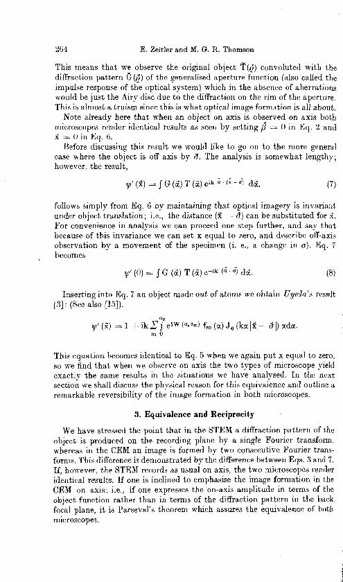
This means that we observe the original object T(@) convoluted with the diffraction pattern GI (6) of the generalised aperture function (also called the impulse response of the optical system) which in the absence of aberrations would be just the Airy disc due to the diffraction on the rim of the aperture. This is almost a truism since this is what optical image formation is all about.

Note already here that when an object on axis is observed on axis both microscopes render identical results as seen by setting B = 0 in Eq. 2 and ,

a = 0 in Eq. 6. Refore discussing this result we would like to go on to the more general '1

case where the object is off axis by 6. The analysis is somewhat, lengthy; i however, the result,

* . * y' (1) = J G (a) T ( 2 ) elk " ' (" - ") dG,

follows simply from Eq. 6 by maintaining that optical imagery is invariant under object translation; i.e., the distance (2 - d ) can be substituted for 2. For convenience in analysis we call proceed one step further, and say that because of this invariance we can set x equal to zero, and describe off-axis

y' (0) = J G (2) T ( 2 ) e-ik 3 dZ.

Inserting into Eq. 7 an object made out of atoms we obtain Uyedn's result 131 : (See also [15]).

a0

yf (2 ) = 1 1- ik J eiw (a, zm) f, (a) J, (ka 12 - 6 I) ada. m 0

This equation becomes identical to Eq. 5 when we again put x equal to zero, so we find that when we observe 011 axis the two types of microscope yield exactly the same results in the situations we have analysed. 111 the next section we shall discuss the physical reason for this equivalence and outline a re~llarkable reversibility of the image formation in both microscopes.

3. Equivalence and Reciprocity

We have stressed the point that in the STEM a diffraction pattern of the object is produced on the recording plane by a single Fourier transform, $ whereas in the CEM an image is formed by two consecutive Fourier trans- forms. This difference is den~onstrated by the difference between Eqs. 3 and 7. ', 1 If, however, the STEM records as usual on axis, the two microscopes render identical results. If one is inclined to emphasise the image formation in the I CEM on axis; i.e., if one expresses the on-axis amplitude in terms of the object function rather than in terms of the diffraction pattern in the back focal plane, i t is Parseval's theorem which assures the equivalence of both microscopes.


Helmholtz [16] which says that a point source a t any point Q producing a certain amplitude in the recording plane a t Y will produce the same amplitude a t Q when placed a t P. Applying this theorem to the CEM, that is, replacing the source of illumination by a small detector and vice versa, we obtain the optical layout of a STEM. This makes clear the necessity for the angular correspondences discussed above. Simple arguments extend this theorem to cover off-axis observation, and finite angles of recording in the STEM, paral- leling our extension of equivalence. We can thus think of a STEM as the equivalent CEM with the directions of motion of the electrons reversed. This reversibility is clear in Fig. 2, where the two microscope diagrams differ only in the direction of the arrows.

The degree of coherence in an illuminating spot depends on the angle of illumination, so care has to be taken when considering the reverse of any microscope for this angle will change. The relatively small illumination angle in a CEM will be transformed into the relatively large one in a STEM. The degree of coherence does not in general reverse. We do not consider the restri~t~ions imposed in detail, although we consider partial coherence in section 5, where we show that for incoherent illumination the reversibility is trivia!. We also do not include effects due to the finite energy spread of the

[IT]. I t was this experimental evidence which suggested the equivale which has been placed on a more formal basis.

of the beam and imaging cathode ray tube, so the transmitted electron be can be processed to gain additional information without destroying

4. Examples with coherent illumination

To classify the various contrast mechanisms and to vitalise the theory of the previous sections, we like to discuss the image formation of a phase grating, which might be thought of as a thin single-crystal, which plays an important role as test specimen to measure the performance of conventional microscopes. The transmission function of such a grating can be written as

Here 6 is the spatial frequency vector, 161 = 2n/A, of the grating with spacing A. A phase angle p, is explicitly introduced, so that it later on can

two, where the illun~ination passes through the specimen before diverging, the diffraction rase.

A. Phuse Grating. Projection, z > 0, With the transmission function given above we find the Fourier transform

-> + 0 1 is smaller than the illuminating aperture oro. In other words the diffraction angle niust stay within the illuminating cone. Expressing G in terms of the aberration function W we optain for the intensity under the angle ,9:

lly'(/?)I2 = 1 + 2a sin [W(p) - 4 W(B + 8) - S W(B - €41 x cos LV + 4 w(p + e) - w(p -011 (12)

+ a2 c0s2 [pl + W ( j + 6) - g W(p - O ) ] .

If p is considered the independent variable, we see that the intensity re- flects faithfully the pl-dependence of the object, neglecting the weak quadrat- ic term. The contrast, however, is reduced by the sine function. By a suitable choice of the experimental parameters /? and z, making the argument

7d of the sine an odd multiple of -, we can assure the contrast to be maximum

2 (negative or positive) :

7d Cs j 2 e 2 = + (2n + 1) - - W(0); n = 0. 1, 2, . . . (13) Z

2

268 E. Zeitler and M. G. R. Thorns011

Experinlentally one would prefer axial (P = 0) to tilted observation (P + 0) f for which the condition, Eq. 13, becomes 4

i

and with i t Eq. 12.

The condition Eq. 14, known as balancing, has been discussed for the CEM by Thon [18] where it is equally pertinent. (See also [19].)

The results derived so far are completely identical to those of a CEM in agreement with the principle of reciprocity. The condition that the observation angle augmented by the "sidebands" remains within the illuminating cone reminds us again of the correspondence between it and the back focal aperture of a CEM.

The well known use of tilted illumination in a CEM, which increases the resolution for a given aperture by adr~litting only one of the first order diffracted beams to interfere with the zero order beam, can be achieved in the STEM by tilted "observation" in a region where only one first order "cone" beats against the zero order cone. The first order cones can be considered to originate from a virtual diffraction spot in the plane of the illumination focus. We come back to this when dealing with real diffraction spots in case B.

As pointed out before in the usual scanning mode the intensity is observed only a t a fixed position (mostly P = 0) while the object TI‘(^) is moved. I t is, however, interesting to discuss the total projected intensity as an image, which can be obtained by either arresting the scan and photograph- ing the intensity distribution on the recording plane, i. e. by converting the STEM to an ordinary projection EM, or by scanning the beam beneath the object across an aperture and displaying the signal in synchronism.

Although we are dealing with diffraction without employing a lens, the intensity distribution iy1(/3) I2resembles the object function whenb is considered the variable. Except for the distortion caused by spherical aberration the argument of the cosine function is linear in P. Since the physical argument is not influenced by this we set Cs and q equal to zero. The modification necessary for a finite C, can be applied later.

We confirm that

8 1 Y' (P) 1' = 1 + 2a sin (kz -)cos (kzP@) + a2 cos2 (kzBf3) t

2

or with the experimental parameters explicitly shown I

1 y 1 (P) 1 ' = I + 2a sin (nN) cos 2 x 1 + a2 c0s2J - . ( A . I 1 Af 2?L 1

The image spacing A' is equal to AM; where the magnification M = s/z results from the projection arrangement. The Fresnel number N equal to A"z1 indicates the number of Fresnel zones as seen from focus which fall within the first spacing; it is the ratio of the angle ,l/z under which one spacing appears to the diffraction angle 1jA.

Eq. 15 certainly does not describe a diffraction pattern but an image. I t is

to the strict phase relation between the diffracted beams so that the original distribution is reproduced after a certa,in path length; i.e.. when the Fresnel number is an odd multiple of 112. The case considered here is simple since we have only one spacing in the grat,ing so that only one Fresnel number influen- ces the contrast, and since we observe a t the infinite Fraunhofer plane. Hence the phase differences are established on the way from the crossover of the illurnination to the object. Cowley and A3foodie [21] and, inore extensi-

since the various Fresnel numbers must be balanced sinlultaneously. Inci- ' dentally for an amplitude grat,ing the Fresnel number must be an even

number, otherwise the sa,me conditions prevail.

k - - ~ ~ ( 3 ) = 1 (c) e(@) ei (e-")' dk

e y ! i ? ( p ) and n ( p ) = e

' lllodified convolution ikzyP

y ~ ~ ( ? ) = e ~ \ T(d) Hjb-7) dd.


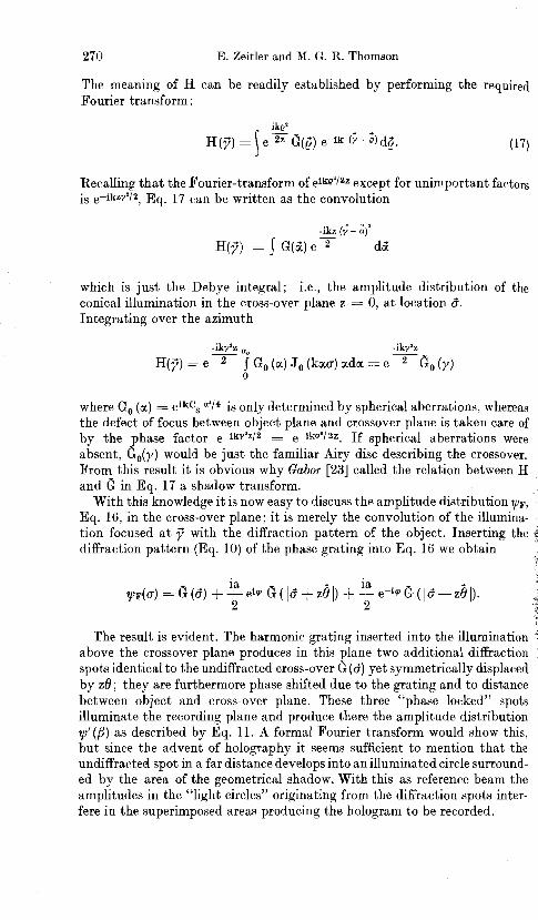
Tl~is description shows that i t is not necessary to distinguish between projection and diffraction, as done here, provided one conceives the projected amplitude as arising from virtual diffraction spots. The proper choice of the sign of defocus z will automatically render the correct phase relations. In short, the grating acts like a Fresnel biprism.

Phase contrast is caused in the CEM by interference between waves which have suffered phase shifts when passing tl~rough the specimen and objective lens. These phase shifts may arise from differences in path lengths, scattering, phaseplates, defocus, or even aberrations. So far we have dealt only with phase contrast, but there is a second contrast mechanism due to the electrons' being preve~lted from reaching the image plane by the objective aperture. This is known as scattering contrast, and will be treated later.

I t is now evident why phase contrast can be observed only if diffracted and undiffracted radiation overlap. This requires that the diffraction angle is snlaller than the illuminating cone, which is nothing but Abbe's resolution criterion. The condition for the focus can be derived by considering the spacing and the extension of the diffraction spots. The extension of the spot, which for an Airy disc is p, = 0.61 l / a , , must clearly be smaller than the distance zf3 = z l / A from the undiffracted spot to avoid overlap in the cross-over plane. This leads t,o the condition that the spacing A must be

In concluding this section we wodd like to mention that the so-called low angle diffraction technique used in CEM is identical to the diffraction mode described in this section. In one version the objective is not engaged, the second condensor is defocuscd such that it forms an image of the source beneath the object. The diffraction pattern is then magnified by the projector system onto the final screen. The method originally introduced by H. Mahl and W. Weitsch, La41 is analysed by R. P. Ferrier and P. T . Murray [25]. In

: their analysis only a geometric optical treatment is given. Since our optical . treatment includes aberrations as well, i t should be Inore generally applicable. In the context of diffraction the experimental parameters are described by the so-called camera constant z l . The focus condition above now states that the product of spot size and spacing must be smaller than the camera con-

272 E. Zeitler and &I. G. It. Thomson

The microscopes chosen for the investigation are essentially practical, using objective lenses which may be constructed with present technology. (We use the term "objective lens" to mean either the usual objective lens in a conventional microscope, or the spot-forming lens in a scanning microscope.) 4 - , * When considering the influence of electron energy i t is necessary to decide ?

how to scale the lens parameters. I t is clearly impractical to retain the same $ values of the focal length, L, and coefficient of spherical aberration, C,, as this would require very high magnetic flux densities a t high energies, so we $ use the more realistic approach of specifying the same peak magnetic field' strengths. We then find that L and Cs are inversely proportional to the electron wavelength, A. We use this method of scaling throughout the paper. I The parameters are based on the lens a t present in use in the high resoiuiion 1 scanning microscope developed by Crewe a t the University of Chicago [I]. i We take LL equal to 0.052 [mm A] and CEA to 0.026 [mm A], corresponding 3 to C, = 0.3 mm a t 20 kV. 4

I n all the computations an infinitely small aperture has been used a t the ' detector. This was done principally to avoid a second complicated integration over the acceptance of the detector, and also because without taking into '

4 consideration the statistical noise in the electron beam in detail it is not clear ; how to choose this acceptance. The operation of phase contrast serves only to 1 redistribute the intensity of the electron beam-over the detector plani, so i the contrast will decrease the greater the recording area. In the limiting case f

we collect the constant total electron flux (as long as the specimen act; only 4 on the phase of the beam). In practice we cannot maximise the contrast since $ both the signal and the signal to noise ratio will decrease. As the noise problem 2 - " is outside the scope of this paper we concentrate on maximum contrast togive :

the ex~erimentalist some ideas of the maximum values he can assume when making the required compromise. Preliminary studies indicate that the contrast will fall only slowly as the acceptance angle is increased, provided that i t remains smaller than the illuminating angle and the atomic screening angle (see Fig. 7).

Lastly, and perhaps of greatest importance, the analysis assumes coherent illumination. The scanning microscope may be treated so as long as the illun~ination half-angle is sufficiently small that the diffraction aberration is greater than the effect of the source size or the chromatic aberration. This condition is essentially met by using a field emission source [lo].

From Eq. 5

and

(10

y' = 1 + ik J' eiW("9 " f (a ) J, (kuo) udu 0 4

= 1 + F say,

ly'I2 = 1 + 2 Re (F) + Re + Im

The lens action is characterised by

274 E. Zoitler and M. G. R. Thomson

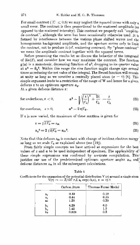
For small contrast ( IC I < 0.5) we may neglect the squared terms with only a small error. The contrast is then proportional to the scattered amplitude (as opposed to the scattered intensity). This contrast we properly call "amplitude contrast", although the term has been occasionally otherwise used. I t is formed by interference between the various phase shifted waves and the homogeneous background amplitude, and the aperture serves only to linlit the contrast, not to produce i t (cf. scattering contrast). By "phase contrastn we mean the amplitude contrast together with the squared terms.

Before presenting the results let us discuss the behavior of the integrand of Re(F), and consider how we may maximise the contrast. The function g (a ) is a monotonic, decreasing function of a2, dropping to its quarter value a t a2 = e02. Within this range the sine function might change sign several times so reducing the net value of the integral. The Bessel function will remaill a t unity as long as we consider a centrally placed atom (o = 0) [6]. This simple argument leads to a restriction of the range of W and hence for a give11 defocus z to an optimum aperture a,. At a given defocus distance z:

21 z for underfocus, z < 0,

for overfocus, z > 0, aa = 2 z/C, .

If z is now varied, the maximum of these maxima is given for i

Note that this defocus z, is constant with change of incident electron energy ' as long as we scale C, as explained above (see [19]).

From fairly simple concepts we have arrived a t expressions for the be values of z and a to be used independent of specimen. The applicabili these simple expressions was confirmed by accurate computation. justifies our use of the predetermined optimum aperture angles a, defocus distances zm in all the subsequent calculations.

Table 1

Coefficients for the expansion of the potential distribution V (r) around a single atom V(r) = - 21137 r Z a j exp(-bjx), x = r/A

I Carbon Atom / Thomas-Fermi Model

0.19 0.10 0.55

a3 1.25 0.35

Scarlr~ir~g Transmission Electron Microscopy. I

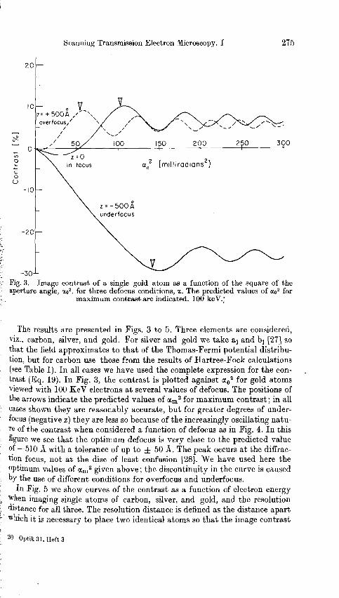
Big. 3. Image contrast of a single gold atom as a function of the square of the aperture angle, mo2, for three defocus conditions, z. The predicted values of ao2 for

maximum contrast are indicated. 100 keV.;

I

! The results are resented in Bigs. 3 to 5 . Three elements are considered, \ viz.. carbon, silver, and gold. For silver and gold n7e take aj and bj [271 so * that the field approximates to that of the Thomas-Fermi potential distribu-

tion, but for carbon use those from the results of Hartree-Bock calculations i, (see Table 1). In all cases we have used the complete expression for the con- . f t ~ a s t (Eq. 19). In Fig. 3, the contrast is plotted against crO2 for gold atoms ; vlewed with 100 KeV electrons at several values of defocus. The positions of

the arrows indicate the predicted values of am2 for maximum contrast; in all f cases shorvn they are reasonably accurate, but for greater degrees of underfocus (negative z) they are less so because of the increasingly oscillating natu- re of the contrast when considered a function of defocus as in Fig. 4. In this

f figure we see that the optimum defocus is very close to the predicted value ! of -510 d with a tolerance of up to f 50 8. The peak occurs a t the diffrac- ; tion focus. not a t the disc of least confusion 1281. We have used here the

L 2

; optimum values of a,2 given above; the discontinuity in the curve is caused a by the use of different conditions for overfocus and underfocus. e In Fig. 5 we show curves of the contrast as a function of electron energy t "hen imaging single atoms of carbon, silver, and gold, and the resolution J distance for all three. The resolution distance is defined as the distance apart i which it is necessary to place two identical atoms so that the image contrast

20 Optik 31, Heft 3


Underfocus Over focus

- - - I 0

0

- 3 0

Fig. 4. Image contrast of a single gold atom as a function of defocus, z, a t optinlum i aperture angles, ao. Different criteria are used to set ao for overfocus and underfocus. .

100 keV. (Eq. 22 and 23)

Accelerating Potential [vol ts]

Fig. 5. Image contrast of single carbon, silver, and gold atoms, and the resolution distance R for all three, as functions of the beam accelerating voltage. The aperture angle and defocus are optimal (see Eq. 24 and 25) and the coefficient of spherical

aberration of the objective lens has been scaled.

j tions in the resolution distance between the elements were less than 10/0, the ; accuracy of the computation. At this point is important to realise tha t we

high voltage electron microscopes. As a spot check the contrast and image profile half-width in the image of a gold atom were evaluated for one of the examples used by Eisenhandler and Siegel [fi]. The example chosen was the 100 KeV lens wit'h C, = 0.035 mm and the given values of z and a,; bhe agreement of both parameters was to within 5%. The observed difference is presumably caused by the different atomic potential models used, and i t is encouraging to see tha t a n analytic formulation gives agreement this good.

Although the calculations are straightforward, they require a computer, and they have the disadvantage common to all numerical results of not showing the influence of the various parameters as readily as an analytic expression. We therefore derived a simple formula for the amplitude contrast on axis by making additional approximations, and showed by means of the extensive numerical material tha t the inherent errors do not exceed ten per

: cent. This value seems accepbable on account of uncertainties in the experimental parameters.

amz .C=-kq 5 g(a)d(a2) .

h 0 ;


taking g(a) to be constarlt and performing the remaining integration of the sine function. This leads for the balanced case to the tabulated Fresnel inte- grals [30] :

q ( p ) = C ( 1 ) c o s p + S ( l ) s i n p

= 0.779 cos y + 0.438 sin y.

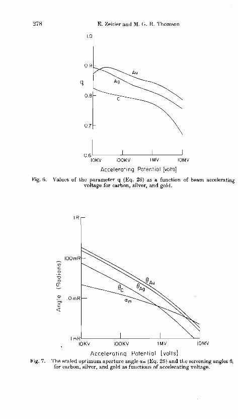
we can now understand more fully the variations of q in Fig. 6. The scattering phase angle a, is approximately equal t o ZJ3/137k, so for carbon (low Z) i t is unimportant; however our approach is not quar~titatively valid above 1 MeV where 0, drops below a, (see Fig. 7). Therefore we can expect a value of q close to q(0) = 0.779 for energies up to 1 MeV, and a smaller value beyond. For gold (high Z) the larger value of y will cause an increase in q above q(0) which will lessen as the energy is increased, and begin t o fall more quickly on account of the decrease in 8 , as the energy approaches 10 MeV. At 20 keV, q will be near the maximum possible value of 0.895, corresponding t o p, = 0.51.

Three important corlclusions can be drawn from these results. The ideal

, amplitude is phase shifted by an additional n / 2 uniformly across the ! aperture independent of the scattering angle. The real q-values above lie ; . quite close to unity, and show how difficult i t is to improve upon such use of ?..

i::. the microscope. i :

C 0 0

0 I L IOKV IOOKV 1MV lOMV

Accelerat ing Potent ia l [ vo l t i ] 8. The amplitude contrast for a silver atom, A; the contrast predicted by

Eri. 27 with q : 0.85, B; and scaled values of the beam energy E and Elk.

E. Zeitler and 31. C:. R. Tllomson

Phase shifts must be introduced to obt,ain an image of a phase object. Tile means a t hand are defocus and spherical aberration. Each on its own introdu- ces phase shifts which are angle dependent, and thus undesirable. Together, however, they can be balanced so that their action becomes that of a phase plate in a light niicroscope [13]. Spherical aberration is beneficial in producing this quasi-uniform phase plate (q == 0.85 instead of q = 1) ; its disadvantage comes from restricting uo2 to v1K These considerations show that experi- ments wit,h actual phase plates [32], which are very difficult to construct, cannot improve significantly on a real microscope with balanced spherical aberration. In a strictly aberration-free microscope, phase plates could cornplernent the phase-shift p, (a) inherent in the scattering process [33], but even without such aid the phase shift introduced by a defocus of 1/uo2 gives a q-value of 0.637.

Third, to make the energy dependence of the contrast more explicit expand the logarithm term in Eq. 27 and find that if we scale Cs and u, as usual, then the contrast is proportional to E and not Elk as has been stated. The expansion of the logarithm is only valid as long as

uo < bj 8, for all j

and this condition usually breaks down a t around 100 keV. At higher energies the logarithm cannot be expanded and the contrast increases less quickly than expected, but always faster than the dependence Elk. At no time does tlie contrast decrease significantly, but a t low energies (where E m 1) i t remains constant (see Fig. 8).

Finally we attempted to represent our calc,ulated resolution by a simple expression. Guided by the diffraction aberration

0.61 1 6 =- = 0.44 1314 a Csl14 urn

we found the results to show the sarne dependence, narnely

R = q 13/4Cs'/4

with q = 0.6 instead of the ideal value of 0.44. This is substantially correct over the range from 10 keV - 10MeVand has been given by Scherzer [4]. If we scale C, as above we find

showing a dependence on 1fr [34].

Scanning Transmission Electron Microscopy. 11*

By E. Zeitler and ,If. G. R. Thornsoya

Department of Physics and Enrico Fermi Institute, theuniversity of Chicago

Received 16 December 1969 Z t

5. Partial Coherence

So far we have dealt only with the case of completely coherent illu~nina- tion. Since one object point, however, is illuminated from many in the source, the diffraction patterns produced by the various source points might be laterally displaced and hence the composite appears with less contrast. The angle of the illumination determines the degree to which the visibility of

: these patterns decreases. If the visibility is zero we speak of complete incohe- rence, and between the two extreme cases we use the concept of the degree of

r , partial coherence. i.' The degree of coherence pl, between two object points depends, as shown , by Hopkin,s [35], on their separation el:, and their half-angle of illumination y

: In the general case this factor multiplies the cross term which appears when the amplitudes are squared to give the ~ntensity. That means, in order to retam the cross tern1 (the amplitude contrast) lplz 1 should be close t o unity. '

1 Custon~ari l~ one is corlterlt with Jp,, J = 0.88, which occurs when the argument kyplz is equal to unlty, or, in other words, the disc with radius

1 . : 1s alnlost coherently illuminated. i The lateral coherence length e, is t o be compared with both the size of the

source image Q , and the separation of the deta,il in which we are interested e l , . The condition for obtaining coherent operation and achieving phase

{ contrast is tha t the illumination must be almost coherent over a distance a t j least as great as the detail; the method of achieving this coherence differs in

the two types of microscope.

* Part I: Optik 31 (1970) 269


In both cases the detail el, is the same, but in the STEM we illuminate an area equal in size to this detail, and thus we require that the whole illuminating spot be coherent. This is so if e, 2 e,; i. e. if

0.161 - 2 e s

Y

The illuminating angle y is equal to the objective aperture angle a, so our condition becomes

0.161 - 2 es

a0

As an example, if we use a, = 0.018 radians a t 20 keV, then es < 0.76 ,i. In a CEM the source size is very much larger as we illuminate all of the

field of view simultaneously. If we are dealing with the imaging of single atoms we can take el, equal to the resolution distance, approximately l/a,. since we are not interested in interference effects between points separated by greater amounts. The illumination angle is Po, so we obtain

0.161 1 -2-

Pt a o

1. e.

Po < 0.16 a,.

To quote the same example as above, if a, is 0.018 radians a t 20 keV, then Po < 0.003. If we are interested in detail of greater extent, as when we are imaging periodic gratings, then e,, will be very much greater and Po smaller. See, for example, [26].

This consideration demonstrates one of the principal differences between a CEM and a STEM. When we reverse the nlicroscopes, the objective aperture angles remain the same size, and the detector angle in the STEM is seen to correspond to the illumination angle in the CEM. However, the illumination angle y is very different; fortunately the coherence criteria are also different so we can obtain coherence by taking the appropriate action in either case. In the STEM the problem is to produce a very small source image, of the order of 1 A, and in the CEM to produce a very small illumination angle. of the order of a few milliradians.

If we write the amplitude due to a composite object (Eq. 5) as

yf = 1 +ZFm

then the intensity, taking account of partial coherence, becomes

( Y' / ' = 1 + 2 Re ( Z p o m F m ) + Z Z p m n F m Fn. 4

362 E. Zeitler and M. G. R. Thomson

acceptance angle of the recorder, both in units of O,, the fraction 1 - k ex- cluded by the aperture a, is

This result confirms the reversibility of both microscopes for the incoherent case. If PoZ < 1 is considered in CEM, we regain the usual expression [36]

We now define contrast as the fractional change in intensity a t the recorder when the specimen is placed in the beam. This definition is consistent with that used above in the coherent illumination treatment, section 4 C. Let us assume that m is the mean number of impacts made by each electron while passing through the specimen. From Eq. 30 above the contrast C is given by

where y 2 = aO2 when Po2 > ao2

= Po2 when ao2 > Po2.

I t is assumed that a negligible number of electrons are scattered by more than one atom, so we must require rn 4 1. The expression is symmetric in ao2 and Po2, and is presented topographically in Pig. 9.

I t is clear from this figure that for any given value of Po the best contrast is obtained when a, = Po. Further, the maximum possible contrast is given when a, and Po are as small as possible. However, consideration of the statistical noise in the electron beam prohibits too small a value of either a, or 8,. and usually the optinlum signal to noise ratio occurs a t large values of both parameters. From these considerations the best operating conditions u-ould seem to be a large value of Po, and an equal or slightly smaller value of a,.

2. The second part, S', of the double sum depends not only on the degree of coherence but also on the phase relations determined by the internal order of the specimen ("structural coherence"). Consequently we call S' the partial]! coherent intensity.

If there w'ere no internal order and p,, = 1, the specimen could be described as having a uniform refractive index within its geonietric bounds, as


distribution for carbon black. He uses X-rays and hence a large sample for his study. In conventional electron diffraction the sample is still large enough that the results for both types of radiation agree [38]. Their result can be described as the average deviation of density from the bulk density as a function of distance from an arbitrary atom over the total volume. The STEM, however, responds to the actual density of each small sample. The usual radial distribution can be obtained only by averaging over all the measured samples, for example by means of optical diffraction of the picture obtained. Only if enough spots are measured will the deduced radial distribution agree with that of the large sample. Since averaging essentially reduces the amount of data the STEM provides more information by averag- ,

ing over a smaller sample. The greater amount of information could be expressed, for example, as the standard deviation from the averaged radial distribution.

If the specimen is a crystal, Bragg reflections can transfer intensit? outside of the cone of acceptance. (The sum S pertains then only to atoms on j planes fulfilling t'he Bragg condition.) Based on the work with converging illumination by Kossel and Mollenstedt [39], Davidson and Hillier [4O] g' ~ v e an extensive discussion of the diffraction images of microcrystallites observed in their diffraction-projection electron microscope. Since, as pointed out be-

serred in the STEM.

6. Summary and Conclusions

1. We have shown that the conventional electron microscope (CEM) and

the various modes and proved them to be in accordance with reciprocity. ' 2. The results are used to predict the quality of the images of phase gratings

and single atonis. The optimum conditions for viewing single atoms are derived, and the expected phase contrast given for different incident electron : energies. Increasing the energy is seen to yield both better resolution distance

instruments, the illumination angles will generally be very different. Optical-

4. The extent of the sample illuminated in a CEM is large compared to the resolution, whereas in a STEM i t is in the order of the resolution. In the diffraction mode deviations from the mean nearest neighbour order from sample to sample produce effects in the STEM which cannot occur in the

Scanning Transmission Electron Microscopy. I1

5. Energy selection can be carried out in the STEM without destroyiilg the imaging process, thus offering a simple way of making use of the inelastically scattered electrons. This could be extended to use a whole array of recorders, each one recording one of the various groups of scattered or unscattered electrol~s, and so bringing out special features of the specimen as contrast niiips [41].

6. The STEM is essentially more simple than the CEM because the image is coi~structed by the synchronism of the scaus over the specimen and the

,: viewing screen. An increase in magnification can be achieved by decreasing

f . only be transformed with difficulty into an electronic signal. Advanced iniage ! . : improvement techniques can only be accomplished by electronic means, so

to this end flying spot microdenvitometers are coming into use as interphases between the output of the CEM (the micrograph) and the data handling

\ . device (a computer). This is not necessary for the STEM. So, if all the optical - j features of both inicroscopes were just equal, the STEM can be seen as a : con~biilation of a CEM with an on-line microdensitometer avoiding two

Acknowledgements

: The authors wish to express their thanks to Professor Albert V. Crewe and the members of his group for invaluable advice and encouragement through-

: out this work.

References

scanning transmission electron microscopy*....

Documents