scalable column generation models and ......abstract scalable column generation models and...
TRANSCRIPT

SCALABLE COLUMN GENERATION MODELS AND
ALGORITHMS FOR OPTICAL NETWORK PLANNING
PROBLEMS
Hai Anh Hoang
A thesis
in
The Department
of
Computer Science
Presented in Partial Fulfillment of the Requirements
For the Degree of Doctor of Philosophy
Concordia University
Montreal, Quebec, Canada
August 2014
c© Hai Anh Hoang, 2014

Concordia UniversitySchool of Graduate Studies
This is to certify that the thesis prepared
By: Mr. Hai Anh Hoang
Entitled: Scalable Column Generation Models and Algorithms for
Optical Network Planning Problems
and submitted in partial fulfillment of the requirements for the degree of
Doctor of Philosophy (Computer Science)
complies with the regulations of this University and meets the accepted standards
with respect to originality and quality.
Signed by the final examining commitee:
Chair
Dr. Didier Colle, External Examiner
Dr. Brigitte Jaumard, Thesis Supervisor
Dr. Jaroslav Opatrny, Examiner
Dr. Hovhannes A. Harutyunyan, Examiner
Dr. John Xiupu Zhang, Examiner
ApprovedChair of Department or Graduate Program Director
20
Dr. Christopher W. Trueman, Interim Dean
Faculty of Engineering and Computer Science

Abstract
Scalable Column Generation Models and Algorithms for Optical
Network Planning Problems
Hai Anh Hoang, Ph.D.
Concordia University, 2014
Column Generation Method has been proved to be a powerful tool to model and
solve large scale optimization problems in various practical domains such as operation
management, logistics and computer design. Such a decomposition approach has been
also applied in telecommunication for several classes of classical network design and
planning problems with a great success.
In this thesis, we confirm that Column Generation Methodology is also a powerful
tool in solving several contemporary network design problems that come from a rising
worldwide demand of heavy traffic (100Gbps, 400Gbps, and 1Tbps) with emphasis on
cost-effective and resilient networks. Such problems are very challenging in terms of
complexity as well as solution quality. Research in this thesis attacks four challenging
design problems in optical networks: design of p-cycles subject to wavelength conti-
nuity, design of dependent and independent p-cycles against multiple failures, design
of survivable virtual topologies against multiple failures, design of a multirate opti-
cal network architecture. For each design problem, we develop a new mathematical
models based on Column Generation Decomposition scheme.
Numerical results show that Column Generation methodology is the right choice to
deal with hard network design problems since it allows us to efficiently solve large scale
network instances which have been puzzles for the current state of art. Additionally,
the thesis reveals the great flexibility of Column Generation in formulating design
problems that have quite different natures as well as requirements.
Obtained results in this thesis show that, firstly, the design of p-cycles should
be under a wavelength continuity assumption in order to save the converter cost
since the difference between the capacity requirement under wavelength conversion
vs. under wavelength continuity is insignificant. Secondly, such results which come
from our new general design model for failure dependent p-cycles prove the fact that
iii

failure dependent p-cycles save significantly spare capacity than failure independent
p-cycles. Thirdly, large instances can be quasi-optimally solved in case of survivable
topology designs thanks to our new path-formulation model with online generation of
augmenting paths. Lastly, the importance of high capacity devices such as 100Gbps
transceiver and the impact of the restriction on number of regeneration sites to the
provisioning cost of multirate WDM networks are revealed through our new hierar-
chical Column Generation model.
iv

Acknowledgments
First and foremost, I would like to express my sincerest and earnest gratitude to
my supervisor, Dr. Brigitte Jaumard for her guidance, support, and enthusiasm
throughout my PhD study at Concordia University. Her immense knowledge, helpful
suggestions and comments as well as encouragements make this research possible. I
am grateful to her for the valuable time she puts in the discussions on my research
projects. I would like to thank to Dr. Christine Tremblay for her suggestions and
close collaboration on chapter 7.
I deeply appreciate my thesis committee for their prompt evaluation and com-
ments. Their valuable feedbacks and questions improve my thesis work. I also would
like to thank my lab mates for the delightful environment that they have provided
me with.
Last but not least, I would like to extend the deepest gratitude to my dear family
for their moral support and inspiration. I am greatly indebted to my mother and
my brother for their unconditional encouragement and love and to my fiance for her
understanding, patience, and care during all these years.
v

Contents
List of Figures x
List of Tables xi
List of Acronyms xii
List of Publications xiv
1 Introduction 1
1.1 Background . . . . . . . . . . . . . . . . . . . . . . . . . . . . . . . . 1
1.2 Research projects . . . . . . . . . . . . . . . . . . . . . . . . . . . . . 3
1.2.1 Design of p-cycles subject to wavelength continuity . . . . . . 4
1.2.2 Design of dependent and independent p-cycles against multiple
failures . . . . . . . . . . . . . . . . . . . . . . . . . . . . . . . 5
1.2.3 Design of survivable virtual topologies against multiple failures 6
1.2.4 Design of a multirate optical network architecture . . . . . . . 7
1.3 Contributions . . . . . . . . . . . . . . . . . . . . . . . . . . . . . . . 8
1.4 Plan of thesis . . . . . . . . . . . . . . . . . . . . . . . . . . . . . . . 10
2 Optical network background 11
2.1 Equipment and physical aspects . . . . . . . . . . . . . . . . . . . . . 11
2.2 Cross-layer design . . . . . . . . . . . . . . . . . . . . . . . . . . . . . 14
2.3 Survivability and main protection schemes . . . . . . . . . . . . . . . 15
2.4 Column generation methodology . . . . . . . . . . . . . . . . . . . . . 18
2.4.1 A single pricing CG algorithm . . . . . . . . . . . . . . . . . . 18
2.4.2 A multiple pricing CG algorithm . . . . . . . . . . . . . . . . 19
vi

3 Literature review 21
3.1 The RWA problem with p-cycles and wavelength conversion . . . . . 21
3.2 Multiple link failures in WDM networks . . . . . . . . . . . . . . . . 24
3.3 Survivable logical topology design . . . . . . . . . . . . . . . . . . . . 27
3.4 Multirate cross-layer optical network design . . . . . . . . . . . . . . 30
3.5 Conclusion . . . . . . . . . . . . . . . . . . . . . . . . . . . . . . . . . 33
4 Design of p-cycles subject to wavelength continuity 34
4.1 Problem statement . . . . . . . . . . . . . . . . . . . . . . . . . . . . 34
4.2 Notion of configuration . . . . . . . . . . . . . . . . . . . . . . . . . . 36
4.3 Definitions and notations . . . . . . . . . . . . . . . . . . . . . . . . . 37
4.4 Decomposition model for p-cycles with wavelength continuity assumption 39
4.4.1 Master problem . . . . . . . . . . . . . . . . . . . . . . . . . . 39
4.4.2 Pricing problem . . . . . . . . . . . . . . . . . . . . . . . . . . 40
4.5 Decomposition model for p-cycles without wavelength continuity as-
sumption . . . . . . . . . . . . . . . . . . . . . . . . . . . . . . . . . . 42
4.5.1 Master problem . . . . . . . . . . . . . . . . . . . . . . . . . . 42
4.5.2 Working path pricing problem . . . . . . . . . . . . . . . . . . 42
4.5.3 p-Cycle pricing problem . . . . . . . . . . . . . . . . . . . . . 43
4.6 Decomposition model for FIPP p-cycles with wavelength continuity
assumption . . . . . . . . . . . . . . . . . . . . . . . . . . . . . . . . 43
4.7 Decomposition model for FIPP p-cycles without wavelength continuity
assumption . . . . . . . . . . . . . . . . . . . . . . . . . . . . . . . . 45
4.7.1 Master problem . . . . . . . . . . . . . . . . . . . . . . . . . . 45
4.7.2 FIPP p-cycles pricing problem . . . . . . . . . . . . . . . . . . 46
4.8 Numerical results . . . . . . . . . . . . . . . . . . . . . . . . . . . . . 47
4.9 Conclusion . . . . . . . . . . . . . . . . . . . . . . . . . . . . . . . . . 50
5 Design of dependent and independent p-cycles against multiple fail-
ures 51
5.1 Definitions and notations . . . . . . . . . . . . . . . . . . . . . . . . . 52
5.2 FDPP p-cycle decomposition model . . . . . . . . . . . . . . . . . . . 55
5.2.1 Master problem . . . . . . . . . . . . . . . . . . . . . . . . . . 55
5.2.2 Pricing problem . . . . . . . . . . . . . . . . . . . . . . . . . . 55
vii

5.3 Solution enhancements . . . . . . . . . . . . . . . . . . . . . . . . . . 57
5.3.1 Speed up pricing problem . . . . . . . . . . . . . . . . . . . . 57
5.3.2 Memory management . . . . . . . . . . . . . . . . . . . . . . . 58
5.4 Insights into the proposed model . . . . . . . . . . . . . . . . . . . . 59
5.4.1 Compare with the previously proposed model . . . . . . . . . 59
5.4.2 As a node protection framework . . . . . . . . . . . . . . . . . 60
5.4.3 An example where FDPP solution exists but FIPP solution
does not . . . . . . . . . . . . . . . . . . . . . . . . . . . . . . 61
5.5 Numerical results . . . . . . . . . . . . . . . . . . . . . . . . . . . . . 62
5.5.1 Network and data instances . . . . . . . . . . . . . . . . . . . 63
5.5.2 Performance of the FDPP p-cycle model: single link failure . . 63
5.5.3 Performance of the FDPP p-cycle model: dual link failure . . 64
5.5.4 FDPP p-cycle model: node protection . . . . . . . . . . . . . 66
5.5.5 FDPP p-cycle model: triple & quadruple link failure . . . . . 67
5.6 Conclusion . . . . . . . . . . . . . . . . . . . . . . . . . . . . . . . . . 68
6 Design of survivable virtual topologies against multiple failures 69
6.1 The decomposition model . . . . . . . . . . . . . . . . . . . . . . . . 73
6.1.1 Definitions and notation . . . . . . . . . . . . . . . . . . . . . 73
6.1.2 Variables . . . . . . . . . . . . . . . . . . . . . . . . . . . . . . 75
6.1.3 Master problem . . . . . . . . . . . . . . . . . . . . . . . . . . 76
6.1.4 Pricing problem . . . . . . . . . . . . . . . . . . . . . . . . . . 78
6.1.5 Solving multi-level ILP objective . . . . . . . . . . . . . . . . 80
6.1.6 Computing the required spare capacity for a successful IP restora-
tion . . . . . . . . . . . . . . . . . . . . . . . . . . . . . . . . 81
6.2 Numerical results . . . . . . . . . . . . . . . . . . . . . . . . . . . . . 82
6.2.1 Data instances . . . . . . . . . . . . . . . . . . . . . . . . . . 82
6.2.2 Transport capacity and link dimensioning . . . . . . . . . . . 83
6.2.3 Quality of solutions . . . . . . . . . . . . . . . . . . . . . . . . 86
6.2.4 Networking performances . . . . . . . . . . . . . . . . . . . . . 87
6.3 Conclusion . . . . . . . . . . . . . . . . . . . . . . . . . . . . . . . . . 89
7 Design of a multirate optical network architecture 91
7.1 Problem description . . . . . . . . . . . . . . . . . . . . . . . . . . . . 92
viii

7.2 Cost model . . . . . . . . . . . . . . . . . . . . . . . . . . . . . . . . 94
7.3 Decomposition model . . . . . . . . . . . . . . . . . . . . . . . . . . . 95
7.3.1 Definitions and notations . . . . . . . . . . . . . . . . . . . . . 96
7.3.2 Master model . . . . . . . . . . . . . . . . . . . . . . . . . . . 98
7.3.3 Pricing I: generation of wavelength configurations (γ) . . . . . 99
7.3.4 Pricing II: generation of multi-hop path configuration (π) . . . 100
7.3.5 Adaptation to undirected model . . . . . . . . . . . . . . . . . 101
7.4 Solution of the models . . . . . . . . . . . . . . . . . . . . . . . . . . 101
7.5 Numerical experiments . . . . . . . . . . . . . . . . . . . . . . . . . . 102
7.5.1 Data instances . . . . . . . . . . . . . . . . . . . . . . . . . . 103
7.5.2 Impact of traffic volume and physical constraints on CAPEX . 107
7.6 Conclusion . . . . . . . . . . . . . . . . . . . . . . . . . . . . . . . . . 113
7.7 Future work . . . . . . . . . . . . . . . . . . . . . . . . . . . . . . . . 113
8 Conclusion and future works 115
8.1 Conclusion . . . . . . . . . . . . . . . . . . . . . . . . . . . . . . . . . 115
8.2 Future works . . . . . . . . . . . . . . . . . . . . . . . . . . . . . . . 116
Bibliography 118
ix

List of Figures
2.1 Multiplexer and demultiplexer. . . . . . . . . . . . . . . . . . . . . . 12
2.2 A model of optical switch where a wavelength is either bypassed, con-
verted, added or dropped . . . . . . . . . . . . . . . . . . . . . . . . . 13
2.3 A single pricing CG algorithm . . . . . . . . . . . . . . . . . . . . . . 19
2.4 A multiple pricing CG algorithm . . . . . . . . . . . . . . . . . . . . 20
4.1 An unfeasible protection solution . . . . . . . . . . . . . . . . . . . . 35
4.2 Configuration decomposition of a WDM network . . . . . . . . . . . . 36
5.1 ILP & column generation algorithm . . . . . . . . . . . . . . . . . . . 58
5.2 A backup cycle . . . . . . . . . . . . . . . . . . . . . . . . . . . . . . 60
5.3 A node failure . . . . . . . . . . . . . . . . . . . . . . . . . . . . . . . 61
5.4 Transformation of a node failure into a link failure . . . . . . . . . . . 61
5.5 FDPP vs FIPP . . . . . . . . . . . . . . . . . . . . . . . . . . . . . . 62
5.6 Number of selected/generated configurations . . . . . . . . . . . . . . 65
5.7 R2 ratio vs. capacity redundancy . . . . . . . . . . . . . . . . . . . . 66
6.1 A survivable mapping example . . . . . . . . . . . . . . . . . . . . . . 70
6.2 Explain why redundancy ratio is a significantly large number. . . . . 88
7.1 A simple multirate optical network . . . . . . . . . . . . . . . . . . . 94
7.2 Outline of the solution process . . . . . . . . . . . . . . . . . . . . . . 102
7.3 Traffic demand distribution . . . . . . . . . . . . . . . . . . . . . . . 105
7.4 US-24 network . . . . . . . . . . . . . . . . . . . . . . . . . . . . . . . 106
7.5 Average of transceiver percentages of 750km, 1500km and 3000km . . 107
7.6 Average of transceiver percentages of 10Gbps, 40Gbps and 100Gbps . 109
7.7 Comparison of percentages of transceivers grouped by bit-rate that
is made between the case of maximum 12 regenerable sites and of
maximum 24 regenerable sites . . . . . . . . . . . . . . . . . . . . . . 111
7.8 Cost comparison between different amount of maximum regenerable sites112
x

List of Tables
3.1 Characteristics of studies in the static p-cycle RWA problem . . . . . 24
3.2 Characteristics of studies in multiple link failures . . . . . . . . . . . 27
3.3 Characteristics of studies in survivable virtual topology . . . . . . . . 29
3.4 Characteristics of studies in multirate cross-layer optical network design 32
4.1 Characteristics of the data sets tested with the p-cycle model . . . . . 47
4.2 Results obtained under a joint-optimization scheme with/without wave-
length conversion capacity for the p-cycle model . . . . . . . . . . . . 48
4.3 Results obtained under a joint-optimization scheme with/without wave-
length conversion capacity for the FIPP p-cycle model . . . . . . . . 49
5.1 Description of Network Instances . . . . . . . . . . . . . . . . . . . . 63
5.2 Comparison of FIPP p-cycle models vs. FDPP p-cycle models. . . . . 64
5.3 Accuracy of the Solutions . . . . . . . . . . . . . . . . . . . . . . . . 65
5.4 Node protection solutions . . . . . . . . . . . . . . . . . . . . . . . . 67
5.5 High order link protection scenario description . . . . . . . . . . . . . 67
5.6 Higher order link protection scenario . . . . . . . . . . . . . . . . . . 68
6.1 Routing bandwidth and additional bandwidth . . . . . . . . . . . . . 72
6.2 Network Topologies . . . . . . . . . . . . . . . . . . . . . . . . . . . . 83
6.3 Performance of the decomposition model . . . . . . . . . . . . . . . . 84
6.4 Existence and dimensioning of a survivable logical topology (single-link
failures) . . . . . . . . . . . . . . . . . . . . . . . . . . . . . . . . . . 85
6.5 Multiple failure set scenarios . . . . . . . . . . . . . . . . . . . . . . . 88
6.6 Existence and dimensioning of a survivable logical topology (multiple-
link failures & |Vp| = 1/2|Vl|) . . . . . . . . . . . . . . . . . . . . . . 89
7.1 Cost model (MTD = Maximum Transmission Distance). . . . . . . . 95
7.2 Traffic load vs. co . . . . . . . . . . . . . . . . . . . . . . . . . . . . . 104
7.3 Statistics of the percentage average . . . . . . . . . . . . . . . . . . . 108
xi

List of Acronyms
CG Column Generation
LP Linear Programming
ILP Integer Linear Programming
MP Master Problem
RMP Restricted Master Problem
OC Optical Carrier
Gbps Gigabits per second
Tbps Terabits per second
WDM Wavelength-Devision Multiplexing
OXC Optical Cross Connect
RWA Routing Wavelength Assignment
IP Internet Protocol
LSP Label Switching Path
MPLS Multi-Protocol Label Switching
FDPP Failure-Dependent Path Protection
FIPP Failure-Independent Path Protection
SRLG Shared Risk Link Group
xii

MTR Maximum Transmission Reach
CAPEX Capital Expenditure
OPEX Operating Expense
xiii

List of Publications
Manuscripts to be submitted
[Jaumard and Hoang Hai Anh] Brigitte Jaumard and Hoang Hai Anh. Design and
Dimensioning of Logical Survivable Topologies against Multiple Failures.
In Journal of Optical Communications and Networking.
[Hoang Hai Anh and Jaumard] Hoang Hai Anh and Brigitte Jaumard. Design of a
multirate optical network architecture. In Journal of Optical Communications
and Networking.
Published manuscripts
[Jaumard et al., 2013] Brigitte Jaumard, Hoang Hai Anh, and Do Trung Kien. Robust
FIPP p-cycles against dual link failures. Telecommunication Systems, pages
1–12, 2013.
[Jaumard and Hoang Hai Anh, 2013] Brigitte Jaumard and Hoang Hai Anh. Design
and Dimensioning of Logical Survivable Topologies Against Multiple
Failures. In Journal of Optical Communications and Networking, pages 23–36,
2013.
xiv

[Jaumard et al., 2012] Brigitte Jaumard, Hoang Hai Anh, and Bui Nguyen Minh. Path
vs. Cutset approaches for the design of logical survivable topologies. In
IEEE International Conference on Communications (ICC), pages 3061–3066, 2012.
[Jaumard and Hoang Hai Anh, 2012] Brigitte Jaumard and Hoang Hai Anh. Design
of Survivable IP-over-WDM Networks (invited). In The Fourth Interna-
tional Conference on Communications and Electronics, pages 13–18, 2012.
[Hoang Hai Anh and Jaumard, 2011a] Hoang Hai Anh and Brigitte Jaumard. RWA
and p-Cycles. In Ninth Annual Communication Networks and Services Research
Conference (CNSR), pages 195–201, May 2011a.
[Hoang Hai Anh and Jaumard, 2011b] Hoang Hai Anh and Brigitte Jaumard. De-
sign of p-Cycles under a Wavelength Continuity Assumption. In IEEE
International Conference on Communications (ICC), pages 1–5, June 2011b.
[Hoang Hai Anh and Jaumard, 2011c] Hoang Hai Anh and Brigitte Jaumard. A New
Flow Formulation for FIPP p-Cycle Protection subject to Multiple Link
Failures (Best Paper Award). In 3rd International Congress on Ultra Modern
Telecommunications and Control Systems and Workshops (ICUMT), pages 1–7,
October 2011c.
[Jaumard et al., 2011] Brigitte Jaumard, Hoang Hai Anh, and Bui Nguyen Minh. Using
decomposition techniques for the design of survivable logical topologies.
In 5th International Conference on Advanced Networks and Telecommunication
Systems (ANTS), pages 1–6, December 2011.
xv

Chapter 1
Introduction
1.1 Background
The growth rate of traffic over the global IP backbone network is expected to be
increased by approximately a factor of 12 over next decade [Korotky, 2012; Cisco,
2013]. To answer to the significant traffic demand that is coming, a new generation
of high-speed optical devices (100Gbps, 400Gbps, and 1Tbps) has been intensively
studied and start being commercialized. Heavy traffic volume and a wide range of
new optical equipment are two complexity factors that make the mission of planning
a reasonable road map to upgrade the current backbone infrastructure more difficult.
Optical backbone networks are built on wavelength-devision multiplexing (WDM)
technology which allows transmission of multiple non-overlapped wavelengths over a
single-mode fiber, thus increases the transmission capacity. Currently, commercial
optical fibers can support over a hundred wavelength channels, each of which can
have transmission speeds of a few units to few tens of gigabits per second such as
OC-48 (2.5 Gbps), OC-192 (10 Gbps), OC-768 (40 Gbps), and recently 100 Gigabit
Ethernet [Higginbotham]. Theoretically, the potential bandwidth of a single mode
fiber is about 50 terabits per second (Tbps) [Zheng and Mouftah, 2004]. Certainly,
this potential bandwidth is still far from the current available electronic processing
speed of up to hundreds gigabits per second (Gbps).
Provisioning cost and network reliability are often the most concerns of a network
designer. Such criteria are not treated separately but as a whole guideline. Since
1

recent optical devices operate at a very rapid speed of optical processing, they pro-
vide network operators the strength to cope with the ongoing heavy traffic demands.
However, those new devices are very expensive. Rebuilding the whole backbone net-
work with the new optical equipment is a financially unfeasible solution. Instead, a
trade-off between the old, slow but cheap technology and the new, high-speed but
expensive one has to be found while the rapid traffic growth need to be supported.
Network reliability is the second concern of any network designer. As people have
been more connected than ever, many daily activities such as banking, gaming, social
communication have been taken place in Internet whose infrastructure consists of
optical backbone networks. Thus, to provide a good user experience, those optical
systems have to be resilient to failures and able to be self-healing within a very short
time-frame (∼50-150ms). Plus, a higher link/node failure protection level rather than
single link failure need to be provided for a better protection quality [Guangzhi et al.,
2012]. To address such a multiple link/node failure problem, technology availability,
network topology, and recovery mechanisms have to be taken into account. The
traditional protection mechanisms which are based on path or link protection were
developed for point-to-point or ring systems. Particularly, line-switched self-healing
rings have been the standards in survivable SONET/SDH ring networks [Wu and Lau,
1992]. The most important feature of these methods is their very fast recovery speed
(∼50ms). However, the amount of dedicated spare capacity needed to provide a full
protection against a single link failure is at least 100% or even more (over protected
capacity). The reason for this high percentage of dedicated protection capacity is due
to the ring topology. When it comes to WDM mesh networks, a smaller spare capacity
ratio than the one obtained with ring networks can be achieved. Link protection has
a high spare capacity ratio, but a short recovery downtime, on the contrary, path
protection has a long recovery downtime, but a small spare capacity ratio. Thus,
both traditional link and path protection methods have been failing to offer a rapid
and cost-effective recovery solution to mesh WDM networks. Cycle-based protection
schemes are attractive solutions in that case.
Network dimensioning with the above two criteria (provisioning cost and reliabil-
ity) is a NP-Complete problem and it always is a challenge to get a good solution for
such a problem for large-size network instances. Most existing approaches in litera-
ture are heuristic ones whose solution quality is questionable. Authors often compare
2

the heuristic solutions with the optimal ones for very small networks (6-10 nodes) to
show that the gap between them is very small, then extrapolates that such a result
still holds for bigger networks. That assumption overestimates what heuristics can
bring to the table and that the performance of heuristics may change drastically when
the size of the data instances increases. This research proves that it is possible to get
ε-optimal solutions which are significantly better than heuristic solutions, at least for
medium size problems. It might be still difficult to solve fully realistic instances with
decomposition techniques. However, their combination with heuristics can reach far
better solutions for large-size data instances than heuristics alone.
This thesis attacks several WDM network design problems from a different per-
spective: provide ε-optimal solutions whose accuracy ε is often less than 1%, therefore
more than what is required, taking into account the accuracy of the traffic patterns
that are used for network design and planning problems. It is worth to note that even
a small percentage of cost saving has a huge benefit for operators. This ambitious
mission is achieved by extensively applying Column Generation (CG) methodology
[Dantzig and Wolfe, 1960; Lasdon, 1970; Chvatal, 1983; Lubbecke and Desrosiers,
2005] which is a large scale linear programming optimization technique, with its
strength unfolding in solving decomposable integer programming problems.
Research in this thesis is an attempt to popularize CG technique in optical network
design domain. With the obtained results, CG has been proved to be the most power-
ful tool for the time being if we aim at both scalability and ε-optimality. Besides, our
proposed CG models allow us to understand the rationale of wavelength continuity
assumption in simple/non-simple p-cycles, to study the accuracy of FDPP p-cycles
solutions and evaluate spare capacity advantage of FDPP p-cycles in comparison with
FIPP p-cycles, to generalize multiple link/node failure problem in survivable virtual
topologies, and to study impact of long-range high-capacity transceivers in multirate
WDM networks.
1.2 Research projects
Four design problems are studied in the thesis: design of p-cycles subject to wave-
length continuity, design of dependent and independent p-cycles against multiple
failures, design of survivable virtual topologies against multiple failures, design of a
3

multirate optical network architecture. Each problem relates to a different aspect
of a WDM network and the contribution of the thesis is to design original column
generation models to solve them efficiently, and then draw accurate conclusions of the
cost-efficiency design of various optical network aspects. We define those problems in
the following sections.
1.2.1 Design of p-cycles subject to wavelength continuity
Resilient network provisioning consists in establishing a set of working paths and a
set of protection paths. While the set of working paths is used to accommodate the
requests in the operational mode, the set of protection paths are activated when some
link failure occurs.
For a given traffic demand matrix, the offline RWA problem [Jaumard et al.,
2009] takes care of the wavelength assignment of working paths while minimizing
the bandwidth requirements or another objective. Each established working path is
assigned to a wavelength so that two working paths going through the same link have
to be assigned to two different wavelengths. Another often studied objective for the
RWA problem is the minimization of the number of required wavelengths.
With respect to protection paths, different types of pre-configured protection
structures exist, such as shared backup path/link protection [Ramamurthy et al.,
2003], p-cycles [Grover and Stamatelakis, 1998], p-trees [Grue and Grover, 2007], h-
trees [Shah-Heydari and Yang, 2004] or p-structures [Sebbah and Jaumard, 2010]. In
particular, p-cycles and their generalization with p-structures received a lot of atten-
tion as they not only correspond to a pre-configured, but also to a pre-cross-connected
protection scheme for single link failures. Among them, p-cycles have been widely
studied since they are the first proposed p-structure. The central concept of this pro-
tection scheme is a cycle, called p-cycle, that provides one protection unit for every
on-cycle link that belongs to this cycle and two protection units for every straddling
link that has its endpoints on the cycle, but that is not on the cycle. Each p-cycle acts
similarly to an unit line-switched self-healing ring, thus achieves the ring-like restora-
tion speed. Unlike line switched ring, each p-cycle protects not only its on-cycle
links but also its straddling links, hence a significant amount of capacity redundancy
can be achieved [Grover and Doucette, 2002]. p-Cycle protection scheme obtains
a good trade-off between mesh-based capacity efficiency and ring-based restoration
4

time, therefore, it has emerged as a very promising protection scheme in WDM mesh
networks.
In the first research project, for the first time the RWA and p-cycle design problem
under wavelength continuity assumption has been investigated in order to answer
the question whether such an assumption results in significant additional bandwidth
requirements. We develop an exact method that jointly solves the RWA and p-cycle
design problem. Particularly, an exact estimate of the consequences of the wavelength
continuity assumption on the spare capacity requirements and on the provisioning cost
is obtained.
1.2.2 Design of dependent and independent p-cycles against
multiple failures
Protection schemes are based on either (end-to-end) path, segment or link protection.
Path-based protection consumes less protection capacity but has longer restoration
times than link protection. Thus, when it comes to spare capacity, in particular for
WDM mesh networks where bandwidth is quite costly, path-based protection schemes
are preferred.
Line-switched self-healing rings have been the standard in SONET/SDH ring net-
works due to their very fast recovery speed. This led to p-cycles, the particular class
of pre-configured pre-crossed connection scheme based on link protection. In case
of path protection, the so-called FIPP protection scheme has been studied [Kodian
and Grover, 2005]. FIPP p-cycles have been shown to offer a path protection within
backup ring structures, which provide a rapid restoration service while requiring an
economic amount of reserved capacity [Kodian and Grover, 2005; Kodian et al., 2005;
Jaumard et al., 2007]. However, failure dependent path protection (FDPP), which is
an extension of FIPP by using shared path protection instead of independent path
protection, can have a significantly better redundancy ratio than FIPP. However,
FDPP has a slower recovery rate since it has a more complex signaling than in the
case of FIPP [Tapolcai et al., 2013]. This point of view will be proved in this thesis.
Up to now, most previous publications have focused on using a path protection
scheme to protect network traffic against single link failures. However, path-based
protection design against single link failures turns out not to be always sufficient to
keep the WDM networks away from many down-time cases as other kinds of failures,
5

such as node failures, dual link failures, triple link failures which have a common name:
shared risk link groups [Shen et al., 2005]. Several works partially dealt with this issues
[Choi et al., 2002; Schupke et al., 2004; Sebbah and Jaumard, 2009; Clouqueur and
Grover, 2005a; Huang et al., 2007]. However, the models proposed in those works
cannot be generalized for multiple link failures or are far from being scalable.
The second research project aims to develop a generic model which can be cus-
tomized to represent whatever path protection structures. It needs to be efficiently
solved and combined with either heuristics or a branch-and-price method in order to
derive an integer solution. The developed model is equivalent to the model of [Or-
lowski and Pioro, 2011], but new in the case of FDPP p-cycle. In order to adapt the
generic model to FDPP p-cycle, bandwidth sharing constraints need to be moved to
pricing problems, and then, the master problem looses its decomposability structure
and the pricing problem is no more polynomially solvable. An algorithm that can ef-
ficiently solve the pricing problem will be proposed. Our purpose is to determine how
much spare capacity is saved if FDPP p-cycles replace FIPP p-cycles as a protection
mechanism.
1.2.3 Design of survivable virtual topologies against multiple
failures
Network operators have to cope with frequent failures at or below the IP-layer: fiber
cuts, router hardware/software failures, malfunctioning of optical equipment, proto-
col mis-configurations, etc. While most failures result from dig-up cables arising in
construction works and account for about 60% of failure events in optical networks
[Cholda and Jajszczyk, 2010], there are also multiple failures, which usually have a
common cause (e.g., they share a common component which fails and causes all links
to go down together). As mentioned in [Markopoulou et al., 2008] where the authors
studied the characterization of failures in an operational Sprint IP backbone network,
such multiple failures do occur, and need to be addressed in the design of a surviv-
able logical topology, throughout a backup mechanism which must ensure network
connectivity in case of any, or at least some, multiple link/node failure.
The IP layer is referred to as the logical/virtual layer where each logical link (called
LSP - Label Switch Path in the context of MPLS - Multi-Protocol Label Switching)
is mapped onto a lightpath in the optical/physical layer. Therefore, a network failure,
6

such as, e.g., a fiber cut, results in several logical broken links because the physical re-
source (e.g., a duct hosting several fibers) can be shared by several optical lightpaths,
and those logical broken links, in turn, can make the logical topology disconnected.
However, a necessary condition for the existence of a restoration scheme in the IP
layer is that the logical topology remains connected (survivable) when some failures
occur.
In the third study, we investigate further the logical survivable topology design
problem with a new mathematical model which is much more scalable than previ-
ously published ones. Multiple link failures (including the so-called Shared Risk Link
Group (SRLG), see, e.g., [Strand et al., 2001]) have to be considered. The motiva-
tion of this research project is to investigate the proper link dimensioning in order to
ensure successful IP restoration, and evaluate the resulting redundancy ratio, i.e., pro-
tection/restoration over primary ratio for the bandwidth requirements in the optical
layer.
1.2.4 Design of a multirate optical network architecture
As the cost of high speed (such as 40 Gbps, 100 Gbps) optical transceivers and re-
generators is still very expensive, the cost-effective design problem becomes crucial
to industry. Besides, CAPEX and OPEX of supporting equipment such as cooling
system cannot be ignored. In order to reduce such additional cost, a helpful rule
of thumb is to restrict the number of nodes where regenerators can be deployed.
Such a rule keeps regenerators around few nodes, thus expensive supporting devices
can be shared among those regenerators. However, a constraint on the number of
regenerator-deployable nodes makes the network design process difficult since we have
to find a selective set of nodes where regenerators are deployed. Moreover, such a con-
straint results in the number of long range transceivers, such as 3000km transceivers,
increases.
In the fourth research, we estimate the impact on the network dimensioning cost
when the amount of regenerator-deployable nodes is restricted. To have an exact
estimate on that impact, several physical constraints (such as maximum physical
hops, fiber arm limitation, maximum transmission reach) are considered in our design
problem. When those physical constraints are included, the problem becomes very
computationally challenging. In the thesis, we come up with a cost model of the
7

most dominant devices in market and also propose a tractable CG technique. Again,
CG approach will be proved to be an effective tool to solve highly complicated but
decomposable problems.
1.3 Contributions
This thesis revisited four network design problems with a focus on a wide-range of
criteria such as cost-effective, cycle-based protection, multiple failures, and multirate
devices. Column Generation approach has been intensively applied as a generic frame-
work to deal with the highly exponential nature of network optimization problems.
Indeed, most proposed Integer Linear Programming (ILP) models become intractable
when the size of optical networks gets significant. Heuristic is the common path that
researchers use to design scalable solutions. However, those solutions are often ad-hoc
and difficult to be generalized. Also, quality evaluation of heuristic solutions is often
ignored. In this study, for the first time, ε-optimal solutions of several difficult prob-
lems are obtained with realistic instances thanks to the recourse to CG techniques. In
this thesis, an original CG model and a scalable solution process have been developed
for all four design problems. In the following, the contribution to networking aspects
of the four design problems will be discussed.
RWA problem with and without wavelength continuity assumption in context
of simple p-cycles (cycles where nodes cannot be repeated) and non-simple p-cycle
(nodes can be revisited many times) is thoroughly investigated. By developing ex-
act methods, we have an accurate estimate of the consequences of that assumption
on the spare capacity requirements and on the provisioning cost. In addition, joint-
optimization of routing and protection schemes as well as online p-cycle generation are
carried out, thus reduce spare capacity redundancy. Numerical results show that the
difference between the capacity requirement under wavelength conversion vs. under
wavelength continuity is meaningless. Consequently, in view of the reduced provision-
ing cost (saving at least on the converters), the design of p-cycles under a wavelength
continuity assumption is supported.
The thesis proposed a new generic flow formulation for FDPP p-cycle. The gen-
erality of that model is that it can be customized for whatever path protection struc-
tures. The proposed model, even if equivalent to the model of [Orlowski and Pioro,
8

2011], is new in case of FDPP p-cycle. Since the pricing problem in this case is not
polynomially solvable, a hierarchical decomposition algorithm (similar to the one of
[Rocha and Jaumard, 2012]) has been employed. Performance evaluation is made in
the case of FDPP p-cycle subject to dual failures. For small to medium size networks,
the proposed model remains fairly scalable for increasing percentages of dual failures,
and requires much less bandwidth than p-cycle protection schemes (ratio varies from
2 to 4). For larger networks, heuristics are required in order to keep computing times
reasonable. In the particular case of single link failures, it compares very favorably
(5 to 10% of bandwidth saving) to the previously proposed column generation ILP
model of [Rocha et al., 2012] for FIPP protection. Such an evidence proves the fact
that FDPP saves more spare capacity than FIPP in practice.
In the thesis, a decomposition model is proposed to solve the logical survivable
topology problem, under the wavelength continuity assumption, subject to multi-
ple failures including single node failures and SRLGs, on arbitrary networks in the
context of directional physical and logical topologies. The most important contribu-
tion is, instead of using cutset-based formulations and exploiting some special graph
structures to gain some scalability as other authors [Modiano and Narula-Tam, 2001,
2002; Todimala and Ramamurthy, 2007; Thulasiraman et al., 2009b, 2010], we intro-
duce a path-based formulation with online generation of augmenting paths. Such a
path-based formulation solves several network instances which cannot be solved by
cutset-based formulations. Moreover, that path-based formulation considers multi-
ple link/node failures under the wavelength continuity assumption for the primary
routing, and investigates the proper dimensioning of the physical links in order to
guarantee a successful IP restoration, if no connectivity issues prevent it. Those
features are not able to be realized in cutset-based formulations.
The last contribution of the thesis is to introduce a CG model for optimizing
optical equipment in multirate networks. Some researchers have already studied this
subject, but to best of our knowledge, no work takes into account the maximum
number of hops per lightpath which is introduced in our study. As it is impossible
for 3R regenerators to synchronize concurrent optical channels, such a constraint
need to be applied in order to make a network design realistic. Besides, in our
model, one important constraint is applied: the number of nodes that can deploy
regenerators is limited. The need of that constraint comes from the fact that in reality
9

regenerators are gathered in just some nodes for being effectively managed as well as
minimizing the overall cost of supporting equipment such as cooling system. Those
two constraints are often missing in previously proposed models and are our important
contributions to this subject. Impact of those constraints on the network cost is
thoroughly investigated and becomes a helpful source of information for network
designers.
Those contributions are detailed in Chapter List of Publications (see page xiv).
1.4 Plan of thesis
The thesis is organized as follows. Chapter 2 provides a brief information about the
physical aspects of dominant optical equipment, in particular, characteristics as well
as limitations of those equipment are given. The relationship between the optical layer
and the physical layer, especially how the attributes of the physical layer impacts on
the optical layer and vice-versa are discussed. This chapter also presents the definition
of survivability and classical protection schemes.
Chapter 3 reviews recent researches on the studied subjects. It indicates what
has been studied and what is missing from the current literature, thus, provides us a
clear picture of what is going on in the subject and also shows that the research of
that thesis is indeed the state of art. Chapter 3 consists of four sections: design of
p-cycles subject to wavelength continuity, design of dependent and independent p-
cycles against multiple failures, design of survivable virtual topologies against multiple
failures, design of a multirate optical network architecture.
The four next chapters: Chapter 4, 5, 6, 7 presents the introduction, the proposed
model, the numerical results and the conclusion of each research project previously
presented.
Finally, the overall conclusion of the research conducted in the thesis is given in
Chapter 8.
10

Chapter 2
Optical network background
This chapter reviews essential knowledge that is needed to comprehend the research
subjects. Section 2.1 presents the main optical equipment that have major impact on
the deployment cost and the performance as well. Section 2.2 indicates the common
physical impairments in cross-layer design. It mentions several impairments that
need to be focused on when working on such a cross-layer problem. Next, we provide
definitions of the survivability and main protection schemes in Section 2.3. Finally,
Section 2.4 briefly introduces the Column Generation (CG) methodology.
2.1 Equipment and physical aspects
Main equipment in an optical networks consist of:
1. Transmitters and receivers
2. Multiplexers and demultiplexers
3. Optical switches
4. Amplifiers
5. Regenerators
Transmitters and receivers are cross-points between the electrical layer and the
optical layer. Each transmitter encodes electrical signal into optical signal. Actually,
each optical signal of a transmitter is transfered by a specific wavelength that is
assigned to that transmitter. The destination of such an optical signal is a receiver
11

where that optical signal is converted back to the original electrical forms. Hence,
transmitters and receivers are often called E/O and O/E devices, respectively.
Transmission medium for optical signal is optical fiber. At the beginning, each
optical fiber was able to transfer only one wavelength. Such a way of transmission is
a huge waste of resource since an optical fiber can accommodate an approximation of
50Tps while bandwidth of an optical wavelength is limited by electrical modulation
speed of transceivers (transmitter/receiver) which is up to 100Gbps nowadays. In
order to effectively exploit the huge capacity of optical fibers, WDM technology has
been developed. That technology allows sharing a same optical fiber for a bundle of
different wavelengths, thus fiber bandwidth becomes the bandwidth accumulation of
each wavelength going through that fiber. Such a way dramatically improves optical
throughput.
WDM technology is implemented by using multiplexers and demultiplexers where
the former are responsible for combining different wavelengths into a single optical
signal and the latter do the opposite function, that is to split original wavelengths from
that single optical signal. In Fig. 2.1, the device on the left is a multiplexer because
the signals come from multiple ports to one port. On the contrary, the device on the
right is a demultiplexer because the signals come from one port to multiple ports.
ω1
ω2
ω3
ω1+ω2+ω3
Demultiplexer
ω1
ω2
ω3
ω1+ω2+ω3
Multiplexer
Fig. 2.1: Multiplexer and demultiplexer.
WDM mesh networks, thanks to their mesh topology, save more working and spare
capacities than WDM ring networks. They also provide a greater flexibility in network
dimensioning. The principal equipment in WDM mesh network is optical switch which
routes incoming and outgoing wavelengths in a proper way to satisfy traffic demands.
In a mesh topology, nodes represent optical switches and links represent optical fibers
that are plugged into those nodes. Incoming (outgoing) composite optical signals
12

in optical fibers are extracted (combined) by multiplexers (demultiplexers) before
coming in (out) of optical switches. Each optical switch has many slots that can
accommodate transmitters (to generate optical signals), receivers (to convert optical
signals to electrical ones), or to connect incoming wavelength channel to the right
outgoing channel. Those optical switches can be viewed as routers which define
network traffic. Fig. 2.2 shows the general structure of an optical switch. Wavelength
converters in Fig. 2.2 are an optional design choice which allows or does not allow an
optical lightpath having different wavelengths.
Fig. 2.2: A model of optical switch where a wavelength is either bypassed, converted,
added or dropped
Dominant physical aspects in optical equipment are: power attenuation, chro-
matic dispersion, and timing delay. Power attenuation refers to the fact that an
optical signal loses its power while it propagates through a fiber. It also loses a small
13

amount of power when bypassing an optical switch. Chromatic dispersion is the phe-
nomenon of the broadening of optical signals which results in the difference in the
arriving moments of different spectral components. Timing delay is defined as the
propagation time of a signal from source to destination. Propagation time in optical
domain can be neglected as every optical signal travels at the speed of light. But
whenever such an optical signal goes through an O/E/O conversion, a delay is added
to the transmission duration. Those described physical aspects may make an optical
transmission infeasible, thus need to be considered in any network design solution.
Other optical amplifiers, that boost the optical power, or regenerators, that repro-
duces the optical signal, can be used to deal with power attenuation. Those optical
amplifiers are deployed along the fiber (in-line optical amplifiers) and at entrance
points of optical switches (pre-amplifiers). An amplifier boosts every passing wave-
length with a same amount of power. On the contrary, a regenerator only regenerates
one wavelength and is deployed at optical switches. A regenerator that produces a
different wavelength than the input one is called a wavelength converter.
An optical amplifier does not restore the signal shape, thus does not deal with
chromatic dispersion. That is why regenerators have to be installed at some light-
path intermediate nodes since they remedy the signal shape. Combination of optical
amplifiers and regenerators certainly extends the length of feasible optical lightpaths.
However, each regenerator adds an extra timing delay to the transmission duration.
Hence, any lightpath has an upper bound on the number of regenerators that can be
installed in order to guarantee the accumulated timing delay being below a certain
threshold.
2.2 Cross-layer design
The majority of researches on the optical network design problem ignores the physical
impairments such as chromatic dispersion, power attenuation and timing delay. The
reason is that physical impairments are not a big issue with 2.5 Gbps optical links,
i.e., the popular bit rate that is still very much used today, but that are becoming
slowly replaced by higher optical links such as 10, 40, and 100 Gbps. Nowadays, with
wavelength bandwidth ranges up to 40 Gbps or even 100 Gbps, physical impairments
are not negligible. At very a high bit rate, physical impairments degrade significantly
14

the bit error rate (BER) of WDM networks, thus the extra cost for mitigating physical
impairments in WDM network becomes meaningful. That is why combining the
design of the physical layer with the design of the optical layer is a key feature in
implementing very high bit rate WDM networks.
In our study, the optical layer design takes into account physical impairments
such as chromatic dispersion, power attenuation and timing delay. Impact of those
impairments depend on bit-rate per lightpath. To cope with power attenuation, op-
tical amplifiers and regenerators are used. For chromatic dispersion, regenerators are
the solution. Since timing delay caused by O/E/O conversion cannot be compen-
sated, an upper bound on the number of regenerators per lightpath is given as an
input parameter.
The three physical impairments that are mentioned above contributes the most
to the optical transmission quality. Some other impairments such as ASE noises,
cross-talk noises, four-wave mixing, etc. (see [Ramaswami et al., 2009]) also degrade
that quality so that maximum transmission reach (MTR) is introduced as an upper
bound on the distance between two consecutive regenerators in order to keep the
impact of those impairments under an acceptable level. MTR has to be considered
in any cross-layer design.
2.3 Survivability and main protection schemes
In this section, we define the survivability as well as main protection schemes in
optical WDM networks.
Survivability
For a given optical network with logical and physical topologies, a mapping from
the logical layer to the physical layer is called survivable against a collection of
sets of physical link and/or node failures if the occurrence of any failure set
belonging to that collection does not make the logical topology disconnected.
In other words, under any failure set, there always exists a path linking the
source to the destination of every logical link.
Protection vs. Restoration
Both network protection and network restoration refer to mechanisms that a
15

network uses to cope with network failure. In a network protection mechanism,
a proactive backup lightpath is configured for each network failure while, in case
of a network restoration mechanism, such a backup lightpath is determined after
failure occurrence.
Shared vs. Dedicated Protection
Shared protection refers to protection mechanisms where backup resources are
shared between primary lightpaths. On the contrary, a mechanism is called
dedicated protection if each primary lightpath has its own backup capacity.
Obviously, shared protection has a smaller reduction ratio but a more compli-
cated network management mechanism than dedicated protection.
Link-based Protection
A link-based protection mechanism reserves backup paths for each working link
failure. When a link fails, its two end nodes re-route the disrupted traffic to the
backup path around the failed link.
Path-based Protection
A path-based protection mechanism reserves a backup path for each working
path. A working path failure refers to any link failure or node failure that
disrupts the traffic of that working path. When a working path fails, its two end
nodes switch the disrupted traffic to the planned backup path. Certainly, the
working path and the corresponding backup path need to be link/node disjoint
in order to guarantee the correctness of the path-based protection approach.
Segment-based Protection
Segment protection divides a working lightpath into several segments, each of
them is a subset of consecutive links on a path. For each working segment,
a disjoint backup lightpath is established between the two end nodes of that
segment. Such a backup lightpath is used to route disrupted traffic whenever
the corresponding segment fails.
Link-based protection, path-based protection, and segment-based protection can
be either shared or dedicated. Those protections can be sorted in a descending order
of redundancy ratio as:
RRlink-based protection > RRsegment-based protection > RRpath-based protection,
16

where RR stands for redundancy ratio, while in an ascending order of recovery time,
they can be sorted as:
RTlink-based protection < RTsegment-based protection < RTpath-based protection,
where RT stands for recovery time.
p-Cycle Protection
p-Cycle-protection ([Grover and Stamatelakis, 1998]) is a shared link-based pro-
tection approach where backup lightpaths are circles (a special form of a line
where two end points are the same). Each p-cycle unit provides one protection
unit for each on-cycle working link and two protection units for each straddle
working link which has two end points in the cycle but does not belong to that
cycle.
Those p-cycle-protections can be categorized into simple p-cycle-protection or
non-simple p-cycle-protection depending on whether backup circles are node-disjoint
or not [Hoang Hai Anh and Jaumard, 2011]. p-Cycle-protection has the shortest
recovery time in comparison to the above protection schemes since the backup layer
in this case do not need to be re-configured after any failure occurrence.
FIPP p-cycles Protection
FIPP p-cycles protection ([Kodian and Grover, 2005]) is an extension of p-
cycle protection where independent path protection is used instead of link-based
protection. Each FIPP p-cycle can only provide backup protection for end-to-
end working paths between nodes on the cycle. But, such a cycle is able to
protect a group of working paths whose routes are all mutually disjoint.
FDPP p-cycles Protection
FDPP p-cycles protection acts in the same way as FIPP p-cycles protection
except that the protected working paths do not need to be mutually disjoint.
In other words, FDPP p-cycles employ shared-path protection scheme while
FIPP p-cycles use independent path protection scheme.
FDPP p-cycles protection has a better redundancy ratio than FIPP p-cycles pro-
tection, but has a slower recovery time since a node may need to be re-configured in
order to support the backup lightpaths. In comparison to FIPP p-cycles protection,
a more complicated signaling management need to be developed in case of FDPP
p-cycles protection.
17

2.4 Column generation methodology
Column Generation (CG) is a large scale linear programming optimization technique
[Dantzig and Wolfe, 1960; Lasdon, 1970; Lubbecke and Desrosiers, 2005]. It is useful
to remember that CG is a solution scheme to solve large linear programs (LP), that
needs to be combined with other techniques in order to get ILP solutions [Barnhart
et al., 1998]. We outline a simple CG algorithm with a single pricing problem in
Section 2.4.1 and a simple multi pricing CG algorithm in Section 2.4.2. Such an
algorithm in combination with the standard ILP methods is a baseline for other
mathematical model developments in this thesis.
2.4.1 A single pricing CG algorithm
Consider a Master Problem which is actually a minimization problem with a huge
set of variables such that it is impractical to solve that problem [Vanderbeck, 1994;
Barnhart et al., 1998]. First, some initial columns (configurations) are used to form
the Restricted Master Problem (RMP) that is a subset of the columns of the Master
Problem. The RMP is optimally solved and its optimal dual variables are used to feed
the pricing problem, whose objective is minimization of the reduced cost of a generic
variable in the RMP. Next, the pricing problem is solved and its optimal solution, i.e.,
a new configuration, is added to the RMP if its corresponding reduced cost is negative,
i.e., it is an augmented configuration meaning its addition will improve the value of
the current LP solution. Note that although solving exactly those pricing problems
would lead to the best one step ahead improvement of the objective function of the
RMP problem, it is a common practice to stop their solution as soon as a solution
with a negative reduced cost has been reached (it has to do with the compromise
between the required time to get an optimal solution and the number of times pricing
problems are solved: it is more efficient, in practice, to solve pricing problems more
often while only using their first solutions associated with a negative reduced cost
instead of their optimal solutions). The RMP is optimally solved again and so on
until the reduced cost of the pricing problem is positive, meaning that the optimal
solution of the continuous relaxation (i.e., linear programming (LP) relaxation) of the
master problem has been obtained.
In order to generate an optimal ILP solution of the master problem, one should use
18

LP RELAXATION
Restricted Master Problem (RMP):
Minimize master objecive
ARMP ANEW ILP
Pricing Problem:
Minimize (reduced cost of RMP)
reduced cost < 0
Dual variables
YesAdd the new configuration
LP Optimal of RMPILP solution of RMP
(integrality gap %)
No
B&B on RMP End
An ε-optimal
ILP solution
Fig. 2.3: A single pricing CG algorithm
a branch-and-price algorithm, which is often computationally expensive, see [Barnhart
et al., 1998]. Instead, we use a branch-and-bound method (the one embedded in
CPLEX IBM [2011a]) on the constraint matrix (Restricted Master Problem) made
of the columns generated in order to reach the optimal solution of the LP relaxation.
The integrity gap between the optimal ILP solution of the RMP and the optimal
solution of the LP relaxation of the MP measures the accuracy of the ILP solution.
The solution diagram of the CG is given in Fig. 2.3, see [Chvatal, 1983] and [Barnhart
et al., 1998] for more details.
2.4.2 A multiple pricing CG algorithm
Large scale linear programming problems with a block-diagonal structure can benefit
from a decomposition technique for their efficient solution [Dantzig and Wolfe, 1960;
Lasdon, 1970; Lubbecke and Desrosiers, 2005]. Such a technique decomposes a linear
programming problem into a master problem with several subproblems. Each sub-
problem is associated with a diagonal block of the master constraint matrix, whose
columns define the subproblem columns. In a block-diagonal matrix, every element
is null except the elements of the diagonal blocks. A generic pricing problem can
be designed to generate the sub-columns of any subproblem. However, this generic
pricing problem can be broken into several pricing problems, e.g., Pricings I and II.
Each pricing problem generates a kind of columns (configurations) of that the RMP
19
Optimal�primal�and�dual�valuesRestricted�Master�Problem�(min)
Pricing�Problems�I�(round�robin�fashion�over�the�set�of�the�W�configurations)
Min�{reduced�cost(a):�a��A }� pricing�problem�solution�with�a�negative�cost
Yes:�add�anew��to�the�current�constraint�matrix
yes
A�=�(aj)j��J anew
An�optimal�solution�(with�value�z*LP)�of�the�LP�relaxation�of�the�
master�problem�has�been�reached
ILP�Solution:Solve�the�ILP�made�of�the�
generated�columns�during�the�LP�solution��o z ILP
Near�optimal�ILP�solution�with�an�optimality�gap�=�
z*LP�Ͳ z ILP
Optimal�LP�solution
Pricing�Problems�II�(round�robin�fashion�over�the�set�of�the�W�configurations)
Min�{reduced�cost(a):�a��A }� pricing�problem�solution�with�a�negative�cost
Optimal�Solutions:All�optimal�reduced�cost* t 0
no
no
Fig. 2.4: A multiple pricing CG algorithm
is made.
Similar to the single pricing CG algorithm, first, some initial columns are gener-
ated in order to set a first RMP. Then, the current RMP is optimally solved, and
the optimal values of the dual variables become available. These values are input pa-
rameters for the pricing problems. So next, each pricing problem (i.e., Pricings I and
II) is solved to get an augmented configuration. The pricing problems are solved in
sequence, first pricing problems I in a round robin fashion, and then pricing problems
II as pricing problems II are more costly to solve. The process is repeated until the
reduced cost of all pricing problems (I and II) is not negative anymore, in which case
we can conclude that the optimal solution of the LP relaxation of the Master Problem
has been reached. The solution scheme is summarized in the diagram of Fig. 2.4.
As indicated in Section 2.4.1, the branch-and-bound method provided by [IBM,
2011a] is used to get the ILP solution.
20

Chapter 3
Literature review
This chapter reviews studies that relate to the thesis. Section 3.1 outlines the re-
searches on the routing and wavelength assignment (RWA) problem with p-cycles
and wavelength conversion. Section 3.2 gives a summary of studies in the multiple
failure problem with FIPP p-cycle. Section 3.3 highlights works in survivable logical
topology design. Section 3.4 overviews significant studies in cross-layer design on
multirate networks. Section 3.5 concludes this chapter.
3.1 The RWA problem with p-cycles and wave-
length conversion
The RWA problem has received a lot of attention in the last two decades. This prob-
lem is to assign bandwidth unit (working and/or backup) a relevant wavelength in
order to attain a certain objective. Such an objective is either to minimize the deploy-
ment cost (for e.g., bandwidth capacity or dollar cost) or to minimize the blocking
rate (equivalently to maximize system throughput) depending on whether the traf-
fic demand is static or dynamic. A solving process is called sequential-optimization
(joint-optimization) if it generates working paths and p-cycles separately (jointly).
Wavelength conversion means a lightpath or a p-cycle may change the assigned wave-
length at an intermediate node by deploying wavelength converters. A RWA network
holds the wavelength continuity assumption if and only if it does not have wavelength
conversion capacity.
21

Dynamic traffic and blocking rate
[Subramaniam et al., 1999; Xiao and Leung, 1999; Chu et al., 2003; Xiao et al., 2004;
Xi et al., 2005; Houmaidi and Bassiouni, 2006] study the RWA problem with the
blocking rate objective and dynamic traffic demand. Blocking rate can be reduced
by deploying wavelength converters at certain nodes, however those converters are
expensive. Thus, those studies investigate the relationship between the blocking
rate and the wavelength converter cost, in particularly, how many and where the
network should deploy those converters. Several analytical models have been propose
to estimate the blocking rate research the blocking rate of networks that are protected
by p-cycles [Clouqueur and Grover, 2005b; Cholda and Jajszczyk, 2007; Mukherjee
et al., 2006; Szigeti and Cinkler, 2011]. In particular, [Clouqueur and Grover, 2005b]
shows that the size of p-cycles plays a vital role in improving network availability.
The shorter the p-cycle length is, the higher the network availability is.
Sequential optimization
[Schupke et al., 2002; Li and Wang, 2004; Tianjian and Bin, 2006; Wu et al., 2010b]
investigate the static RWA problem with p-cycles. In those studies, the solving process
generates the working paths and the backup p-cycles in separate steps. In the first
step, the shortest path algorithm routes working paths. An ILP selects the best p-
cycles from a set of p-cycle candidates in the second step. A breath-first search or
an ILP algorithm pre-enumerates a set of p-cycle candidates with certain conditions,
for e.g., a restriction on p-cycle length. [Schupke et al., 2002] conducts the research
with and without wavelength conversion and discovers that, in both cases, the long
p-cycles result in a smaller spare capacity ratio than the short p-cycles.
Joint optimization
[Grover and Doucette, 2002; Schupke et al., 2003; Mauz, 2003; Stidsen and Thomad-
sen, 2004; Nguyen et al., 2006; Eshoul and Mouftah, 2009; Nguyen et al., 2010; Pinto-
Roa et al., 2013] study sequential optimization versus joint optimization. Numerical
results show that, in comparison to sequential optimization, joint optimization saves
a significant amount of of working and spare capacities. In those researches, the solv-
ing process selects p-cycles from a set of pre-enumerated candidates, except that in
[Stidsen and Thomadsen, 2004] p-cycles are not necessary to be pre-enumerated. To
best of our knowledge, only [Stidsen and Thomadsen, 2004] applies column generation
22

to the joint optimization RWA problem and successfully obtains ε-optimal solutions.
Wavelength conversion
[Schupke et al., 2002, 2003; Li and Wang, 2004; Tianjian and Bin, 2006; Tran and
Killat, 2008] investigate wavelength conversion in RWA networks. [Schupke et al.,
2002, 2003] indicate that wavelength converters improve the spare over working ratio
up to 0.71. [Li and Wang, 2004; Tianjian and Bin, 2006] minimize the wavelength
converter cost in WDM networks that guarantee 100% protection against single link
failure. [Tran and Killat, 2008] studies how wavelength converter configuration, for
e.g., full-range converters or partial wavelength converter, impacts on the per-node
probability that such a node exists in a set of feasible working path.
p-Cycle pre-enumeration
Since the set of possible p-cycles is extremely huge, the solving process has to select
p-cycles from a small subset of p-cycles [Schupke et al., 2002; Grover and Doucette,
2002; Schupke et al., 2003; Mauz, 2003; Li and Wang, 2004; Nguyen et al., 2006;
Tianjian and Bin, 2006; Eshoul and Mouftah, 2009; Nguyen et al., 2010; Wu et al.,
2010b; Pinto-Roa et al., 2013]. The authors use a breadth-first search or a ILP with
certain restrictions in order to generate such a subset. Those restrictions eliminates
p-cycles that are unlikely to be in the expected solution. E.g., [Schupke et al., 2003]
restrict the p-cycle length and [Nguyen et al., 2006, 2010] propose a stricter definition
of p-cycles, so called fundamental p-cycles. Only [Stidsen and Thomadsen, 2004]
generates p-cycles during the solution process.
Table 3.1 describes the characteristics of the important studies. Column ”Op-
timization” indicates that such a study routes the working paths and designs the
backup plan either sequentially, jointly, or considers only the working path. The next
column denotes whether a work needs a p-cycle pre-enumeration process or not. Col-
umn ”Instance size” shows the largest instance the work solves. Column ”Wavelength
conversion” indicates whether a study takes into account the wavelength conversion
or not. The last column shows network traffics in terms of number of demand con-
nections between node pairs.
First, to best of our knowledge, no work treats joint-optimization, wavelength con-
version, and elimination of p-cycle pre-enumeration together in the static RWA prob-
lem (see Table 3.1). Joint optimization and elimination of p-cycle pre-enumeration
23

Study Optimization p-Cycle pre-enumeration Instance size Wavelength conversion Traffic demand (connections)
[Schupke et al., 2002] sequential X 11 nodes 26 edges X 348
[Schupke et al., 2003] joint X 11 nodes 26 edges X 176
[Li and Wang, 2004; Tianjian and Bin, 2006] sequential X 14 nodes 21 edges X 50
[Tran and Killat, 2008] working path 17 nodes 26 edges 35
[Wu et al., 2010a] sequential 11 nodes 26 edges 45
[Eshoul and Mouftah, 2009] joint X 20 nodes 64 edges ∼242
[Grover and Doucette, 2002] joint X 11 nodes 26 edges 176
[Mauz, 2003] joint X 28 nodes 60 edges ∼242
[Stidsen and Thomadsen, 2004] joint 43 nodes 71 edges 4043
[Nguyen et al., 2006, 2010] joint X 28 nodes 45 edges 41
[Pinto-Roa et al., 2013] working path 14 nodes 21 edges ∼1274
Table 3.1: Characteristics of studies in the static p-cycle RWA problem
are the guarantee for the solution accuracy, thus need to be considered. Secondly,
Table 3.1 shows that most of the current works solve a few small network instances,
except for [Stidsen and Thomadsen, 2004] who solve a network of 43 nodes and 71
edges, other works only solve up to networks of 28 nodes 60 edges.
3.2 Multiple link failures in WDM networks
Two important topics in multiple link failures are network availability and spare
capacity design. The first topic is to derive analytical estimation of the network
availability with knowledge of network failure pattern. Such an estimation allows
the service-level agreement (SLA) between a network providers with its clients. The
second topic is to find the most economic solution that is resilient to certain multiple
link failures, i.e., dual link failures. Notice that, node failure is a special case of
multiple link failure since a node failure is equivalent to a failure set of all adjust
edges to that node.
Network availability against multiple link failures
[Mukherjee et al., 2006; Huang et al., 2007; Cholda and Jajszczyk, 2007; Yuan and
Wang, 2011] investigate the availability against network failures. A mathematical
concept, which is similar to the one of serial and parallel electronic circuits, is applied
in order to derive an analytical term that represents such an availability. In those
studies, the network traffic is characterized as a stochastic process that is simulated
in experiments. The authors used the simulation to prove the correctness of their
availability formulation. [Mukherjee et al., 2006] studies the availability of p-cycle
protection networks against single link failures. [Huang et al., 2007; Yuan and Wang,
2011] conducts the research on such an availability against multiple link failures, but
24

with path protection. [Cholda and Jajszczyk, 2007] evaluates the availability as a
function of Mean Time to Failure (MTTF). This approach is not only more precise
than other studies but also considers node failures. Surprisingly, according to this
work, the reliably of p-cycle protection is outside the desired bound thus p-cycles
should not be used in wide-area networks.
Dual link failure and spare capacity
Double link failures in optical networks have been intensively investigated in [Choi
et al., 2002; Schupke et al., 2004; Clouqueur and Grover, 2005a; Ramasubramanian
and Chandak, 2008; Sebbah and Jaumard, 2009; Eiger et al., 2012]. They proposed
each an ILP model to deal with dual link failures, assuming either p-cycle or path
protection scheme.
[Choi et al., 2002; Clouqueur and Grover, 2005a] study dual link failure with
path-based protection. [Choi et al., 2002] proposed three loop-back link protection
heuristics for recovering from double link failures. The first two heuristics consists
primarily in computing two link disjoint backup paths for each link thus is link-
dependence, while the third one consists in computing a backup path pb` for each
link `, such that the backup path of the links of pb` does not contain `. The authors
also observe that it is possible to achieve almost 100% recovery from double link
failures with a modest increase of the backup capacity, a conclusion that is quite
surprising taking into account the results reported by other studies. [Clouqueur and
Grover, 2005a] offered three ILP models to deal with dual link failures in a particular
situation. The first model is to provide 100% protection against dual link failures.
As opposed to [Choi et al., 2002], such a protection can require up three times the
spare capacity. The second model maximizes the dual failure restoration average with
respect to a specified total capacity. The third model allows to customize the dual
failure restoration effort on a per-demand basis. [Ramasubramanian and Chandak,
2008] investigates dual link failure resiliency through link protection. The authors
established a sufficient condition for the existence of a solution which has to satisfy
the backup link mutual exclusion requirement. Such a requirement states that the
backup paths of two links which may fail simultaneously have to be disjoint. In this
work, both ILP and heuristic are proposed. [Eiger et al., 2012] developed a heuristic
method to fully protect WDM networks against single and dual link failures using
FIPP p-cycles. Candidate FIPP p-cycles are pre-enumerated by an ad-hoc procedure.
25

Multiple link failure and spare capacity
[Liu and Ruan, 2006a; Orlowski and Pioro, 2011] studies multiple link failure re-
silience. Those works use path-based protection against multiple link failures except
that [Liu and Ruan, 2006a] use p-cycle protection. The technical challenge for the
problem is that there is a huge number of protection plan candidates. To deal with
that, [Liu and Ruan, 2006a] proposes a particular kind of p-cycle, so-called a basic
p-cycles, which is a p-cycle that survives against any multiple link failure. Certainly,
such basic p-cycles are a smaller subset of the whole p-cycle candidates. Consequently,
in that work, the optimality is sacrificed for the scalability. Several decomposition
models of path protection are proposed in [Orlowski and Pioro, 2011] in order to
protect WDM networks against multiple link failures. The study primarily focuses
on the complexity analysis without providing any numerical experiment. In those
models, a column is an optical path while our concept of column is a traffic flow
associated with one or more paths. This way, we expect to generate less columns
than using path-based columns and then have a faster solution process. There is no
comparative performance between the proposed models of [Orlowski and Pioro, 2011]
and the other path-based protection models.
Table 3.2 describes the characteristic of studies in multiple link failures. Col-
umn Spare capacity indicates that a work optimizes the spare capacity against link
failures. The next column lets us know whether a work estimates the network avail-
ability or not. Column ”Failure degree” denotes that a study solves single link failure
(degree=1), double link failure (degree=2), or the general multiple link failure (de-
gree=*). MTTF is a special failure metric that is the average amount of time before
the system fails. Column ”Protection” shows which protection mechanism that is
considered. Column ”Instance size” is the size of the largest instance that is solved.
The last column shows a round estimation of protected quantity.
To best of our knowledge, multiple link failure with path-based p-cycles has not
been studied yet. The works that use p-cycle protection have to use a subset of p-cycle
candidates to ease the solving process. That satisfies the optimality. Additionally,
except that [Eiger et al., 2012] and [Yuan and Wang, 2011] solve the network of 30
nodes and 40 edges and the one of 40 nodes and 3.0 node degree, respectively, other
studies can solve up to a network of 24 nodes and 44 edges.
26

Study Spare capacity Network availability Failure degree Protection Instance size Failure protected quantity
[Choi et al., 2002] X 2 path 24 nodes 44 edges 992 single links
[Schupke et al., 2004] X 2 p-cycle 11 nodes 26 edges 100% dual-link failure protection
[Clouqueur and Grover, 2005a] X 2 path 16 nodes 26 edges 100% dual-link failure protection
[Liu and Ruan, 2006b] X * p-cycle 14 nodes 21 edges 300 demands 3372 SRLGs
[Mukherjee et al., 2006] X 1 p-cycle 12 nodes 30 edges ∼660 connection demands
[Huang et al., 2007] X * path 16 nodes 25 edges N/A
[Cholda and Jajszczyk, 2007] X MTTF p-cycle 11 nodes 14 edges N/A
[Ramasubramanian and Chandak, 2008] X 2 link 20 nodes 32 edges 100% dual-link failure protection
[Sebbah and Jaumard, 2009] X 2 p-cycle 15 nodes 24 edges 100% dual-link falure protection
[Orlowski and Pioro, 2011] X * path N/A
[Yuan and Wang, 2011] X * path 40 nodes 3.0 nodal degree 10 SRLGs
[Eiger et al., 2012] X 2 FIPP p-cycle 30 nodes 40 edges 57 connection demands
Table 3.2: Characteristics of studies in multiple link failures
3.3 Survivable logical topology design
In IP-over-WDM networks, IP layer and optical layer are called the logical (virtual)
layer and the physical layer, respectively. Each logical link is mapped on one or
several physical lightpaths. A single physical link failure probably makes a set of
logical links broken, thus such a failure can make the logical topology disconnected.
A mapping is called survivable if and only if the logical topology is resilient to any
single physical link failure. The problem of finding a survivable mapping, or in some
case finding the one with the cheapest cost, is referred to as the survivable logical
topology design problem. Up to now, cutset-based and subgraph-based are the two
approaches that have been used to attach the problem.
Cutset-based approach
The main idea of the cutset-based approach based on the spirit of Menger’s theorem
which states that, in a undirected graph, the minimum cutset for a pair of vertexes
equals the maximum number of pairwise edge-independent of that pair [Modiano and
Narula-Tam, 2001, 2002; Todimala and Ramamurthy, 2007; Kan et al., 2009; Thu-
lasiraman et al., 2009a,b, 2010]. Most of those models propose several logical cutset
requirements in order to guarantee the logical topology survivability against a single
physical link failure, except that in [Todimala and Ramamurthy, 2007; Thulasiraman
et al., 2009a] multiple link failures are considered.
[Modiano and Narula-Tam, 2001, 2002; Todimala and Ramamurthy, 2007; Liu
and Ruan, 2007; Kan et al., 2009] propose a model that generates the least expensive
survivable mapping. However, in some cases such a survivable mapping does not exist.
Hence, [Liu and Ruan, 2007; Thulasiraman et al., 2009a; Lin et al., 2011] consider
27

adding more spare capacity to make sure that a survivable mapping exists. Studies
in Thulasiraman et al. [2009b,a, 2010] do not care about the capacity optimization.
They aim to get a survivable mapping.
The proposed cutset-based models generate cut-sets between each node pair.
Amount of such cutset is quite huge so that it is infeasible to manage them. To
deal with that problem, many studies deal only with a particular class of logical
topologies. This way, the number of generated cut-sets starts making sense. E.g.,
[Modiano and Narula-Tam, 2001, 2002] conducted numerical results on ring logical
topologies. [Todimala and Ramamurthy, 2007] considered planar cyclic graphs (i.e.,
if it has a drawing of simple cyclic graphs connecting all the vertexes and having
chords that do not cross). [Thulasiraman et al., 2009a] investigates chordal graphs.
[Thulasiraman et al., 2009b, 2010] conducted experiments on regular graphs.
[Thulasiraman et al., 2009a,b, 2010] shows the duality between the cutset-based
approach with the subgraph-based one, thus the corresponding algorithms have the
same algorithmic natures. Based on that observation, the authors come up with a
new concept of cutset cover as well as of circuit cover. They introduce a new family
of cutset-based and circuit-based algorithms which are far more efficient than the
previously proposed ones.
Subgraph-based approach
The subgraph-based approach introduces the concept of piecewise survivable map-
ping, i.e., a survivable mapping of the logical topology on the physical topology
exists if and only if there exists a survivable mapping for a contracted logical topol-
ogy, that is, a logical topology where a specified subset of edges is contracted [Kurant
and Thiran, 2005, 2006, 2007; Javed et al., 2006, 2007; Thulasiraman et al., 2009a,b,
2010] . Consequently, a family of SMART algorithms (Survivable Mapping Algo-
rithm by Ring Trimming) are proposed. The idea of such an algorithm is to build
subgraphs that satisfy a certain survivability requirement, then merge them into a
bigger one. One advantage of such an approach is that it can locate the critical region
where, when failure happens, makes the network disconnected. The subgraph-based
researches do not optimize the capacity, i.e., the number of wavelength in the phys-
ical layer. [Kurant and Thiran, 2005, 2006, 2007] study the possibility to provide
additional capacity to guarantee the existence of survivable mappings. Among them,
only [Kurant and Thiran, 2006] take into account multiple link failures.
28

To date, most proposed ILP models are based on cut-set constraints, and conse-
quently, have scalability issues. Indeed, most ILP models become intractable when
the size of the logical networks is getting significant. A great effort has been used in
order to reduce the number of generated cut-set constraints by exploiting some special
graph structures. However, so far, there is not yet clear tools to identify the useful
cut-sets without jeopardizing the optimality of the solutions, although it allowed the
design of efficient heuristics. Also, nearly all studies (indeed all except [Kan et al.,
2009] in the above cited studies) consider unit demands only, i.e., consider the input
of a set of logical links (or lightpaths when they have been mapped to a physical
path) with a unit demand. While it can be justified in a context of unlimited physi-
cal link capacities, it is restrictive in the context of a limited number of wavelengths.
Subgraph-based studies can solve very large instances, however those instances have
to be regular graphs. Moreover, their objective is to find a survivable mapping rather
than the most economical one.
Table 3.3 describes the characteristics of studies in survivable virtual topology.
Column ”protection level” indicates whether a study consider single or multiple phys-
ical link failure. Column ”optimization” shows whether capacity optimization is taken
into account. The possibility of providing additional spare capacity is presented in
Column ”additional capacity”. Other columns are straightforward. Table 3.3 shows
that no study yet takes into account multiple link failures, capacity optimization, and
additional capacity possibility together. Few can solve very large instances, but those
instances have to possess a certain special graph structure. The largest general graph
that can be solved is 24 nodes and 44 edges network.
Study Protection level Optimization Additional capacity Algorithm Physical topology Logical topology
[Modiano and Narula-Tam, 2001, 2002] single failure X cutset-based 14 nodes 21 edges 14 nodes 5-degree
[Kurant and Thiran, 2005, 2007] single failure X subgraph-based 14 nodes 21 edges 25 nodes f-latices
[Kurant and Thiran, 2006] multiple failure X subgraph-based
[Javed et al., 2006] single failure subgraph-based 50 nodes 150 edges regular graph 50 nodes 225 edges
[Javed et al., 2007] single failure subgraph-based 1000 nodes 8-degree regular graph 800 nodes 2000 edges
[Todimala and Ramamurthy, 2007] multiple failure X cutset-based 24 nodes 44 edges 20 edges planar cycle
[Liu and Ruan, 2007] single failure X X cutset-based 14 nodes 21 edges 14 nodes 21 edges
[Kan et al., 2009] single failure X cutset-based 12 nodes 18 edges 12 nodes 5-degree
[Thulasiraman et al., 2009b] single failure subgraph+cutset-based 200 nodes 4-degree regular graph 150 nodes 4-degree
[Thulasiraman et al., 2009a] multiple failure X subgraph+cutset-based
[Thulasiraman et al., 2010] single failure subgraph+cutset-based 200 nodes 4-degree regular graph 150 nodes 4-degree
[Lin et al., 2011] single failure X X cutset-based 25 nodes 12 nodes
Table 3.3: Characteristics of studies in survivable virtual topology
29

3.4 Multirate cross-layer optical network design
Multirate optical networks recently attracted the attention of researchers due to its
tremendous capacity in combining old low speed optical technology together with new
very high speed one that is currently being deployed. As the cost of high speed (such
as 40 Gbps, 100 Gbps) optical transceivers and regenerators is still very expensive,
the cost-effective design problem becomes crucial to industry. Dealing with the cost
factor of multirate networks is the key feature to make high-speed optical networks
accessible to public.
[Batayneh et al., 2006, 2011b,a] studied the multirate optical network design prob-
lem with the constraint of maximum number of ports in mind. [Batayneh et al., 2006]
is one among first works on multirate optical networks. Its objective is to optimize
the cost of optical ports deployed at nodes. Here, each node is an opaque OXC where
every optical bypass is an O/E/O regenerator. This work considers the practical
situation in that ports are fabricated as bundles of ports on a single line card. An
heuristic is proposed in order to solve such a design problem, and experiments show
that 6% cost reduction is achieved with their algorithm for 24-nodes US network.
However, many important constraints such as wavelength continuity, transmission
reach limits, etc. are missing in that study. [Batayneh et al., 2011b] minimizes in-
terface cost of multirate networks with Ethernet interface at add/drop ports while
trying its best to satisfy traffic requests of E-VPNs. Each E-VPN is a virtual pri-
vate network where multipoint-to-multipoint protocol is used. In order to efficiently
exploit multirate networks, E-VPN connections are reorganized by aggregating low
bandwidth connections onto larger capacity demands. An important contribution of
authors is that protection is taken into account. They use dedicated protection among
different E-VPNs while sharing protection within an E-VPN. Therein, the constraint
of maximum number of hops in a multi-hop lightpath is not presented.
[Batayneh et al., 2008; Nag et al., 2010; Batayneh et al., 2011a; Liu et al., 2011;
Eira et al., 2012; Xie et al., 2012; Santos et al., 2012; Zhao et al., 2013] take into
account the transmission reach constraint when solving the multirate optical net-
work design problem. [Batayneh et al., 2008] proposed an optical network where
every add/drop interface is an Ethernet device, then focused on reducing the cost
30

of interfaces, that are employed to provision traffic demands, while satisfying physi-
cal constraints such as wavelength continuity, maximum number of ports, maximum
interface number. Moreover, transmission reach that depends on its corresponding
bit-rate is included in their model. Their proposed heuristic successfully solved the
Germany network of 17 nodes, with demands between every node pairs. Even if
O/E/O regenerators help to restore the shape of optical signal which is distorted
during transmission, they are not able to make concurrent optical channels synchro-
nized, thus, an optical signal cannot be sent over optical fibers for an unlimited
distance. That is why maximum number of regenerators on a multi-hop lightpath
need to be applied in order to make the model more realistic, but, such a constraint
is not introduced in the work of [Batayneh et al., 2008]. Multirate optical networks
with trade-off between transmission reach and implementation cost of modulation
formats (i.e., transceiver cost) are studied in [Nag et al., 2010]. As opposed to other
works, the authors used BER to validate the feasibility of an optical lightpath.
A comparison in terms of transponder cost is given in [Liu et al., 2011]. Results
show that multirate networks carry more traffic and achieve significant cost reduction
(up to 32%) than single rate ones. This study considers BER impairment as well
as maximum number of ports in a link, but, many important constraints such as
wavelength continuity, transmission reach, etc. are missing in their model. [Eira
et al., 2012] proposed a framework to optimize transponder and regenerator costs
in optical WDM networks. Authors took into account optical reach, channel width
and signal modulation format as input parameters. However, they did not consider
grooming in their study. Maximum number of regenerator sites as well as limits on
number of available wavelengths and on number of hops are completely ignored in
that research.
Regenerator allocation problem is partly solved in [Zhao et al., 2013; Xie et al.,
2012] as a preprocessing step to their proposed grooming RWA algorithm. Optimiza-
tion of regenerator based only on transmission reach, neither CAPEX nor OPEX.
Besides, they studied on dynamic traffic with a focus on the blocking connection
rate. [Santos et al., 2012] introduce a hybrid approach between integer linear pro-
gramming (ILP) and graph coloring heuristics to solve the multirate WDM network
design problem where maximum number of wavelengths, optical reach as well as cost
31

of transceivers and regenerators are taken into account. Hereby, back-to-back regen-
erator structure is employed since the authors assume that the regenerator cost is
double of the transceiver cost. Actually, the regenerator nodes are pre-enumerated in
their model and there is no restriction on the number of segments in multi-hop light-
paths as well as on the number of possible regenerator nodes. Additionally, grooming
is not included in their model thus the heterogeneity of optical devices is not fully
exploited for cost-effective purpose.
Only [Batayneh et al., 2011a] considered both the transmission reach and maxi-
mum number of port constraints. Relationship between transmission reach and net-
work cost (in terms of Ethernet interfaces) in a multirate network is thoroughly
studied in [Batayneh et al., 2011a]. Here, traffic consists of Ethernet tunnels which
are connections in the electrical layer, and those Ethernet tunnels are aggregated onto
Ethernet paths which are lightpaths in the optical layer. As an extension of [Batayneh
et al., 2008], the work took into account wavelength continuity, maximum number of
ports per link, maximum number of interfaces per node, transmission reach, and node
throughput constraints. But again, maximum number of hops per lightpaths is not
considered in this model. An interesting feature of this work is that traffic demands
are generated between every node-pair and are proportional to population per node.
Citation Transmisstion Reach Maximum number of port Instance size Traffic demand (connections)
[Batayneh et al., 2006] X 24 nodes 44 edges 2208
[Batayneh et al., 2008] X 17 nodes 26 edges 272
[Nag et al., 2010] X 14 nodes 21 edges 182
[Batayneh et al., 2011b] X 17 nodes 26 edges 120
[Batayneh et al., 2011a] X X 24 nodes 44 edges ∼3312
[Liu et al., 2011] X 14 nodes 21 edges 182
[Eira et al., 2012] X 75 nodes 99 edges ∼560
[Xie et al., 2012] X 75 nodes 99 edges 600
[Santos et al., 2012] X 24 nodes 43 edges 552
[Zhao et al., 2013] X 28 nodes 39 edges N/A
Table 3.4: Characteristics of studies in multirate cross-layer optical network design
Table 3.4 describes the characteristics of studies in the multirate cross-layer optical
network design problem. Column ”Transmission Reach” and ”Maximum number of
port” denote studies that consider the transmission reach constraint and the maximum
number of port constraint, respectively. Column ”Instance size” shows the largest
instance that the study solves. The last column is the traffic demands that were used
in their experiments.
32
Table 3.4 shows that no work studies the multirate problem with a limit on number
of regenerable site constraint. Only [Batayneh et al., 2011a] considers both transmis-
sion reach and maximum number of ports per node constraint. In our thesis, we
propose a model for the three constraints: transmission reach, maximum number of
port and a limit on number of regenerable sites, together. In particular, we study the
impact of a limit on number of regenerable sites over the network cost.
3.5 Conclusion
Firstly, the major part of literature have been focusing on one or two realistic network
instances. The most popular instances for experiments are NSFNET and US-Network.
Numerical results on other popular network instances should be conducted in order
to have more evidence to support their conclusions. Secondly, most of proposed ILP
models can solve only small network instances of 10 to 24 nodes. For larger instances,
a heuristic has to be applied. Since each problem needs a specified heuristic, no
work proposes a universal framework to solve a class of problems and their proposed
solutions are not easily to be generalized. Besides, there is no quality guarantee on
heuristic solution. Finally, few proposed heuristics can solve extremely large network
instances, but those heuristics exploit a certain structure that is required for the
instances.
33

Chapter 4
Design of p-cycles subject to
wavelength continuity
4.1 Problem statement
While there has been many studies on the efficient design of p-cycles and FIPP p-
cycles focusing on optimizing their spare capacity efficiency, few of them consider such
p-cycle-based designs under the wavelength continuity assumption, i.e., no wavelength
converter at any node. Consequently, few authors look at the routing and wavelength
assignment in the context of p-cycles, where all links defining the same p-cycle have
to be assigned to the same wavelength.
In case of wavelength conversion, since under a wavelength continuity assumption,
a p-cycle and its protected working units must be assigned to the same wavelength.
Due to the implicit node conversion assumption, most p-cycle design works only
require that the link protection capacity be not smaller than the link working capacity.
Under the wavelength continuity assumption, such a requirement is insufficient. Look
at the example depicted in Fig. 4.1. Assume that two disjoint lightpaths p and p′ are
assigned wavelength λ, and have each, one of their link protected by one of the two
p-cycles c and c′. Without wavelength converter, λ has to be assigned to p-cycles c
and c′, but it is not possible as these p-cycles share a link.
In this paper, we propose to investigate thoroughly the issue of wavelength con-
version vs. wavelength continuity for p-cycles and FIPP p-cycles, with large scale
optimization tools (decomposition techniques) in order to get an exact estimate of
34

p cycle!c
p cycle!c’
lightpath plightpath p’
Fig. 4.1: An unfeasible protection solution
the consequences of the wavelength continuity assumption on the spare capacity re-
quirements and consequently on the provisioning cost.
The recourse to decomposition techniques allows the design of exact efficient scal-
able models contrarily to heuristics which ensure scalability but no accuracy guaran-
tee. In particular, it allows an online generation of improving p-cycle-based configura-
tions, one after the other with respect to the objective, instead of a costly computing
time offline generation of p-cycles or FIPP p-cycles as in previous studies, a key issue
for a scalable solution.
We describe the definition of configurations as well as mathematical notations in
Section 4.2 and 4.3. Next, we introduce our model for p-cycles with and without
wavelength continuity assumption in Section 4.4 and 4.5, respectively. Numerical
results show that the difference between the capacity requirement under wavelength
conversion vs. under wavelength continuity is meaningless (see Table 4.2). Conse-
quently, in view of the reduced provisioning cost (saving at least on the converters),
we advocate the design of p-cycles under a wavelength continuity assumption.
We extend our model for FIPP p-cycles without and with wavelength continuity
assumption in Section 4.6 and 4.7, respectively. With the obtained numerical results
in Table 4.3, we draw the same conclusion as in the case of p-cycles that is the impact
of wavelength continuity assumption on capacity requirement is insignificant.
35

Configuration 1 (wavelength λ1)
Configuration 2 (wavelength λ2)
Fig. 4.2: Configuration decomposition of a WDM network
4.2 Notion of configuration
Column generation has been shown to be an efficient and scalable method to solve the
static RWA ILP problem, see [Jaumard et al., 2009]. To apply this technique again to
the design of p-cycles under the wavelength continuity assumption, we need to devise
a decomposition of the initial problem, called master problem, into subproblems, so-
called pricing problems in the column generation terminology [Chvatal, 1983]. At
each iteration of the solution process, an augmented configuration γ is generated.
Such a configuration γ is defined as follows:
Definition 4.1. A configuration γ consists of: (i) all the selected working paths and
p-cycles that are assigned to an identical wavelength; (ii) the set of requests which are
routed on the selected working paths; and (iii) the set of requests which are protected
by the selected p-cycles.
Let Γ denote the set of all possible configurations.
Using a column generation decomposition, a WDM network can be viewed as a
partition of pairwise disjoint configurations, where each configuration is associated
with a specific wavelength (see an illustration on Fig. 4.2, plain lines are link disjoint
working paths and dash circles are link disjoint p-cycles). Assuming all wavelengths to
be uniformly available on all links, we do not need to care about which configuration
is associated with which wavelength. It thus allows a CG ILP model to get rid of the
annoying wavelength symmetry problem, as indicated in [Jaumard et al., 2009].
In the particular case of the design of p-cycles under the wavelength continuity
assumption, note that each working path and each p-cycle is embedded in a single
configuration. In addition, in each configuration, due to its pairing with a unique
36

wavelength, all working paths are pairwise link disjoint, as well as p-cycles. In the
present work, we assume (as in best network design practices) that the protection and
working capacity are provided by distinct fibers, so that a p-cycle and its protected
working capacity can share the same link with the same wavelength.
In next section, we propose a joint optimization model that takes care simulta-
neously of the routing and wavelength assignment (RWA) of both the working paths
and of the p-cycles. We have the following interesting property:
Theorem 4.2. If two p-cycle c1 and c2 have a node in common, then they can be
replaced by a p-cycle c that protects the same working capacity with the same spare
capacity as the sum of the two corresponding capacities, with the potential to protect
additional requests.
Proof. Let G12 be the subgraph obtained by merging cycles c1 and c2. Firstly, as c1
and c2 share one node, subgraph G12 is connected. Secondly, indegrees and outdegrees
of each node in the subgraphs associated with c1 and c2 are equal, so does those in
subgraph G12. Thus, we can establish a p-cycle c that is an Euler circuit of G12.
p-cycle c requires the same amount of protection bandwidth as the bandwidth sum
of c1 and c2. However, requests with one endpoint on c1 and another on c2 (distinct
from the shared nodes by the two cycles) can be potentially protected by c, provided
that there is enough spare capacity.
A consequence of Theorem 4.2 is that every feasible protection solution can be
represented by a set of node disjoint p-cycles.
When we consider wavelength conversion capacity, we can generate working paths
and cycle-based protections from two independent pricings: working path pricing and
p-cycle (FIPP p-cycle) pricing. In this case, we have two types of configurations, i.e.,
one consists of working paths and another consists of cycle-based protections.
4.3 Definitions and notations
We assume the WDM network to be represented by a directed graph G = (V, L)
where V denotes the set of nodes (generic index v) and L denotes the set of links
(generic index `) with each a wavelength capacity of W . Traffic is described by a
set of demands, with a granularity equal to the transport capacity of a wavelength,
37

between node pairs SD:
SD = {{vs, vd} : dsd > 0},
where dsd corresponds to the number of unit demand requests from vs to vd.
Parameters:
W Number of available wavelengths.
P Set of working paths, indexed by p ∈ P .
C Set of protection configurations, indexed by c ∈ C.
Γ Set of configuration which contain both working paths and cycle-based
protections, indexed by γ ∈ Γ.
costp Cost of working path p.
costc Cost of protection configuration c.
costγ Cost of configuration γ.
aγ` = 1 if link ` belongs to working capacity of configuration γ, and 0 other-
wise.
ap` = 1 if link ` belongs to working path p, and 0 otherwise.
asd` = 1 if link ` belongs to a working path from vs to vd, and 0 otherwise.
a` amount of working capacity routed through `.
bγ` = 1 if link ` belongs to protection configuration γ, and 0 otherwise.
bc` = 1 if link ` belongs to protection configuration c, and 0 otherwise.
b` amount of protection capacity on `.
mc` = 1 if link ` is protected by protection configuration c, and 0 otherwise.
δ+(.) Overall set of incoming links operator.
δ−(.) Overall set of outgoing links operator.
Variables:
38

wγ number of times configuration γ is repeated.
wp number of times working path p is repeated.
wc number of times protection configuration c is repeated.
yv = 1 if node v is on p-cycles, and 0 otherwise.
dv input/output degree of node v.
αγsd number of connections between vs and vd routed (working path) in configuration
γ.
βcsd amount of protected working capacity that configuration c provided from vs to
vd.
4.4 Decomposition model for p-cycles with wave-
length continuity assumption
The master problem expresses the relationship among the configurations while the
pricing problem contains the constraints in order to establish a new configuration.
The unit cost of a configuration γ is denoted by costγ, and is set to the bandwidth
capacity in this study, i.e., the sum of the lengths of the working paths and of the
p-cycles associated with γ.
4.4.1 Master problem
The master problem contains only one set of variables: wγ ∈ ZZ+ with wγ equal to
the number of selected copies of configuration γ. It is written as follows.
min∑γ∈Γ
costγwγ
39

subject to: ∑γ∈Γ
wγ ≤ W (4.1)
∑γ∈Γ
αγsdwγ ≥ dsd (vs, vd) ∈ SD (4.2)
wγ ∈ ZZ+ γ ∈ Γ
Constraint (4.1) limits the number of configurations to the number of available
wavelengths. Constraints (4.2) are the demand constraints.
4.4.2 Pricing problem
We need 4 sets of variables in order to set the constraints for establishing a config-
uration, which are divided in the constraints for the working scheme and those for
the protection scheme. Let u1 and usd are the dual values of constraints (4.1) and
(4.2), respectively, and costγ =∑∈L
(aγ` + bγ` ). The objective of the pricing is defined
as follows.
min r(wγ) = costγ + u1 −∑
(vs,vd)∈SDusdα
γsd
subject to:
(working part)
∑(vs,vd)∈SD
asd` = aγ` ` ∈ L (4.3)
∑`∈δ+(vi)
asd` =∑
`∈δ−(vi)
asd` (vs, vd) ∈ SD,
vi ∈ V \ {vs, vd} (4.4)∑`∈δ−(vs)
asd` =∑
`∈δ+(vd)
asd` = 0 (vs, vd) ∈ SD (4.5)
∑`∈δ+(vs)
asd` = αγsd (vs, vd) ∈ SD (4.6)
40

(protection part)
∑`∈δ+(v)
bγ` =∑
`∈δ−(v)
bγ` ≥ yv v ∈ V (4.7)
aγ` + bγ` ≤ yv v ∈ V, ` ∈ δ+(v) ∪ δ−(v) (4.8)∑`∈δ+(S)
bγ` ≥ aγ(v,v′ )
S ⊂ V, v ∈ S, v′ ∈ V \ S
2 ≤ |S| ≤ |V | − 2. (4.9)
The working part is made of network flow constraints in order to generate a set of
link disjoint working paths. It consists in generating so-called maximum independent
set configuration as in [Jaumard et al., 2009].
For the protection part, using Theorem 4.2, we can narrow our search of node
disjoint p-cycles to the search of a set of pairwise node disjoint p-cycles.
Constraints (4.7) express that the number of incoming and outgoing protection
links are equal at every node. Thus, the protection capacity, represented by t`, is
composed of node disjoint p-cycles.
Constraints (4.8) allow fulfilling: (i) that nodes of every protection and protected
links have to be on p-cycles, and (ii) that an on-cycle link ` cannot protect itself.
Constraints (4.9), inspired from the classical Generalized Subtour Elimination
Constraints, imply that every working link is protected within a p-cycle. They also
imply that no working link acts like a bridge link between two separate p-cycles. If
such a working link exists and supposes that it is a bridge between p-cycles A and
B. Let C denote the p-cycle that protects this link. Obviously, C has common nodes
(source and destination of the working link) with both A and B, thus, those p-cycles
have to be merged into one p-cycle.
Constraints (4.9) are very numerous, thus adding all of them in the pricing problem
could make the solving process performance inefficient. Instead, constraints (4.9)
have been implemented in CPLEX as so-called lazy constraints, meaning that these
constraints are only added if we notice that they are violated by the current solution.
In practice, two solution rounds suffice before all constraints are satisfied even if not
embedded explicitly in the set of constraints at the outset.
41

4.5 Decomposition model for p-cycles without wave-
length continuity assumption
In this model, we assume that wavelength converters are installed at every node.
Thus, we do not care about wavelength assignment, but put a limit on the working
and protection capacity of a link. We use two Pricings, one for generating working
paths and other for a set of separate p-cycles. We define a set of separate p-cycles a
protection configuration. We apply a multi-pricing column generation algorithm to
solve this problem.
4.5.1 Master problem
min∑p∈P
costpwp +∑c∈C
costcwc
subject to: ∑p∈P
ap`wp ≤ W ` ∈ L (4.10)
∑c∈C
bc`wc ≤ W ` ∈ L (4.11)∑p∈Psd
wp ≥ dsd (vs, vd) ∈ SD (4.12)
∑p∈P
ap`wp ≤∑c∈C
mc`wc ` ∈ L (4.13)
Constraints (4.10), (4.11), and (4.12) express the number of available wavelengths
and the request demands. Constraints (4.13) imply that, on each link, amount of
protected capacity has to be greater or equal to amount of working capacity.
We define u1` , u
2` , u
3sd, and u4
` the dual values of constraints (4.10), (4.11), (4.12),
and (4.13) respectively.
Working path pricing is used to generate a working path, and is defined as follows.
4.5.2 Working path pricing problem
min r(wp∈Psd) = costp +
∑`∈L
u1`ap` − u
3sd +
∑`∈L
u4`ap`
42

We define costp the length of working path p. Thus, costp =∑∈Lap` . The
objective function of this pricing problem becomes:
min r(wp∈Psd) =
∑`∈L
ap`(1 + u1` + u4
`)− u3sd
Actually, this pricing is a Shortest Path Problem and can be easily solved by a
classical algorithm such as Dijkstra algorithm. p-Cycle pricing problem is responsible
for producing a set of separate p-cycles, and is defined as follows.
4.5.3 p-Cycle pricing problem
min r(wc) = costc +∑`∈L
u2`bc` −∑`∈L
u4`m
c`
We define costc the length of all p-cycles in configuration c. Thus, costc =∑∈Lbc`.
The objective function of this pricing problem becomes:
min r(wc) =∑`∈L
(1 + u2`)b
c` −∑`∈L
u4`m
c`
subject to: ∑`∈δ+(v)
bc` =∑
`∈δ−(v)
bc` = dv ≥ yv v ∈ V (4.14)
mc` + bc` ≤ yv v ∈ V
` ∈ δ+(v) ∪ δ−(v) (4.15)∑`∈δ+(S)
bc` ≥ mc(v,v′ ) S ⊂ V, v ∈ S, v′ ∈ V \ S
2 ≤ |S| ≤ |V | − 2 (4.16)
4.6 Decomposition model for FIPP p-cycles with
wavelength continuity assumption
We keep the same master problem as in Section 4.4.1 but use the following pricing
problem which simultaneously generates working paths and FIPP p-cycles instead of
p-cycles, where costγ =∑∈L
(aγ` + bγ` ).
43

min r(wγ) = costγ + u1 −∑
(vs,vd)∈SDusdα
γsd
subject to:
(working part)
∑(vs,vd)∈SD
asd` = aγ` ` ∈ L (4.17)
∑`∈δ+(vi)
asd` =∑
`∈δ−(vi)
asd` (vs, vd) ∈ SD (4.18)
vi ∈ V \ {vs, vd} (4.19)∑`∈δ−(vs)
asd` =∑
`∈δ+(vd)
asd` = 0 (vs, vd) ∈ SD (4.20)
∑`∈δ+(vs)
asd` = αγsd (vs, vd) ∈ SD (4.21)
(protection part)
max(vs,vd)∈SD
bsd` = bγ` ` ∈ L (4.22)∑`∈δ+(vi)
bsd` =∑
`∈δ−(vi)
bsd` (vs, vd) ∈ SD (4.23)
vi ∈ V \ {vs, vd} (4.24)∑`∈δ−(vs)
bsd` =∑
`∈δ+(vd)
bsd` = 0 (vs, vd) ∈ SD (4.25)
∑`∈δ+(vs)
bsd` = βsd (vs, vd) ∈ SD (4.26)
(cycle constraints)
∑`∈δ+(vi)
b` =∑
`∈δ−(vi)
b` vi (4.27)
∑`∈δ+(vi)
b` +∑
`∈δ−(vi)
b` ≤ 2 vi (4.28)
44

(relationship between protection part and working part)
bsd1` + bsd2` ≤ 3−max`′
(asd1`′
+ asd2`′
) sd1, sd2 ∈ SD, `, `′
(4.29)
βsd ≥ asd` (vs, vd) ∈ SD, ` ∈ δ−(vs) (4.30)
asd` + bsd` ≤ 1 ` ∈ L (vs, vd) ∈ SD (4.31)
Besides constraints that are described in the previous pricings, we introduce three
additional sets of constraints. Constraints (4.29) imply that two working paths that
share a same link have to be protected by disjoint FIPP p-cycles. Constraints (4.30)
express that all working paths have to be protected. Constraints (4.31) imply that
working paths and FIPP p-cycles are link-disjoint.
4.7 Decomposition model for FIPP p-cycles with-
out wavelength continuity assumption
We use the following master problem which is almost identical to the one in Section
4.5, except that we replace Constraint (4.13) by Constraint (4.35) which express that
we protect the whole working capacity between vs and vd.
4.7.1 Master problem
min∑p∈P
costpwp +∑c∈C
costcwc
subject to: ∑p∈P
ap`wp ≤ W ` ∈ L (4.32)
∑c∈C
bc`wc ≤ W ` ∈ L (4.33)∑p∈Psd
wp ≥ dsd (vs, vd) ∈ SD (4.34)
∑p∈Psd
wp ≤∑c∈C
βcsdwc (vs, vd) ∈ SD (4.35)
We define u1` , u
2` , u
3sd, and u4
sd the dual values of constraints (4.32), (4.33), (4.34),
and (4.35) respectively.
45

We use the multi-pricing column generation algorithm with the same working path
pricing problem as in Section 4.5. However, we use the following pricing problem
instead of the p-cycle pricing one to generate FIPP p-cycles.
4.7.2 FIPP p-cycles pricing problem
min r(wc) = costc +∑`∈L
u2`bc` −
∑sd∈SD
u4sdβ
csd
We define costc the length of all FIPP p-cycles in configuration c. Thus, costc =∑∈Lbc`. The objective function of this pricing problem becomes:
min r(wc) =∑`∈L
(1 + u2`)b
c` −
∑sd∈SD
u4sdβ
csd
subject to:
(protection part)
max(vs,vd)∈SD
bsd` = bγ` ` ∈ L (4.36)∑`∈δ+(vi)
bsd` =∑
`∈δ−(vi)
bsd` (vs, vd) ∈ SD (4.37)
vi ∈ V \ {vs, vd} (4.38)∑`∈δ−(vs)
bsd` =∑
`∈δ+(vd)
bsd` = 0 (vs, vd) ∈ SD (4.39)
∑`∈δ+(vs)
bsd` = βsd (vs, vd) ∈ SD (4.40)
(cycle constraints)
∑`∈δ+(vi)
b` =∑
`∈δ−(vi)
b` vi (4.41)
∑`∈δ+(vi)
b` +∑
`∈δ−(vi)
b` ≤ 2 vi (4.42)
46

Table 4.1: Characteristics of the data sets tested with the p-cycle model
Network|V | |L|
Node|W | |SD| Dsd
instance degree
DFN-BWIN 10 90 9.00 42 90 20.60
DFN-GWIN 11 94 8.54 240 110 20.03
PDH 11 68 6.18 24 24 25.29
POLSKA 12 36 3.00 200 66 20.92
ATLANTA 15 44 2.93 800 210 19.48
GERMANY 17 52 3.06 560 121 19.95
SUN 27 102 3.78 260 67 21.03
4.8 Numerical results
This section describes the dataset that is used to test our models and the obtained
results.
The optimality gap evaluates the solution quality/accuracy. It is defined as fol-
lows: (|z? − z?lp|)/z?lp (%) where z? is the optimal ILP solution of the RMP and z?lp
is the optimal solution of the LP relaxation of MP. It turns out that, we achieve a
reasonable small gap for benchmark instances.
Algorithms were implemented in C++ using Concert Technology library of CPLEX
11.100. The computational experiments were performed on a 2.2 GHz AMD Opteron
64-bit processor with 16GB of RAM.
In order to validate the models developed, we use the benchmark network instances
listed in Table 4.1. Therein, for each network, we provide the number of nodes,
the number of directed links, the average node degree, the number of node pairs
with traffic, and the average number of connections per node pair (with traffic). All
network instances are taken from [Orlowski et al., 2007], traffic instances have been
generated using an uniform distribution. Note that we could not directly use the
traffic instances from [Orlowski et al., 2007] as they consist of symmetrical traffic data,
but we did generated traffic for the same node pairs, using a uniform distribution.
47

Table 4.2: Results obtained under a joint-optimization scheme with/without wave-
length conversion capacity for the p-cycle model
Wavelength continuity
Network instances Total capacity %W GAP CPU # configs
DFN-BWIN 2,312 83 3.72 1h-17m-43s 39
DFN-GWIN 3,769 68 1.67 2h-26m-57s 240
PDH 1,036 74 0.78 50s 24
POLSKA 5,210 54 0.02 5m-16s 200
ATLANTA 19,488 55 0.48 2h-06m-42s 727
GERMANY 14,372 46 0.05 1h-19m-46s 551
SUN 8,431 52 0.00 4h-09m-12s 252
No wavelength continuity
DFN-BWIN 2,233 83 0.18 7m-41s 39
DFN-GWIN 3,561 71 0.03 22s 141
PDH 1,028 74 0.00 2s 24
POLSKA 5,171 54 0.00 2s 200
ATLANTA 19,303 55 0.00 7s 561
GERMANY 14,246 46 0.00 4s 526
SUN 8,224 53 0.00 2m-31s 169
Table 4.2 and Table 4.3 shows the characteristics of the solutions obtained with
our new ILP model of p-cycles and FIPP p-cycles under a joint-optimization scheme
with/without wavelength conversion capacity, respectively. For each solved instance,
the total capacity, the optimality gap, the computing time, and the number of used
wavelengths are given.
Numerical results show that although the bandwidth is slightly higher under the
wavelength continuity assumption, the difference is not significant in view of the
efficiency and the cost of single hop lightpaths, as we, at least, save the expense cost
of wavelength converters.
Solving time relatively depends on amount of bandwidth demands and topology
size. Amount of bandwidth demands has a great impact on the solving time of
Master problem. Otherwise, the solving time of Pricing problem depends heavily on
topology size. Since amount of bandwidth demands and topology size of both PDH
48

Table 4.3: Results obtained under a joint-optimization scheme with/without wave-
length conversion capacity for the FIPP p-cycle model
Wavelength continuity
Network instances Total capacity %W GAP CPU # configs
DFN-BWIN 1,549 87 4.3 04h:37m:23s 20
DFN-GWIN 2,641 71 2.6 11h:29m:47s 36
PDH ,536 65 0.9 00h:00m:27s 11
POLSKA 3,400 61 0.9 00h:20m:05s 55
ATLANTA 13,483 59 0.9 05h:14m:53 181
GERMANY 10,559 46 0.8 03h:49m:13s 107
SUN 5,495 59 0.9 13h:36m:41s 54
No wavelength continuity
DFN-BWIN 1,541 87 4.3 01h:23m:35s 16
DNF-GWIN 2,590 72 2.3 04h:25m:26s 44
PDH ,535 65 0.7 00h:00m:29s 9
POLSKA 3,393 60 0.7 06h:50m:28s 64
ATLANTA 13,481 59 0.9 22h:50m:25s 169
GERMANY 10,556 46 0.9 41h:45m:38s 121
SUN 5,462 59 0.3 14h:17m:12s 64
and POLSKA instances are small, their total solving times are pretty low.
49

4.9 Conclusion
We developed two decomposition models that jointly optimize the capacity of work-
ing paths with p-cycles and FIPP p-cycles. It has three original features. Firstly, our
models address WDM networks that do not have any wavelength conversion capabil-
ity. Secondly, our models jointly optimize the working and the protection capacity.
Thirdly, working paths and p-cycles as well as FIPP p-cycles are generated on fly,
and added to the master problem only if they improve the current value of the objec-
tive. We tested the proposed model on several medium-size networks. We compared
the required bandwidth with/without the wavelength continuity assumption and ob-
served that the difference is meaningless, so that, due to their cost, node converters
are not justified.
50
Chapter 5
Design of dependent and
independent p-cycles against
multiple failures
We propose a new generic flow formulation for Failure-Dependent Path-Protecting
(FDPP) p-cycles subject to multiple failures. While our new model resembles the
decomposition model formulation proposed by [Orlowski and Pioro, 2011] in the case
of classical shared path protection, its originality lies in its adaptation to FDPP
p-cycle. When adapted to that last pre-configured pre-cross connected protection
scheme, the bandwidth sharing constraints must be handled in a different way in
order to take care of the sharing along the FDPP p-cycle. It follows that, instead of
a polynomial-time solvable pricing problem as in the model of [Orlowski and Pioro,
2011], we end up with a more complex pricing problem, which is no more polynomially
solvable. We therefore focused on speeding up the iterative solution process of the
pricing problems using a hierarchical decomposition of the original pricing problem.
Moreover, a very useful mathematical technique is applied to keep the size of the
master problem reasonably small so that it is efficiently solvable.
Performance evaluation is made in the case of FDPP p-cycle subject to dual link
failures and some higher-order link failures as well. The proposed model remains
fairly scalable for increasing percentages of dual link failures, and requires much less
bandwidth than p-cycle protection schemes (ratio varies from 2 to 4). In the par-
ticular case of single link failures, it compares favorably to the previously proposed
51

column generation ILP model of [Rocha et al., 2012] for FIPP p-cycle. Several exper-
iments with higher-order failures such as triple link failures, quadruple link failures
are conducted to show the generality of our model. We will also explain how easy it is
to implement node protection schemes on the model, thus imply that node protection
problem is just a special case of link protection problem.
We introduce the concepts and notations in Section 5.1, and then we set the newly
proposed column generation model for multiple link failure protection in Section 5.2.
We propose an approach to speed up the solution process in Section 5.3. Section 5.4
gives some insights to our proposed model. Section 5.5 presents the numerical results.
Finally, Section 5.6 draws the conclusion.
5.1 Definitions and notations
We assume the WDM network to be represented by an undirected graph G = (V, L)
where V denotes the set of nodes (indexed by v) and L denotes the set of links
(indexed by `), each with a fiber capacity of W wavelengths. We denote by δ(v) the
set of adjacent links of node v, v ∈ V .
Under a multiple link failure scenario, let F be the set of all possible link failure
sets, indexed by F . We assume that all dominated failure sets have been eliminated,
i.e., for any F, F ′ belonging to F , we assume that F 6⊆ F ′ and F ′ 6⊆ F .
We assume that the primary (working) routing of the requests has been done, e.g.,
along the shortest paths between source and destination nodes. Let wp working path
index and WP set of working paths. For each working path wp, let vs and vd the
source and the destination of that path, respectively. We assume that the generated
working paths are able to be protected by a certain set of backup paths. Such an
assumption is guaranteed by a pre-processing step that eliminates sets of working
paths that are unable to be protected.
In our model, the protection solution is provided by a set of configurations, where
each configuration γ is defined as follows:
Definition 5.1. A configuration γ = (ϕ, p) is represented by a pair of vectors ϕ and
p such that ϕ = (ϕF,`wp) and p = (pFwp), for F ∈ F , wp ∈ WP and ` ∈ L, where:
ϕF,`wp is the number of protection units on link ` which are used for protecting part of
all the traffic going through working path wp against failure set F .
52

pFwp is the number of protected units provided by configuration γ for the traffic going
through working path wp against failure set F .
Let Γ denote the set of all possible configurations.
Note that, with such a configuration definition, each configuration can be selected
more than once. Moreover, in general, a given configuration only protects a fraction
of the working capacity. By aggregating several configurations, the overall network is
then protected. Indeed, for a given set of configurations {γ1, γ2, . . . , γn}, we can build
a new configuration γ as an aggregate configuration defined by a linear combination
(with coefficients α1, α2, . . . , αn) of the protection elements ϕF,`wp and pFwp of each of
the elementary configurations as follows:
For all F ∈ F , wp ∈ WP ,
ϕF,`,γsd =∑i=1..n
αi ϕF,`,γiwp ` ∈ L (5.1)
pF,γwp =∑i=1..n
αi pF,γiwp . (5.2)
In order to reduce the number of potential configurations, one may consider only
maximal configurations, i.e., configurations γ such that there exists no configuration
γ′ satisfying:
For all F ∈ F , wp ∈ WP ,
ϕF,`,γwp ≤ ϕF,`,γwp ` ∈ L (5.3)
pF,γ′
wp ≤ pF,γwp (5.4)
i.e., no configuration that can offer less protection with more protection bandwidth
requirement. But then, on the one hand, there would still be many potential con-
figurations, and on the second hand, there is no guarantee that an optimal solution
could be made of only maximal configurations, while maximizing protection band-
width sharing and consequently minimizing the protection bandwidth requirements
(see constraints (5.7) in the mathematical model). Pushing the idea of maximal con-
figurations to its extreme, one could think about the definition of a configuration
which supports the overall needed protected capacity. But then, the resulting opti-
mization problem may be quite difficult to solve. Following those two observations,
we decided to turn our attention to unit configurations.
53

Given a working path, a backup lightpath of it is called failure independent pro-
tection path if and only if any failure set that impacts on the working path does not
disrupt that backup lightpath.
Definition 5.2. A unit FDPP configuration γ = (ϕ, p) is represented by a pair of
vectors ϕ and p such that ϕ = (ϕ`wp) and p = (pwp), for wp ∈ WP and ` ∈ L, where
ϕ`wp in {0, 1} and ` cannot be shared for two working lightpaths wp1 and wp2 that
can be broken simultanously.
Using unit configuration, we propose to set an optimization model where the
protection structure will be defined by a combination of several unit configurations,
with some unit configuration occurring more than one.
In order to compute the traffic flow values ϕF,`wp and the protected amounts pFwp,
we use a network flow formulation that is presented in Section 5.2.2. Those values
constitute the building blocks of the configurations.
We next have a closer look at the configurations. In order to be protected against
failure F , on each link `, we need a protection capacity that is equal to the sum of
the protection capacities which are reserved for the traffic of each working path wp
with respect to F :
ϕF,` =∑
wp∈WPϕF,`wp F ∈ F , ` ∈ L. (5.5)
For a given set of values of variables ϕF,`wp , the amount of protected capacity that
configuration γ provides for the traffic of working path wp against failure F is as
follows:
pFwp =∑`∈δ(vs)
ϕF,`wp F ∈ F , wp ∈ WP . (5.6)
To apply the decomposition approach in a column generation method, we need
to break the protection solution into several configurations. Note that the solution
process consists of repeatedly solving the pricing problem and the restricted master
problem (see Section 5.2 for the detailed definition of these problems), thus, in order
to achieve a scalable decomposition model, a good performance trade-off between the
pricing problem and the restricted master problem must be found. As configurations
are generated by the pricing problem, we need to define a so-called basic configuration
that can be easily generated by the pricing problem, and such that any configuration
can be easily decomposed into an integer linear combination of basic configurations.
54

5.2 FDPP p-cycle decomposition model
The proposed optimization model establishes relationships among the configurations
in order to satisfy the protection bandwidth requirements, as the configurations take
care (throughout the pricing problems) of generating the protection paths against the
various independent failure sets. It requires one set of variables defined as follows:
zγ ∈ ZZ+ number of selected copies of configuration γ.
5.2.1 Master problem
The objective, which aims at minimizing the protection bandwidth requirements, can
be written as follows:
min zobj =∑γ∈Γ
costγ zγ (5.7)
where costγ =∑∈L
xγ` .
Constraints are expressed as follows:∑γ∈Γ
pγwp zγ ≥ cwp wp ∈ WP (5.8)
zγ ∈ ZZ+ γ ∈ Γ (5.9)
where cwp the capacity carried by working lightpath wp. Notice that working paths
that are not impacted by any failure set will not be included in that model.
5.2.2 Pricing problem
We first write the pricing problem for the classical shared path protection and extend
it later to the p-cycle protection scheme.
In the undirected case, the pricing problem pricing(input : u; output : ϕ, p)
has two sets of variables:
ϕ`wp ∈ {0, 1}. Those unit flow variables define potential protection path(s) for a given
working lightpath wp ∈ WP , against any failure set that impacts on wp.
pwp ∈ ZZ+. Those variables help to indicate the number of protected units with
respect to protection against any failure impacted set F , for a given lightpath
wp ∈ WP .
55

We define δ(S) for S ⊂ V , as the cut induced by S, i.e., the set of edges incident
to a node in S and another node in V \ S.
LetWPF set of working lightpaths impacted by F , and Fwp the union of all failure
sets that impact on wp.
For all wp ∈ WP , vs and vd source and destination of wp we have:
ϕ`wp = 0 ` ∈ Fwp (5.10)∑`∈ω(vs)
ϕ`wp =∑
`∈ω(vd)
ϕ`wp = pwp (5.11)
∑`∈ω(v)
ϕ`wp ≤ 2 v ∈ V \ {vs, vd} (5.12)
∑`∈ω(v)\{`′}
ϕ`wp ≥ ϕ`′wp `′ ∈ ω(v), v ∈ V \ {vs, vd} (5.13)
pwp ∈ {0, 1, 2} (5.14)
ϕ`wp ∈ {0, 1} (5.15)
The above constraints establish paths throughout a flow formulation, from a given
source to a given destination, while forbidding the use of failing links.
Also, we need the following constraint to make sure that no link can be shared
between lightpaths that may fail simultanously:∑wp∈WPF
ϕ`wp ≤ 1 ∀F, ` (5.16)
In order to get a FDPP p-cycle protection scheme, we introduce the unit flow
variables x` ∈ {0, 1}, which enforce cycle shapes for supporting the protection paths,
i.e., to guarantee that the two end points of each protection path are lying on a cycle.
56

We also need the following constraints:
x` ≥∑
wp∈WPϕ`wp (5.17)
∑`∈ω(v)
x` ≤ 2 v ∈ V (5.18)
∑`∈ω(v)\{`′}
x` ≥ x`′`′ ∈ ω(v), v ∈ V (5.19)
∑`∈δ(S)
ϕ`wp ≥ pwp S ⊂ V, 3 ≤ |S| ≤ |V | − 3,
vs ∈ S, vd ∈ V \ S,wp ∈ WP (5.20)
x` ∈ {0, 1} ` ∈ L (5.21)
Constraints (5.20) are subtour elimination constraints which eliminates cycles iso-
lating the source node from the destination node of a given flow. Note that those
constraints do not eliminate all subtours, but only those disconnected a source node
to its corresponding destination node.
5.3 Solution enhancements
In this section we introduce two techniques to enhance the solution process. The
first one is to speed up the pricing problem solving. The second one is to efficiently
manage the program memory.
5.3.1 Speed up pricing problem
For FDPP p-cycle, a configuration γ = (ϕ, p, x) includes: (i) the definition of one of
several cycles throughout the flow variables of vectors ϕ and x where x is a flow vector
defining the cycle(s) (there might be more than one) associated with the configuration,
(ii) the number of protected units for each traffic flow between vs and vd against
each failure set F , as identified by the variables of vector p. Moreover, different
configurations can be associated with the same cycle or set of cycles.
In order to speed up the solution of the pricing problems, which are iteratively
solved, we introduced a decomposition solution scheme, as in [Rocha et al., 2012].
Let us denote by pricing(input : u; output : ϕ, p, x) the current pricing problem
57

LP RELAXATION
Restricted Master Problem (RMP):
Minimize (FIPP PP-FLOW)
Optimality Test 1
Minimize (reduced cost of RMP)
reduced cost < 0
Dual variables
Yes
Add the new configuration
LP relaxation of MP is optimal
No
B&B on RMP
End
Optimality Test 2
Minimize (reduced cost of RMP)
reduced cost < 0
Yes
Dual variables
No
A = (aS′)|S′|<<|S| (aS)new
ILP MP ε-optimally solved
PRICING(u;ϕ, p, x):
PRICINGc(u;ϕ, p):
Fig. 5.1: ILP & column generation algorithm
to be solved, where u is the vector of the dual variables of the current RMP. Let Cγ
be the set of cycles associated with configuration γ. We introduce the restricted pric-
ing problem pricingc(u;ϕ, p), for each cycle c ∈ Cγ, where constraints are identical
to the constraints of pricing(input : u; output : ϕ, p, x), except that a cycle is
given (see Section 5.2.2 for more details). Before solving a new pricing problem pric-
ing(u;ϕ, p, x), we first iterate solving restricted pricing problems pricingc(u;ϕ, p),
for all cycles c ∈ Cγ, until no more augmenting configuration can be generated with
the set C of cycles generated so far, see Fig. 5.1 for a flowchart of the algorithm that
is adapted from the original CG algorithm.
5.3.2 Memory management
Although column generation helps to significantly reduce the number of considered
configurations, it may attain a quite huge value after a certain number of iterations,
for e.g., up to tens of thousands of configurations. Keeping too many columns in
the RMP leads to two possible problems. Firstly, memory is probably not enough to
contain the RMP. Secondly, solving the master problem with a lot of columns at each
step may take a nontrivial amount of time such that it results in an unacceptable
performance of the solve process. In order to get over this difficulty, we use the
58

following observation: the highest reduced cost column (most of the time, it is a
non-basic column) is the one that has the highest probability of not being in the final
solution. Thus, if the number of non-basic columns is greater than the one of basic
columns, instead of adding the new column, we replace it with the highest reduced
cost column in the RMP. By this way, we keep the rate of the RMP columns over the
RMP basic columns under 2.0, such a rate varies from problem to problem. One may
wonder why we do not eliminate all non-basic columns. The reason is that non-basic
columns, which are not in the optimal relaxed solution, are possibly in the RMP
integer solution. We see here the tradeoff between keeping the number of master
columns reasonably small to guarantee an acceptable performance but reasonably big
enough to produce a high quality final integer solution. A good upper bound on the
non-basic/basic RMP columns is the key to the success of this approach. Readers
are encouraged to see, e.g., [Chvatal, 1983] if not familiar with generalized linear
programming concepts.
5.4 Insights into the proposed model
In this section, we study two aspects of the proposed model. Firstly, we show that our
model, when it comes to single link failures, uses less spare capacity than the FIPP
model proposed in [Rocha and Jaumard, 2012] (experimental evidences are given in
Table 5.2). Secondly, we explain how the studied model can express a node failure
by a multiple link failure.
5.4.1 Compare with the previously proposed model
The main advantage of our model lies at the fact that a backup cycle can protect
a set of arbitrary working paths while, in the case of [Rocha and Jaumard, 2012],
such a backup cycle is able to protect only a set of disjoint working paths. Fig. 5.2
represents backup cycle A-B-C-D-E-F-G-H with two working paths: l8 − l9 − l10 and
l11 − l9 − l12. In the previous model, one unit of the backup cycle provides either
2 backup units for the first working path or 2 backup units for the second working
path (full-cycle protection for a straddle link). With the proposed model, besides two
mentioned backup solutions, we have the third backup solution, drawn by dashed
lines, that gives 1 backup units to each of working paths. Hence, less restrictions
59

E
B
C
F
A
D
G
H
I J
ℓ1
ℓ2
ℓ3
ℓ4
ℓ5
ℓ6
ℓ7
ℓ8
ℓ8
ℓ9
ℓ10
ℓ11 ℓ12
Fig. 5.2: A backup cycle
on which working paths are protected results in having more backup solutions, that
means more spare capacity can be saved. For e.g., in Fig. 5.2, we want to protect 5
units of working path l8−l9−l10 and 3 units of working path l11−l9−l12. The proposed
model will reserve 4× 8 (cycle size=8) spare capacity units while the previous model
need 5× 8 units.
5.4.2 As a node protection framework
A node failure makes its adjacent links out of service, therefore, we can replace this
node failure by the failure of its adjacent links. For instance, in Fig. 5.3, if all links of
link set L = {l1, l2, l3, l4} fail simultaneously, then node A is isolated from other nodes
in the network. This means node A is considered being failed. Evidently, multiple
link failure set L represents node failure A. Considering node failures as multiple link
failures makes our FDPP model more unified as a path-based protection framework.
In the literature, most studies simulate node failing by replacing the network topol-
ogy by a directed graph in which links are represented by two opposite directed edges
and network nodes by two vertices interconnected by a directed edge (see Fig. 5.4
where node A is splitted into node Ain and Aout). Not only such an approach in-
creases the number of nodes in the network topology by a factor of two, but also it
does not reduce the number of failure sets that we have to deal with. Computational
complexity of node failure protection problem depends on the number of failure sets
60

D
C
E
B
A
ℓ1ℓ2
ℓ3 ℓ4
Fig. 5.3: A node failure
DE
DE
INPUT LINK
OUTPUT LINK
A Ain
AinAin
Aout
Fig. 5.4: Transformation of a node failure into a link failure
rather than their size. Thus, in comparison to the conventional way, our node failure
formulation is more scalable.
5.4.3 An example where FDPP solution exists but FIPP so-
lution does not
Fig. 5.5 is a simple network that has only one working path S−V 5−V 6−D and two
failure sets S1 = {L1, L2} and S2 = {L2, L3}. A trivial FDPP solution can be easily
found: using S−V 3−V 4−D when failure set S1 occurs, and using S1−V 1−V 2−Dwhen failure set S2 happens. It does not exist one backup lightpath that can protect
S − V 5− V 6−D against S1 as well as S2.
61

Fig. 5.5: FDPP vs FIPP
5.5 Numerical results
We implemented the model, called FDPP p-cycle model, developed in Section 5.2 for
FDPP p-cycle. Algorithms were implemented in the OPL programming language and
executed in [IBM, 2011b]. Programs were run on a 2.2 GHz AMD Opteron 64-bit
processor with 16GB of RAM. For each instance, the running time was limited to 24
hours, which is satisfactory in the context of network planning.
The computation time restriction is determined from two factors: cost of running
the solution process and how much solution improvement we get per solution step.
We see that, after 24 hours, incumbent solutions get insignificantly improved, while
the solution process, when it takes a long time, costs an expensive price (see Amazon
EC2’s prices) and could prematurely end with an out of memory error. Even if we can
apply few memory management techniques to avoid such an error, those techniques
significantly increase the runtime of the solution process in return. Hence, at some
point we have to decide between paying for the solution process and the benefit of
potential solutions that could be generated by such a process.
We next describe the network and data instances in Section 5.5.1, and then discuss
performances of the FDPP p-cycle model in the cases of single link failures (Section
5.5.2) and of dual link failures (Section 5.5.3). Node protection experiments are con-
ducted in Section 5.5.4. We also look at the increase of the bandwidth requirements
when the number of protected pair of links increases. Section 5.5.5 investigates the
62

scalability of the model when it comes to triple and quadruple link failures.
5.5.1 Network and data instances
We consider the benchmark network and data instances listed in Table 5.1 for our
numerical experiments. They are all from [Orlowski et al., 2007], except for the traffic
matrice denoted by us14n21s, which are taken from [Rocha and Jaumard, 2012]. For
each network, we provide the number of nodes (|V |), the number of undirected links
(|L|), the average node degree (d), the number of node pairs with requests (|SD|),and the overall flow value (
∑{vs,vd}∈SD
dsd).
Network
|V | |L| d |SD|∑
{vs,vd}∈SDdsd& traffic
instances
polska 12 18 3.0 66 9,943
nobel-us 14 21 3.0 91 5,420
us14n21s 14 21 3.0 91 2,710
atlanta 15 22 2.9 105 136,726
Table 5.1: Description of Network Instances
5.5.2 Performance of the FDPP p-cycle model: single link
failure
As already mentioned in Section 5.4, the multiple failure model for FDPP p-cycle
proposed in Section 5.2 differs from the previously proposed models for FIPP p-cycle
([Rocha and Jaumard, 2012; Jaumard et al., 2007; Kodian and Grover, 2005]). It is
indeed more general in the sense that it is less constrained. For instance, the so-called
Z-case is allowed (see [Jaumard et al., 2007] for its definition), and no restriction is
made on disjointness of the working paths protected by a given FDPP p-cycle. The
consequences, as illustrated by the results in Table 5.2, is some reduced bandwidth
requirements.
Experiments reported in Table 5.2 have been made on the same network and traf-
fic instances with exactly the same working paths (shortest paths). In comparison
63

with [Rocha and Jaumard, 2012], we observed that the reduction in the bandwidth
requirements for protection against single link failure range from 2.08% for the at-
lanta instance up to 14.85 % for the nobel-us instance, which is quite meaningful.
In addition, the optimality gaps, which measure the accuracy of the obtained
solutions, are very comparable between the two models, see the two columns entitled
”Gaps”. As observed in other experiments in the literature, the gap is very small
(between 0.09% and 1.39%), and indeed optimal from a practical point of view.
Instances
FIPP p-cycles. Model of FDPP p-cycle modelBandwidth
Reduction
(Percentage)
[Rocha and Jaumard, 2012]
zilp Gaps zilp Gaps
polska 11,830 0.43 11,086 0.52 6.29
nobel-us 6,102 0.31 5,196 0.70 14.85
us14n21s 3,308 0.85 2,932 1.39 11.37
atlanta 109,698 0.03 107,455 0.09 2.08
Table 5.2: Comparison of FIPP p-cycle models vs. FDPP p-cycle models.
5.5.3 Performance of the FDPP p-cycle model: dual link
failure
We first discuss the performance, i.e., solution accuracy and scalability, of the FDPP
p-cycle model. We solved the FDPP p-cycle model for different values of dual failure
rates (R2), on different traffic and network instances of Table 5.1. We first looked at
the accuracy of the solutions in Table 5.3, where we report the values of the optimality
gaps. Those values are average values on the number of R2 rate values (with a step
size of 10) for which each particular instance was solved, within the time limit of 24
hours. Solutions have been obtained with a very small optimality gap for all network
and traffic instances.
In Fig. 5.6, we look at the ratio of the number of generated over the number of
selected configurations. Firstly, while there are a priori millions of possible configura-
tions (i.e., overall number of cycles × number of combinations of cycles, while taking
64
Instances Range of R2 Gaps
atlanta [0, 100] 0.1
nobel-us [0, 100] 0.9
polska [0, 100] 0.8
us14n21s [0, 100] 2.1
Table 5.3: Accuracy of the Solutions
0 0.01 0.02 0.03 0.04 0.05 0.06 0.07 0.08 0.09
0.1 0.11 0.12 0.13 0.14 0.15 0.16 0.17 0.18 0.19
0.2
0 10 20 30 40 50 60 70 80 90 100
SELE
CTED
CO
N. O
VER
GEN
ERAT
ED C
ON.
RAT
IO
PERCENTAGE OF DUAL FAILURES
POLSKAATLANTA
US14N21SNOBEL-US
Fig. 5.6: Number of selected/generated configurations
into account the number of ways to protect the failure sets for each combination of
cycles), only a very small number of them need to be generated, e.g., 7,584 in the
case of the polska instance for R2 = 100% while 399 were indeed selected for the
protection scheme. Secondly, what we see in Fig. 5.6, is that the number of selected
configurations over the number of generated ones is quite small (less than 0.08 %).
It means that: (i) the number of generated configurations which are not selected
remains reasonable with respect to the number of selected configurations, taking into
account that the most time consuming part of the solution process is the solution of
the pricing problems, especially the pricing(u;ϕ, p, x) ones, (ii) Any improvement of
the solution process should go with an attempt for reducing the number of generated
configurations which do not belong to the final solution.
Fig. 5.7 shows us the relationship between the percentage R2 of protected dual fail-
ures and the protection bandwidth over the working bandwidth ratio. Note that when
R2 is equal to zero, it corresponds to the classical FDPP p-cycle protection scheme
65

0
0.5
1
1.5
2
2.5
3
3.5
4
0 10 20 30 40 50 60 70 80 90 100
PRO
TECT
ION
OVE
R W
ORK
ING
RAT
IO
PERCENTAGE OF DUAL FAILURES
POLSKAATLANTA
US14N21SNOBEL-US
Fig. 5.7: R2 ratio vs. capacity redundancy
with 100% protection against single failures. Depending on the network connectiv-
ity, the capacity redundancy ratio can vary from a range of 0.7 (atlanta topology
with a nodal degree of 2.9) to 1.1 (polska topology with a nodal degree of 3.0) for
R2 = 0%. When R2 = 100%, we observe an increase of the redundancy ratio leading
to a range of values between 1.6 for atlanta and 2.6 for us14n21s. Such values for
the redundancy ratio are much smaller than what has been observed with a p-cycle
link protection scheme, see [Sebbah and Jaumard, 2009], i.e., bandwidth redundancy
ratio values ranging from 2 to 4 for R2 = 60 % depending on the traffic instances.
Another conclusion we can draw from Fig. 5.7 is that most of significant increase of
protection capacity with respect to working capacity happens when we raise the dual
link failure percentage from 0 % to 40 %. After that point, the change of protection
over working ratio is not heavily affected by that failure percentage anymore. It
means that if we are ready to invest on dual link failure protection up to a certain
level, we can even protect much more dual failures without spending a significant
amount of capital.
5.5.4 FDPP p-cycle model: node protection
We investigate the quality of our solutions in case of one hundred percent protection
against single node failures. Actually, if a node fails then we cannot protect any
requests starting from or ending at that node. Thus, we ignore impossibly protected
requests respecting to a certain node failure.
66

Table 5.4 shows the quality of our node protection solutions for the experimented
instances. Column entitled ”Bandwidth Increase” shows the difference in percentage
between a node protection solution with its corresponding single link failure solution.
Instances zilp GAP Bandwidth Increase (%)
atlanta 116,928 0.04 8.21
us14n21s 2,828 2.02 -3.68
nobel-us 5,207 0.44 0.21
polska 11,146 0.43 0.54
Table 5.4: Node protection solutions
As we see in Table 5.4, in general we need more capacity to implement node
protection scheme than single link failure protection one even through the capacity
difference between two schemes is insignificant (less than 10%). us14n21s is an
exception where the former uses less spare capacity than the latter. This is quite
possible because in node protection, we need to ignore more traffic that is impossible
to be protected.
5.5.5 FDPP p-cycle model: triple & quadruple link failure
In order to study the impact of triple and quadruple link failures on the spare capacity,
we conduct experiments due to the scenario described in Table 5.5. Each cell in
Table 5.6 contains the obtained spare capacity of an experiment on a network due to
a certain scenario.
Scenario Description
1 Single link failures
2 Node failures
3 100 % dual link failures
4 50 % dual link failures + 10 triple failures
5 50 % dual link failures + 20 triple failures + 10 quadruple failures
Table 5.5: High order link protection scenario description
From Table 5.6, we see that, for each instance, the obtained spare capacity can be
clustered into two groups of nearly equal values: the first group consisting of scenario
67

Scenario polska nobel-us us14n21s atlanta
1 11086 5196 2932 107326
2 11146 5207 2828 116928
3 24786 13033 7152 224385
4 23692 12575 6701 236913
5 25316 12978 6754 236950
Table 5.6: Higher order link protection scenario
1 and 2, the second group including scenario 3, 4, 5. Average value of the second
group is about two times the one of the first group, indicating that there is a major
shift in spare capacity for switching from single link/single node failure protection to
higher link failure protection.
Since single node failure protection covers single link failure protection except for
the links that are adjacent to the source and destination nodes of the considered
working path, those two protections have similar spare capacities.
5.6 Conclusion
We proposed a new flow formulation for FDPP p-cycle for multiple failures, derived
from a generic flow formulation for shared path protection, which resembles the model
of [Orlowski and Pioro, 2011]. The new model compares favorably with the previously
proposed ILP one for FIPP p-cycle [Rocha and Jaumard, 2012], i.e., it is at least as
scalable with an equivalent precision, it also offers the very great advantage of dealing
easily with multiple failures not necessarily restricted to dual link failures.
Future work will include a more thorough performance evaluation of the model
against multiple failures, with improvement of the solution process of the pricing
problems.
68

Chapter 6
Design of survivable virtual
topologies against multiple failures
In IP-over-WDM networks, protection can be offered at the optical layer or at the
electronic layer. Today, it is well acknowledged that synergies need to be developed
between IP and optical layers in order to optimize the resource utilization and to
reduce the costs and the energy consumption of the future networks.
In this chapter, we study the design of logical survivable topologies for service
protection against multiple failures, including SRLG - Shared Risk Link Group -
failures in IP-over-WDM networks. The problem we propose to capture in a scalable
mathematical model is defined as follows. For given logical and physical directed
topologies with physical capacity, checking whether the logical topology is survivable
requires mapping logical links to physical paths, under the wavelength continuity
assumption, and verifying whether, under any failure of either a single link, or a
single node, or a set of links, there always exists a path linking the source to the
destination of every logical link. If such a mapping exists, the objective is to find the
mapping with the minimum cost, i.e., minimum bandwidth requirements as estimated
by the sum, over the set of physical links, of the number of required wavelengths per
physical link. However, a network may not be able to implement a certain mapping
either due to lack of routing bandwidth or lack of spare capacity. As opposed to
many studies, our model allows additional capacity to be added so that the capacity
shortage is not a problem anymore.
For a network, only one survivable mapping will be selected as the final solution
69

even though several ones may coexist simultaneously. Indeed, our mapping selection
can be seen as a multiple criteria decision making that is described in the following
objective list in decreasing order of priority.
1. Maximize the number of the routed lightpaths,
2. Minimize the additional bandwidth that need to be provided in order to support
the routing traffic,
3. Minimize the number of unprotected lightpaths after a failure.
In our model, the difference in magnitude of the objective coefficients in the master
problem is set to be significant in order to prioritizing those targets.
V1V1
V2V2
V6V6
V3V3
V7V7
V4V4
V5V5
3
3
3
3
3
3
3
3
3
(a) Physical topology
V1V1
V2V2
V6V6
V3V3
V7V7
V4V4
V5V5
1
6
3
3 4
6
5
5
2
2
(b) Logical topology
V1V1
V2V2
V6V6
V3V3
V7V7
V4V4
V5V5
1
62
3
2
3
5
4
5
6
(c) Mapping
Fig. 6.1: A survivable mapping example
70

An illustration of the problem is depicted in Fig. 6.1. The physical network with
its capacity is represented in Fig. 6.1(a), while the logical network with its demand is
represented in Fig. 6.1(b). As shown in Fig. 6.1(a), three units are provided on each
physical link at the outset. Let us consider the mapping represented in Fig. 6.1(c)
where each physical lightpath (corresponding to a logical link) is represented by a
solid line. For e.g., logical link v6 − v3 and v5 − v4 are mapped on v6 → v7 → v3 and
v5 → v6 → v4, respectively.
Physical capacity provided at the outset may not be enough to support a certain
mapping so that extra capacity need to be added. Extra capacity consists of addi-
tional routing capacity, which is added to cover working lightpaths, and additional
protection capacity, which is added to cover restoration lightpaths. For e.g., as logical
link v5 − v4 demands six units, the same amount of capacity is required on physical
link v5 → v6 as well as v6 → v4. Yet, physical link v6 → v4 has only three units at first
meaning that this physical link need three more units of additional routing capacity.
In the case of physical link v5 → v6, as lightpath v5 → v6 → v7 and v5 → v6 → v4
(corresponding to logical link v5 → v7 and v5 → v4, respectively) pass through it, ten
units (six units for the demand of logical link v5 → v7 plus four units for the demand
of logical link v5 → v4) have to be provided. Obviously, after subtracting three units
that are given at the beginning, physical link v5 → v6 need seven units (additional
routing capacity) in addition in order to fulfill the demand.
As opposed to additional routing capacity, the purpose of additional protection
capacity is to support IP restoration. For e.g., let us consider a failure that occurs
in physical span v2 − v7, meaning that we need to reroute the working traffic from
v2 to v7 on logical links that do not be mapped on broken physical link v2 − v7.
Suppose that logical path v2 → v1 → v5 → v7 (corresponding to physical path
v2 → v1 → v3 → v5 → v6 → v7) is used after that failure. Hence, each physical
link in that restoration path need three units to protect the disrupted traffic. Look
at physical link v2 → v1; since one unit is taken by the routing path v2 → v1 we
have two units left for IP restoration, consequently, we need one more unit of addi-
tional protection capacity in case of such a failure if we want to protect the three
routing traffic units completely. For each physical link, because each failure follows
by different amounts of addition protection capacity, thus the maximum of them is
considered as the additional protection capacity needed in order to accommodate the
71

|E| Routing Additional
v1 → v2 2 0
v2 → v1 1 0
v1 → v3 3 0
v3 → v1 2 0
v4 → v2 6 3
v2 → v4 2 0
v7 → v2 0 0
v2 → v7 3 0
v4 → v6 5 2
v6 → v4 6 3
v7 → v6 5 2
v6 → v7 4 1
v7 → v3 5 2
v3 → v7 0 0
v3 → v5 3 0
v5 → v3 0 0
v5 → v6 10 7
v6 → v5 0 0
Table 6.1: Routing bandwidth and additional bandwidth
entire restoration traffic. Next, we explain how to compute additional protection
capacity in a formal way.
The sum over additional capacity of protection as well as of routing is what we need
to add to a network in order to make a corresponding mapping feasible. Table 6 shows
the additional protection capacity per physical link of the mapping in Fig. 6.1(c).
Indeed, the concept of additional capacity comes from the fact that we can always
upgrade, per link basis, a currently running network in order to accomodate a traffic
that has been evolved.
We propose a new decomposition optimization model in Section 6.1. It is highly
scalable and allows the exact solution of several benchmark instances, which were
only solved with the help of heuristics so far. In case that no survivable mapping
exists, we calculate the minimal amount of additional capacity that need to provide
72

in order to get a survivable one in Section 6.1.6.
In the numerical experiments (Section 6.2), we investigate the number of multiple
failures which can be recovered depending on the number of logical links, e.g., the
number of VPN routes in a IP/MPLS network. In addition, larger instances than
in previous studies can be solved as the proposed formulation avoids the explicit
or implicit enumeration of cutsets (with respect to the much used minimum cut
formulations), and concentrates on the implicit enumeration of augmenting paths
only. Finally, Section 6.3 draws the conclusion.
6.1 The decomposition model
The next two sections introduce the definitions, notations and variables are used in our
models. Section 6.1.3 and 6.1.4 describe the master problem and the pricing problem
in our decomposition model, respectively. Since the proposed model is a multi-level
objective optimization problem, we describe a multi-level objective solving process in
Section 6.1.5.
6.1.1 Definitions and notation
Before we set our new scalable mathematical model, we need to introduce some
definitions and notations.
Let the physical topology represented by a directed graph Gp = (Vp, Ep) where
Vp is the set of nodes, and Ep is the set of links indexed by ` (where each link is
associated with a directional fiber link), and let the logical topology represented by a
directed graph Gl = (Vl, El) where Vl is the set of nodes, and El is the set of logical
links, indexed by `′. Each logical link is associated with a unit demand, but we allow
multiple logical links between any pair of source and destination in case of multi unit
demands.
For a given logical link `′, let src(`′) be its source node, and dst(`′) be its
destination node. We denote by ω+G(v) (resp. ω−G(v)) the set of outgoing (resp.
incoming) links of node v in graph G.
We denote by F the set of potential failure sets, indexed by F , where each set F
is a set of edges (undirected links) which might fail at the same time (as in a SRLG -
Shared Risk Link Group). In a study on 100% protection against single link failures,
73

each set F contains a single physical edge (or bidirectional link), and⋃F∈F
F = El.
Indeed, if link ` ∈ Ep fails, then the physical directional link in the opposite direction
of ` will also fail. In other words, for each link failure in the physical network, in order
to avoid confusion, we should write bidirectional link failure or edge failure, but it is
common understanding. Consequently, we will go on with the commonly accepted
terminology.
The proposed model relies on the concept of configurations where a configuration
is a one unit mapping on a given wavelength. This allows not only to easily take
the wavelength continuity assumption into account, but also offers a decomposition
scheme that entitled the use of decomposition techniques such column generation ones
for solving it.
Let C be the overall set of configurations, indexed by c. Each configuration c is
associated with a wavelength, say λc, and is defined by the list of logical links (a subset
of El) routed on physical lightpaths associated with wavelength λc. More formally, a
configuration is characterized by coefficients f c``′ such that f c``′ = 1 if virtual link `′ is
routed over a physical lightpath containing link ` in configuration c, 0 otherwise. For
each logical link `′ covered by c, there exists a sequence of physical links defining a
path from the source to the destination of `′, with λc assigned to each of those links,
therefore defining a physical lightpath on which `′ is routed.
Let ac`′ = 1 if one lightpath has been found in Gp in order to route logical link `′,
0 otherwise.
We propose to write the model in such a way that it always has a solution, whether
or not there exists a survivable logical topology. To do so, we introduce high costs
(penalties) for not being able to route or to protect a logical link. This way, we
always output a logical topology, but which can be incomplete for either the routing
of a logical link (no mapping to a physical path), or for the protection of the mapping
of a logical link to a physical path. Moreover, we allow adding more bandwidth to
cover not only the working traffic, but also the restoration traffic. We minimize the
additional bandwidth added to fully support all working lightpaths and introduce a
good heuristic to compute an additional bandwidth to cover all IP restoration paths
(Section 6.1.6).
Such a formulation has the advantage of providing information when no survivable
logical topology exists, i.e., tells us how many logical links have not been routed,
74

or have been routed without any protection. Let penalNR be the cost (penalty)
of not routing a logical link, penalAR be the cost of one unit of the additional
routing bandwidth, and penalNP be the cost (penalty) of not protecting the routing
(mapping) of a logical link when a given failure (single link or single node or multiple
links) occurs. As we may prefer unprotected routing with the minimum additional
routing bandwidth over no routing, penalNR � penalAR � penalNP. In the
numerical experiments, we use penalNR = 1012, penalAR = 108 and penalNP = 104.
6.1.2 Variables
We introduce the sets of variables of the model in the following paragraph.
The first set of variables are decision ones: zc for c ∈ C such that zc = 1 if
configuration c is selected (i.e., a proposal for the mapping of a subset of logical
links), 0 otherwise.
The second set of variables (ϕF`′1`′2)F∈F ;`′1,`
′2∈El is used in order to take care of
identifying a restoration logical path for each lightpath which has been selected for
the mapping of a unit logical link when F occurs. Constraints satisfied by those
variables are described in the next paragraph. Variable ϕF`′1`′2∈ {0, 1} is equal to 1
if the restoration logical path for protecting logical link `′1 goes through `′2, and 0
otherwise.
The third set of variables (f``′)`∈Ep,`′∈El = 1 if `′ is mapped on `, and 0 otherwise.
Indeed, those variables describe how the mapping is constructed. The fourth set of
variables (bF`′ )F∈F ,`′∈El is equal to 1 if `′ need to be restored after F , and 0 otherwise.
They tell us which logical link need to be restored.
Information of how much bandwidth the routing uses as well as how much addi-
tional routing bandwidth we need to provide is represented by variables (r``′)`∈Ep,`′∈El ,
which is the reserved working bandwidth within the capacity at the outset (cap`), and
variables (addR` )`∈Ep , which is the additional routing bandwidth of `, respectively.
The last two sets of variables, (y`′)`′∈El and (xF`′ )`′∈El,F∈F , take care of the possi-
bly missing mappings or unprotected mappings, respectively. While they add some
complexity to the solution of the model, they can be easily removed if one is only
interested in a yes/no answer to whether there exists a survivable logical topology.
Both sets of variables are defined as follows. Variable xF`′ = 1 if logical link `′ cannot
be protected when failure set F occurs, and 0 otherwise. Variable y`′ = 1 if logical
75

link `′ cannot be routed on the physical layer, i.e., cannot be mapped to a physical
path under the wavelength continuity assumption, and 0 otherwise.
6.1.3 Master problem
We aim at minimizing the cost of the logical topology throughout the sum, over the
set of physical links, of the number of required wavelengths per physical link, and
when only an incomplete logical topology can be found, at the number of missing
mappings (routing of a logical link onto a lightpath) first, and then at the number of
unprotected mappings.
min∑
(`,`′)∈Ep×El
f``′
+∑`′∈El
penalNR y`′ +∑`∈Ep
penalAR t` +∑
(`′,F )∈El×FpenalNP xF`′ . (6.1)
76

subject to: ∑c∈C
ac`′ zc ≥ 1 `′ ∈ El (6.2)∑c∈C
f c``′ zc = f``′ ` ∈ Ep, `′ ∈ El (6.3)
r``′ ≤ f``′ ` ∈ Ep, `′ ∈ El (6.4)
r``′ ≤ 1− y`′ ` ∈ Ep, `′ ∈ El (6.5)
r``′ ≥ f``′ − y`′ ` ∈ Ep, `′ ∈ El (6.6)∑
`′∈El
r``′ ≤ CAP` ` ∈ Ep (6.7)∑`′∈El
f``′ ≤ CAP` + addR` ` ∈ Ep (6.8)
bF`′ ≥ f``′ F ∈ F , ` ∈ F, `′ ∈ El (6.9)
bF`′ ≤∑`∈F
f``′ F ∈ F , `′ ∈ El (6.10)
ϕF`′1,`′2 ≤ 1− bF`′2 ` ∈ F, F ∈ F (6.11)
bF`′1 ≥ 1− xF`′1 F ∈ F , `′1 ∈ El (6.12)∑`′2∈ω+
Gl(src(`′1))
ϕF`′1,`′2 =∑
`′2∈ω−Gl(dst(`′1))
ϕF`′1,`′2 (6.13)
= 1− xF`′1 `′1 ∈ El, F ∈ F (6.14)
∑`′2∈ω+
Gl(v)
ϕF`′1,`′2 =∑
`′2∈ω−Gl(v)
ϕF`′1,`′2 `′1 ∈ El, F ∈ F
v 6∈ {src(`′1),dst(`′1)} (6.15)∑`′2∈ω−Gl
(vs)
ϕF`′1,`′2 =∑
`′2∈ω+Gl
(vd)
ϕF`′1,`′2 = 0 `′1 ∈ El, F ∈ F (6.16)
zc ∈ {0, 1} c ∈ C (6.17)
ϕF`′1`′2 ∈ {0, 1} F ∈ F , `′1, `′2 ∈ El (6.18)
There are five constraint blocks that are introduced in the following paragraph.
The first block is made of constraints (6.2-6.3) and deals with the mapping of the
logical links onto (physical) lightpaths. Constraints (6.2) ensure that each logical link
is routed on the physical topology in at least one configuration, i.e., on a least one
77

physical lightpath. Constraints (6.3) give us the amount of capacity that a logical
link requires from a physical one.
The second block consists of constraints (6.4-6.6) and calculates the routing band-
width that are supported by the physical capacity at the beginning. Actually, those
constraints are a linear expression of the equality r``′ = f``′(1 − y`′) where the right
term (so the left term) is the part of the demand of logical link `′ that does not need
any additional routing bandwidth to be successfully routed.
The third block of constraints takes care of capacity limitation. Constraints (6.7)
are transport capacity constraints, i.e., ensure that, for a given physical link ` ∈ Ep, no
more than cap` lightpaths are routed on it, i.e., no more than its transport capacity
in terms of number of wavelengths. Constraints (6.8), since they allow adding more
bandwidth to physical link so that all logical links can be routed, are an extension of
constraints (6.7) in a more flexible way.
In the fourth block, constraints (6.9-6.10) decide whether we need to reroute or
not logical link `′ when failureset F occurs. In addition, constraints (6.11) indicate
the availability of logical link `′2 in serving the restoration of `′1 after the happening
of F .
The final block is, indeed, the network flow formulation. If failureset F has no
impact on logical link `′1 then there is no need to protect `′1 against F , that is the
purpose of constraints (6.12). Otherwise, logical link `′1 needs an alternate path if
links of F fail. Consequently, there is a need for a unit flow from the source to the
destination of `′1 in case F fails: this is the purpose of constraints (6.13) to (6.16),
which computes a path in the logical graph Gl from src(`′1) to dst(`′1), for logical link
`′1 if it is impacted by failure F . However, if due to a lack of network connectivity, such
a path cannot be found, then xF`′1= 1. Note that constraints (6.16) forbid to consider
either incoming links for the source nodes, or outgoing links for the destination nodes.
As the sum of xF`′ appears in the objective, the program attempts to protect failed
logical links as much as possible.
6.1.4 Pricing problem
The pricing problem looks for augmenting configurations. Its objective is defined by
the so-called reduced cost, fed with the values of the dual variables of the constraints
in which variable zc appears.
78
Our pricing problem has two sets of variables. The first set is made of decision
variables (a`′)`′∈El such that a`′ = 1 if logical link `′ is routed over a physical lightpath
associated with λc, 0 otherwise. The second set of variables, (f``′)`∈Ep,`′∈El , is used for
the establishment of lighpaths in the physical topology. They are defined as follows:
f``′ = 1, ` ∈ Ep, `′ ∈ El, if a unit flow of logical link `′ goes through physical link `
with λc assigned to it, 0 otherwise.
Note that, a priori, both sets of variables should be also indexed with c, i.e., the
index of the configuration under construction. However, we did not add it to allevi-
ate the notations, with the understanding that each pricing problem builds a single
configuration. In addition, observe that, while a`′ and f``′ are parameter values in the
master problem (see Section 6.1.3), they are variables in the pricing model. Although
there may be a slight abuse of notations, we refrain from introducing new notations,
as to facilitate the understanding of the column generation techniques, i.e., the se-
quence of alternate solutions of the restricted problem and of the pricing problem,
which are feeding each other (values of the dual variables for the pricing problem,
configurations or columns for the restricted master problem), until an optimal solu-
tion of the linear relaxation of the master problem is found. The pricing problem is
defined as follows.
min−∑`′∈El
ud`′a`′ +
∑`∈Ep
∑`′∈El
uc``′f``′
subject to:
∑`∈ω−(v)
f``′ −∑
`∈ω+(v)
f``′ =
a`′ if src(`′) = v
−a`′ if dst(`′) = v
0 otherwise
v ∈ Vl.
(6.19)
Where ud` ≥ 0 (resp. uc
``′ ≥ 0) are the values of the dual variables associated with
constraints (6.2) (resp. (6.3)).
There is only one set of constraints, which are multi-flow constraints, in order to
route as many logical links as possible on routes to which wavelength λc is assigned.
Indeed, a one unit logical link `′ is mapped to a route in the physical network if a
route (flow) can be found from src(`′) to dst(`′).
79

6.1.5 Solving multi-level ILP objective
Magnitudes of penal in the master objective reflect the priorities of the optimized
terms. penalNR, as the greatest coefficient, implies that we try to route as much
logical links as possible within the bandwidth capacity at the outset (CAP`). Sim-
ilarly, among the mappings that provide such a maximum number of routed logical
links, the ones with the smallest amount of working bandwidth are selected thanks
to the second greatest coefficient: penalAR. Finally, with help of penalNP which
is the coefficient of the lowest priority term, a mapping with a minimum number of
unprotected logical links is chosen as the solution.
Theoretically, we can directly solve the master problem with penals, however,
those coefficients are extremely large numbers so that the optimization process may
result in numerical inaccuracy. In order to get over that difficulty, we divide the
Master objective into multi parts where the part with the highest priority is optimized
first, the one with the second priority is solved subsequently, and so on. A part, after
being solved to the optimality, is used to generate new constraints that are included
to the current set of constraints in order to force that this part of whatever a solution
can not be worse than the optimal one. Let us see the following example.
min z + penal1y + penal2x
s.t. Az = b (6.20)
with assumption that penal2 � penal1. First, we solve the following ILP.
minx
s.t. Az = b. (6.21)
Suppose that x = x at the optimality, we consider the next ILP:
min y
s.t. Az = b (6.22)
x ≤ x. (6.23)
80

Notice that constraints (6.25) are added in order to guarantee the optimality of x. Let
y = y the solution of that ILP. The last ILP that need to be solved is the following:
min z
s.t. Az = b (6.24)
x ≤ x (6.25)
y ≤ y (6.26)
Our implementation applied this techniques in order to avoid the numerical in-
accuracy caused by extremely large coefficients. As we solve those ILP by Column
Generation, we may not be able to find the optimal solution, but a quasi-optimal
solution (with a very tiny GAP) in each step of the above process is good enough for
getting a high quality solution.
6.1.6 Computing the required spare capacity for a successful
IP restoration
In this section, we propose an algorithm to calculate additional capacity that is re-
quired to guarantee the existence of a survivable mapping. We also define the way
we calculate the redundancy ratio.
Let cap` the original bandwidth (number of wavelength) available on physical
link `, capP` the bandwidth used by IP restoration and capR` the bandwidth reserved
for routing, respectively. Let ADDP` the additional protection capacity needed to be
added to ` for a successful IP restoration. We have:
ADDP` = max(0,capP` −max(cap` − capR` , 0)). (6.27)
Since cap` is the input parameter and capR` is the obtained result of the decom-
position model in the previous sections.To get ADDP` , we only need to determine
capP` . Let capF` the spare capacity that is required on ` in order to ensure a suc-
cessful IP restoration against failureset F . Such capP` are obtained by the following
algorithm.
For all F ∈ F do
81

Let LF be the list of logical links which fail,
following a failure of the links of F
For all ` ∈ L, capF` ← 0 EndFor
For all `′ ∈ LF do
Compute RP`′ , the IP recovery path
Compute PP`′ , the physical recovery path underlying RP`′
For all ` ∈ PP`′ , capF` ← capF` + 1 EndFor
EndFor
EndFor
Let capP` = maxF∈F
capF`
Redundancy ratio is defined as the fraction of the spare capacity over the working
bandwidth, thus, is given in the following formula:∑∈L
capP`∑∈L
(cap` + addR` ).
6.2 Numerical results
Section 6.2.1 introduces the network topologies that we use for the experiments.
Section 6.2.2 explains how network traffic is generated in detail. We report the quality
of solutions obtained by our model in Section 6.2.3. Discuss on network performance
is given in Section 6.2.4.
Programs were developed using the OPL language and the (integer) linear pro-
grams were solved using Cplex 12.2 [IBM, 2011b]. We use computers with 4-cores 2.2
GHz AMD Opteron 64-bit processor to run the programs.
6.2.1 Data instances
We conducted experiments on the same four different physical topologies as in [Todi-
mala and Ramamurthy, 2007], i.e., NJLATA, NSF, EURO and 24-NET, which are
described in Table 6.2. As in [Todimala and Ramamurthy, 2007], we used randomly
generated degree k regular undirected graphs and m-edge general undirected graphs
as virtual topologies, and assumed that Vl = Vp. Undirected graphs were converted
82

to directed graphs by replacing each edge with two links between the same node pair,
but of opposite directions.
Topologies # nodes
# edges Average
Reference= nodal
(# links)/2 degree
NJLATA 11 23 4.2 [Singh et al., 2008]
NSF 14 21 3.0 [O’Mahony et al., 1995]
EURO 19 37 3.9 [Grover]
24-NET 24 43 3.4 [Todimala and Ramamurthy, 2007]
Table 6.2: Network Topologies
6.2.2 Transport capacity and link dimensioning
In order to set meaningful transport capacity, some basic (physical) link dimension-
ing is needed. We therefore computed the shortest path routing of all logical links
(forgetting about wavelength continuity), and then computed the transport capacities
required for such a routing and mapping of the logical links onto the shortest physical
paths. Let capE` the resulting required estimated transport capacity for each physical
link `. We then set
cap` = alea[capE` − 20%,capE` + 20%],
where alea[a, b] is a function which randomly generates a value of the set (a, b).
Although most network designers use a shortest path routing for working ligh-
paths, we aim at simulating the mapping of logical links onto physical links in a
context where existing transport capacities does not necessarily allow a shortest path
routing, due to, e.g., the evolution of the traffic.
As will be seen in the experiments in the forthcoming sections, we computed
the minimum additional transport capacity that is required in order to: (i) route
all demands (additional routing capacity), and (ii) ensure enough capacity for a
successful IP restoration at the logical layer (additional protection capacity).
83
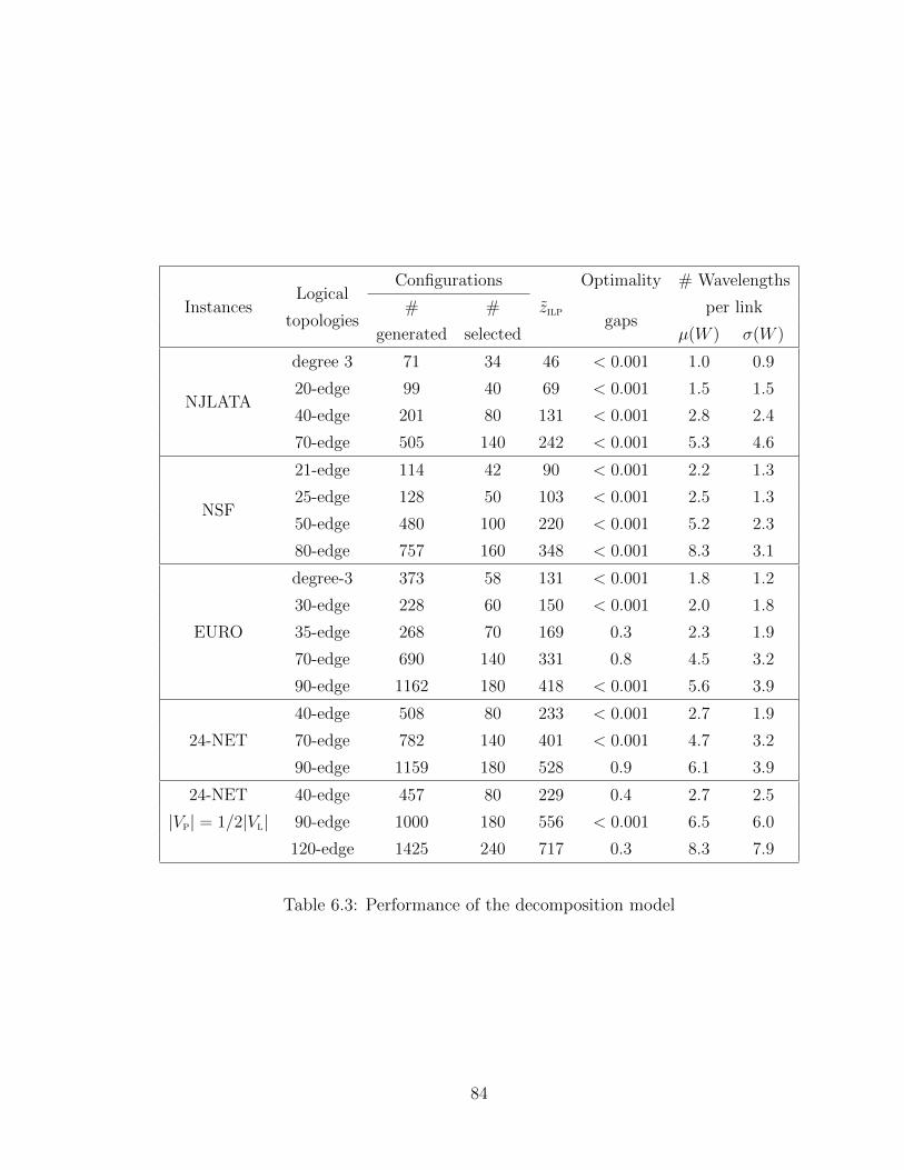
InstancesLogical
Configurations
zilp
Optimality # Wavelengths
topologies# #
gapsper link
generated selected µ(W ) σ(W )
NJLATA
degree 3 71 34 46 < 0.001 1.0 0.9
20-edge 99 40 69 < 0.001 1.5 1.5
40-edge 201 80 131 < 0.001 2.8 2.4
70-edge 505 140 242 < 0.001 5.3 4.6
NSF
21-edge 114 42 90 < 0.001 2.2 1.3
25-edge 128 50 103 < 0.001 2.5 1.3
50-edge 480 100 220 < 0.001 5.2 2.3
80-edge 757 160 348 < 0.001 8.3 3.1
EURO
degree-3 373 58 131 < 0.001 1.8 1.2
30-edge 228 60 150 < 0.001 2.0 1.8
35-edge 268 70 169 0.3 2.3 1.9
70-edge 690 140 331 0.8 4.5 3.2
90-edge 1162 180 418 < 0.001 5.6 3.9
24-NET
40-edge 508 80 233 < 0.001 2.7 1.9
70-edge 782 140 401 < 0.001 4.7 3.2
90-edge 1159 180 528 0.9 6.1 3.9
24-NET 40-edge 457 80 229 0.4 2.7 2.5
|Vp| = 1/2|Vl| 90-edge 1000 180 556 < 0.001 6.5 6.0
120-edge 1425 240 717 0.3 8.3 7.9
Table 6.3: Performance of the decomposition model
84

InstancesLogical # Non survivable Bandwidth
Topologies logical links Routing Protection
% # failure sets To be added (%) To be added (%) Redundancy ratio
NJLATAdegree-3 0.0 0.0 0.0 89.5 1.8
20-edge 10.0 2.5 1.0 133.3 2.0
Vp = Vl 40-edge 0.0 0.0 1.3 353.2 4.4
70-edge 0.0 0.0 3.0 777.0 8.8
NSF21-edge 14.3 1.7 0.0 153.5 2.1
25-edge 12.0 1.0 0.0 187.2 2.5
Vp = Vl 50-edge 0.0 0.0 2.1 249.6 2.8
80-edge 0.0 0.0 1.9 421.4 4.6
EUROdegree-3 31.0 1.1 0.6 168.6 2.2
30-edge 48.3 1.4 0.0 149.2 2.2
Vp = Vl 35-edge 28.6 1.4 0.0 239.0 3.2
70-edge 20.7 1.1 1.3 510.8 5.9
90-edge 14.4 1.0 2.2 612.3 6.8
24-NET 40-edge 32.5 1.8 0.7 258.4 3.3
Vp = Vl 70-edge 0.0 0.0 2.0 527.4 6.0
90-edge 0.0 0.0 3.2 564.7 6.2
24-NET 40-edge 10.0 1.2 0.4 316.3 3.8
|Vp| = 1/2|Vl| 90-edge 0.0 0.0 6.5 822.8 8.5
120-edge 0.0 0.0 7.8 1115.1 11.2
Table 6.4: Existence and dimensioning of a survivable logical topology (single-link
failures)
85

6.2.3 Quality of solutions
We now discuss the performance of the column generation model proposed in Section
6.1 in the context of 100% against single link failures, i.e., when F = {Fe = {e}, e ∈E} where E is the set of protection edges in the physical network (edges are undirected
links between two nodes). Results that are reported in Table 6.3 come from a set of
randomly generated virtual topologies with some degree k regular undirected graphs
and some m-edge general undirected graphs.
The number of generated configurations as well as the number of selected configu-
rations in the integer solutions are given in the third and fourth column, respectively.
Those numbers clearly show that a very small number of configurations out of the
overall number of potential configurations is needed in order to reach the optimal
solution of the linear relaxation of the master problem on the one hand, and a nearly
optimal integer solution on the other hand. The next three columns contain the
characteristics of the ILP solutions:
(i) optimal value z?lp of the linear relaxation of the master problem, (ii) integer
value zilp of the optimization model, and (iii) optimality gap.
We can observe that all optimality gaps are less than 2 percent, some even less
than 0.001, meaning that the integer solutions are nearly optimal ones. The last two
columns provide the mean (µ) and the variance (σ) of numbers of reserved wavelengths
on a physical link.
Comparing with the transport capacity values selected by [Todimala and Rama-
murthy, 2007], 6 wavelengths for njlata and 8 for nsf (values are not available for
euro and 24-net), we can conclude that it is more than enough. Indeed, the av-
erage wavelength requirements (± the corresponding variance) on the physical links
are 1.0 ± 0.9 (degree-3 logical network) and 1.5 ± 1.5 (20-edge logical network) for
njlata, 2.1 ± 1.3 (21-edge logical network) and 2.5 ± 1.3 (25-edge logical network)
for nsf with variance values such that the 6 and 8 threshold values are unlikely to be
exceeded.
In conclusion, the proposed solution process is very efficient, as practical optimal
solutions are obtained very often (solution with a gap smaller than 0.1% can be
considered optimal ones for practical purposes), which allow the proper identification
of the existence of a survivable logical topology.
86

6.2.4 Networking performances
The first set of experiments (Table 6.4) is again with single link failures only. In
Table 6.4, we report:
(i) the percentage of logical links which cannot survive the link failure of at least one
failure set,
(ii) for the logical links of (i), the average number of failure sets they cannot survive,
(iii) the additional bandwidth (% with respect to the initial transport capacities)
which is required in order to be able to map all logical links,
(iv) the additional bandwidth (% with respect to the adjusted transport capacities
after the routing/mapping of all logical links onto the physical links) which need to
be added in order to completely support IP restoration,
(v) the redundancy ratio assuming enough spare capacity is provided in order to allow
a successful IP restoration for all (physical) link failures.
In Table 6.4, we notice that redundancy ratio increases rapidly with number of
physical edges. That ratio is very high when number of physical edges becomes
significant, for e.g., is 6.8 in case of EURO network with 90 edges. The reason for
such a high ratio comes from the fact that: we maximize number of protected logical
links, not dimensioning protection capacity. See Fig. 6.2 where solid lines are logical
links while dash lines are their routed physical lightpaths. Label of each physical
lightpath consists of its name and its length covered by a parenthesis. Suppose that
logical link v1 → v3 fails, there are two options to restore that logical link: we route
the traffic either on logical path v1 → v2 → v3 or on v1 → v4 → v5 → v3. As our
model maximizes only number of protected links, thus, the two choices are the same.
If logical path v1 → v2 → v3 is selected, then the spare capacity is 10. Otherwise, if
the alternative path is used, the spare capacity is just 3, i.e., three times smaller than
in the case of the precedent path which is the shorter one in logical layer. So, as we
see, not dimensioning could waste a meaningful amount of capacity, hence leads to
significantly large redundancy ratios.
Comparing our results with those of [Todimala and Ramamurthy, 2007], we need
to be cautious as our randomly logical topologies are arbitrary ones (no special struc-
tures), those generated by [Todimala and Ramamurthy, 2007] have the planar cycle
property.
In the next set of experiments, we look at multiple failure scenarios (1-5) as
87

L3 (1)L5 (1)
V1V1
V2V2
V3V3
V5V5V4V4
L1 (5
)L2 (5)
L4 (1)
Fig. 6.2: Explain why redundancy ratio is a significantly large number.
described in Table 6.5. We conducted the experiments on several topologies and
reported the result in Table 6.6.
Scenarios Comments
1 only single link failure sets
2 single sets + 7% dual sets
3 single sets + 7% dual sets + 7% triple sets
4 single sets + 10% dual sets + 10% triple sets
5 single sets + 10% dual sets + 10% triple sets + 5% quadruple sets
Table 6.5: Multiple failure set scenarios
88

InstancesLogical Failure # Non survivable Bandwidth
Topologies Scenarios logical links Routing Protection
% # failure sets To be added (%) To be added (%) Redundancy ratio
NJLATA 20 edge
2 10.0 3.2 1.0 171.9 2.5
3 50.0 1.9 1.0 214.6 3.1
4 57.5 2.0 1.0 225.0 3.3
5 57.5 2.7 1.0 209.4 3.1
NJLATA 70 edge
2 0.0 0.0 3.0 862.8 9.7
3 8.6 1.0 3.0 908.9 10.3
4 8.6 1.0 3.0 917.5 10.4
5 8.6 1.0 3.0 987.4 11.1
EURO 90 edge
2 14.4 1.5 2.2 584.4 6.5
3 14.4 3.2 2.2 570.8 6.3
4 17.8 4.4 2.2 605.3 6.7
5 17.8 4.4 2.2 664.6 7.3
24-NET 90 edge
2 2.8 1.0 3.2 591.9 6.5
3 2.8 1.0 3.2 526.5 5.8
4 2.8 1.0 3.2 453.1 5.0
5 2.8 1.0 3.2 450.3 5.0
24-NET 120 edge
2 18.3 1.1 7.8 1097.5 11.1
3 18.3 1.1 7.8 1187.6 11.9
|Vp| = 1/2|Vl| 4 18.8 1.1 7.8 1153.0 11.6
5 17.5 1.2 7.8 1287.3 12.9
Table 6.6: Existence and dimensioning of a survivable logical topology (multiple-link
failures & |Vp| = 1/2|Vl|)
6.3 Conclusion
We proposed a first scalable ILP model for the design of survivable logical topologies,
which allow the exact solution of most of the data instances considered so far in
the literature. In addition, not only the proposed model allows checking whether a
survivable logical topology exists or not, but, when none exists, it still constructs
the largest possible survivable logical topology, with indication on an appropriate
dimensioning of the physical links.
In this work, we do not dimension protection capacity, only maximize the amount
of protected links, thus it results in a very high redundancy ratio. That means a
significant amount of protection capacity can be waste if network dimensioning does
not be taken into account. A possible extension of this work is to combine protected
capacity with protection one.
89

In future work, we will investigate how to improve the solution of the proposed
model with heuristics in order to solve larger data instances (including data instances
with multi-unit logical links), closer to the ones encountered in the current IP-over-
WDM networks. We believe that there is a lot of room for improving the current
solution scheme and for combining it with heuristics in order to speed it up.
Another direction for this study is to consider node failure in the physical layer.
To deal with physical node failures, we simulate a failing node by the failure of the
links that are adjacent to that node.
90

Chapter 7
Design of a multirate optical
network architecture
New high capacity optical devices such as 40Gbps and 100Gbps regenerators are pow-
erful tools to deal with the continuous traffic growth. However, economic incentives
make network operators deploy those new devices with minimum capital investment.
As completely upgrading the current backbone network with new devices is impossi-
ble due to their expensive price, a cost-effective dimensioning plan where equipment
of heterogeneous optical rates co-exist in a network (mixed line rate WDM networks)
is necessary.
When it comes to regenerators, besides transmission reach and capacity, max-
imum number of hops (because of physical impairment) and maximum number of
sites where regenerators can be deployed have to be taken into account. Additionally,
limitation on wavelength capacity per fiber and per node must be considered accord-
ing to reality. The design problem becomes even more complicated when grooming
criteria is included, hence it is quite difficult to develop a general solution.
By applying a decomposition methodology with a novel formulation of hierarchical
pricing sub-problems, an exact and scalable algorithm is proposed in our work. Since
no ad-hoc requirements are needed in our solution, new physical criteria can be easily
included thanks to the generality of our formulation.
Numerical results in Section 7.5 show that, firstly, the percentage distribution of
transceivers grouped by MTD is stable while the traffic volume grows. Secondly, we
see that 10Gbps transceivers takes the major part in the optimal solution in contrast
91

to the minor part of 100Gbps and 40Gbps. But such a difference is reduced with
the evolution of traffic. Moreover, number of 100 Gbps transceivers grows faster
than the one of 40Gbps transceiver. Thirdly, we witness a huge impact of maximum
regenerable site constraint on the transceiver cost. The main idea of restricting the
maximum number of regenerable sites is to gather regenerators to few sites in order to
take advantage of sharing support devices, such as cooling systems. By that way, we
can reduce the operating cost (OPEX). In return, we have pay more CAPEX. Thus,
our result helps network designer to make a trade-off between OPEX and CAPEX
when planing such a system.
Section 7.1 introduces the problem that this research addresses. Cost information
of optical equipment is given in Section 7.2. We propose our decomposition model in
Section 7.3. The flexibility of our model shows in Section 7.3.5 where we can easily
adapt it to undirected network. Since our solution process has minor differences to
the general multi-pricing decomposition algorithm that Section 2.4.2 describes, we
explain in detail our computational approach in Section 7.4. Section 7.5 reports the
numerical result that we got. Conclusions are draw in Section 7.6.
7.1 Problem description
Next three paragraphs present the network architecture, the assumption constraints,
and the cost objective, respectively.
Network architecture
The study considers backbone networks with the following architecture.
Node structure in our backbone network is an OXC that supports three basic
operations. First, it can let a lightpath pass through without being regenerated by
using an optical bypass. Second, a lightpath can be regenerated in order to improve
its optical quality that is degraded during the transmission. Third, it can add or drop
a wavelength that means finishing a single-hop lightpath or starting a new one from
the electrical layer.
We work with multiple rate networks, meaning that an optical link contains dif-
ferent wavelengths at different bit-rates.
A lightpath, also called single-hop lightpath, is an optical path without any regen-
eration, otherwise it is called multi-hop lightpath. Actually, a multi-hop lightpath is
92

a sequence of several single-hop lightpaths. Moreover, a single-hop lightpath operates
at only one bit-rate.
Actually, we do no consider grooming capacity in our model as it is performed
in the electrical layer. Node cost in our model consists of transceivers costs and
regenerator costs. We assume that regenerators are deployed only at nodes. On
other words, there is no in-line regenerator. Network cost is simply the sum of all
node costs.
Node equipment is a function of bit-rate capacity and maximum distance reach
which is defined as the maximal possible length of a single-hop lightpath. Certainly,
there is a limitation to the length of a multi-hop lightpath, but this can be easily
approximated by setting a constraint on the number of regenerators. Information
about those costs are given in Table 7.1.
Fig. 7.1 shows a simple multirate network. Let TRBD be the cost of transceiver
TX + RX of bandwidth B and maximum distance reach D. Those parameters are
defined in Table 7.1. The total network cost consists of the transceiver cost between
A and B (2×TR401000 +2×TR100
1000), the transceiver cost between B and C (2×TR40750 +
2× TR100750) and the one between A and C (2× TR10
1750). Then, the whole transceiver
cost of the example in Fig. 7.1 is
2× TR401000 + 2× TR40
750 + 2× TR100750 + 2× TR100
1000 + 2× TR101750.
Line cost (such as amplifiers) is not considered here because it is not impacted by
optimization process.
Assumptions
In order to avoid the expensive cost of wavelength converters, we consider wavelength
continuity assumption in the sense that in a single hop lightpath, a same wavelength
is used for every link. We also assume that there is a limited number of available
wavelengths in a link.
In our model, one important constraint is applied: we limit the number of nodes
where regenerators are deployed. The rationale comes from the fact that, in prac-
tice, regenerators are gathered in few nodes for being effectively managed as well as
minimizing the overall cost of supporting equipment such as cooling systems.
We also take into account a constraint that implies a limit on the number of hops
93

Fig. 7.1: A simple multirate optical network
of a multi-hop lightpaths. This constraint is applied to prevent the delay between
optical channels from being too large.
Objective
With a given network topology, traffic demands, and cost distribution of different
kinds of transceivers and regenerators, we design a network that satisfies all demands
at minimum transceiver cost while satisfying the previously described constraints.
7.2 Cost model
In this section, we propose a model that evaluates the transceiver cost of a network.
Our numbers are taken from [Huelsermann et al., 2008]. However, [Huelsermann et al.,
2008] does not contain informations about 40 Gbps transceivers and regenerators at
3000 km - MTD (Maximum Transmission Distance), nor any information about 100
Gbps transceivers and regenerators. One way to get an idea about missing information
is to use the cost formulation given in [Simmons, 2005] to calculate the transceiver
costs and use back-to-back (B2B) regenerators whose prices are two times the cost
of a transceiver. The amplifier costs are exactly the same as in [Huelsermann et al.,
2008]. We were surprised that, in [Huelsermann et al., 2008], the dispersion cost
depends on MTD and bit-rate, thus, we decided to assume the dispersion cost is 0.01
94

(thousand dollars) which is the average of the values given in [Huelsermann et al.,
2008].
We decided to build the traffic of a network topology such that its bandwidth
demand between two cities are in proportion of their populations. We use the for-
mulation (27-29) given in [Batayneh et al., 2011a] to produce such a traffic. The
population of a city is easily found in Internet [Brinkhoff, 2014].
In Table 7.1, cost unit is a thousand dollars.
Transceiver Regenerator Amplifier Dispersion
costtrmtd(p),r costreg
mtd(p),r costapmtd(p),r costds
mtd(p),r
References [Simmons, 2005] (*) [Huelsermann et al., 2008] (**) ** B2B ** **
mtd (km) r = 10 Gbs
750 lh 1 1 1.4 2 1.92 0.01
1,500 elh 1.25 1.25 1.75 2.5 2.77 0.01
3,000 ulh 1.56 1.67 2.34 3.12 3.45 0.01
mtd (km) r = 40 Gbs
750 3 3.75 5.25 6 1.92 0.01
1,500 3.75 5.17 7.24 7.5 2.77 0.01
3,000 4.68 9.36 3.45 0.01
mtd (km) r = 100 Gbs
750 5 10 1.92 0.01
1,500 6.25 12.5 2.77 0.01
3,000 7.8 15.6 3.45 0.01
Table 7.1: Cost model (MTD = Maximum Transmission Distance).
7.3 Decomposition model
We formulate a column generation model with two pricing problems. One pricing
problem generates wavelength configurations while the other generates a multi-hop
path configurations. We introduce our definitions and notations in Section 7.3.1.
Then, the master (Section 7.3.2) and the two pricing problems (Section 7.3.3 and
95

7.3.4) are detailed. Section 7.3.5 explains how to adapt the decomposition model to
undirected networks.
7.3.1 Definitions and notations
We explain our notations and variables in this section. Definition of wavelength
configuration and of multi-hop path configuration are given in the next paragraphs.
Such configurations are generated by the two pricing problems that we introduce in
the sequel.
So let:
• s : source.
• d : destination.
• Drsd: number of demand units between vs and vd, with rate r.
• SD = {{vs, vd} : Drsd > 0 for at least one r ∈ R}
• r : granularity/rate (10 Gbps, 40 Gbps, 100 Gbps).
• nreg: maximum number of nodes where regeneration can occur
Also, we have:
• G = (V, L) where
– V is the set of nodes (generic index v), and
– L is the set of (directed) links (generic index `)
• W : maximum number of available wavelengths.
• regv : maximum number of regenerator ports at node v.
Variables of our model are as follows.
• zγ : number of times configuration γ is selected.
• nrij : number of lightpaths with bit-rate r between vi and vj, which belong to
the set of selected wavelength configurations.
• yπ : number of selected copies of multi-hop path configuration π.
• xv : 1 if node v is used for regeneration, 0 otherwise.
96

Wavelength configurations
The optimization model relies on a set of potential wavelength configurations, which
are defined as follows.
A wavelength configuration γ is a set of disjoint single-hop lightpaths, all routed
on the same wavelength.
• Γ: set of configurations (generic index γ)
• costγ: cost of configuration γ (defined in equation (7.1))
• P set of lightpaths with
– P =⋃
(vi,vj)∈V×VPij
– Pij: set of (single-hop) lightpaths from vi to vj (generic element p)
– characteristic vector: δ`p = 1 if ` belongs to p, 0 otherwise.
• Characteristic vector of a wavelength configuration γ ∈ Γ: for p ∈ P
aγpr =
1 if wavelength configuration γ contains
lightpath p ∈ P with bit-rate r
0 otherwise.
Multi-hop path configurations
A multi-hop path configuration, denoted by π is a wavelength route defined as a se-
quence of lightpaths, where all the lightpaths have the same bit-rate. Notice that the
lightpaths belonging to a given multi-hop path configuration can be associated with
different wavelengths. Let Π denote the set of all possible multi-hop path configura-
tions with
Π =⋃
(vs,vd)∈V×V
⋃r∈R
Πrsd,
where Πrsd is the set of multi-hop path configurations between vs and vd and bit rate
r.
Characteristic vectors of a multi-hop path configuration π ∈ Πrsd: for (vi, vj) ∈
97

V × V
bπij =
1 if multi-hop path configuration π contains
a lightpath with bit-rate r from vi to vj,
0 otherwise
eπv =
1 if v is a regeneration node of π
0 otherwise
7.3.2 Master model
The objective of the optimization model is to minimize the network cost, as estimated
by the regenerator costs, as well as the transceiver/receiver, amplifier and dispersion
equipment costs. The model is expressed as follows.
min∑γ∈Γ
costγzγ
where
costγ =∑p∈P
∑r∈R
costregmtd(p),r a
γpr (7.1)
with costregmtd(p),r being the regenerator cost of path p with rate r. Values can be
found in Table 7.1 for various parameters. The master problem is subject to following
constraint:
Limited number of available wavelengths∑γ∈Γ
zγ ≤ W (7.2)
Computation of the number of lightpaths with bit-rate r from vi and vj
nrij =∑γ∈Γ
∑p∈Pij
aγpr zγ r ∈ R, (vi, vj) ∈ V × V (7.3)
Bandwidth demands∑π∈Πr
sd
yπ = Drsd r ∈ R, (vs, vd) ∈ SD (7.4)
98

Do not use more than the number of available lightpaths belonging to the selected
multi-hop path π configurations
∑π∈Πr
bπij yπ ≤ nrij r ∈ R, (vi, vj) ∈ V × V (7.5)
Limit on the number of regenerator ports at node v
∑π∈Π
eπv yπ ≤ xvregv v ∈ V (7.6)
Limit on the number of nodes with regeneration equipment
∑v∈V
xv ≤ nreg. (7.7)
7.3.3 Pricing I: generation of wavelength configurations (γ)
The first pricing problem is to generate wavelength configurations and is defined as
follows.
input: Dual values of constraints (7.2) ( u0), (7.3) ( u1ijr), and set of pre-
enumerated single-hop lightpaths.
output: An improving configuration γ ∈ Γ described by its characteristic vector
(aγpr)p∈P,r∈R.
The formal formulation is expressed as:
min costγ = costγ − u0 −∑r∈R
∑(vi,vj)∈V×V
∑p∈Pij
u1ijrapr
subject to:
Link disjointness requirement
∑r∈R
∑p∈P
δ`p apr ≤ 1 ` ∈ L (7.8)
99

Reach vs. rate
aprr ≤ rlh p ∈ P : len(p) ≥ plh (7.9)
aprr ≤ relh p ∈ P : len(p) ≥ pelh (7.10)
aprr ≤ rulh p ∈ P : len(p) ≥ pulh (7.11)
Domain of the variables
apr ∈ {0, 1} p ∈ P, r ∈ R. (7.12)
7.3.4 Pricing II: generation of multi-hop path configuration
(π)
The second pricing problem is to generate mutli-hop path configurations and is defined
as follows.
input: Dual values of constraints (7.4) ( u2ksdr), (7.5) ( u3k
ijr) (7.6) ( u4kv ) ; bit
rate r ; pair of source and destination nodes {vs, vd}output: An improving configuration π ∈ Πr
sd described by its characteristic vector
(bπij)vi,vj∈V×V and eπv .
The formal formulation is expressed as:
min costπ = −u2ksdr −
∑ij
biju3kijr −
∑v
u4kv ev
subject to:
1. Flow Conservation∑(vi,vj)∈w+(v)
bij =∑
(vi,vj)∈w−(v)
bij = ev (v 6= s, d) (7.13)
2. In/Out Source Destination Flow∑(vi,vj)∈w+(s)
bij =∑
(vi,vj)∈w−(d)
bij = 1 (7.14)
100

7.3.5 Adaptation to undirected model
The presented model can be easily converted to undirected one by using undirected
topology, undirected path, and undirected link instead of directed ones. In that case,
Master as well as Wavelength Configuration Pricing keep being the same as in the
directed case. We only need to replace Eq. (7.13) and (7.14) by new undirected
versions for Multi-hop Path Configuration Pricing as follows.
1. Flow Conservation ∑(vi,vj)∈w(v)
bij = 2ev (v 6= s, d) (7.15)
2. In/Out Source Destination Flow∑(vi,vj)∈w(s)
bij =∑
(vi,vj)∈w(d)
bij = 1 (7.16)
7.4 Solution of the models
The outline of the solution process is depicted in the flow chart Fig. 7.2. We start with
a restricted master problem (RMP) which is made of an artificial solution consisting
of several dummy columns. The objection of such an solution is far from the optimal
one that we have to obtain through a repeat process.
Step 1 The RMP is optimally solved to get the corresponding dual values which are
the input parameters of the first pricing problem (wavelength pricing problem).
Step 2 Searching for the solution of the wavelength pricing problem whose reduced
cost is negative. If such a solution is found then it will be added back to the
RMP since the pricing solution is the augmented column to the RMP and Step
1 is repeated. Otherwise, we continue to Step 3.
Step 3 The second pricing problem (multi-hop pricing problem) is solved with a
same set of dual values in Step 2 in order to find a solution with negative
reduced cost. If such a solution exists, it is added back to the RMP and the
process is repeated from Step 1. Otherwise, we jump to Step 4
101

Step 4 Solve the RMP with all integer constraints to get the final ILP solutions since
we know that the relax incumbent solution after Step 3 is the optimal RMP
solution.
Each step is either an integer programming problem (Step 2,3,4) or a linear pro-
gramming problem (Step 1). Those problems are implemented in OPL, an optimiza-
tion programming language, and are solved by using software IBM ILOG CPLEX
Optimization Studio 12.5.
ε-optimalILP solution
Fig. 7.2: Outline of the solution process
7.5 Numerical experiments
Our plan of experiments consists of two parts. The first part is to solve the problem
for different traffic volumes in order to acknowledge the importance of high capacity
transceivers (100 Gbps transceivers) in reducing CAPEX of WDM networks. The
second part is to investigate the impact of maximum available regenerable sites. We
would like to discover the relationship between that constraint with the network
cost so that network designers can have some ideas when taking into account such a
constraint.
Section 7.5.1 introduces how we prepare network traffic between cities in order to
reflect the real life situation. Section 7.5.2 describes our analysis about the impact of
102

traffic and of maximum regenerable site constraint in detail.
7.5.1 Data instances
We conducted experiments on the US-24 network with 24 nodes and 84 directed
links (see Fig. 7.4) [Batayneh et al., 2011a]. We use the same traffic generation as
in [Batayneh et al., 2011a]. Traffic is generated on every node pair where each node
corresponds to a city, and the traffic is a function of the population in the cities
associated with the endpoints. Bandwidth demand on a node pair corresponds to the
product of population of the two end nodes. Actually, such a demand of a node pair
is calculated as follows.
co coefficient for generating traffic.
popi population in city i
totpop total population =∑i
popi
demandij traffic demand from city i to city j
Traffic demand from city i to city j is computed as follows.
demandij = co×popi × popj
totpop× totpop× popi
popi + popj(Gbps). (7.17)
We then derive granularity bandwidth demands (grooming) from demandij by the
following simple scheme.
D100sd =
⌊demandsd
100
⌋D40sd =
⌊demandsd − 100×D100
sd
40
⌋D10sd =
⌈demandsd − 100×D100
sd − 40×D40sd
10
⌉where co (Eq. 7.17) represents the traffic volume. In our experiments (as in [Batayneh
et al., 2011a]), co varies from 2,048 up to 20,480 in order to simulate traffic volume
patterns at different peek intervals. Hereby, we define traffic load over the network
as the sum of all traffic demands between node pairs:
103

traffic load =∑ij
demandij.
Traffic load represents the traffic volume that takes place in network. Table 7.2
shows the correspondence between co and traffic load.
co 2,048 4,096 6,144 8,192 10,240 12,288 14,336 16,384 18,432 20,480 22,528 24,576
traffic load (Gbps) 957 1,915 2,873 3,830 4,787 5,745 6,703 7,660 8,617 9,575 10,533 11,490
Table 7.2: Traffic load vs. co
Fig. 7.3 shows the traffic demand distributions per node pair with respect to
different traffic load. Such a distribution is formed by sorting the node pair traffic
demands in descending order of their demand. In Fig. 7.3, X-axis indicates node pair
index (ranked by traffic demand) which spreads from 1 to 552 while Y-axis presents
the corresponding demand. It turns out that, firstly, the form of our traffic patterns
remains the same with our traffic generated model, and secondly, 36% of node pairs
contributes 76% of network traffic while 18% of node pairs occupies 56% of network
traffic.
104

Fig. 7.3: Traffic demand distribution
105

Fig. 7.4: US-24 network
106

7.5.2 Impact of traffic volume and physical constraints on
CAPEX
Percentage pattern of transceivers grouped by MTD
Fig. 7.5 reports the evolution of the average percentage of transceivers by 750km,
1,500km and 3,000km against traffic load. For each traffic load, such an average is
defined as follows:
AVG(percentage) =percentage12 + percentage18 + percentage24
3
where percentagex is the percentage of a kind of transceiver (750km, 1500km or
3000km) in the quasi-optimal solution of the problem whose amount of regenerable
sites is x. We did the linear regression (f(x) = a× x + b) on the set of average per-
centage for each kind of transceiver (classified by MTD) and displayed the obtained
a and b on the top right of Fig. 7.5.
0
20
40
60
80
100
957 1915 2872 3830 4787 5745 6702 7660 8617 9575 10533 11490
AV
G(p
erc
en
tage
)
Traffic load
transceiver of 3000kms (a=0.000,b=73.820)transceiver of 1500kms (a=0.000,b=22.855)
transceiver of 750kms (a=0.000,b=3.275)
Fig. 7.5: Average of transceiver percentages of 750km, 1500km and 3000km
107

MTD Mean Standard Deviation
3000km [71.4-75.6] [0.7-2.0]
1500km [21.4-24.9] [0.3-2.0]
750km [02.8-04.8] [0.3-1.0]
Table 7.3: Statistics of the percentage average
Table 7.3 shows the mean and the standard deviation of the set of AVG(percentage)
with different traffic load for each MTD.
It turns out that transceivers of 3000km takes the largest part in the quasi-optimal
solution (∼73%), then transceiver of 1500km takes about 23% and the ones of 750km
takes the smallest part (∼4%). This fact makes sense since it is obvious that using
long distance transceivers reduces the need of regenerators.
Fig. 7.5 shows that traffic evolution has no significant impact on the average
percentage distribution of the set of transceivers grouped by MTD since parameter a
keeps being 0 despite traffic increase.
Percentage pattern of transceivers grouped by bit-rate
Fig. 7.6 is similar to Fig. 7.5, except that its transceivers are classified by bit-rate
instead of MTD. We also fit the data with the linear regression (f(x) = a× x+ b).
This figure shows clearly that transceivers of 10Gbps has the largest percent-
age (>50%) while other kinds of transceivers (40Gbps and 100Gbps) takes the rest.
Moreover, transceiver percentage of 10Gbps slowly decreases with the evolution of
traffic load (a = −0.0015 < 0) while transceiver percentages of 40Gbps and 100Gbps
increase (a = 0.0010 and a = 0.0006).
The increasing momentum of transceivers of 100Gbps (a = 0.0010) is higher than
the one of transceivers of 40Gbps (a = 0.0006). It means, in comparison with the
percentage of transceivers of 40Gbps, the percentage of transceivers of 100Gbps is
increasing in accordance with traffic load increment. However, when the traffic load
is relatively small, both percentages have a meaningless difference.
108

0
20
40
60
80
100
957 1915 2872 3830 4787 5745 6702 7660 8617 9575 10533 11490
AV
G(p
erc
en
tage
)
Traffic load
transceiver of 10Gbps (a=-0.0015,b=86.324)transceiver of 100Gbps (a=0.0010,b=5.711)
transceiver of 40Gbps (a=0.0006,b=7.857)
Fig. 7.6: Average of transceiver percentages of 10Gbps, 40Gbps and 100Gbps
109

Impact of constraint of maximum regenerable sites over transceiver dis-
tribution (grouped by bit-rate)
Fig. 7.7 compares two extreme cases where maximum amount of regenerable sites are
12 and 24. The former case is when such an amount is half number of nodes while the
latter case means that every node can be a regenerable site. In Fig. 7.7, the dash lines
are for the 12 regenerable sites case while the solid lines are for the 24 regenerable
sites case. Blue and red indicates transceiver of 10 Gbps and 100 Gbps, respectively.
Obviously, in the case of maximum 12 regenerable sites, the optimal solution uses
more transceivers of 100Gbps and less transceivers of 10Gbps than in the case of
maximum 24 regenerable sites. It makes sense since the first case has fewer choices of
node to deploy regenerators than the second case has. We conclude that when such a
constraint gets stricter, the optimal design has to deploy more and more transceivers
of high capacity (100Gbps).
Fig. 7.7 also confirms the trend of using less transceivers of 10Gbps and more
of 100Gbps as the traffic load increases. The next paragraph makes a quantitative
comparison about the impact of maximum regenerable sites on the deployment cost.
Since we do not consider grooming, the number of transceivers of a specific bit-rate
at the end nodes of working paths is constant; consequently we can pre-calculated
their numbers. However, the number of transceivers that are deployed at intermediate
nodes depends on the maximum number of regeneration sites.
Impact of constraint of maximum regenerable sites over the deployment
cost (CAPEX)
The main idea of restricting the maximum number of regenerable sites is to gather
regenerators to few sites in order to take advantage of sharing support devices, such as
cooling systems. By that way, we can reduce the operating cost (OPEX). As shown in
previous paragraphs, such a constraint results in requiring more 100Gbps and 40Gbps
transceivers, in the other words, increasing the deployment cost (CAPEX).
Fig. 7.8 shows the dependency of the transceiver costs on the maximum available
regenerable sites. E.g., the transceiver cost in the case of 24 regenerable sites over
the one of 12 regenerable sites may vary from 21.4% to 50.3%.
110

0
20
40
60
80
100
957 1915 2872 3830 4787 5745 6702 7660 8617 9575 10533 11490
Pe
rce
nta
ge
Traffic load
Transceivers 10Gbps (12)Transceivers 100Gbps (12)
Transceivers 10Gbps (24)Transceivers 100Gbps (24)
Fig. 7.7: Comparison of percentages of transceivers grouped by bit-rate that is made
between the case of maximum 12 regenerable sites and of maximum 24 regenerable
sites
111

5000
6000
7000
8000
9000
10000
11000
12000
13000
957 1915 2872 3830 4787 5745 6702 7660 8617 9575 10533 11490
Co
st
Traffic load
ngen=12ngen=18ngen=24
Fig. 7.8: Cost comparison between different amount of maximum regenerable sites
112

7.6 Conclusion
We develop a decomposition method to solve the multi-rate design problem taking
into account the constraint of maximum regenerable sites which, to the best of our
knowledge, has not been considered in literature. We discover that the traffic evolu-
tion has almost no impact on the percentage distribution of transceiver grouped by
MTD. When we group transceivers by bit-rate, when the traffic grows we see the per-
centage of 100Gbps transceivers increases fastest, then the one of 40Gbps transceiver,
as opposed to the reduction of the percentage of 10Gbps. Those points could be hints
to develop a high scalable heuristic for huge networks where such an extract method
is intractable.
We study the restriction on maximum regenerable sites and see a huge impact on
the deployment cost. For US-24 network, when reducing the number of regenerable
sites from 24 to 12, we can see that the increase in deployment cost is between 21.4%
and 50.3%. Based on such information, a network designer can make a appropriate
compromise between OPEX and CAPEX.
7.7 Future work
Our proposed models are for a network with a general pattern of traffic. In this
section, we assume that we are given different traffic matrices, where each traffic
matrix corresponds to the traffic over a given time period within the time horizon
under study. The goal is then to find a network design that allows the provisioning
of the traffic for all time periods, at minimum cost. We next explain how to modify
the model presented in the previous section. We re-use the same notations and
variables, except for few exceptions, which are next described. In future, we will do
the experiments with networks that have multiple traffic matrices.
NotationsT Set of time periods within the time
horizon (generic index t)
Drtsd Number of demand units from vs to vd,
with rate r during time period t.
113

Variables yπ are replaced by:
ytπ number of selected copies of multi-hop
path configuration π during period t.
The objective function remains unchanged while constraints (7.4), (7.5) and (7.6)
are modified as follows:∑π∈Πr
sd
ytπ = Drtsd r ∈ R, vs, vd ∈ SD, t ∈ T (7.4’)
Do not use more lightpaths that the number of available lightpaths belonging to the
selected multi-hop path configurations
∑π∈Πr
bπij ytπ ≤ nrij r ∈ R, (vi, vj) ∈ V × V, t ∈ T (7.5’)
Restriction on the number of regenerator ports at node v
∑π∈Π
eπv ytπ ≤ xvregv v ∈ V, t ∈ T (7.6’)
It is possible, but not straightforward, to apply our proposed formulation to elastic
optical networks. As indicated in [Gerstel et al., 2012], two important properties of
elastic optical networks are: firstly, the optical spectrum can be divided up flexibly
and secondly, the transceivers can generate elastic optical paths (EOPs); that is, paths
with variable bit rates. The first property implies that we do not have a fixed number
of wavelengths and bit-rate per wavelength is variable. In order to implement those
conditions, we can remove the constraint on the maximum number of wavelengths and
the integer granularity on wavelength bit-rate. We denote, in that case, wavelength
bit-rates by a set of float variables. The second property means that we have to
take into account grooming in our formulation. So, even it is possible to extend our
proposed model to elastic optical networks, it need to invest serious effort.
114

Chapter 8
Conclusion and future works
8.1 Conclusion
Scalability and quality estimation are two important aspects of a network design
solution. Achieving both of those characteristics are difficult for heuristics. Decom-
position techniques allow to obtain such criteria if we have a proper mathematical
decomposition.
This thesis developed several innovative decomposition models for various network
design problem and, consequently, get very good results in terms of performance and
solution quality for some basic optimization planning problems arising in the design
of optical networks. This work explores four principal aspects.
Firstly, with help of large-scale decomposition model, the impact of wavelength
continuity assumption on the ε-optimal solutions of p-cycle and FIPP network designs
is investigated. Our numerical results shows that, when it comes to p-cycle and FIPP
designs, a fair amount of money can be saved by implying wavelength continuity
constraint. Such a constraint simplifies the network design complexity as well, thus
allows us to explore larger instances than previous studies and, at the same time,
combine working and protection capacities in an objective.
Secondly, a scalable multi-pricing column generation algorithms is proposed for
FDPP p-cycles subject to multiple link failures that delivers ε-optimal solutions. Such
a algorithm reconfirms that FDPP design has a better redundancy ratio over FIPP
designs. Moreover, we formally show that, by using our proposed framework, node
failure is just a special case of multiple link failure.
115

Thirdly, a network-flow based column generation is also successfully applied to
the survivability logical topology design problem. Thanks to the network flow for-
mulation, such a problem is solved at a large scale and subject to multiple link
failures that can not be obtained with other existed studies which follows the cut-set
based approach. The flexibility of that network-flow based CG algorithm allows us
to explorer several options to a survivability logical mapping, for e.g., what is an
optimal amount of spare capacity should be added in order to guarantee a successful
restoration against a certain network failure. Since we do not optimize the protection
capacity, we got very high redundancy ratios. That means a meaningful amount of
protection capacity may be wasted.
Fourthly, we attacked multirate cross-layer design problem by introducing a multi-
ple pricing CG algorithm that helps us to investigate on the impact of various physical
constraints, for e.g., number of available regenerator sites, maximum number of slots
in optical switches, etc. By formulating the optical layer and the physical layer into
two separate pricing problems, a great flexibility of introducing physical and optical
constraints is obtained since the inter-dependent between those layers are moved into
the master problem. When studying the restriction on maximum regenerable sites, we
see a huge impact of such a constraint on the deployment cost. Our proposed model
gave an exact value on the deployment cost according to each constraint setting.
Based on such information, a network designer can make a appropriate compromise
between OPEX and CAPEX.
The thesis is a successful story of applying large-scale decomposition methodology
to telecommunication network design. It shows that, when dealing with current
industrial optical networks, scalability, solution quality as well as model flexibility
are very possibly archived with CG methodology if we can come up with an effective
decomposition.
8.2 Future works
The work in this thesis can be extended in three directions.
Firstly, our proposed decomposition models solve larger instances than the ones
that have been studied in the literature. We also consider complicated constraints,
for e.g., multiple link/node failures, that are often ignored in many studies. In our
116

thesis, we solve up to 24-nodes networks. Such a limitation is set by the current
computational power that is available to us. In order to improve the scalability,
several heuristics, such as warm start, parallel computing, lazy constraints, and ad-
hoc speciality algorithms (shortest path, network flow, bender decomposition..) can
be applied to both master and price problems. Those techniques will improve the
solution process in order to meet the computational challenging coming from future
hypothetical large-scale optical networks, i.e, CORONET Global Network (see [Chiu
et al., 2009]) which is an hypothetical optical network with 100 nodes and 136 links.
The next generation decomposition models should be able to solve such a large-scale
network within few hours.
Secondly, our decomposition algorithms are implemented by CPLEX OPL which
is a general purpose optimization language. In order to avoid re-invent CG implemen-
tation every time, an universal CG framework should be developed so that network
designer can focus more on the design rather than on implementation. An universal
CG framework should be implemented in C++ as well as in multi-threading platform
in order to gain as much performance as possible.
Thirdly, up to two network layers are considered in our thesis. Beyond two layer
designs are impossible for our current CG implementations due to the computing
limitation. In order to attack more than two layers in network design, we can focus
on developing heuristics that speed up the solving process of the pricing problem
and/or build a good initial set of columns in the master problem.
117

Bibliography
[Barnhart et al., 1998] Barnhart, C.; Johnson, E.L.; Nemhauser, G.L.; Savelsbergh,
M.W.P., and Vance, P.H. Branch-and-Price: Column Generation for Solving Huge
Integer Programs. Operations Research, 46(3):316–329, 1998.
[Batayneh et al., 2006] Batayneh, M.; Zhu, H.; Song, L., and Mukherjee, B. Cost-efficient
WDM mesh network design with line cards of multiple ports. In IEEE Global
Telecommunications Conference - GLOBECOM, pages 1 –5, 2006.
[Batayneh et al., 2008] Batayneh, M.; Schupke, D.A.; Hoffmann, M.; Kirstaedter, A., and
Mukherjee, B. Optical network design for a multiline-rate carrier-grade Ethernet
under transmission-range constraints. Journal of Lightwave Technology, 26:121–
130, January 2008.
[Batayneh et al., 2011a] Batayneh, M.; Schupke, D.A.; Hoffmann, M.; Kirstadter, A.,
and Mukherjee, B. On routing and transmission-range determination of multi-
bit-rate signals over mixed-line-rate WDM optical networks for carrier ethernet.
IEEE/ACM Transactions on Networking, 19(5):1304–1316, October 2011a.
[Batayneh et al., 2011b] Batayneh, M.; Schupke, D.A.; Hoffmann, M.; Kirstaedter, A.,
and Mukherjee, B. Reliable multi-bit-rate VPN provisioning for multipoint carrier-
grade ethernet services over mixed-line-rate WDM optical networks. IEEE/OSA
Journal of Optical Communications and Networking, 3(1):66–76, January 2011b.
[Brinkhoff, 2014] Brinkhoff, Thomas. Population statistics for countries, administrative
areas, cities and agglomerations. http://www.citypopulation.de/, 2014. (last
visited on 21 April 2014 ).
118

[Chiu et al., 2009] Chiu, A.L.; Choudhury, G.; Clapp, G.; Doverspike, R.; Gannett, J.W.;
Klincewicz, J.; Li, Guangzhi; Skoog, R.A.; Strand, J.; Von Lehmen, A., and Xu,
Dahai. Network design and architectures for highly dynamic next-generation ip-
over-optical long distance networks. Journal of Lightwave Technology, 27(12):1878–
1890, 2009.
[Choi et al., 2002] Choi, H.; Subramaniam, S., and Choi, H.A. On double-link failure
recovery in WDM optical networks. In IEEE Annual Joint Conference of the IEEE
Computer and Communications Societies - INFOCOM, volume 2, pages 808–816,
2002.
[Cholda and Jajszczyk, 2007] Cholda, P. and Jajszczyk, A. Reliability assessment of optical
p-cycles. IEEE/ACM Transactions on Networking, 15(6):1579–1592, December
2007.
[Cholda and Jajszczyk, 2010] Cholda, P. and Jajszczyk, A. Recovery and its quality in
multilayer networks. Journal of Lightwave Technology, 28(4):372–389, 2010.
[Chu et al., 2003] Chu, X.; Li, B., and Chlamtac, I. Wavelength converter placement under
different RWA algorithms in wavelength-routed all-optical networks. IEEE Trans-
actions on Communications, 51(4):607 – 617, April 2003.
[Chvatal, 1983] Chvatal, V. Linear Programming. Freeman, 1983.
[Cisco, 2013] Cisco, . Cisco Visual Networking Index: Forecast and Methodol-
ogy, 2012-2017. http://www.cisco.com/c/en/us/solutions/collateral/
service-provider/ip-ngn-ip-next-generation-network/white_paper_
c11-481360.html, 2013. (last visited on 21 April 2014 ).
[Clouqueur and Grover, 2005a] Clouqueur, M. and Grover, W.D. Mesh-restorable networks
with enhanced dual-failure restorability properties. Photonic Network Communi-
cations, 9(1):7–18, January 2005a.
[Clouqueur and Grover, 2005b] Clouqueur, M. and Grover, W.D. Availability analysis and
enhanced availability design in p-cycle-based networks. Photonic Network Commu-
nications, 10(1):55–71, 2005b.
119

[Dantzig and Wolfe, 1960] Dantzig, G.B. and Wolfe, P. Decomposition Principle for Linear
Programs. Operations Research, 8(1):101–111, 1960.
[Eiger et al., 2012] Eiger, M.I.; Luss, H., and Shallcross, D.F. Network restoration un-
der dual failures using path-protecting preconfigured cycles. Telecommunication
Systems, 49(3):271–286, 2012.
[Eira et al., 2012] Eira, A.; Pedro, J., and Pires, J. Cost-optimized dimensioning of translu-
cent WDM networks with mixed-line-rate spectrum-flexible channels. In IEEE 13th
International Conference on High Performance Switching and Routing (HPSR),
pages 185–190, 2012.
[Eshoul and Mouftah, 2009] Eshoul, A.E. and Mouftah, H.T. Survivability approaches us-
ing p-cycles in WDM mesh networks under static traffic. IEEE/ACM Transactions
on Networking (TON), 17(2):671–683, April 2009.
[Gerstel et al., 2012] Gerstel, O.; Jinno, M.; Lord, A., and Yoo, S.J.B. Elastic optical
networking: a new dawn for the optical layer? IEEE Communications Magazine,
50(2):12–20, February 2012.
[Grover and Doucette, 2002] Grover, W. D. and Doucette, J. Advances in optical network
design with p-cycles: Joint optimization and pre-selection of candidate p-cycles. In
Proc. IEEE LEOS Summer Topical Meetings, pages 49–50, July 2002.
[Grover and Stamatelakis, 1998] Grover, W. D. and Stamatelakis, D. Cycle-oriented dis-
tributed preconfiguration: Ring-like speed with mesh-like capacity for self-planning
network restoration. In IEEE International Conference on Communications - ICC,
pages 537–543, June 1998.
[Grover] Grover, W.D. http://www.ece.ualberta.ca/grover/book/
protected-material/. Last visit on July 2011.
[Grue and Grover, 2007] Grue, A. and Grover, W. Comparison of p-cycles and p-trees
in a unified mathematical framework. Photonic Network Communications, 14(2):
123–133, 2007.
[Guangzhi et al., 2012] Guangzhi, L.; Dongmei, W.; Gallivan, T., and Doverspike, R. On
shared risk link group optimization [invited]. IEEE/OSA Journal of Optical Com-
munications and Networking, 4(11):B52–B57, 2012.
120

[Higginbotham] Higginbotham, S. Verizon Delivers 100G Speeds to
U.S. Internet Backbone. http://gigaom.com/2011/03/30/
verizon-delivers-100g-speeds-to-u-s-internet-backbone/. (last vis-
ited on 9 June 2013 ).
[Houmaidi and Bassiouni, 2006] Houmaidi, M.E. and Bassiouni, M.A. Dependency-based
analytical model for computing connection blocking rates and its application in the
sparse placement of optical converters. IEEE Transactions on Communications, 54
(1):159–168, 2006.
[Huang et al., 2007] Huang, C.C.; Li, M.Z., and Srinivasan, A. A scalable path protec-
tion mechanism for guaranteed network reliability under multiple failures. IEEE
Transactions on Reliability, 56:254–267, June 2007.
[Huelsermann et al., 2008] Huelsermann, R.; Gunkel, M.; Meusburger, C., and Schupke,
D.A. Cost modeling and evaluation of capital expenditures in optical multilayer
networks. Journal of Optical Networking, 7:814–833, 2008.
[IBM, 2011a] IBM ILOG CPLEX 11.0 Optimization Studio. IBM, 2011a.
[IBM, 2011b] IBM ILOG CPLEX 12.0 Optimization Studio. IBM, 2011b.
[Jaumard et al., 2007] Jaumard, B.; Rocha, C.; Baloukov, D., and Grover, W. D. A column
generation approach for design of networks using path-protecting p-cycles. In Pro-
ceedings of IEEE/VDE Workshop on Design of Reliable Communication Networks
- DRCN, pages 1–8, October 2007.
[Jaumard et al., 2009] Jaumard, B.; Meyer, C., and Thiongane, B. On column generation
formulations for the RWA problem. Discrete Applied Mathematics, 157:1291–1308,
March 2009.
[Javed et al., 2007] Javed, M.; Thulasiraman, K., and Xue, G.L. Lightpaths routing for
single link failure survivability in IP-over-WDM networks. Journal of Communi-
cations and Networks, 9(4):394, 2007.
[Javed et al., 2006] Javed, M.S.; Thulasiraman, K.; Gaines, M.A., and Xue, G. Survivabil-
ity aware routing of logical topologies: On Thiran-Kurant approach, enhancements
121

and evaluation. In IEEE Global Telecommunications Conference - GLOBECOM,
pages 1 –6, December 2006.
[Kan et al., 2009] Kan, D.D.-J.; Narula-Tam, A., and Modiano, E. Lightpath routing and
capacity assignment for survivable IP-over-WDM networks. In Workshop on Design
of Reliable Communication Networks - DRCN, pages 37–44, oct. 2009.
[Kodian and Grover, 2005] Kodian, A. and Grover, W.D. Failure-independent path-
protecting p-cycles efficient and simple fully preconnected optical-path protection.
Journal of Lightwave Technology, 23(10):3241–3259, October 2005.
[Kodian et al., 2005] Kodian, A.; Grover, W.D., and Doucette, J. A disjoint route sets ap-
proach to design of failure-independent path-protection p-cycle networks. In Pro-
ceedings of IEEE/VDE Workshop on Design of Reliable Communication Networks
- DRCN, October 2005. 8pp.
[Korotky, 2012] Korotky, S.K. Traffic Trends: Drivers and Measures of Cost-Effective and
Energy-Efficient Technologies and Architectures for Backbone Optical Networks. In
Optical Fiber Communication Conference, pages 1–3. Optical Society of America,
2012.
[Kurant and Thiran, 2005] Kurant, M. and Thiran, P. On survivable routing of mesh
topologies in IP-over-WDM networks. In Annual Joint Conference of the IEEE
Computer and Communications Societies - INFOCOM, volume 2, pages 1106 –
1116, 2005.
[Kurant and Thiran, 2006] Kurant, M. and Thiran, P. Survivable routing in IP-over-WDM
networks in the presence of multiple failures. In EuroNGI Workshop on Traffic
Engineering, Protection and Restoration for NGI, pages 1–8, AGH University of
Science and Technology, Krakow, Poland, 2006.
[Kurant and Thiran, 2007] Kurant, M. and Thiran, P. Survivable routing of mesh topolo-
gies in IP-over-WDM networks by recursive graph contraction. IEEE Journal on
Selected Areas in Communications, 25(5):922 –933, 2007.
[Lasdon, 1970] Lasdon, L.S. Optimization Theory for Large Systems. MacMillan, New
York, 1970.
122
[Li and Wang, 2004] Li, Tianjian and Wang, Bin. Cost effective shared path protection for
wdm optical mesh networks with partial wavelength conversion. Photonic Network
Communications, 8(3):251–266, 2004. ISSN 1387-974X.
[Lin et al., 2011] Lin, T.; Zhou, Z., and Thulasiraman, K. Logical topology survivability in
IP-over-WDM networks: Survivable lightpath routing for maximum logical topol-
ogy capacity and minimum spare capacity requirements. In Workshop on Design
of Reliable Communication Networks - DRCN, pages 1–8, 2011.
[Liu and Ruan, 2006a] Liu, C. and Ruan, L. Dynamic provisioning of survivable services
using path-segment protecting p-cycles in WDM networks. In International Con-
ference on Computer Communications and Networks - ICCCN, pages 275–280,
October 2006a.
[Liu and Ruan, 2006b] Liu, C. and Ruan, L. p-Cycle design in survivable WDM networks
with shared risk link groups (SRLGs). Photonic Network Communications, 11(3):
301–311, 2006b.
[Liu and Ruan, 2007] Liu, C. and Ruan, L. A new survivable mapping problem in IP-over-
WDM networks. IEEE Journal of Selected Areas in Communications, 25(4):25–34,
April 2007.
[Liu et al., 2011] Liu, M.; Tornatore, M., and Mukherjee, B. Efficient shared subconnection
protection in Mixed-Line-Rate optical WDM networks. In Optical Fiber Commu-
nication Conference and Exposition (OFC/NFOEC), 2011 and the National Fiber
Optic Engineers Conference, pages 1–3. IEEE, 2011.
[Lubbecke and Desrosiers, 2005] Lubbecke, M.E. and Desrosiers, J. Selected topics in col-
umn generation. Operations Research, 53:1007–1023, 2005.
[Markopoulou et al., 2008] Markopoulou, A.; Iannaccone, G.; Bhattacharyya, S.; Chuah,
C.-N.; Ganjali, Y., and Diot, C. Characterization of failures in an operational
IP backbone network. IEEE/ACM Transactions on Networking, 16(4):749–762,
August 2008.
[Mauz, 2003] Mauz, C. p-Cycle protection in wavelength routed networks. In IEEE Inter-
national Conference on Optical Network Design and Management - ONDM, Bu-
dapest, Hungary, February 2003.
123

[Modiano and Narula-Tam, 2001] Modiano, E. and Narula-Tam, A. Survivable routing of
logical topologies in WDM networks. In Annual Joint Conference of the IEEE
Computer and Communications Societies - INFOCOM, pages 348 – 357, 2001.
[Modiano and Narula-Tam, 2002] Modiano, E. and Narula-Tam, A. Survivable lightpath
routing: a new approach to the design of WDM-based networks. IEEE Journal of
Selected Areas in Communications, 20(4):800–809, 2002.
[Mukherjee et al., 2006] Mukherjee, D. S.; Assi, C., and Agarwal, A. An alternative ap-
proach for enhanced availability analysis and design methods in p-cycle-based net-
works. IEEE Journal on Selected Areas in Communications, 24:23–34, December
2006.
[Nag et al., 2010] Nag, A.; Tornatore, M., and Mukherjee, B. Optical network design
with mixed line rates and multiple modulation formats. Journal of Lightwave
Technology, 28(4):466–475, 2010.
[Nguyen et al., 2006] Nguyen, H.N.; Habibi, D.; Phung, V.Q.; Lachowicz, S.; Lo, K., and
Kang, B. Joint optimization in capacity design of networks with p-cycle using the
fundamental cycle set. In IEEE Global Telecommunications Conference - GLOBE-
COM, 2006.
[Nguyen et al., 2010] Nguyen, H.N.; Habibi, D., and Phung, V.Q. Efficient optimization
of network protection design with p-cycles. Photonic Network Communications, 19
(1):22–31, 2010.
[O’Mahony et al., 1995] O’Mahony, M.J.; Simeonidu, D.; Yu, A., and Zhou, J. The design
of the European optical network. Journal of Ligthwave Technology, 13(5):817–828,
1995.
[Orlowski and Pioro, 2011] Orlowski, S. and Pioro, M. On the complexity of column gen-
eration in survivable network design with path-based survivability mechanisms.
Networks, 2011. to appear.
[Orlowski et al., 2007] Orlowski, S.; Pioro, M.; Tomaszewski, A., and Wessaly, R. SNDlib
1.0–Survivable Network Design Library. In Proceedings of the 3rd International
Network Optimization Conference (INOC 2007), Spa, Belgium, April 2007.
124
[Pinto-Roa et al., 2013] Pinto-Roa, D.P.; Baran, B., and Brizuela, C.A. A multi-objective
approach for routing and wavelength converter allocation under uncertainty. In
20th International Conference on Telecommunication, pages 1–5, 2013.
[Ramamurthy et al., 2003] Ramamurthy, S.; Sahasrabuddhe, L., and Mukherjee, B. Sur-
vivable WDM mesh networks. Journal of Lightwave Technology, 21(4):870–883,
2003.
[Ramasubramanian and Chandak, 2008] Ramasubramanian, S. and Chandak, A. Dual-
link failure resiliency through backup link mutual exclusion. IEEE/ACM Transac-
tions on Networking, 16(1):539–548, 2008.
[Ramaswami et al., 2009] Ramaswami, R.; Sivarajan, K.N., and Sasaki, G.H. Optical Net-
works - A Practical Perspective. Morgan Kaufmann, 3nd edition edition, 2009.
[Rocha and Jaumard, 2012] Rocha, C. and Jaumard, B. Efficient computation of FIPP
p-cycles. to appear in Telecommunications Systems, 2012.
[Rocha et al., 2012] Rocha, C.; Jaumard, B., and Stidsen, T. A hierarchical decompo-
sition method for efficient computation of path-protecting p-cycles. to appear in
Telecommunications Systems, 2012.
[Santos et al., 2012] Santos, J.; Pedro, J.; Monteiro, P., and Pires, J. Optimization Frame-
work for Supporting 40 Gb/s and 100 Gb/s Services over Heterogeneous Optical
Transport Networks. Journal of Networks, 7(5), 2012.
[Schupke et al., 2002] Schupke, D.A.; Gruber, C.G., and Autenrieth, A. Optimal con-
figuration of p-cycles in WDM networks. In IEEE International Conference on
Communications - ICC, volume 5, pages 2761 – 2765, 2002.
[Schupke et al., 2003] Schupke, D.A.; Scheffel, M.C., and Grover, W.D. Configuration of p-
Cycles in WDM Networks with Partial Wavelength Conversion. Photonic Network
Communications, 6(3):239–252, 2003.
[Schupke et al., 2004] Schupke, D.A.; Grover, W.D., and Clouqueur, M. Strategies for
enhanced dual failure restorability with static or reconfigurable p-cycle networks.
In IEEE International Conference on Communications - ICC, volume 3, pages
1628– 1633, June 2004.
125

[Sebbah and Jaumard, 2009] Sebbah, S. and Jaumard, B. Dual failure recovery in WDM
networks based on p-cycles. In International Conference on Optical Networking
Design and Modeling - ONDM, Braunschweig, Germany, 2009.
[Sebbah and Jaumard, 2010] Sebbah, S. and Jaumard, B. Design of survivable WDM net-
works using pre-configured protection structures with unrestricted shapes. Photonic
Netowrk Communications, 9(1):9–21, 2010.
[Shah-Heydari and Yang, 2004] Shah-Heydari, S. and Yang, O. Hierarchical protection tree
scheme for failure recovery in mesh networks. Photonic Network Communications,
7(2):145–149, 2004.
[Shen et al., 2005] Shen, L.; Yang, X., and Ramamurthy, B. Shared risk link group (srlg)-
diverse path provisioning under hybrid service level agreements in wavelength-
routed optical mesh networks. IEEE/ACM Transactions on Networking, 13:918
– 931, August 2005.
[Simmons, 2005] Simmons, J.M. On determining the optimal optical reach for a long-haul
network. Journal of Lightwave Technology, 23(3):1039–1048, march 2005.
[Singh et al., 2008] Singh, P.; Sharma, A.K., and Rani, S. Minimum connection count
wavelength assignment strategy for WDM optical networks. Optical Fiber Technol-
ogy, 14(2):154 – 159, 2008.
[Stidsen and Thomadsen, 2004] Stidsen, T. and Thomadsen, T. Joint optimization of work-
ing and p-cycle protection capacity. Technical report, Technical Univ. of Denmark,
2004.
[Strand et al., 2001] Strand, J.; Chiu, A.L., and Tkach, R. Issues for routing in the optical
layer. IEEE Communications Magazine, 39(2):81–87, feb 2001.
[Subramaniam et al., 1999] Subramaniam, S.; Azizoglu, M., and Somani, A.K. On optimal
converter placement in wavelength-routed networks. IEEE/ACM Transactions on
Networking, 7(5):754–766, 1999.
[Szigeti and Cinkler, 2011] Szigeti, J. and Cinkler, T. Evaluation and estimation of the
availability of p-cycle protected connections. Telecommunication Systems, pages
1–16, 2011.
126

[Tapolcai et al., 2013] Tapolcai, J.; Ho, P.-H.; Babarczi, P., and Ronyai, L. On signaling-
free failure dependent restoration in all-optical mesh networks. IEEE/ACM Trans-
actions on Networking, PP(99):1–12, 2013.
[Hoang Hai Anh and Jaumard, 2011] Hoang Hai Anh, and Jaumard, Brigitte. RWA
and p-Cycles. In Ninth Annual Communication Networks and Services Research
Conference (CNSR), pages 195–201, May 2011.
[Thulasiraman et al., 2009a] Thulasiraman, K.; Javed, M.; Lin, T., and Xue, G. Logical
topology augmentation for guaranteed survivability under multiple failures in IP-
over-WDM optical network. In IEEE 3rd Int’l Symposium on Advanced Networks
and Telecommunication Systems, pages 1 –3, December 2009a.
[Thulasiraman et al., 2009b] Thulasiraman, K.; Javed, M.S., and Xue, G. Circuits/cutsets
duality and a unified algorithmic framework for survivable logical topology design in
IP-over-WDM optical networks. In Annual Joint Conference of the IEEE Computer
and Communications Societies - INFOCOM, pages 1026 –1034, april 2009b.
[Thulasiraman et al., 2010] Thulasiraman, K.; Javed, M., and Xue, G. Primal meets dual:
A generalized theory of logical topology survivability in IP-over-WDM optical net-
works. In Second International Conference on Communication Systems and Net-
works (COMSNETS), pages 1–10, 2010.
[Tianjian and Bin, 2006] Tianjian, L. and Bin, W. On Optimal p-Cycle-Based Protection
in WDM Optical Networks With Sparse-Partial Wavelength Conversion. IEEE
Transactions on Reliability, 55(3):496–506, 2006.
[Todimala and Ramamurthy, 2007] Todimala, A. and Ramamurthy, B. A scalable ap-
proach for survivable virtual topology routing in optical WDM networks. IEEE
Journal of Selected Areas in Communications, 23(6):63–69, August 2007.
[Tran and Killat, 2008] Tran, P.N. and Killat, U. An exact ilp formulation for optimal
wavelength converter usage and placement in wdm networks. In IEEE Global
Telecommunications Conference, pages 1–6, 2008.
[Vanderbeck, 1994] Vanderbeck, F. Decomposition and Column Generation for Integer
Programs. PhD thesis, Universite Catholique de Louvain, 1994.
127

[Wu et al., 2010a] Wu, B.; Yeung, K.L., and Ho, P.-H. ILP formulations for non-simple
p-cycle and p-trail design in WDM mesh networks. Computer Networks, 54(5):
716–725, 2010a.
[Wu et al., 2010b] Wu, Bin; Yeung, Kwan L., and Ho, Pin-Han. ILP Formulations for P-
cycle Design Without Candidate Cycle Enumeration. IEEE/ACM Transactions on
Networking, 18(1):284–295, February 2010b. ISSN 1063-6692.
[Wu and Lau, 1992] Wu, T.H. and Lau, R.C. A class of self-healing ring architectures for
SONET network applications. IEEE Transactions on Communications, 40(11):
1746–1756, 1992.
[Xi et al., 2005] Xi, K.; Arakawa, S., and Murata, M. How many wavelength converters do
we need? In Conference on Optical Network Design and Modeling, pages 347–358,
2005.
[Xiao and Leung, 1999] Xiao, G. and Leung, Y.W. Algorithms for allocating wavelength
converters in all-optical networks. IEEE/ACM Transactions on Networking, 7(4):
545 – 557, August 1999.
[Xiao et al., 2004] Xiao, G.; Lu, K., and Chlamtac, I. An evaluation of distributed wave-
length provisioning in WDM optical networks with sparse wavelength conversion.
Journal of Lightwave Technology, 22(7):1668 – 1678, July 2004.
[Xie et al., 2012] Xie, W.; Jue, J.P.; Wang, X.; Zhang, Q.; She, Q.; Palacharla, P., and
Sekiya, M. Regenerator site selection for mixed line rate optical networks with
flexible routing. In 16th International Conference on Optical Network Design and
Modeling (ONDM), pages 1–6, 2012.
[Yuan and Wang, 2011] Yuan, S. and Wang, B. Highly available path routing in mesh
networks under multiple link failures. IEEE Transactions on Reliability, 60(4):
823–832, 2011.
[Zhao et al., 2013] Zhao, J.; Subramaniam, S., and Brandt-Pearce, M. QoT-aware Groom-
ing, Routing, and Wavelength Assignment (GRWA) for Mixed-Line-Rate translu-
cent optical networks. China Communications, 10(1):17–30, 2013.
128

[Zheng and Mouftah, 2004] Zheng, J. and Mouftah, H. Optical WDM Networks. Wiley
Interscience, 2004.
129