sc6/sm9 graphical models
TRANSCRIPT

SC6/SM9 Graphical ModelsMichaelmas Term, 2018
Robin Evans
[email protected] of StatisticsUniversity of Oxford
November 29, 2018
1

Course Website
The class site is at
http://www.stats.ox.ac.uk/~evans/gms/
You’ll find
• lecture notes;
• slides;
• problem sheets;
• data sets.
2

Course Information
There will be four problem sheets and four associated classes.
Part C/OMMS students, your classes are weeks 2, 5, 8 and HT1. Sign uponline for one of the two sessions (Wednesday 9am or Thursday 2pm).
Hand in your work by Monday, 5pm.
MSc students, classes are on Thursdays, weeks 2, 5, 8 and HT1 in here(LG.01) at 4pm (except for week 5, 11am)
3

Books
These books might be useful.
• Lauritzen (1996). Graphical Models, OUP.
• Wainwright and Jordan (2008). Graphical Models, ExponentialFamilies, and Variational Inference. (Available online).
• Pearl (2009). Causality, (3rd edition), Cambridge.
• Koller and Friedman (2009), Probabilistic Graphical Models:Principles and Techniques, MIT Press.
• Agresti (2002). Categorical Data Analysis, (2nd edition), JohnWiley & Sons.
4
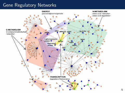
Gene Regulatory Networks
5
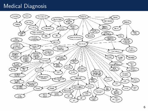
Medical Diagnosis
6
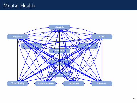
Mental Health
Anxiety
Depression
Paranoia
HallucinationsGrandiosity
Cognition
Physical Health
Worry
Insomnia Distress
PTSD
Dissociation
7
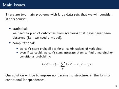
Main Issues
There are two main problems with large data sets that we will considerin this course:
• statistical;we need to predict outcomes from scenarios that have never beenobserved (i.e., we need a model).
• computational:
• we can’t store probabilities for all combinations of variables;• even if we could, we can’t sum/integrate them to find a marginal or
conditional probability:
P (X = x) =∑y
P (X = x,Y = y).
Our solution will be to impose nonparametric structure, in the form ofconditional independences.
8

Conditional Independence
9
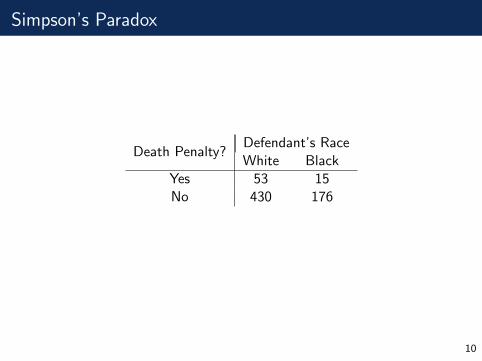
Simpson’s Paradox
Death Penalty?Defendant’s RaceWhite Black
Yes 53 15No 430 176
10
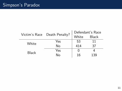
Simpson’s Paradox
Victim’s Race Death Penalty?Defendant’s RaceWhite Black
WhiteYes 53 11No 414 37
BlackYes 0 4No 16 139
11

Contingency Tables: Some Notation
We will consider multivariate systems of vectors XV ≡ (Xv : v ∈ V ) forsome set V = {1, . . . , p}.
Write XA ≡ (Xv : v ∈ A) for any A ⊆ V .
We assume that each Xv ∈ {1, . . . , dv} (usually dv = 2).
If we have n i.i.d. observations write
X(i)V ≡ (X
(i)1 , . . . , X(i)
p )T , i = 1, . . . , n.
12
Contingency Tables: Some Notation
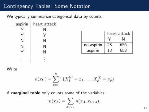
We typically summarize categorical data by counts:
aspirin heart attackY NY YN NN NY N...
...
heart attackY N
no aspirin 28 656aspirin 18 658
Write
n(xV ) =
n∑i=1
1{X(i)1 = x1, . . . , X
(i)p = xp}
A marginal table only counts some of the variables.
n(xA) =∑xV \A
n(xA, xV \A).
13

Marginal Table
Victim’s Race Death Penalty?Defendant’s RaceWhite Black
WhiteYes 53 11No 414 37
BlackYes 0 4No 16 139
If we sum out the Victim’s race...
Death Penalty?Defendant’s RaceWhite Black
Yes 53 15No 430 176
14

Contingency Tables
The death penalty data is on the class website.
> deathpen <- read.table("deathpen.txt", header=TRUE)
> deathpen
DeathPen Defendant Victim freq
1 Yes White White 53
2 No White White 414
3 Yes Black White 11
4 No Black White 37
5 Yes White Black 0
6 No White Black 16
7 Yes Black Black 4
8 No Black Black 139
15
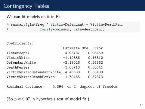
Contingency Tables
We can fit models on it in R:
> summary(glm(freq ~ Victim*Defendant + Victim*DeathPen,
+ family=poisson, data=deathpen))
Coefficients:
Estimate Std. Error
(Intercept) 4.93737 0.08459
VictimWhite -1.19886 0.16812
DefendantWhite -2.19026 0.26362
DeathPenYes -3.65713 0.50641
VictimWhite:DefendantWhite 4.46538 0.30408
VictimWhite:DeathPenYes 1.70455 0.52373
Residual deviance: 5.394 on 2 degrees of freedom
(So p ≈ 0.07 in hypothesis test of model fit.)
16
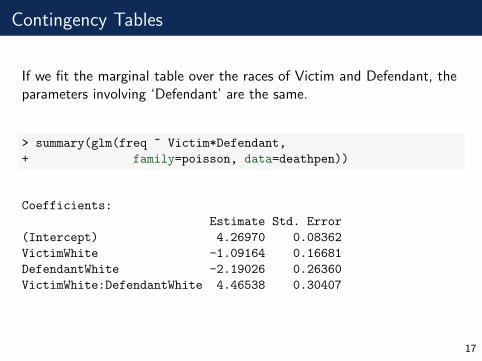
Contingency Tables
If we fit the marginal table over the races of Victim and Defendant, theparameters involving ‘Defendant’ are the same.
> summary(glm(freq ~ Victim*Defendant,
+ family=poisson, data=deathpen))
Coefficients:
Estimate Std. Error
(Intercept) 4.26970 0.08362
VictimWhite -1.09164 0.16681
DefendantWhite -2.19026 0.26360
VictimWhite:DefendantWhite 4.46538 0.30407
17

Undirected Graphical Models
18
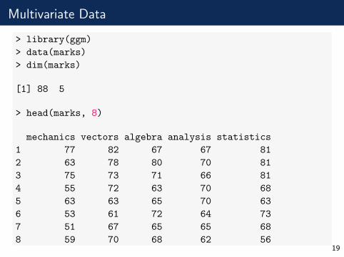
Multivariate Data
> library(ggm)
> data(marks)
> dim(marks)
[1] 88 5
> head(marks, 8)
mechanics vectors algebra analysis statistics
1 77 82 67 67 81
2 63 78 80 70 81
3 75 73 71 66 81
4 55 72 63 70 68
5 63 63 65 70 63
6 53 61 72 64 73
7 51 67 65 65 68
8 59 70 68 62 5619
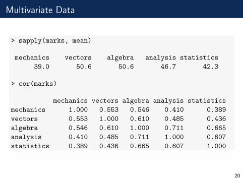
Multivariate Data
> sapply(marks, mean)
mechanics vectors algebra analysis statistics
39.0 50.6 50.6 46.7 42.3
> cor(marks)
mechanics vectors algebra analysis statistics
mechanics 1.000 0.553 0.546 0.410 0.389
vectors 0.553 1.000 0.610 0.485 0.436
algebra 0.546 0.610 1.000 0.711 0.665
analysis 0.410 0.485 0.711 1.000 0.607
statistics 0.389 0.436 0.665 0.607 1.000
20
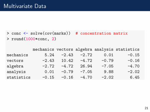
Multivariate Data
> conc <- solve(cov(marks)) # concentration matrix
> round(1000*conc, 2)
mechanics vectors algebra analysis statistics
mechanics 5.24 -2.43 -2.72 0.01 -0.15
vectors -2.43 10.42 -4.72 -0.79 -0.16
algebra -2.72 -4.72 26.94 -7.05 -4.70
analysis 0.01 -0.79 -7.05 9.88 -2.02
statistics -0.15 -0.16 -4.70 -2.02 6.45
21
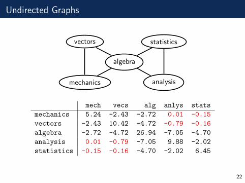
Undirected Graphs
algebra
vectors
mechanics
statistics
analysis
mech vecs alg anlys stats
mechanics 5.24 -2.43 -2.72 0.01 -0.15
vectors -2.43 10.42 -4.72 -0.79 -0.16
algebra -2.72 -4.72 26.94 -7.05 -4.70
analysis 0.01 -0.79 -7.05 9.88 -2.02
statistics -0.15 -0.16 -4.70 -2.02 6.45
22
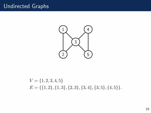
Undirected Graphs
3
1
2
4
5
V = {1, 2, 3, 4, 5}E = {{1, 2}, {1, 3}, {2, 3}, {3, 4}, {3, 5}, {4, 5}}.
23

Paths
3
1
2
4
5
Paths:
π1 : 1− 2− 3− 5
π2 : 3
Note that paths may consist of one vertex and no edges.
24

Induced Subgraph
3
1
2
4
5
The induced subgraph G{1,2,4,5} drops any edges that involve {3}.
25

Separation
3
1
2
4
5
All paths between {1, 2} and {5} pass through {3}.
Hence {1, 2} and {5} are separated by {3}.
26
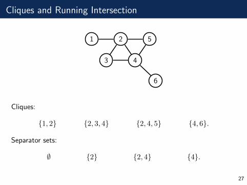
Cliques and Running Intersection
1 2
3 4
5
6
Cliques:
{1, 2} {2, 3, 4} {2, 4, 5} {4, 6}.
Separator sets:
∅ {2} {2, 4} {4}.
27
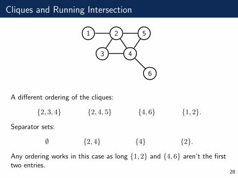
Cliques and Running Intersection
1 2
3 4
5
6
A different ordering of the cliques:
{2, 3, 4} {2, 4, 5} {4, 6} {1, 2}.
Separator sets:
∅ {2, 4} {4} {2}.
Any ordering works in this case as long {1, 2} and {4, 6} aren’t the firsttwo entries.
28
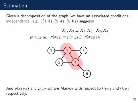
Estimation
Given a decomposition of the graph, we have an associated conditionalindependence: e.g. ({1, 3}, {2, 4}, {5, 6}) suggests
X1, X3 ⊥⊥ X5, X6 | X2, X4
p(x123456) · p(x24) = p(x1234) · p(x2456).
1 2
3 4
5
6
And p(x1234) and p(x2456) are Markov with respect to G1234 and G2456respectively.
29
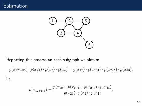
Estimation
1 2
3 4
5
6
Repeating this process on each subgraph we obtain:
p(x123456) · p(x24) · p(x2) · p(x4) = p(x12) · p(x234) · p(x245) · p(x46).
i.e.
p(x123456) =p(x12) · p(x234) · p(x245) · p(x46)
p(x24) · p(x2) · p(x4).
30

Non-Decomposable Graphs
But can’t we do this for any factorization?
1 2
34
No! Although
p(x1234) = ψ12(x12) · ψ23(x23) · ψ34(x34) · ψ14(x14),
the ψs are constrained by the requirement that∑x1234
p(x1234) = 1.
There is no nice representation of the ψCs in terms of p.31

Non-Decomposable Graphs
1 2
34
If we ‘decompose’ without a complete separator set then we introduceconstraints between the factors:
p(x1234) = p(x1 | x2, x4) · p(x3 | x2, x4),
but how to ensure that X2 ⊥⊥ X4 | X1, X3?
32

Iterative Proportional Fitting
33
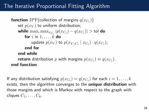
The Iterative Proportional Fitting Algorithm
function IPF(collection of margins q(xCi))set p(xV ) to uniform distribution;while maxi maxxCi
|p(xCi)− q(xCi)| > tol dofor i in 1, . . . , k do
update p(xV ) to p(xV \Ci| xCi) · q(xCi);
end forend whilereturn distribution p with margins p(xCi) ≈ q(xCi).
end function
If any distribution satisfying p(xCi) = q(xCi) for each i = 1, . . . , kexists, then the algorithm converges to the unique distribution withthose margins and which is Markov with respect to the graph withcliques C1, . . . , Ck.
34
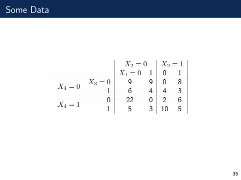
Some Data
X2 = 0 X2 = 1X1 = 0 1 0 1
X4 = 0X3 = 0 9 9 0 8
1 6 4 4 3
X4 = 10 22 0 2 61 5 3 10 5
35

Margins
Suppose we want to fit the 4-cycle model:
1 2
34
The relevant margins are:
n(x12) X2 = 0 1X1 = 0 42 16
1 16 22
n(x23) X3 = 0 1X2 = 0 40 18
1 16 22
n(x34) X4 = 0 1X3 = 0 26 30
1 17 23
n(x14) X4 = 0 1X1 = 0 19 39
1 24 14
36
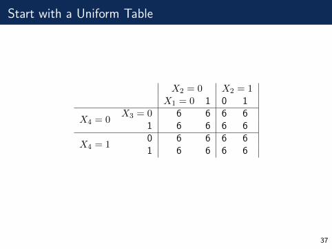
Start with a Uniform Table
X2 = 0 X2 = 1X1 = 0 1 0 1
X4 = 0X3 = 0 6 6 6 6
1 6 6 6 6
X4 = 10 6 6 6 61 6 6 6 6
37
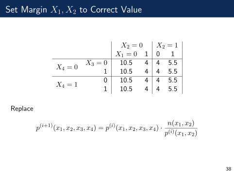
Set Margin X1, X2 to Correct Value
X2 = 0 X2 = 1X1 = 0 1 0 1
X4 = 0X3 = 0 10.5 4 4 5.5
1 10.5 4 4 5.5
X4 = 10 10.5 4 4 5.51 10.5 4 4 5.5
Replace
p(i+1)(x1, x2, x3, x4) = p(i)(x1, x2, x3, x4) ·n(x1, x2)
p(i)(x1, x2)
38
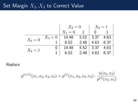
Set Margin X2, X3 to Correct Value
X2 = 0 X2 = 1X1 = 0 1 0 1
X4 = 0X3 = 0 14.48 5.52 3.37 4.63
1 6.52 2.48 4.63 6.37
X4 = 10 14.48 5.52 3.37 4.631 6.52 2.48 4.63 6.37
Replace
p(i+1)(x1, x2, x3, x4) = p(i)(x1, x2, x3, x4) ·n(x2, x3)
p(i)(x2, x3)
39
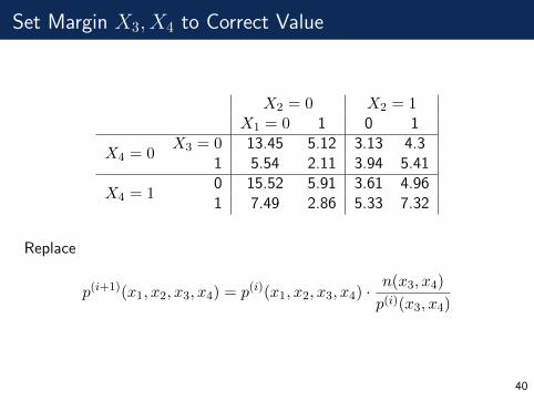
Set Margin X3, X4 to Correct Value
X2 = 0 X2 = 1X1 = 0 1 0 1
X4 = 0X3 = 0 13.45 5.12 3.13 4.3
1 5.54 2.11 3.94 5.41
X4 = 10 15.52 5.91 3.61 4.961 7.49 2.86 5.33 7.32
Replace
p(i+1)(x1, x2, x3, x4) = p(i)(x1, x2, x3, x4) ·n(x3, x4)
p(i)(x3, x4)
40
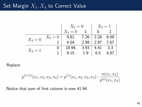
Set Margin X1, X4 to Correct Value
X2 = 0 X2 = 1X1 = 0 1 0 1
X4 = 0X3 = 0 9.81 7.26 2.28 6.09
1 4.04 2.99 2.87 7.67
X4 = 10 18.94 3.93 4.41 3.31 9.15 1.9 6.5 4.87
Replace
p(i+1)(x1, x2, x3, x4) = p(i)(x1, x2, x3, x4) ·n(x1, x4)
p(i)(x1, x4)
Notice that sum of first column is now 41.94.
41
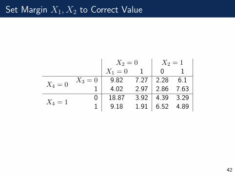
Set Margin X1, X2 to Correct Value
X2 = 0 X2 = 1X1 = 0 1 0 1
X4 = 0X3 = 0 9.82 7.27 2.28 6.1
1 4.02 2.97 2.86 7.63
X4 = 10 18.87 3.92 4.39 3.291 9.18 1.91 6.52 4.89
42
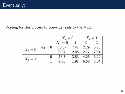
Eventually:
Waiting for this process to converge leads to the MLE:
X2 = 0 X2 = 1X1 = 0 1 0 1
X4 = 0X3 = 0 10.07 7.41 2.29 6.23
1 3.87 2.85 2.77 7.51
X4 = 10 18.7 3.83 4.26 3.221 9.36 1.91 6.68 5.04
43

Gaussian Graphical Models
44
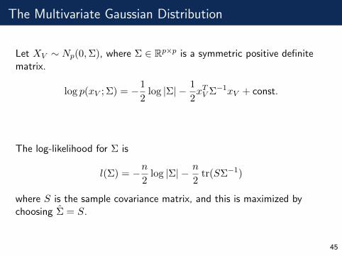
The Multivariate Gaussian Distribution
Let XV ∼ Np(0,Σ), where Σ ∈ Rp×p is a symmetric positive definitematrix.
log p(xV ; Σ) = −1
2log |Σ| − 1
2xTV Σ−1xV + const.
The log-likelihood for Σ is
l(Σ) = −n2
log |Σ| − n
2tr(SΣ−1)
where S is the sample covariance matrix, and this is maximized bychoosing Σ̂ = S.
45

Gaussian Graphical Models
We have Xa ⊥⊥ Xb | XV \{a,b} if and only if kab = 0.
analysis
algebra
statistics mechanics
vectors
mechanics vectors algebra analysis statisticsmechanics k11 k12 k13 0 0
vectors k22 k23 0 0algebra k33 k34 k35analysis k44 k45
statistics k55
46
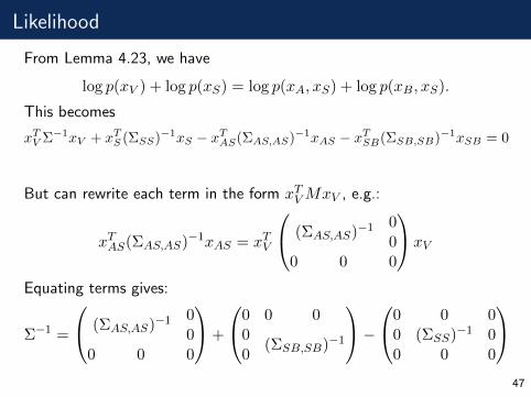
Likelihood
From Lemma 4.23, we have
log p(xV ) + log p(xS) = log p(xA, xS) + log p(xB, xS).
This becomes
xTV Σ−1xV + xTS (ΣSS)−1xS − xTAS(ΣAS,AS)−1xAS − xTSB(ΣSB,SB)−1xSB = 0
But can rewrite each term in the form xTVMxV , e.g.:
xTAS(ΣAS,AS)−1xAS = xTV
(ΣAS,AS)−100
0 0 0
xV
Equating terms gives:
Σ−1 =
(ΣAS,AS)−100
0 0 0
+
0 0 00
(ΣSB,SB)−10
−0 0 0
0 (ΣSS)−1 00 0 0
47
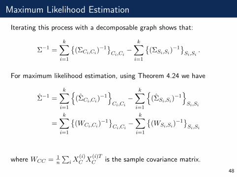
Maximum Likelihood Estimation
Iterating this process with a decomposable graph shows that:
Σ−1 =
k∑i=1
{(ΣCi,Ci)
−1}Ci,Ci
−k∑i=1
{(ΣSi,Si)
−1}Si,Si
.
For maximum likelihood estimation, using Theorem 4.24 we have
Σ̂−1 =
k∑i=1
{(Σ̂Ci,Ci)
−1}Ci,Ci
−k∑i=1
{(Σ̂Si,Si)
−1}Si,Si
=
k∑i=1
{(WCi,Ci)
−1}Ci,Ci
−k∑i=1
{(WSi,Si)
−1}Si,Si
where WCC = 1n
∑iX
(i)C X
(i)TC is the sample covariance matrix.
48
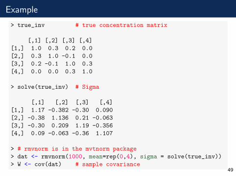
Example
> true_inv # true concentration matrix
[,1] [,2] [,3] [,4]
[1,] 1.0 0.3 0.2 0.0
[2,] 0.3 1.0 -0.1 0.0
[3,] 0.2 -0.1 1.0 0.3
[4,] 0.0 0.0 0.3 1.0
> solve(true_inv) # Sigma
[,1] [,2] [,3] [,4]
[1,] 1.17 -0.382 -0.30 0.090
[2,] -0.38 1.136 0.21 -0.063
[3,] -0.30 0.209 1.19 -0.356
[4,] 0.09 -0.063 -0.36 1.107
> # rmvnorm is in the mvtnorm package
> dat <- rmvnorm(1000, mean=rep(0,4), sigma = solve(true_inv))
> W <- cov(dat) # sample covariance49
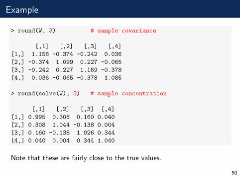
Example
> round(W, 3) # sample covariance
[,1] [,2] [,3] [,4]
[1,] 1.158 -0.374 -0.242 0.036
[2,] -0.374 1.099 0.227 -0.065
[3,] -0.242 0.227 1.169 -0.378
[4,] 0.036 -0.065 -0.378 1.085
> round(solve(W), 3) # sample concentration
[,1] [,2] [,3] [,4]
[1,] 0.995 0.308 0.160 0.040
[2,] 0.308 1.044 -0.138 0.004
[3,] 0.160 -0.138 1.026 0.344
[4,] 0.040 0.004 0.344 1.040
Note that these are fairly close to the true values.
50
Example
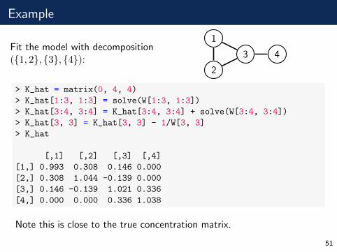
Fit the model with decomposition({1, 2}, {3}, {4}):
1
2
3 4
> K_hat = matrix(0, 4, 4)
> K_hat[1:3, 1:3] = solve(W[1:3, 1:3])
> K_hat[3:4, 3:4] = K_hat[3:4, 3:4] + solve(W[3:4, 3:4])
> K_hat[3, 3] = K_hat[3, 3] - 1/W[3, 3]
> K_hat
[,1] [,2] [,3] [,4]
[1,] 0.993 0.308 0.146 0.000
[2,] 0.308 1.044 -0.139 0.000
[3,] 0.146 -0.139 1.021 0.336
[4,] 0.000 0.000 0.336 1.038
Note this is close to the true concentration matrix.
51

Directed Graphical Models
52

Directed Graphs
The graphs considered so far are all undirected. Directed graphs giveeach edge an orientation.
A directed graph G is a pair (V,D), where
• V is a set of vertices;
• D is a set of ordered pairs (i, j) with i, j ∈ V and i 6= j.
If (i, j) ∈ D we write i→ j.
V = {1, 2, 3, 4, 5}D = {(1, 3), (2, 3), (2, 4), (3, 5), (4, 5)}.
If i→ j or i← j we say i andj are adjacent and writei ∼ j.
1 2
3 4
5
53

Acyclicity
Paths are sequences of adjacent vertices, without repetition:
1→ 3← 2→ 4→ 5 1→ 3→ 5.
The path is directed if all the arrows point away from the start.
(A path of length 0 is just a single vertex.)
A directed cycle is a directed path from i to j 6= i, together with j → i.
1 2
34
1
2
Graphs that contain no directed cycles are called acyclic. or morespecifically, directed acyclic graphs (DAGs).
All the directed graphs we consider are acyclic.54
Happy Families
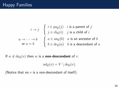
i→ j
{i ∈ paG(j) i is a parent of j
j ∈ chG(i) j is a child of i
a→ · · · → bor a = b
{a ∈ anG(b) a is an ancestor of b
b ∈ deG(a) b is a descendant of a
If w 6∈ deG(v) then w is a non-descendant of v:
ndG(v) = V \ deG(v).
(Notice that no v is a non-descendant of itself).
55
Examples
1 2
3 4
5
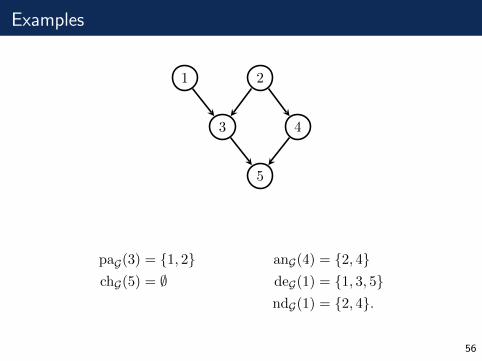
paG(3) = {1, 2} anG(4) = {2, 4}chG(5) = ∅ deG(1) = {1, 3, 5}
ndG(1) = {2, 4}.
56
Topological Orderings
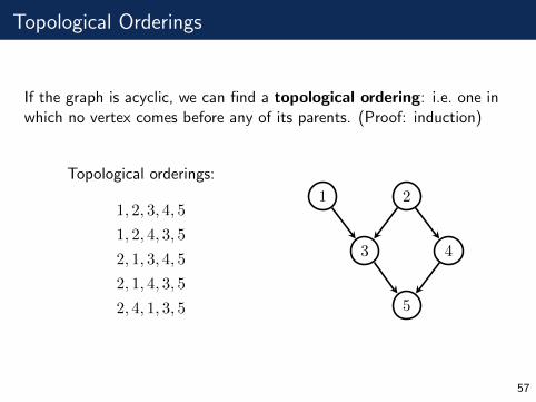
If the graph is acyclic, we can find a topological ordering: i.e. one inwhich no vertex comes before any of its parents. (Proof: induction)
Topological orderings:
1, 2, 3, 4, 5
1, 2, 4, 3, 5
2, 1, 3, 4, 5
2, 1, 4, 3, 5
2, 4, 1, 3, 5
1 2
3 4
5
57
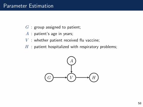
Parameter Estimation
G : group assigned to patient;
A : patient’s age in years;
V : whether patient received flu vaccine;
H : patient hospitalized with respiratory problems;
G V H
A
58
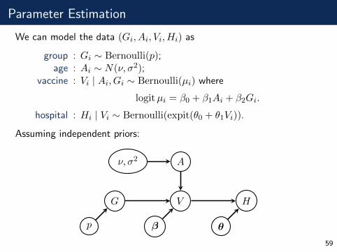
Parameter Estimation
We can model the data (Gi, Ai, Vi, Hi) as
group : Gi ∼ Bernoulli(p);age : Ai ∼ N(ν, σ2);
vaccine : Vi | Ai, Gi ∼ Bernoulli(µi) where
logitµi = β0 + β1Ai + β2Gi.
hospital : Hi | Vi ∼ Bernoulli(expit(θ0 + θ1Vi)).
Assuming independent priors:
G
p
V
β
H
θ
Aν, σ2
59
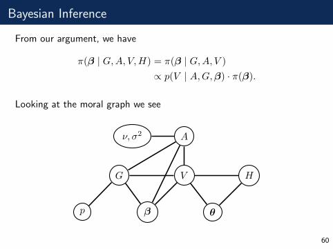
Bayesian Inference
From our argument, we have
π(β | G,A, V,H) = π(β | G,A, V )
∝ p(V | A,G,β) · π(β).
Looking at the moral graph we see
G
p
V
β
H
θ
Aν, σ2
60
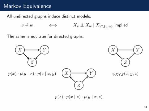
Markov Equivalence
All undirected graphs induce distinct models.
v 6∼ w ⇐⇒ Xv ⊥⊥ Xw | XV \{v,w} implied
The same is not true for directed graphs:
Z
X Y
p(x) · p(y | x) · p(z | x, y)
Z
X Y
p(z) · p(x | z) · p(y | x, z)
Z
X Y
ψXY Z(x, y, z)
61
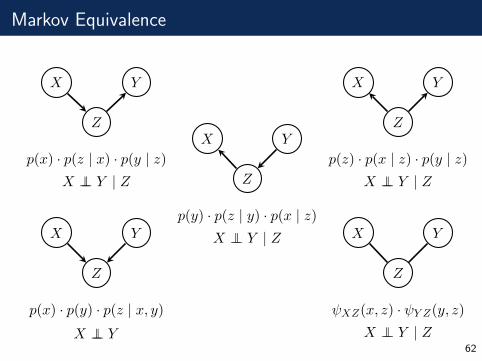
Markov Equivalence
Z
X Y
p(x) · p(z | x) · p(y | z)X ⊥⊥ Y | Z Z
X Y
p(y) · p(z | y) · p(x | z)X ⊥⊥ Y | Z
Z
X Y
p(z) · p(x | z) · p(y | z)X ⊥⊥ Y | Z
Z
X Y
p(x) · p(y) · p(z | x, y)
X ⊥⊥ Y
Z
X Y
ψXZ(x, z) · ψY Z(y, z)
X ⊥⊥ Y | Z62

Expert Systems
63
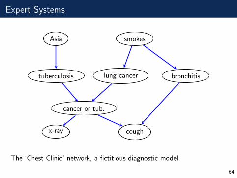
Expert Systems
Asia
tuberculosis lung cancer
smokes
bronchitis
cancer or tub.
x-ray cough
The ‘Chest Clinic’ network, a fictitious diagnostic model.
64
Variables
A
T L
S
B
E
XC
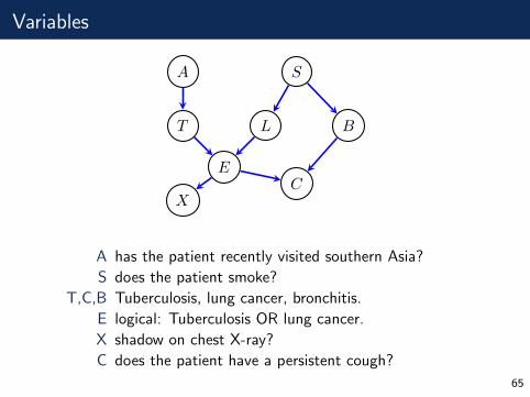
A has the patient recently visited southern Asia?
S does the patient smoke?
T,C,B Tuberculosis, lung cancer, bronchitis.
E logical: Tuberculosis OR lung cancer.
X shadow on chest X-ray?
C does the patient have a persistent cough?
65
Conditional Probability Tables
A
T L
S
B
E
XC
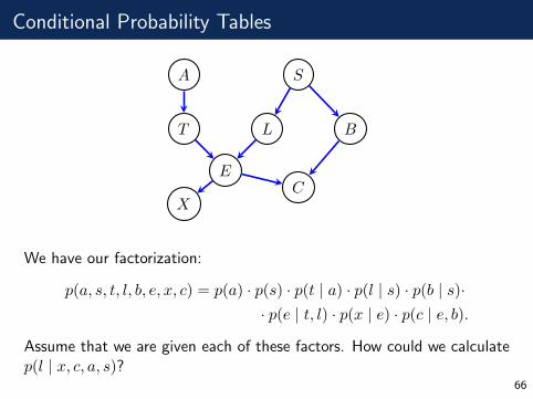
We have our factorization:
p(a, s, t, l, b, e, x, c) = p(a) · p(s) · p(t | a) · p(l | s) · p(b | s)·· p(e | t, l) · p(x | e) · p(c | e, b).
Assume that we are given each of these factors. How could we calculatep(l | x, c, a, s)?
66
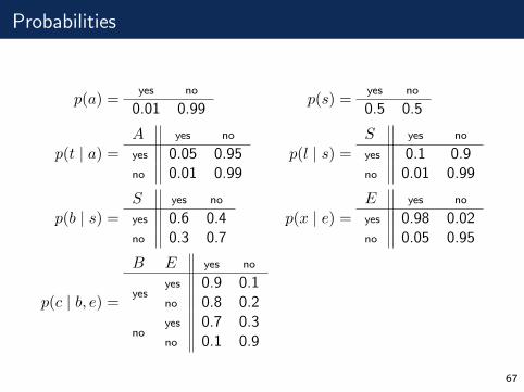
Probabilities
p(a) =yes no
0.01 0.99p(s) =
yes no
0.5 0.5
p(t | a) =A yes no
yes 0.05 0.95no 0.01 0.99
p(l | s) =S yes no
yes 0.1 0.9no 0.01 0.99
p(b | s) =S yes no
yes 0.6 0.4no 0.3 0.7
p(x | e) =E yes no
yes 0.98 0.02no 0.05 0.95
p(c | b, e) =
B E yes no
yesyes 0.9 0.1no 0.8 0.2
noyes 0.7 0.3no 0.1 0.9
67
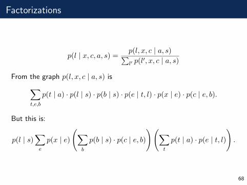
Factorizations
p(l | x, c, a, s) =p(l, x, c | a, s)∑l′ p(l
′, x, c | a, s)
From the graph p(l, x, c | a, s) is∑t,e,b
p(t | a) · p(l | s) · p(b | s) · p(e | t, l) · p(x | e) · p(c | e, b).
But this is:
p(l | s)∑e
p(x | e)
(∑b
p(b | s) · p(c | e, b)
)(∑t
p(t | a) · p(e | t, l)
).
68
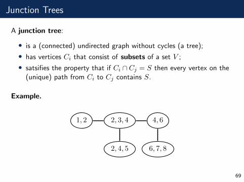
Junction Trees
A junction tree:
• is a (connected) undirected graph without cycles (a tree);
• has vertices Ci that consist of subsets of a set V ;
• satsifies the property that if Ci ∩ Cj = S then every vertex on the(unique) path from Ci to Cj contains S.
Example.
1, 2 2, 3, 4
2, 4, 5
4, 6
6, 7, 8
69
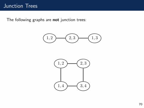
Junction Trees
The following graphs are not junction trees:
1, 2 2, 3 1, 3
1, 2 2, 3
3, 41, 4
70

Junction Trees
Junction trees can be constructed directly from sets of cliques satisfyingrunning intersection.
C1 C2
C3
C4C5
C6
Ci ∩⋃j<i
Cj = Ci ∩ Cσ(i).
71
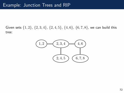
Example: Junction Trees and RIP
Given sets {1, 2}, {2, 3, 4}, {2, 4, 5}, {4, 6}, {6, 7, 8}, we can build thistree:
1, 2 2, 3, 4
2, 4, 5
4, 6
6, 7, 8
72
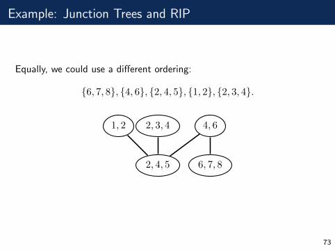
Example: Junction Trees and RIP
Equally, we could use a different ordering:
{6, 7, 8}, {4, 6}, {2, 4, 5}, {1, 2}, {2, 3, 4}.
6, 7, 8
4, 6
2, 4, 5
1, 2 2, 3, 4
73
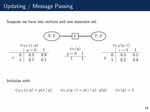
Updating / Message Passing
Suppose we have two vertices and one separator set.
X,Y Y Y, Z
ψXY (x, y)y = 0 1
x0 0.3 0.91 0.7 0.1
ψY (y)y = 0 1
1 1
ψY Z(y, z)z = 0 1
y0 0.3 0.11 0.2 0.4
Initialize with
ψXY (x, y) = p(x | y) ψY Z(y, z) = p(z | y) · p(y) ψY (y) = 1.
74
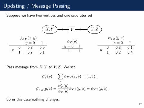
Updating / Message Passing
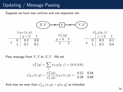
Suppose we have two vertices and one separator set.
X,Y Y Y, Z
ψXY (x, y)y = 0 1
x0 0.3 0.91 0.7 0.1
ψY (y)y = 0 1
1 1
ψY Z(y, z)z = 0 1
y0 0.3 0.11 0.2 0.4
Pass message from X,Y to Y,Z. We set
ψ′Y (y) =∑x
ψXY (x, y) = (1, 1);
ψ′Y Z(y, z) =ψ′Y (y)
ψY (y)ψY Z(y, z) = ψY Z(y, z).
So in this case nothing changes.75
Updating / Message Passing
Suppose we have two vertices and one separator set.
X,Y Y Y,Z
ψXY (x, y)y = 0 1
x0 0.3 0.91 0.7 0.1
ψ′Y (y)y = 0 1
1 1
ψ′Y Z(y, z)z = 0 1
y0 0.3 0.11 0.2 0.4
Pass message from Y,Z to X,Y . We set
ψ′′Y (y) =∑x
ψY Z(y, z) = (0.4, 0.6);
ψ′XY (x, y) =ψ′′Y (y)
ψ′Y (y)ψXY (x, y) =
0.12 0.540.28 0.06
.
And now we note that ψ′XY (x, y) = p(x, y) as intended.76
Rooting
1, 2 2, 3, 4
2, 4, 5
4, 6
6, 7, 8
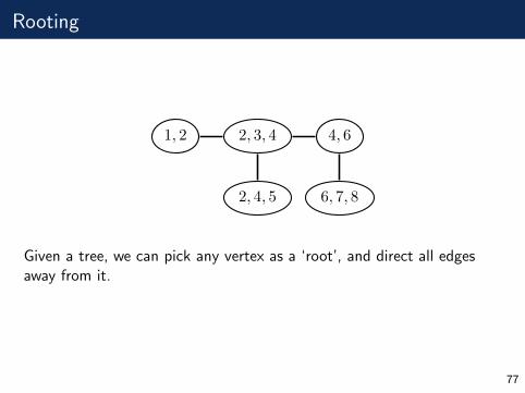
Given a tree, we can pick any vertex as a ‘root’, and direct all edgesaway from it.
77
Collection and Distribution
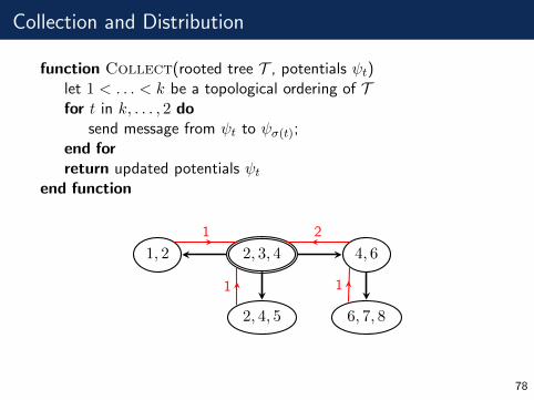
function Collect(rooted tree T , potentials ψt)let 1 < . . . < k be a topological ordering of Tfor t in k, . . . , 2 do
send message from ψt to ψσ(t);end forreturn updated potentials ψt
end function
1, 2 2, 3, 4
2, 4, 5
4, 6
6, 7, 8
1
1 1
2
78
Collection and Distribution
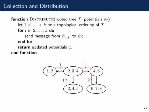
function Distribute(rooted tree T , potentials ψt)let 1 < . . . < k be a topological ordering of Tfor t in 2, . . . , k do
send message from ψσ(t) to ψt;end forreturn updated potentials ψt
end function
1, 2 2, 3, 4
2, 4, 5
4, 6
6, 7, 8
1
1
1
2
79
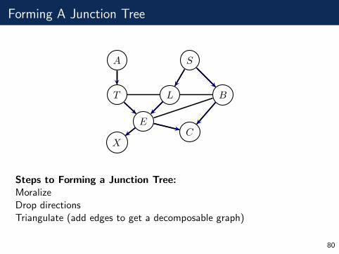
Forming A Junction Tree
A
T L
S
B
E
XC
Steps to Forming a Junction Tree:MoralizeDrop directionsTriangulate (add edges to get a decomposable graph)
80
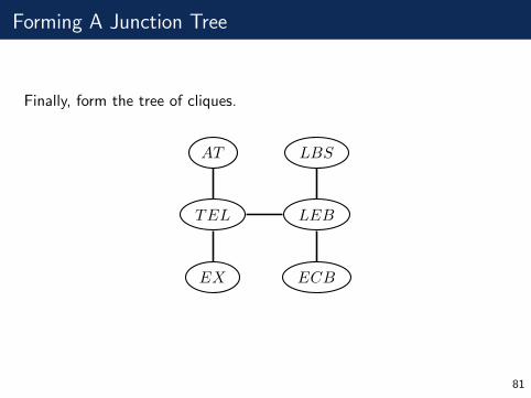
Forming A Junction Tree
Finally, form the tree of cliques.
LEBTEL
LBS
ECBEX
AT
81
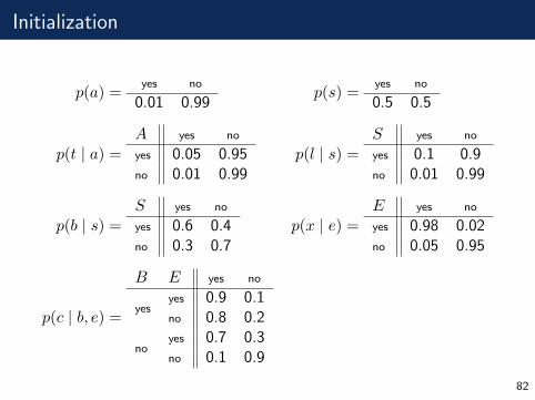
Initialization
p(a) =yes no
0.01 0.99p(s) =
yes no
0.5 0.5
p(t | a) =A yes no
yes 0.05 0.95no 0.01 0.99
p(l | s) =S yes no
yes 0.1 0.9no 0.01 0.99
p(b | s) =S yes no
yes 0.6 0.4no 0.3 0.7
p(x | e) =E yes no
yes 0.98 0.02no 0.05 0.95
p(c | b, e) =
B E yes no
yesyes 0.9 0.1no 0.8 0.2
noyes 0.7 0.3no 0.1 0.9
82
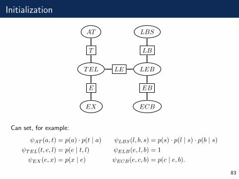
Initialization
LEBLETEL
LB
LBS
EB
ECB
E
EX
T
AT
Can set, for example:
ψAT (a, t) = p(a) · p(t | a) ψLBS(l, b, s) = p(s) · p(l | s) · p(b | s)ψTEL(t, e, l) = p(e | t, l) ψELB(e, l, b) = 1
ψEX(e, x) = p(x | e) ψECB(e, c, b) = p(c | e, b).
83
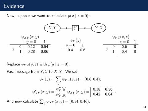
Evidence
Now, suppose we want to calculate p(x | z = 0).
X,Y Y Y,Z
ψXY (x, y)y = 0 1
x0 0.12 0.541 0.28 0.06
ψY (y)y = 0 1
0.4 0.6
ψY Z(y, z)z = 0 1
y0 0.6 01 0.4 0
Replace ψY Z(y, z) with p(y | z = 0).
Pass message from Y,Z to X,Y . We set
ψY (y) =∑x
ψY Z(y, z) = (0.6, 0.4);
ψ′XY (x, y) =ψ′′Y (y)
ψ′Y (y)ψXY (x, y) =
0.18 0.360.42 0.04
.
And now calculate∑
y ψXY (x, y) = (0.54, 0.46).
84
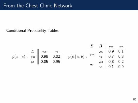
From the Chest Clinic Network
Conditional Probability Tables:
p(x | e) :E yes no
yes 0.98 0.02no 0.05 0.95
p(c | e, b) :
E B yes no
yesyes 0.9 0.1no 0.7 0.3
noyes 0.8 0.2no 0.1 0.9
85
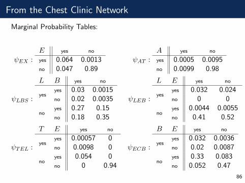
From the Chest Clinic Network
Marginal Probability Tables:
ψEX :E yes no
yes 0.064 0.0013no 0.047 0.89
ψAT :A yes no
yes 0.0005 0.0095no 0.0099 0.98
ψLBS :
L B yes no
yesyes 0.03 0.0015no 0.02 0.0035
noyes 0.27 0.15no 0.18 0.35
ψLEB :
L E yes no
yesyes 0.032 0.024no 0 0
noyes 0.0044 0.0055no 0.41 0.52
ψTEL :
T E yes no
yesyes 0.00057 0no 0.0098 0
noyes 0.054 0no 0 0.94
ψECB :
B E yes no
yesyes 0.032 0.0036no 0.02 0.0087
noyes 0.33 0.083no 0.052 0.47
86
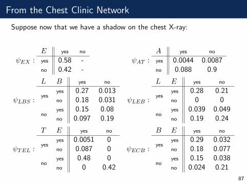
From the Chest Clinic Network
Suppose now that we have a shadow on the chest X-ray:
ψEX :E yes no
yes 0.58 -no 0.42 -
ψAT :A yes no
yes 0.0044 0.0087no 0.088 0.9
ψLBS :
L B yes no
yesyes 0.27 0.013no 0.18 0.031
noyes 0.15 0.08no 0.097 0.19
ψLEB :
L E yes no
yesyes 0.28 0.21no 0 0
noyes 0.039 0.049no 0.19 0.24
ψTEL :
T E yes no
yesyes 0.0051 0no 0.087 0
noyes 0.48 0no 0 0.42
ψECB :
B E yes no
yesyes 0.29 0.032no 0.18 0.077
noyes 0.15 0.038no 0.024 0.21
87
Causal Inference
88

Correlation
89
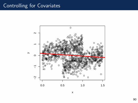
Controlling for Covariates
0.0 0.5 1.0 1.5
−2
−1
01
2
x
y
90
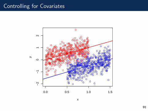
Controlling for Covariates
0.0 0.5 1.0 1.5
−2
−1
01
2
x
y
91
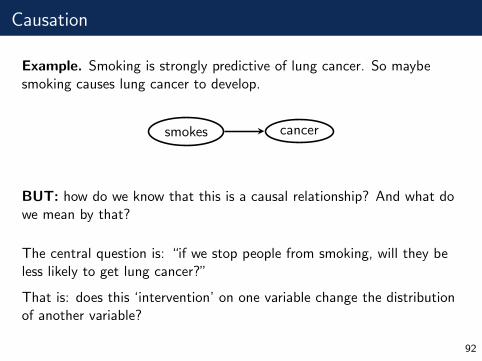
Causation
Example. Smoking is strongly predictive of lung cancer. So maybesmoking causes lung cancer to develop.
smokes cancer
BUT: how do we know that this is a causal relationship? And what dowe mean by that?
The central question is: “if we stop people from smoking, will they beless likely to get lung cancer?”
That is: does this ‘intervention’ on one variable change the distributionof another variable?
92
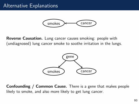
Alternative Explanations
smokes cancer
Reverse Causation. Lung cancer causes smoking: people with(undiagnosed) lung cancer smoke to soothe irritation in the lungs.
smokes cancer
gene
Confounding / Common Cause. There is a gene that makes peoplelikely to smoke, and also more likely to get lung cancer.
93
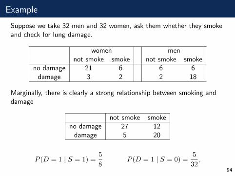
Example
Suppose we take 32 men and 32 women, ask them whether they smokeand check for lung damage.
women mennot smoke smoke not smoke smoke
no damage 21 6 6 6damage 3 2 2 18
Marginally, there is clearly a strong relationship between smoking anddamage
not smoke smokeno damage 27 12
damage 5 20
P (D = 1 | S = 1) =5
8P (D = 1 | S = 0) =
5
32.
94

Example
This might suggest that if we had prevented them all from smoking,only 5
32 × 64 = 10 would have had damage, whereas if we had madethem all smoke, 5
8 × 64 = 40 would have damage.
But: both smoking and damage are also correlated with gender, so thisestimate may be inaccurate. If we repeat this separately for men andwomen:
no-one smoking:
3
21 + 3× 32 +
2
6 + 2× 32 = 12
everyone smoking
2
6 + 2× 32 +
18
18 + 6× 32 = 32.
Compare these to 10 and 40.95
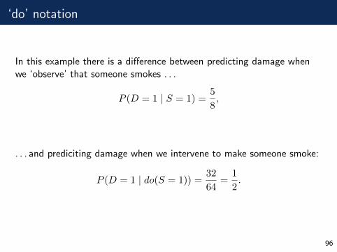
‘do’ notation
In this example there is a difference between predicting damage whenwe ‘observe’ that someone smokes . . .
P (D = 1 | S = 1) =5
8,
. . . and prediciting damage when we intervene to make someone smoke:
P (D = 1 | do(S = 1)) =32
64=
1
2.
96
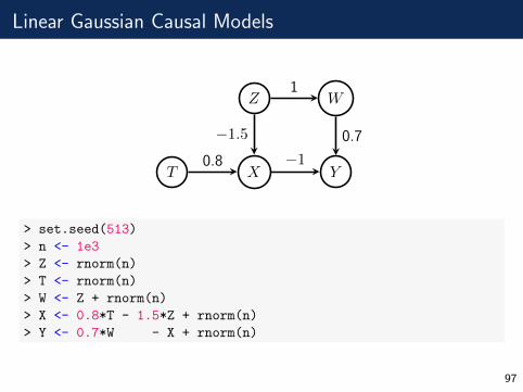
Linear Gaussian Causal Models
X
Z W
T Y0.8
−1.5
1
0.7
−1
> set.seed(513)
> n <- 1e3
> Z <- rnorm(n)
> T <- rnorm(n)
> W <- Z + rnorm(n)
> X <- 0.8*T - 1.5*Z + rnorm(n)
> Y <- 0.7*W - X + rnorm(n)
97
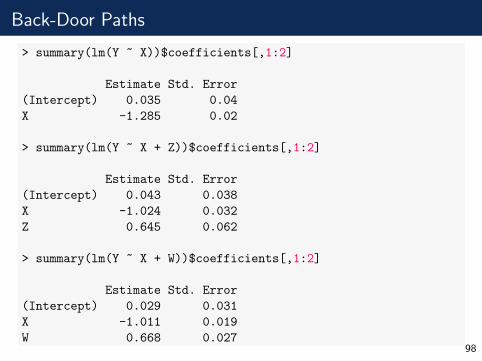
Back-Door Paths
> summary(lm(Y ~ X))$coefficients[,1:2]
Estimate Std. Error
(Intercept) 0.035 0.04
X -1.285 0.02
> summary(lm(Y ~ X + Z))$coefficients[,1:2]
Estimate Std. Error
(Intercept) 0.043 0.038
X -1.024 0.032
Z 0.645 0.062
> summary(lm(Y ~ X + W))$coefficients[,1:2]
Estimate Std. Error
(Intercept) 0.029 0.031
X -1.011 0.019
W 0.668 0.02798
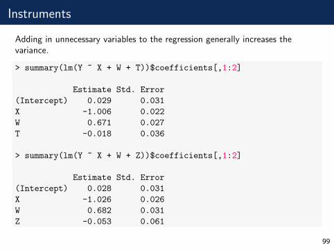
Instruments
Adding in unnecessary variables to the regression generally increases thevariance.
> summary(lm(Y ~ X + W + T))$coefficients[,1:2]
Estimate Std. Error
(Intercept) 0.029 0.031
X -1.006 0.022
W 0.671 0.027
T -0.018 0.036
> summary(lm(Y ~ X + W + Z))$coefficients[,1:2]
Estimate Std. Error
(Intercept) 0.028 0.031
X -1.026 0.026
W 0.682 0.031
Z -0.053 0.061
99
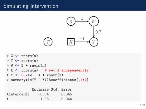
Simulating Intervention
X
Z W
T Y
1
0.7
−1
> Z <- rnorm(n)
> T <- rnorm(n)
> W <- Z + rnorm(n)
> X <- rnorm(n) # set X independently
> Y <- 0.7*W - X + rnorm(n)
> summary(lm(Y ~ X))$coefficients[,1:2]
Estimate Std. Error
(Intercept) -0.04 0.045
X -1.05 0.044
100
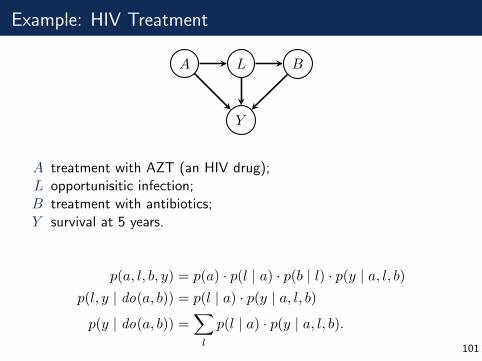
Example: HIV Treatment
A L B
Y
A treatment with AZT (an HIV drug);L opportunisitic infection;B treatment with antibiotics;Y survival at 5 years.
p(a, l, b, y) = p(a) · p(l | a) · p(b | l) · p(y | a, l, b)p(l, y | do(a, b)) = p(l | a) · p(y | a, l, b)
p(y | do(a, b)) =∑l
p(l | a) · p(y | a, l, b).101

Structural Equation Models
102

Covariance Matrices
Let G be a DAG with variables V .
X
Y
Zβ
γα
X = εx Y = αX + εy Z = βX + γY + εz.
XYZ
=
0 0 0α 0 0β γ 0
XYZ
+
εxεyεz
.
103

Covariance Matrices
Rearranging: 1 0 0−α 1 0−β −γ 1
XYZ
=
εxεyεz
.
Now, you can check that:
(I −B)−1 =
1 0 0−α 1 0−β −γ 1
−1 =
1 0 0α 1 0
β + αγ γ 1
,
so
Σ = (I −B)−1(I −B)−T
=
1 α β + αγα 1 + α2 αβ + γ + α2γ
β + αγ αβ + γ + α2γ 1 + γ2 + β2 + 2αβγ + α2γ2
.
104
Treks
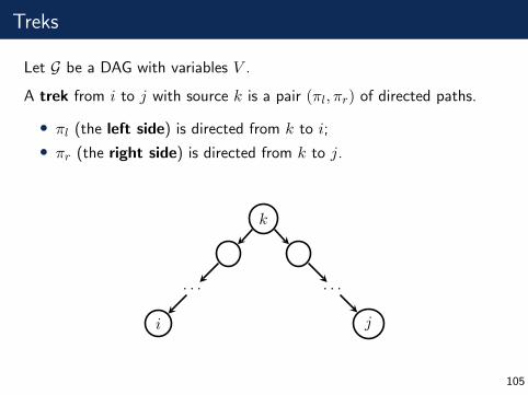
Let G be a DAG with variables V .
A trek from i to j with source k is a pair (πl, πr) of directed paths.
• πl (the left side) is directed from k to i;
• πr (the right side) is directed from k to j.
k
. . .
i
. . .
j
105

Trek Examples
Consider this DAG:
X
Y
Z
The treks from Z to Z are:
Z Z ← Y → Z
Z ← X → Z Z ← Y ← X → Z
Z ← X → Y → Z Z ← Y ← X → Y → Z.
Note that:
• A vertex may be in both the left and right sides.
• We may have i = k or j = k or both.
106

Treks
Let Σ be Markov with respect to a DAG G, so that
Σ = (I −B)−1D(I −B)−T .
Let τ = (πl, πr) be a trek with source k. The trek covarianceassociated with τ is:
c(τ) = dkk
∏(i→j)∈πl
bji
∏(i→j)∈πr
bji
.
107

Trek Covariance Examples
Consider this DAG:
X
Y
Zβ
γα
Trek covariances include:
c(Z) = 1 c(Z ← X) = β
c(Z ← X → Y → Z) = β · α · γ c(Y → Z) = γ.
Note that an empty product is 1 by convention.
108

Covariance Matrices
X
Y
Zβ
γα
Z Z ← Y → Z
Z ← X → Z Z ← Y ← X → Z
Z ← X → Y → Z Z ← Y ← X → Y → Z.
Recall that
σzz = 1 + γ2 + β2 + 2αβγ + α2γ2.
109

The Trek Rule
Theorem 8.15 (The Trek Rule)Let G be a DAG and let XV be Gaussian and Markov with respect to G.Then
σij =∑τ∈Tij
c(τ),
where Tij is the set of treks from i to j.
That is, the covariance between each Xi and Xj is the sum of the trekcovariances over all treks between i and j.
110

Gibbs Sampling
111

Gibbs Sampling
Suppose (X1
X2
)∼ N2
(0,
(1 ρρ 1
))so
K = Σ−1 =1
1− ρ2
(1 −ρ−ρ 1
).
Then
X1 | X2 = x2 ∼ N(ρx2, (1− ρ)2
)X2 | X1 = x1 ∼ N
(ρx1, (1− ρ)2
)
112
Gibbs Sampler
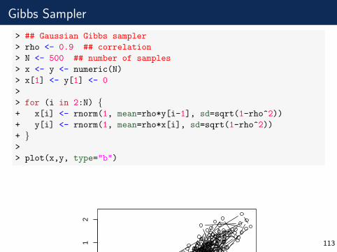
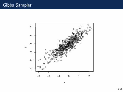
> ## Gaussian Gibbs sampler
> rho <- 0.9 ## correlation
> N <- 500 ## number of samples
> x <- y <- numeric(N)
> x[1] <- y[1] <- 0
>
> for (i in 2:N) {+ x[i] <- rnorm(1, mean=rho*y[i-1], sd=sqrt(1-rho^2))
+ y[i] <- rnorm(1, mean=rho*x[i], sd=sqrt(1-rho^2))
+ }>
> plot(x,y, type="b")
−3 −2 −1 0 1 2
−3
−2
−1
01
2
x
y
113

Gibbs Sampler
114
Gibbs Sampler
−3 −2 −1 0 1 2
−3
−2
−1
01
2
x
y
115
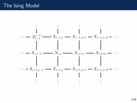
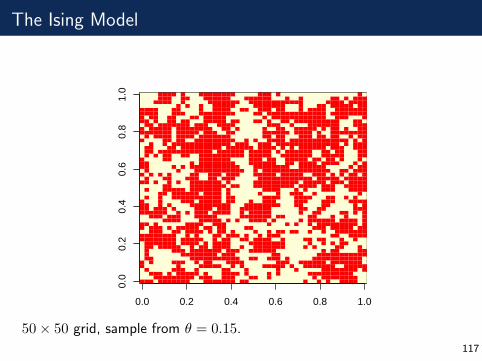
The Ising Model
Xj−1i−1 Xi−1,j Xi−1,j+1 Xi−1,j+2
Xi,j−1 Xi,j Xi,j+1 Xi,j+2
Xi+1,j−1 Xi+1,j Xi+1,j+1 Xi+1,j+2
· · · · · ·
......
......
· · · · · ·
· · · · · ·
......
......
116
The Ising Model
0.0 0.2 0.4 0.6 0.8 1.0
0.0
0.2
0.4
0.6
0.8
1.0
50× 50 grid, sample from θ = 0.15.
117
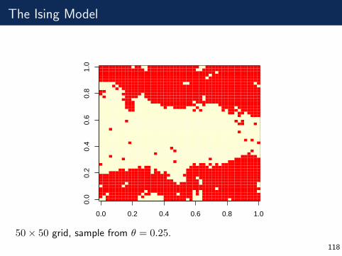
The Ising Model
0.0 0.2 0.4 0.6 0.8 1.0
0.0
0.2
0.4
0.6
0.8
1.0
50× 50 grid, sample from θ = 0.25.
118
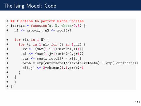
The Ising Model: Code
> ## function to perform Gibbs updates
> iterate = function(x, N, theta=0.5) {+ n1 <- nrow(x); n2 <- ncol(x)
+ for (it in 1:N) {+ for (i in 1:n1) for (j in 1:n2) {+ rw <- (max(1,i-1):min(n1,i+1))
+ cl <- (max(1,j-1):min(n2,j+1))
+ cur <- sum(x[rw,cl]) - x[i,j]
+ prob = exp(cur*theta)/c(exp(cur*theta) + exp(-cur*theta))
+ x[i,j] <- 2*rbinom(1,1,prob)-1
+ }+ }+ x
+ }
119
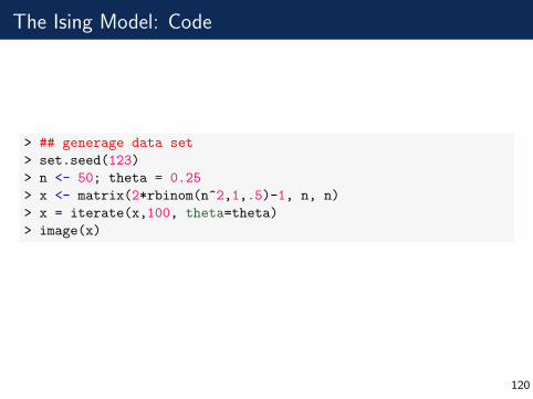
The Ising Model: Code
> ## generage data set
> set.seed(123)
> n <- 50; theta = 0.25
> x <- matrix(2*rbinom(n^2,1,.5)-1, n, n)
> x = iterate(x,100, theta=theta)
> image(x)
120

Introducing Evidence
Suppose that we know the border of the picture is all 1s.
> ## function to perform Gibbs updates
> iterate_border = function(x, N, theta=0.5) {+ n1 <- nrow(x); n2 <- ncol(x)
+ for (it in 1:N) {+ ## reduce scope of loop
+ for (i in 2:(n1-1)) for (j in 2:(n2-1)) {+ rw <- (max(1,i-1):min(n1,i+1))
+ cl <- (max(1,j-1):min(n2,j+1))
+ cur <- sum(x[rw,cl]) - x[i,j]
+ prob = exp(cur*theta)/c(exp(cur*theta) + exp(-cur*theta))
+ x[i,j] <- 2*rbinom(1,1,prob)-1
+ }+ }+ x
+ }
121
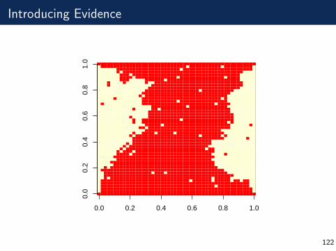
Introducing Evidence
0.0 0.2 0.4 0.6 0.8 1.0
0.0
0.2
0.4
0.6
0.8
1.0
122
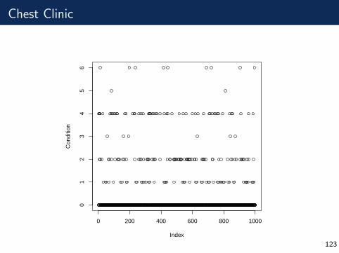
Chest Clinic
0 200 400 600 800 1000
01
23
45
6
Index
Con
ditio
n
123