satellite communication systems prof. kalyan kumar...

Satellite Communication Systems

Prof. Kalyan Kumar Bandyopadhyay

Department of Electronics and Electrical Communication Engineering

Indian Institute of Technology, Kharagpur

Lecture - 40

Satellite Navigation – II

Welcome back. So, we are talking of the satellite navigation and how to estimate the

position velocity and time and we started with position estimation in that we have seen

that it is coming as a quadratic equation. So, those ambiguities can be removed by a

simple technique of linearization. Where you have to have an approximate guess of your

position and then iterate and try to find out your position.

(Refer Slide Time: 00:41)

Now, like that you find out the position and with the iteration value and it can be seen

that it has been seen already, even if your initial guess is slightly away within 2, 3

iteration you will reach to the to your required position with sufficient accuracy required

accuracy.


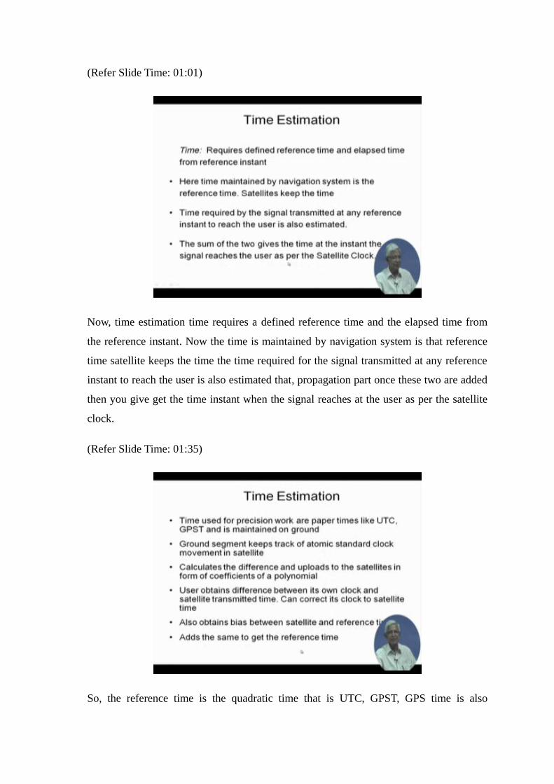
Now, time estimation time requires a defined reference time and the elapsed time from

the reference instant. Now the time is maintained by navigation system is that reference

time satellite keeps the time the time required for the signal transmitted at any reference

instant to reach the user is also estimated that, propagation part once these two are added

then you give get the time instant when the signal reaches at the user as per the satellite

clock.


So, the reference time is the quadratic time that is UTC, GPST, GPS time is also

maintained that is maintained on the ground and ground segment keeps the track of the

atomic clock standard and that atomic clock movement that small del t. So, that error and

it calculated the difference in upload the satellite in the form of coefficients of a

polynomial. So, that instead of correcting the clock on the satellite using additional

circuitry it simply sends a polynomial or the correction parameter. So, which will be

broadcasted to the user obtains a difference between it is own clock and the satellite

transmitted time and can correct the clock to the satellite time and also it ups obtains the

bias between satellite and the reference time which was modeled and uploaded and adds

the same to get the reference time.


That is how user gets the time velocity estimation is much simpler that is the pseudo

range rate can be found out from the Doppler. And the Doppler shift is pseudo range

divide by the wavelength and the pseudo range rate of the ith satellite can be expressed

can be found out in that form and that derivative form of our earlier quadratic equation.

So, in terms of range rates of satellite and user positions and time it can be found out this

can be solved using a set of four equations, similar way at the position determination are

maintained.


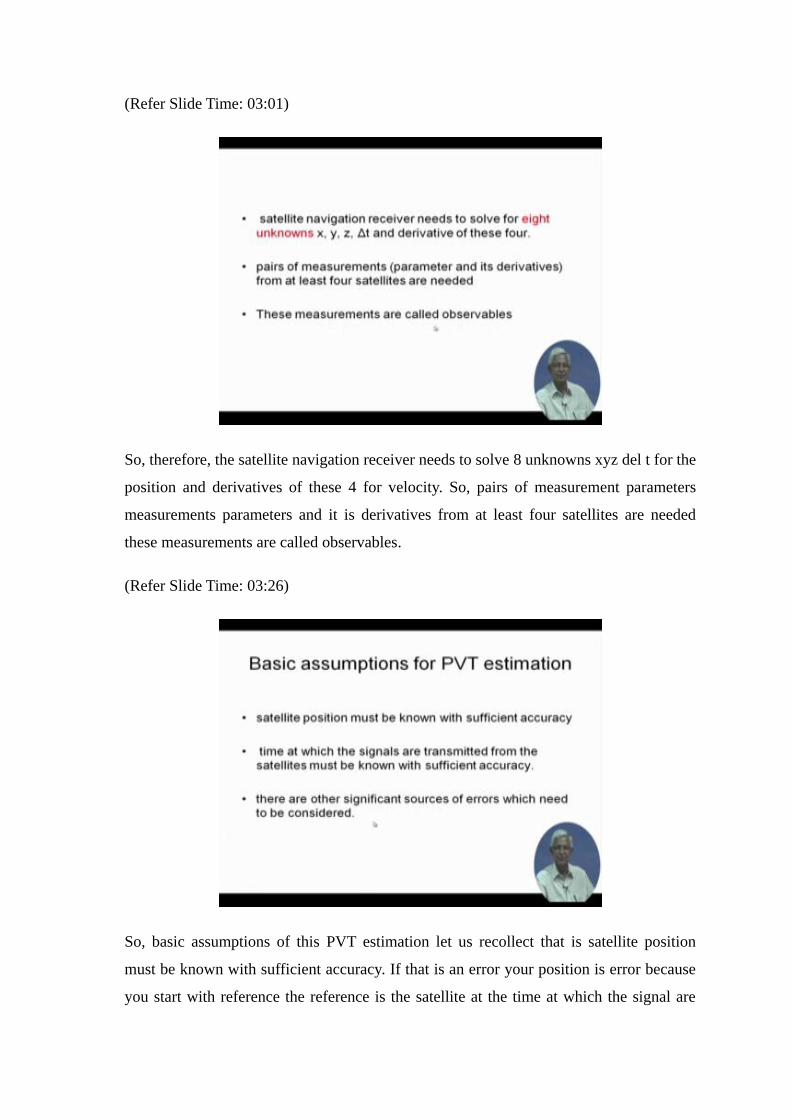
So, therefore, the satellite navigation receiver needs to solve 8 unknowns xyz del t for the

position and derivatives of these 4 for velocity. So, pairs of measurement parameters

measurements parameters and it is derivatives from at least four satellites are needed

these measurements are called observables.


So, basic assumptions of this PVT estimation let us recollect that is satellite position

must be known with sufficient accuracy. If that is an error your position is error because

you start with reference the reference is the satellite at the time at which the signal are

transmitted from the satellite must be known with sufficient accuracy. If that is an error

you are also in error because you are finding the range with respect to the time and the

propagation a time and there are other significant sources which need to be considered

we will see what are those different errors.


.

Now, let us go to the signal what is transmitted from the satellite that is GNSS that is

global navigation satellite system signal that consists of carrier power the navigational

data the ranging code the carrier frequency and phase and the it can be mathematically

expressed as let say y it i-th satellite i-th satellite signal is root 2 ci that is the amplitude

the d i t i stands for the i-th satellite d t ct and cos 2 pi f t plus phi where that root 2 ci is

the power component, the navigation data component is d i t navigation data which is

being broadcast which contains a satellite (Refer Time: 04:47) and other models and

other polynomials etcetera. The code is the ranging code c i t and that ranging code

consists of a PRN code unique for a satellite. So, satellites are identified by the PRN

code, instead of satellite number that provides the timing and the spreading, spectrum

spreading. So, all satellite use the CDMA mode of communication mostly that is (Refer

Time: 05:13) had FTMA, but they are changing over CDMA most of the all most all the

satellite navigation system are using CDMA modes mode of communication.

So, this is that ranging code which uses with the purpose of overlapping over the same

band width as well as unique identification of the particular satellite as well as time mark

and then the carrier frequency is fi and the phase is phi i.


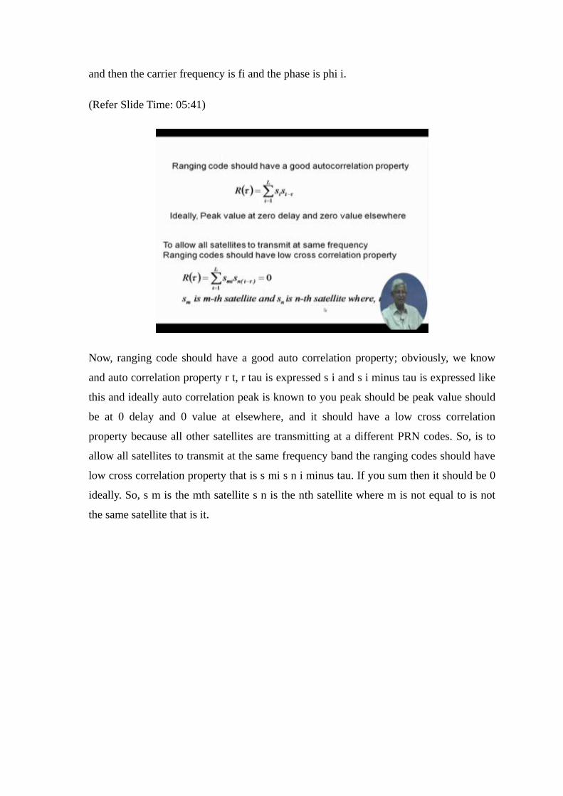
Now, ranging code should have a good auto correlation property; obviously, we know

and auto correlation property r t, r tau is expressed s i and s i minus tau is expressed like

this and ideally auto correlation peak is known to you peak should be peak value should

be at 0 delay and 0 value at elsewhere, and it should have a low cross correlation

property because all other satellites are transmitting at a different PRN codes. So, is to

allow all satellites to transmit at the same frequency band the ranging codes should have

low cross correlation property that is s mi s n i minus tau. If you sum then it should be 0

ideally. So, s m is the mth satellite s n is the nth satellite where m is not equal to is not

the same satellite that is it.


This is say a format in which the navigation message is transmitted it comes very slowly

you just see the 300 bit is of information at 50 bit is per second it takes 6 second to come

the complete message of 300 bit is and it is divided into many sub frames. So, each of

the sub frame TLM is telemetry how is hand over word then GPS week number when

first GPS was transmitted launched and service started from that weeks are counted. So,

how many weeks have elapsed then, satellite vehicle accuracy it is health clock

correction terms then, the sub frame 2 and 3 contains the ephemeris parameters of the

satellite and then, sub frame four contains the health data of satellite extra satellites

vehicles which are aw this is GPS actually. So, they have 24 satellites 25 to 30-32

satellites what are their health position special any other message ionospheric and UTC

data certain models also sent.

So, like that many other addition information are broadcast, but most important thing are

these 2 sub frame 2 and sub frame 2. Where the ephemeris are transmitted, as we are

seen that it is to be extracted separately and used.


Now, at the receiver the analog signal is delayed and Doppler is added satellites moving

where the user is also might be moving. So, Doppler is added to it. So, it is the same

equation from the all the satellites i equal to 1 to l let root over two ci it is di t minus tau

ci t minus tau. So, this tau is the delay whereas, reference f RF the frequency with on

which it transmit it is do Doppler delay by f d that ith 1 and then phi i.

So, that is the tau could delay and this is the Doppler. So, the receiver has to search not

only for the code to identify which, a satellite it is it has to also search for the Doppler.

So, it has a search space in that search space it is frequency beams as well as it has time

beams. So, digitized information which is available where the energy is maximum let us

say here this is the y it goes on searching goes on searching in frequency domain and

time domain and find out this.

So, it is a acquisition process is involved and once it is acquired it take some time to

acquire time to first acquire and after that it has to track that it because of Doppler it

might be moving the position, might be moving code delays are also changing. So,

therefore, it is acquisition and tracking both the functions are required in this process

needs a signal processing.


.

So, signal quality the demodulator should have adequate SNR and sir will do a quick

calculation try to see what the quality of the signal is for required this calculation is;

obviously, known to you the methods are known. Let us see CNR is estimated at the

receiver input and noise power primary depends on the input noise through the antenna

as well as the that is the noise figure of the receiver and the band width which is our ktb

that is noise power and let see t is 273 degree k 2 mega hertz which is a band width. So,

k is known. So, noise power is minus 141.2 dbw or 7.5 910 to the power minus 15 what

and the each signal is of the order 10 to the power minus 16 watt which is received at the

receiver from the satellite.

So, then 9 of the satellites assuming all of them are interfering with the same power. So,

9 times of this this is minus 150.5 dbw. So, noise plus interference CDMA is acting as a

interference noise plus interference in the numerical terms it those these values can be

added and you can get 8.5 into 10 to the power minus 15 watt which is minus 140.7 dbw

and your signal is minus 160 dbw that is 10 to the power minus 16. So, c by ni is minus

160 minus 140.7 is minus 19.3 db which is very low c by ni is lower CDMA has

received. So, which is of course, now the band width is 2 mega hertz is 63 db hertz here

and subtracted. So, c by n c by n plus i naught is minus 73.3 db hertz. So, CDMA gain

processing gain has to be 30 db with the processing gain of 30 db you get a minus 19.3

plus 30 is 10.7 db SNR at the correlator output you can you receive work up to that. So,

that is the CDMA advantage for your extracting output with a two mega bit is spreading

you gets 30 db correct just quick calculations.


.

Let us go back to our receiver block diagram is it has a antenna mostly Omni not need

not be fully Omni direction, but at least you should look at the sky. So, it is antenna and

the RF front end which has the RF amplifiers etcetera and then the after digitization it

does acquisition tracking which told you in search space and then once it is a data is

found out it goes into navigation processing it extracts the data tries to do that

linearization, find out it is position velocity and time.


Now, sources of error let us see what are the types of error that can come control error

which is the ephemeris error space error it is the satellite clock stability and clock code

bias and the propagation error is ionospheric propagation, delay tropospheric delay

multipath these are all variables and that the user receiver noise and receiver bias also

can have the control and space segment error is ephemeris and clock parameters

computed at the control segment and updated at certain intervals when it is visible to the

control station satellite is visible.


So, in between it will slightly drift. So, that is the control error errors in the estimation of

the parameter when you estimate that also there is a model. Because if that some error

may come this intermediate positions predicted using last updated data errors grow with

age for the prediction and there radial error is smallest along and cross track errors are

several times larger is etcetera.


Now, in the propagation path there is important thing which is ionospheric delay that is

ionosphere has different refractive index than, free space and electromagnetic wave

travels with lesser velocity than, free space hence using free space velocity of range for

ranging causes error and at this particular frequency normally which is allotted for this

satellite navigation which is one band then, ionosphere error is quite dominant at much

higher frequency it will much less and tropospheric delay is a dry and wet components

gases and vapors they also try to delay the signal.


So, therefore, there will be certain error scintillation is a phenomena which is a large

fluctuation of signal strength in short term that is formed by this small scale disturbance

in ionospheric that is electron or in tropospheric region by the gases etcetera. So, that

also affects something multipath is a fluctuation of signal strength due to the reflections

the incoherent combinations of the signals coming from different directions reflections

and scattering.


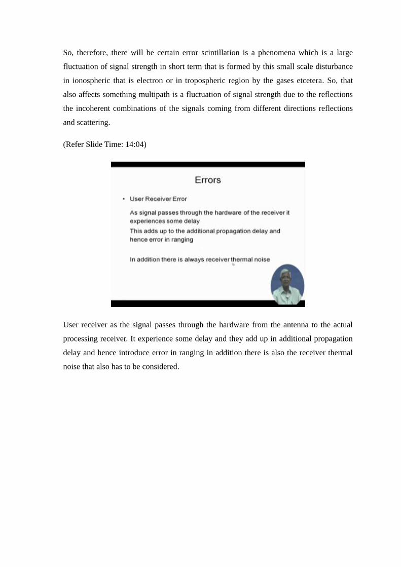
User receiver as the signal passes through the hardware from the antenna to the actual

processing receiver. It experience some delay and they add up in additional propagation

delay and hence introduce error in ranging in addition there is also the receiver thermal

noise that also has to be considered.


So, the true range if we call it capital r now they due to different errors the true range

from satellite receiver is not known exactly. So, this ratio pseudo range we have already

used this term.

So, pseudo range is the r plus the clock drift delay clock error iono, error a tropo error

and all other errors together.

So, now we have understood that there are certain errors and this has to be estimated

modeled or corrected how do you do that that is error correction is the wrong solution of

the position.


Unless the error terms are removed the correction error term can be done correction can

be done in 2 ways either by direct estimation estimate and model it and made use of

models or real time measurements all correction can be done with respect to a reference

receiver we which is called DGPS, differential GPS. Now direct estimation is clock bias

can be removed by the modeling of the clock movement and that can come through the

navigation message already, we have said that ionospheric errors can be single frequency

users can correct ionospheric errors using a model of the ionosphere at that location

because ionosphere varies at different places in the world dual frequency there are 2

frequency receivers can be there.


So, dual frequency users can calculate the ionospheric error and correct it because both

the frequency will have some similar type of error, that is coming in tropospheric error

can be used with within dry tropospheric model and receiver bias error can be changes

very slowly, but it has to be corrected it can be corrected by estimated a priori offline

measurement of the receiver bias and then, except the interval you can correct it

estimation may be updated at large interval.


The effect of error in measurement is ranges or ambiguous with certain width effect on

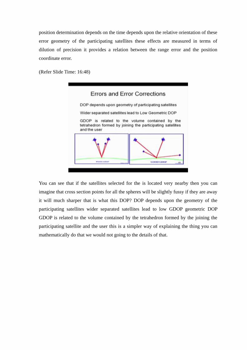
position determination depends on the time depends upon the relative orientation of these

error geometry of the participating satellites these effects are measured in terms of

dilution of precision it provides a relation between the range error and the position

coordinate error.


You can see that if the satellites selected for the is located very nearby then you can

imagine that cross section points for all the spheres will be slightly fussy if they are away

it will much sharper that is what this DOP? DOP depends upon the geometry of the

participating satellites wider separated satellites lead to low GDOP geometric DOP

GDOP is related to the volume contained by the tetrahedron formed by the joining the

participating satellite and the user this is a simpler way of explaining the thing you can

mathematically do that we would not going to the details of that.


Now, differential GPS techniques are used to reduce the position error using the

additional correction data from a reference GPS receiver situated at known position

previously known estimated well served point is known range error can be estimated at

the reference receiver estimated error be transmitted to the nearby user and these errors

are used for correction of the range of the user the error components, may be common to

the reference as well as the user it can be correlated or it is independent. Let us see I

mean DGPS does not receive a correct all the errors that is what is a meaning there are

three types of error components and cancellation of the range is leads to the accuracy.


So, how it is done there is a reference at this point which is ground reference well

surveyed point and there is a GPS receiver which is receiving from four satellites. Now if

user selects the same 4 satellites and he is getting the signal and user get some error since

this reference station knows it is own position it is well surveyed previously a priori

known. So, he knows what is the error it is getting from these four satellites; in these four

propagation path that error term he transmits to the user by another link. So, this

correction term comes and user corrects it, but as we said there are certain common

errors between these 2 reference station, as well as the user mobile user there are some

correlated terms and there are non correlated terms common errors are satellite

ephemeris error which is completely removed.

Because the same 4 satellites are selected correlated errors or the propagation errors if

they are closed by then the signals from these satellites to the reference as well as to the

mobile user are paths are more or less passing through the same part of the ionosphere

troposphere. So, they are can be assumed correlated if they are if they are closed by if

they are further having it cannot be removed. So, it can be therefore, it can be set

partially removed cancellation degrades with distance and non correlated errors multiples

will be different to the reference as well as the mobile user it can, cannot be removed at

all. So, differential GPS is not the full solution always, but it definitely improves.


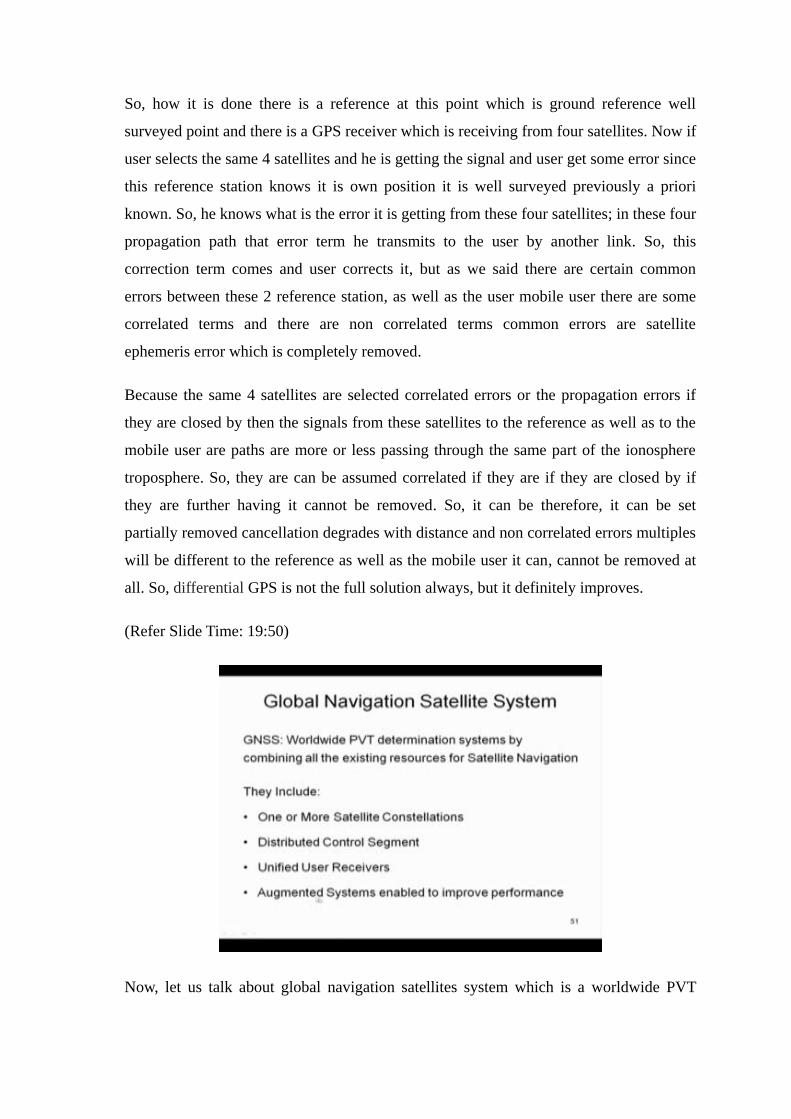
Now, let us talk about global navigation satellites system which is a worldwide PVT

determination system by combining all existing sources of the satellites navigation

people true to use GPS known as combined receiver Galileo GPS known as combined

receiver like that.

So, you have more number of satellites. So, you can select the best satellite looking at the

GDOP of different types of constellation satellites. So, one or more satellite

constellations are used distributed control segment unified user receiver and there are

augmented system enabled to improve the performance.


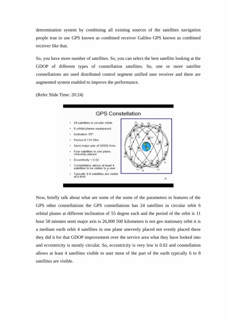
Now, briefly talk about what are some of the some of the parameters in features of the

GPS other constellations the GPS constellations has 24 satellites in circular orbit 6

orbital planes at different inclination of 55 degree each and the period of the orbit is 11

hour 58 minutes semi major axis is 26,000 500 kilometers is not geo stationary orbit it is

a medium earth orbit 4 satellites in one plane unevenly placed not evenly placed these

they did it for that GDOP improvement over the service area what they have looked into

and eccentricity is mostly circular. So, eccentricity is very low is 0.02 and constellation

allows at least 4 satellites visible to user most of the part of the earth typically 6 to 8

satellites are visible.


Another constellation GLONASS: Global Navigation Satellite System which is by

USSR, now it Russian republic it has also 24 satellites it has 3 orbital planes. Plane

separations are 120 degree 8 satellites per plane is also medium earth orbit 25,000

kilometer orbital period is 11 hour 15 minutes inclination is 64 degree at this inclination

is selected based on the their service area which is much higher latitude and there

transmit into 2 frequencies across.

Now, they have changed now this is a FDMA technique they have used and ranging

codes are this ca code is codes acquisition code and p code is precision code these are

also used by GPS at not mentioned in the earlier.


So, their frequencies are mentioned and modulation is FDMA, but now they are

changing over to CDMA Galileo with is European space agency is 27 plus there satellites

these 3 is extra satellites on orbit sphere and three orbital plane 120 degree separation of

the plane and 10 satellites per plane this is like a higher orbit 30,000 kilometer based on

again their requirement and 14 hours 22 minutes is orbital period inclination is 56 degree

and frequency is of 2 different transmissions are given and modulation is CDMA.

Now, in addition to that there are compass as well as other satellites India has launched

started launching it is own satellite which is regional satellite.


So, it is called Indian regional navigation satellite system IRNS must have seen the

announcements advertisements. Whenever they come up any satellites is launched

recently they have completed the constellations that is configuration is three geo satellite

you try to recollect it is geo stationary satellites.

So, their locations are known which are approximately 35 degree east 84 degrees east

and 130 degree east, it is a regional system. So, therefore, it is not covering whole earth

only covering only Indian region, India land mass as well as a surrounding ocean I mean

and nearby ocean area there are 4 GSO satellites they share geo synchronous satellites.

So, they have such an inclination you can imagine that tetrahedron all of the satellites if

they are on the same plane you would not get the proper GDOP. So, therefore, they are

has to be some satellites which are away from the equatorial plane. So, that is why this

inclinations given 4 satellites are there with 30 degree inclination at 55 degree distant

100 and 11 degree is across the equator that is total 7 satellites and there are master

control center has to be more than one. Because if one fails the other one takes place the

takes care and that range integrated monitoring system which is the required for the

control segment IRNSS RIMS are almost about 20 numbers I am not sure exact number

and there are command stations more than 5 numbers these are data I have collected just

sometimes back. So, may be may have a varied now.


So, we have mostly taken the reference of this linearization technique it is available in

many books and these here we have referred to the book which is understanding, GPS by

Kaplan. So, with this we have covered the what is meant by PVT and what is the

trilateration technique used in the satellite and the time and velocity how it is estimated

in addition to the position and then the basic functions of GNSS receiver very briefly you

can see it in PRATT also the book text book satellite communication. There also is

chapter there also you will get some of the information and errors and mitigation yeah

we talked D GPS and other module technique and some existing Sat Nav system. So,

with this we complete this satellite navigation which is has application of the satellite

communication.


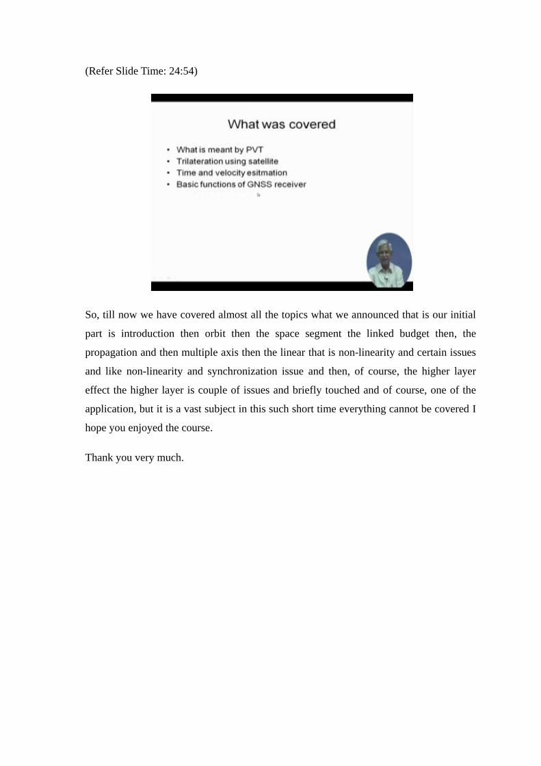
So, till now we have covered almost all the topics what we announced that is our initial

part is introduction then orbit then the space segment the linked budget then, the

propagation and then multiple axis then the linear that is non-linearity and certain issues

and like non-linearity and synchronization issue and then, of course, the higher layer

effect the higher layer is couple of issues and briefly touched and of course, one of the

application, but it is a vast subject in this such short time everything cannot be covered I

hope you enjoyed the course.

Thank you very much.

satellite communication systems prof. kalyan kumar...

Documents