sanders / van stee: algorithmentechnik january 30, 2008...
TRANSCRIPT

Sanders / van Stee: Algorithmentechnik January 30, 2008 1
Maximum Flows

Sanders / van Stee: Algorithmentechnik January 30, 2008 2
Definitions
¤ Network = directed weighted graph with source node s and sink
node t
¤ s has no incoming edges, t has no outgoing edges
¤ Weight ce of an edge e = capacity of e (nonnegative!)

Sanders / van Stee: Algorithmentechnik January 30, 2008 3
Definitions
¤ Flow = function fe on the edges, 0≤ fe ≤ ce∀eFor each node: total incoming flow = total outgoing flow
¤ Value of a flow = total outgoing flow from s
¤ Goal: find a flow with maximum value

Sanders / van Stee: Algorithmentechnik January 30, 2008 4
raaaaaaaaaaaaah
raaaaaaaaaaaaah

Sanders / van Stee: Algorithmentechnik January 30, 2008 5
Applications
¤ Oil pipes
¤ Traffic flows on highways
¤ Machine scheduling. Example:
Job 1 2 3 4
Size 1.5 1.25 2.1 3.6
Release date 3 1 3 5
Due date 5 4 7 9
Suppose we have three machines. Does a feasible schedule exist?

Sanders / van Stee: Algorithmentechnik January 30, 2008 6
Machine scheduling as a maxflow problem
¤ First layer of nodes contains the jobs
Each arc from s to a job has capacity equal to that job size
¤ Second layer of nodes contains intervals without release dates or
due dates
Arc from job to admissible interval I has capacity equal to length of
interval `(I)Arc from each interval to t has capacity 3`(I) = total amount of
work we can do in this interval (there are 3 machines)

Sanders / van Stee: Algorithmentechnik January 30, 2008 7
Matrix rounding
3.1 6.8 7.3 17.2
9.6 2.4 0.7 12.7
3.6 1.2 6.5 11.3
16.3 10.4 14.5
¤ Matrix with real numbers, column sums, row rums
¤ We can round each number up or down
¤ We want to get a consistent rounding
sum of rounded numbers in each row = rounded row sum

Sanders / van Stee: Algorithmentechnik January 30, 2008 8
Matrix rounding as a feasible flow problem
3.1 6.8 7.3 17.2
9.6 2.4 0.7 12.7
3.6 1.2 6.5 11.3
16.3 10.4 14.5
(14,15)
(10,11)(12,13)
(11,12)
(16,17)(17,18)
(3,4)
(6,7)
Feasible flow in this network = consistent rounding

Sanders / van Stee: Algorithmentechnik January 30, 2008 9
Feasible flow as a maxflow problem
Feasible circulation: for each
node i, incoming flow minus
outgoing flow = 0.
Upper and lower bounds on
flow on each arc
New flow variables: subtract
lower bound from all flow va-
riables and constraints
Now, for each node i, in-
coming flow minus outgoing
flow = b(i)
(14,15)
(10,11)(12,13)
(11,12)
(16,17)(17,18)
(3,4)
(6,7)
s t
8(0, )

Sanders / van Stee: Algorithmentechnik January 30, 2008 10
Feasible flow as a maxflow problem
Feasible circulation: for each
node i, incoming flow minus
outgoing flow = 0.
Upper and lower bounds on
flow on each arc
New flow variables: subtract
lower bound from all flow va-
riables
Now, for each node i, in-
coming flow minus outgoing
flow = b(i)
s t
8
1
1
1
1
1
1
1
1
1
40
−1
1
1 −1
−1
−40

Sanders / van Stee: Algorithmentechnik January 30, 2008 11
Feasible flow as a maxflow problem
¤ Add new sink s′ and new
source t ′
¤ For each node i with
b(i) > 0, add arc with
capacity b(i) from s′
¤ For each node i with
b(i) < 0, add arc with
capacity−b(i) to t ′
¤ Find maximum flow from
s′ to t ′
s’
t’
s t
8
1
1
1
1
1
1
1
40−40
−1
1
1 −1
−11
140
11
1
11
40 1

Sanders / van Stee: Algorithmentechnik January 30, 2008 12
Feasible flow as a maxflow problem
¤ If we find a flow that
saturates all source and
sink arcs, we have a fea-
sible flow in the original
network
¤ If the maximum flow
does not saturate those
edges, no feasible flow
exists!
s’
t’
s t
8
1
1
1
1
1
1
1
40−40
−1
1
1 −1
−11
140
11
1
11
40 1

Sanders / van Stee: Algorithmentechnik January 30, 2008 13
Option 1: linear programming
¤ Flow variables xe for each edge e
¤ Flow on each edge is at most its capacity
¤ Incoming flow at each vertex = outgoing flow from this vertex
¤ Maximize outgoing flow from starting vertex
We can do better!
Sanders / van Stee: Algorithmentechnik January 30, 2008 14
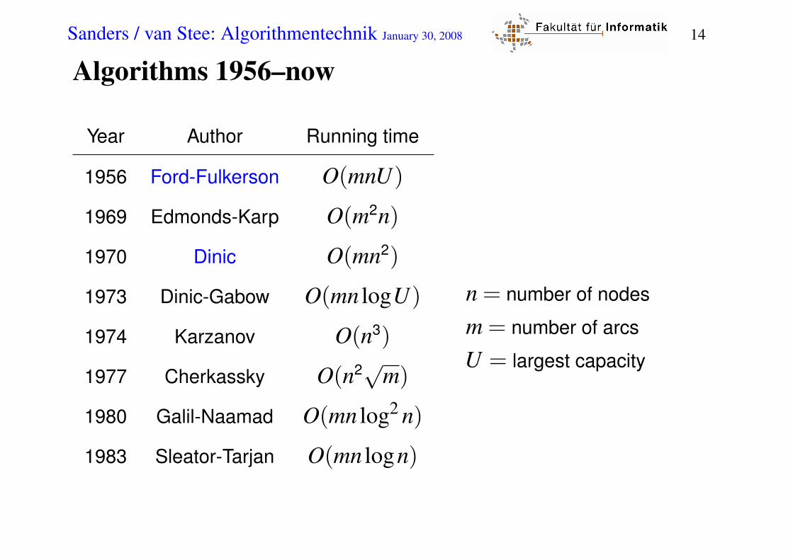
Algorithms 1956–now
Year Author Running time
1956 Ford-Fulkerson O(mnU)
1969 Edmonds-Karp O(m2n)
1970 Dinic O(mn2)
1973 Dinic-Gabow O(mn logU)
1974 Karzanov O(n3)
1977 Cherkassky O(n2√m)
1980 Galil-Naamad O(mn log2 n)
1983 Sleator-Tarjan O(mn logn)
n = number of nodes
m = number of arcs
U = largest capacity

Sanders / van Stee: Algorithmentechnik January 30, 2008 15
Year Author Running time
1986 Goldberg-Tarjan O(mn log(n2/m))
1987 Ahuja-Orlin O(mn+n2 logU)
1987 Ahuja-Orlin-Tarjan O(mn log(2+n√
logU/m))
1990 Cheriyan-Hagerup-Mehlhorn O(n3/ logn)
1990 Alon O(mn+n8/3 logn)
1992 King-Rao-Tarjan O(mn+n2+e)
1993 Philipps-Westbrook O(mn logn/ log mn +n2 log2+ε n)
1994 King-Rao-Tarjan O(mn logn/ log mn logn) if m≥ 2n logn
1997 Goldberg-Rao O(minm1/2,n2/3m log(n2/m) logU)

Sanders / van Stee: Algorithmentechnik January 30, 2008 16
Augmenting paths
Find a path from s to t such that each edge has some spare capacity
On this path, fill up the edge with the smallest spare capacity
Adjust capacities for all edges (create residual graph) and repeat

Sanders / van Stee: Algorithmentechnik January 30, 2008 17
Example
10
10
12
10
4
8
4
4

Sanders / van Stee: Algorithmentechnik January 30, 2008 18
Example
0
0
2
10
4
8
4
4
10
10
10
+10
Sanders / van Stee: Algorithmentechnik January 30, 2008 19
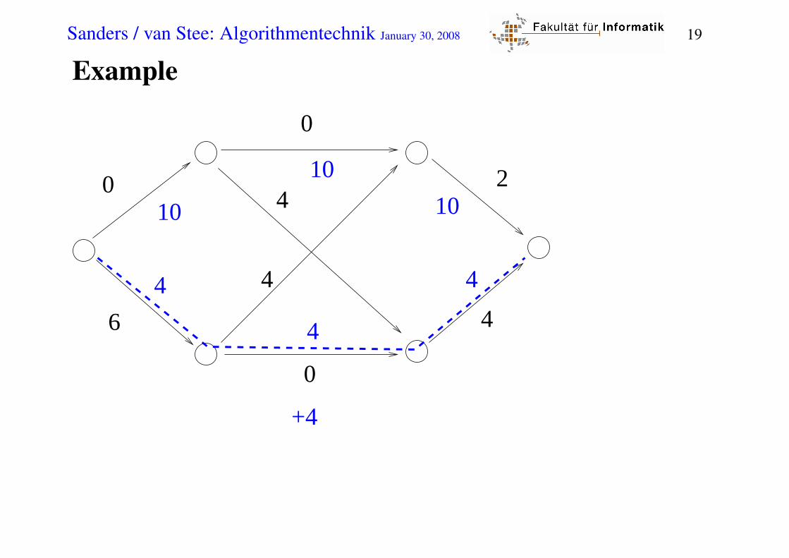
Example
0
0
2
6
0
4
4
4
10
10
10
4
4
4
+4
Sanders / van Stee: Algorithmentechnik January 30, 2008 20
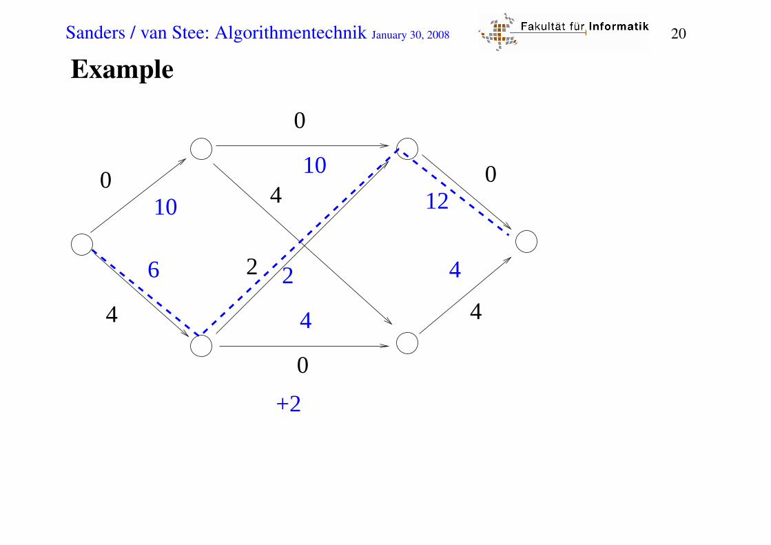
Example
0
0
0
4
0
4
4 10
10
12
6
4
42 2
+2
Sanders / van Stee: Algorithmentechnik January 30, 2008 21
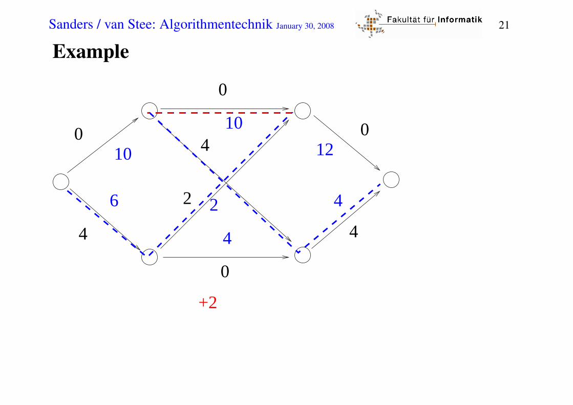
Example
0
0
0
4
0
4
4 10
10
12
6
4
42 2
+2
Sanders / van Stee: Algorithmentechnik January 30, 2008 22
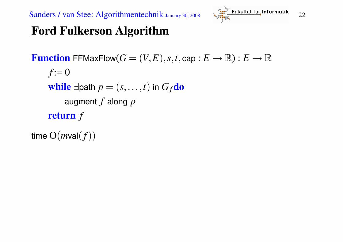
Ford Fulkerson Algorithm
Function FFMaxFlow(G = (V,E),s, t,cap : E → R) : E → Rf := 0while ∃path p = (s, . . . , t) in G f do
augment f along preturn f
time O(mval( f ))

Sanders / van Stee: Algorithmentechnik January 30, 2008 23
A Bad Example for Ford Fulkerson
100
100
100
100
1

Sanders / van Stee: Algorithmentechnik January 30, 2008 24
A Bad Example for Ford Fulkerson
100
100
100
100
1
99
100
100
99
1
1
1
1

Sanders / van Stee: Algorithmentechnik January 30, 2008 25
A Bad Example for Ford Fulkerson
100
100
100
100
1
99
100
100
99
1
99
99
99
99
1
1
1
1
1
1
0
1
1

Sanders / van Stee: Algorithmentechnik January 30, 2008 26
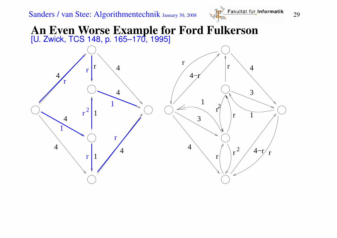
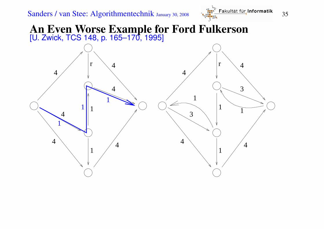
An Even Worse Example for Ford Fulkerson[U. Zwick, TCS 148, p. 165–170, 1995]
Let r =√
5−12
.
Consider the grapht
a
b
c
d
s
4 4
44
4 41
1
r
And the augmenting paths
p0 = 〈s,c,b, t〉p1 = 〈s,a,b,c,d, t〉p2 = 〈s,c,b,a, t〉p3 = 〈s,d,c,b, t〉The sequence of augmenting paths p0(p1, p2, p1, p3)∗ is an infinite
sequence of positive flow augmentations.
The flow value does not converge to the maximum value 9.

Sanders / van Stee: Algorithmentechnik January 30, 2008 27
An Even Worse Example for Ford Fulkerson[U. Zwick, TCS 148, p. 165–170, 1995]
4
r
4
3
44
14
1
r
4
4
4
44
1
1
11
31
11

Sanders / van Stee: Algorithmentechnik January 30, 2008 28
An Even Worse Example for Ford Fulkerson[U. Zwick, TCS 148, p. 165–170, 1995]
4
r
4
3
44
14
1
r
4
4
4
44
1
1
11
31
11
r
Sanders / van Stee: Algorithmentechnik January 30, 2008 29
An Even Worse Example for Ford Fulkerson[U. Zwick, TCS 148, p. 165–170, 1995]
4
r
4−r
3
4
4
1
r
4
4
4
44
1
1
1
31
1
r
r
r
r 2
r
rr2
rr2
4−r
r
r

Sanders / van Stee: Algorithmentechnik January 30, 2008 30
An Even Worse Example for Ford Fulkerson[U. Zwick, TCS 148, p. 165–170, 1995]
4
r
4−r
3
4
4
1
r
4
4
4
44
1
1
1
31
1
r
r
r
r 2
r
rr2
rr2
4−r
r
r
r

Sanders / van Stee: Algorithmentechnik January 30, 2008 31
An Even Worse Example for Ford Fulkerson[U. Zwick, TCS 148, p. 165–170, 1995]
4
r
4−r
3
4
4
1
r
4
4
4
44
1
1
1
31
1
r
r
r
1
rr2
4−r
r
r
1

Sanders / van Stee: Algorithmentechnik January 30, 2008 32
An Even Worse Example for Ford Fulkerson[U. Zwick, TCS 148, p. 165–170, 1995]
4
r
4−r
3
4
4
1
r
4
4
4
44
1
1
31
1
r
r
r
1
rr2
4−r
r
r
1
r r 2
1+r

Sanders / van Stee: Algorithmentechnik January 30, 2008 33
An Even Worse Example for Ford Fulkerson[U. Zwick, TCS 148, p. 165–170, 1995]
4
r
3
4−r
4
1
r
4
4
4
44
1
1
3
1
r+r
1 1
4−r−r
r+r
r+r
r
r
1 1−r2
2r
2
3
2
r+r2
2
2
4−r−r2
2
1−r2
1+r
2r

Sanders / van Stee: Algorithmentechnik January 30, 2008 34
An Even Worse Example for Ford Fulkerson[U. Zwick, TCS 148, p. 165–170, 1995]
4−r
r
3−r
4−r
4
1
r
4
4
4
44
1
1
3
1
r+r
r
r+r
1
4−r−r
r+r
r+r
r
r
1+r
2
3
1
2
r2
r2
21+r
1−r
4−r−r2
2
2
22
Sanders / van Stee: Algorithmentechnik January 30, 2008 35
An Even Worse Example for Ford Fulkerson[U. Zwick, TCS 148, p. 165–170, 1995]
4
r
4
3
44
14
1
r
4
4
4
44
1
1
11
31
11

Sanders / van Stee: Algorithmentechnik January 30, 2008 36
Blocking Flows
fb is a blocking flow in H if
∀paths p = 〈s, . . . , t〉 : ∃e ∈ p : fb(e) = cap(e)
s t
1/1
1/1
1/11/0
1/0

Sanders / van Stee: Algorithmentechnik January 30, 2008 37
Dinitz Algorithm
Function DinitzMaxFlow(G = (V,E),s, t,cap : E → R) : E → Rf := 0while ∃path p = (s, . . . , t) in G f do
d=G f .reverseBFS(t) : V → NL f = (V,
(u,v) ∈ E f : d(v) = d(u)−1
) // layer graph
find a blocking flow fb in L f
augment f += fb
return f

Sanders / van Stee: Algorithmentechnik January 30, 2008 38
Function blockingFlow(H = (V,E)) : E → Rp=〈s〉 : Path v=NodeRef : p.last()fb:= 0loop // Round
if v = t then // breakthroughδ := mincap(e)− fb(e) : e ∈ pforeach e ∈ p do
fb(e)+=δif fb(e) = cap(e) then remove e from E
p:= 〈s〉else if ∃e = (v,w) ∈ E then p.pushBack(w) // extendelse if v = s then return fb // doneelse delete the last edge from p in p and E // retreat

Sanders / van Stee: Algorithmentechnik January 30, 2008 39
Blocking Flows Analysis 1
¤ running time is #extends +#retreats +n ·#breakthroughs
¤ #breakthroughs ≤ m, since at least one edge is saturated
¤ #retreats ≤ m, since one edge is removed
¤ #extends ≤ #retreats +n ·#breakthroughs, since a retreat cancels one
extend and a breakthrough cancels n extends
time is O(m+nm) = O(nm)

Sanders / van Stee: Algorithmentechnik January 30, 2008 40
Blocking Flows Analysis 2
Unit capacities:
breakthroughs saturates all edges on p, i.e., amortized constant cost
per edge.
time O(m+n)
Sanders / van Stee: Algorithmentechnik January 30, 2008 41
Blocking Flows Analysis 3
Dynamic trees: breakthrough (!), retreat, extend in time O(logn)
time O((m+n) logn)
Theory alert: In practice, this seems to be slower (few breakthroughs,
many retreat, extend ops.)
Sanders / van Stee: Algorithmentechnik January 30, 2008 42
Dinitz Analysis 1
Lemma 1. d(s) increases by at least one in each round.
Beweis. not here
Sanders / van Stee: Algorithmentechnik January 30, 2008 43
Dinitz Analysis 2
¤ ≤ n rounds
¤ time O(mn) each
time O(mn2) (strongly polynomial)
time O(mn logn) with dynamic trees

Sanders / van Stee: Algorithmentechnik January 30, 2008 44
Dinitz Analysis 3
unit capacities
Lemma 2. At most 2√
m rounds:
Beweis. Consider round k =√
m.Any s-t path contains ≥ k edgesFF can find ≤ m/k =
√m augmenting paths
Total time: O((m+n)√
m)
more detailed analysis: O(
mmin
m1/2,n2/3)
∀v ∈V : minindegree(v),outdegree(v)= 1: time:
O((m+n)√
n)
Sanders / van Stee: Algorithmentechnik January 30, 2008 45
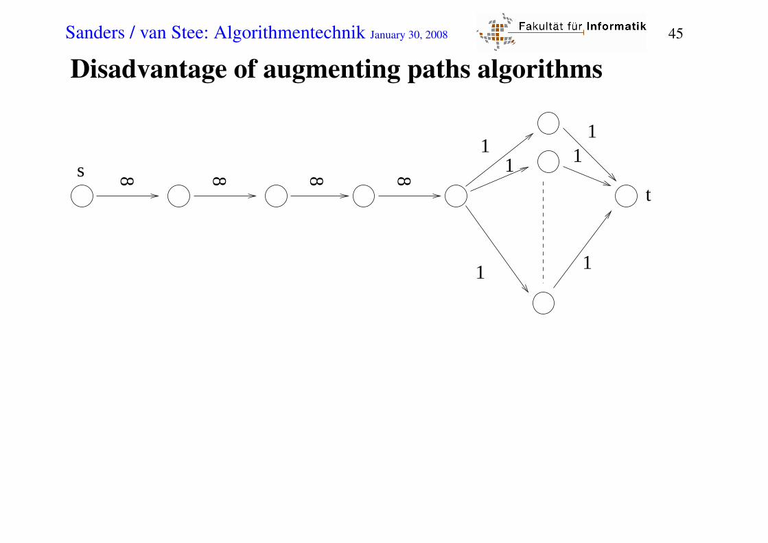
Disadvantage of augmenting paths algorithms
8 8 8 8
1
1
1
11
1
st

Sanders / van Stee: Algorithmentechnik January 30, 2008 46
Preflow-Push Algorithms
Preflow f : a flow where the flow conservation constraint is relaxed to
excess(v)≥ 0.
Procedure push(e = (v,w),δ )assert δ > 0assert residual capacity of e≥ δassert excess(v)≥ δexcess(v)−= δif f (e) > 0 then f (e)+ = δelse f (reverse(e))−= δ
Sanders / van Stee: Algorithmentechnik January 30, 2008 47
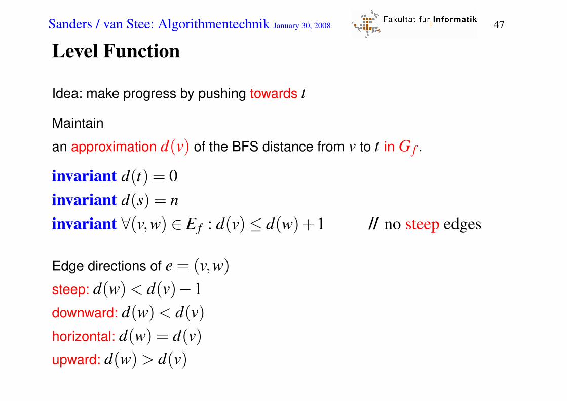
Level Function
Idea: make progress by pushing towards t
Maintain
an approximation d(v) of the BFS distance from v to t in G f .
invariant d(t) = 0invariant d(s) = ninvariant ∀(v,w) ∈ E f : d(v)≤ d(w)+1 // no steep edges
Edge directions of e = (v,w)steep: d(w) < d(v)−1downward: d(w) < d(v)horizontal: d(w) = d(v)upward: d(w) > d(v)

Sanders / van Stee: Algorithmentechnik January 30, 2008 48
Procedure genericPreflowPush(G=(V,E), f)
forall e = (s,v) ∈ E do push(e,cap(e)) // saturated(s):= nd(v):= 0 for all other nodes
while ∃v ∈V \s, t : excess(v) > 0 do // active nodeif ∃e = (v,w) ∈ E f : d(w) < d(v) then // eligible edge
choose some δ ≤minexcess(v), resCap(e)push(e,δ ) // no new steep edges
else d(v)++ // relabel. No new steep edges
Obvious choice for δ : δ = minexcess(v), resCap(e)Saturating push: δ = resCap(e)nonsaturating push: δ < resCap(e)
To be filled in: How to select active nodes and eligible edges?

Sanders / van Stee: Algorithmentechnik January 30, 2008 49
Lemma 3.∀ active nodes v : excess(v) > 0⇒∃ path 〈v, . . . ,s〉 ∈ G f
Intuition: what got there can always go back.
Beweis. S :=
u ∈V : ∃ path 〈v, . . .u〉 ∈ G f
, T := V \S. Then
∑u∈S
excess(u) = ∑e∈E∩(T×S)
f (e)− ∑e∈E∩(S×T )
f (e),
∀(u,w) ∈ E f : u ∈ S⇒ w ∈ S by Def. of G f , S⇒∀e = (u,w) ∈ E ∩ (T ×S) : f (e) = 0 Otherwise (w,u) ∈ E f
Hence, ∑u∈S
excess(u)≤ 0
One the negative excess of s can outweigh excess(v) > 0.Hence s ∈ S.

Sanders / van Stee: Algorithmentechnik January 30, 2008 50
Lemma 3.∀ active nodes v : excess(v) > 0⇒∃ path 〈v, . . . ,s〉 ∈ G f
Intuition: what got there can always go back.
Beweis. S :=
u ∈V : ∃ path 〈v, . . .u〉 ∈ G f
, T := V \S. Then
∑u∈S
excess(u) = ∑e∈E∩(T×S)
f (e)− ∑e∈E∩(S×T )
f (e),
∀(u,w) ∈ E f : u ∈ S⇒ w ∈ S by Def. of G f , S⇒∀e = (u,w) ∈ E ∩ (T ×S) : f (e) = 0 Otherwise (w,u) ∈ E f
Hence, ∑u∈S
excess(u)≤ 0
One the negative excess of s can outweigh excess(v) > 0.Hence s ∈ S.

Sanders / van Stee: Algorithmentechnik January 30, 2008 51
Lemma 4.∀v ∈V : d(v) < 2n
Beweis. Suppose v is lifted to d(v) = 2n.By Lemma 3, there is a (simple) path p to s in G f .p has at most n−1 nodesd(s) = n.Hence d(v) < 2n. Contradiction.

Sanders / van Stee: Algorithmentechnik January 30, 2008 52
Partial Correctness
Lemma 5. When genericPreflowPush terminates f is a maximalflow.
Beweis.f is a flow since ∀v ∈V \s, t : excess(v) = 0.
To show that f is maximal, it suffices to show that6 ∃ path p = 〈s, . . . , t〉 ∈ G f (Max-Flow Min-Cut Theorem):Since d(s) = n, d(t) = 0, p would have to contain steep edges.That would be a contradiction.
Sanders / van Stee: Algorithmentechnik January 30, 2008 53
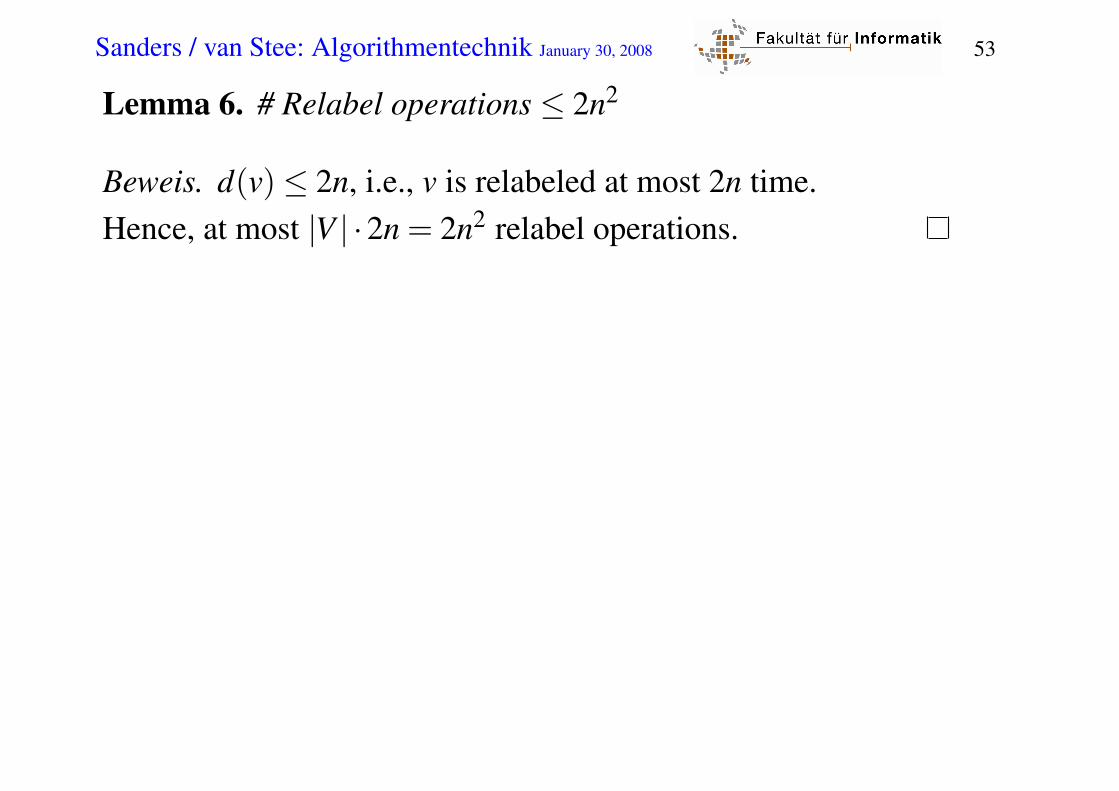
Lemma 6. # Relabel operations ≤ 2n2
Beweis. d(v)≤ 2n, i.e., v is relabeled at most 2n time.Hence, at most |V | ·2n = 2n2 relabel operations.
Sanders / van Stee: Algorithmentechnik January 30, 2008 54
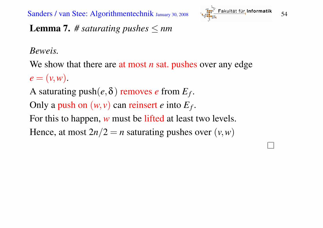
Lemma 7. # saturating pushes ≤ nm
Beweis.We show that there are at most n sat. pushes over any edgee = (v,w).A saturating push(e,δ ) removes e from E f .Only a push on (w,v) can reinsert e into E f .For this to happen, w must be lifted at least two levels.Hence, at most 2n/2 = n saturating pushes over (v,w)

Sanders / van Stee: Algorithmentechnik January 30, 2008 55
Lemma 8. # nonsaturating pushes = O(n2m
)
if δ = minexcess(v), resCap(e)for arbitrary node and edge selection rules.(arbitrary-preflow-push)
Beweis. Φ := ∑v:v is active
d(v). (Potential)
Φ = 0 initially and at the end (no active nodes left!)
Operation ∆(Φ) How many times? Total effect
relabel 1 ≤ 2n2 ≤ 2n2
saturating push ≤ 2n ≤ nm ≤ 2n2m
nonsaturating push ≤−1
Φ≥ 0 always.
Sanders / van Stee: Algorithmentechnik January 30, 2008 56
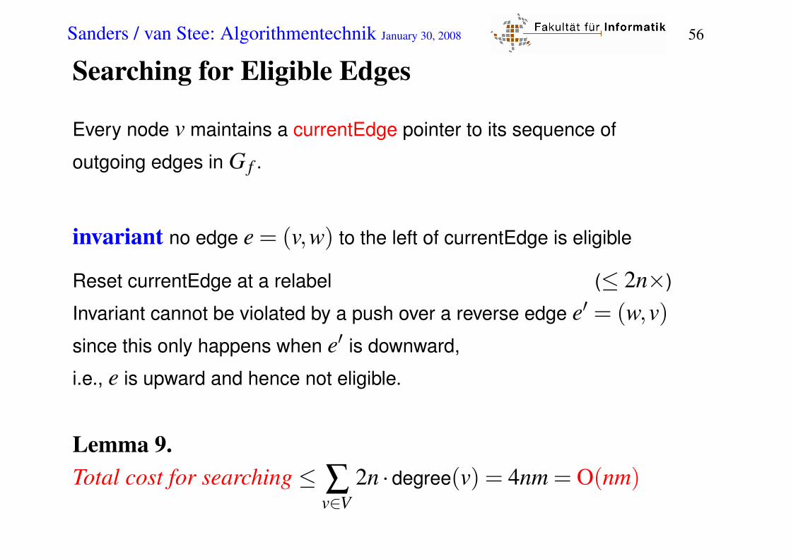
Searching for Eligible Edges
Every node v maintains a currentEdge pointer to its sequence of
outgoing edges in G f .
invariant no edge e = (v,w) to the left of currentEdge is eligible
Reset currentEdge at a relabel (≤ 2n×)
Invariant cannot be violated by a push over a reverse edge e′ = (w,v)since this only happens when e′ is downward,
i.e., e is upward and hence not eligible.
Lemma 9.Total cost for searching ≤ ∑
v∈V2n · degree(v) = 4nm = O(nm)

Sanders / van Stee: Algorithmentechnik January 30, 2008 57
Satz 10. Arbitrary Preflow Push finds a maximum flow in timeO
(n2m
).
Beweis.Lemma 5: partial correctnessInitialization in time O(n+m).Maintain set (e.g., stack, FIFO) of active nodes.Use reverse edge pointers to implement push.Lemma 6: 2n2 relabel operationsLemma 7: nm saturating pushesLemma 8: O
(n2m
)nonsaturating pushes
Lemma 9: O(nm) search time for eligible edges———————————————————————–Total time O
(n2m
)

Sanders / van Stee: Algorithmentechnik January 30, 2008 58
FIFO Preflow push
Examine active nodes in first-in, first-out order
Node examination = sequence of saturating pushes followed by
nonsaturating push or relabel
e=15
7
3
11
8
e=0
7
3
8
56
saturating
nonsaturatingpush
pushes

Sanders / van Stee: Algorithmentechnik January 30, 2008 59
FIFO Preflow push
Examine active nodes in first-in, first-out order
Node examination = sequence of saturating pushes followed by
nonsaturating push or relabel
Partition sequence of examinations into phases
Phase 1 = examination of nodes that became active in preprocessing
Phase 2 = examination of nodes that became active in phase 1
. . .
Phase i = examination of nodes that became active in phase i−1
At most n nonsaturating pushes per phase. But how many phases?
Sanders / van Stee: Algorithmentechnik January 30, 2008 60
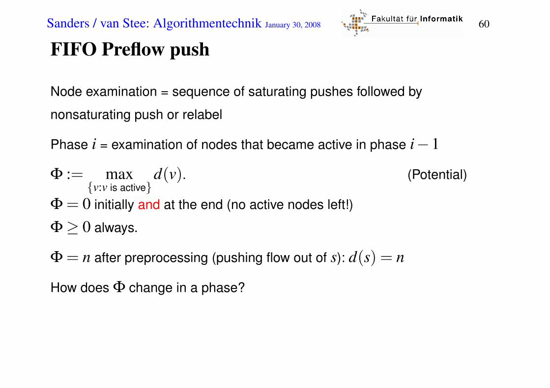
FIFO Preflow push
Node examination = sequence of saturating pushes followed by
nonsaturating push or relabel
Phase i = examination of nodes that became active in phase i−1
Φ := maxv:v is active
d(v). (Potential)
Φ = 0 initially and at the end (no active nodes left!)
Φ≥ 0 always.
Φ = n after preprocessing (pushing flow out of s): d(s) = n
How does Φ change in a phase?

Sanders / van Stee: Algorithmentechnik January 30, 2008 61
FIFO Preflow push
Φ := maxv:v is active
d(v). (Potential)
¤ At least one relabel operation in a phase:
∆(Φ)≤ maximum increase of any distance label
Total increase in Φ over all phases≤ 2n2
¤ No relabel operation:
all excess moves to nodes with smaller distance labels
Φ decreases by at least 1
There cannot be more than 2n2 +n phases before Φ = 0No active nodes left⇒ FIFO-PP runs in O
(n3)

Sanders / van Stee: Algorithmentechnik January 30, 2008 62
Modified FIFO preflow push
FIFO: examine nodes in FIFO order
MFIFO: when a node is relabeled, put it first in the list
MFIFO does not leave a node until all excess is pushed out of it
(FIFO leaves a node when it is relabeled)
e=15
7
3
8
e=0
7
3
4
saturatingpushes
d=5
d=4
d=4
d=4
d=5
11d=6
4

Sanders / van Stee: Algorithmentechnik January 30, 2008 63
Bucket-Queues
Eine Bucket-Queue ist ein kreisförmi-
ges Array B von C + 1 doppelt gelink-
ten Listen
Ein Knoten mit aktuelle Distanz d[v]wird gespeichert bei Index
d[v] mod (C +1)
Alle Knoten im gleichen Bucket haben
die gleiche Distanz d[v]!
a, 29 b, 30 30c,
d, 31
e, 33
f, 35
g, 36
01
23
456
7
89
min
mod 10
Bucket queue with C = 9
<(a,29), (b,30), (c,30), (d,31)
(e,33), (f,35), (g,36)>
Content=

Sanders / van Stee: Algorithmentechnik January 30, 2008 64
Highest Level Preflow Push
Always select active nodes that maximize d(v)Use bucket priority queue (insert, increaseKey, deleteMax)
not monotone (!) but relabels “pay” for scan operations
Lemma 11. At most n2√m nonsaturating pushes.
Beweis. later
Satz 12. Highest Level Preflow Push finds a maximum flow intime O
(n2√m
).
Sanders / van Stee: Algorithmentechnik January 30, 2008 65
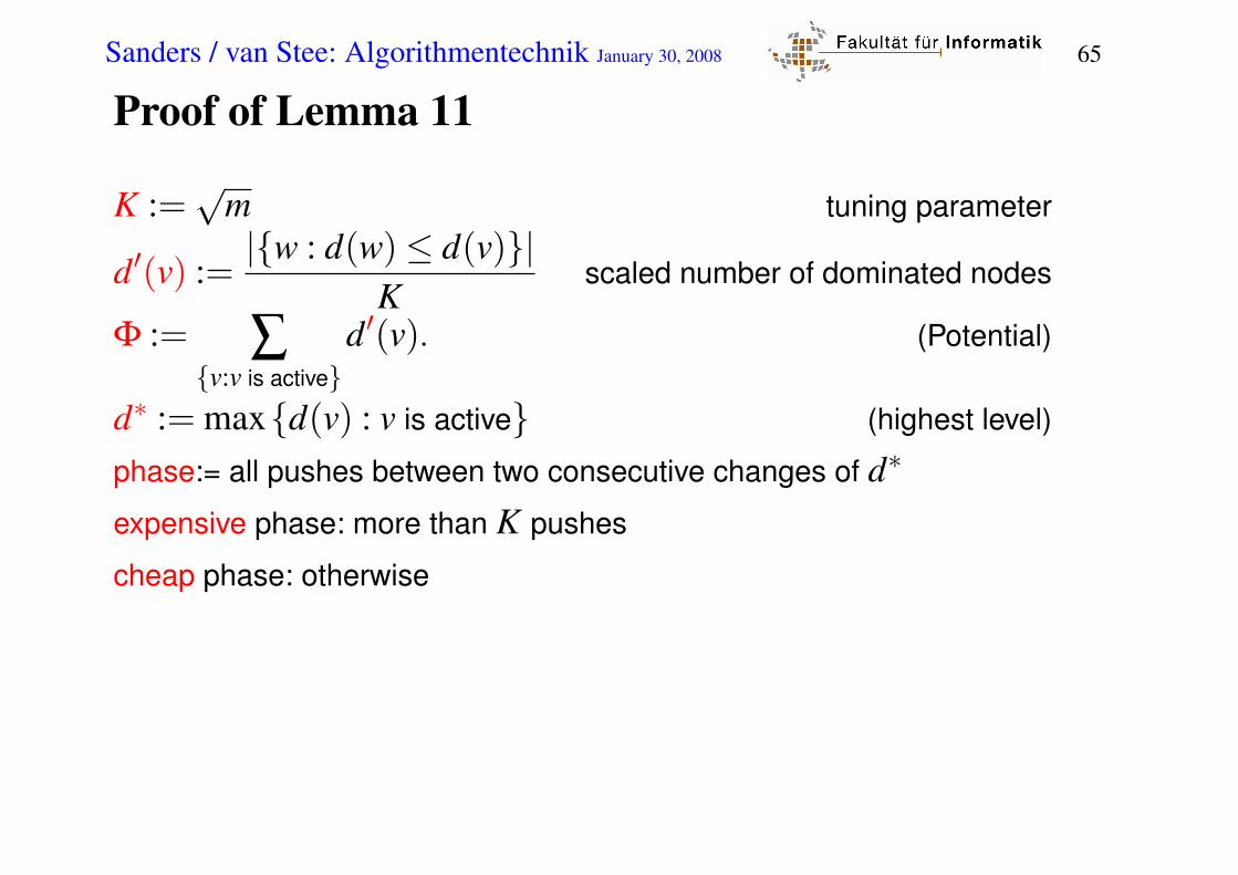
Proof of Lemma 11
K :=√
m tuning parameter
d′(v) :=|w : d(w)≤ d(v)|
Kscaled number of dominated nodes
Φ := ∑v:v is active
d′(v). (Potential)
d∗ := maxd(v) : v is active (highest level)
phase:= all pushes between two consecutive changes of d∗
expensive phase: more than K pushes
cheap phase: otherwise
Sanders / van Stee: Algorithmentechnik January 30, 2008 66
Claims:
1. ≤ 4n2K nonsaturating pushes in all cheap phases together
2. Φ≥ 0 always, Φ≤ n2/K initially (obvious)
3. a relabel or saturating push increases Φ by at most n/K.
4. a nonsaturating push does not increase Φ.
5. an expensive phase with Q≥ K nonsatu-
rating pushes decreases Φ by at least Q.
Lemma 6+Lemma 7+2.+3.+4.:⇒total possible decrease≤ (2n2 +nm) n
K + n2
K
Operation Amount
Relabel 2n2
Sat.push nm
This +5. :≤ 2n3+n2+mn2
K nonsaturating pushes in expensive phases
This +1. :≤ 2n3+n2+mn2
K +4n2K = O(n2√m
)nonsaturating
pushes overall for K =√
m ¤

Sanders / van Stee: Algorithmentechnik January 30, 2008 67
Claims:
1. ≤ 4n2K nonsaturating pushes in all cheap phases together
We first show that there are at most 4n2 phases
(changes of d∗ = maxd(v) : v is active).
d∗ = 0 initially, d∗ ≥ 0 always.
Only relabel operations increase d∗, i.e.,
≤ 2n2 increases by Lemma 6 and hence
≤ 2n2 decreases
——————————————————
≤ 4n2 changes overall
By definition of a cheap phase, it has at most K pushes.

Sanders / van Stee: Algorithmentechnik January 30, 2008 68
Claims:
1. ≤ 4n2K nonsaturating pushes in all cheap phases together
2. Φ≥ 0 always, Φ≤ n2/K initially (obvious)
3. a relabel or saturating push increases Φ by at most n/K.
Let v denote the relabeled or activated node.
d′(v) :=|w : d(w)≤ d(v)|
K≤ n
KA relabel of v can increase only the d′-value of v.
A saturating push on (u,w) may activate only w.

Sanders / van Stee: Algorithmentechnik January 30, 2008 69
Claims:
1. ≤ 4n2K nonsaturating pushes in all cheap phases together
2. Φ≥ 0 always, Φ≤ n2/K initially (obvious)
3. a relabel or saturating push increases Φ by at most n/K.
4. a nonsaturating push does not increase Φ.
v is deactivated (excess(v) is now 0)
w may be activated
but d′(w)≤ d′(v) (we do not push flow away from the sink)

Sanders / van Stee: Algorithmentechnik January 30, 2008 70
Claims:
1. ≤ 4n2K nonsaturating pushes in all cheap phases together
2. Φ≥ 0 always, Φ≤ n2/K initially (obvious)
3. a relabel or saturating push increases Φ by at most n/K.
4. a nonsaturating push does not increase Φ.
5. an expensive phase with Q≥ K nonsatu-
rating pushes decreases Φ by at least Q.
During a phase d∗ remains constant
Each nonsat. push decreases the number of nodes at level d∗
Hence, |w : d(w) = d∗| ≥ K during an expensive phase
Each nonsat. push across (v,w) decreases Φ by
≥ d′(v)−d′(w)≥ |w : d(w) = d∗|/K≥K/K = 1

Sanders / van Stee: Algorithmentechnik January 30, 2008 71
Claims:
1. ≤ 4n2K nonsaturating pushes in all cheap phases together
2. Φ≥ 0 always, Φ≤ n2/K initially (obvious)
3. a relabel or saturating push increases Φ by at most n/K.
4. a nonsaturating push does not increase Φ.
5. an expensive phase with Q≥ K nonsatu-
rating pushes decreases Φ by at least Q.
Lemma 6+Lemma 7+2.+3.+4.:⇒total possible decrease≤ (2n2 +nm) n
K + n2
K
Operation Amount
Relabel 2n2
Sat.push nm
This +5. :≤ 2n3+n2+mn2
K nonsaturating pushes in expensive phases
This +1. :≤ 2n3+n2+mn2
K +4n2K = O(n2√m
)nonsaturating
pushes overall for K =√
m ¤

Sanders / van Stee: Algorithmentechnik January 30, 2008 72
Heuristic Improvements
Naive algorithm has best case Ω(n2). Why? We can do better.
aggressive local relabeling:
d(v):= 1+min
d(w) : (v,w) ∈ G f
(like a sequence of relabels)
e=15
7
3
8
d=5
d=4
d=8
d=7
1
d=4
e=5
7
3
8
d=5
d=4
d=8
d=7
1
d=4
d=8

Sanders / van Stee: Algorithmentechnik January 30, 2008 73
Heuristic Improvements
Naive algorithm has best case Ω(n2). Why?
We can do better.
aggressive local relabeling: d(v):= 1+min
d(w) : (v,w) ∈ G f
(like a sequence of relabels)
global relabeling: (initially and every O(m) edge inspections):
d(v) := G f .reverseBFS(t) for nodes that can reach t in G f .
Special treatment of nodes with d(v)≥ n. (Returning flow is easy)
Gap Heuristics. No node can connect to t across an empty level:
if v : d(v) = i= /0 then foreach v with d(v) > i do d(v):= n

Sanders / van Stee: Algorithmentechnik January 30, 2008 74
Experimental results
We use four classes of graphs:
¤ Random: n nodes, 2n+m edges; all edges (s,v) and (v, t) exist
¤ Cherkassky and Goldberg (1997) (two graph classes)
¤ Ahuja, Magnanti, Orlin (1993)

Sanders / van Stee: Algorithmentechnik January 30, 2008 75
Timings: Random Graphs
Rule BASIC HL LRH GRH GAP LEDA
FF 5.84 6.02 4.75 0.07 0.07 —
33.32 33.88 26.63 0.16 0.17 —
HL 6.12 6.3 4.97 0.41 0.11 0.07
27.03 27.61 22.22 1.14 0.22 0.16
MF 5.36 5.51 4.57 0.06 0.07 —
26.35 27.16 23.65 0.19 0.16 —
n ∈ 1000,2000 ,m = 3nFF=FIFO node selection, HL=hightest level, MF=modified FIFO
HL= d(v)≥ n is special,
LRH=local relabeling heuristic, GRH=global relabeling heuristics

Sanders / van Stee: Algorithmentechnik January 30, 2008 76
Timings: CG1
Rule BASIC HL LRH GRH GAP LEDA
FF 3.46 3.62 2.87 0.9 1.01 —
15.44 16.08 12.63 3.64 4.07 —
HL 20.43 20.61 20.51 1.19 1.33 0.8
192.8 191.5 193.7 4.87 5.34 3.28
MF 3.01 3.16 2.3 0.89 1.01 —
12.22 12.91 9.52 3.65 4.12 —
n ∈ 1000,2000 ,m = 3nFF=FIFO node selection, HL=hightest level, MF=modified FIFO
HL= d(v)≥ n is special,
LRH=local relabeling heuristic, GRH=global relabeling heuristics

Sanders / van Stee: Algorithmentechnik January 30, 2008 77
Timings: CG2
Rule BASIC HL LRH GRH GAP LEDA
FF 50.06 47.12 37.58 1.76 1.96 —
239 222.4 177.1 7.18 8 —
HL 42.95 41.5 30.1 0.17 0.14 0.08
173.9 167.9 120.5 0.36 0.28 0.18
MF 45.34 42.73 37.6 0.94 1.07 —
198.2 186.8 165.7 4.11 4.55 —
n ∈ 1000,2000 ,m = 3nFF=FIFO node selection, HL=hightest level, MF=modified FIFO
HL= d(v)≥ n is special,
LRH=local relabeling heuristic, GRH=global relabeling heuristics
Sanders / van Stee: Algorithmentechnik January 30, 2008 78
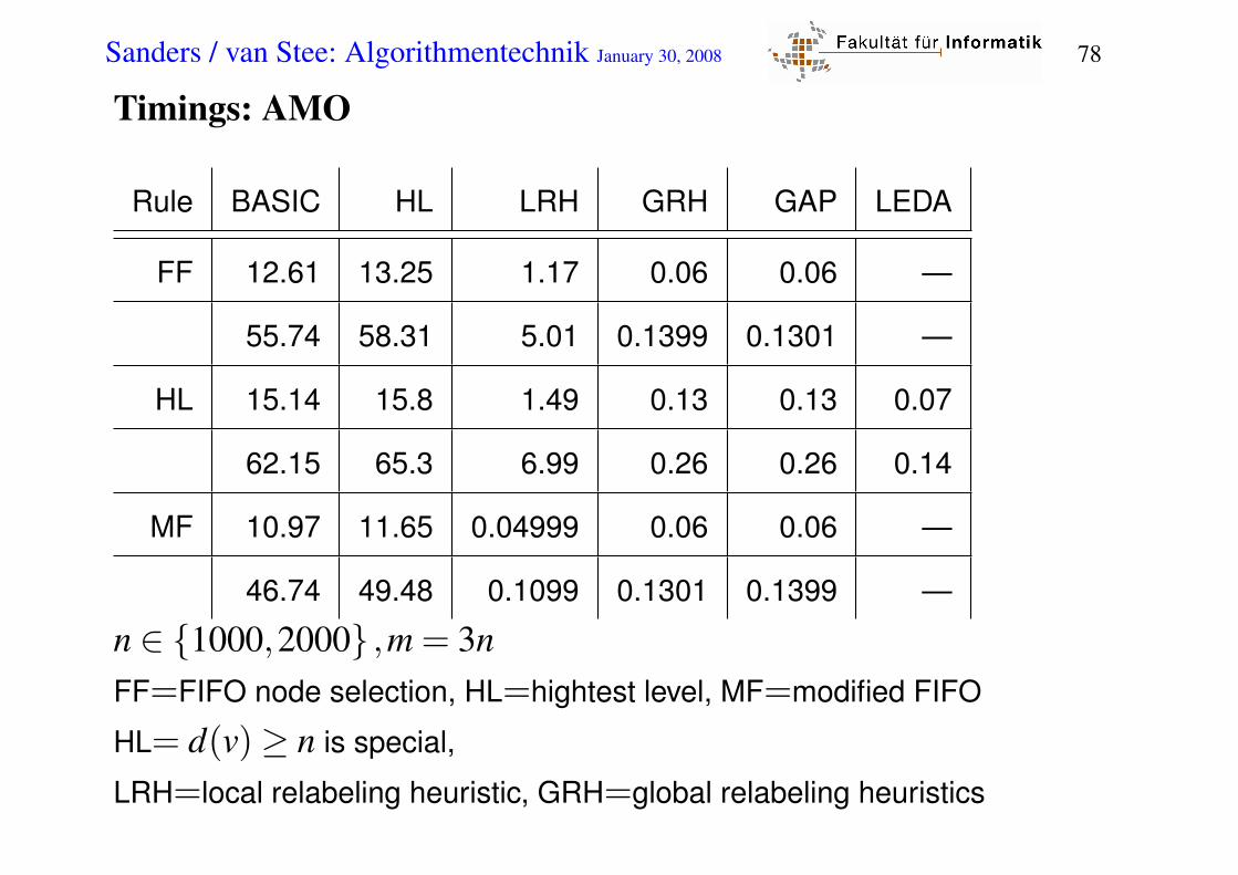
Timings: AMO
Rule BASIC HL LRH GRH GAP LEDA
FF 12.61 13.25 1.17 0.06 0.06 —
55.74 58.31 5.01 0.1399 0.1301 —
HL 15.14 15.8 1.49 0.13 0.13 0.07
62.15 65.3 6.99 0.26 0.26 0.14
MF 10.97 11.65 0.04999 0.06 0.06 —
46.74 49.48 0.1099 0.1301 0.1399 —
n ∈ 1000,2000 ,m = 3nFF=FIFO node selection, HL=hightest level, MF=modified FIFO
HL= d(v)≥ n is special,
LRH=local relabeling heuristic, GRH=global relabeling heuristics

Sanders / van Stee: Algorithmentechnik January 30, 2008 79
Asymptotics, n ∈ 5000,10000,20000
Gen Rule GRH GAP LEDA
rand FF 0.16 0.41 1.16 0.15 0.42 1.05 — — —
HL 1.47 4.67 18.81 0.23 0.57 1.38 0.16 0.45 1.09
MF 0.17 0.36 1.06 0.14 0.37 0.92 — — —
CG1 FF 3.6 16.06 69.3 3.62 16.97 71.29 — — —
HL 4.27 20.4 77.5 4.6 20.54 80.99 2.64 12.13 48.52
MF 3.55 15.97 68.45 3.66 16.5 70.23 — — —
CG2 FF 6.8 29.12 125.3 7.04 29.5 127.6 — — —
HL 0.33 0.65 1.36 0.26 0.52 1.05 0.15 0.3 0.63
MF 3.86 15.96 68.42 3.9 16.14 70.07 — — —
AMO FF 0.12 0.22 0.48 0.11 0.24 0.49 — — —
HL 0.25 0.48 0.99 0.24 0.48 0.99 0.12 0.24 0.52
MF 0.11 0.24 0.5 0.11 0.24 0.48 — — —

Sanders / van Stee: Algorithmentechnik January 30, 2008 80
Minimum Cost Flows
Define G = (V,E), f , excess, and cap as for maximum flows.
Let c : E → R denote the edge costs.
Consider supply : V →R with ∑v∈V supply(v) = 0. A negative supply
is called a demand.
Objective: minimize c( f ) := ∑e∈E
f (e)c(e)
subject to
∀v ∈V : excess(v) =−supply(v) flow conservation constraints
∀e ∈ E : f (e)≤ cap(e) capacity constraints

Sanders / van Stee: Algorithmentechnik January 30, 2008 81
The Cycle Canceling Algorithm for Min-CostFlow
Residual cost: Let e = (v,w) ∈ G f , e′ = (w,v).
c f (e) =−c(e′) if e′ ∈ E , f (e′) > 0, c f (e) = c(e) otherwise.
Lemma 13. A feasible flow is optimal iff6 ∃ cycle C ∈ G f : c f (C) < 0
Beweis. not here
A pseudopolynomial Algorithm:
f := any feasible flow// Exercise: solve this problem using maximum flowsinvariant f is feasible
while ∃ cycle C : c f (C) < 0 do augment flow around C

Sanders / van Stee: Algorithmentechnik January 30, 2008 82
Korollar 14 (Integrality Property:). If all edge capacities areintegral then there exists an integral minimum cost flow.

Sanders / van Stee: Algorithmentechnik January 30, 2008 83
Finding a Feasible Flow
set up a maximum flow network G∗ starting with the min cost flow
problem G:
¤ Add a vertex s
¤ ∀v ∈V with supply(v) > 0, add edge (s,v) with cap. supply(v)
¤ Add a vertex t
¤ ∀v ∈V with supply(v) < 0, add edge (v, t) with cap.−supply(v)
¤ find a maximum flow f in G∗
f saturates the edges leaving s⇒ f is feasible for Gotherwise there cannot be a feasible flow f ′ because f ′ could easily
be converted into a flow in G∗ with larger value.
Sanders / van Stee: Algorithmentechnik January 30, 2008 84
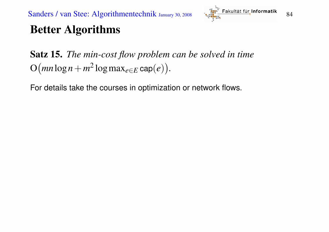
Better Algorithms
Satz 15. The min-cost flow problem can be solved in timeO
(mn logn+m2 logmaxe∈E cap(e)
).
For details take the courses in optimization or network flows.

Sanders / van Stee: Algorithmentechnik January 30, 2008 85
Special Cases of Min Cost Flows
Transportation Problem: ∀e ∈ E : cap(e) = ∞
Minimum Cost Bipartite Perfect Matching:
A transportation problem in a bipartite graph G = (A∪B,E ⊆ A×B)with
supply(v) = 1 for v ∈ A,
supply(v) =−1 for v ∈ B.
An integral flow defines a matching
Reminder: M ⊆ E is a matching if (V,M) has maximum degree one.
A rule of Thumb: If you have a combinatorial optimization problem. Try
to formulate it as a shortest path, flow, or matching problem. If this fails
its likely to be NP-hard.

Sanders / van Stee: Algorithmentechnik January 30, 2008 86
Maximum Weight Matching
Generalization of maximum cardinality matching. Find a matching
M∗ ⊆ E such that w(M∗) := ∑e∈M∗ w(e) is maximized
Applications: Graph partitioning, selecting communication partners. . .
Satz 16. A maximum weighted matching can be found in timeO
(nm+n2 logn
). [Gabow 1992]
Approximate Weighted Matching
Satz 17. There is an O(m) time algorithm that finds a matchingof weight at least maxmatchingM w(M)/2. [Drake Hougardy2002]
The algorithm is a 1/2-approximation algorithm.

Sanders / van Stee: Algorithmentechnik January 30, 2008 87
Approximate Weighted Matching AlgorithmM′:= /0invariant M′ is a set of simple pathswhile E 6= /0 do // find heavy simple paths
select any v ∈V with degree(v) > 0 // select a starting nodewhile degree(v) > 0 do // extend path greedily
(v,w):= heaviest edge leaving v // (*)M′:= M′∪(v,w)remove v from the graph
v:= wreturn any matching M ⊆M′ with w(M)≥ w(M′)/2//one path at a time, e.g., look at the two ways to take every other edge.

Sanders / van Stee: Algorithmentechnik January 30, 2008 88
Proof of Approximation Ratio
Let M∗ denote a maximum weight matching.
It suffices to show that w(M′)≥ w(M∗).
Assign each edge to that incident node that is deleted first.
All e∗ ∈M∗ are assigned to different nodes.
Consider any edge e∗ ∈M∗ and assume it is assigned to node v.
Since e∗ is assigned to v, it was available in line (*).Hence, there is an edge e ∈M01 assigned to v with w(e)≥ w(e∗).