sampling and indirect observations: a case-study of the
TRANSCRIPT

1
High-resolution species-distribution model based on systematic 1
sampling and indirect observations: a case-study of the wild ass in 2
the Negev Desert 3
4
Oded Nezer, Department of Environmental Engineering, Technion – Israel Institute of 5
Technology. [email protected] 6
Shirli Bar-David, Mitrani Department of Desert Ecology, Jacob Blaustein Institutes 7
for Desert Research, Ben Gurion University of the Negev. [email protected] 8
Tomer Gueta, Department of Environmental Engineering, Technion – Israel Institute 9
of Technology, Haifa 32000, Israel. [email protected] 10
Yohay Carmel*, Department of Environmental Engineering, Technion – Israel 11
Institute of Technology, Haifa 32000, Israel. [email protected]. Phone: 972-4- 12
8292609. 13
14
*Corresponding author. 15
16

2
Abstract 17
Species Distribution models (SDMs) are often limited by the use of coarse-resolution 18
environmental variables and by the number of observations needed to calibrate SDMs. 19
This is particularly true in the case of elusive animals. Here, we developed a SDM by 20
combining three elements: a database of explanatory variables, mapped at a fine 21
resolution; a systematic sampling scheme; and an intensive survey of indirect 22
observations. Using MaxEnt, we developed the SDM for the population of the Asiatic 23
wild ass (Equus hemionus), a rare and elusive species, at three spatial scales: 10, 100, 24
and 1000 m per pixel. We used indirect observations of feces mounds. We constructed 25
14 layers of explanatory variables, in five categories: water, topography, biotic 26
conditions, climatic variables and anthropogenic variables. Woody vegetation cover 27
and slopes were found to have the strongest effect on the wild ass distribution and 28
were included as the main predictors in the SDM. Model validation revealed that an 29
intensive survey of feces mounds and high-resolution predictor layers resulted in a 30
highly accurate and informative SDM. Fine-grain (10 m and 100 m) SDMs can be 31
utilized to: 1) characterize the variables influencing species distribution at high 32
resolution and local scale, including anthropogenic effects and geomorphologic 33
features; 2) detect potential population activity centers; 3) locate potential corridors of 34
movement and possible isolated habitat patches. Such information may be useful for 35
the conservation efforts of the Asiatic wild ass. This approach could be applied to 36
other elusive species, particularly large mammals. 37
Keywords: Equus hemionus; habitat preferences; Faeces; MAXENT; 38
SDM; spatially explicit model. 39
40

3
Introduction 41
Spatially explicit Species Distribution Models (SDMs) are commonly used for 42
purposes of conservation, environmental planning, and wildlife management 43
programs (Guisan et al. 2013). SDM models quantify the relationships between the 44
distribution and demography of a species and the environment (Peterson 2011). SDMs 45
allow us to study species distribution in large areas and even in remote habitats, where 46
logistic and financial restrictions preclude direct observations (Duff and Morrell 47
2007). They may be particularly useful for assessing the success of reintroduction 48
activities (Manel et al. 1999; Manel et al. 2001). Understanding habitat characteristics 49
and distribution determinants of reintroduced species is important in order to ensure 50
the protection of landscape components that are critical for the long-term persistence 51
of these species in the wild. 52
The use of environmental variables to explain and predict species distribution is not 53
trivial, since these relationships are complex, and a large number of variables are 54
involved (Guisan and Zimmermann 2000; Radosavljevic and Anderson 2014). It is 55
well known that the variables that affect the distribution of a species change with the 56
change of observation scale (Blank and Carmel 2012; Crawley and Harral 2001; Kent 57
et al. 2011; Stauffer and Best 1986). Coarse-scale distribution models may be 58
preferred in, for example, bio-geographic studies. In contrast, fine-scale distribution 59
models can depict local scale phenomena such as essential corridors and animal 60
passages and effects of roads and rivers, which coarse-scale models cannot detect. 61
Thus, fine-scale distribution models may be preferable for conservation planning and 62
management (Hess et al. 2006). Yet, in most studies, the selection of resolution is a 63
consequence of the availability and quality of data pertaining to the specific study 64
area, which is typically the limiting factor in distribution studies (Elith et al. 2006; 65

4
Hess et al. 2006). Data layers used in such studies are typically derived from global 66
databases where 1 km2 is considered the finest resolution. 67
Presence/absence information is thought to be preferred to presence-only information 68
in SDMs. However, presence/absence information is more difficult or impossible to 69
obtain than Presence-only information (Kent et al. 2011; Pearce and Boyce 2006; 70
Tsoar et al. 2007). However, presence-only data may be subject to large errors due to 71
small sample size and biased samples (Graham et al. 2004; Phillips and Elith 2013). A 72
systematic data-collection survey, designed to collect data at precise locations should 73
largely reduce these biases. 74
Indirect observations, and in particular dung surveys, are common non-invasive 75
approaches for obtaining information about the presence of species and habitat 76
selection. They are particularly useful when the studied species is hard to find due to 77
its elusive behavior, rarity, or habitat (Fernandez et al. 2006; Vina et al. 2010). The 78
use of indirect observations in SDMs requires a clear connection between the 79
presence of the species and the feces (Gallant et al. 2007; Kays et al. 2008; Perinchery 80
et al. 2011). Systematic dung survey, conducted in sites selected to represent the 81
entire range of environmental conditions in a region, can be an appropriate solution to 82
sampling-bias problems (Fernandez et al. 2006; Norris 2014; Vina et al. 2010). 83
Here, we developed a species distribution model for the population of the Asiatic 84
Wild Ass (Equus hemionus), a rare and elusive species that was reintroduced into the 85
Negev Desert in Israel. We combined three elements in order to overcome the 86
obstacles in developing SDMs: a database of spatial layers of explanatory variables, 87
mapped at a very fine resolution; a systematic sampling scheme; and an intensive 88
survey of indirect observations, presence of feces mounds. This approach led to 89
important insights regarding the habitat preferences of this species. 90

5
Methods 91
Study species 92
The Asiatic wild ass is an endangered species (Moehlman et al. 2008). In the past, the 93
Syrian wild ass (E. h. hemippus) subspecies was found in the Middle East, and 94
became extinct in the wild at the beginning of the 20th century (Groves 1986; Saltz et 95
al. 2000; Schulz and Kaiser 2013). In 1968, a breeding core was established in Israel 96
using individuals from the subspecies E.h. onager and E. h. kulan brought from Iran 97
and Turkmenistan, respectively. In 1982 the Israel Nature and Parks Authority 98
initiated a reintroduction program of the Asiatic wild ass (from the breeding core of 99
these two subspecies (Saltz et al. 2000). The first individuals were released near Ein- 100
Saharonim in Makhtesh Ramon (Fig. 1). By 1993, three additional releases were 101
conducted at this site and two more in the Paran streambed (Saltz and Rubenstein 102
1995). A total of 38 individuals were released. The wild ass population expanded its 103
range in the Negev Desert and the Arava valley (Saltz and Rubenstein 1995), and the 104
current population is estimated at more than 250 individuals (Renan et al. 2015). 105
Study area 106
The study area extends over approximately 3,000 km2 in the central part of the Negev 107
Desert (Fig. 1). The area is arid and characterized by high daytime temperatures (on 108
average 33°C) and relatively low night-time temperatures (on average 12°C). Mean 109
annual precipitation ranges between 30 mm and 150 mm (Stern et al. 1986). Elevation 110
ranges between 50-1033 m, and the area has a complex geomorphological structure. 111
The bedrock is mainly hard limestone, resulting in a cliffy landscape and leveled 112
floodplains. The majority of the area is drained by two main ephemeral streambeds 113
(wadis) – Nekarot and Paran. There are several latitudinal geological faults in the 114

6
region that create a steep terraced landscape. Flash floods are a common phenomenon 115
after rain events. The flash floods fill water holes in the streambeds, which may hold 116
for a few months. There are very few natural water sources that provide water year- 117
round. Vegetation is mostly limited to streams and their surroundings and generally 118
located on the banks. Vegetation in the streams is mostly of a Saharo-Arabian origin, 119
with a Sudanian component in the Arava (Danin 1999). It is dominated by three native 120
Acacia tree species, Acacia raddiana, A. tortilis, and A. pachyceras. 121

7
122
Figure 1. The study region, reintroduction and sampling sites in the Negev Desert, 123
Israel. 124
125
Data collection 126
We selected 122 sampling sites using an approximate systematic sampling scheme 127
(Fig. 1) in order to capture the full range of conditions found in the study region. To 128

8
ensure accurate representation of the environmental conditions in the sampling sites, 129
we stratified the sampling locations according to three environmental parameters: 130
distance from permanent water sources, altitude, and mean temperature of the hottest 131
month. Based on our prior knowledge of the study species and a literature review 132
(Henley and Ward 2006; Henley et al. 2007; Saltz and Rubenstein 1995; Saltz et al. 133
1999), we considered these environmental variables to have a high potential for 134
explaining wild ass distribution. These variables were represented by GIS layers and 135
combined into a three banded composite, on which we performed K-means 136
unsupervised classification using ERDAS IMAGINE V 9.1. The objective of this 137
classification was to divide the study region into polygons with similar combinations 138
of these variables (Carmel and Stoller-Cavari 2006). The 122 sampling sites were 139
systematically distributed among these polygons. 140
In each sampling site we conducted a feces survey. Fecal droppings of wild ass 141
constitute a straightforward indicator for species presence because they are deposited 142
frequently, and remain visible in the desert environment for several months (up to 143
about a year). The survey in each site was composed of three 500 m belt transects 144
arranged as an equilateral triangle with a total length of 1500 m, and divided into 150 145
survey units of 10X10 m per site. One of the triangle sides was always laid on a dry 146
river-bed nearest to the point defined as the center of the sampling site. We recorded 147
observations at a distance of 5 m on either side of the transect, where detection 148
probability of feces was 100%. The exact location of feces mound (droppings as well 149
as dung piles) observed on the transect were recorded using a GPS at a spatial 150
accuracy of 4 m. The number of feces mounds within each 10 m pixel was recorded. 151
During January 2009 to June 2009 we surveyed 122 sites and explored 150 units per 152

9
site, with a total sampled area of 183 ha. For the ‘presence-only’ SDM, we classified 153
each unit as ‘present’ if one or more feces mounds were found in that unit. 154
Data analysis 155
Explanatory variables 156
We devoted extensive efforts to create a high resolution digital data set of 157
environmental variables. We generated 14 spatial layers (Table 1), from which the 158
model predictors were derived. These layers pertain to five main categories (Table 1): 159
vegetation (one variable), topography (4), climate (2), anthropogenic variables (5), 160
and distance from water (2 variables). The vegetation layer was derived from a 161
complex processing of an aerial photo (Appendix 1). Topography was derived from a 162
DEM of the area, at an original resolution of 10 m. Climate layers had an original 163
resolution of 1 km, and were up-scaled to a 10 m resolution. Distance to—layers were 164
constructed using Euclidean distance to specific elements on the map at an original 165
resolution of 10 m. In order to reduce multicollinearity, correlation coefficients were 166
calculated between each pair of variables; in pairs with a high correlation (>0.65 or <- 167
0.65, Pearson correlation), one of the variables was eliminated from the model. A map 168
of each explanatory variable appears in Appendix 2. 169
Table 1. Predictors used in the distribution model of wild ass. Stars (*) indicate 170
variables eliminated from the model due to high correlation with other variables. 171
# Category Description Retrieval information
1 Vegetation
Percentage of woody vegetation
cover (shrubs and trees with a
radius greater than 0.2m). Each 10
m cell represents an averaged
vegetation cover over a 100m
radius.
Manual digitization from
orthophoto.
2
Topography
Altitude above sea level
Generated from contour dataset
retrieved from Survey of Israel
(MAPI)
3 Slope (between 0-90 degrees) Generated from Altitude using
ArcMap 10

10
4 Aspect (between 0-360 degrees) Generated from Altitude using
ArcMap 10
5 Cumulative drainage Generated from slope using
ArcMap 10
6 Climate
*Mean annual precipitation Retrieved from the GIS Lab at
the Hebrew University of
Jerusalem 7 *Mean temperature in August
8
Anthropogenic
factors
*Distance from roads Generated in ArcMap 10
9 *Distance from reintroduction sites Generated in ArcMap 10
10 Distance from military bases and
settlements Generated in ArcMap 10
11 Military training sites (binary) Manual digitization from
orthophoto.
12 Nature reserve (binary) Manual digitization from
orthophoto.
13 Water
Distance from all permanent water
sources including springs and
leaking pipes
Generated in ArcMap 10
14 *Distance from watering holes Generated in ArcMap 10
172
Statistical model 173
We used the “Maximum Entropy” model MAXENT V3.3.1 (Kumar et al. 2009; 174
Phillips et al. 2006; Phillips and Dudik 2008). We selected this model out of a large 175
number of possible models, since it was ranked in several comparative studies as one 176
of the most effective models for predicting species distribution on the basis of 177
presence-only data (Elith et al. 2006; Elith et al. 2011; Jeschke and Strayer 2008; 178
Phillips et al. 2006; Radosavljevic and Anderson 2014). The MAXENT algorithm 179
operates on a set of constraints that describes what is known from the sample of the 180
target distribution (i.e., the presence data). Maxent characterizes the background 181
environment with a set of background points from the study region. However, unlike 182
the case of presence–absence data, the species occurrence at these background points 183
is unknown. MAXENT predicts the probability distribution across all cells in the 184
study area based on the presence data and, to prevent over-fitting, employs maximum 185
11
entropy principles and regularization parameters (Phillips et al. 2006). MAXENT 186
produces two outputs: a probabilistic distribution map describing the establishment 187
probability of the species in a specific site and the relative weight of each explanatory 188
variable. Distribution maps of the Asiatic wild ass were obtained by applying 189
MAXENT models to all cells in the study region, using a logistic link function to 190
yield a habitat suitability index between zero and one (Phillips and Dudik 2008). We 191
ran the model in three spatial resolutions: 10 m, 100 m and 1 km, with 106, 105 and 192
104 background points respectively. Recommended values were used for the 193
convergence threshold (10-5), maximum number of iterations (500), and regularization 194
multiplier (1). Response functions were constrained to only three feature types: 195
Linear, Threshold and Hinge. 196
In order to estimate the percent contribution of each environmental variable, in each 197
iteration of the training algorithm, the increase in Regularized gain is added to the 198
contribution of the corresponding variable. In order to estimate the permutation 199
importance of each environmental variable, in turn the values of the corresponding 200
variable on training presence and background data are randomly permuted. The model 201
is reevaluated on the permuted data, and the resulting drop in Training AUC is 202
normalized to percentages. In order to estimate if occurrence data of the wild ass are 203
spatially autocorrelated, we calculated Moran's I Index (Moran 1950) for each spatial 204
resolution separately (10 m, 100 m and 1 km). 205
Model validation 206
We validated the model using: 1) MAXENT's five performance measures and 2) a 207
cross-validation procedure. MAXENT model generates three gain measures and two 208
AUC measures. Gain measures the goodness of fit of a models, it represents the 209
likelihood of presence records compared to background records (Phillips 2005). A 210

12
gain of 1.6 means that an average presence location has a relative probability of e1.6, 211
which is five times higher than an average background point. Regularized training 212
gain accounts for the number of predictors in the model to address overfitting; 213
Unregularized training gain has no compensation for the number of predictors in the 214
model; and Test gain is calculated from presence records held out to test the model. 215
AUC is the area under the curve of the receiver operating characteristic (ROC) plot. 216
ROC curves are widely used for validating SDMs and for comparing between models 217
(Elith et al. 2006; Hernandez et al. 2006; Marmion et al. 2009). The AUC values 218
range between 0 and 1, where 1 represents perfect prediction ability of the model and 219
0.5 represents prediction that is no better than random. Training AUC calculates AUC 220
using the training data; and Test AUC calculates AUC using the test data. A cross- 221
validation procedure was used to estimate errors around predictive performance on 222
held-out data (Elith et al. 2011). Occurrence data are randomly split into a number of 223
equal-size groups (folds), and models are created leaving out each fold in turn. The 224
left-out folds are then used for evaluation. Cross-validation uses all of the data for 225
validation. A 10-folds cross-validation procedure was used for the 10 m and 100 m 226
models, and a 5-folds cross-validation procedure was used for the 1 km model. 227
Results 228
We recorded a total of 3,232 feces mounds in 18,300 survey units (10 m cells). Feces 229
mounds were found in 115 of the 122 sampling sites. The number of mounds per site 230
ranged from 0 to 124. Five potential explanatory variables were eliminated from the 231
model (Table 1) due to high correlation coefficient (>0.65 or <-0.65, Pearson 232
correlation, see Appendix 3), leaving nine variables in the model. Three of these 233
spatial data layers, namely vegetation, slope, and altitude, were considered as the most 234

13
influential explanatory variables by the MAXENT algorithm, accounting together for 235
~85% of the cumulative relative contribution (Table 2). Woody vegetation density 236
was found to have the strongest effect on the Asiatic wild ass distribution (Table 2; 237
Appendix 4). The response curve of woody vegetation cover (Appendix 5) showed an 238
increasing presence of the animals with increasing vegetation cover, leveling off 239
sharply at the saturation point (>72% coverage). Slope was the second most important 240
variable (Table 2) and was inversely related to wild ass distribution (Appendix 5). In 241
slopes steeper than 20°, no feces mounds were found. Altitude was the third most 242
important variable, with 12% relative contribution. The other six explanatory 243
variables that were included in the model had a lower effect on the distribution of wild 244
ass, together accounting for ~15% of the relative contribution to the model, Table 2. 245
The performance of the three models (10 m, 100, and 1 km) differed markedly. 246
The 10 m model yielded the highest averaged values in all five performance measures 247
(Table 3), indicating high predictive capacity. The 1 km model yielded the lowest 248
values in all measures, with extremely low values for Test gain (-0.02) and Test AUC 249
(0.67), suggesting poor predictive capacity at this scale. The cross-validation 250
procedure revealed high consistency between the different runs, since standard 251
deviation values were relatively low (Table 2 and 3). 252
Table 2. Percent contribution and permutation importance of the predictor variables 253
for the 10 m resolution MAXENT model for wild ass. See Statistical model section in 254
the Methods for an explanation. Standard deviation is shown in parentheses. 255
Explanatory variable
Relative
contribution in %
(± Std)
Permutation
importance in %
(± Std)
Vegetation 54.5 (0.44) 47.83 (0.93)
Slope 18.04 (0.41) 28.83 (1.31)
Altitude (DEM) 11.97 (0.41) 9.45 (0.73)

14
Distance from all permanent and temporary
water sources 6.76 (0.26) 6.44 (0.32)
Distance from military bases and settlements 5 (0.21) 4.43 (0.36)
Cumulative drainage 1.66 (0.14) 1.24 (0.15)
Nature reserve 1.39 (0.13) 0.95 (0.18)
Aspect 0.36 (0.07) 0.49 (0.08)
Military training sites 0.33 (0.06) 0.33 (0.09)
256
Table 3. The averaged MAXENT performance measures calculated using a 10-folds 257
or a 5-folds cross-validation procedure. Standard deviation is shown in parentheses. 258
Models
Model performance measures: 10 m model 100 m model 1 km model
Regularized training gain 1.63 (0.01) 1.16 (0.01) 0.64 (0.03)
Unregularized training gain 1.94 (0.01) 1.43 (0.01) 0.97 (0.04)
Test gain 1.82 (0.06) 1.26 (0.12) -0.02 (0.07)
Training AUC 0.93 (0) 0.9 (0) 0.85 (0.01)
Test AUC 0.92 (0.01) 0.88 (0.01) 0.67 (0.02)
259
Occurrence data at a 10 m resolution had a relatively low spatial autocorrelation 260
(Moran's I Index of 0.13), while the 100 m and 1 km resolutions had higher values 261
(0.38 and 0.22 respectively). 262
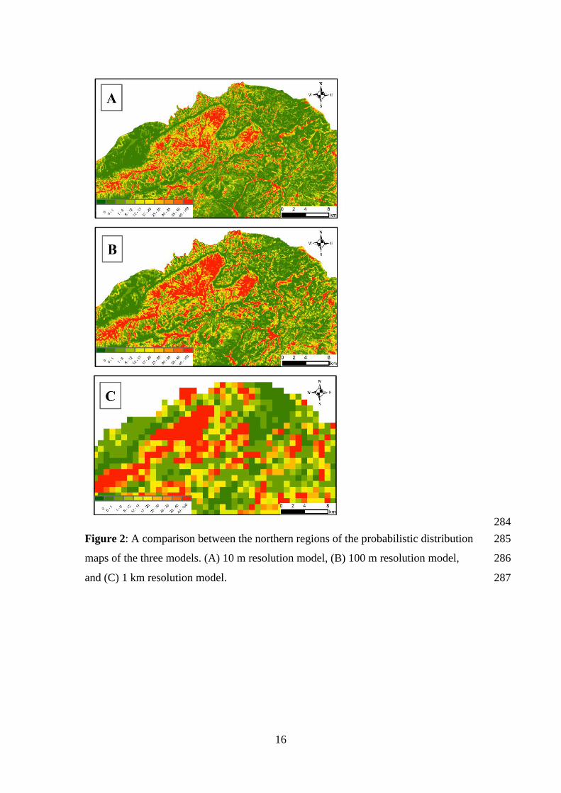
The probabilistic distribution map was heterogeneous and informative at the very 263
fine scale of 10 m, and the fine scale of 100 m (Fig. 2A-B), and much less informative 264
at the scale of 1 km (Fig. 2C). The strong effect of streambeds on the species 265
distribution was apparent at the two finer scales: areas of high probability of presence 266
were in streambeds (wadis) characterized by woody vegetation and moderate terrain. 267
The high resolution allowed detection of the following trends and phenomena at: [1] 268
Possible convenient movement corridors in a matrix of unsuitable environment, which 269
15
enable landscape connectivity among sites (Fig. 4A). [2] Isolated local sites/areas of 270
high suitability for the wild ass (high-quality habitat "islands") situated within broad 271
areas of low quality habitat (Fig. 4B). [3]. Human-induced local entities that affect the 272
distribution, e.g., the influence of roads on the quality of proximate habitats (Fig. 4C, 273
see discussion for details). [4] Important geomorphologic features that affect the 274
distribution, e.g., streambeds (Fig. 4D). 275
In contrast to the high variability visualized at fine scale, this map did not show 276
regional trends or gradients at the scale of the study area. Sites with very high and 277
very low probabilities of wild ass presence were found near each other throughout the 278
entire study area; however, in several areas, a spatial continuity of high value sites 279
was noticeable: Makhtesh Ramon (A), Paran streambed (B), the upper part of Nekarot 280
streambed (C), and the Lotz potholes (Borot Lotz) (D) (Fig. 3). These areas have the 281
potential to serve as activity centers for the population. A spatial continuum of sites 282
with low suitability for the Asiatic wild ass also was discernable (Fig. 3, points E-H). 283
16
284
Figure 2: A comparison between the northern regions of the probabilistic distribution 285
maps of the three models. (A) 10 m resolution model, (B) 100 m resolution model, 286
and (C) 1 km resolution model. 287

17
288
Figure 3: Probabilistic distribution maps of a 10 m resolution model for the Asiatic 289
wild ass in the Negev. Potential wild ass activity centers: Makhtesh Ramon (A), Paran 290
streambed (B), the upper part of Nekarot streambed (C) and the Lotz potholes (Borot 291
Lotz) (D). A spatial continuum of sites with low suitability: the Paran Stream Estuary 292
(E), the region south of Mount Karkom (F), Be’er Menuha (G), and the Eastern part 293
of Makhtesh Ramon (H). Stars indicate reintroduction sites. 294
295

18
296
Figure 4. Detecting landscape features on the high-resolution map: (a) Potential 297
movement corridors, (b) Isolated habitat patches, (c) Important geomorphologic 298
features, (d) Anthropogenic effects on habitat quality (roads effect increased roadside 299
vegetation). Colors represent predicted habitat suitability: from green, low suitability, 300
to red, high suitability. 301

19
Discussion 302
In this study we combined three elements in order to develop a predictive distribution 303
model for the wild ass, a rare and elusive animal: a database of spatial layers of 304
explanatory variables, mapped at a very fine resolution; a systematic sampling 305
scheme; and an intensive feces mound survey. The results indicate that this approach 306
yields an accurate and informative model. 307
Factors affecting wild ass distribution 308
The most important variable in the model was the percentage of woody vegetation 309
cover. Its relative contribution (54.5%) was much higher than that of the other 310
variables. The importance of vegetation to the wild ass distribution is consistent with 311
previous studies (Davidson et al. 2013; Giotto et al. 2015; Henley et al. 2007). The 312
strong vegetation effect on the distribution is a result of its nutritional value (St-Louis 313
and Côté 2014), the partial shade it offers, its value for hiding, and in arid areas the 314
vegetation is a favorable microhabitat with reduced temperatures (Belsky et al. 1993). 315
The second most important variable in the model was slope (relative contribution 316
of 18.04%). The Asiatic wild ass prefers moderate over steep terrain, and avoids steep 317
slopes. This observation was supported by previous studies (Davidson et al. 2013; 318
Giotto et al. 2015; Henley et al. 2007). The next variables in order of importance were 319
altitude (11.97%) and distance from water sources (6.76%). The positive effect of 320
altitude on wild ass distribution is probably related to lower temperatures associated 321
with higher elevations. The Negev is a hyper- arid desert and we expected that 322
distance from water sources would be a major predictor of wild ass distribution. 323
Indeed, the water sources themselves were found to be centers of wild ass activity. 324
However, the daily movement range of the wild ass can reach up to twenty km in each 325

20
direction (Saltz et al. 2000), and feces are distributed across most of the study area. 326
This may explain why the distance from water source was not a major determinant of 327
wild ass distribution. 328
Resolution 329
Model performance 330
Constructing models at various spatial resolutions and comparing between them 331
enabled us to quantify the effect of resolution on SDM performance. Seemingly, 332
model performance increased with increasing model resolution (Table 3). This finding 333
contradicts a previous study (Guisan et al. 2007) of the effect of degrading model 334
resolution on the performance of SDMs, who found that using finer cell sizes (from 1 335
km to 100 m, and from 10 km to 1 km) does not have a major effect on model 336
predictions. Yet, our results suggest that when the effective resolution of the 337
predictors was 10 m (102 m2), the model provides useful insights regarding the species 338
distribution that are not possible at coarser scales, as is elaborated in the following 339
section. 340
AUC is one of the most commonly used statistics to characterize model 341
performance (Yackulic et al. 2013), but its usage has been strongly criticized, 342
particularly with presence-only data (Gueta and Carmel 2016; Jiménez‐Valverde et al. 343
2013; Lobo et al. 2008; Yackulic et al. 2013), since it ignores the predicted probability 344
values and the goodness-of-fit of the model (Yackulic et al. 2013). Corroborating 345
these views, our 1 km model had a high Training AUC value (0.85) whereas the Test 346
gain showed near zero predictive capability (Table 3). This reveals AUC's low 347
informative value and its inadequacy as a performance index in presence-only 348
modelling framework. Gain indices are more sensitive indicators of model 349
performance (Gueta and Carmel 2016). 350

21
High-resolution spatial layers of explanatory variables 351
We invested considerable resources and effort to produce and obtain the layers of 352
explanatory variables at a spatial resolution of 10 m wherever possible. For climatic 353
variables, the original spatial resolution is 1 km. In contrast, the original resolution of 354
the vegetation and topography layers was 10 m. Indeed, these two variables were the 355
most important predictors in the 10 m model, somewhat less so in the 100 m model, 356
and nearly meaningless in the 1 km model. 357
Distribution models of large mammals with large home ranges are typically 358
constructed at resolutions of 100 – 10,000 m (e.g., (Bellamy et al. 2013), 2-6 orders of 359
magnitude lower than the 10 m resolution of the present study. Apparently, the two 360
predictors found to be the most important, vegetation and slope, appeared nearly 361
meaningless at a resolution of 1000 m. The distribution map constructed at this coarse 362
scale was not very informative. 363
High-resolution distribution map 364
The distribution map obtained by the model enabled us to examine the relative habitat 365
suitability of each site for the wild ass at a fine resolution. The fine-grain image in 366
Fig. 3 illustrates that low quality habitats are found within broad areas of suitable 367
habitat, and vice versa. The high resolution of the map allowed the detection of four 368
habitat components as important for the species’ use of space (Fig. 4): (a) Potential 369
movement corridors (Fig. 4A). Connectivity within the species’ range is essential for 370
the spatial, demographic and genetic dynamics of animal populations and their 371
persistence over time (Colbert et al. 2001; Saccheri et al. 1998) and should be 372
recognized as a high conservation priority (Beier et al. 2006). Identifying connectivity 373
corridors is highly important for the protection of the species, since they may facilitate 374
wild ass movements within a matrix of less suitable areas, enabling connectivity 375

22
between high-quality habitats (Fig. 2, points A-D). (b) Isolated habitat patches (Fig. 376
4B). Isolated sites or small fragments of high habitat quality within low quality areas 377
may constitute potential ‘stepping stones’ sites that aid in connecting between activity 378
centers. (c) Important geomorphologic features (Fig. 4C). The high-resolution map 379
indicated clearly the importance of streambeds, including first order streams, in the 380
distribution patterns of the wild ass. In coarser maps, the influence of the streambeds 381
cannot be detected. (d) Anthropogenic effect on distribution. Anthropogenic features 382
may influence distribution patterns of species and therefore it is important that they be 383
identified (Valverde et al. 2008). For example, based on the high-resolution wild ass 384
distribution model, roads were found to increase considerably the quality of habitats 385
in the proximate areas of the roads (Fig. 4D). However, in a specific case, the road 386
effect led to high density of roadside vegetation. The high vegetation quality, in turn, 387
attracted wild asses to the proximity of the road, and several road-kills of wild asses 388
were reported in this area, calling for roadside vegetation management (Asaf Tsoar, 389
personal communication). This example illustrates the importance of the model as a 390
tool to identify such potential negative anthropogenic effects. 391
Sampling 392
Systematic sampling of presence data 393
Many distribution models that are based on presence-only data suffer from 394
inaccuracies, due to biased sampling (e.g., multiple observations near roads and 395
accessible sites) and a distribution of observations that is unrepresentative of the range 396
of environmental conditions in the study region (Barry and Elith 2006; Elith et al. 397
2011; Kramer-Schadt et al. 2013; Phillips and Elith 2013). In this study, we 398
implemented an approximate systematic sampling scheme based on the spatial pattern 399
of major environmental conditions in the study region, thus reducing the 400

23
aforementioned errors. A common problem in sampling rare species is a zero-inflated 401
distribution of records. In order to reduce this problem, dry river beds were over- 402
represented based on a prior knowledge that wild asses are usually found within 403
riverbeds. Still, two-thirds of the samples were located off riverbeds. However, due to 404
the dense network of riverbeds and the high density of sampling sites – only few areas 405
were out of the reach of this sampling scheme (Fig. 1), and the possible bias was 406
minimal. 407
Indirect observations for presence data 408
Predictive distribution models are usually based on direct observations. Creating a 409
database of direct observations of an elusive organism with a small population, in a 410
region with very limited accessibility is a very complicated task (Lozano et al. 2003; 411
Sharp et al. 2001). Therefore, it was proposed that indirect observations (tracks, feces) 412
may replace direct observations, when there is a clear connection between the 413
presence of the species and the indirect observations (Fernandez et al. 2006; Kays et 414
al. 2008; Perinchery et al. 2011; Vina et al. 2010). In this study, we relied on indirect 415
observations using feces mounds as the basis for presence data. The major advantage 416
of surveying feces mounds is that they remain in the field after the animal leaves, 417
increasing the probability of recording activity in sites visited by the species. These 418
factors are enhanced in a desert environment, since in arid regions the decomposition 419
rate of the feces is slower, and mounds may last for long periods, in the case of the 420
wild asses in the Negev up to a year. The large number of observations is a major 421
component of the strength and reliability of a distribution model (Barry and Elith 422
2006).The feces surveys in our study led to a large number of observations. Obtaining 423
a similar sized database using direct observations would have required a much greater, 424
longer and costlier sampling effort. 425

24
Implications for conservation 426
SDMs can help to design conservation policies (Guisan and Zimmermann 2000). The 427
endangered Asiatic wild ass can become a focus of conservation interest due to its 428
impressive appearance, rarity, reintroduction process and its pivotal function in the 429
Negev ecosystem (Polak et al. 2014). The SDM constructed in this study can serve to 430
locate favorable high-quality patches, and potential future expansion directions of the 431
species in the Negev Desert. It can also be used to locate potential routes and 432
corridors among activity centers which are important to maintain connectivity within 433
the population. Model predictions can then be validated by conducting field surveys 434
(Davidson et al. 2013). This information can serve as the basis for developing 435
conservation and management strategies for the wild ass. Specifically, the map 436
enabled us to identify large continuous geographic areas of suitable habitat, which 437
constitute potential activity centers. Three of the continuous areas identified in the 438
map (central Makhtesh Ramon, Paran streambed, and Borot Lotz; Fig. 3) were 439
confirmed in the field as significant activity centers, based on direct observations. 440
Two of these sites – the Paran streambed and the central part of Makhtesh Ramon 441
overlap with the reintroduction sites. However, distance from the reintroduction sites 442
was not found to be a significant factor affecting species distribution in the statistical 443
model. Each one of the three activity centers contains a permanent water source. The 444
model further enabled us, in a parallel study, to identify areas with low landscape 445
connectivity among activity centers (Gueta et al. 2014). These areas were suggested to 446
limit gene flow, leading to the relative isolation of a subpopulation and to the 447
development of population genetic structure in the reintroduced wild ass population 448
(Gueta et al. 2014). Limited gene flow among activity centers may further affect the 449

25
population genetic diversity (Renan et al. 2015) which is essential for the population's 450
long-term viability (Hughes et al. 2008). 451
The distribution model can also be used to locate a potential direction for 452
expanding the wild ass range, by projecting the model onto additional areas (Bar- 453
David et al. 2008). It is important to identify areas of potential spatial expansion, in 454
order to ensure the protection and maintenance of landscape connectivity, which is 455
essential for the species’ distribution and, hence, for its persistence in the wild. 456
457
Acknowledgement 458
We would like to thank David Saltz, Alan R. Templeton, and Amos Bouskila for their 459
contributions to this study; Itamar Giladi for providing insightful comments that 460
greatly improved the manuscript. This research was supported by the United States- 461
Israel Binational Science Foundation Grant 2011384 awarded to S. B-D, A. R. 462
Templeton and A. Bouskila. GIS layers were provided by the GIS Department of the 463
Israel Nature and Parks Authority. This is publication <xxx> of the Mitrani 464
Department of Desert Ecology. 465
466

26
References 467
Bar-David S, Saltz D, Dayan T (2005) Predicting the spatial dynamics of a 468
reintroduced population: the Persian fallow deer Ecological Applications 469
15:1833-1846 470
Bar-David S, Saltz D, Dayan T, Shkedy Y (2008) Using spatially expanding 471
populations as a tool for evaluating landscape planning: The reintroduced 472
persian fallow deer as a case study Journal for Nature Conservation 16 164 473
Barry S, Elith J (2006) Error and uncertainty in habitat models Journal of Applied 474
Ecology 43:413-423 475
Beier P, Penrod K, Luke C, Spencer W, Cabañero C (2006) South coast missing 476
linkages: Restoring connectivity to wildlands in the largest metropolitan area 477
in the united states. In: Crooks KR, Sanjayan M (eds) Connectivity 478
Conservation. Cambridge University Press, Cambridge, United Kingdom, pp 479
555-586 480
Bellamy C, Scott C, Altringham J (2013) Multiscale presence-only habitat suitability 481
models: fine-resolution maps for eight bat species Journal of Applied Ecology 482
50:892-901 483
Belsky A, Mwonga S, Amundson R, Duxbury J, Ali A (1993) Comparative effects of 484
isolated trees on their undercanopy environments in high- and low-rainfall 485
savannas Journal of Applied Ecology 30:143-155 486
Blank L, Carmel Y (2012) Woody vegetation patch types affect herbaceous species 487
richness and composition in a mediterranean ecosystem Community Ecology 488
13:72-81 489
Carmel Y, Stoller-Cavari L (2006) Comparing environmental and biological 490
surrogates for biodiversity at a local scale Israel Journal of Ecology and 491
Evolution 52:11-27 492
Colbert T et al. (2001) High-throughput screening for induced point mutations Plant 493
Physiology 126:480-484 494
Crawley M, Harral J (2001) Scale dependence in plant biodiversity Science 291:864- 495
868 496
Danin A (1999) Desert rocks as plant refugia in the near east Botanical Review 65:93- 497
170 498
Davidson A, Carmel Y, Bar-David S (2013) Characterizing wild ass pathways using a 499
non-invasive approach: Applying least-cost path modelling to guide field 500
surveys and a model selection analysis Landscape Ecology 28:1465 501
Duff A, Morrell T (2007) Predictive occurrence models for bat species in california 502
Journal of Wildlife Management 71:693-700 503
Elith J et al. (2006) Novel methods improve prediction of species' distributions from 504
occurrence data Ecography 29:129-151 505
Elith J, Phillips SJ, Hastie T, Dudík M, Chee YE, Yates CJ (2011) A statistical 506
explanation of MaxEnt for ecologists Diversity and distributions 17:43-57 507
Fernandez N, Delibes M, Palomares F (2006) Landscape evaluation in conservation: 508
Molecular sampling and habitat modeling for the Iberian lynx Ecological 509
Applications 16:1037-1049 510
Gallant D, Vasseur L, Berube C (2007) Unveiling the limitations of scat surveys to 511
monitor social species: A case study on river otters Journal of Wildlife 512
Management 71:258-265 513

27
Giotto N, Gerard JF, Ziv A, Bouskila A, Bar-David S (2015) Space-Use Patterns of 514
the Asiatic Wild Ass (Equus hemionus): Complementary Insights from 515
Displacement, Recursion Movement and Habitat Selection Analyses PLoS 516
ONE 10 doi:10.1371/journal.pone.0143279 517
Graham C, Ferrier S, Huettman F, Moritz C, Peterson A (2004) New developments in 518
museum-based informatics and applications in biodiversity analysis Trends in 519
Ecology & Evolution 19:497-503 520
Groves C (1986) The taxonomy, distribution, and adaptations of recent equids. In: RH 521
M, HP U (eds) Equids in the Ancient World. Ludwig Reichert Verlag, 522
Wiesbaden, 523
Gueta T, Carmel Y (2016) Quantifying the value of user-level data cleaning for big 524
data: A case study using mammal distribution models Ecological Informatics 525
Gueta T, Templeton A, Bar-David S (2014) Development of genetic structure in a 526
heterogeneous landscape over a short time frame: The reintroduced asiatic 527
wild ass Conservation Genetics 15:1231 528
Guisan A, Graham C, Elith J, Huettmann F (2007) Sensitivity of predictive species 529
distribution models to change in grain size Diversity and Distributions 13:332- 530
340 531
Guisan A et al. (2013) Predicting species distributions for conservation decisions 532
Ecology letters 16:1424-1435 533
Guisan A, Zimmermann N (2000) Predictive habitat distribution models in ecology 534
Ecological Modelling 135:147-186 535
Henley S, Ward D (2006) An evaluation of diet quality in two desert ungulates 536
exposed to hyper-arid conditions African Journal of Range and Forage Science 537
23:185-190 538
Henley S, Ward D, Schmidt I (2007) Habitat selection by two desert-adapted 539
ungulates Journal of Arid Environments 70:39-48 540
Hernandez P, Graham C, Master L, Albert D (2006) The effect of sample size and 541
species characteristics on performance of different species distribution 542
modeling methods Ecography 29:773-785 543
Hess GR, Bartel RA, Leidner AK, Rosenfeld KM, Rubino MJ, Snider SB, Ricketts 544
TH (2006) Effectiveness of biodiversity indicators varies with extent, grain, 545
and region Biological Conservation 132:448-457 546
Hughes A, Inouye B, Johnson M, Underwood N, Vellend M (2008) Ecological 547
consequences of genetic diversity Ecology Letters 11:609 548
Jeschke J, Strayer D (2008) Usefulness of bioclimatic models for studying climate 549
change and invasive species Annals of the New York Academy of Sciences 550
1134:1-24 551
Jiménez‐Valverde A, Acevedo P, Barbosa AM, Lobo JM, Real R (2013) 552
Discrimination capacity in species distribution models depends on the 553
representativeness of the environmental domain Global Ecology and 554
Biogeography 22:508-516 555
Kays R, Gompper M, Ray J (2008) Landscape ecology of eastern coyotes based on 556
large-scale estimates of abundance Ecological Applications 18:1014-1027 557
Kent R, Bar-Massada A, Carmel Y (2011) Multiscale analyses of mammal species 558
Composition–Environment relationship in the contiguous USA PloS One 559
6:e25440 560
Kramer-Schadt S et al. (2013) The importance of correcting for sampling bias in 561
MaxEnt species distribution models Diversity and Distributions 19:1366-1379 562
doi:10.1111/ddi.12096 563
28
Kumar S, Spaulding S, Stohlgren T, Hermann K, Schmidt T, Bahls L (2009) Potential 564
habitat distribution for the freshwater diatom didymosphenia geminata in the 565
continental US Frontiers in Ecology and the Environment 7:415-420 566
Lobo JM, Jiménez‐Valverde A, Real R (2008) AUC: a misleading measure of the 567
performance of predictive distribution models Global ecology and 568
Biogeography 17:145-151 569
Lozano J, Virgos E, Malo A, Huertas D, Casanovas J (2003) Importance of scrub- 570
pastureland mosaics for wild-living cats occurrence in a mediterranean area: 571
Implications for the conservation of the wildcat felis silvestris Biodiversity 572
and Conservation 12:921-935 573
Manel S, Dias J, Buckton S, Ormerod S (1999) Alternative methods for predicting 574
species distribution: An illustration with himalayan river birds Journal of 575
Applied Ecology 36:734-747 576
Manel S, Williams H, Ormerod S (2001) Evaluating presence-absence models in 577
ecology: The need to account for prevalence Journal of Applied Ecology 578
38:921-931 579
Marmion M, Parviainen M, Luoto M, Heikkinen R, Thuiller W (2009) Evaluation of 580
consensus methods in predictive species distribution modelling Diversity and 581
Distributions 15:59-69 582
Moehlman P, Shah N, Feh C (2008) Equus hemionus. IUCN. 583
http://www.iucnredlist.org/details/full/7951/0. Accessed August 2016 2016 584
Moran PA (1950) Notes on continuous stochastic phenomena Biometrika 37:17-23 585
Norris D (2014) Model thresholds are more important than presence location type: 586
Understanding the distribution of lowland tapir (Tapirus terrestris) in a 587
continuous Atlantic forest of southeast Brazil Tropical Conservation Science 588
7:529-547 589
Pearce J, Boyce M (2006) Modelling distribution and abundance with presence-only 590
data Journal of Applied Ecology 43:405-412 591
Perinchery A, Jathanna D, Kumar A (2011) Factors determining occupancy and 592
habitat use by Asian small-clawed otters in the Western Ghats India Journal 593
of Mammalogy 92:796-802 594
Peterson AT (2011) Ecological niches and geographic distributions (MPB-49). vol 49. 595
Princeton University Press, 596
Phillips S, Anderson R, Schapire R (2006) Maximum entropy modeling of species 597
geographic distributions Ecological Modelling 190:231-259 598
Phillips S, Dudik M (2008) Modeling of species distributions with maxent: New 599
extensions and a comprehensive evaluation Ecography 31:161-175 600
Phillips SJ (2005) A brief tutorial on Maxent AT&T Research 601
Phillips SJ, Elith J (2013) On estimating probability of presence from use-availability 602
or presence-background data Ecology 94:1409-1419 603
Polak T, Gutterman Y, Hoffman I, Saltz D (2014) Redundancy in seed dispersal by 604
three sympatric ungulates: A reintroduction perspective Animal Conservation 605
17:565 606
Radosavljevic A, Anderson RP (2014) Making better Maxent models of species 607
distributions: complexity, overfitting and evaluation Journal of Biogeography 608
41:629-643 doi:10.1111/jbi.12227 609
Renan S, Greenbaum G, Shahar N, Templeton A, Bouskila A, Bar-David S (2015) 610
Stochastic modelling of shifts in allele frequencies reveals a strongly 611
polygynous mating system in the re-introduced asiatic wild ass Molecular 612
Ecology 24:1433 613

29
Saccheri I, Kuussaari M, Kankare M, Vikman P, Fortelius W, Hanski I (1998) 614
Inbreeding and extinction in a butterfly metapopulation Nature 392:491-494 615
Saltz D, Rowen M, Rubenstein D (2000) The effect of space-use patterns of 616
reintroduced asiatic wild ass on effective population size Conservation 617
Biology 14:1852-1861 618
Saltz D, Rubenstein D (1995) Population-dynamics of a reintroduced asiatic wild ass 619
Equus hemionus herd Ecological Applications 5:327-335 620
Saltz D, Schmidt H, Rowen M, Karnieli A, Ward D, Schmidt I (1999) Assessing 621
grazing impacts by remote sensing in hyper-arid environments Journal of 622
Range Management 52:500-507 623
Schulz E, Kaiser TM (2013) Historical distribution, habitat requirements and feeding 624
ecology of the genus Equus (Perissodactyla) Mammal Review 43:111-123 625
doi:10.1111/j.1365-2907.2012.00210.x 626
Sharp A, Norton M, Marks A, Holmes K (2001) An evaluation of two indices of red 627
fox vulpes vulpes abundance in an arid environment Wildlife Research 628
28:419-424 629
St-Louis A, Côté SD (2014) Resource selection in a high-altitude rangeland equid, the 630
kiang (Equus kiang): Influence of forage abundance and quality at multiple 631
spatial scales Canadian Journal of Zoology 92:239-249 doi:10.1139/cjz-2013- 632
0191 633
Stauffer D, Best L (1986) Nest-site characteristics of open-nesting birds in riparian 634
habitats in iowa The Wilson Bulletin 231-242 635
Stern E, Gardus Y, Meir A, Krakover S, Tzoar H (1986) Atlas of the Negev. Keter 636
Publishing House, Jerusalem 637
Tsoar A, Allouche O, Steinitz O, Rotem D, Kadmon R (2007) A comparative 638
evaluation of presence-only methods for modelling species distribution 639
Diversity and Distributions 13:397-405 640
Valverde AJ, Lobo J, Hortal J (2008) Not as good as they seem: The importance of 641
concepts in species distribution modelling Diversity and Distributions 14:885- 642
890 643
Vina A, Tuanmu M, Xu W, Li Y, Ouyang Z, DeFries R, Liu J (2010) Range-wide 644
analysis of wildlife habitat: Implications for conservation Biological 645
Conservation 143:1960-1969 646
Yackulic CB, Chandler R, Zipkin EF, Royle JA, Nichols JD, Campbell Grant EH, 647
Veran S (2013) Presence‐only modelling using MAXENT: when can we trust 648
the inferences? Methods in Ecology and Evolution 4:236-243 649
650
651
652

30
653
Supplementary material 654
Appendix 1: Vegetation map. 655
The vegetation layer was derived from a combination of computerized classification 656
and manual interpretation of high-resolution (2 m pixel) aerial photographs of the 657
area, taken in 2008 (two years prior to the feces survey). The classification scheme 658
included two classes, woody vegetation and all other (mostly bare area). For some 659
parts of the study area, an unsupervised classification provided sufficient results. 660
However, in other parts, the dark bedrock and woody vegetation had very similar DN 661
values. We found that only manual classification based on structural clues yielded 662
satisfying results. The manual classification of these areas was laborious, but resulted 663
in excellent accuracy. Assessment of the accuracy of the vegetation layer was 664
conducted using manual interpretation of >500 control points on an air photo of the 665
same area from a previous year. The overall accuracy of the binary vegetation 666
classification was 0.96. This value is probably a conservative estimate (since some of 667
the errors could be attributed to the control photo). The 2 m layer was downscaled to a 668
resolution of 10 m, recording the proportion of woody vegetation in each 10 m cell. 669
The resulting layer was processed using a moving window analysis, where each 10 m 670
cell represented the averaged vegetation cover over a 100 m radius. The rationale for 671
this was that the animal selects its location viewing the vegetation around it, not only 672
its immediate location (Bar-David et al. 2005). A preliminary comparison between 673
these two vegetation layers showed that they had very similar effect on the 674
distribution model, and we selected the smoothed layer for the final models. 675
676
677

31
Appendix 2: Explanatory variables 678
Figure S1. Maps of the explanatory variables. 679
680

32
681

33
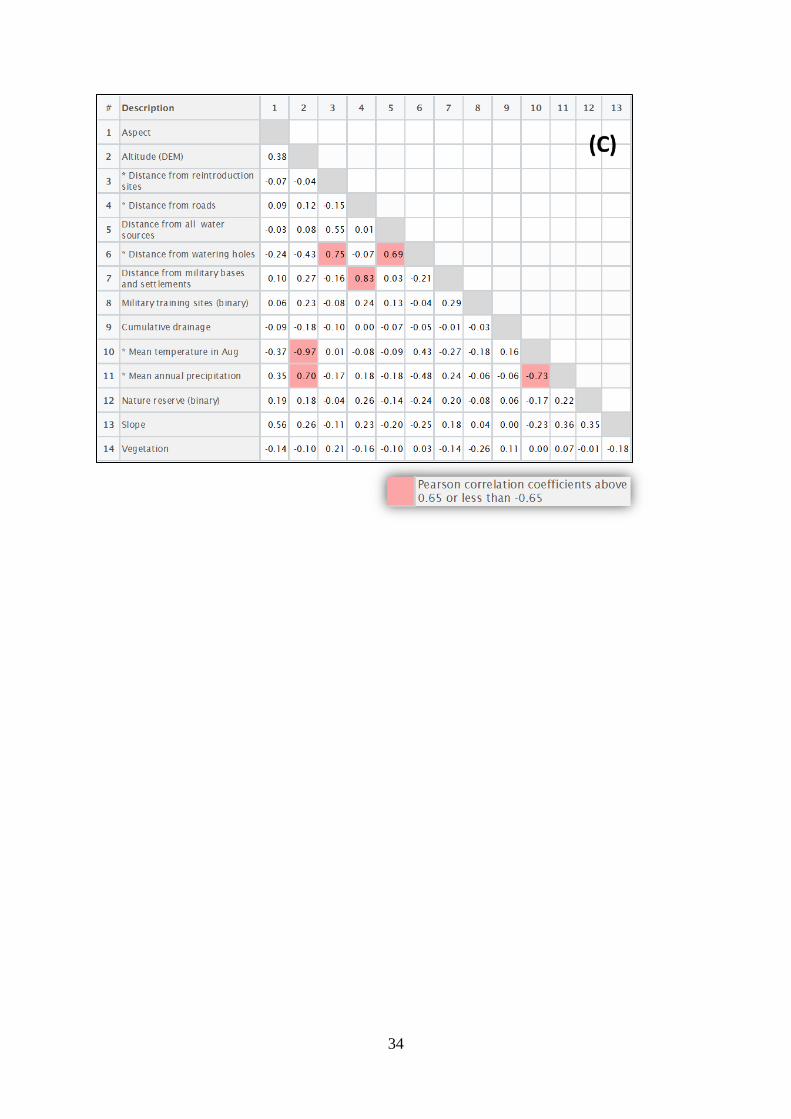
Appendix 3: Multicollinearity matrices
Table S2. Multicollinearity matrices for the variables used in the three models. (A) 10 m
resolution. (B) 100 m resolution. (C) 1000 m resolution. Stars (*) indicate variables
eliminated from the model due to high correlation with other variables.
34

35
Appendix 4: Jackknife test of variable importance (a MAXENT output)
Figure S1. Results of the Training gain jackknife test of variable importance.
Figure S2. Results of the Test gain jackknife test of variable importance.

36
Figure S3. Results of the Test AUC jackknife test of variable importance.
The environmental variable with highest Training\Test gain and Test AUC when used in
isolation is Vegetation, which therefore appears to have the most useful information by itself.
The environmental variable that decreases the Training\Test gain and Test AUC the most
when it is omitted is Vegetation, which therefore appears to have the most information that
isn't present in the other variables.

37
Appendix 5: Response curves
Figure S4. Marginal response curves of the predicted probability of wild ass occurrences for
predictor variables that contributed substantially to the distribution models. The y-axis is the
predicted probability of suitable conditions as given by the logistic output format, with all
other variables set to their average value over the set of presence localities. (A) Response of
wild ass to woody vegetation cover. (B) Response of wild ass to slope.