sage aviation’s global emissions s · system for assessing aviation’s global emissions (sage),...
TRANSCRIPT

September 2005
Brian Kim, Gregg Fleming, Sathya Balasubramanian, Andrew Malwitz, and Joosung LeeVolpe National Transportation Systems CenterEnvironmental Measurements and Modeling DivisionCambridge, MA
Ian Waitz and Kelly KlimaMassachusetts Institute of TechnologyDepartment of Aeronautics and AstronauticsCambridge, MA
Maryalice Locke, Curtis Holsclaw, Angel Morales, Edward McQueen, and Warren GilletteFederal Aviation AdministrationOffice of Environment and EnergyWashington, DC
Federal Aviation AdministrationOffice of Environment and Energy
SAGESAGEVersion 1.5
Federal Aviation AdministrationOffice of Environment and Energy
Version 1.5
Global Aviation Emissions Inventories for 2000 through 2004Global Aviation Emissions Inventories for 2000 through 2004
System for assessingAviation’s Global EmissionsSystem for assessingAviation’s Global Emissions
FAA-EE-2005-02FAA-EE-2005-02

NOTICE
This document is disseminated under the sponsorship of the Department
of Transportation in the interest of information exchange. The United
States Government assumes no liability for its contents or use
thereof. This report does not constitute a standard, specification,
or regulation.
The United States Government does not endorse products or
manufacturers. Trade or manufacturers' names appear herein solely
because they are considered essential to the object of this document.

NSN 7540-01-280-5500 Standard Form 298 (Rev. 2-89)Prescribed by ANSI Std. 239-18
298-102
REPORT DOCUMENTATION PAGE Form ApprovedOMB No. 0704-0188
Public reporting burden for this collection of information is estimated to average one hour per response, including the
time for reviewing instructions, searching existing data sources, gathering and maintaining the data needed, and completing and reviewing the collection of information. Send comments regarding this burden estimate or any other aspect of this collection of information, including suggestions for reducing this burden, to Washington Headquarters Services, Directorate for Information Operations and Reports, 1215 Jefferson Davis Highway, Suite 1204, Arlington, VA 22202-4302, and to the Office of Management and Budget, Paperwork Reduction Project (0704-0188), Washington, DC 20503.1. AGENCY USE ONLY (Leave blank) 2. REPORT DATE
September 2005 (Revised Jan-2006 & March-2008)
3. REPORT TYPE AND DATES COVEREDFinal Report – September 2005(Revised January-2006 & March-2008)
4. TITLE AND SUBTITLE
System for assessing Aviation’s Global Emissions (SAGE),Version 1.5, Global Aviation Emissions Inventories for 2000 through 2004
6. AUTHOR(S)Brian Y. Kim(1), Gregg Fleming(1), Sathya Balasubramanian(1), Andrew Malwitz(1), Joosung Lee(1), Ian Waitz(2), Kelly Klima(2), Maryalice Locke(3), Curtis Holsclaw(3), Angel Morales(3), Edward McQueen(3), Warren Gillette(3)
5. FUNDING NUMBERS
FA5N/BS043
7. PERFORMING ORGANIZATION NAME(S) AND ADDRESS(ES)
(1) U.S. Department of Transportation (2) Massachusetts Institute of Technology Research and Innovative Technology Administration Department of Aeronautics and Astronautics John A. Volpe National Transportation Systems Center Cambridge, MA 02142 Environmental Measurement and Modeling Division, DTS-34 55 Broadway Cambridge, MA 02142
8. PERFORMING ORGANIZATION REPORT NUMBER
DOT-VNTSC-FAA-05-17
9. SPONSORING/MONITORING AGENCY NAME(S) AND ADDRESS(ES)
(3) Federal Aviation Administration Office of Environment and Energy 800 Independence Ave., S.W. Washington, DC 20591
10. SPONSORING/MONITORING AGENCY REPORT NUMBER
FAA-EE-2005-02
11. SUPPLEMENTARY NOTES: FAA AEE Emissions Division Office Manager: Curtis Holsclaw FAA AEE Program Manager: Maryalice Locke
Revised January-2006 to correct page numbering errorsRevised March-2008 to correct the labeling and ordering of data in Appendices B and C.
12a. DISTRIBUTION/AVAILABILITY STATEMENT: Publicly Available 12b. DISTRIBUTION CODE
13. ABSTRACT (Maximum 200 words)
The United States (US) Federal Aviation Administration (FAA) Office of Environment and Energy (AEE) developed the System for assessing Aviation’s Global Emissions (SAGE) with support from the Volpe National Transportation Systems Center (Volpe), the Massachusetts Institute of Technology (MIT) and the Logistics Management Institute (LMI). SAGE is a high fidelity computer model used to predict aircraft fuel burn and emissions for all commercial (civil) flights globally in a given year. The model can analyze scenarios from a single flight to airport, country, regional, and global levels. In addition, SAGE dynamically models aircraft performance, fuel burn and emissions, capacity and delay at airports, and forecasts of future scenarios. The purpose of SAGE is to provide FAA, and indirectly the international aviation community, with a tool to evaluate the effects of various policy, technology, and operational scenarios on aircraft fuel use and emissions. Currently at Version 1.5, SAGE is not for use on a stand alone personal computer; it is an FAA government research tool, not for release to the public. However, results from the model have been made available to the international aviation community; and, FAA is committed to the continued development, support and reporting of SAGE.
SAGE Version 1.5 has been used to generate global inventories of fuel burn and emissions for years 2000 through 2004. These historical inventories were developed by modeling high-resolution gate-to-gate movements of all global commercial flights in each year. This report presents the inventory data in various forms and also provides derivative metrics and comparative assessments.
14. SUBJECT TERMS
SAGE, aircraft, fuel burn, emissions, emissions inventory, aircraft performance, global flights, computer model, emissions model, world fleet,
15. NUMBER OF PAGES
481
forecasting, capacity and delay, aircraft movements, bunker 16. PRICE CODE
17. SECURITY CLASSIFICATION OF REPORT
Unclassified
18. SECURITY CLASSIFICATION OF THIS PAGE
Unclassified
19. SECURITY CLASSIFICATION OF ABSTRACT
Unclassified
20. LIMITATION OF ABSTRACT

SAGE Version 1.5 – Global Aviation Emissions Inventories for 2000 through 2004 September 2005
TABLE OF CONTENTS
1 Introduction................................................................................................................................................ 11.1 Background......................................................................................................................................... 11.2 Objective and Scope ........................................................................................................................... 21.3 Modeling Capabilities......................................................................................................................... 21.4 Document Outline............................................................................................................................... 3
2 Raw Inventory Descriptions ...................................................................................................................... 42.1 Raw Flight-Level Modal Inventory .................................................................................................... 42.2 Raw Chord-Level Inventory............................................................................................................... 62.3 Raw 4D World Gridded Inventory ..................................................................................................... 7
3 Processed Inventories................................................................................................................................. 93.1 Regional and Country Inventories.................................................................................................... 103.2 Aircraft Inventories........................................................................................................................... 223.3 Gridded Inventories .......................................................................................................................... 29
4 Comparisons to Past Inventories.............................................................................................................. 355 Conclusions.............................................................................................................................................. 41References................................................................................................................................................... 42APPENDIX A: Processed Regional Inventories…………………………………………………………45APPENDIX B: Processed Country Inventories…………………………………………………………..52APPENDIX C: Processed Aircraft-Engine Inventories…………………………………………………. 71APPENDIX D: Processed Modal Aircraft Inventories………………………………………………….223
LIST OF TABLES
Table 1. Yearly Global Total Fuel Burn and Emissions .............................................................................. 9Table 2. Yearly Global Derived Metrics of Fuel Efficiency and Emissions Indices ................................... 9Table 3. Landing and Takeoff (LTO) and Cruise Fuel Burn and NOx Emissions .................................... 10Table 4. Global Fuel Burn and NOx Emissions Separated into Jet and Turboprop categories. ................ 10Table 5. Yearly Regional Totals for Fuel Burn (Tg) ................................................................................. 12Table 6. Yearly Regional Totals for NOx Emissions (Tg) ........................................................................ 12Table 7. Regional Fuel Burn per Distance (Tg/Billion km)....................................................................... 15Table 8. Regional Fuel Burn per Flight (Mg/Flight)..................................................................................15Table 9. Regional NOx Emissions per Distance (Tg/Billion km).............................................................. 16Table 10. Regional NOx Emissions per Flight (Kg/Flight) ....................................................................... 16Table 11. Yearly Total Fuel Burn by Country (Gg)...................................................................................17Table 12. Yearly Total NOx Emissions by Country (Gg) ......................................................................... 19Table 13. Jet and Turboprop Global Totals ............................................................................................... 22Table 14. Jet and Turboprop Global Derived Metrics ............................................................................... 22Table 15. Aircraft Accounting for 95% of Global Total Flights................................................................ 23Table 16. Aircraft Accounting for 95% of Global Total Distance Flown.................................................. 25Table 17. Aircraft Accounting for 95% of Global Total Fuel Burn........................................................... 26Table 18. Aircraft Accounting for 95% of Global Total NOx Emissions.................................................. 27

SAGE Version 1.5 – Global Aviation Emissions Inventories for 2000 through 2004 September 2005
LIST OF FIGURES
Figure 1. Raw and Processed Inventories .................................................................................................... 4Figure 2. Orientation of Standard Grids within SAGE................................................................................ 8Figure 3. Worldwide Airport Locations Color-Coded by Region ............................................................. 11Figure 4. Comparison of Regional Domestic Fuel Burn............................................................................ 13Figure 5. Comparison of Regional International Fuel Burn ...................................................................... 13Figure 6. Comparison of Regional Domestic NOx Emissions .................................................................. 14Figure 7. Comparison of Regional International NOx Emissions ............................................................. 14Figure 8. Trends in Domestic Fuel Burn for Selected Countries............................................................... 20Figure 9. Trends in International Fuel Burn for Selected Countries.......................................................... 21Figure 10. Trends in Total (Domestic plus International) Fuel Burn for Selected Countries.................... 21Figure 11. Gridded Plot of Global Fuel Burn for 2000 with all Altitudes Aggregated ............................. 30Figure 12. Gridded Plot of North American Fuel Burn for 2000 with all Altitudes Aggregated .............. 30Figure 13. Gridded Plot European Fuel Burn for 2000 with all Altitudes Aggregated ............................. 31Figure 14. Gridded Plot of Asian Fuel Burn for 2000 with all Altitudes Aggregated ............................... 31Figure 15. Altitude Distribution of Fuel Burn and Emissions for Year 2000............................................ 32Figure 16. Distribution of Fuel Burn and Emissions by Longitude ........................................................... 33Figure 17. Distribution of Fuel Burn and Emissions by Latitude .............................................................. 33Figure 18. Relative Loadings of Fuel Burn and Emissions by World Quadrant ....................................... 34Figure 19. Comparison of Fuel Burn from Past Studies ............................................................................ 35Figure 20. Comparison of CO2 Emissions from Past Studies.................................................................... 36Figure 21. Comparison of NOx Emissions from Past Studies ................................................................... 36Figure 22. Comparison of CO Emissions from Past Studies ..................................................................... 37Figure 23. Comparison of HC Emissions from Past Studies ..................................................................... 37Figure 24. Comparison of SAGE Global Average NOx EI Values with Past Studies .............................. 38Figure 25. Comparison of SAGE Global Average CO EI Values with Past Studies................................. 39Figure 26. Comparison of SAGE Global Average HC EI Values with Past Studies................................. 39Figure 27. Comparison of Cruise (> 1 km Altitude above airport field elevation) NOx EI Values by
Selected Aircraft Types from SAGE 2000 and NASA/Boeing 1999 Inventories.............................. 40

SAGE Version 1.5 – Global Aviation Emissions Inventories for 2000 through 2004 September 2005
LIST OF ACRONYMS
4D Four-DimensionalAEE Office of Environment and EnergyBACK BACK Aviation SolutionsBADA Base of Aircraft DataCAEP Committee on Aviation Environmental ProtectionCDA Continuous Descent ApproachCNS Communication, Navigation, and SurveillanceEDMS Emissions and Dispersion Modeling SystemEI Emissions IndexETMS Enhanced Traffic Management SystemEurocontrol European Organization for the Safety of Air NavigationFAA Federal Aviation AdministrationGC Great CircleICAO International Civil Aviation OrganizationLMI Logistics Management InstituteLTO Landing and TakeoffNASA National Aeronautics and Space AdministrationOAG Official Airline GuideRVSM Reduced Vertical Separation MinimumUN United NationsUNFCCC United Nations Framework Convention on Climate ChangeUS United States

SAGE Version 1.5 – Global Aviation Emissions Inventories for 2000 through 2004 September 2005
1
1 Introduction
The United States (US) Federal Aviation Administration (FAA) Office of Environment and Energy (AEE) developed the System for assessing Aviation’s Global Emissions (SAGE) with support from the Volpe National Transportation Systems Center (Volpe), the Massachusetts Institute of Technology (MIT) and the Logistics Management Institute (LMI). SAGE is a high fidelity computer model used to predict aircraft fuel burn and emissions for all commercial (civil) flights globally in a given year. The model can analyze scenarios from a single flight to airport, country, regional, and global levels. In addition, SAGE dynamically models aircraft performance, fuel burn and emissions, capacity and delay at airports, and forecasts of future scenarios. The purpose of SAGE is to provide FAA, and indirectly the international aviation community, with a tool to evaluate the effects of various policy, technology, and operational scenarios on aircraft fuel use and emissions. Currently at Version 1.5, SAGE is not for use on a stand alone personal computer; it is an FAA government research tool, not for release to the public. However, results from the model have been made available to the international aviation community; and, FAA is committed to the continued development, support and reporting of SAGE.
SAGE Version 1.5 has been used to generate global inventories of fuel burn and emissions for years 2000 through 2004. These historical inventories were developed by modeling high-resolution gate-to-gate movements of all global commercial flights in each year. This report presents the inventory data in various forms and also provides derivative metrics and comparative assessments. As this report is intended to present inventory data, technical model details and validation assessments are not discussed. Such details can be found in FAAa 2005 and FAAb 2005.
The inventory data presented in this report represents condensed (e.g., aggregated) versions of the raw inventory outputs from SAGE which range from inventories with tens of millions of records to those with approximately a billion records of detailed flight results for each modeled year. Significant resources are expended in generating these raw inventories and the condensed, derived data.
As a formal disclaimer, any SAGE data including those contained in this report are made available to interested parties as is. FAA is not liable for any misunderstandings and misuses of the data. The user is solely responsible for any consequences arising from inappropriate application of the data.
1.1 Background
The development of SAGE was in part stimulated by the rapid growth in aviation and the need for better emissions modeling capabilities on a global level. According to the “Special Report on Aviation and the Global Atmosphere” by the Intergovernmental Panel on Climate Change (IPCC), air transportation accounted for 2 percent of all anthropogenic carbon dioxide emissions in 1992 and 13 percent of the fossil fuel used for transportation. In a 10-year period, passenger traffic on scheduled airlines grew by 60 percent; and, air travel was expected to increase by 5 percent for the next 10 to 15 years [IPCC 1999]. With this forecast, aircraft remain an important source of greenhouse gases in coming decades [IPCC 1999]. It was also estimated that in 1992, aircraft were responsible for 3.5 percent of all anthropogenic radiative forcing of the climate and (at the time of the report, were) expected to grow to as much as 12 percent by 2050 [IPCC 1999].
The Committee on Aviation Environmental Protection (CAEP) of the International Civil Aviation Organization (ICAO), an organization of the United Nations (UN), has formed several working groups to address aviation environmental emissions. In addition, the UN Framework Convention on Climate
SAGE Version 1.5 – Global Aviation Emissions Inventories for 2000 through 2004 September 2005
2
Change (UNFCCC) has promoted a series of multilateral agreements that target values of emissions reductions for the primary industrialized nations [IPCC 1999]. However, prior to SAGE, there was no comprehensive, up-to-date, non-proprietary model to estimate aviation emissions at national or international levels that could be used for evaluating policy, technology and operational alternatives.
Although the degree of projected growth of the air transportation industry may be debated, the unique characteristics of the industry, the influence that they may have upon the environment, and the influence that policies may have upon the industry dictates a clear need for a computer model that analysts can use to predict and evaluate the effects of different policy, technology, and operational scenarios.
Past studies on aircraft emissions have resulted in global inventories of emissions by various organizations including the National Aeronautics and Space Administration (NASA)/Boeing [Baughcum 1996a,b and Sutkus 2001], Abatement of Nuisance Caused by Nuisances Caused by Air Transport (ANCAT)/European Commission (EC) 2 group [Gardner 1998], and Deutsche Forschungsanstalt fur Luft- and Raumfahrt (DLR) [Schmitt 1997]. These inventories represent significant accomplishments since they are the first set of “good-quality” global emissions estimates. In this light, SAGE represents the lessons learned from these past studies. Using the best publicly available data and methods, SAGE improves upon these past studies in producing the highest quality emissions inventories to date.
1.2 Objective and Scope
The objective for SAGE is to be an internationally accepted computer model that is based on the best publicly available data and methodologies, and that can be used to estimate the effects on global aircraft fuel burn and emissions from various policy, technology, and operational scenarios. With regard to scope, the model is capable of analyses from a single flight to airport, regional, and global levels of commercial (civil) flights on a worldwide basis.
1.3 Modeling Capabilities
With the computation modules and the supporting data integrated in a dynamic modeling environment, SAGE provides the capability to model changes to various parameters including those associated with flight schedules, trajectories, aircraft performance, airport capacities and delays, etc. This results in the ability to use SAGE for applications such as quantification of the effects of Communication, Navigation, and Surveillance (CNS)/Air Traffic Management (ATM) initiatives, determining the benefits of Reduced Vertical Separation Minimum (RVSM), investigation of trajectory optimizations, and computing potential emissions benefits from the use of a Continuous Descent Approach (CDA).
SAGE can generate inventories of fuel burn and emissions of carbon monoxide (CO), unburned hydrocarbons (HC), nitrogen oxides (NOx), carbon dioxide (CO2), water (H2O), and sulfur oxides (SOx calculated as sulfur dioxide, SO2). The three basic inventories generated by SAGE are: (1) four-dimensional (4D) variable world grids currently generated in a standardized 1o latitude by 1o longitude by 1 km altitude format; (2) modal results of each individual flight worldwide; and (3) individual chorded (flight segment) results for each flight worldwide. These outputs and the dynamic modeling environment allow for a comprehensive set of analyses that can be conducted using SAGE.

SAGE Version 1.5 – Global Aviation Emissions Inventories for 2000 through 2004 September 2005
3
1.4 Document Outline
The remainder of this document is organized as follows. Section 2 defines and discusses the raw inventories generated by the model. This section serves as background material for the subsequent sections. Section 3 describes the various processed inventories which provide more meaningful information. Section 4 presents comparisons of SAGE data with those from past studies. Finally, Section 5 provides concluding remarks related to these inventories generated by SAGE Version 1.5.

SAGE Version 1.5 – Global Aviation Emissions Inventories for 2000 through 2004 September 2005
4
2 Raw Inventory Descriptions
The basic outputs from SAGE are fuel burn and emissions of CO, HC, NOx, CO2, H2O, and SOx (modeled as SO2). These data and others are generated by SAGE as part of three raw inventories as shown in Figure 1: (1) flight-level modal, (2) chord-level, and (3) 4D world grids.
SAGE
Raw Fuel Burn and Emissions Results
Flight Level Modal Chord Level 4D World Grids
Figure 1. Raw and Processed Inventories
These three inventories are generated for each year and stored in a relational database (i.e., SQL database). Currently, inventories have been generated for five years: 2000 through 2004. Sections 2.1 through 2.3 describe each of these inventories. These descriptions are provided as background material and to serve as the basis for further discussions and presentations of the processed data in the ensuing sections.
2.1 Raw Flight-Level Modal Inventory
The flight-level modal inventory contains listings of each individual civil flight on a global basis. This inventory contains over 30 millions per year. These results are provided modally as indicated by the fields shown below:
flight_key = unique SAGE flight key flight_date = flight departure date source_flag = E=Enhanced Traffic Management System (ETMS),
O=Official Airline Guide (OAG) flight_id = flight ID status_flag = internal debugging flag dep_airport = departure airport code arr_airport = arrival airport code dep_time = departure time arr_time = arrival time cruise_altitude (ft) = cruise altitude track_no = dispersion track number for OAG flights aircraft_type = aircraft code

SAGE Version 1.5 – Global Aviation Emissions Inventories for 2000 through 2004 September 2005
5
aircraft_category = J=Jet, T=Turboprop, P=Piston num_engines = number of engines back_engine = BACK Aviation’s Fleet data engine name/code icao_edms_engine = ICAO or FAA’s Emissions and Dispersion
Modeling System (EDMS) engine name/code gc_distance (nm) = Great Circle (GC) distance flight_distance (nm) = flight distance carrier_code = carrier code carrier_name = carrier name region_code = region code (8 world regions) region_name = region name (8 world regions) region_end_type = I=flight ended in same region, O=ended
elsewhere dep_country = departure country name arr_country = arrival country name takeoff_weight (kg) = assigned takeoff weight scale_factor = scale factor for unscheduled flights dep_gnd_distance (nm) = departure ground distance dep_gnd_fuelburn (kg) = departure ground fuel burn dep_gnd_co2 (g) = departure ground CO2
dep_gnd_h2o (g) = departure ground H2O dep_gnd_sox (g) = departure ground SOx dep_gnd_co (g) = departure ground CO dep_gnd_hc (g) = departure ground HC dep_gnd_nox (g) = departure ground NOx to_co_distance (nm) = takeoff/climbout distance to_co_fuelburn (kg) = takeoff/climbout fuel burn to_co_co2 (g) = takeoff/climbout CO2
to_co_h2o (g) = takeoff/climbout H2O to_co_sox (g) = takeoff/climbout SOx to_co_co (g) = takeoff/climbout CO to_co_hc (g) = takeoff/climbout HC to_co_nox (g) = takeoff/climbout NOx cruise_distance (nm) = cruise distance cruise_fuelburn (kg) = cruise fuelf burn cruise_co2 (g) = cruise CO2
cruise_h2o (g) = cruise H2O cruise_sox (g) = cruise SOx cruise_co (g) = cruise CO cruise_hc (g) = cruise HC cruise_nox (g) = cruise NOx app_glide_distance (nm) = approach distance app_glide_fuelburn (kg) = approach fuel burn app_glide_co2 (g) = approach CO2
app_glide_h2o (g) = approach H2O
SAGE Version 1.5 – Global Aviation Emissions Inventories for 2000 through 2004 September 2005
6
app_glide_sox (g) = approach SOx app_glide_co (g) = approach CO app_glide_hc (g) = approach HC app_glide_nox (g) = approach NOx arr_gnd_distance (nm) = arrival ground distance arr_gnd_fuelburn (kg) = arrival ground fuel burn arr_gnd_co2 (g) = arrival ground CO2
arr_gnd_h2o (g) = arrival ground H2O arr_gnd_sox (g) = arrival ground SOx arr_gnd_co (g) = arrival ground CO arr_gnd_hc (g) = arrival ground HC arr_gnd_nox (g) = arrival ground NOx fuelburn (kg) = total fuel burn co2 (g) = total CO2
h2o (g) = total H2O sox (g) = total SOx co (g) = total CO hc (g) = total HC nox (g) = total NOx
Regarding the definition for modes, 3000 ft is used to differentiate cruise from takeoff/climbout and approach. This inventory provides enough details for most comparison and trend analyses by regional, country, airport, and aircraft levels.
Due to the large uncertainties associated with emissions indices (EI) for piston engines, flights with aircraft using piston engines have been flagged in this inventory. These flights are currently excluded when the data is used to generate more meaningful aggregated results (e.g., regional, country, etc. totals).
2.2 Raw Chord-Level Inventory
The chord-level inventory contains a listing of individual flight chords for all flights worldwide resulting in approximately 1 billion yearly records. Even though each listing represents a point in space geometrically, it can be considered to represent a chord (or segment) because much of the information provided in the inventory necessarily apply to the entire chord rather than just a point. For clarity, the ends of a chord are referred to as either the head (beginning) or tail (ending) points. And it should be obvious that the tail point of one chord represents the head point of the next chord. Whether the data in the inventory applies to a point or the entire chord, the information is always stored at the tail point of the chord. The fields within this inventory are provided as follows:
flight_key = unique SAGE flight key seq_no = chord sequence number mode = mode number for chord latitude (deg) = latitude of chord tail longitude (deg) = longitude of chort tail altitude (m) = altitude of chord tail chord_time = point in time at chord tail T_i (K) = temperature at chord tail

SAGE Version 1.5 – Global Aviation Emissions Inventories for 2000 through 2004 September 2005
7
P_i (Pa) = pressure at chord tail a_i (m/s) = speed of sound at chord tail m_i = average Mach number for chord h_i (m) = average height of chord delta_alt (m) = change in altitude for chord v_i (m/s) = average speed of chord delta_v (m/s) = change in speed for chord delta_t (s) = change in time for chord distance (nm) = length of chord thrust (N) = thrust for the chord weight (kg) = aircraft weight at chord tail cl_i = Eurocontrol’s Base of Aircraft data (BADA) lift coefficient for chord cd_i = BADA drag coefficient for chord l_i (N) = lift force for chord d_i (N) = drag force for chord f_i (kg/s) = fuel flow for chord percent_foo = percent power for chord reico_i (g/kg-fuel) = corrected (reference) CO emissions index (EI) for chord reihc_i (g/kg-fuel) = corrected (reference) HC EI for chord reinox_i (g/kg-fuel) = corrected (reference) NOx EI for chord fuelburn (kg) = fuel burned for chord co2 (g) = CO2 emitted for chord h2o (g) = H2O emitted for chord sox (g) = SOx emitted for chord co (g) = CO emitted for chord hc (g) = HC emitted for chord nox (g) = NOx emitted for chord
This inventory has typically been used for model improvements, validation, and detailed scenario modeling, especially those involving modifications to aircraft performance parameters.
2.3 Raw 4D World Gridded Inventory
The 4D world grid inventory contains a listing of flight segments similar to the chord-level inventory but the segments correspond to the portions of the chords that traversed a grid. The data is 4D since each segment listing contains flight date/time and grid location information. The similarity to the chord-level inventory is reflected by the approximately 900 million yearly records within this inventory. The fields in the inventory are shown below:
flight_key = unique SAGE flight key flight_date = departure date track_id = dispersion track number for OAG flights seq_no = chord sequence number mode = mode number i = latitude index j = longitude index k = altitude index

SAGE Version 1.5 – Global Aviation Emissions Inventories for 2000 through 2004 September 2005
8
time_in = time entered into grid deltat_i (s) = duration in grid v_i (m/s) = average speed of chord fuelburn (kg) = fuel burned while in grid co2 (g) = CO2 emitted while in grid h2o (g) = H2O emitted while in grid co (g) = CO emitted while in grid sox (g) = SOx emitted while in grid hc (g) = HC emitted while in grid nox (g) = NOx emitted while in grid
The current standard grid size is 1o latitude by 1o longitude by 1 km altitude. But these specifications can be modified to obtain varying sizes in all three dimensions. The i, j, and k indices used in this inventory are based on the standard grid cell size, and their orientation is shown in Figure 2.
Lon = 0Lon = -180
Lon = 180Lat = 0
Lat = -90
[0, 90]
[0, 0]
[1, 0]
[0, 1]
[0, 91]
[1, 90]
[179, 0]
[178, 0]
[179, 1]
[0, 179]
[179, 90]
[179, 178]
[179, 179][178, 179]
[359, 0]
[180, 0]
[180, 179]
[180, 1]
[181, 0]
[181, 179]
[180, 178]
Lat = 90
[359, 179]
[358, 179]
[359, 178]
j
i[j, i]
Lat = 0Lat = 0
Lon = 0
Lon = 0
[359, 88]
[359, 89]
[358, 89]
Figure 2. Orientation of Standard Grids within SAGE
This inventory provides the data necessary to assess the spatial and temporal distributions of fuel burn and emissions. The potential exists for the data to serve as inputs to atmospheric dispersion and global warming models.
SAGE Version 1.5 – Global Aviation Emissions Inventories for 2000 through 2004 September 2005
9
3 Processed Inventories
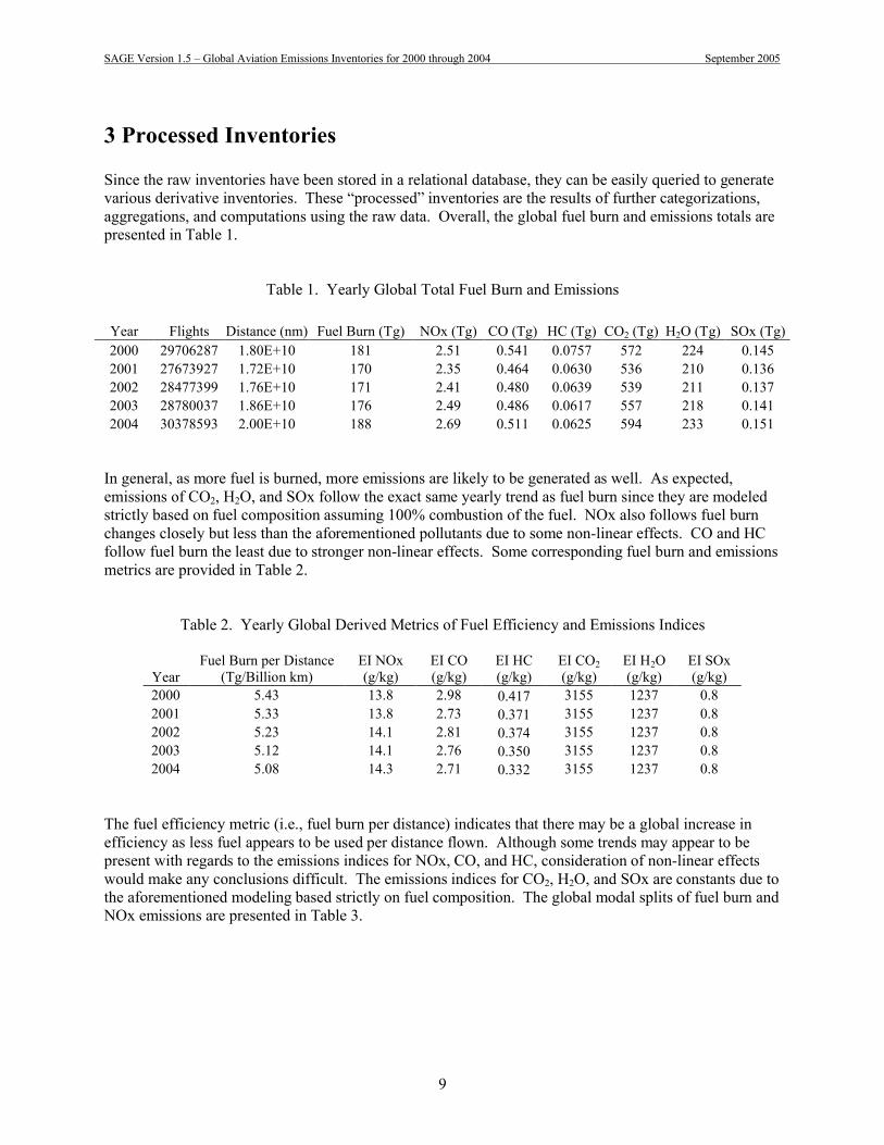
Since the raw inventories have been stored in a relational database, they can be easily queried to generate various derivative inventories. These “processed” inventories are the results of further categorizations, aggregations, and computations using the raw data. Overall, the global fuel burn and emissions totals are presented in Table 1.
Table 1. Yearly Global Total Fuel Burn and Emissions
Year Flights Distance (nm) Fuel Burn (Tg) NOx (Tg) CO (Tg) HC (Tg) CO2 (Tg) H2O (Tg) SOx (Tg)2000 29706287 1.80E+10 181 2.51 0.541 0.0757 572 224 0.1452001 27673927 1.72E+10 170 2.35 0.464 0.0630 536 210 0.1362002 28477399 1.76E+10 171 2.41 0.480 0.0639 539 211 0.1372003 28780037 1.86E+10 176 2.49 0.486 0.0617 557 218 0.1412004 30378593 2.00E+10 188 2.69 0.511 0.0625 594 233 0.151
In general, as more fuel is burned, more emissions are likely to be generated as well. As expected, emissions of CO2, H2O, and SOx follow the exact same yearly trend as fuel burn since they are modeled strictly based on fuel composition assuming 100% combustion of the fuel. NOx also follows fuel burn changes closely but less than the aforementioned pollutants due to some non-linear effects. CO and HC follow fuel burn the least due to stronger non-linear effects. Some corresponding fuel burn and emissions metrics are provided in Table 2.
Table 2. Yearly Global Derived Metrics of Fuel Efficiency and Emissions Indices
YearFuel Burn per Distance
(Tg/Billion km)EI NOx (g/kg)
EI CO (g/kg)
EI HC (g/kg)
EI CO2
(g/kg)EI H2O (g/kg)
EI SOx (g/kg)
2000 5.43 13.8 2.98 0.417 3155 1237 0.82001 5.33 13.8 2.73 0.371 3155 1237 0.82002 5.23 14.1 2.81 0.374 3155 1237 0.82003 5.12 14.1 2.76 0.350 3155 1237 0.82004 5.08 14.3 2.71 0.332 3155 1237 0.8
The fuel efficiency metric (i.e., fuel burn per distance) indicates that there may be a global increase in efficiency as less fuel appears to be used per distance flown. Although some trends may appear to be present with regards to the emissions indices for NOx, CO, and HC, consideration of non-linear effects would make any conclusions difficult. The emissions indices for CO2, H2O, and SOx are constants due to the aforementioned modeling based strictly on fuel composition. The global modal splits of fuel burn and NOx emissions are presented in Table 3.

SAGE Version 1.5 – Global Aviation Emissions Inventories for 2000 through 2004 September 2005
10
Table 3. Landing and Takeoff (LTO) and Cruise Fuel Burn and NOx Emissions
Fuel Burn (Tg) NOx (Tg)Year LTO Cruise LTO Cruise2000 12.9 168 0.197 2.312001 12.3 158 0.191 2.162002 12.2 159 0.194 2.222003 12.4 164 0.199 2.292004 12.9 175 0.210 2.48
As discussed in Section 2.1, 3000 ft altitude is used to differentiate between the landing and takeoff (LTO) cycle and cruise. Specifically, the definition for the LTO cycle category is all fuel burn and emissions generated equal to or below 3000 ft above airport field elevation (AFE). Consequently, cruise is defined as all fuel burn and emissions generated above 3000 ft AFE. Since NOx tends to follow fuel burn trends well, the cruise to LTO ratios are both similar for fuel burn (about 13) and NOx (about 11.5). These ratios are approximately constant for each of the five years.
The global fuel burn and emissions separated into jet and turboprop categories are shown in Table 4.
Table 4. Global Fuel Burn and NOx Emissions Separated into Jet and Turboprop categories.
Fuel Burn (Tg) NOx (Tg)Year Jet Turboprop Jet Turboprop2000 177 4.25 2.45 0.05692001 166 3.48 2.30 0.04862002 167 3.51 2.37 0.04852003 173 3.28 2.45 0.04702004 185 3.28 2.64 0.0468
As discussed in Section 2.1, the turboprop category does not include piston-powered aircraft as these have been excluded due to the uncertainties associated with their emissions data. As expected, the jet contribution to global fuel burn and NOx emissions is far greater than turboprops due to the greater number of jet operations as well as the higher fuel burn on a per flight basis. Similar to the cruise and LTO comparisons, the jet to turboprop ratio is also similar when comparing fuel burn and NOx. However, the ratios appear to be different from year to year. The ratios increase from about 42-43 to about 56, possibly indicating an increase in jet usage or a decrease in turboprop usage.
3.1 Regional and Country Inventories
The SAGE flight-level modal inventory was processed to derive regional and country inventories. The attribution of fuel burn and emissions to a region or country is mainly based on the location (or ownership) of the departure airport. Figure 3 shows a plot to illustrate the worldwide locations of airports color-coded by region.

SAGE Version 1.5 – Global Aviation Emissions Inventories for 2000 through 2004 September 2005
11
Figure 3. Worldwide Airport Locations Color-Coded by Region
All fuel burn and emissions for a flight are attributed to the country/region containing the airport and is either categorized as domestic or international depending on whether or not the arrival airport is within the same country/region. The following examples illustrate this definition:
Flight 1: Country A, Domestico Departure airport in country Ao Arrival airport in country A
Flight 2: Country A, Internationalo Departure airport in country Ao Arrival airport in country B
The fuel burn and emissions resulting from flight 1 are attributed to the country A, domestic category because both the departure and arrival airports are in country A. In contrast, the fuel burn and emissions for flight 2 are categorized into the country A, international category because the arrival airport is not within country A. That is, any country other than A would result in the same international classification. In accordance with the terminology often used by UNFCCC, the international category can also be referred to as a “bunker” category [IPCC 1997].
As indicated in Figure 3, the SAGE data are typically aggregated into the following eight world regions: Africa Asia Australia and Oceania Eastern Europe Middle East North America and Caribbean South America Western Europe and North Atlantic

SAGE Version 1.5 – Global Aviation Emissions Inventories for 2000 through 2004 September 2005
12
The allocation of countries to each of these regions can be found in FAAa 2005. The regional inventories subdivided into domestic versus international and modal categories for 2000 to 2004 are provided in Appendix A. Based on this data, the yearly regional totals for fuel burn and NOx are presented in Tables 4 and 5 with corresponding plots shown in Figures 4 through 7.
Table 5. Yearly Regional Totals for Fuel Burn (Tg)
Type Region 2000 2001 2002 2003 2004Africa 1.12 1.15 1.14 1.19 1.25Asia 16.8 17.7 18.4 19.2 21.3
Australia and Oceania 2.39 2.44 2.29 2.12 2.31Eastern Europe 1.88 2.03 2.04 2.26 2.45
Middle East 2.46 2.39 2.37 2.57 2.83North America and Caribbean 62.9 57.4 55.1 56.1 56.5
South America 3.27 3.41 3.40 3.06 3.21
Domestic
Western Europe and North Atlantic 13.6 12.7 13.9 15.3 16.1Africa 2.42 2.38 2.56 2.64 2.86Asia 15.9 15.2 15.4 15.8 17.5
Australia and Oceania 2.86 2.62 2.66 2.72 3.15Eastern Europe 2.06 2.01 2.09 2.39 2.81
Middle East 5.08 4.98 4.81 5.40 6.45North America and Caribbean 22.7 18.2 19.7 19.9 21.3
South America 3.31 2.98 3.02 2.80 3.20
International
Western Europe and North Atlantic 22.6 22.2 21.9 23.0 25.2Global Total N/A 181 170 171 176 188
Table 6. Yearly Regional Totals for NOx Emissions (Tg)
Type Region 2000 2001 2002 2003 2004Africa 0.0140 0.0142 0.0140 0.0146 0.0153Asia 0.263 0.277 0.285 0.295 0.333
Australia and Oceania 0.0337 0.0328 0.0308 0.0301 0.0332Eastern Europe 0.0165 0.0175 0.0172 0.0186 0.0193
Middle East 0.0381 0.0379 0.0380 0.0413 0.0458North America and Caribbean 0.786 0.716 0.708 0.717 0.724
South America 0.0379 0.0393 0.0424 0.0386 0.0409
Domestic
Western Europe and North Atlantic 0.167 0.159 0.178 0.196 0.210Africa 0.0353 0.0350 0.0393 0.0405 0.0440Asia 0.243 0.231 0.240 0.246 0.272
Australia and Oceania 0.0455 0.0421 0.0424 0.0432 0.0502Eastern Europe 0.0236 0.0230 0.0244 0.0287 0.0341
Middle East 0.0730 0.0732 0.0710 0.0792 0.0963North America and Caribbean 0.341 0.273 0.305 0.311 0.334
South America 0.0466 0.0432 0.0435 0.0402 0.0466
International
Western Europe and North Atlantic 0.342 0.335 0.335 0.353 0.387Global Total N/A 2.51 2.35 2.41 2.49 2.69

SAGE Version 1.5 – Global Aviation Emissions Inventories for 2000 through 2004 September 2005
13
0
10
20
30
40
50
60
70
Africa Asia Australiaand
Oceania
EasternEurope
Middle East NorthAmerica
andCaribbean
SouthAmerica
WesternEurope and
NorthAtlantic
Region
Fu
el B
urn
(T
g)
Year 2000
Year 2001
Year 2002
Year 2003
Year 2004
Figure 4. Comparison of Regional Domestic Fuel Burn
0
5
10
15
20
25
30
Africa Asia Australiaand
Oceania
EasternEurope
Middle East NorthAmerica
andCaribbean
SouthAmerica
WesternEurope and
NorthAtlantic
Region
Fu
el B
urn
(T
g) Year 2000
Year 2001
Year 2002
Year 2003
Year 2004
Figure 5. Comparison of Regional International Fuel Burn

SAGE Version 1.5 – Global Aviation Emissions Inventories for 2000 through 2004 September 2005
14
0
0.1
0.2
0.3
0.4
0.5
0.6
0.7
0.8
0.9
Africa Asia Australiaand
Oceania
EasternEurope
MiddleEast
NorthAmerica
andCaribbean
SouthAmerica
WesternEurope
and NorthAtlantic
Region
NO
x (T
g)
Year 2000
Year 2001
Year 2002
Year 2003
Year 2004
Figure 6. Comparison of Regional Domestic NOx Emissions
0
0.05
0.1
0.15
0.2
0.25
0.3
0.35
0.4
0.45
Africa Asia Australiaand
Oceania
EasternEurope
Middle East NorthAmerica
andCaribbean
SouthAmerica
WesternEurope
and NorthAtlantic
Region
NO
x (T
g)
Year 2000
Year 2001
Year 2002
Year 2003
Year 2004
Figure 7. Comparison of Regional International NOx Emissions
The comparisons in Figures 4 and 5 show that global domestic fuel burn is dominated by the North America and Caribbean region. In contrast, international fuel burn is similar among three regions: Asia, North America and Caribbean, and Western Europe and North Atlantic. The yearly trends in each of these regions generally show an increase from 2002 to 2004 to reflect the growth in the aviation industry. However, decreases shown from 2000 to the following years reflect the effects of September 11, 2001. As expected, the NOx comparisons shown in Figures 6 and 7 follow the same type of distributions as

SAGE Version 1.5 – Global Aviation Emissions Inventories for 2000 through 2004 September 2005
15
shown by the fuel burn comparisons. A couple of normalized fuel burn and NOx metrics (i.e., per distance and per NOx) are shown in Tables 7 through 10.
Table 7. Regional Fuel Burn per Distance (Tg/Billion km)
Type Region 2000 2001 2002 2003 2004Africa 4.24 3.95 3.87 3.77 3.73Asia 6.45 6.36 6.21 6.06 5.86
Australia and Oceania 3.86 3.87 3.91 3.88 3.85Eastern Europe 5.22 5.15 5.02 5.01 5.00
Middle East 5.91 5.98 6.02 6.09 6.06North America and Caribbean 4.07 3.94 3.78 3.65 3.53
South America 3.94 3.93 4.02 4.17 4.19
Domestic
Western Europe and North Atlantic 3.68 3.63 3.58 3.56 3.57Africa 8.05 8.01 8.02 7.65 7.33Asia 10.60 10.49 10.38 10.20 9.99
Australia and Oceania 9.33 9.41 8.77 8.71 8.63Eastern Europe 4.52 4.39 4.38 4.32 4.23
Middle East 7.05 7.10 6.98 6.98 7.06North America and Caribbean 8.76 8.66 8.77 8.74 8.67
South America 7.07 7.02 6.93 6.78 6.88
International
Western Europe and North Atlantic 8.09 8.09 8.03 7.90 7.74
Table 8. Regional Fuel Burn per Flight (Mg/Flight)
Type Region 2000 2001 2002 2003 2004Africa 2.99 2.80 2.83 2.87 2.89Asia 6.22 6.26 6.21 6.25 6.33
Australia and Oceania 2.85 2.99 2.97 2.99 3.06Eastern Europe 5.17 5.07 5.10 5.24 5.10
Middle East 4.79 4.82 5.03 5.26 5.41North America and Caribbean 3.82 3.89 3.68 3.74 3.62
South America 2.86 2.89 2.91 3.20 3.31
Domestic
Western Europe and North Atlantic 2.56 2.59 2.59 2.71 2.74Africa 31.8 31.0 30.6 28.9 27.8Asia 72.7 74.5 71.4 69.6 68.1
Australia and Oceania 51.5 58.7 48.7 49.1 50.0Eastern Europe 7.62 7.21 7.28 7.36 7.11
Middle East 23.5 23.6 23.2 23.4 24.3North America and Caribbean 57.1 57.7 57.0 57.9 58.0
South America 31.9 34.0 31.3 31.8 33.5
International
Western Europe and North Atlantic 35.1 34.5 33.9 32.6 31.0

SAGE Version 1.5 – Global Aviation Emissions Inventories for 2000 through 2004 September 2005
16
Table 9. Regional NOx Emissions per Distance (Tg/Billion km)
Type Region 2000 2001 2002 2003 2004Africa 0.0531 0.0490 0.0476 0.0465 0.0457Asia 0.101 0.0996 0.0964 0.0931 0.0915
Australia and Oceania 0.0544 0.0519 0.0525 0.0550 0.0555Eastern Europe 0.0458 0.0443 0.0424 0.0412 0.0393
Middle East 0.0915 0.0947 0.0964 0.0978 0.0980North America and Caribbean 0.0508 0.0492 0.0485 0.0466 0.0452
South America 0.0457 0.0453 0.0501 0.0528 0.0535
Domestic
Western Europe and North Atlantic 0.0451 0.0454 0.0458 0.0457 0.0468Africa 0.118 0.118 0.123 0.117 0.113Asia 0.162 0.160 0.161 0.158 0.155
Australia and Oceania 0.149 0.151 0.140 0.138 0.138Eastern Europe 0.0520 0.0503 0.0511 0.0517 0.0512
Middle East 0.101 0.104 0.103 0.103 0.105North America and Caribbean 0.132 0.130 0.136 0.137 0.136
South America 0.100 0.102 0.100 0.0974 0.1004
International
Western Europe and North Atlantic 0.122 0.122 0.123 0.121 0.119
Table 10. Regional NOx Emissions per Flight (Kg/Flight)
Type Region 2000 2001 2002 2003 2004Africa 37.4 34.7 34.9 35.4 35.3Asia 97.4 98.0 96.3 96.0 98.7
Australia and Oceania 40.1 40.1 40.0 42.3 44.1Eastern Europe 45.3 43.7 43.0 43.1 40.1
Middle East 74.1 76.3 80.6 84.5 87.5North America and Caribbean 47.7 48.4 47.3 47.8 46.4
South America 33.2 33.3 36.3 40.5 42.3
Domestic
Western Europe and North Atlantic 31.5 32.4 33.1 34.8 35.8Africa 465 456 470 443 427Asia 1110 1140 1110 1080 1060
Australia and Oceania 822 943 778 779 797Eastern Europe 87.6 82.5 84.9 88.1 86.2
Middle East 338 346 342 343 363North America and Caribbean 859 865 882 906 911
South America 449 492 452 456 489
International
Western Europe and North Atlantic 531 521 519 501 477
Tables 7 and 9 indicate that the international fuel burn and NOx emissions per distance values are generally larger than the domestic values by a factor of about 2 but as much as 3. Also, the international per flight values are larger than the domestic counterparts by about a magnitude. Although there may be several reasons for this, the most likely is due to the fact that the longer, international flights tend to use larger and greater fuel-consuming aircraft than the shorter domestic flights.

SAGE Version 1.5 – Global Aviation Emissions Inventories for 2000 through 2004 September 2005
17
Similar to these regional inventories, country inventories have also been generated for all countries worldwide. Since the data is too numerous to present in this report, inventories for a selected group of 29 mostly modernized countries are provided in Appendix B. The selected countries are listed below:
Australia Austria Belarus Belgium Bulgaria Canada Croatia Czech Republic Denmark Finland France Germany Greece Hungary Iceland Ireland Italy Japan Latvia Netherlands New Zealand Norway Poland Portugal Spain Sweden Switzerland UK US
These 29 countries coincide with those for which fuel burn and emissions inventories were provided to the United Nations Framework Convention on Climate Change (UNFCCC). A summary of the domestic and international fuel burn and NOx emissions are provided in Tables 11 and 12.
Table 11. Yearly Total Fuel Burn by Country (Gg)
Type Country 2000 2001 2002 2003 2004Domestic Australia 1.50E+03 1.65E+03 1.52E+03 1.29E+03 1.39E+03
Austria 8.30E+00 6.90E+00 7.43E+00 7.50E+00 6.90E+00Belarus 0 2.13E-01 1.51E-01 3.64E-01 6.32E-02Belgium 0 0 0 0 0Bulgaria 1.23E+01 6.68E+00 5.09E+00 2.37E+00 1.72E+00Canada 2.45E+03 1.99E+03 2.10E+03 2.11E+03 2.19E+03Croatia 7.83E+00 8.40E+00 8.71E+00 8.93E+00 9.32E+00
Czech Republic 1.14E+00 1.07E+00 1.04E+00 1.05E+00 1.15E+00Denmark 2.09E+01 2.18E+01 1.99E+01 1.87E+01 1.36E+01Finland 1.02E+02 9.88E+01 8.77E+01 8.44E+01 9.15E+01

SAGE Version 1.5 – Global Aviation Emissions Inventories for 2000 through 2004 September 2005
18
France 8.43E+02 8.05E+02 7.06E+02 6.51E+02 6.16E+02Germany 5.69E+02 5.47E+02 5.21E+02 5.23E+02 5.23E+02Greece 1.19E+02 1.23E+02 9.82E+01 9.82E+01 1.14E+02
Hungary 0 0 0 0 0Iceland 7.10E+00 4.69E+00 4.36E+00 4.66E+00 5.25E+00Ireland 1.25E+01 1.13E+01 9.94E+00 9.84E+00 9.25E+00
Italy 8.09E+02 7.75E+02 7.75E+02 8.17E+02 8.03E+02Japan 3.18E+03 3.25E+03 3.25E+03 3.38E+03 3.22E+03Latvia 0 0 0 0 0
Netherlands 1.98E+00 1.79E+00 1.62E+00 1.34E+00 1.41E+00New Zealand 1.89E+02 1.73E+02 1.64E+02 1.79E+02 1.85E+02
Norway 3.38E+02 3.06E+02 2.64E+02 2.80E+02 2.75E+02Poland 1.09E+01 1.31E+01 1.33E+01 1.36E+01 1.44E+01
Portugal 6.62E+01 6.80E+01 7.95E+01 7.38E+01 7.15E+01Spain 8.75E+02 8.69E+02 7.94E+02 8.37E+02 9.04E+02
Sweden 2.49E+02 2.34E+02 2.00E+02 1.96E+02 2.10E+02Switzerland 1.98E+01 1.73E+01 1.34E+01 1.24E+01 1.01E+01
United Kingdom 6.09E+02 4.33E+02 6.75E+02 7.69E+02 8.14E+02United States of America 5.21E+04 4.81E+04 4.53E+04 4.60E+04 4.59E+04
International Australia 2.28E+03 2.27E+03 2.06E+03 2.12E+03 2.48E+03Austria 4.81E+02 4.52E+02 4.60E+02 4.98E+02 5.93E+02Belarus 1.66E+01 1.99E+01 1.89E+01 1.96E+01 2.29E+01Belgium 1.23E+03 1.12E+03 8.52E+02 8.47E+02 8.87E+02Bulgaria 4.68E+01 5.39E+01 6.01E+01 6.73E+01 7.84E+01Canada 3.02E+03 2.56E+03 2.65E+03 2.62E+03 2.84E+03Croatia 3.12E+01 3.19E+01 3.14E+01 3.33E+01 3.41E+01
Czech Republic 1.37E+02 1.35E+02 1.46E+02 1.79E+02 2.44E+02Denmark 6.13E+02 6.12E+02 5.98E+02 6.08E+02 6.66E+02Finland 3.02E+02 2.94E+02 3.04E+02 3.31E+02 3.80E+02France 4.43E+03 4.42E+03 4.39E+03 4.38E+03 4.72E+03
Germany 5.67E+03 5.57E+03 5.56E+03 5.91E+03 6.35E+03Greece 5.20E+02 4.82E+02 5.47E+02 6.05E+02 7.05E+02
Hungary 1.55E+02 1.49E+02 1.32E+02 1.45E+02 1.84E+02Iceland 1.03E+02 7.32E+01 7.47E+01 8.16E+01 1.01E+02Ireland 4.46E+02 3.98E+02 5.04E+02 5.62E+02 5.87E+02
Italy 2.16E+03 2.02E+03 1.95E+03 2.15E+03 2.34E+03Japan 7.25E+03 6.81E+03 6.67E+03 6.75E+03 6.95E+03Latvia 1.84E+01 1.87E+01 1.78E+01 1.67E+01 3.51E+01
Netherlands 2.67E+03 2.73E+03 2.77E+03 2.87E+03 3.12E+03New Zealand 5.00E+02 5.11E+02 5.23E+02 5.70E+02 6.55E+02
Norway 2.30E+02 2.03E+02 2.02E+02 2.18E+02 2.61E+02Poland 1.68E+02 1.91E+02 1.68E+02 1.67E+02 1.97E+02
Portugal 5.04E+02 4.81E+02 5.52E+02 5.85E+02 6.54E+02Spain 2.24E+03 2.14E+03 2.63E+03 2.93E+03 3.21E+03
Sweden 5.03E+02 4.67E+02 4.40E+02 4.73E+02 5.28E+02Switzerland 1.45E+03 1.42E+03 1.27E+03 1.17E+03 1.12E+03
United Kingdom 8.33E+03 7.93E+03 8.62E+03 9.79E+03 1.08E+04United States of America 2.20E+04 1.81E+04 1.92E+04 1.94E+04 2.04E+04

SAGE Version 1.5 – Global Aviation Emissions Inventories for 2000 through 2004 September 2005
19
Table 12. Yearly Total NOx Emissions by Country (Gg)
Type Country 2000 2001 2002 2003 2004Domestic Australia 2.11E+01 2.17E+01 2.00E+01 1.83E+01 1.99E+01
Austria 1.01E-01 8.34E-02 8.80E-02 9.05E-02 8.37E-02Belarus 0 7.39E-03 2.46E-03 4.42E-03 7.67E-04Belgium 0 0 0 0 0Bulgaria 2.85E-01 2.00E-01 1.39E-01 1.08E-01 4.19E-02Canada 2.96E+01 2.41E+01 2.54E+01 2.52E+01 2.62E+01Croatia 1.37E-01 1.48E-01 1.51E-01 1.55E-01 1.60E-01
Czech Republic 2.18E-02 1.28E-02 1.19E-02 1.31E-02 1.31E-02Denmark 2.71E-01 2.69E-01 2.49E-01 2.77E-01 1.86E-01Finland 1.34E+00 1.30E+00 1.19E+00 1.18E+00 1.26E+00France 1.11E+01 1.12E+01 9.93E+00 9.30E+00 9.06E+00
Germany 7.86E+00 7.56E+00 7.18E+00 6.96E+00 7.26E+00Greece 1.55E+00 1.58E+00 1.32E+00 1.31E+00 1.55E+00
Hungary 0 0 0 0 0Iceland 8.92E-02 6.61E-02 6.15E-02 6.96E-02 7.75E-02Ireland 2.04E-01 1.87E-01 1.54E-01 1.50E-01 1.49E-01
Italy 9.75E+00 9.44E+00 9.51E+00 9.85E+00 9.74E+00Japan 5.70E+01 5.69E+01 5.71E+01 5.82E+01 5.61E+01Latvia 0 0 0 0 0
Netherlands 2.22E-02 1.99E-02 1.74E-02 1.57E-02 1.92E-02New Zealand 2.39E+00 2.33E+00 2.39E+00 2.61E+00 2.73E+00
Norway 4.51E+00 4.12E+00 3.58E+00 3.76E+00 3.82E+00Poland 1.46E-01 1.80E-01 1.79E-01 1.97E-01 2.08E-01
Portugal 9.63E-01 1.01E+00 1.19E+00 1.05E+00 1.03E+00Spain 1.10E+01 1.14E+01 1.03E+01 1.10E+01 1.22E+01
Sweden 3.24E+00 3.37E+00 2.96E+00 2.76E+00 2.79E+00Switzerland 2.82E-01 2.58E-01 2.46E-01 2.05E-01 1.58E-01
United Kingdom 8.36E+00 5.74E+00 9.25E+00 1.07E+01 1.17E+01United States of America 6.57E+02 6.05E+02 5.86E+02 5.91E+02 5.93E+02
International Australia 3.66E+01 3.60E+01 3.33E+01 3.41E+01 3.99E+01Austria 6.38E+00 6.26E+00 6.61E+00 7.12E+00 8.47E+00Belarus 1.61E-01 1.97E-01 2.15E-01 2.32E-01 3.58E-01Belgium 1.63E+01 1.47E+01 1.10E+01 1.09E+01 1.16E+01Bulgaria 4.33E-01 4.87E-01 6.14E-01 7.39E-01 8.63E-01Canada 4.19E+01 3.47E+01 3.74E+01 3.72E+01 3.97E+01Croatia 4.35E-01 4.36E-01 4.10E-01 4.47E-01 4.60E-01
Czech Republic 1.59E+00 1.52E+00 1.68E+00 2.08E+00 2.93E+00Denmark 7.62E+00 7.68E+00 8.09E+00 8.36E+00 9.30E+00Finland 3.55E+00 3.49E+00 3.79E+00 4.18E+00 4.91E+00France 6.49E+01 6.65E+01 6.65E+01 6.63E+01 7.22E+01
Germany 7.90E+01 7.94E+01 7.98E+01 8.46E+01 9.04E+01Greece 6.73E+00 6.31E+00 7.25E+00 7.94E+00 9.31E+00
Hungary 1.68E+00 1.57E+00 1.41E+00 1.56E+00 2.02E+00Iceland 1.18E+00 7.58E-01 7.87E-01 8.81E-01 1.07E+00Ireland 5.89E+00 5.32E+00 6.81E+00 7.50E+00 8.02E+00
Italy 2.90E+01 2.68E+01 2.57E+01 2.90E+01 3.30E+01Japan 1.10E+02 1.04E+02 1.02E+02 1.04E+02 1.09E+02

SAGE Version 1.5 – Global Aviation Emissions Inventories for 2000 through 2004 September 2005
20
Latvia 2.06E-01 2.14E-01 1.90E-01 1.84E-01 3.85E-01Netherlands 3.76E+01 3.88E+01 3.92E+01 4.10E+01 4.58E+01
New Zealand 7.73E+00 7.59E+00 7.63E+00 8.28E+00 9.94E+00Norway 2.72E+00 2.38E+00 2.43E+00 2.69E+00 3.31E+00Poland 1.94E+00 2.20E+00 1.96E+00 1.93E+00 2.24E+00
Portugal 6.52E+00 6.42E+00 7.47E+00 7.75E+00 8.85E+00Spain 2.91E+01 2.89E+01 3.55E+01 3.89E+01 4.33E+01
Sweden 6.18E+00 5.80E+00 5.51E+00 6.63E+00 7.69E+00Switzerland 2.03E+01 2.06E+01 1.82E+01 1.69E+01 1.58E+01
United Kingdom 1.28E+02 1.19E+02 1.33E+02 1.51E+02 1.67E+02United States of America 3.23E+02 2.65E+02 2.91E+02 2.96E+02 3.15E+02
Inventory data such as that presented in Tables 11 and 12 can be used to satisfy, in part, the UNFCCC charge “to develop, periodically update, publish and make available…national inventories of anthropogenic emissions by sources and removals by sinks of all greenhouse gases not controlled by the Montreal Protocol, using comparable methodologies…” [UNEP/WMO 2000].
These yearly inventories show a noticeable decrease in fuel burn and NOx emissions from 2000 to 2001, mostly likely due to the events of September 11, 2001 (9/11). Although there is no clear trend for all countries, most of the larger countries appear to show a general trend toward increases in fuel burn and emissions after 2001. To illustrate this, fuel burn trends for ten of the larger countries is shown in Figures 8 through 10.
-40
-30
-20
-10
0
10
20
30
40
2001 2002 2003 2004
Year
Per
cen
t D
iffe
ren
ce f
rom
200
0 Australia
Canada
France
Germany
Italy
Japan
Spain
Sweden
United Kingdom
United States of America
Figure 8. Trends in Domestic Fuel Burn for Selected Countries

SAGE Version 1.5 – Global Aviation Emissions Inventories for 2000 through 2004 September 2005
21
-30
-20
-10
0
10
20
30
40
50
2001 2002 2003 2004
Year
Per
cen
t D
iffe
ren
ce f
rom
200
0 Australia
Canada
France
Germany
Italy
Japan
Spain
Sweden
United Kingdom
United States of America
Figure 9. Trends in International Fuel Burn for Selected Countries
-20
-10
0
10
20
30
40
2001 2002 2003 2004
Year
Per
cen
t D
iffe
ren
ce f
rom
200
0
Australia
Canada
France
Germany
Italy
Japan
Spain
Sweden
United Kingdom
United States of America
Figure 10. Trends in Total (Domestic plus International) Fuel Burn for Selected Countries
The domestic fuel burn percent changes shown in Figure 8 appear to show relatively constant fuel burns. However, the international percent changes in Figure 9 show increasing trends especially in the latter years (e.g., 2003 and 2004). Combining the domestic and international inventories in Figure 10 also shows similar increasing trends. Therefore, on an overall basis, it appears that the effects of 9/11 appear

SAGE Version 1.5 – Global Aviation Emissions Inventories for 2000 through 2004 September 2005
22
to be starting to wearing off, at least for these larger countries. It should also be noted that some of the decreases in fuel burn and emissions are not all due to 9/11, and could simply be due to changes in the economy that are unrelated to 9/11.
3.2 Aircraft Inventories
In SAGE, about 1000 unique aircraft-engine combinations are modeled each year. This large number of combinations is due to the distribution of engines used for each aircraft type and the modeling of each of the ETMS aircraft code variations (e.g., 732 and B732). Inventories of these unaggregated unique combinations on a per-flight total basis are provided in Appendix C. Potentially, a lot of the equivalent aircraft codes (e.g., ETMS as well as OAG codes) could be aggregated to conduct more meaningful aircraft-level analyses. As discussed in Section 2.1, piston-powered aircraft are excluded from these processed inventories due to the uncertainties associated with their EI values. Similar inventories on amodal basis are provided in Appendix D but aggregated by just aircraft type rather than aircraft-engine combinations. These processed inventories provide the potential for further processing to derive various summary statistics.
Expanding upon Table 4 in Section 3, global summary statistics for jets and turboprops are presented in Tables 13 and 14.
Table 13. Jet and Turboprop Global Totals
Aircraft Category Year Flights Distance (nm) Fuel Burn (Kg) NOx (Kg) CO (Kg) HC (Kg) CO2 (Kg) H2O (Kg) SOx (Kg)
Jet 2000 21016189 1.63E+10 1.77E+11 2.45E+09 5.11E+08 7.01E+07 5.59E+11 2.19E+11 1.42E+08
2001 20781893 1.58E+10 1.66E+11 2.30E+09 4.41E+08 5.90E+07 5.25E+11 2.06E+11 1.33E+08
2002 21477594 1.62E+10 1.67E+11 2.37E+09 4.56E+08 5.93E+07 5.28E+11 2.07E+11 1.34E+08
2003 22495374 1.72E+10 1.73E+11 2.45E+09 4.64E+08 5.74E+07 5.46E+11 2.14E+11 1.39E+08
2004 24085131 1.87E+10 1.85E+11 2.64E+09 4.89E+08 5.82E+07 5.84E+11 2.29E+11 1.48E+08
Turboprop 2000 8690098 1.78E+09 4.25E+09 5.69E+07 2.99E+07 5.52E+06 1.34E+10 5.25E+09 3.40E+06
2001 6892035 1.41E+09 3.48E+09 4.86E+07 2.30E+07 3.95E+06 1.10E+10 4.31E+09 2.79E+06
2002 6999806 1.45E+09 3.51E+09 4.85E+07 2.43E+07 4.63E+06 1.11E+10 4.34E+09 2.81E+06
2003 6284663 1.35E+09 3.28E+09 4.70E+07 2.20E+07 4.25E+06 1.03E+10 4.06E+09 2.62E+06
2004 6293462 1.35E+09 3.28E+09 4.68E+07 2.20E+07 4.35E+06 1.04E+10 4.06E+09 2.63E+06
Table 14. Jet and Turboprop Global Derived Metrics
Aircraft Category Year
Fuel Burn/Flight (Kg/Flight)
Fuel Burn/Distance (Kg/nm)
EI NOx (g/Kg)
EI CO (g/Kg)
EI HC (g/Kg)
Jet 2000 8.43E+03 10.9 13.8 2.89 0.396
2001 8.00E+03 10.5 13.8 2.65 0.355
2002 7.79E+03 10.3 14.1 2.72 0.354
2003 7.70E+03 10.0 14.1 2.68 0.332
2004 7.68E+03 9.92 14.3 2.64 0.314
Turboprop 2000 4.89E+02 2.39 13.4 7.04 1.30
2001 5.05E+02 2.47 14.0 6.60 1.13
2002 5.01E+02 2.42 13.8 6.93 1.32
2003 5.22E+02 2.44 14.3 6.70 1.30
2004 5.22E+02 2.43 14.2 6.70 1.32

SAGE Version 1.5 – Global Aviation Emissions Inventories for 2000 through 2004 September 2005
23
Similar to the regional and country statistics, fuel usage and emissions appear to generally decrease in 2001 and increase toward 2004 reflecting the effects of 9/11. In terms of fuel usage-efficiency, it appears that jets generally became more efficient (i.e., decreases in both fuel burn per flight and distance) while turboprops became either less efficient or stayed relatively similar from 2000 to 2004. These changes in fuel burn efficiency may be due to many different reasons including fleet mix, operations, etc.
By sorting the inventories in Appendix C, the aircraft types that contribute to at least 95% of global totals of number of flights, distance flown, fuel burn, and NOx emissions are presented in Tables 15 through 18.
Table 15. Aircraft Accounting for 95% of Global Total Flights
2000 2001 2002 2003 2004
Aircraft Flights Aircraft Flights Aircraft Flights Aircraft Flights Aircraft Flights
B733 2022386 B733 1970014 B733 1857061 A320 1894607 A320 2027919
MD80 1950605 B732 1696594 A320 1677076 B733 1808382 B733 1861023
B732 1762498 MD80 1695504 MD80 1638917 B732 1496957 E145 1388646
A320 1431459 A320 1545073 B732 1493923 MD80 1409717 B732 1344799
B190 1182301 B752 1131367 B752 1138743 E145 1169813 CRJ2 1234133
B752 1179444 DH8A 955725 E145 1078620 B752 1055830 CRJ1 1112130
DH8A 1060659 SF34 885431 CRJ1 988529 CRJ1 950948 B738 1085474
SF34 1025229 B190 813363 DH8A 892749 B738 918599 A319 1031951
E120 686461 E145 788373 B190 873145 A319 910664 B752 1016374
B735 674430 CRJ1 744652 SF34 781876 CRJ2 905074 B737 981330
CRJ1 655951 B735 637535 B738 738488 B190 808496 MD80 977474
B734 617496 B734 620664 A319 708233 B737 744435 B190 792186
B72Q 572679 DC9 603273 B734 677383 SF34 700892 SF34 713969
F100 570175 A319 598630 B735 666579 DH8A 683823 B735 692217
DC9 556404 BA46 566525 B737 554253 B735 630217 DH8A 667248
BA46 555932 E120 556999 B763 526928 B734 616336 B734 635195
E145 532609 F100 554629 CRJ2 491764 B763 506310 B763 516098
AT43 523629 B738 524016 BA46 478229 DC9 444623 AT72 485261
DC9Q 482051 AT43 466942 F100 448687 AT72 440115 A321 426905
B762 446365 B737 432213 E120 432629 BA46 427801 MD82 401242
B73Q 423347 B762 411350 AT72 408892 A321 337863 B744 375446
AT72 416456 AT72 407363 AT43 406420 B744 333207 BA46 374895
A319 407407 B763 396240 DC9 348744 F100 327921 CRJ7 350855
F50 399931 B72Q 345230 B744 309231 B772 320292 B772 346881
B763 376059 F50 323502 B762 304991 E120 308125 DH8C 331844
B737 356615 CRJ2 308597 F50 304668 AT43 305908 E135 316200
B738 311378 B73Q 284033 A321 304035 DH8C 290163 B712 300233
B744 305639 B744 282631 B772 302980 E135 269563 A306 295008
B722 293847 B772 274903 DH8C 286530 B762 262325 E120 289224
F28 293760 B722 264584 A306 258588 A306 257555 F100 282399
JS41 280472 D328 250892 JS41 224019 F50 255047 F50 255651
C208 273818 DC9Q 249502 D328 220372 B712 238126 B762 255352
B772 241223 B741 240688 C208 197638 C208 215496 C208 249398
DH8C 226546 A321 235871 B712 193035 CRJ7 197967 AT43 247088

SAGE Version 1.5 – Global Aviation Emissions Inventories for 2000 through 2004 September 2005
24
D328 226425 A306 235574 E135 190027 D328 182686 DC9 220252
CARJ 218978 JS41 194731 DC93 185708 B73Q 176948 A332 206497
A321 217969 DH8C 194641 B72Q 185300 A332 173062 DH8D 190596
B741 201028 F28 191391 B741 184290 MD90 169538 MD90 175809
A310 195606 SW4A 186427 B73Q 180668 JS41 169380 DC93 167427
JS31 194436 MD90 173177 DHC6 161617 DC93 168020 MD83 161095
B721 192704 AT44 170689 MD90 153794 MD82 163370 DHC6 151719
SW4A 191866 A310 169537 A310 152844 DHC6 158971 T154 145681
DHC6 189638 DHC6 165834 SW4A 150084 DH8B 152090 DH8B 145562
DC10 180886 C208 146866 DH8B 142413 DH8D 145832 A343 143473
MD90 178960 B721 141988 AT44 140995 B741 144412 AT44 139421
A306 178589 B712 140582 A332 139892 B721 133175 JS41 139379
A330 175747 A330 130964 B722 137750 T154 126771 D328 135462
A30B 169156 DC10 126940 B721 135108 A343 124995 A310 126140
CRJ2 157076 JS31 126607 MD11 129162 A310 123987 SW4 119796
DH8B 150865 A30B 124082 SW4 126471 AT44 123205 MD11 117664
SW4 150336 E135 112825 A343 122907 MD11 119610 B741 116817
AT44 143115 MD11 112577 DH8D 121126 B72Q 111345 B721 116663
MD11 138469 E110 104377 DC10 115469 SW4A 111323 B722 115058
JS32 125821 SF20 99561 SF20 114122 SW4 110544 B73Q 106016
E110 124345 DH8B 95702 A30B 111939 J328 105624 SW4A 96902
SF20 121850 DC93 85826 T154 108431 A30B 99989 B72Q 96217
A340 113556 A340 79337 F28 100733 B722 96791 J328 91823
TU5 100275 F70 78452 J328 94676 DC10 90719 LJ35 88940
BE99 99462 MD82 74902 JS31 91679 F70 83763 DC10 84854
SH36 96074 MD83 70823 E110 86438 SF20 81964 BE99 84190
F70 83043 DH8D 67653 F70 83457 SH36 79525 BE20 84030
ATP 82206 TU34 66461 LJ35 82787 TU34 77371 B736 82945
B742 81419 T154 62166 BE20 81372 BE20 77149 F70 77582
C560 68735 ATP 61095 SH36 78434 LJ35 74929 SH36 75091
F27 65586 DC85 59768 BE99 76770 E110 72660 TU34 74901
LJ35 63565 SH36 57627 CRJ7 70222 JS32 71241 C560 74820
TU34 62725 JS32 56726 TU34 69702 BE99 68163 B773 73565
E135 61726 SW4 53513 C560 66789 JS31 64997 H25B 71662
BE20 60408 B736 53506 B736 60461 C560 64941 JS32 69767
AN12 53360 AN12 53498 H25B 59096 B736 64289 A333 69639
DC85 52550 J328 51412 BE40 56247 MD83 64277 A30B 69066
A748 52527 LJ35 51270 B742 50948 H25B 58034 C56X 68730
SW3 51818 DC95 50751 AN12 56495 BE40 66394
L101 50386 MD82 50662 BE40 55317 SF20 65763
B736 49701 F27 49620 B742 54229 RJ85 65164
A333 48585 B773 53969 AT45 64959
D228 48453 F28 53666 E110 64417
AN12 48401 A333 53143 B742 62556
ATP 47878 PC12 50637 AN12 59058
PC12 47227 C56X 49195 B739 59056
B773 46612 B462 48724 B753 56920
JS32 45441 ATP 47423 DC95 55821
DC95 47144 PC12 55721
L410 43572 JS31 49903

SAGE Version 1.5 – Global Aviation Emissions Inventories for 2000 through 2004 September 2005
25
B462 49014
DC9Q 48335
Table 16. Aircraft Accounting for 95% of Global Total Distance Flown
2000 2001 2002 2003 2004
Aircraft Distance (nm) Aircraft Distance (nm) Aircraft Distance (nm) Aircraft Distance (nm) Aircraft Distance (nm)
MD80 1.21E+09 A320 1.12E+09 A320 1.18E+09 A320 1.41E+09 A320 1.54E+09
B752 1.14E+09 B752 1.12E+09 B752 1.13E+09 B752 1.12E+09 B744 1.18E+09
B733 1.12E+09 B733 1.07E+09 B733 9.78E+08 B744 1.03E+09 B752 1.09E+09
A320 1.05E+09 MD80 1.03E+09 MD80 9.77E+08 B733 9.78E+08 B733 1.01E+09
B744 9.92E+08 B744 9.06E+08 B744 9.58E+08 B763 8.92E+08 B763 9.61E+08
B732 8.36E+08 B732 8.08E+08 B763 8.91E+08 MD80 8.31E+08 B738 9.03E+08
B763 7.87E+08 B763 7.60E+08 B732 7.17E+08 B738 7.37E+08 B772 8.11E+08
B762 5.45E+08 B741 6.32E+08 B772 6.57E+08 B732 7.24E+08 A319 7.23E+08
B741 4.79E+08 B772 5.71E+08 B738 5.95E+08 B772 7.15E+08 B737 7.05E+08
B772 4.69E+08 B762 5.33E+08 A319 4.82E+08 A319 6.61E+08 B732 6.48E+08
MD11 4.00E+08 A319 4.28E+08 B741 4.38E+08 B737 5.42E+08 E145 5.94E+08
B72Q 3.66E+08 B738 4.26E+08 B762 4.32E+08 E145 4.88E+08 CRJ2 5.32E+08
DC10 3.58E+08 B734 3.24E+08 CRJ1 4.12E+08 CRJ1 4.16E+08 MD80 4.86E+08
A340 3.49E+08 B737 3.22E+08 E145 4.12E+08 CRJ2 3.94E+08 CRJ1 4.77E+08
B734 3.44E+08 MD11 3.20E+08 B737 3.96E+08 A343 3.90E+08 A343 4.64E+08
B735 3.14E+08 E145 3.12E+08 A343 3.86E+08 B762 3.77E+08 A332 3.79E+08
A319 2.96E+08 CRJ1 3.04E+08 MD11 3.46E+08 B741 3.52E+08 B762 3.65E+08
B738 2.90E+08 B735 3.02E+08 B734 3.44E+08 B734 3.21E+08 B734 3.27E+08
A330 2.73E+08 DC9 2.61E+08 B735 2.98E+08 A332 3.19E+08 B735 3.26E+08
B737 2.64E+08 A340 2.51E+08 A332 2.52E+08 MD11 3.19E+08 MD82 3.18E+08
CRJ1 2.55E+08 DC10 2.29E+08 CRJ2 2.20E+08 B735 3.02E+08 A321 3.15E+08
B742 2.48E+08 F100 2.22E+08 A321 2.08E+08 A321 2.49E+08 MD11 3.02E+08
DC9 2.38E+08 B72Q 2.21E+08 DC10 2.04E+08 A306 2.03E+08 B741 2.69E+08
A310 2.34E+08 BA46 2.15E+08 A306 1.99E+08 DC9 1.88E+08 A306 2.33E+08
B190 2.30E+08 A310 2.03E+08 A310 1.87E+08 BA46 1.72E+08 CRJ7 1.80E+08
DC9Q 2.29E+08 A330 1.93E+08 F100 1.83E+08 A310 1.69E+08 A310 1.69E+08
F100 2.28E+08 B722 1.88E+08 BA46 1.80E+08 DC10 1.64E+08 B742 1.66E+08
B73Q 2.24E+08 A306 1.87E+08 B190 1.79E+08 B190 1.53E+08 B190 1.56E+08
BA46 2.12E+08 DH8A 1.78E+08 DH8A 1.70E+08 B742 1.50E+08 MD83 1.55E+08
E145 2.11E+08 SF34 1.76E+08 SF34 1.53E+08 SF34 1.36E+08 DC10 1.55E+08
SF34 2.07E+08 B190 1.67E+08 B742 1.51E+08 F100 1.36E+08 B712 1.50E+08
B722 2.05E+08 B73Q 1.52E+08 DC9 1.49E+08 DH8A 1.33E+08 BA46 1.45E+08
DH8A 1.99E+08 A321 1.43E+08 B72Q 1.16E+08 MD82 1.30E+08 A333 1.42E+08
A306 1.54E+08 A343 1.41E+08 T154 1.12E+08 T154 1.26E+08 T154 1.39E+08
E120 1.46E+08 CRJ2 1.37E+08 AT72 1.06E+08 B712 1.11E+08 SF34 1.39E+08
B721 1.19E+08 DC9Q 1.19E+08 B743 9.74E+07 AT72 1.08E+08 E135 1.27E+08
A321 1.11E+08 E120 1.11E+08 DC93 9.52E+07 E135 1.02E+08 DH8A 1.25E+08
A30B 1.09E+08 AT72 1.01E+08 B722 8.99E+07 A333 9.74E+07 AT72 1.19E+08
AT43 1.08E+08 AT43 9.51E+07 E120 8.82E+07 CRJ7 9.51E+07 F100 1.13E+08
F28 1.07E+08 B721 8.39E+07 B73Q 8.51E+07 B743 9.10E+07 DC9 9.45E+07
TU5 1.04E+08 A332 8.21E+07 AT43 8.31E+07 DC93 8.45E+07 B773 8.74E+07
B743 1.01E+08 MD90 7.91E+07 A333 8.09E+07 B721 7.92E+07 MD90 8.19E+07

SAGE Version 1.5 – Global Aviation Emissions Inventories for 2000 through 2004 September 2005
26
CARJ 9.65E+07 A30B 7.45E+07 B721 7.77E+07 MD90 7.66E+07 DC93 7.92E+07
AT72 9.62E+07 F28 7.18E+07 B712 7.67E+07 DHC6 7.00E+07 B743 7.78E+07
F50 8.15E+07 D328 7.08E+07 A30B 7.13E+07 B73Q 6.92E+07 B722 7.33E+07
MD90 7.98E+07 B743 7.08E+07 E135 7.03E+07 B72Q 6.77E+07 B721 7.27E+07
L101 7.58E+07 F50 6.52E+07 MD90 6.94E+07 AT43 6.75E+07 B753 7.24E+07
CRJ2 7.12E+07 T154 6.40E+07 D328 6.62E+07 E120 6.59E+07 A346 7.17E+07
D328 6.53E+07 B742 6.38E+07 F50 5.77E+07 B722 6.51E+07 DHC6 7.12E+07
JS41 6.01E+07 B712 5.55E+07 DH8C 5.72E+07 A30B 6.42E+07 DH8C 6.68E+07
DC85 5.09E+07 MD83 5.55E+07 B773 4.89E+07 B773 5.91E+07 B764 6.44E+07
DH8C 4.68E+07 DC85 5.37E+07 TU34 4.66E+07 MD83 5.76E+07 B72Q 6.02E+07
DHC6 4.56E+07 MD82 4.95E+07 JS41 4.46E+07 DH8C 5.60E+07 E120 5.93E+07
B773 4.26E+07 B773 4.78E+07 LJ35 4.13E+07 TU34 5.42E+07 TU34 5.24E+07
TU34 4.19E+07 TU34 4.32E+07 MD82 3.91E+07 D328 5.38E+07 AT43 5.22E+07
F70 4.08E+07 E135 4.27E+07 F70 3.89E+07 B764 5.35E+07 DH8D 5.13E+07
SW4A 3.96E+07 TU5 4.02E+07 H25B 3.65E+07 F50 4.74E+07 F50 4.77E+07
C208 3.90E+07 F70 4.01E+07 F28 3.42E+07 B753 4.56E+07 B739 4.51E+07
SF20 3.69E+07 DC93 3.98E+07 SF20 3.30E+07 DH8D 4.03E+07 LJ35 4.41E+07
JS31 3.49E+07 DH8C 3.96E+07 SW4A 3.15E+07 LJ35 3.70E+07 H25B 4.38E+07
SW4 3.36E+07 JS41 3.94E+07 J328 3.12E+07 F70 3.70E+07 A30B 4.34E+07
IL62 3.27E+07 DHC6 3.94E+07 DC85 3.05E+07 H25B 3.53E+07 B736 3.90E+07
IL76 3.21E+07 SW4A 3.61E+07 DH8D 3.05E+07 JS41 3.50E+07 C208 3.66E+07
LJ35 3.07E+07 A333 3.59E+07 CRJ7 3.00E+07 C208 3.16E+07 D328 3.61E+07
C560 3.02E+07 C560 2.99E+07 B736 3.03E+07 C750 3.56E+07
DC87 2.98E+07 C208 2.97E+07 B739 3.02E+07 F70 3.55E+07
AT44 2.86E+07 SW4 2.88E+07 J328 2.99E+07 B73Q 3.46E+07
DC8Q 2.82E+07 CL60 2.76E+07 C560 2.94E+07 C560 3.40E+07
DH8B 2.74E+07 DH8B 2.85E+07 C56X 3.39E+07
IL76 2.70E+07 C750 2.82E+07 BE40 3.00E+07
BE40 2.69E+07 CL60 2.53E+07 JS41 2.89E+07
DHC6 2.63E+07 BE40 2.51E+07 RJ85 2.87E+07
B736 2.60E+07 SW4A 2.47E+07 AT44 2.72E+07
AT44 2.54E+07 A346 2.46E+07 CL60 2.70E+07
C56X 2.39E+07 SW4 2.68E+07
Table 17. Aircraft Accounting for 95% of Global Total Fuel Burn
2000 2001 2002 2003 2004
Aircraft Fuel Burn (Kg) Aircraft Fuel Burn (Kg) Aircraft Fuel Burn (Kg) Aircraft Fuel Burn (Kg) Aircraft Fuel Burn (Kg)
MD80 1.03E+10 A320 7.98E+09 A320 8.46E+09 A320 1.00E+10 A320 1.09E+10
B752 9.80E+09 B752 9.46E+09 B752 9.55E+09 B752 9.38E+09 B744 2.87E+10
B733 7.71E+09 B733 7.24E+09 B733 6.65E+09 B744 2.48E+10 B752 9.20E+09
A320 7.48E+09 MD80 8.68E+09 MD80 8.25E+09 B733 6.60E+09 B733 6.86E+09
B744 2.38E+10 B744 2.18E+10 B744 2.31E+10 B763 9.67E+09 B763 1.04E+10
B732 6.12E+09 B732 5.89E+09 B763 9.66E+09 MD80 6.99E+09 B738 5.96E+09
B763 8.45E+09 B763 8.15E+09 B732 5.22E+09 B738 4.88E+09 B772 1.26E+10
B762 6.01E+09 B741 1.52E+10 B772 1.02E+10 B732 5.26E+09 A319 4.63E+09
B741 1.15E+10 B772 8.81E+09 B738 3.95E+09 B772 1.11E+10 B737 4.60E+09
B772 7.25E+09 B762 5.82E+09 A319 3.13E+09 A319 4.21E+09 B732 4.72E+09
MD11 7.16E+09 A319 2.76E+09 B741 1.05E+10 B737 3.52E+09 E145 2.05E+09

SAGE Version 1.5 – Global Aviation Emissions Inventories for 2000 through 2004 September 2005
27
B72Q 3.93E+09 B738 2.83E+09 B762 4.72E+09 E145 1.69E+09 CRJ2 1.74E+09
DC10 6.06E+09 B734 2.36E+09 CRJ1 1.29E+09 CRJ1 1.29E+09 MD80 4.19E+09
A340 5.44E+09 B737 2.11E+09 E145 1.45E+09 CRJ2 1.28E+09 CRJ1 1.49E+09
B734 2.49E+09 MD11 5.71E+09 B737 2.59E+09 A343 6.12E+09 A343 7.27E+09
B735 2.25E+09 E145 1.10E+09 A343 6.03E+09 B762 4.12E+09 A332 5.47E+09
A319 1.92E+09 CRJ1 9.57E+08 MD11 6.22E+09 B741 8.45E+09 B762 3.99E+09
B738 1.92E+09 B735 2.13E+09 B734 2.51E+09 B734 2.33E+09 B734 2.38E+09
A330 3.47E+09 DC9 2.08E+09 B735 2.11E+09 A332 4.60E+09 B735 2.29E+09
B737 1.76E+09 A340 3.90E+09 A332 3.64E+09 MD11 5.74E+09 MD82 2.69E+09
CRJ1 8.36E+08 DC10 3.87E+09 CRJ2 7.09E+08 B735 2.11E+09 A321 2.52E+09
B742 6.54E+09 F100 1.38E+09 A321 1.69E+09 A321 2.00E+09 MD11 5.48E+09
DC9 1.91E+09 B72Q 2.33E+09 DC10 3.48E+09 A306 2.86E+09 B741 6.48E+09
A310 2.64E+09 BA46 1.49E+09 A306 2.81E+09 DC9 1.50E+09 A306 3.30E+09
B190 3.01E+08 A310 2.28E+09 A310 2.10E+09 BA46 1.17E+09 CRJ7 5.53E+08
DC9Q 1.87E+09 A330 2.47E+09 F100 1.13E+09 A310 1.87E+09 A310 1.88E+09
F100 1.44E+09 B722 1.87E+09 BA46 1.25E+09 DC10 2.79E+09 B742 4.42E+09
B73Q 1.74E+09 A306 2.63E+09 B190 2.26E+08 B190 2.00E+08 B190 2.00E+08
BA46 1.47E+09 DH8A 4.20E+08 DH8A 3.99E+08 B742 3.98E+09 MD83 1.28E+09
E145 7.47E+08 SF34 6.15E+08 SF34 5.38E+08 SF34 4.79E+08 DC10 2.65E+09
SF34 7.17E+08 B190 2.11E+08 B742 3.98E+09 F100 8.41E+08 B712 9.25E+08
B722 2.07E+09 B73Q 1.15E+09 DC9 1.19E+09 DH8A 3.08E+08 BA46 1.00E+09
DH8A 4.66E+08 A321 1.19E+09 B72Q 1.21E+09 MD82 1.09E+09 A333 1.78E+09
A306 2.17E+09 A343 2.20E+09 T154 1.27E+09 T154 1.45E+09 T154 1.60E+09
E120 2.88E+08 CRJ2 4.47E+08 AT72 3.15E+08 B712 6.94E+08 SF34 4.87E+08
B721 1.19E+09 DC9Q 9.53E+08 B743 2.32E+09 AT72 3.23E+08 E135 4.50E+08
A321 9.58E+08 E120 2.23E+08 DC93 7.41E+08 E135 3.64E+08 DH8A 2.90E+08
A30B 1.74E+09 AT72 3.03E+08 B722 9.03E+08 A333 1.24E+09 AT72 3.56E+08
AT43 2.47E+08 AT43 2.18E+08 E120 1.73E+08 CRJ7 2.96E+08 F100 6.91E+08
F28 6.22E+08 B721 8.40E+08 B73Q 6.52E+08 B743 2.17E+09 DC9 7.42E+08
TU5 1.18E+09 A332 1.17E+09 AT43 1.89E+08 DC93 6.56E+08 B773 1.59E+09
B743 2.40E+09 MD90 6.90E+08 A333 1.04E+09 B721 7.93E+08 MD90 7.12E+08
CARJ 4.62E+08 A30B 1.20E+09 B721 7.84E+08 MD90 6.69E+08 DC93 6.25E+08
AT72 2.93E+08 F28 4.11E+08 B712 4.90E+08 DHC6 6.72E+07 B743 1.84E+09
F50 2.40E+08 D328 1.88E+08 A30B 1.14E+09 B73Q 5.50E+08 B722 7.47E+08
MD90 7.10E+08 B743 1.70E+09 E135 2.52E+08 B72Q 7.06E+08 B721 7.25E+08
L101 1.19E+09 F50 1.92E+08 MD90 6.10E+08 AT43 1.50E+08 B753 6.49E+08
CRJ2 2.39E+08 T154 7.27E+08 D328 1.72E+08 E120 1.26E+08 A346 1.11E+09
D328 1.68E+08 B742 1.70E+09 F50 1.72E+08 B722 6.53E+08 DHC6 6.82E+07
JS41 1.15E+08 B712 3.59E+08 DH8C 1.16E+08 A30B 1.03E+09 DH8C 1.35E+08
DC85 5.40E+08 MD83 4.71E+08 B773 8.95E+08 B773 1.08E+09 B764 7.39E+08
DC85 5.78E+08 TU34 2.89E+08 MD83 4.78E+08 B72Q 6.30E+08
DH8C 1.15E+08 E120 1.14E+08
TU34 3.32E+08 TU34 3.21E+08
D328 1.39E+08
B764 6.15E+08
Table 18. Aircraft Accounting for 95% of Global Total NOx Emissions
2000 2001 2002 2003 2004

SAGE Version 1.5 – Global Aviation Emissions Inventories for 2000 through 2004 September 2005
28
Aircraft NOx (g) Aircraft NOx (g) Aircraft NOx (g) Aircraft NOx (g) Aircraft NOx (g)
MD80 8.87E+10 A320 1.12E+11 A320 1.27E+11 A320 1.44E+11 A320 1.57E+11
B752 1.07E+11 B752 1.24E+11 B752 1.24E+11 B752 1.20E+11 B744 4.38E+11
B733 6.05E+10 B733 8.32E+10 B733 7.66E+10 B744 3.81E+11 B752 1.19E+11
A320 1.06E+11 MD80 8.93E+10 MD80 8.55E+10 B733 7.57E+10 B733 7.87E+10
B744 1.55E+09 B744 3.16E+11 B744 3.54E+11 B763 1.28E+11 B763 1.39E+11
B732 1.26E+11 B732 5.82E+10 B763 1.27E+11 MD80 7.25E+10 B738 8.70E+10
B763 4.83E+09 B763 1.06E+11 B732 5.20E+10 B738 7.15E+10 B772 2.43E+11
B762 1.57E+10 B741 2.56E+11 B772 1.93E+11 B732 5.24E+10 A319 6.05E+10
B741 2.80E+09 B772 1.64E+11 B738 5.79E+10 B772 2.12E+11 B737 6.58E+10
B772 2.62E+10 B762 8.22E+10 A319 4.23E+10 A319 5.53E+10 B732 4.71E+10
MD11 6.98E+09 A319 3.62E+10 B741 1.78E+11 B737 5.03E+10 E145 2.61E+10
B72Q 3.03E+10 B738 4.15E+10 B762 6.59E+10 E145 2.20E+10 CRJ2 1.42E+10
DC10 3.94E+10 B734 2.89E+10 CRJ1 1.06E+10 CRJ1 1.07E+10 MD80 4.46E+10
A340 1.28E+10 B737 3.00E+10 E145 1.81E+10 CRJ2 1.05E+10 CRJ1 1.22E+10
B734 2.02E+10 MD11 8.35E+10 B737 3.71E+10 A343 1.06E+11 A343 1.26E+11
B735 1.37E+10 E145 1.43E+10 A343 1.04E+11 B762 5.72E+10 A332 9.73E+10
A319 9.60E+09 CRJ1 7.90E+09 MD11 9.08E+10 B741 1.42E+11 B762 5.49E+10
B738 2.48E+09 B735 2.46E+10 B734 3.09E+10 B734 2.85E+10 B734 2.92E+10
A330 1.91E+10 DC9 2.20E+10 B735 2.45E+10 A332 7.74E+10 B735 2.65E+10
B737 8.65E+10 A340 6.62E+10 A332 5.91E+10 MD11 8.42E+10 MD82 2.74E+10
CRJ1 2.02E+10 DC10 5.92E+10 CRJ2 5.80E+09 B735 2.44E+10 A321 4.28E+10
B742 4.25E+09 F100 1.22E+10 A321 2.98E+10 A321 3.39E+10 MD11 8.06E+10
DC9 2.58E+10 B72Q 2.33E+10 DC10 5.58E+10 A306 4.50E+10 B741 1.10E+11
A310 3.68E+09 BA46 1.37E+10 A306 4.42E+10 DC9 1.60E+10 A306 5.33E+10
B190 1.12E+11 A310 3.21E+10 A310 2.95E+10 BA46 1.09E+10 CRJ7 4.78E+09
DC9Q 2.52E+10 A330 4.23E+10 F100 1.00E+10 A310 2.59E+10 A310 2.59E+10
F100 2.78E+10 B722 1.72E+10 BA46 1.18E+10 DC10 4.40E+10 B742 7.45E+10
B73Q 3.55E+11 A306 4.10E+10 B190 1.15E+09 B190 1.03E+09 B190 1.03E+09
BA46 1.94E+10 DH8A 4.40E+09 DH8A 4.16E+09 B742 6.73E+10 MD83 1.33E+10
E145 7.98E+09 SF34 1.37E+10 SF34 1.20E+10 SF34 1.07E+10 DC10 4.16E+10
SF34 1.25E+09 B190 1.08E+09 B742 6.65E+10 F100 7.43E+09 B712 1.25E+10
B722 2.23E+08 B73Q 1.33E+10 DC9 1.26E+10 DH8A 3.18E+09 BA46 9.21E+09
DH8A 1.38E+11 A321 2.14E+10 B72Q 1.22E+10 MD82 1.12E+10 A333 2.81E+10
A306 1.11E+09 A343 3.77E+10 T154 2.44E+09 T154 2.87E+09 T154 2.81E+09
E120 2.41E+09 CRJ2 3.66E+09 AT72 4.55E+09 B712 9.40E+09 SF34 1.08E+10
B721 4.38E+09 DC9Q 9.78E+09 B743 3.81E+10 AT72 4.69E+09 E135 6.28E+09
A321 1.73E+10 E120 2.04E+09 DC93 7.59E+09 E135 5.08E+09 DH8A 3.01E+09
A30B 1.94E+11 AT72 4.42E+09 B722 8.43E+09 A333 1.96E+10 AT72 5.17E+09
AT43 3.83E+10 AT43 2.20E+09 E120 1.73E+09 CRJ7 2.57E+09 F100 6.08E+09
F28 6.91E+08 B721 8.07E+09 B73Q 7.73E+09 B743 3.45E+10 DC9 7.92E+09
TU5 1.16E+10 A332 2.08E+10 AT43 1.91E+09 DC93 6.71E+09 B773 3.43E+10
B743 1.85E+08 MD90 1.26E+10 A333 1.65E+10 B721 7.67E+09 MD90 1.30E+10
CARJ 3.28E+08 A30B 2.07E+10 B721 7.67E+09 MD90 1.23E+10 DC93 6.42E+09
AT72 9.65E+10 F28 5.21E+09 B712 6.75E+09 DHC6 4.59E+08 B743 3.02E+10
F50 1.31E+10 D328 2.68E+09 A30B 1.97E+10 B73Q 6.66E+09 B722 7.09E+09
MD90 3.62E+10 B743 2.89E+10 E135 3.49E+09 B72Q 7.21E+09 B721 6.97E+09
L101 5.52E+10 F50 2.95E+09 MD90 1.12E+10 AT43 1.53E+09 B753 7.99E+09
CRJ2 2.97E+10 T154 2.11E+09 D328 2.41E+09 E120 1.25E+09 A346 1.47E+10
D328 1.99E+09 B742 2.95E+10 B722 6.12E+09

SAGE Version 1.5 – Global Aviation Emissions Inventories for 2000 through 2004 September 2005
29
JS41 8.84E+08 A30B 1.78E+10
DC85 3.24E+08 B773 2.37E+10
DH8C 6.73E+08
DHC6 1.04E+11
B773 3.19E+08
TU34 1.65E+08
F70 1.94E+09
SW4A 9.24E+10
C208 3.67E+09
SF20 1.49E+08
JS31 2.13E+08
SW4 2.10E+09
IL62 7.01E+08
IL76 1.15E+11
LJ35 3.56E+08
C560 3.17E+08
DC87 5.01E+08
AT44 2.31E+09
DC8Q 1.23E+09
DH8B 2.29E+07
B757 3.30E+09
E135 2.92E+09
B736 1.00E+08
B727 1.93E+08
E110 1.81E+10
B712 2.14E+09
BE99 1.90E+09
The ranked lists in Tables 15 through 18 are intuitive in that, as expected, the more popular aircraft such as the MD80, B752, B733, and A320 are generally at the top of each list. These lists also exemplify the understanding that the most used (e.g., most flown) aircraft are not necessarily the most fuel-consuming or most emissions-generating aircraft. This could be due to various reasons not the least of which are technological (e.g., aircraft performance) and operational (e.g., trip distances, frequency of use, etc.).
3.3 Gridded Inventories
The 4D gridded inventories described in Section 2.3 are typically processed to aggregate fuel burn and emissions into 1o latitude by 1o longitude by 1 km world grids. Since the raw inventory contains the actual time a flight entered into each of these grids, the inventory can be processed into any time segments (e.g., minute, hour, day, month, etc.). For faster querying of the data, monthly aggregated totals have been pre-generated. Due to the size of this processed data and the lack of usefulness, the data for each individual gridded are not included in this report. However, summary statistics are provided to show the geographical distributions of fuel burn and emissions. This was done using the processed data for 2000 as an example. Overall global plots of fuel burn with all altitudes aggregated are shown in Figures 11 through 14.
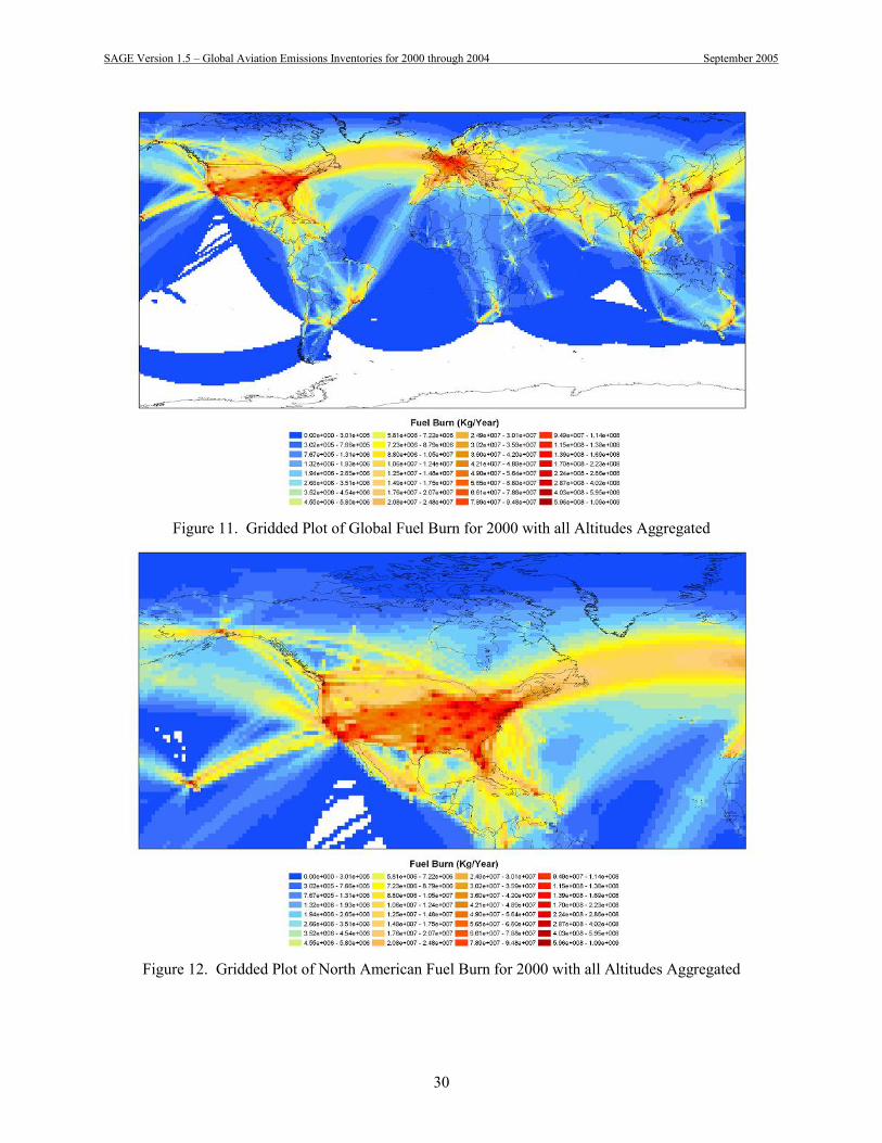
SAGE Version 1.5 – Global Aviation Emissions Inventories for 2000 through 2004 September 2005
30
Figure 11. Gridded Plot of Global Fuel Burn for 2000 with all Altitudes Aggregated
Figure 12. Gridded Plot of North American Fuel Burn for 2000 with all Altitudes Aggregated

SAGE Version 1.5 – Global Aviation Emissions Inventories for 2000 through 2004 September 2005
31
Figure 13. Gridded Plot European Fuel Burn for 2000 with all Altitudes Aggregated
Figure 14. Gridded Plot of Asian Fuel Burn for 2000 with all Altitudes Aggregated

SAGE Version 1.5 – Global Aviation Emissions Inventories for 2000 through 2004 September 2005
32
These gridded plots provide a visual confirmation of the fuel burn hot spots which are predominantly the US, Western Europe, and Eastern Asia. Emissions hot spots are also similarly located as they generally follow fuel burn. Figure 15 shows a distribution of total fuel burn and emissions by 1 km altitude bins for year 2000.
0 5 10 15 20 25 30 35
0 - 1
1- 2
2 -3
3 - 4
4 - 5
5 - 6
6 - 7
7 - 8
8 - 9
9 - 10
10 - 11
11 - 12
13 - 14
Alt
itu
de
Bin
(km
)
.
Percent of Global Total for 2000
HC
CO
NOx
Fuel Burn
Figure 15. Altitude Distribution of Fuel Burn and Emissions for Year 2000
The altitude bins with the highest fuel burn and emissions are between 9 and 12 km (or approximately 29,500 ft and 39,400 ft). This corresponds to the frequent use of these altitudes for en route travel. The relatively high levels of HC and CO in the 0 to 1 km band is due to the higher emissions characteristics for those pollutants at lower power settings (e.g., during taxiing and idle conditions). Similar distributions by longitude and latitude are shown in Figures 16 and 17.

SAGE Version 1.5 – Global Aviation Emissions Inventories for 2000 through 2004 September 2005
33
0.00
0.50
1.00
1.50
2.00
2.50
-179.5 -134.5 -89.5 -44.5 0.5 45.5 90.5 135.5
Midpoint Longitude of each grid cell (degrees)
Pe
rce
nt
of
Glo
ba
l To
tal
Fuel Burn
NOx
CO
HC
Figure 16. Distribution of Fuel Burn and Emissions by Longitude
0
1
2
3
4
5
6
-89.5-44.50.545.5
Midpoint Latitude of each grid cell (degrees)
Per
cen
t o
f G
lob
al T
ota
l
Fuel Burn
NOx
CO
HC
Figure 17. Distribution of Fuel Burn and Emissions by Latitude
As with the altitude distributions, NOx is shown to follow fuel burn more closely than CO or HC in these longitudinal and latitudinal distributions. The three peak sections in Figure 16 roughly correspond to North America, Western Europe, and Eastern Asia. In contrast, the one peak section in Figure 17 roughly

SAGE Version 1.5 – Global Aviation Emissions Inventories for 2000 through 2004 September 2005
34
corresponds to the Northern hemisphere where all of these three regions are located. In combining the longitudinal and latitudinal distributions, the globe was divided into four major quadrants (e.g., North East, North West, etc.) as shown in Figure 18.
0
10
20
30
40
50
60
70
North East North West South East South West
World Quadrant
Pe
rcen
t o
f G
lob
al T
ota
l
Fuel Burn (Tg)
NOx (Tg)
CO (Tg)
HC (Tg)
CO2 (Tg)
H2O (Tg)
SOx (Tg)
Lat: 0 to 90 deg.Long: 0 to -180 deg.
Lat: 0 to 90 deg.Long: 0 to 180 deg.
Lat: 0 to -90 deg.Long: 0 to -180 deg.
Lat: 0 to -90 deg.Long: 0 to 180 deg.
Figure 18. Relative Loadings of Fuel Burn and Emissions by World Quadrant
The much higher fuel burn and emissions levels experienced by the Northern quadrants are, again, mainly due to the flights over North America, Western Europe, and Eastern Asia.

SAGE Version 1.5 – Global Aviation Emissions Inventories for 2000 through 2004 September 2005
35
4 Comparisons to Past Inventories
As SAGE follows upon various previous studies that have been conducted in the past to model global emissions from aircraft, comparisons to these past studies provide reasonability checks as well as wider views of historical trends that could help to better extrapolate to future years. Figures 19 through 23 show comparisons of SAGE global fuel burn and emissions with those from the following past studies [IPCC 1999]:
NASA/Boeing inventories for 1976, 1984, 1992 and 1999 [Baughcuma,b 1996 and Sutkus 2001] ANCAT/EC2 inventories for 1991/92 [Gardner 1998] DLR inventories for 1992 [Schmitt 1997] AERO-MS inventories for 1992 [Pulles 2002]
0
20
40
60
80
100
120
140
160
180
200
1970 1975 1980 1985 1990 1995 2000 2005 2010
Year
Fu
el B
urn
(T
g)
SAGE Version 1.5
NASA/Boeing Scheduled
NASA/Boeing Civil
NASA/Boeing Global
ANCAT/EC2 Civil
ANCAT/EC2 Global
DLR Civil
DLR Global
AERO-MS
Figure 19. Comparison of Fuel Burn from Past Studies

SAGE Version 1.5 – Global Aviation Emissions Inventories for 2000 through 2004 September 2005
36
0
100
200
300
400
500
600
700
1970 1975 1980 1985 1990 1995 2000 2005 2010
Year
CO
2 (T
g)
SAGE Version 1.5
NASA/Boeing Scheduled
NASA/Boeing Civil
NASA/Boeing Global
ANCAT/EC2 Civil
ANCAT/EC2 Global
DLR Civil
DLR Global
AERO-MS
Figure 20. Comparison of CO2 Emissions from Past Studies
0
0.5
1
1.5
2
2.5
3
1970 1975 1980 1985 1990 1995 2000 2005 2010
Year
NO
x (T
g)
SAGE Version 1.5
NASA/Boeing Scheduled
NASA/Boeing Civil
NASA/Boeing Global
ANCAT/EC2 Civil
ANCAT/EC2 Global
DLR Civil
DLR Global
AERO-MS
Figure 21. Comparison of NOx Emissions from Past Studies

SAGE Version 1.5 – Global Aviation Emissions Inventories for 2000 through 2004 September 2005
37
0
0.2
0.4
0.6
0.8
1
1.2
1.4
1.6
1.8
1970 1975 1980 1985 1990 1995 2000 2005 2010
Year
CO
(T
g)
SAGE Version 1.5
NASA/Boeing Scheduled
NASA/Boeing Civil
NASA/Boeing Global
ANCAT/EC2 Civil
ANCAT/EC2 Global
DLR Civil
DLR Global
AERO-MS
Figure 22. Comparison of CO Emissions from Past Studies
0
0.05
0.1
0.15
0.2
0.25
0.3
0.35
0.4
0.45
1970 1975 1980 1985 1990 1995 2000 2005 2010
Year
HC
(T
g)
SAGE Version 1.5
NASA/Boeing Scheduled
NASA/Boeing Civil
NASA/Boeing Global
ANCAT/EC2 Civil
ANCAT/EC2 Global
DLR Civil
DLR Global
AERO-MS
Figure 23. Comparison of HC Emissions from Past Studies
The plots in figures 19 though 21 (fuel burn, CO2, and NOx) generally appear to show noticeable disagreement with the trends established from the past studies. Of all the past studies’ data shown, the most appropriate comparison would be against the NASA/Boeing Scheduled inventories since SAGE Version 1.5 currently only accounts for commercial traffic. The past Civil and Global inventories include

SAGE Version 1.5 – Global Aviation Emissions Inventories for 2000 through 2004 September 2005
38
general aviation and military flights, respectively. Notwithstanding some natural growth in the aviation industry, the approximately 30% difference between the 1999 NASA/Boeing Scheduled inventory totals and the 2000 SAGE totals may in part be explained through differences in trajectory modeling (e.g., Great Circle used by NASA/Boeing versus track distributions used in SAGE) and the inclusion of the effects of unscheduled flights in SAGE (unaccounted in the NASA/Boeing studies). When general aviation and military flights are included in a future version of SAGE, a more appropriate comparison of global totals can be conducted. The CO and HC comparisons in Figures 22 and 23 indicate that SAGE are noticeably different than those suggested by the trends from the past studies. Notwithstanding the differences in distance modeling and unscheduled flights coverage, these types of disagreements with CO and HC are not unexpected since the two pollutants have a greater degree of variability with fuel flow than other pollutants like NOx. Unlike NOx, small changes in fuel flow could result in much larger changes in CO and HC due to the nature of the modeled relationship between fuel flow and EI values [FAAa 2005]. To investigate all of these differences further, the overall emissions indices for each of the pollutants were compared as shown in figures 24 through 26.
0
2
4
6
8
10
12
14
16
1970 1975 1980 1985 1990 1995 2000 2005 2010
Year
NO
x E
I (g
/kg
)
SAGE Version 1.5
NASA/Boeing Scheduled
NASA/Boeing Civil
NASA/Boeing Global
ANCAT/EC2 Civil
ANCAT/EC2 Global
DLR Civil
DLR Global
AERO-MS
Figure 24. Comparison of SAGE Global Average NOx EI Values with Past Studies

SAGE Version 1.5 – Global Aviation Emissions Inventories for 2000 through 2004 September 2005
39
0
5
10
15
20
25
1970 1975 1980 1985 1990 1995 2000 2005 2010
Year
CO
EI
(g/k
g)
SAGE Version 1.5
NASA/Boeing Scheduled
NASA/Boeing Civil
NASA/Boeing Global
ANCAT/EC2 Civil
ANCAT/EC2 Global
DLR Civil
DLR Global
AERO-MS
Figure 25. Comparison of SAGE Global Average CO EI Values with Past Studies
0
1
2
3
4
5
6
7
1970 1975 1980 1985 1990 1995 2000 2005 2010
Year
HC
EI
(g/k
g)
SAGE Version 1.5
NASA/Boeing Scheduled
NASA/Boeing Civil
NASA/Boeing Global
ANCAT/EC2 Civil
ANCAT/EC2 Global
DLR Civil
DLR Global
AERO-MS
Figure 26. Comparison of SAGE Global Average HC EI Values with Past Studies
The NOx EI comparisons in Figure 24 appear to show relatively good agreement between the past studies’ trends and those from SAGE. The difference between the 1999 NASA/Boeing Scheduled EI value and the 2000 SAGE value is about 5%. In contrast, the differences for CO and HC EI values are much greater as shown in figures 25 and 26. Also, the SAGE CO and HC EI values appear to be much less agreeable with the past studies’ trends than for the NOx trends. These results indicate the differences in NOx totals (Figure 21) are less likely due to differences in EI modeling than the aforementioned differences in flight coverage, distance modeling, etc. However, the large differences in CO and HC EI values (figures 25 and 26) support the earlier assertion that the sensitivity of CO and HC EI values to fuel flow could have played a major role in the differences between CO and HC totals shown in figures 22 and

SAGE Version 1.5 – Global Aviation Emissions Inventories for 2000 through 2004 September 2005
40
23. An aircraft-level comparison of a dozen selected aircraft types were conducted as shown in Figure 20.
0.0
2.0
4.0
6.0
8.0
10.0
12.0
14.0
16.0
18.0
A300
-600
A319
A320
A330
-300
A340
-300
B727
-200
B737
-300
/400
/500
B747
-100
/200
/300
B757
-200
B767
-300
BAE
146
Fokk
er 2
8
Fokk
er 1
00
MD
-80
Aircraft
NO
x EI
(g/k
g)
.
1999 NASA/Boeing
SAGE Version 1.5
Figure 27. Comparison of Cruise (> 1 km Altitude above airport field elevation) NOx EI Values by Selected Aircraft Types from SAGE 2000 and NASA/Boeing 1999 Inventories
The aircraft shown in Figure 27 were arbitrarily selected, but they tend to be the most widely flown in the current world fleet. These NOx EI comparisons show reasonable agreement between the two datasets. Although a couple of aircraft types show noticeable differences such as the Fokker 28 (about 33%) and MD-80 (about 24%), most are within 15% difference. The differences in the EIs can be attributed to several factors including differences in the aircraft performance models (i.e., EI is dependent on fuel flow), differences in aircraft and engine mappings, operational changes of the world fleet from 1999 to 2000, and differences in engine assignments. The overall average EI values for the selected aircraft types are 13.2 g/kg for NASA/Boeing and 13.3 g/kg for SAGE Version 1.5. Similar to the comparisons in Figure 24, these values indicate that for the global fleet, the performance module in SAGE appears to produce comparable results to those from the past studies.

SAGE Version 1.5 – Global Aviation Emissions Inventories for 2000 through 2004 September 2005
41
5 Conclusions
SAGE was developed by FAA in large part because there was no up-to-date non-proprietary model thatcould be used to estimate aircraft emissions on a global level. As such, FAA developed SAGE (now atVersion 1.5) from the best publicly available data and methods in order to provide the internationalaviation community with a high-fidelity tool that can be used to analyze various policy, technology, andoperational scenarios. So far, SAGE has been used to develop inventories for 2000-2004. The currentcommitment from FAA is to continue development and validation of SAGE to produce inventories of fuelburn and emissions on a yearly basis.
The flight-level, chord-level, and 4D gridded raw inventories provide high-resolution coverage of fuel burn and emissions as well as various flight parameters (e.g., aircraft performance data, flight schedule data, etc.). These inventories provide the potential for the development of numerous processed inventories to analyze various aspects of global aviation’s fuel burn and emissions including temporal trend analyses, event investigations (e.g., 9/11), and comparison assessments. The typical processed inventories presented in Sections 3.1 through 3.3 exemplify the uses of the data including the derivation of calculated metrics (e.g., fuel burn per distance, NOx EI values, etc.) that can be used to assess the effects of policy, technology, and operational changes to global aviation. Since the raw inventories were too large to include in this report, several processed inventories are included in the appendices in order to simulate the details and comprehensiveness of the raw inventories. In providing this data, a balance was chosen to provide as much useful data as possible but within reasonable limits to keep the data size manageable.
In general, most of the processed inventories presented in Sections 3.1 through 3.3 are intuitive. That is, trends, relative comparisons, et cetera appear to agree with the current understanding and state of the aviation industry. The comparison against previous studies showed noticeable differences in the overall, global fuel burn and emissions estimates. The SAGE fuel burn and NOx results appeared to be approximately 30% greater than that expected from the trends exhibited from the previous studies. Since the comparison of NOx EI values on both global and aircraft levels showed good agreement, the performance model in SAGE appears to be of comparable quality to those used in past studies. Therefore, most of the differences in the overall fuel burn and NOx estimates are likely to be due to differences in trajectory modeling, unscheduled flight coverage, etc.
The development of SAGE Version 1.5 and the inventories for 2000 through 2004 are based on the goal to provide FAA, and indirectly the international aviation community, with a standard and open model that can be used to generate high-fidelity global inventories of fuel burn and emissions in helping to answer various policy, technology, and operational questions. FAA is committed to supporting the continued development and validation of SAGE in producing yearly inventories of fuel burn and emissions. Therefore, the data and methods within SAGE and the inventories generated thereof will stay relevant year after year.

SAGE Version 1.5 – Global Aviation Emissions Inventories for 2000 through 2004 September 2005
42
References
Baughcuma, S.L., T.G. Tritz, S.C. Henderson, and D.C. Pickett. “Scheduled Civil Aircraft Emission Inventories for 1992: Database Development and Analysis.” NASA CR 4700. April 1996.
Baughcumb, S. L., S. C. Henderson, and T. G. Tritz. “Scheduled Civil Aircraft Emission Inventories for 1976 and 1984: Database Development and Analysis.” NASA CR-4722. 1996.
Federal Aviation Administration (FAAa). “System for assessing Aviation’s Global Emissions (SAGE), Version 1.5, Technical Manual.” FAA, Office of Environment and Energy. FAA-AEE-2005-01. September 2005.
Federal Aviation Administration (FAAb). “System for assessing Aviation’s Global Emissions (SAGE), Version 1.5, Validation Assessment, Model Assumptions and Uncertainties.” FAA, Office of Environment and Energy. FAA-AEE-2005-03. September 2005.
Gardner, R. “Global Aircraft Emissions Inventories for 1991/92 and 2015, Report by the ECAC/ANCAT and ED Working Group.” Editor: R. M. Gardner. EUR18179. 1998.
Intergovernmental Panel on Climate Change (IPCC). “Revised 1996 IPCC Guidelines for National Greenhouse Gas Inventories, Reference Manual (Volume 3).” http://www.ipcc-nggip.iges.or.jp/public/gl/invs6.htm. 1997.
Intergovernmental Panel on Climate Change (IPCC). “Aviation and the Global Atmosphere.” A Special Report of IPCC Working Groups I and II. Edited by J.E. Penner, D.H. Lister, D.J. Griggs, D.J. Dokken, and M. McFarland. Cambridge University Press. 1999.
Pulles, J.W. “Aviation Emissions and Evaluation of Reduction Options (AERO), Main Report.” Ministry of Transport, Public Works and Watermanagement, Directorate-General of Civil Aviation, the Hague. ISBN 90-369-1792-1. July 2002.
Schmitt, A., B. Brunner. “Emissions from Aviation and their Development over Time. In Final Report on the BMBF Verbundprogramm, Schadstoff in der Luftfahrt. DLR-Mitteilung 97-04, Deutches Centrum Fuer Luft- and Raumfahrt. 1997.
Sutkus Jr., Donald J., Steven L. Baughcum, and Douglas P. DuBois. “Scheduled Civil Aircraft Emission Inventories for 1999: Database Development and Analysis.” National Aeronatics and Space Administration (NASA) Glenn Research Center, Contract NAS1-20341. NASA/CR-2001-211216. October 2001.
United Nations Environment Programme (UNEP)/World Meteorological Organization (WMO). Article 4 of the Framework Convention on Climate Change published by the UNEP/WMO Information Unit on Climate Change (also identified in Article 12). See <http://unfccc.int>. 2000.