Safe Haven CDS Premiums∗

Sven Klingler†

David Lando‡

July 8, 2017

Abstract

Credit Default Swaps can be used to lower capital requirements of dealer banks whoenter into uncollateralized derivatives positions with sovereigns. We show in a modelthat the regulatory incentive to obtain capital relief makes CDS contracts valuableto dealer banks and empirically that, consistent with the use of CDS for regulatorypurposes, there is a disconnect between changes in bond yield spreads and in CDSpremiums especially for safe sovereigns. Additional empirical tests related to volumesof contracts outstanding, effects of regulatory proxies, and the corporate bond andCDS markets support that CDS contracts are used for capital relief.

CDS premiums, capital charges, CVA, CDS-bond basis; JEL: F34, G12, G15

∗We are grateful to Patrick Augustin, Nicolae Garleanu, Jesper Lund, Allan Mortensen, Martin Oehmke,Lasse Pedersen, Stephen Schaefer, Martin Scheicher, Suresh Sundaresan, Matti Suominen, Davide Tomio,Guillaume Vuillemey, and participants in Advanced Topics in Asset Pricing at Columbia University, AnnualMeeting of the German Finance Association (2014), Arne Ryde Workshop, Aarhus Business School, BancoPortugal, EPFL, ESSEC, European Finance Association (2015), The Federal Reserve Bank of New York,Imperial College, and American Finance Association (2016) for helpful comments. Pia Mølgaard assisted uswith the corporate bond and CDS data. Support from the Center for Financial Frictions (FRIC), grant no.DNRF102, is gratefully acknowledged.†Department of Finance and Center for Financial Frictions (FRIC). Copenhagen Business School, Solbjerg

Plads 3, DK-2000 Frederiksberg, Denmark. E-mail: sk.fi@cbs.dk‡Department of Finance and Center for Financial Frictions (FRIC). Copenhagen Business School, Solbjerg

Plads 3, DK-2000 Frederiksberg, Denmark. E-mail: dl.fi@cbs.dk

1 Introduction

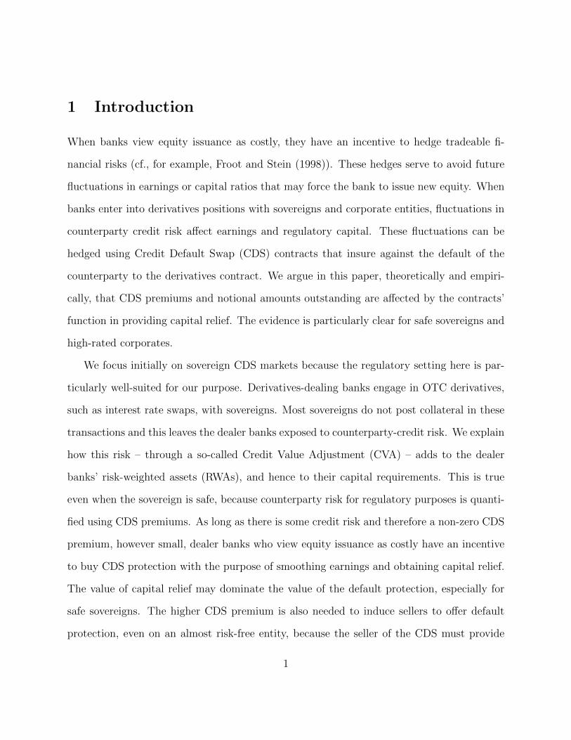
When banks view equity issuance as costly, they have an incentive to hedge tradeable fi-

nancial risks (cf., for example, Froot and Stein (1998)). These hedges serve to avoid future

fluctuations in earnings or capital ratios that may force the bank to issue new equity. When

banks enter into derivatives positions with sovereigns and corporate entities, fluctuations in

counterparty credit risk affect earnings and regulatory capital. These fluctuations can be

hedged using Credit Default Swap (CDS) contracts that insure against the default of the

counterparty to the derivatives contract. We argue in this paper, theoretically and empiri-

cally, that CDS premiums and notional amounts outstanding are affected by the contracts’

function in providing capital relief. The evidence is particularly clear for safe sovereigns and

high-rated corporates.

We focus initially on sovereign CDS markets because the regulatory setting here is par-

ticularly well-suited for our purpose. Derivatives-dealing banks engage in OTC derivatives,

such as interest rate swaps, with sovereigns. Most sovereigns do not post collateral in these

transactions and this leaves the dealer banks exposed to counterparty-credit risk. We explain

how this risk – through a so-called Credit Value Adjustment (CVA) – adds to the dealer

banks’ risk-weighted assets (RWAs), and hence to their capital requirements. This is true

even when the sovereign is safe, because counterparty risk for regulatory purposes is quanti-

fied using CDS premiums. As long as there is some credit risk and therefore a non-zero CDS

premium, however small, dealer banks who view equity issuance as costly have an incentive

to buy CDS protection with the purpose of smoothing earnings and obtaining capital relief.

The value of capital relief may dominate the value of the default protection, especially for

safe sovereigns. The higher CDS premium is also needed to induce sellers to offer default

protection, even on an almost risk-free entity, because the seller of the CDS must provide

1

initial margin, and there is an opportunity cost of providing this margin. The end result is

an equilibrium in which the CDS premium is significantly higher than what can be explained

by credit risk alone.

We explain the mechanism in a simple one-period model with two agents: The first

agent is a derivatives dealing bank who holds a legacy position in an interest rate swap

with a sovereign which adds to the bank’s capital requirement. The dealer bank can buy

CDS protection from the second agent who is an end user of derivatives with no previous

exposure to the sovereign. The end user allocates his risky investment between the risky

asset and selling CDS protection. Our model offers quantitative guidance as to how CDS

premiums depend on margin requirements for the seller and the buyer of CDS protection,

capital requirements of the dealer bank and limits on leveraged investment in the risky asset.

We present a variety of empirical tests to support our hypothesis that CDS contracts serve

a regulatory purpose and that this is particularly visible for safe reference entities. First, we

look at connections between derivatives positions of banks with sovereign counterparties and

the net notional amounts of sovereign CDS outstanding. As a first reality check, we confirm

that derivatives dealers are net buyers of sovereign CDS, and that the level and volatility of

CDS premiums can justify purchasing protection on safe sovereigns for regulatory purposes.

Our estimates of the CDS notional amount that can potentially be explained by the Basel

III CVA capital charges can account for more than 50% of the total sovereign CDS volume

outstanding, a number that is in line with estimates found in industry research letters.

Passing these reality checks, we turn to information on bank derivative exposures toward

sovereigns from EBA bank stress tests, which we use as a proxy for banks’ expected exposure

toward sovereigns. In line with our hypothesis, we find a significant relationship between

these exposures and CDS amounts outstanding.

2

Second, changes in bond yield spreads and changes in CDS premiums are almost unrelated

for safe sovereigns. A central prediction of our model is that the regulatory component of

CDS premiums is relatively larger for safe sovereigns than for less safe sovereigns. Figure

1 shows that regressing changes in bond yields on changes in the riskless rate (proxied by

overnight swap rates) and changes in CDS premiums reveals a clear pattern in which the

CDS premium explains a larger part of bond yields the riskier the sovereign becomes. For

Germany, Japan, and the United States CDS premiums are not a significant explanatory

variable for bond yields. For Great Britain the CDS premium is significant, but only at

a 10% level. For the three risky European sovereigns in our sample (Italy, Portugal, and

Spain), the regression coefficient on the CDS premium is close to one. We perform robustness

checks to rule out other potential explanations for this disconnect, such as the convenience

benefits of safe assets and the cheapest-to-deliver option embedded in sovereign CDS. We

also extend our “clean” sample of 10 sovereigns to a larger cross-section and show that our

results hold for that extended cross-section as well.

Third, we test whether proxies for the constraints imposed by capital requirements help

explaining CDS premiums. We find that for the risky sovereigns, Italy, Portugal, and Spain,

CDS premiums are mainly driven by credit risk. For the low-risk sovereigns Austria, Finland,

and France, both credit and our regulatory capital proxies, have strong explanatory power

for CDS premiums. Therefore, our theory does not only apply to safe-haven sovereigns but

extends to entities with a low credit risk. For the safe-haven sovereigns Germany, UK, Japan,

and the US, we find that regulatory proxies are significant and can explain up to 29% of the

variation in CDS premiums.

Finally, evidence from corporate bonds suggests that the regulatory effects also carry over

to safe corporate issuers. Using data for corporates offer two advantages over sovereigns.

3

First, corporate CDS contracts have been actively traded prior to the financial crisis, and

we can therefore test effects of regulatory changes. Second, we can distinguish between

financial firms and non-financial firms. Non-financial firms typically do not post collateral

in their derivatives transactions and we would therefore expect to see a similar pattern of

falling correlation between CDS premiums and bond yield spreads as credit quality increases.

Financial firms are more likely to collateralize their derivatives positions and we would

therefore expect a stronger relationship between CDS premiums and bond yield spreads for

these issuers. Two tests confirm our hypothesis. First, we again find a weaker link between

CDS premiums and bond yields for safe corporate issuers than for risky corporate issuers.

Second, we find that the link between CDS premiums and bond yields for safe corporates

breaks down after the financial crisis and more so for corporate issuers than for financial

issuers.

2 Related Literature

Figure 2 illustrates the disconnect between CDS premiums and bond yield spreads for Ger-

many and the much closer connection for France and Italy. The observed patterns could not

occur in a frictionless market where an increase in the CDS premium would also increase the

corresponding bond yield. More precisely, the CDS premium and bond yield spread should

be equal due to an arbitrage relationship. Hence, our work is related to the growing litera-

ture on the limits of arbitrage, as introduced by Shleifer and Vishny (1997) and studied by

Gromb and Vayanos (2002) for the case when arbitrageurs need to collateralize their posi-

tions. Gromb and Vayanos (2010) survey the literature on limits of arbitrage and summarize

the basic idea in these models. An exogenous demand shock for a certain asset occurs to out-

4

side investors and arbitrageurs, who both are utility-maximizing and constrained, and take

advantage of the shock by providing the asset. We contribute to this literature by providing

a parsimonious model in the spirit of Garleanu and Pedersen (2011), which incorporates the

supply and demand side, as well as the explicit financial frictions that drive the potential

mispricing.

Yorulmazer (2013) is an early contribution arguing that capital relief is an important

motive for banks to buy CDS protection. His main concern is how this may lead to in-

creased systemic risk in the banking system. We provide solutions for CDS premiums that

incorporate the exact institutional features of CDS trading and capital relief, and we provide

empirical support in several dimensions.

The difference between the CDS premium and the yield spread is commonly referred to

as the CDS-bond basis and there is a large strand of literature aiming to explain this basis.

Empirically, the CDS-bond basis has been studied for corporate issuers by, among others,

Blanco, Brennan, and Marsh (2005), Longstaff, Mithal, and Neis (2005), and Bai and Collin-

Dufresne (2013). O’Kane (2012), Gyntelberg, Hordahl, Ters, and Urban (2013), and Fontana

and Scheicher (2014) analyze the CDS-bond basis for European sovereigns. Our empirical

analysis complements this strand of literature by showing that for safe governments, changes

in CDS premiums and yield spreads are virtually unrelated.

Garleanu and Pedersen (2011) argue that the corporate CDS-bond basis is, to a large

extent, driven by different margin requirements for bonds and CDS. Moreover, He, Kelly,

and Manela (2016) show that there is a significant link between the returns of corporate

CDS and dealer banks’ balance sheet constraints. In line with these papers, we find that

dealer banks’ balance sheet constraints are relevant for sovereign CDS. We contribute to

this literature by adding an explanation for the demand for CDS on safe sovereigns, which,

5

according to our hypothesis, comes from regulatory frictions.

The drivers of sovereign CDS premiums have been widely studied. Pan and Singleton

(2008) and Longstaff, Pan, Pedersen, and Singleton (2011) explain them by global investors’

risk appetite, Ang and Longstaff (2013) suggest systemic risk as one potential driver, and

Anton, Mayordomo, and Rodriguez-Moreno (2015) suggest that buying pressure of CDS

dealers plays a role. In addition, our theory helps explaining changes in the amounts of CDS

outstanding, which have been studied by Oehmke and Zawadowski (2016) for corporate CDS

and by Augustin, Sokolovski, Subrahmanyam, and Tomio (2016) for sovereigns. Augustin,

Subrahmanyam, Tang, and Wang (2014) provide an extensive survey on sovereign CDS

premiums.

Chernov, Schmid, and Schneider (2015) model default risk premiums of the U.S. govern-

ment, and CDS premiums on U.S. government debt are also touched upon in Brown and

Pennacchi (2015), who argue that there may well be a credit risk element in U.S. Treasuries

arising from underfunding of pension plans, and that U.S. CDS premiums reflect default risk.

We agree that there may well be default-risk premiums for safe-sovereign CDS contracts, but

we argue that the regulatory incentive to hold these contracts dominates in their pricing.

Illiquidity premiums in CDS have been studied in Bongaerts, de Jong, and Driessen

(2011) and Junge and Trolle (2014), but these papers do not deal with sovereign CDS which,

judging from volumes outstanding and trading activity, are by far the most liquid contracts.

3 Regulation and Sovereign CDS Demand

We first highlight the essential features of regulation of uncollateralized derivatives positions

for banks that motivate our model and our empirical findings. A significant part of large

6

dealer banks’ exposure to sovereign entities comes from interest rate swaps and other over-

the-counter (OTC) derivative positions. Unlike financial entities, most sovereigns do not post

collateral in OTC derivatives positions and this leaves dealer banks exposed to counterparty

credit risk. The current regulatory regime, referred to in short as Basel III (see Basel

Committee on Banking Supervision, 2011), contains a charge related to this counterparty

credit risk. While the risk of losses related to outright default of a derivatives counterparty

had been dealt with in previous Basel accords, this new capital charge was motivated by

the significant mark-to-market losses of derivatives positions that arose from deteriorating

credit quality (but not outright default) of counterparties during the financial crisis1.

A bank will suffer mark-to-market losses if an OTC exposure has positive value to the

bank and the credit quality of the counterparty deteriorates. In technical terms, a dete-

riorating credit quality will lead to an adjustment in the Credit Value Adjustment (CVA)

of the bank’s position. The CVA measures the difference between the value of the OTC

exposure if held against a default-free counterparty versus a risky counterparty. When this

difference increases, it implies a loss to the bank. Basel III imposes an addition to the bank’s

Risk Weighted Assets (RWAs), and therefore ultimately to its capital requirement, related

to the risk of changes in the CVA. Importantly, the default risk of the counterparty that goes

into the CVA calculation is measured using CDS premiums. This means that regardless of

how safe the counterparty is, there is a capital charge as long as the CDS premium on the

counterparty is not constant and strictly positive.

Basel III gives banks the option to avoid this addition to RWAs by purchasing CDS on

the counterparty. Hence, this regulatory framework gives dealer banks an incentive to buy

1According to a Basel Committee 2011 press release http://www.bis.org/press/p110601.htm, duringthe financial crisis, ”roughly two-thirds of losses attributed to counterparty credit risk were due to CVAlosses and only about one-third were due to actual defaults”.

7

sovereign CDS instead of merely acting as net sellers of CDS contracts, which is common in

most other markets. In line with this argument, Figure 3 shows that from 2010 on, after the

announcement of Basel III, derivatives dealers are indeed net buyers of sovereign CDS. This

is in contrats with the corporate CDS market, wehere deaer banks are typically short CDS

contracts. 2 The notional amount of CDS that the bank needs to buy in order to obtain full

capital relief is equal to so-called expected exposure (EE) arising from the OTC position.

If the position is left unhedged, it will lead to an increase in RWAs that is proportional

to EE and therefore a corresponding increase in the bank’s capital requirement equal to a

fraction of EE. It is the trade-off between the cost of buying protection and the benefit of

obtaining capital relief that is fundamental to our model in the next section. More details

on the computaion of expected exposures and CVAs can be found in Appendix C.

4 The Model

We set up a simple one-period model that focuses on determining the CDS premium. In this

model, a bank has an incentive to purchase CDS protection on an entity to obtain capital

relief. An end user can earn the CDS premium by selling CDS to the bank, but needs trading

capital to do so.

4.1 The Assets

There are three different assets in the economy. First, there is a risky asset with price

normalized to one, and normally-distributed time-1 payoff r ∼ N (1 + µ, σ2). We want to

2Unfortunately, there is no information for the buyers and sellers of individual sovereigns available. Hence,we cannot claim that the variation of the notional amount of sovereign CDS bought by dealers can only betraced to financial regulation. It is also possible that, especially during the European debt crisis, the endusers’ demand for CDS on risky sovereigns increased.

8

focus on the CDS premium and therefore take µ and σ2 as exogenously given constants.

The risky asset has a margin requirement m for both buying and short-selling the asset.

Hence, one unit of wealth can at most support a long or short position of 1/m in the risky

asset. From a regulatory perspective, the risky asset contributes to the risk-weighted assets

of the bank. We choose for simplicity to let m also denote the contribution to the capital

requirement for the bank associated with holding one unit of the risky asset. Second, a

risk-free asset which pays off 1 + r for each unit invested in it at time 0. We assume that

the risk-free asset is in perfectly elastic supply and that r is an exogenously given constant.

Third, a CDS contract on an entity which is not part of the model and can be thought of as

a safe sovereign. The CDS premium s is the main focus of our model and will be determined

in equilibrium. We denote by s the random payoff on the CDS as seen from the protection

buyer:

s :=

−s, with probability 1− p

LGD, with probability p

and hence the expected pay-off as seen from the protection buyer is

s := pLGD− (1− p)s.

The initial margin for buying and selling the CDS is n+ and n− respectively. The notional

amount of CDS outstanding is determined in equilibrium. The quantities s, n+, and n− are

all per unit of insured notional, so the relevant dollar amounts are obtained by multiplying

the numbers with the notional amount on the CDS contract. We refer to a long position in

the CDS as representing a purchase of insurance. If, for example, s = 45 bps, a purchase

9

of insurance of 1 dollars of notional, requires a payment of 0.0045 dollars at the end of the

period if there is no default, and leads to a positive cash flow equal to LGD = 0.6 if there is

a default3.

4.2 The Agents and Their Constraints

There are two different agents, a derivatives-dealing bank B and an end user of derivatives

E. Agent i′s wealth at time 1 is then given as:

W i1 = W i

0(1 + r) + g(r − r) + gs,

where g ∈ {b, e} denotes the dollar amount of wealth invested in the risky asset for each agent

type, and g ∈ {b, e} denotes the notional amount insured by the CDS for each agent type.

So, for example, b refers to the dollar amount on which the bank has bought protection (if b

is positive) or sold protection (if b is negative). We assume that agents solve a mean-variance

problem in which the optimization objective takes the form

maxg,g

[g(µ− r) + gs− 1

2(σg)2 − 1

2v(s)g2

],

where v(s) = (p − p2)[LGD2 + 2sLGD] is an approximation of the variance of the CDS

payoff.4 We have chosen the risk aversion parameter for both agents to be equal to one.

There will only be a supply of CDS from the end user when the expected return on buying

3According to Moody’s Investors Service (2011), the average recovery rates for sovereigns measured astrading price after 30 days divided by principal for defaults in the period is 31% (value weighted) and 53%(issuer weighted).

4The only difference between v(s) and the variance of the CDS payoff is a term of the form (p−p2)s2 whichfor the range of CDS premiums we consider is at least an order of magnitude smaller than the dominatingterm.

10

CDS protection is negative, i.e. s < 0, so that there is a compensation for the risk of selling

protection, and this will be the case in equilibrium.

The agents’ constraints involve capital requirements of the bank and funding requirements

of the end user. Recall that the amount of wealth required to establish a position g in the

risky asset is the same for long and short positions and given by m|g|. We refer to m|g|

as the margin requirement and to the wealth constraint due to margin requirements as the

margin constraint. The margin requirement for establishing a long position g > 0 in the

CDS (buying protection) is given by n+g and by n−|g| for establishing a short position g < 0

(selling protection). We think of the agent as having to deposit the amount of cash in a

margin account where it earns the risk-free rate r.

The bank and the end user differ in their margin constraints. The end user’s constraint

is given as:

me+ n−|e| ≤ WE0 . (1)

Equation (1) can be interpreted as follows. The end user can invest a maximum amount of

WE0

min the risky asset. This would rule out taking a position in the CDS contract because

any non-zero position in the CDS contract reduces the degree to which the agent can make

a levered investment in the risky asset. In equilibrium, the end user will only take long

positions in the risky asset. Further, the end user will only consider selling the CDS in order

to earn the CDS premium if it offers a positive expected return to do so.

The bank faces a different constraint arising from regulatory capital requirements. We

assume that the bank has an interest rate swap with the reference entity of the CDS out-

standing.5 This position adds to the risk-weighted assets of the bank and reduces the bank’s

5To keep the focus of our model on the equilibrium CDS premium, we abstract from modelling theinteraction between the bank and the safe sovereign.

11

ability to lever its risky asset or take positions in the CDS market. As explained in Section

3, the contribution to risk-weighted assets is proportional to the expected exposure EE of

the interest rate swap. The proportionality factor κ depends on the risk that the credit

quality of the counterparty deteriorates over the lifetime of the interest rate swap. This

risk is measured through the level and the volatility of the CDS premium. The bank can

free up capital by purchasing CDS, and a CDS with notional amount equal to EE removes

the capital charge entirely. This frees up capital for investing in the risky asset, and this

is the reason why the bank is willing to enter into a CDS which has a negative expected

excess return. The bank does not gain any capital relief from buying protection on a larger

notional than EE. Rather than representing this as a kink in the margin constraint, we add

the constraint b ≤ EE to our optimization problem. Therefore, the bank’s margin constraint

can be written as:

mb+ n+b+ κ(EE − b) ≤ WB0

b ≤ EE. (2)

In equilibrium, the bank takes a long position in the risky asset and has a non-negative

position in the CDS. This is because the only other agent involved in the CDS market is the

end user who, in equilibrium, sells CDS.

4.3 Equilibrium

In the market described above, equilibrium is defined by a premium s on the CDS contract

and positions in the CDS contracts such that

12

(i) Agents maximize the mean-variance utility

[g(µ− r) + gs− 1

2(σg)2 − 1

2v(s)g2

]

subject to the constraints (1) and (2) respectively.

(ii) The CDS market clears:

b+ e = 0. (3)

Before stating our main result, we introduce the following three parameter restrictions

that we label “regularity conditions:“

1

mmax

(WE

0 ,WB0 − n+EE

)>µ− rσ2

(4)

κ > n+ (5)

min

(WE

0

n−,WB

0

κ

)> EE (6)

Condition (4) ensures that the agents are margin-constrained and conditions (5) and (6)

ensure that the bank has capital for investing in the risky asset and can potentially benefit

from purchasing the CDS. Under these regularity conditions we can now state our main

result.

Proposition 1. Assume that the regularity conditions are satisfied and define

sb :=1

(1− p)(1 + 2R)

(κ− n+

m

(µ− r − σ2

m(WB

0 − EEn+)

)+ pLGD

)− RLGD

(1 + 2R)(7)

sef :=1

(1− p)(1− 2R)

(n−

m

(µ− r − σ2

m(WE

0 − n−EE)

)+ pLGD

)+RLGD

1− 2R, (8)

13

where R := pEELGD.

If sef ≤ sb, then sef is the unique equilibrium CDS premium and in this equilibrium, the

bank buys full protection on its entire expected exposure b = EE from the end user.

The proof of Proposition 1 can be found in Appendix B. We also characterize the case

in which the bank buys partial protection in more detail in the appendix.

Numerical Example

In Figure 4 we illustrate the model by plotting, for a set of parameters, the supply −e and

demand b for CDS as a function of the CDS premium. With our choice of parameters,

described below, the end user starts selling CDS for s > 84 basis points and would in fact

be buying CDS for s < 9 basis points. The bank is willing to buy CDS up to a value of the

premium equal to 192 bps. The CDS market clears for a CDS premium of s = 105 basis

points.

Our motivation for the choice of parameters is as follows: We set the expected excess

return to µ − r = 0.055. The standard deviation of the risky asset is given as σ = 0.2,

which is approximately the long-term mean of the S&P 500 implied volatility index VIX.

The initial wealth of bank and end user are set to WB0 = WE

0 = 0.2 to obtain binding margin

constraints for both agents. Trading the risky asset requires an initial margin of m = 0.2

and this is also the addition to the capital requirement of the bank per unit of additional

risky asset. We follow Garleanu and Pedersen (2011) and assume a margin requirement of

5% for low risk CDS entities. Fourth, the default probability of the sovereign is p = 0.75%

with LGD = 0.6, which in a risk neutral world would correspond to a CDS premium of 45

basis points. The bank either faces an addition to its risk-weighted assets of κEE = 0.06

with κ = 0.15 and EE = 0.4 or buys CDS to free regulatory capital. Our choice of κ is is

14

based on the methods explained in Appendix C. EE is chosen as a large number relative to

the bank’s and end user’s wealth for illustrative purposes.

Model Implications

Focusing first on the case where the bank buys full protection, the solution for the CDS

premium given in Equation (8) has the following implications. First, an increasing expected

exposure (EE) on the bank’s swap position, which, in equilibrium, increases the demand for

CDS protection, increases the premium. Second, a higher margin requirement for selling

the CDS (i.e. a higher n−), increases the CDS premium. However, it is important to

keep in mind that the expression for the equilibrium CDS premium only holds if se < sb.

Therefore, if margin requirements become too high, this may cause a decreasing demand

for CDS protection by the bank and therefore a lower CDS premium. Third, a capital-

constrained bank is willing to pay an additional premium for CDS protection. Fourth, a

higher excess return implies a higher CDS premium. Finally, assuming that the expected

excess return is fixed, Equation (8) implies that a higher volatility of the risky asset decreases

the CDS premium. This is because investments in the risky asset become less attractive as

the volatility increases when expected excess return is fixed.

Our model shows that in the limit as the default probability of the underlying sovereign

goes to zero, the CDS premium approaches a strictly positive level. Hence, in the limit as

credit risk becomes small, only the regulatory incentive to buy CDS matters. In a world

where the CDS premium and its volatility were zero, and banks had no exposures to hedge,

a zero CDS premium would be an equilibrium too. But an infinitesimal disturbance away

from zero brings us to our equilibrium premium. One could worry that once we are away

from zero, a ”doom loop” (as mentioned in Murphy (2012)) would be created in which higher

15

CDS premiums lead to higher regulatory demand which in turn increases CDS premiums,

thus creating an upward spiral. Fortunately, our model shows that as long as the Expected

Exposure is fixed and the bank is constrained, a higher capital charge does not change the

fact that the bank demands a notional equal to its expected exposure, and therefore no

”doom loop” occurs. However, the derivative of our equilibrium CDS premium with respect

to the default probability of the underlying is higher than in a model where there is no capital

relief associated with buying CDS. The total effect as the credit risk moves away from zero

is therefore more similar to an addition to the default risk premium which is proportional to

the actual default risk.

5 Empirical Evidence

We now turn to our empirical analysis which falls into four broad categories: First, we

investigate whether the regulatory relief per unit of CDS protection bought gives institutions

an incentive to buy protection, and we investigate the volumes of CDS outstanding compared

to the aggregate derivatives exposures of banks to sovereigns. Next, we investigate the

covariation between CDS premiums and sovereign bond spreads. The regulatory incentive

to buy CDS protection should lead to a smaller correlation between CDS premiums and

bond yields for safe sovereigns, where the regulatory component can be large compared to

the credit risk component. Third, we test whether different proxies for bank’s incentives

to hedge (capital constraints, increases in the size and risk of expected exposures) have an

effect on CDS premiums. Finally, we investigate whether the pattern of smaller correlation

between CDS premiums and yield spreads for safe entities can also be found in U.S. corporate

bond markets, whether the pattern is different for financial firms and non-financial firms,

16

and whether the pattern changes before and after the crisis.

5.1 Linking CDS Volume to CVA Hedging

According to several industry research notes, a large fraction of the outstanding sovereign

CDS volume can be a consequence of financial regulation. For example, the fraction is

estimated to be 25% in Carver (2011) and up to 50% in ICMA (2011). In Appendix D, we

provide more anecdotal evidence to support our claim that derivatives dealers use sovereign

CDS to hedge CVA risk as well as more detailed sample calculations. In this section, we

focus on sample calculations and statistical tests.

To justify the use of sovereign CDS for CVA hedging, we need to make sure that the

amount of capital relief per unit of CDS notional bought, κ(s) as defined in Equation (38)

in Appendix C, is large enough to outweigh the margin costs associated with buying CDS

contracts. Note that κ(s) can be computed from historical CDS data. We use CDS premi-

ums for 10 different sovereigns, and our calculations of κ(s) show that it is typically optimal

for banks to hedge their entire CVA VaR using CDS contracts. Hence these sample calcula-

tions suggest a connection between the volume of bank derivatives positions with sovereign

counterparties and the amount of CDS contracts outstanding.

Data

We collect data on OTC derivatives outstanding for 28 different sovereigns from the 2013

EBA stress tests and 28 countries from the 2015 stress tests. The data refer to all OTC

derivatives that a sovereign, or a government-sponsored entity, which was part of the EBA

stress test,6 has with derivatives dealing banks. The net notional of CDS outstanding is

6Stress tests were conducted on banks in all European countries, including Great Britain. However,volumes for derivatives-dealing banks in Switzerland and the United States are not included in the notional

17

obtained from DTCC, CDS premiums are obtained from Markit, and the countries’ debt

outstanding is obtained from countryeconomy.com. We explain these data (as well as all

other data in this paper) in more detail in Appendix A.

CVA and Risk Charges Associated with Derivatives

We initially focus on the 10 sovereigns which we consider our main sample and for which

we later run additional tests. In column 1 and 2 of Table 1, we report the notional value

and the fair value of all derivatives for these 10 sovereigns that have positive fair value for

banks. The fair value of all derivatives with positive value gives an indication of how deep

the derivatives are in-the-money. While netting of a banks’ exposure with a sovereign might

imply a smaller expected exposure than the amount indicated by the fair value, there are

other reasons why the expected exposure may be larger. First, the current fair value of a

derivative nets out positive and negative values that the derivative may have in the future,

whereas the calculation of expected exposure is only based on values in future states in which

the derivative has positive value. Second, the EBA data do not account for OTC exposures

that non-European banks have with these sovereigns. Third, the fair value does not account

for the option-like feature of Expected Exposure discussed in Appendix C.

Because banks would need to buy CDS protection on a notional amount equal to the

expected exposure to hedge their OTC derivatives exposure toward sovereigns, the fair value

of the outstanding derivatives with sovereign counterparties gives an indication of whether

the order of magnitude of such positions is comparable to the amounts of CDS outstanding7.

Column 4 of Table 1 reports the amount of sovereign CDS outstanding for the respective

amounts. Hence, all exposures are underestimated because some derivatives dealers are missing.7An alternative method for estimating expected exposures of banks to Germany based on more specific

data on swap positions of the German federal government’s is available for Germany is available upon request.

18

countries. As we can see from the table, in all cases except for the US, the notional amounts of

CDS outstanding are of the same order of magnitude as the fair value of derivatives positions

with positive value. We test the relationship between CDS net notionals outstanding and

sovereigns’ derivatives positions on a larger cross-section of countries below.

Column 9 (furthest to the right) of Table 1 shows the amount of capital relief κ(s) that

one unit of sovereign CDS purchase will provide. Columns 5-8 provide the necessary input

to calculate κ(s). The steps are explained in detail in Appendix C. As we can see, the value

ranges from lowest value of κ(s) = 0.052 for the U.S. to the highest value of κ(s) = 0.821 for

Portugal. In Proposition 1, κ(s) is written as κ, and we note that the regularity condition

κ > n+ is satisfied for all countries if we assume n+ = 0.05. Note that it is likely that the

margin requirement for buying CDS – especially on safe sovereigns – is in fact smaller than

0.05 because the margin would easily exceed the present value of the CDS contract even if

the premium dropped to zero. Therefore we can justify the purchase of a CDS as providing

capital relief in all cases.

Testing the Link Between CDS Volumes and CVA Risk

After having established that our estimate of CVA hedging need is of the same order of

magnitude as the sovereign CDS market for our sample of 10 sovereigns, we next conduct

a formal test of whether there is a link between CDS volumes outstanding and sovereigns’

derivatives exposures to banks on a larger sample. To that end, we expand the sample to

include all sovereigns that have derivatives positions with a positive fair value for European

and UK banks. We also add the results from the December 2015 stress tests. Panel (a) of

Figure 5 shows a scatter plot of CDS volumes outstanding (measured as the net notional

outstanding) against the fair value of all derivatives with positive value for reporting banks

19

(both on a logarithmic scale). As we can see from the figure, there is a strong positive

relationship between the two numbers; In line with our hypothesis that financial regulation

drives the demand for sovereign CDS, we find that there are more CDS outstanding on

sovereigns with more derivatives contracts outstanding. The only large outlier is China,

where the CDS net notional outstanding is significantly larger than the fair value of banks’

derivatives positions.

To test the significance of the relationship between sovereign CDS outstanding and banks’

derivatives exposures, we next run cross-sectional regressions of the the following form:

log(CDSi,t) = α + β log(Derivativesi,t) + Controlsi,t + εi,t, (9)

where Derivativesi,t is the fair value of all derivatives with positive fair value to banks.

Table 2 shows the results of this test. In Panel (1), we run regression (9) without addi-

tional controls. We add a dummy variable for the level and the slope coefficient in Panel

(2). The dummy varable is equal to one if the data is from the 2015 stress test and zero

otherwise. As we can see from the table, the fair value of all derivatives outstanding is a

significant explanatory variable for the total amount of CDS outstanding. Overall 45% of

the cross-sectional variation in CDS net notional outstanding can be explained by deriva-

tives outstanding. Moreover, neither the level nor the slope of the main regression changes

significantly from 2013 to 2015.

To rule out that the link between sovereign CDS outstanding and dealer banks’ sovereign

derivatives positions is purely driven by the amount of sovereign debt outstanding, we add

the total debt outstanding for each of the sovereigns as a control variable to our regression

in Panel (3) of Table 2. As we can see from the table, controlling for sovereign debt out-

20

standing lowers the statistical and economic significance of our variable. However, even after

controlling for the sovereigns’ debt outstanding, the fair value of banks’ derivatives positions

with sovereigns is still statistically significant at a 1% level. Moreover, adding a dummy

variable for the level and the two slope coefficients shows that the effect of debt outstanding

does not change significantly from 2013 to 2015.

5.2 Sovereign CDS Premiums and Bond Yields

We now explore the relationship between CDS premiums and bond yields. The time-series

and scatter plots in Figure 2 indicate that there is a larger disconnect between bond yield

spreads and CDS premiums for safer countries and we now run a regression analysis to

investigate whether this pattern is borne out in the data. The disconnect would be consistent

with the model’s prediction that the regulatory contribution to the CDS premiums is of fixed

size and therefore likely to play a more significant role for safer sovereigns. We proceed in

four steps. First, we describe the data used in this subsection. Second, we run a regression

analysis of bond yields on CDS premiums and risk-free rates for our main sample of 10

sovereigns. Third, we test the robustness of our finding to alternative explanations. Finally,

we run additional tests utilize a larger cross-section of sovereigns.

Data

We study the relationship between CDS premiums and bond yield spreads for 10 different

sovereigns, using 5-year data based on weekly observations sampled every Wednesday. We

focus our analysis on the period from January 2010 to December 2014 and focus our consid-

erations to sovereigns that have one of the four major currencies, U.S. Dollar, Euro, Japanese

21

Yen, and British Pound.8 We further focus our considerations to the 7 Eurozone countries

with the most frequent quotes for both CDS premium and yield spread. In addition, we use

a larger cross-section of sovereigns with available 10-year bond yields and Libor swap rates

in their currency. The reason for starting our analysis in 2010 is that the new regulatory

requirements were first announced in 2010, and CDS data on safe sovereigns (as opposed to

corporates) are not sufficiently rich before then to study an effect of the regulatory change

(see, for instance, Acharya, Drechsler, and Schnabl (2014)).

The sovereign CDS data are obtained from Markit. The CDS premium for the United

States is denominated in Euro, all other CDS premiums are denominated in U.S. Dollar.

We use the Bloomberg system to obtain 5-year bond yields and corresponding risk-free rate

proxies. Bloomberg uses the most recent issue of the 5-year benchmark bond to compute the

yield. If there is no benchmark bond with matching maturity available, no yield is reported.

As a proxy for the risk-free rate, we use 5-year swap rates based on overnight lending. In

these contracts one party pays a periodic floating rate based on the overnight lending rate

and in return receives a fixed rate, denoted the swap rate. For the extended cross-section, we

use 10-year bond yields and swap rates based on Libor rates (both are more readily available

for smaller countries).

8We focus on the four major safe-haven currencies because of data availability. For instance, CDScontracts on Switzerland and Singapore are typically not among the top 1,000 DTCC most actively tradedcontracts and quotes exist only infrequently.

22

Credit Risk in Bond Yields

To test whether the credit risk in government bonds is reflected by CDS premiums we run

regressions of the following type:

∆Y ieldit = α + βCDS∆CDSit + βrf∆rf it + εt, (10)

where ∆Y ieldit, ∆CDSit , and ∆rf it denote changes in the bond yield, CDS premium, and

risk-free rate for country i. If CDS premiums were a clean measure of credit risk, we would

expect that an increase of one basis point in the CDS premium increases the corresponding

bond yield by one basis point. If βCDS is significantly different from 1 and possibly even close

to 0 it supports our theory that CDS premiums are driven by factors other than credit risk.

Using this specification instead of directly comparing yield spreads and CDS premiums has

the advantage that we can also check whether our proxy for the risk-free rate is reasonable

and reflected in the bond yield.

To get an overview of the results, we first sort the 10 sovereigns by their estimate for

βCDS from small to large. We then plot the parameter estimates and the 95% confidence

intervals for the estimates (corresponding to two standard deviations) in Figure 1. Panel A

shows the estimates for βCDS for the 10 sovereigns. As we can see from the figure, the sorting

according to βCDS also corresponds to our intuitive sorting. The relationship between bond

yields and CDS premiums for the safe-haven sovereigns Japan, US, Germany, and UK is

lowest. In particular, none of the parameter estimates is significantly different from zero at

a 5% confidence level. Then, βCDS for Finland, France, and Austria, which we refer to as

’low-risk’ sovereigns, is significantly different from zero but still well below one and below

the estimate for the risky sovereigns, Italy, Spain, and Portugal. On the other hand, the

23

estimates for βrf , reported in panel (b), are all significantly different from zero (at a 5%

confidence level) and are close to one. Notably, with the exception of Japan, Germany, and

Finland, none of the estimates is significantly different from one at the 95% confidence level.

Overall, Figure 1 illustrates that there is a large disconnect between CDS premiums and

bond yield spreads for safe sovereigns.

Robustness to Other Explanations

There are three alternative explanations for why βCDS is insignificant for safe sovereigns.

First, safe-haven bonds typically carry a “convenience yield” or “liquidity premium,” mean-

ing that investors are willing to accept a lower yield on very safe and liquid assets, see for ex-

ample Krishnamurthy and Vissing-Jorgensen (2012). Second, there is a so-called “cheapest-

to-deliver” (CtD) option embedded in sovereign CDS. The CtD option can increase the CDS

premium because it allows the protection buyer to deliver the cheapest bond, out of a basket

of deliverable bonds, in case of a debt restructuring. Third, CDS contracts can also be used

for proxy hedging, which induces a demand for sovereign CDS as a proxy for country-specific

risks.

We start by discussing the convenience yield argument for the case of German government

bonds. On the one hand, due to implicit and explicit guarantees for German banks during

the financial crisis and due to its responsibilities in the Eurozone, it is conceivable that

German government bonds are not entirely free of credit risk. On the other hand, German

government bonds are arguably the safest and most liquid Euro-denominated assets. Hence,

investors might accept a lower bond yield for the convenience of holding such a safe and

liquid asset. We use a variety of different proxies for the convenience yield of government

bonds. Our main proxy, which is available for all four sovereigns, is the difference between

24

the 3-month overnight swap rate and the 3-month sovereign bond yield. We use this as

a proxy for convenience yield because the credit risk for a bond issuer with high credit

quality is smallest for short maturities. Hence, the 3-month German benchmark bond can

be viewed as almost free of credit risk and the difference to the 3-month Eonia swap rate

can be attributed to the convenience yield.9

In addition to this proxy, we add the spread between bonds issued by the Kreditanstalt

fur Wiederaufbau (KfW) and the German government bond yields as a proxy for conve-

nience yield for Germany. The argument here is that KfW bonds are guaranteed by the

German government and, hence, have the same credit risk as German government bonds but

a different liquidity. Therefore, the spread between KfW bonds and German government

bonds can reflect the liquidity premium in German government bonds. For the U.S., we add

the spread between on-the-run and off-the-run bonds as an additional proxy for convenience

yield. An increase in this spread points to a situation where there is an elevated demand for

the more liquid on-the-run treasury bonds which indicates more demand for highly liquid

assets. Finally, we add the weekly government bond turnover as another proxy for flight to

liquidity. This variable is available on a weekly basis for the UK and the U.S.10

To control for the CtD option, embedded in sovereign CDS, we obtain, for each sovereign

in our sample, mid-market bond prices with 1 to 10 years to maturity. We restrict our sample

to bullet bonds with a fixed maturity, exclude inflation-linked bonds, and only use bonds in

a country’s own currency. To ensure that the CtD proxy is not driven by small bonds, we

require a minimum issuance volume of 1 billion U.S. dollar equivalent for countries with large

9We note that this proxy for convenience yield might be problematic for the U.S., where debates about thedebt ceiling lead to elevated CDS premiums on the U.S. for short-term contracts (see Brown and Pennacchi(2015)). We therefore add several additional proxies for convenience yield for the U.S.

10For Japan, tunrovers are available on a monthly basis. We do not add turnovers for Japan in Table 3to keep the number of observations comparable across countries. However, adding turnover for Japan leavesour inference about βCDS unchanged. For Germany turnovers are only available on a semi-annual basis.

25

bond markets (Germany, Japan, US, UK, and Italy) and a minimum issuance of 250 million

U.S. dollar equivalent for the remaining countries. For each country i, we then approximate

the CtD option as:

CtDi,t = 100−minj

(Pricej).

The results of this analysis are exhibited in Table 3. As we can see from the table,

adding the convenience yield proxies and the CtD proxy to the regression does not change

our inference about βCDS. Out of the four sovereigns, βCDS is only significant for the UK

and only at a 10% level. Moreover, in line with capturing a benefit of holding safe and

liquid bonds, increases in our convenience yield proxy, measured as the difference between 3-

month overnight swap rates and 3-month bond yields, correspond to decreasing bond yields.

However, this proxy for convenience yield is only significant for Germany. In addition, the

KfW spread is significant at a 1% level for Germany, and increases in that spread also

correspond to decreases in German bond yields. For the U.S., the on-the-run off-the-run

spread is significant at a 10% and increases in that spread correspond to lower bond yields.

Changes in bond turnover are insignificant for the U.S. and significant at a 10% level for the

UK. Finally, we note that the R2 values for Germany, the UK, and the U.S. are all above

0.8 which mitigates omitted variable concerns because we are capable of explaining most of

the variation in bond yields with our explanatory variables. We note that the proxy for the

CtD is significant with a positive sign for three out of the four sovereigns. While CtD is an

important potential omitted variable in this regression, it is difficult to interpret the sign

and size of the estimate here. We therefore investigate the role of CtD further in Section

5.3.

26

An alternative potential reason for banks to purchase sovereign CDS is “proxy hedging”.

For example, a bank may choose to use sovereign CDS to hedge exposures that are strongly

correlated with the risk of the sovereign, such as public companies on which no CDS is

traded, or diversified loan portfolios in that country. We cannot distinguish whether a bank

has purchased CDS protection because of a derivatives exposure or as part of a proxy hedging

strategy, but the implications are the same: A bank concerned with managing its regulatory

capital and its earnings volatility is willing to pay for this through CDS contracts, and in

both cases this hedging demand may cause a disconnect between the CDS premium and

bond yield spreads which is most pronounced for low risk sovereigns.

Additional Cross-Sectional Evidence

We next use a larger cross-section of 23 sovereigns to investigate whether the pattern of

breakdown between CDS premiums and bond yields is also found in a larger sample of

sovereigns.11 For our larger sample of sovereigns, we collect bond yields for 10-year bonds

(which are available for a larger cross-section of countries) and Libor swap rates in their

respective currency for 23 of the countries that we analyzed in Section 5.1. We use Libor

swap rates in the respective currencies instead of overnight swap rates because Libor rates

are available for a larger cross-section of countries. As indicated by the high βRF , this proxy

works fine as well. We classify countries into three riskiness categories, based on their average

CDS premium throughout the sample period. A country is classified as “safe” if its average

CDS premium is below the 33% percentile of the averages in the entire sample. Similarly, a

country is classified as “low-risk” or “risky” if its average CDS premium is between the 33%

and 66% percentile or above the 66% percentile respectively. Table 4 confirms our hypothesis:

11Figure 6 presents an overview of which sovereigns are covered in our various tests.

27

CDS premiumd and bond yields are virtually unrelated for safe sovereigns. Moreover, the

link between CDS premium and bond yield is weaker for low-risk sovereigns, and highest for

high-risk sovereigns. We will use the extended sample also for testing the impact of binding

capital constraints which is one of the regulatory effects to which we now turn.

5.3 Regulatory Constraints as Drivers of CDS Premiums

In our model, dealer banks have an incentive to use CDS for hedging when their capital

constraints are binding, and the demand for CDS should increase if the expected exposure of

their derivatives positions with sovereigns increase. In this section we test whether proxies for

dealer capital constraints and expected exposure are significant in explaining CDS premiums.

Data

The Expected Default Frequency (EDF) is an estimate of a firm’s default risk which is

computed by Moody’s Analytics. The estimate builds on a two-step procedure. In the

first step, information on a firms’ market value of equity and its liability structure is used

to infer the firm’s asset value and asset volatility, and from this a ’distance-to-default’ is

computed which measures the distance, scaled by volatility, of a firm’s assets to a default

boundary. In the second step, the distance-to default is converted into a default probability,

the EDF, using the result of a non-parametric regression which links distance-to-default to

default probabilities using a large historical sample. We denote by EDFt the average of

the Moody’s Expected Default Frequency (EDF) for the 16 largest derivatives-dealing banks

(G16 banks).12 Because there is a strong connection between sovereign credit risk and bank

12These 16 banks are: Morgan Stanley, JP Morgan, Bank of America, Wells Fargo, Citigroup, GoldmanSachs, Deutsche Bank, Nomura, Societe Generale, Barclays, HSBC, Credit Agricole, BNP Paribas, CreditSuisse, Royal Bank of Scottland, and UBS.

28

credit risk (see, for instance, Kallestrup, Lando, and Murgoci (2016)), we first regress the

average EDF on the yield spread of the respective sovereign and use the residual of this

regression as EDFt.13

Swptnt is the (basis point) premium on an option to enter a 5-year swap position, as

fixed payer or fixed receiver, in the respective currency, over the next 5 years. This vari-

able captures the option-like feature of banks’ expected exposure toward sovereigns, and we

therefore use it as a proxy for EE.14.

Regression Analysis

We now run the following regression:

∆CDSt = α+βY S∆Y St + βCtD∆CtDt + βSwptn∆Swptnt + βEDF∆EDFt + εt. (11)

Y St is the difference between 5-year bond yield and 5-year overnight swap rate in the

respective currency. We include this variable as a proxy for credit risk because, as explained

earlier, there could be a small credit risk component in 5-year bond yields, even for safe

sovereigns. CtDt is the cheapest-to-deliver proxy for each of the sovereigns. The remaining

two variables are independent of the sovereign’s credit risk and we refer to them as regulatory

proxies in the following.

Examining the results for the four safe-haven sovereigns in our sample, we find that

the regulatory proxies are both statistically and economically significant. The R2 of the

13Our results are robust to several modifications of this specification. First, directly using the averageEDF instead of the residual gives similar results regarding the statistical and economical significance of theregulatory proxies. Second, we modify the average EDF by dropping the EDFs of banks which are locatedin the respective country from the average EDF measure. For instance, if we ran a regression for Germanywe computed the the average EDF without using Deutsche Bank. Again, we obtain similar results.

14A more detailed exposition of this relationship is available upon request.

29

regression ranges from 6% for the U.S. to 35% for Germany. To confirm that the explanatory

power comes from the regulatory proxies we run a separate regression of the CDS premium

on the bond yield spread and the CtD proxy and report the ratio of the adjusted R2 from

this regression over the adjusted R2 of the entire regression under ’Credit Ratio’. The

credit ratio ranges from 0.11 for Japan, over 0.17 for the U.S. and Germany, to 0.43 for the

UK, indicating that most of the explanatory power in these regressions comes from the two

regulatory variables. Turning to the statistical significance, we can see that for Germany

and Japan both regulatory proxies are statistically significant. For the UK and the U.S.,

∆EDFt is the only significant regulatory proxy. For the UK, the yield spread is statistically

significant at a 1% level. As mentioned before, the UK started posting collateral in their

OTC derivatives transactions in late 2012. The posting of collateral mitigates counterparty-

credit risk and, therefore, lowers the CVA capital charge and the dealer banks’ incentive to

buy CDS protection. Therefore, it is in line with our theory that regulatory proxies are less

significant for the UK.15 Interestingly, the CtD has a negative sign for all four sovereigns.

A perceived low risk of a triggering event for the CDS is consistent with a coefficient close

to zero, and it is reassuring that it is not significantly positive. But there is no clear reason

that we can think of for the negative coefficient.

Turning to the results for the three low-risk sovereigns in our sample we find that our

regulatory proxies have strong economical and statistical significance. With the exception

of ∆Swptnt for Austria and Finland, all regulatory proxies are statistically significant. The

main difference between this group and the group of safe-haven sovereigns is that bond yield

spreads are statistically significant at a 1% level for all three countries and contribute to the

15Note that it is unlikely that the effect is dramatic due to legacy positions that remain uncollateralized.Hence, the date at which the UK started posting collateral on their OTC derivatives positions is not a cleancutoff.

30

explanatory power of our regression with a Credit Ratio ranging from 0.16 for Finland to

0.57 for Austria. Overall, the results for low-risk sovereigns confirm our model implications

from Section 4 that both credit risk and regulatory proxies help explaining the variation in

CDS premiums. The finding is also in line with the anecdotal evidence provided in Section

D. An increased demand for sovereign CDS due to regulatory frictions, combined with a lack

of natural sellers for these contracts can cause the CDS premium to increase, even if the

fundamental credit risk remains constant. Our proxy for the CtD has the correct sign for

the riskier sovereigns France and Austria, but it is statistically insignificant.

For the three risky sovereigns in our sample, Italy, Portugal, and Spain, we first observe

that yield spreads on bonds are clearly the major driver for CDS premiums. The parameter

estimate for the yield spread is statistically significant at a 1% level and the credit ratio ranges

from 0.75 for Italy to 0.94 for Spain. Interestingly, both regulatory proxies are statistically

significant for Italy. This observation as well as the relatively low credit ratio for Italy can

be explained by the fact that Italy is arguably the least risky of the three risky sovereigns

and has a large notional amount of interest rate swaps outstanding.16 Therefore, it supports

our theory that regulatory proxies help explaining the variation in Italian CDS premiums.

The coefficient for the CtD is positive for all three risky sovereigns and significant at a 10%

level for Spain. This is in line with an effect we would expect: the CtD option on the

CDS premium should increase as the probability of a restructuring event increases, and be

negligible if a restructuring event is seen as highly unlikely.

Finally, we return to the extended cross-section of countries reported in Table 4 to run

an additional test of whether the breakdown of the relationship between CDS premium and

bond yield is more severe when dealer banks face tighter constraints. If this were the case,

16See, for instance, http://www.bloomberg.com/news/articles/2015-04-23/italy-is-euro-area-s-biggest-swap-loser-after-deals-backfired.

31

it would be in line with our hypothesis that constrained banks are willing to pay en extra

premium on CDS contracts to obtain capital relief. We use the level of the average EDF

of the 16 largest derivatives-dealing banks or the treasury-eurodollar (TED) spread as a

proxy for banks funding constraints and classify a time period as constrained if the funding

proxy is above its 80% percentile (relative to the entire time series). Columns (3) and (4)

of Table 4 show that the breakdown of the relationship is more severe in times of tighter

funding constraints. Column (3) shows the results for the dealer-bank EDFs. As we can

see from the table, βCDS is 0.14 higher for safe sovereigns in times of financial distress,

which does not change the fact that βCDS is indistinguishable from zero for save sovereigns

(in fact, the positve slope coefficient brings βCDS even closer to zero for safe sovereigns).

More importantly, the link between CDS premium and bond yield drops sharply for low-

risk sovereigns and βCDS is close to zero in times of elevated EDFs. Column (4) shows the

results using the TED spread. As we can see from the table, βCDS is not different for safe

sovereigns during financial distress, but, again, low-risk sovereigns have a significantly lower

βCDS during these periods.

5.4 Evidence from Corporate Bond Markets

Figure 1 illustrates the breakdown between CDS premium and bond yield for safe sovereigns.

We argue that this breakdown is likely caused by regulatory incentives to buy CDS protection

on sovereigns. Apart from collateralized derivatives positions with sovereigns, banks also

engage in uncollateralized derivatives positions with corporates, where they are also required

to compute and report CVA for these positions. To the extent that banks hedge this CVA

risk either for regulatory reasons or for accounting reasons (seeking to minimize earnings

volatility arising from CVA volatility), we would expect to see a similar pattern of smaller

32

correlation between CDS premiums and yield spreads for safe corporate bonds.

Using data for corporates offers two advantages over sovereigns. First, corporate CDS

contracts have been actively traded prior to the financial crisis. Second, we can distinguish

between financial firms and non-financial firms. Typically, non-financial firms do not post

collateral in their derivatives transactions and we would therefore expect to see a similar

pattern of falling correlation between CDS premiums and bond yield spreads as credit quality

increases. Financial firms are more likely to collateralize their derivatives positions and

we would therefore expect a stronger relationship between CDS premiums and bond yield

spreads for these issuers.

Data

We obtain bond yields for corporate bonds with a credit rating, maturities between 3 years

and 10 years, and a matching CDS premium with no restructuring (docclause XR) from

TRACE. We use the last traded yield on each trading day and use a maturity-matched CDS

premium, interpolated between the two CDS premiums with nearest maturity available.

Similarly, we use a maturity-matched proxy for the risk-free rate, which are swap rates based

on Libor (as in Bai and Collin-Dufresne (2013)).17 We clean the dataset for obvious outliers,

that is, we remove firms where the average CDS-bond basis is above 1.000 basis points

and individual observations where the CDS-bond basis is above 1.000 basis points. Next,

we split the sample into five categories: Aaa-Aa-rated corporate bonds, A-rated corporate

bonds, Baa-rated corporate bonds, and Ba-C-rated corporate bonds. As a control group,

we also include Aaa-Aa-rated financials, which are more likely to post collateral than non-

financials.We focus our analysis on individual bonds, that is, one firm could issue multiple

17The advantage of using Libor swap rates instead of overnight swap rates is that they are readily availablefor every tenor throughout the sample period.

33

bonds and we include all bonds that fulfill our criteria in the analysis.

Using these filtering criteria leads to an average time to maturity of approximately 5

years for all sub-categories and a number of available bonds that ranges from 87 for Aaa-Aa

corporates to 304 for Aaa-Aa financials.18

Regression results

In this section, we investigate the relationship between bond yields and CDS premiums for

our sample of corporate bonds. Table 6 shows the results of regressing changes in corporate

bond yields on changes in CDS premiums, controlling for changes in the risk-free rate,

utilizing data from the entire sample period. As we can see from the table, βCDS is 0.42

for Aaa-Aa corporates and significantly different from 1. For A and Baa corporates, βCDS

is close to one and not significantly different from one. Hence, for corporate bonds with low

credit risk, the CDS premium seems to be driven by other factors than credit risk. Table

6 also shows that for non-investment grade corporates, βCDS is also significantly different

from one. In addition, βrf is insignificant and close to zero for these bonds. One possible

explanation for this observation could be a large illiquidity component in these bond yields

(see, for instance, Longstaff et al., 2005).

We next investigate the breakdown of the relationship between bond yield and CDS

premium for Aaa-Aa-rated corporate bonds further. To that end, we split the overall time

series into three sub-periods: (i) July 2002 to June 2007, (ii) July 2007 to December 2009,

and (iii) January 2010 to December 2014. The idea behind this split is that, according to

our theory, there should be no breakdown between CDS premium and bond yield before

the financial crisis because the new regulation was only announced afterward. During the

18Additional summary statistics for the dataset are available in Table 9 of the online appendix.

34

financial crisis, the CDS-bond basis became massive (see, for instance, Duffie, 2010, Garleanu

and Pedersen, 2011, Bai and Collin-Dufresne, 2013, among many others) and therefore a

breakdown of the relationship between CDS premium and bond yield is possible for other

reasons than CVA hedging. Only in the third sub-period does our argument apply. We also

analyze a sample of Aaa- Aa-rated financial bonds, where we expect a stronger link between

CDS premiums and bond yields.

Table 7 shows the results of regressing changes in bond yields on changes in CDS pre-

miums and risk-free rates, allowing for a different slope coefficient for corporate CDS, using

Aaa-Aa-rated bonds from financial and non-financial issuers over the three different time

intervals. As we can see from the table, both non-financials and financials have a βCDS that

is not significantly different from one before the financial crisis. Moreover, there is no sig-

nificant difference between βCDS for financial and non-financial firms. During the financial

crisis, βCDS drops sharply and is significantly different from one for both samples. However,

βCDS is, again, not significantly different for financials than for non-financials. Only for the

January 2010 to December 2014 sub-period do we observe a significant difference between

βCDS in the two samples. The βCDS coefficient is only 0.50 for financials and 0.25 lower

for corporates, indicating a massive disconnect between CDS premium and bond yield for

non-financial firms after the financial crisis. In line with our hypothesis, this disconnect is

less pronounced for financial firms.

6 Conclusion

In its motivation for including CVA charges in bank capital regulation, the Basel Committee

argued that roughly two-thirds of losses attributed to counterparty credit risk during the

35

financial crisis came from losses associated with mark-to-market losses due to deteriorating

credit quality as opposed to outright defaults. Hence CVA play an important role for earnings

and capital requirements of derivatives dealing banks. The fact that CDS contracts can

serve to lower capital requirements and earnings volatility arising from CVA, provides an

interesting laboratory for studying the extent to which banks are willing to pay for regulatory

capital relief.

We provide theoretical and empirical evidence that the use of CDS contracts for capital

relief purposes affect both CDS premiums and notional amounts outstanding, and that the

impact is particularly pronounced for safe-haven CDS premiums. Our empirical evidence has

four main components. First, derivatives dealing banks are long CDS, and notional amounts

of CDS are related to the amount of derivatives that banks have entered into with sovereign

counterparties. Second, changes in bond yield spreads and in CDS premiums are almost

unrelated for safe sovereigns. Third, proxies for incentives to use sovereign CDS for capital

relief are significant in explaining CDS premiums for most safe sovereigns. Finally, evidence

from corporate bonds suggests that the disconnect also carries over to safe corporate issuers.

In this market, we have price data both pre-crisis and post crisis, and we can exploit different

collateralization practices for financial and non-financial counterparties.

For safe-haven sovereigns it may seem particularly puzzling that banks pay CDS premi-

ums to hedge such risk exposure. If entering an interest rate swap with a safe sovereign

has positive net present value for the dealer bank, then why not simply accept this risk

on the asset side and issue the relevant amount of equity to meet capital requirements? If

Modigliani-Miller irrelevance holds, then this should be costless. Our findings suggest, that

in line with Froot and Stein (1998), banks view equity issuance as costly, and they therefore

optimally choose to hedge tradeable financial risks. CDS contracts on safe sovereigns make

36

CVA risk – which impacts both earnings and capital – tradeable.

Furthermore, a trading desk in a bank operates under given risk limits and tries to

optimize return on equity capital given a certain line of regulatory capital. This creates

an incentive to utilize the allocated capital optimally as seen from the trading desk. The

optimal allocation may involve buying derivatives that reduce the capital requirement. In

this sense, our findings complement the results in Andersen, Duffie, and Song (2017), who

show that the use of so-called funding value adjustments in the pricing of interest rate swaps

serve the purpose of aligning incentives between a swap desk and bank shareholders.

References

Acharya, V., I. Drechsler, and P. Schnabl (2014). A pyrrhic victory? bank bailouts and

sovereign credit risk. The Journal of Finance 69 (6), 2689–2739.

Andersen, L., D. Duffie, and Y. Song (2017). Funding Value Adjustments. Working paper.

Stanford University.

Ang, A. and F. A. Longstaff (2013). Systemic Sovereign Credit Risk: Lessons from the U.S.

and Europe. Journal of Monetary Economics 60 (5), 493 – 510.

Anton, M., S. Mayordomo, and M. Rodriguez-Moreno (2015). Dealing with dealers:

Sovereign cds comovements in europe. Available at SSRN 2364182 .

Augustin, P., V. Sokolovski, M. Subrahmanyam, and D. Tomio (2016). Why do investors

buy sovereign default insurance. Working Paper. New York University.

Augustin, P., M. Subrahmanyam, D. Tang, and S. Wang (2014). Credit default swaps: A

survey. Foundations and Trends in Finance 9 (1), 1–196.

37

Bai, J. and P. Collin-Dufresne (2013). The CDS-Bond Basis. Working paper. Georgetown

University and EPFL.

Basel Committee on Banking Supervision (2011). Basel III: A global regulatory framework

for more resilient banks and banking systems. Bank for International Settlements.

Blanco, R., S. Brennan, and I. W. Marsh (2005). An empirical analysis of the dynamic

relation between investment-grade bonds and credit default swaps. The Journal of Fi-

nance 60 (5), 2255–2281.

Bongaerts, D., F. C. J. M. de Jong, and J. Driessen (2011). Derivative Pricing with Liq-

uidity Risk: Theory and Evidence from the Credit Default Swap Market. Journal of

Finance 66 (1), 203–240.

Brown, J. R. and G. G. Pennacchi (2015). Discounting pension liabilities: funding versus

value. National Bureau of Economic Research.

Carver, L. (2011). Dealers Predict CVA-CDS Loop will Create Sovereign Volatility. Risk

magazine.

Carver, L. (2013). Capital or P&L? Deutsche Bank Losses Highlight CVA Trade-Off. Risk

magazine.

Chernov, M., L. Schmid, and A. Schneider (2015). A macrofinance view of us sovereign cds

premiums. Working Paper, UCLA and Duke University.

Duffie, D. (2010). Presidential address: Asset price dynamics with slow-moving capital. The

Journal of finance 65 (4), 1237–1267.

38

Duffie, D., M. Scheicher, and G. Vuillemey (2015). Central clearing and collateral demand.

The Journal of Financial Economics 116 (2), 237–252.

Fontana, A. and M. Scheicher (2014). An Analysis of Euro Area Sovereign CDS and their

Relation with Government Bonds. Working paper. European Central Bank.

Froot, K. A. and J. C. Stein (1998). Risk management, capital budgeting, and capital

structure policy for financial institutions: anintegrated approach. Journal of Financial

Economics 47, 55–82.

Garleanu, N. and L. H. Pedersen (2011). Margin-based Asset Pricing and Deviations from

the Law of One Price. Review of Financial Studies 24 (6), 1980–2022.

Gregory, J. (2012). Counterparty Credit Risk and Credit Value Adjustment: A Continuing

Challenge for Global Financial Markets. The Wiley Finance Series. Wiley.

Gromb, D. and D. Vayanos (2002). Equilibrium and welfare in markets with financially

constrained arbitrageurs. Journal of Financial Economics 66 (2-3), 361–407.

Gromb, D. and D. Vayanos (2010). Limits of Arbitrage. Annual Review of Financial Eco-

nomics 2 (1), 251–275.

Gurkaynak, R. S., B. Sack, and J. H. Wright (2007). The us treasury yield curve: 1961 to

the present. Journal of Monetary Economics 54 (8), 2291–2304.

Gyntelberg, J., P. Hordahl, K. Ters, and J. Urban (2013). Intraday Dynamics of Euro Area

Sovereign CDS and Bonds. Working paper. Bank for International Settlements.

He, Z., B. Kelly, and A. Manela (2016). Intermediary asset pricing: New evidence from

many asset classes. Working paper. National Bureau of Economic Research.

39

ICMA (2011). The Impact of Derivative Collateral Policies of European Sovereigns and

Resulting Basel III Capital Issues. Research report. ICMA Group.

Junge, B. and A. B. Trolle (2014). Liquidity risk in credit default swap markets. Swiss

Finance Institute Research Paper (13-65).

Kallestrup, R., D. Lando, and A. Murgoci (2016). Financial sector linkages and the dynamics

of bank and sovereign credit spreads. Journal of Empirical Finance 38, 374 – 393.

Krishnamurthy, A. and A. Vissing-Jorgensen (2012). The Aggregate Demand for Treasury

Debt. Journal of Political Economy 120 (2), 233 – 267.

Longstaff, F., S. Mithal, and E. Neis (2005). Corporate Yield Spreads: Default Risk or

Liquidity? New Evidence from the Credit Default Swap Market. The Journal of Fi-

nance 60 (5), 2213–2253.

Longstaff, F. A., J. Pan, L. H. Pedersen, and K. J. Singleton (2011). How Sovereign Is

Sovereign Credit Risk? American Economic Journal: Macroeconomics 3 (2), 75–103.

Moody’s Investors Service (2011). Sovereign Default and Recovery rates, 1983-2010. Special

Comment. Moody’s Investors Service.

Murphy, D. (2012). The Doom Loop in Sovereign Exposure. FT Alphaville.

Nelson, C. R. and A. F. Siegel (1987). Parsimonious modeling of yield curves. Journal of

business , 473–489.

Oehmke, M. and A. Zawadowski (2016). The anatomy of the cds market. Review of Financial

Studies. Forthcoming .

40

O’Kane, D. (2012). The Link between Eurozone Sovereign Debt and CDS Prices.

Pan, J. and K. Singleton (2008). Default and Recovery Implicit in the Term Structure of

Sovereign CDS Spreads. Journal of Finance 63 (5), 2345–2384.

Schuster, P. and M. Uhrig-Homburg (2015). Limits to arbitrage and the term structure of

bond illiquidity premiums. Journal of Banking & Finance 57, 143–159.

Shleifer, A. and R. W. Vishny (1997). The Limits of Arbitrage. Journal of Finance 52 (1),

35–55.

Yorulmazer, T. (2013). Has Financial Innovation Made the World Riskier? CDS, Regulatory

Arbitrage and Systemic Risk. Working paper. Federal Reserve Bank of New York.

41

A Data Descriptions

This appendix provides additional details about the data used for our analysis.

1. Sovereign CDS premiums. We obtain CDS premiums with 5-year maturity on 10

sovereigns from Markit, who provides daily mid-market quotes. We use weekly mid-

market quotes in our analysis sampled every Wednesday. In line with previous research

(e.g. Fontana and Scheicher (2014)), we use the CDS premium of contracts with ’CR’

as restructuring clause. We also obtain CDS premiums with 10-year maturity for our

extended sample of 23 sovereigns, following the same procedure as described for the

5-year CDS.

2. Sovereign Bond Yields. Sovereign bond yields for 5-year bonds for our sample

of 10 countries are obtained from the Bloomberg system. Bloomberg uses the latest

5-year benchmark bond to compute the yield. Yields are computed for bonds with

semi-annual (Italy, Great Britain, Japan, and the United States) and annual (Spain,

Austria, Finland, France, and Germany) coupon payments. The day-count convention

is Actual/Actual. We also obtain bond yields with 10-year maturity for our extended

sample from the Bloomberg system.

3. Corporate bond yields. We obtain the last traded yield on a trading day for each

corporate bond that fulfills our filtering criteria from TRACE. Our filtering criteria

are: We only use rated bonds with 3 to 10 years to maturity and a matching CDS with

XR restructuring clause.

4. Corporate CDS premiums. We obtain CDS premiums with the same maturity on

the same day as the corporate bond yields from Markit. We only use contracts with

“XR” (no restructuring) as restructuring clause.

42

5. Risk-Free Rate Proxies. For the main sample of 10 sovereigns, we use swap rates

based on overnight lending rates with the same 5-year maturity and the same currency

as the bond yield. For European sovereigns, we use Eonia swap rates, for Great Britain

we use Sonia swap rates, for Japan we use Tibor swap rates, and for the United States

we use OIS rates.

For U.S. corporates, we use LIBOR swap rates with matching maturity as the under-

lying bonds as risk-free rate proxy.

For our extended sample of sovereigns, we use Libor rates in the respective currency,

where possible. For Bulgaria, Romania, Slovakia, and Slovenia, we approximate their

risk-free rates using Euribor swap rates. All rates are obtained from the Bloomberg

system.

The day count convention for these swap rates is 360/Actual but we do not correct for

this difference in day-count conventions when computing yield spreads.

6. CDS Amounts Outstanding. Data on amounts of CDS outstanding are obtained

from the Depository Trust Clearing Corporation (DTCC) who collects information on

CDS amounts outstanding. We use net notional amounts outstanding in our analysis.

7. Sovereign Debt Outstanding. We obtain data on public debt outstanding from

contryeconomy.com, which provides annual numbers on countries’ public debt out-

standing.

8. Sovereign CDS bought by derivatives dealers. This number is computed as the

difference between gross notional of all sovereign CDS bought by derivatives dealers and

gross notional of all sovereign CDS sold by derivatives dealers. The figures are obtained

from DTCC who publishes weekly information on the gross amount of sovereign CDS

bought and sold by derivatives dealers and by end-users.

43

9. Swaption Data. The swaption quotes are basis point prices of swaption straddles

in the respective currencies. A swaption straddle is a portfolio of a long position in

a receiver swaption, which gives its owner the right, but not the obligation, to enter

into a swap contract as fixed receiver, and a long position in a payer swaption, which

gives its owner the right but not the obligation to enter a swap contract as fixed payer.

Because at-the-money swaptions refer to swap contracts with zero value, an application

of the put-call parity shows that payer and receiver swaption have the same price. The

data are obtained from the Bloomberg system.

10. CDS Volatility. We use the same formula as in the new Basel capital requirements

to compute this variable. That is, at date t, we compute the standard deviation of the

changes in the CDS premium over the past 252 trading days.

11. G16 EDF. We obtain 1-year expected default frequencies (EDFs) for the 16 largest

derivatives dealing banks, commonly referred to as G16 banks, from Moody’s Analytics.

We then take the average of the 16 EDFs and orthogonalize the resulting time series

on the respective yield spread of the sovereign we analyze.

12. On-the-run/off-the-run spread. The spread is computed for bonds with 10 years to

maturity because estimates for this maturity are less noisy than at the 5-year maturity.

The 10-year on-the-run yield is obtained from the FED H.15 website and the 10-year

off-the-run yield is constructed as explained in Gurkaynak, Sack, and Wright (2007)

and data are obtained from http://www.federalreserve.gov/pubs/feds/2006.

13. KfW spread. We collect mid-market prices of all euro-denominated bullet bonds with

an issuance volume above 1 billion issued by the KfW and the German government. We

follow Schuster and Uhrig-Homburg (2015) and fit a Nelson and Siegel (1987) model to

the KfW bond prices and the German government bond prices by minimizing the sum

44

of squared, duration-weighted differences between observed and model-implied bond

prices. We then use these model parameters to extract a 5-year zero-coupon yield for

both time series. The KfW spread is then given as the difference between 5-year KfW

zero-coupon yield and 5-year German government zero-coupon yield. All bond data

are obtained from the Bloomberg system.

14. Government bond turnover. We collect data on weekly Treasury and Gilt turnover

from the Federal Reserve’s and the Bank of England’s website respectively. For Gilts,

due to a lack of finer measure, we use the aggregate turnover of all Gilts. For the U.S.,

we use the turnover of all bonds with three to six years to maturity.

15. Cheapest-to-deliver proxy To approximate the cheapest-to-deliver (CtD) option,

embedded in sovereign CDS, we obtain mid-market bond prices with 1 to 10 years to

maturity for each sovereign from the Bloomberg system. We only use bullet bonds

with a fixed maturity that are issued in the countries own currency and we exclude

inflation-linked bonds. To ensure that our CtD proxy is not driven by small bonds,

we require a minimum issuance volume of 1 billion U.S. dollar equivalent for countries

with large bond markets, that is, Japan, US, UK, Germany, and Italy, and a minimum

issuance volume of 250 million U.S. dollar equivalent for the remaining countries. We

then construct our CtD proxy as follows:

CtDi,t = 100−minj

(Pricej,t),

using the time t prices of all available bonds that satisfy our filters.

45

B Proof of Proposition 1

To prove Proposition 1, we proceed in four steps. First, we derive the end user’s optimal asset

holdings using the Kuhn-Tucker (KT) theorem, by first assuming that the KT conditions

are satisfied. Second, we proceed similarly to obtain the bank’s optimal asset holdings.19

Third, we solve for equilibrium and derive the equilibrium condition stated in the proposition.

Finally, we verify that the solutions obtained are indeed non-negative.

We start by deriving the end user’s optimal asset holdings. To conform with the conven-

tion that the variables over which we optimize are non-negative, we let e denote the number

of CDS contracts sold by the end user. The end user’s Lagrangian is then given as:

L(e, e, λ) =(e(µ− r)− se− 1/2(σe)2 − 1/2e2v(s)

)− λ

(me+ n−e−WE

0

), (12)

where v(s) := (p−p2)(LGD2 +2sLGD). This is an approximation of the variance of s, which

is given as (p− p2)(s2 + LGD2 + 2sLGD), where we ignore the quadratic term s2.20

Therefore, the KT conditions for the end user’s problem are:

µ− r − σ2e− λm ≤ 0 (= 0 if e > 0) (13)

−s− ev(s)− λn− ≤ 0 (= 0 if e > 0) (14)

WE0 −me− n−e ≥ 0 (= 0 if λ > 0) (15)

e, e ≥ 0.

First, assuming λ = 0, which corresponds to the case where the end-user is not bound by

19The KT theorem can be applied because the objective function is concave and the constraints are linearand therefore concave as well. Hence, a stationary point satisfying the KT conditions is a maximum.

20We also solve the model numerically and show that ignoring the quadratic term s2 does not affect theequilibrium CDS premium significantly. These results are available upon request.

46

the margin constraints, the optimal investments in the risky asset and the CDS are given as:

e =µ− rσ2

≡ eU

e = − s

v(s)≡ eU .

Note that eU is strictly positive if s < 0 or, equivalently, s > p1−pLGD.

Next, for λ > 0, which corresponds to the constrained case, Equations (13)-(15) imply:

e =µ− r − λm

σ2= eU − λm

σ2(16)

e = − s+ λn−

v(s)= eU − λ n

−

v(s)(17)

λ =meU + n−eU −WE

0

CE(s), (18)

where CE(s) := m2

σ2 + (n−)2

v(s). Note that Regularity Condition (4) ensures that λ > 0. and that

the end user starts supplying CDS contracts if

s > s0 := s =1

1− p

[n−

m

(µ− r − σ2

mWE

0

)+ pLGD

]. (19)

We will verify that e > 0 and e > 0 in equilibrium in our final step.

Our second step is to derive the bank’s optimal asset holdings. We follow the same

procedure as for the end user, writing up the Lagrangian and the KT conditions for the

bank’s optimization problem:

L(b, b, λ1, λ2) =

(b(µ− r) + sb− 1/2(σb)2 − 1

2b2v(s)

)−

− λ1

(mb+ n+b+ κ(EE − b)−WB

0

)− λ2

(b− EE

)

47

From this we get the KT conditions:

µ− r − σ2b− λ1m ≤ 0 (= 0 if b > 0) (20)

s− bv(s)− λ1(n+ − κ)− λ2 ≤ 0 (= 0 if b > 0) (21)

WB0 − κEE −mb− b(n+ − κ) ≥ 0 (= 0 if λ1 > 0) (22)

EE − b ≥ 0 (= 0 if λ2 > 0) (23)

b, b ≥ 0.

Again, we first look at the unconstrained case, where λ1 = λ2 = 0 and obtain:

b =µ− rσ2

≡ bU

b =s

v(s)≡ bU

Next, we look for a stationary point such that all conditions are satisfied with equality. This

corresponds to a situation where the bank buys full protection (b = EE) and invests b > 0

in the risky asset. We find

b = EE (24)

b = bU − λ1m

σ2(25)

λ1 =σ2

m2

(mbU + n+EE −WB

0

)(26)

λ2 = −EEv(s) + s− σ2

m2

(mbU + n+EE −WB

0

)(n+ − κ), (27)

where the first equality holds by construction. Note that under regularity condition (4), the

bank’s margin constraint binds and λ1 > 0 is fulfilled. For λ2 > 0 to hold, the CDS premium

48

must satisfy the following inequality:

s < sb :=1

(1− p)(1 + 2R)

[κ− n+

m

(µ− r − σ2

m(WB

0 − EEn+)

)+ pLGD

]− RLGD

(1 + 2R).

(28)

Hence, the bank demands full protection as long as the CDS premium satisfies (28) and

regularity condition (4) is satisfied.

The third step of our proof is to compute the equilibrium CDS premium. The expression

depends on whether the supply curve rises quickly enough to meet demand in the range of

CDS premiums where demand is flat (i.e., the full protection case) or the supply curve crosses

in the range where the demand curve has begun its descent against 0. We focus on the rate

at which the end user is willing to supply EE contracts. If the rate at which this occurs is

below the rate at which the bank starts decreasing its demand away from full protection, the

equilibrium CDS premium, which equates EE and the end user’s supply (given by Equation

(17), is given as:

s = sef :=1

(1− p)(1− 2R)

(n−

m

(µ− r − σ2

m(WE

0 − n−EE)

)+ pLGD

)+RLGD

1− 2R.

Finally, in equilibrium, b > 0 and e > 0 are fulfilled. Regularity conditions (5) and (6)

ensure that e > 0 and b > 0, which completes the proof of the proposition. �

49

Equilibrium for Partial Protection

Next, we consider the case where the bank is not buying full protection, so that λ2 = 0. In

that case, Equations (20)-(22) imply:

b = bU − λ1m

σ2(29)

b = bU − λ1n+ − κv(s)

(30)

λ1 =κEE +mbU + (n+ − κ)bU −WB

0

CB(s), (31)

where CB(s) = m2

σ2 + (n+−κ)2

v(s). Furthermore, regularity conditions 4-6 ensure that λ1 and b

are both strictly positive, and so is b if the following inequality holds:

s < sB :=1

(1− p)[1− 2R]

(κ− n+

m

(µ− r − σ2

m(WB

0 − κEE)

)+ LGDp

). (32)

Hence, for s ∈ (sb, sB) the bank buys CDS contracts with notional b ∈ (0, EE).

An immediate consequence from the proof of Proposition 1 is that the bank buys partial

protection for s ∈ (sb, sB), where sB is given by Equation (32). For s in this interval, an

equilibrium CDS premium can be obtained by equating demand in (30) with end user supply

as given by (17) and solving for s. The expression is rather messy, and available upon request.

50

C CVA and capital

We outline in this appendix some background on regulation that helps us understand the

size of the capital requirement for a bank with derivative exposure to a sovereign. The

Credit Value Adjustment (CVA) of a bank’s derivatives position with a risky counterparty

measures the difference between the value of the position with a risk-free counterparty and

the same derivative with the credit-risky counterparty. It is defined by the basel Committee

(see Basel Committee on Banking Supervision, 2011) as

CVA = LGDT∑i=1

Q(τ ∈ (ti−1, ti))EE(ti−1, ti), (33)

where τ is the default time of the counterparty. LGD is the loss given default, Q is the risk-

neutral default probability of the counterparty in the time interval [ti−1, ti], and EE(ti−1, ti)

is the average expected exposure for the same interval. Since default of the counterparty is

only costly in states where the derivative has positive value for the bank, the exposure is

calculated as an expectation over values in these states.

Importantly, the probability of default is computed using CDS premiums. It is defined

in Basel Committee on Banking Supervision, 2011 as

Q(τ ∈ (ti−1, ti)) = max

[0,

(exp

(−si−1ti−1

LGD

)− exp

(− siti

LGD

))],

where si is the CDS premium on the counterparty for a CDS with maturity date i. The

maximum operator ensures non-negative default probabilities but it is irrelevant for our

computations since we use a constant CDS premium based on the five-year rate.

Capital requirements are computed based on a VaR measure for the CVA, i.e., it depends

on potential fluctuations in the CVA due to changes in counterparty credit risk. Since coun-

terparty risk is measured through CDS premiums, CVA VaR is a function of the volatility

51

of CDS premiums and the sensitivity of CVA to changes in the CDS premium. Two CVA

VaR measures enter into the computation: One based on CDS volatility over the last year

and a stressed VaR based on the largest volatility realized over the past three years. The

simple (non-stressed) CVA VaR has the form:21

CVA VaR = 3×WorstCase× CS01. (34)

WorstCase is given as

annual CDS volatility×√

10

252× Φ−1(0.99). (35)

The factor 3 is a supervisory multiplier, see Gregory, 2012. The ’credit delta’ CS01 expresses

the sensitivity of CVA toward a one-basis-point change in the CDS premium. To simplify

calculations we assume throughout the paper that the CDS term structure is flat and that

CS01 measures the risk of a parallel shift. With this assumption, and using a constant EE,

CS01 is given as on page 33 of Basel Committee on Banking Supervision, 2011:

CS01 = EE × 10−4

×T∑i=1

(ti exp

(− sti

LGD

)− ti−1 exp

(− sti−1

LGD

))Di−1 +Di

2. (36)

Thus, WorstCase × CS01 represents a linear approximation of a move in CVA which is

not surpassed with a probability of 99% over a 10-trading day period (assuming normally

distributed movements of the CDS premium).

The exact same type of formula is used to compute a so-called stressed CVA VaR in

which the maximum annual volatility observed over the last three years is plugged into

21We follow Gregory, 2012, page 390 with this formula. Different banks might use different approachesto compute VaR. A more common way among banks with more than one counterparty would be to usehistorical simulation to compute the CVA VaR.

52

the WorstCase part instead of the annual volatility computed over the last year. Having

computed the CVA in both a normal version and a stressed version, the addition to risk-

weighted asset, RWA, is conservatively set to be the sum of the two VaR measures:

RWA = 12.5× (CV A V aR + CV A Stressed V aR) (37)

where 12.5 ensures that the added capital requirement is equal to CV A V aR+CV A Stressed V aR

under an 8% capital rule.

We assume in our calculations that the capital requirement is 0.1 ∗ RWA, but it might

arguably be set even higher since the dealer banks that we ar looking at have extra capital

buffers related to their status as systemically important banks and their desire to stay on

the safe side of binding capital requirements.

In our model, the bank has the choice between accepting a capital requirement of κ(s)EE

or buying CDS protection on a notional amount equal to EE. From our calculations above,

it follows that

κ(s) = 0.1 · 12.5 · c · CS01

EE(σ1(st) + σ3(st)) (38)

where σ1(st) and σ3(st) are, respectively, the CDS volatility over the last year and the

maximal level of the annual volatility over the last three years. This expression for κ(s)

depends only on the level and volatility of CDS premiums. We are therefore able to compute

values of κ(s) and see if historical data confirm that there is a potential for capital relief.

D CVA Hedging in Practice

“CVA desks have come to account for a large proportion of trading in the sovereign CDS

market and so their hedging activity has reportedly been a factor pushing prices away from

levels solely reflecting underlying probability of sovereign default.”

53

–Bank of England, Quarterly Bulletin 2010

The new CVA capital charge has been subject to an extensive debate with respect to its

usage and interpretation. The CVA capital charge was first announced in October 2010 in

the first proposal of the new Basel capital requirements (Basel III) and has given rise to many

discussions since. For example, among the most frequently asked questions about Basel III

is the question: ’can you confirm inclusion of sovereigns in the CVA charge and ability to use

sovereign CDS as hedge’, which was answered as follows by the committee in November 2011:

’The Committee confirms that sovereigns are included in the CVA charge, and sovereign CDS

is recognized as an eligible hedge.’22 Hence, the new CVA capital charge applies to sovereigns

too. This is an important clarification because other regulatory requirements treat sovereign

bonds different from corporate bonds. It is worth noting, that while interest-rate swaps are in

general moving towards central clearing, sovereigns have been exempt from this requirement.

A recent article in the Financial Times23 explains that, moving forward, there can also be a

tendency for central clearing of OTC derivatives with sovereign counterparties.

Despite the exemption, CVA hedging has been used extensively. Carver (2011) conjec-

tures that a disconnect between CDS premiums and yield spreads for France in 2011 can

be attributed to CVA VaR hedging. As a reason for this the author quotes an official of

the French debt management office: ’On the demand side [for sovereign CDS] we see mostly

two types of players: hedge funds and CVA desks, as they move into line with Basel III.

It’s possible that some of the dislocation with the cash market is due to legitimate CVA

hedging’. This conjecture is exactly in line with our theory.

A problem in studying the effect of the new regulatory requirement on CDS premiums is

22See document ’Basel III counterparty credit risk and exposures to central counterparties - Frequentlyasked questions’.

23’Germany’s debt office set for derivatives clearing’ – June 4, 2015. See:http://www.ft.com/intl/cms/s/0/c84577c0-0acd-11e5-9df4-00144feabdc0.html.

54

that the new CVA capital charge has not yet been implemented in all regional laws. While

Switzerland has implemented it as of 2013, the final rules for the U.S. are still not finished.

Further, the European Banking Authority (EBA) decided to grant an exemption from the

CVA capital charge for sovereigns. According to Risk magazine (’Europe goes its own way

on CVA’), this exemption came as a positive surprise for European banks. For instance,

Royal Bank of Scotland stopped reporting the CVA charge for sovereigns which lead to an

increase in their equity capital, indicating that they were already incorporating the CVA

charge in their capital requirements. However, the exemption is heavily debated (see for

instance ft.com ’JP Morgan under pressure in Basel spat’, or Risk magazine: ’The CVA

helter skelter: European supervisors could quash exemptions’) and more recently the EBA

has announced to review the exemption (see Risk magazine ’CVA switchback will hit bank

capital ratios, EBA says’ and EBA document ’Opinion of the European Banking Authority

on Credit Valuation Adjustment (CVA)’).

Although European banks are exempt from the rule and U.S. banks are not obliged to

implement the rules yet, there is strong anecdotal evidence that several major dealers already

hedge the new CVA captial charge. Most prominently, Deutsche Bank reported in the first

half of 2013 that it ’cut the risk-weighted assets (RWAs) generated by Basel III’s capital

charge for derivatives counterparty risk – or credit valuation adjustment (CVA) – from e 28

billion to e 14 billion’ Carver (2013). Another example is bank of America who states in its

2012 and 2013 annual reports that ’The Corporation often hedges the counterparty spread

risk in CVA with CDS.’ Further, Credit Suisse reports in its 2013 annual report an ’advanced

CVA [that] covers the risk of mark-to-market losses on the expected counterparty risk arising

from changes in a counterparty’s credit spreads.’ Overall, these examples show that major

derivatives dealers already use sovereign CDS to obtain capital relief from the new CVA

55

capital charge.

E Trading Sovereign CDS in Practice

We discuss here some institutional features of CDS trading that motivate our assumptions

regarding margin requirements for trading and the asymmetry of costs between buying and

selling.

The CDS ’big bang’ from April 2009 led to a standardization of the annualized CDS

premium to either 100 basis points or 500 basis points, depending on the risk of the reference

credit.24 If the ’fair’ CDS premium is below the 100 basis point standard, which is common

for safe-haven sovereigns, the seller of CDS protection makes an upfront payment to the

protection buyer in order to compensate him for the higher payment. This upfront payment

requires capital on the part of the seller and provides funding to the buyer. This leads to an

asymmetry of capital cost between buyer and seller.

Even with no upfront payment, we would expect there to be a smaller margin requirement

for buying CDS contracts on relatively safe reference credits. To see this, assume that

the buyer of protection agrees to pay a CDS premium of 45 basis points over the next 5

years, which corresponds to the average CDS premium on Germany throughout our sample

period. The worst possible scenario from perspective of the protection buyer’s counterparty

is that the CDS premium drops by a significant amount, say, for simplicity, to zero, and the

protection buyer defaults at the same time. In the extreme case where this scenario comes

true immediately after the CDS contract is sold, the counterparty’s foregone profit would be

five times 45 basis points, which (ignoring discounting) corresponds to 2.25%. This extreme

scenario highlights that the assumption of an initial margin requirement of 5% for the buyer

24See Casey (2009) for further details on the CDS big bang.

56

of protection is very conservative and the initial margin for safe-haven CDS contracts is likely

much smaller.

In our model, we assume that agents have to post initial margins, even if the reference

entity is riskless. This is in line with real-world margin requirements, set by a regulator or

Central Clearing Counterparty, which exist even for the least risky sovereigns. Selling CDS

requires a margin that depends on the risk of the underlying plus a short-selling margin.

The risk of the underlying is computed as a Value-at-Risk number using historical volatility.

The short charge is to mitigate the risk of a joint default of the protection seller and the

underlying entity.25 The initial margin to account for such jump-to-default risk can be

massive and depends on the seller’s CDS portfolio. The most extreme charge is imposed by

CME, which requires an 80% (!) initial margin if the counterparty only sells one CDS. The

initial margin declines with the number of CDS that the counterparty sells (to 20% if he

has 5 transactions, to 10% with 10 transactions and 5% with 25). This massive charge may

explain why arbitrageurs are not readily selling safe-have CDS. Only those already active in

the CDS market would do it, because only then would the return-to-margin be attractive.

Of course, arbitrageurs can trade through major derivatives dealers like Barclays and JP

Morgan, who have access to the two major clearing houses responsible for CDS clearing, but

the dealer banks will require compensation for trading on behalf of the arbitrageurs.

25See Duffie, Scheicher, and Vuillemey (2015) for further details.

57

Panel A: Estimates for βCDS

Panel B: Parameter estimates for βrf

Figure 1: Explaining Bond Yields with Risk-Free Rates and Credit Risk. The figure showsthe parameter estimates and 95% confidence interval for βCDS in Panel A and for βrf in Panel B for 10different sovereigns, from the following regression:

∆Y ieldt = α+ βCDS∆CDSt + βrf∆rft + εt

The 10 countries are sorted by βCDS from lowest to highest. Y ieldt denotes the 5-year bond yield,rft denotes the risk-free rate proxy, measured by swap rates based on overnight lending rates in therespective currency, and CDSt is the 5-year CDS premium. The confidence intervals are computed basedon heteroskedasticity robust standard errors.

58

2011 2012 2013 2014

−50

050

100

Bas

is P

oint

s

CDS premiumYield spread

Panel A

CDS Premium0 100 200 300 400 500 600

Bon

d Y

ield

Spr

ead

0

100

200

300

400

500

600

700

Italy

CDS Premium0 50 100 150 200 250

Bon

d Y

ield

Spr

ead

0

50

100

150

France

Panel BCDS Premium

10 20 30 40 50 60 70 80 90 100 110

Bon

d Y

ield

Spr

ead

-50

-40

-30

-20

-10

0

10

20

30

Germany

Figure 2: The disconnect between CDS premiums and bond yield spreads. PanelA shows the time series of the German five-year CDS premium and bond yield spread.Panel B shows scatter plots of CDS premium and bond yield spreads for Italy, France, andGermany. Yield spreads are computed as the difference between 5-year bond yields and the5-year European Overnight swap rate (Eonia). All spreads are in basis points.

59

2009 2010 2011 2012 2013 2014 2015

−15

−10

−5

0

5

10

15

20

25

Bill

ion

US

D E

q

Figure 3: Derivatives dealers are net buyers of sovereign CDS. The Figure shows thedifference between the gross amount of sovereign-CDS contracts where derivatives dealers buyprotection and the gross amount of sovereign CDS where derivatives dealers sell protection.The series is in billion U.S. dollar and obtained from the Depository Trust & ClearingCorporation (DTCC).

60

0 20 40 60 80 100 120 140 160 180 200

CDS Vo

lume

CDS Premium in Basis Points

Supply

Demand

Figure 4: CDS supply and demand. The Figure illustrates equilibrium in the market forCDS. The black line indicates supply of CDS by the end user (−e) and the blue line indicatesthe demand for CDS by the bank (b). The market clears for a CDS premium of 104.5 basispoints. The model parameters are: µ − r = 0.055, σ = 0.2, m = 0.2, n+ = n− = 0.05WE

0 = WB0 = 0.2, p = 0.75% LGD = 0.6, EE = 0.4, and κ = 0.15.

61

●

●●

●

●

●

●●

●

●

●

●

●

●

●

●

●

●

●

●

●

●

●●

●

●

●

●

●

●

●

● ●

●

●

●

●

●●

●

●●

●

●

●

●

●

●

●●

●

●

●

●

●

14 16 18 20 22 24

1920

2122

2324

log(Derivatives Outstanding)

log(

CD

S N

et N

otio

nal)

ITA 14

ESP 14FRA 14

CHI 14GER 14

JAP 14

AUS 14POR 14

UK 14

AUT 14

BEL 14

USA 14

HUN 14

IRE 14

NET 14

POL 14

DEN 14SWE 14

CRO 14

CZR 14

FIN 14

SLK 14

SLN 14LAT 14

NOR 14

LIT 14

EST 14

SWI 14

ITA 16

ESP 16FRA 16

CHI 16 GER 16

JAP 16

AUS 16

POR 16

UK 16AUT 16BEL 16

USA 16

HUN 16 IRE 16

NET 16

POL 16

DEN 16

SWE 16

CZR 16

FIN 16

SLK 16SLN 16

LAT 16

NOR 16

LIT 16

ICE 16

EST 16

Figure 5: Banks’ derivatives exposures and CDS volumes outstanding. This figureillustrates the relationship between the net notional amount of sovereign CDS outstandingand the fair value of all derivatives positions that European banks and banks in the UKhave toward sovereigns. The fair value is the value of all derivatives positions with positivefair value, that banks have toward the respective sovereign. Data on the fair value of thederivatives positions are obtained from the EBA stress tests in December 2013 and December2015. The net notional CDS amounts outstanding are year-end and obtained from the DTCCdatabase.

62

ArgentiniaBrazil

ChileAustria Belgium Colombia Saudi ArabiaFinland Bulgaria Australia Egypt South AfricaFrance China Croatia Indonesia ThailandGermany Czech Republic Cyprus Israel TurkeyItaly Denmark Estonia KazakhstanUkraineJapan Ireland Hungary Korea VenezuelaPortugal Netherlands Iceland Lebanon VietnamSpain Norway Latvia Malaysia PhilippinesUnited Kingdom Poland Lithuania Mexico QatarUnited States Romania Switzerland New ZealanRussia

Canada Slovakia PanamaGreece Slovenia Peru DTCC Dec 2013Hong Kong Sweden

LiechtensteinLuxembourg

MaltaEBA 2013

Regressions

Figure 6: Overview of available data. The Figure shows which countries are available inwhich dataset. Countries in the dashed circle are available in the EBA stress tests sample of2013. Countries in the solid black circle are available in the December 2013 DTCC sample.Countries in the blue circle are used in our extended regression analysis.

63

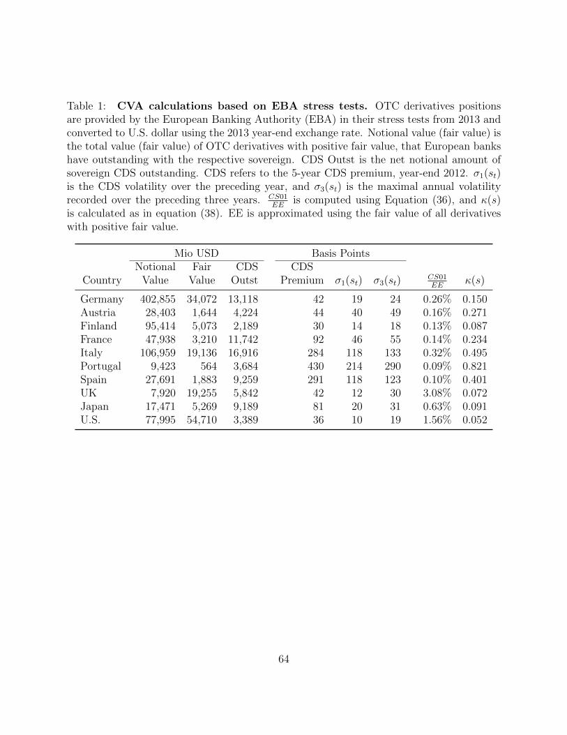
Table 1: CVA calculations based on EBA stress tests. OTC derivatives positionsare provided by the European Banking Authority (EBA) in their stress tests from 2013 andconverted to U.S. dollar using the 2013 year-end exchange rate. Notional value (fair value) isthe total value (fair value) of OTC derivatives with positive fair value, that European bankshave outstanding with the respective sovereign. CDS Outst is the net notional amount ofsovereign CDS outstanding. CDS refers to the 5-year CDS premium, year-end 2012. σ1(st)is the CDS volatility over the preceding year, and σ3(st) is the maximal annual volatilityrecorded over the preceding three years. CS01

EEis computed using Equation (36), and κ(s)

is calculated as in equation (38). EE is approximated using the fair value of all derivativeswith positive fair value.

Mio USD Basis PointsNotional Fair CDS CDS

Country Value Value Outst Premium σ1(st) σ3(st)CS01EE

κ(s)

Germany 402,855 34,072 13,118 42 19 24 0.26% 0.150Austria 28,403 1,644 4,224 44 40 49 0.16% 0.271Finland 95,414 5,073 2,189 30 14 18 0.13% 0.087France 47,938 3,210 11,742 92 46 55 0.14% 0.234Italy 106,959 19,136 16,916 284 118 133 0.32% 0.495Portugal 9,423 564 3,684 430 214 290 0.09% 0.821Spain 27,691 1,883 9,259 291 118 123 0.10% 0.401UK 7,920 19,255 5,842 42 12 30 3.08% 0.072Japan 17,471 5,269 9,189 81 20 31 0.63% 0.091U.S. 77,995 54,710 3,389 36 10 19 1.56% 0.052

64

Table 2: Banks’ derivatives exposures and CDS volumes outstanding. This tableshows the results of regressing the logarithm of the sovereign CDS net notional outstandingon the indicated variables. log(FV ) is the fair value of all derivatives positions with positivefair value, that European banks and banks in the UK have toward a sovereign. log(Debt) isthe total sovereign debt outstanding for the respective country. Data on the fair value of thederivatives positions are obtained from the EBA stress tests in December 2013 and December2015. The net notional CDS amounts outstanding are year-end obtained from the DTCCdatabase. Amounts of debt outstanding are obtained from countryeconomics.com. Het-eroskedasticity robust standard errors are reported in parenthesis. ∗∗∗ indicates significanceat a 1% level, and ∗∗ indicates significance at a 5% level.

(1) (2) (3) (4)

Intercept 13.70∗∗∗ 13.73∗∗∗ 6.96∗∗∗ 6.58∗∗∗

(0.89) (1.65) (1.41) (1.59)

Intercept ×1{2015} −0.05 0.81(1.95) (2.96)

log(FV ) 0.37∗∗∗ 0.37∗∗∗ 0.10∗∗∗ 0.11∗∗

(0.04) (0.08) (0.04) (0.05)

log(FV )× 1{2015} −0.01 0.00(0.09) (0.09)

log(Debt) 0.46∗∗∗ 0.48∗∗∗

(0.07) (0.07)

log(Debt)× 1{2015} −0.04(0.16)

Observations 55 55 55 55Adjusted R2 0.45 0.44 0.77 0.76

65

Table 3: Explaining bond yields with credit risk, risk-free rates, and convenienceyield. This table shows the results of a regression of the following form:

∆Y ieldt = α + βCDS∆CDSt + βrf∆rft + βCY ∆CYt + Controlst + εt.

Y ieldt is the 5-year bond yield of the most recently issued government bond, CDSt is the5-year CDS premium, rft denotes the risk-free rate proxy measured by 5-year overnightswap rates, CYt is a proxy for the convenience yield, measured as the difference betweenthe 3-month overnight swap rate and the 3-month bond yield for the respective sovereign.Controlst include changes in the turnover of Treasury bonds with 3 to 6 years to maturity orGilts with any maturity, changes in the 10-year on-the-run off-the-run spread, changes in thespread between KfW bond yields and German government bond yields, and changes in ourproxy for the cheapest-to-deliver option, embedded in sovereign CDS. Heteroscedasticity-robust standard errors are reported in parenthesis. * Significant at 10% level, ** Significantat 5% level, *** Significant at 1% level.

Japan U.S. Germany UK

Intercept −0.19∗ 0.04 −0.21 0.10(0.11) (0.13) (0.26) (0.35)

∆CDSt −0.01 −0.00 0.08 0.20∗

(0.02) (0.07) (0.09) (0.12)

∆Rft 0.82∗∗∗ 0.89∗∗∗ 0.87∗∗∗ 0.75∗∗∗

(0.06) (0.05) (0.06) (0.06)

∆CYt −0.07 0.03 −0.07 −0.15(0.11) (0.11) (0.06) (0.11)

∆OnOfft −0.33∗∗

(0.15)

∆Turnovert 0.99 0.62(0.67) (0.73)

∆KfWt −0.23∗∗∗

(0.06)

∆CtDt 0.17 1.99∗∗∗ 3.72∗∗∗ 4.25∗∗∗

(0.13) (0.60) (0.83) (0.74)

Observations 240 253 252 170Adjusted R2 0.73 0.96 0.84 0.86

66

Table 4: Cross-Sectional Tests. This table shows the results of a cross-sectionalregression of the following form:

∆Y ieldi,t = α+ βCDS∆CDSi,t + βrf∆rfi,t + εt.

Y ieldi,t is the 10-year bond yield of the most recently issued government bond forcountry i, CDSi,t is the 10-year CDS premium for country i, and rfi,t denotes therisk-free rate proxy measured by 10-year LIBOR swap rates. High EDF and highTED correspond to periods where the average G16 bank EDF and the treasury-eurodollar (TED) spread are above their 80% percentile, respectively. The percentileis computed over the entire sample period. The countries in the sample are classifiedas safe, low-risk, and risky, based on the average CDS premium in the entire sampleperiod. According to that measure, the sample of safe countries consists of Denmark,Finland, Germany, Netherlands, Norway, Sweden, UK, and the US. The sample oflow-risk countries consists of Austria, Belgium, China, Czech Republic, France, Japan,Slovakia. The sample of risky countries consists of Ireland, Italy, Poland, Portugal,Spain, Bulgaria, Slovenia, Romania. Heteroscedasticity-robust standard errors arereported in parenthesis. * Significant at 10% level, ** Significant at 5% level, ***Significant at 1% level.

(1) (2) (3) (4)

Intercept −0.23∗∗ −0.28∗∗∗ −0.28∗∗∗ −0.28∗∗∗

(0.09) (0.09) (0.09) (0.09)

∆CDSi,t 0.59∗∗∗ 0.62∗∗∗ 0.62∗∗∗ 0.62∗∗∗

(0.05) (0.04) (0.04) (0.04)

∆Rfi,t 0.82∗∗∗ 0.78∗∗∗ 0.78∗∗∗ 0.78∗∗∗

(0.07) (0.07) (0.07) (0.07)

∆CDSi,t × 1{i∈safe} −0.79∗∗∗ −0.79∗∗∗ −0.79∗∗∗

(0.07) (0.07) (0.07)

∆CDSi,t × 1{i∈low-risk} −0.24∗∗∗ −0.23∗∗∗ −0.23∗∗

(0.09) (0.08) (0.09)

∆CDSi,t × 1{i∈safe} × 1{EDFt≥q(80%)} 0.14∗

(0.08)

∆CDSi,t × 1{i∈low-risk} × 1{EDFt≥q(80%)} −0.45∗∗∗

(0.16)

∆CDSi,t × 1{i∈safe} × 1{TEDt≥q(80%)} 0.02(0.08)

∆CDSi,t × 1{i∈low-risk} × 1{TEDt≥q(80%)} −0.21∗∗∗

(0.05)

Observations 5,414 5,414 5,414 5,414Adjusted R2 0.48 0.50 0.50 0.50

67

Table 5: Sovereign CDS premiums, credit risk, and regulatory proxies. The table reportsparameter estimates and heteroskedasticity-robust t-statistics for regressions of the following form:

∆CDSt = α+βY S∆Y St + βCtD∆CtDt + βSwptn∆Swptnt + βEDF ∆EDFt + εt.

Y St is the difference between 5-year bond yield and 5-year overnight swap rate in the respectivecurrency. ∆CtDt is the change in our estimate of the cheapest-to-deliver option, embedded in thesovereign CDS. Swptnt is the (basis point) premium on an option to enter a 5-year swap position, asfixed payer or fixed receiver, in the respective currency, over the next 5 years. ∆EDFt is the residualof changes in the average of the Moody’s Expected Default Frequency (EDF) for the 16 largestderivatives dealing banks, regressed on changes in the yield spreads of the respective sovereign. Creditratio denotes the ratio of the adjusted R2 from a regression of ∆CDSt on ∆Y St and ∆CtDt to theadjusted R2 from the full regression specified above. The sample period is January 2010 to December2014, using weekly observations sampled each Wednesday. *Significant at 10% level. **Significant at5% level. ***Significant ant 1% level.

Adj. CreditIntercept βY S βCtD βSwptn βEDF R2 Ratio # Obs

Japan 0.01 0.14 -0.95 0.04* 0.13* 0.09 0.11 256[0.02] [0.4] [-0.73] [1.78] [1.68]

U.S. -0.08 0.04 -0.15 0 0.05*** 0.06 0.17 251[-0.49] [0.36] [-0.72] [0.18] [4.76]

Germany -0.04 0.06 -1.3** 0.04*** 0.16*** 0.35 0.17 256[-0.18] [0.91] [-2.43] [2.7] [4.93]

UK -0.24 0.18*** -0.54* 0.02 0.1*** 0.21 0.43 256[-1.11] [3.12] [-1.88] [1.06] [4.76]

Finland 0 0.11*** -0.2 0.01 0.14*** 0.43 0.16 242[-0.02] [3.32] [-1.32] [1.21] [6.12]

France 0.07 0.53*** 0.91 0.05** 0.4*** 0.57 0.51 256[0.16] [7.38] [1.41] [1.98] [6.65]

Austria -0.12 0.4*** 0.67 0.03 0.27*** 0.42 0.57 256[-0.29] [4.43] [1.06] [1.2] [4.17]

Italy 0.04 0.51*** 2.73 0.13** 0.74*** 0.64 0.75 256[0.04] [5.6] [1.33] [2.28] [6.43]

Spain -0.09 0.65*** 2.49* 0.08 0.4*** 0.66 0.94 256[-0.1] [8.11] [1.68] [1.23] [4.03]

Portugal 0.3 0.53*** 2.24 0.15 1.09*** 0.66 0.86 255[0.15] [6.64] [0.93] [0.9] [3.96]

68

Table 6: Link between corporate bond yields and CDS premiums. The table shows theresults of a regression of the following form:

∆Y ieldi,t = α+ βCDS∆CDSi,t + βrf∆rfi,t + εi,t.

Y ieldi,t is the bond yield of corporate bond i, CDSi,t is the maturity-matched CDS premium forbond i, rfi,t is the maturity-matched proxy for the risk-free rate (measured as LIBOR rate). Thesample period is July 2002 to December 2014. Heteroskedasticity robust standard errors, clusteredon bond level are reported in paranthesis. ∗∗∗, ∗∗, and ∗ indicate significance at a 1%, 5%, and 10%level respectively.

Aaa - Aa A Baa Ba-C

Intercept −0.00 −0.00 −0.00 −0.00(0.00) (0.00) (0.00) (0.00)

∆CDSt 0.42∗∗∗ 1.02∗∗∗ 0.93∗∗∗ 0.52∗∗∗

(0.04) (0.11) (0.05) (0.05)

∆rft 0.92∗∗∗ 0.89∗∗∗ 0.68∗∗∗ 0.02(0.02) (0.02) (0.04) (0.10)

Observations 19,629 20,249 20,414 29,562Adjusted R2 0.42 0.34 0.35 0.30

69

Table 7: Link between bond yields and CDS premiums in different episodes. The tableshows the results of a regression of the following form:

∆Y ieldi,t = α+ βCDS∆CDSi,t + βCDS∆CDSi,t × 1{Corporate} + βrf∆rfi,t + εi,t.

Y ieldi,t is the bond yield of bond i, CDSi,t is the maturity-matched CDS premium for bond i,1{Corporate} is a dummy variable that equals one if the underlying is a corporate bond issuer andzero if the underlying is a financial, rfi,t is the maturity-matched proxy for the risk-free rate(measured as LIBOR rate). Non-financials include bonds of non-financial corporations with Aaaor Aa rating. Financials include bonds of financial corporations with Aaa or Aa rating. Under Pre,the results for the July 2002 to June 2007 sub-period are reported. Under Crisis, the results for theJuly 2007 to December 2009 sub-period are reported. Under Post, the results for the January 2010– December 2014 sub-period are reported. Heteroskedasticity robust standard errors, clustered onbond level are reported in paranthesis. ∗∗∗, ∗∗, and ∗ indicate significance at a 1%, 5%, and 10%level respectively.

Pre Crisis Post

Intercept −0.00 0.00 0.00∗

(0.00) (0.00) (0.00)

∆CDSt 0.98∗∗∗ 0.48∗∗∗ 0.50∗∗∗

(0.09) (0.11) (0.07)

∆CDSt × 1{Corporate} −0.20 −0.10 −0.25∗∗

(0.27) (0.12) (0.11)

∆rft 0.90∗∗∗ 0.73∗∗∗ 0.96∗∗∗

(0.02) (0.05) (0.02)

Observations 36,153 12,842 19,823Adjusted R2 0.43 0.22 0.57

70

Additional Results (Online Appendix)

Table 8: Explaining bond yields with risk-free rates and credit riskThis table shows the results of a regression of the following form:

∆Y ieldt = α + βrf∆rft + βCDS∆CDSt + εt.

Y ieldt is the 5-year bond yield of the most recently issued government bond, rft denotes therisk-free rate proxy measured by 5-year overnight swap rates, and CDSt is the 5-year CDSpremium. Heteroscedasticity-robust standard errors are reported in parenthesis. Estimatesof the intercept are not reported for brevity. ** Significant at 5% level, *** Significant at 1%level.

βrf [std E] βCDS [std E] R2

Japan 0.79*** [0.07] -0.01 [0.02] 0.68U.S. 1.02*** [0.02] -0.01 [0.03] 0.95

Germany 1.13*** [0.05] 0.07 [0.09] 0.8UK 0.98*** [0.03] 0.23** [0.11] 0.79

Finland 1.13*** [0.05] 0.51*** [0.18] 0.69France 1.12*** [0.08] 0.54*** [0.11] 0.55

Austria 1.13*** [0.08] 0.6*** [0.16] 0.54Italy 0.98*** [0.32] 0.76*** [0.09] 0.42

Spain 0.88*** [0.24] 0.78*** [0.07] 0.58Portugal 1.61** [0.72] 0.98*** [0.08] 0.56

71

2011 2012 2013 2014

020

4060

8010

012

0

Bas

is p

oint

s

CDS premiumConvenience yield

Figure 7: CDS premium and bond convenience yield for Germany. The Figureshows the time series of the 5-year CDS premium and a proxy for the convenience yieldin the German government bonds. The convenience yield is approximated as the differencebetween the 3-month overnight swap rate (Eonia) and the 3-month German government bondyield, assuming that the 3-month government bond close to credit-risk free. All spreads arein basis points.

72

Table 9: Summary statistics for corporate bonds and CDS. This table providessummary statistics for a sample of corporate bonds obtained from TRACE. The sampleconsists of all corporate bonds with a credit rating, maturities between 3 years and 10years, and a matching credit default swap with no restructuring (docclause XR). For eachtrading day and each bond, the last traded yield is used. The matching CDS premium isobtained by interpolating the CDS premiums with the two nearest maturities. Swap ratesbased on the U.S. LIBOR curve are used as a proxy for the risk free rate. #obs per bondgives summary statistics for the time series of each bond (note that one corporation canissue several bonds). Avg Basis gives summary statistics for the average CDS bond basis,measured as the difference between CDS premium and bond yield minus risk-free rate. AvgTTM is the average time to maturity for each bond in the sample. The sample period isJuly 2002 to December 2014.

Mean SD Min Median Max N

Panel A: Aaa-Aa corporate bonds

#obs per bond 226 295 2 88 1382 87Avg Basis 0.10 0.18 −0.43 0.12 0.56 87Avg TTM 5.08 1.88 3.00 4.33 9.74 87

Panel B: A corporate bonds

#obs per bond 74 127 1.00 15 725 273Avg Basis −0.17 0.32 −1.90 −0.12 0.94 273Avg TTM 5.01 1.80 3.00 4.43 9.87 273

Panel C: Baa corporate bonds

#obs per bond 82 135.00 1 20 832 251Avg Basis −0.61 0.81 −8.09 −0.44 1.51 251Avg TTM 5.18 2.03 3.00 4.39 9.98 251

Panel D: Ba-C corporate bonds

#obs per bond 188 222 1 108 1000 158Avg Basis 0.14 1.58 −8.73 −0.01 5.15 158Avg TTM 5.52 1.93 3.02 5.07 9.98 158

Panel E: Aaa-Aa financials’ bonds

#obs per bond 162 218 1 56 1281 304Avg Basis −0.12 0.75 −3.11 −0.05 8.69 304Avg TTM 4.88 1.75 3.00 4.27 10.00 304

73

Table 10: Sovereign CDS premiums, credit risk, and regulatory proxies. Thetable reports parameter estimates and heteroskedasticity-robust t-statistics for regressions ofthe following form:

∆CDSt = α+βY S∆Y St + βSwptn∆Swptnt + βEDF ∆EDFt + εt.

Y St is the difference between 5-year bond yield and 5-year overnight swap rate in the respectivecurrency. Swptnt is the (basis point) premium on an option to enter a 5-year swap position, asfixed payer or fixed receiver, in the respective currency, over the next 5 years. ∆EDFt is theresidual of changes in the average of the Moody’s Expected Default Frequency (EDF) for the16 largest derivatives dealing banks, regressed on changes in the yield spreads of the respectivesovereign. Credit ratio denotes the ratio of the adjusted R2 from a regression of ∆CDSt on∆Y St to the adjusted R2 from the full regression specified above. The sample period is January2010 to December 2014, using weekly observations sampled each Wednesday. *Significant at10% level. **Significant at 5% level. ***Significant ant 1% level.

Adj. CreditIntercept βY S βSwptn βEDF R2 Ratio # Obs.

Japan 0.01 0.15 0.04* 0.13* 0.09 0.00 256[0.03] [0.45] [1.88] [1.72]

U.S. -0.08 -0.05 0.00 0.04** 0.01 0.00 256[-0.3] [-0.37] [-0.25] [2.18]

Germany -0.04 0.01 0.04*** 0.17*** 0.33 0.00 256[-0.17] [0.13] [2.98] [4.78]

UK -0.22 0.16*** 0.01 0.11*** 0.21 0.19 256[-1.04] [2.84] [0.97] [4.93]

Finland 0.04 0.13*** 0.02** 0.14*** 0.43 0.12 241[0.26] [3.66] [2.12] [6.14]

France 0.07 0.56*** 0.05* 0.39*** 0.56 0.52 256[0.17] [7.41] [1.95] [6.89]

Austria -0.10 0.43*** 0.03 0.26*** 0.41 0.59 256[-0.26] [4.49] [1.00] [4.10]

Italy -0.04 0.62*** 0.13** 0.73*** 0.63 0.76 256[-0.04] [10.76] [2.23] [6.14]

Spain -0.22 0.76*** 0.08 0.38*** 0.65 0.94 256[-0.23] [14.73] [1.21] [3.80]

Portugal 0.35 0.58*** 0.16 1.1*** 0.65 0.86 255[0.17] [12.05] [1.00] [4.06]

74