safe-dnn: a deep neural network with spike a f …

Under review as a conference paper at ICLR 2020

SAFE-DNN: A DEEP NEURAL NETWORK WITH SPIKEASSISTED FEATURE EXTRACTION FOR NOISE ROBUSTINFERENCE

Anonymous authorsPaper under double-blind review

ABSTRACT

We present a Deep Neural Network with Spike Assisted Feature Extraction (SAFE-DNN) to improve robustness of classification under stochastic perturbation ofinputs. The proposed network augments a DNN with unsupervised learning of low-level features using spiking neuron network (SNN) with Spike-Time-Dependent-Plasticity (STDP). The complete network learns to ignore local perturbation whileperforming global feature detection and classification. The experimental resultson CIFAR-10 and ImageNet subset demonstrate improved noise robustness formultiple DNN architectures without sacrificing accuracy on clean images.

1 INTRODUCTION

There is a growing interest in deploying DNNs in autonomous systems interacting with physicalworld such as autonomous vehicles and robotics. It is important that an autonomous systems makereliable classifications even with noisy data. However, in a deep convolutional neural networks (CNN)trained using stochastic gradient descent (SGD), pixel level perturbation can cause kernels to generateincorrect feature maps. Such errors can propagate through network and degrade the classificationaccuracy (Nazare et al. (2017); Luo & Yang (2014)).

Approaches for improving robustness of a DNN to pixel perturbation can be broadly divided intotwo complementary categories. First, many research efforts have developed image de-noising (orfiltering) networks that can pre-process an image before classification, but at the expense of additionallatency in the processing pipeline (Ronneberger et al. (2015); Na et al. (2019); Xie et al. (2012);Zhussip & Chun (2018); Soltanayev & Chun (2018); Zhang et al. (2017)). De-noising is an effectiveapproach to improve accuracy under noise but can degrade accuracy for clean images (Na et al.(2019)). Moreover, de-noising networks trained on a certain noise type do not perform well if thea different noise structure is experienced during inference (Zhussip & Chun (2018)). Advancedde-noising networks are capable of generalizing to multiple levels of a type of noise and effective fordifferent noise types (Zhussip & Chun (2018); Soltanayev & Chun (2018); Zhang et al. (2017)). Buthigh complexity of these network makes them less suitable for real-time applications and lightweightplatforms with limited computational and memory resources.

An orthogonal approach is to develop a classification network that is inherently robust to inputperturbations. Example approaches include training with noisy data, introducing noise to networkparameters during training, and using pixel level regularization (Milyaev & Laptev (2017); Nazareet al. (2017); Luo & Yang (2014); Na et al. (2018); Long et al. (2019)). These approaches do notchange the processing pipeline or increase computational and memory demand during inference.However, training-based approaches to design robust DNNs also degrade classification accuracy forclean images, and more importantly, are effective only when noise structure (and magnitude) duringtraining and inference closely match. Therefore, a new class of DNN architecture is necessary forautonomous system that is inherently resilient to input perturbations of different type and magnitudewithout requiring training on noisy data, as well as computationally efficient.

Towards this end, this paper proposes a new class of DNN architecture that integrates featuresextracted via unsupervised neuro-inspired learning and supervised training. The neuro-inspiredlearning, in particular, spiking neural network (SNN) with spike-timing-dependent plasticity (STDP)is an alternative and unsupervised approach to learning features in input data (Hebb et al. (1950);

1


3x32 32x40 40x44 64x128

128x10 f.c.Input

3x16 16x30 30x20

Spiking convolution module

Main CNN moduleAuxiliary CNN module

⋯

Weight

X

Batch normalization

SAU

Conductance Matrix

X

Spiking Neuron

Spike Conversion

Re-scale

Insert

Convert

(a) (b)

SNN learning DNN training and inference

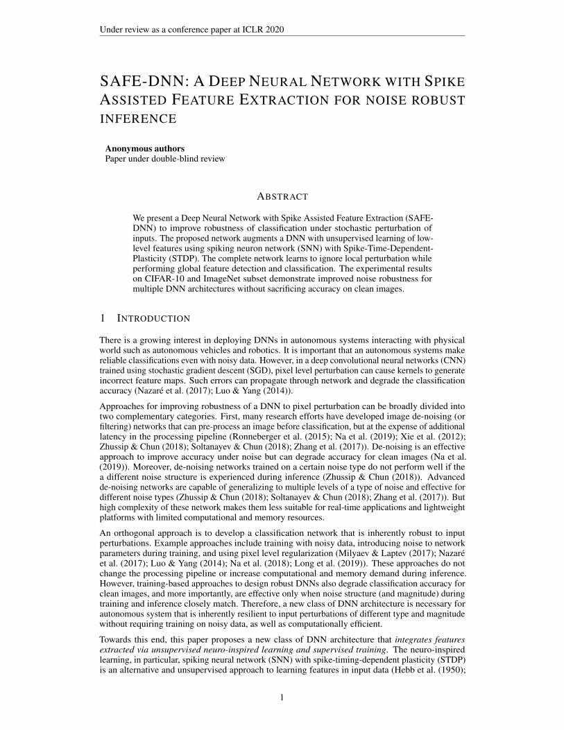
Figure 1: (a) An example architecture of SAFE-DNN. (b) Transition of building blocks from SNN to spikingconvolution module of SAFE-DNN, with a special activation unit (SAU)

Bi & Poo (2001); Diehl & Cook (2015); She et al. (2019a); Querlioz et al. (2013); Srinivasan et al.(2016)). STDP based SNN optimizes network parameters according to causality information with nolabels (Moreno-Bote & Drugowitsch (2015); Lansdell & Kording (2019)). However, the classificationaccuracy of a STDP-learned SNN for complex datasets is much lower than a that of a DNN.

The fundamental premise of this paper is that, augmenting the feature space of a supervised (trained)DNN with features extracted by an SNN via STDP-based learning increases robustness of the DNNto input perturbations. We argue that stochastic gradient descent (SGD) based back-propagationin a DNN enables global learning between low-level pixel-to-pixel interactions and high-leveldetection and classification. On the other hand, STDP performs unsupervised local learning andextracts low-level features under spatial correlation. By integrating features from global (supervisedtraining) and local (STDP) learning, the hybrid network “learns to ignore” locally uncorrelatedperturbations (noise) in pixels while extracting the correct feature representation from the overallimage. Consequently, hybridization of SGD and STDP enables robust image classification undernoisy input while preserving the accuracy of the baseline DNN for clean images.

We present a hybrid network architecture, referred to as Spike Assisted Feature Extraction basedDeep Neural Network (SAFE-DNN), to establish the preceding premise. We develop an integratedlearning/training methodology to couple the features extracted via neuro-inspired learning andsupervised training. In particular, this paper makes the following contributions:

• We present a SAFE-DNN architecture (Figure 1) that couples STDP-based robust learningof local features with SGD based supervised training. This is achieved by integrating aspiking convolutional module within a DNN pipeline.• We present a novel frequency-dependent stochastic STDP learning rule for the spiking

convolutional demonstrating local competitive learning of low level features. The proposedlearning method makes the feature extracted by the spiking convolutional module robust tolocal perturbations in the input image.• We develop a methodology to transform the STDP-based spiking convolution to an equiv-

alent CNN. This is achieved by using a novel special neuron activation unit (SAU), anon-spiking activation function, that facilitates integration of the SNN extracted featureswithin the DNN thereby creating a single fully-trainable deep network. The supervised(SGD-based) training is performed in that deep network after freezing the STDP-learntweights in the spiking CNN module.

We present implementations of SAFE-DNN based on different deep networks including MobileNet,ResNet and DenseNet (Sandler et al. (2018), He et al. (2015), Huang et al. (2016)) to show theversatility of our network architecture. Experiment is conducted for CIFRA10 and ImageNet subsetconsidering different types of noise, including Gaussian, Wald, Poisson, Salt&Paper, and adversarialnoise demonstrating robust classification under input noise. Unlike training-based approaches,SAFE-DNN shows improved accuracy for a wide range of noise structure and magnitude withoutrequiring any prior knowledge of the perturbation during training and inference and does not degradethe accuracy for clean images (even shows marginal improvement in many cases). SAFE-DNN

2


complements, and can be integrated with, de-noising networks for input pre-processing. However,unlike de-noising networks, the SAFE-DNN has negligible computation and memory overhead,and does not introduce new stages in the processing pipeline. Hence, SAFE-DNN is an attractivearchitecture for resource-constrained autonomous platforms with real-time processing.

We note that, SAFE-DNN differs from deep SNNs that convert a pre-trained DNN to SNN (Senguptaet al. (2019), Hu et al. (2018)). Such networks function as a spiking network during inference toreduce energy; however, the learning is still based on supervision and back-propagation. In contrast,SAFE-DNN hybridizes STDP and SGD during learning but creates a single hybrid network operatingas a DNN during inference.

2 BACKGROUND ON SNN

Spiking neural network uses biologically plausible neuron and synapse models that can exploittemporal relationship between spiking events (Moreno-Bote & Drugowitsch (2015); Lansdell &Kording (2019)). There are different models that are developed to capture the firing pattern of realbiological neurons. We choose to use Leaky Integrate Fire (LIF) model in this work described by:

dv/dt = a+ bv + cI; and v = vreset, if v > vthreshold (1)

where, a, b and c are parameters that control neuron dynamics, and I is the sum of current signalfrom all synapses that connects to the neuron.

In SNN, two neurons connected by one synapse are referred to as pre-synaptic neuron and post-synaptic neuron. Conductance of the synapse determines how strongly two neurons are connected andlearning is achieved through modulating the conductance following an algorithm named spike-timing-dependent-plasticity (STDP) (Hebb et al. (1950); Bliss & Gardner-Medwin (1973); Gerstner et al.(1993)). With two operations of STDP: long-term potentiation (LTP) and long-term depression (LTD),SNN is able to extract the causality between spikes of two connected neurons from their temporalrelationship. More specifically, LTP is triggered when post-synaptic neuron spikes closely after apre-synaptic neuron spike, indicating a causal relationship between the two events. On the otherhand, when a post-synaptic neuron spikes before pre-synaptic spike arrives or without receiving apre-synaptic spike at all, the synapse goes through LTD. For this model the magnitude of modulationis determined by (Querlioz et al. (2013)):

∆Gp = αpe−βp(G−Gmin)/(Gmax−Gmin) and ∆Gd = αde

−βd(Gmax−G)/(Gmax−Gmin) (2)

In the functions above, ∆Gp is the magnitude of LTP actions, and ∆Gd is the magnitude of LTDactions. αp, αd, βp, βd, Gmax and Gmin are parameters that are tuned based on specific networkconfigurations.

3 MOTIVATION BEHIND SAFE-DNN

The gradient descent based weight update process in a DNN computes the new weight as W ′ = W −η∇L, where the gradient of loss function L is taken with respect to weight: ∇wL = 〈 ∂L∂Wi

, ..., ∂L∂Wk〉.

Consider cross entropy loss as an example for L, weight optimization of element i is described by:

W ′i = Wi − η− 1N ∂{

N∑n=1

[ynlog(yn)]}

∂Wi(3)

Here η is the rate for gradient descent; N is the number of classes; yn is a binary indicator for thecorrect label of current observation and yn is the predicated probability of class n by the network.For equation (3), gradient is derived based on the output prediction probabilities y and ground truth.Such information is available only at the output layer. To generate the gradient, the output prediction(or error) has to be back-propagated from the output layer to the target layer using chain rule. Asy = g(W,X) with g being the logistic function and X the input image, the prediction probabilitiesare the outcome of the entire network structure. Consider the low level feature extraction layers in adeep network. Equation (3) suggests that gradient of the loss with respect to a parameter is affected

3


by all pixels in the entire input image. In other words, the back-propagation makes weight updatesensitive to non-neighboring pixels. This facilitates global learning and improve accuracy of higherlevel feature detection and classification.

However, the global learning also makes it difficult to strongly impose local constraints during training.Hence, the network does not learn to ignore local perturbations during low-level feature extraction asit is trained to consider global impact of each pixel for accurate classifications. This means that duringinference, although a noisy pixel is an outlier from the other pixels in the neighbourhood, a DNNmust consider that noise as signal while extracting low-level features. The resulting perturbationfrom pixel level noise propagates through the network, and degrades the classification accuracy.

The preceding discussion suggests that, to improve robustness to stochastic input perturbation (noise),the low level feature extractors must learn to consider local spatial correlation. The local learningwill allow network to more effectively “ignore” noisy pixels while computing the low-level featuremaps and inhibit propagation of input noise into the DNN pipeline.

The motivation behind SAFE-DNN comes from the observation that STDP in SNN enables locallearning of features. Compared to conventional DNN, SNN conductance is not updated throughgradient descent that depends on back propagation of global loss. Consider a network with onespiking neuron and n connected input synapses, a spiking event of the neuron at time tspike andtiming of closest spikes from all input spike trains Tinput, the modulated conductance is given by:

G′i = Gi + sign(∆ti) · r(Gi) · p(∆ti, fi) (4)

Here ∆ti = tspike − T iinput is spike timing difference, r is the magnitude function (Equation 2) andp is the modulation probability function (Equation 5). The value of tspike is a result of the neuron’sresponse to the collective sum of input spike trains in one kernel. Hence, the modulation of weight ofeach synapse in a SNN depends only on other input signals within the same (local) receptive field.Moreover, as the correlation between the spike patterns of neighboring pre-synaptic neurons controlsand causes the post-synaptic spike, STDP helps the network learn the expected spatial correlationbetween pixels in a local region. During inference, if the input image contains noise, intensity ofindividual pixel can be contaminated but within a close spatial proximity the correlation is betterpreserved. As the SNN has learned to respond to local correlation, rather than individual pixels, theneuron’s activity experiences less interference from local input perturbation. In other words, the SNN“learns to ignore” local perturbations and hence, the extracted features are robust to noise.

4 SAFE-DNN ARCHITECTURE AND LEARNING PROCESS

4.1 NETWORK ARCHITECTURE

Table 1: Network Complexity

Model Params (M) MACs (G)

Baseline MobileNetV2 3.50 0.33Baseline ResNet101 44.55 7.87Baseline DenseNet121 7.98 2.90

SAFE-MobileNetV2 3.57 0.36SAFE-ResNet101 44.62 7.90SAFE-DenseNet121 8.04 2.94

Fig. 1 (a) shows an illustrative implementa-tion of SAFE-DNN. The network containsspiking layers placed contiguously to formthe spiking convolution module, along withconventional CNN layers. The spiking convo-lution module is placed at the front to enablerobust extraction of local and low-level fea-tures. Further, to ensure that the low-levelfeature extraction also considers global learn-ing, which is the hallmark of gradient back-propagation as discussed in section 3, we place several conventional CNN layers of smaller sizein parallel with the spiking convolution module. This is called the auxiliary CNN module. Theoutput feature map of the two parallel modules is maintained to have the same height and width, andconcatenated along the depth to be used as input tensor to the remaining CNN layers, referred to asthe main CNN module. Main CNN module is responsible for higher level feature detection as wellas the final classification. The main CNN module can be designed based on existing deep learningmodels. The concatenation of features from auxilary CNN and spikining convolutional module helpsintegrate global and local learning.

4


Conv2d

2242x3

Channel32

Bottleneck

1122x32

Channel16

Bottleneck

1122x16

Channel24

Fully Connect

1x1x1280

Channel𝒩

⋯

MobilenetV2 original

Main CNN module

Spiking convolution

module

Auxiliary CNN module

SAFE-MobilenetV2

Drop

Clone

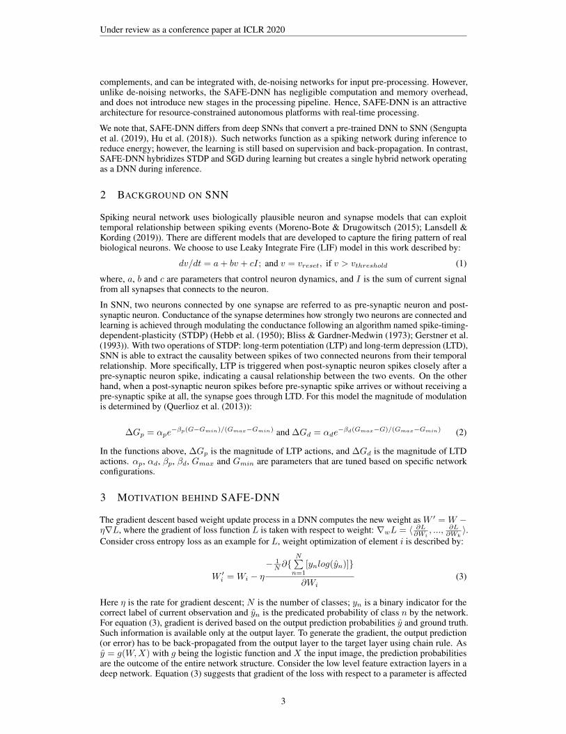
Figure 2: Creating SAFE-MobileNetV2 from the original MobileNetV2

Fig. 2 shows the process of implementing SAFE-MobileNetV2 based on the original MobileNetV2.The first convolution layer and the following one block from the original network architecture aredropped and the remaining layers are used as the mian CNN module of SAFE-MobileNetV2. Weshow that SAFE-DNN is a versatile network by testing three configurations in this work, which havethe main CNN module based on MobileNetV2, ResNet101 and DenseNet121, respectively. Thestorage and computational complexity of the networks are shown in Table 1. It can be observed thatSAFE-DNN implementations do not introduce a significant overhead to the baseline networks.

In the dynamical system of SNN, neurons transmit information in the form of spikes, which aretemporally discrete events that spread across multiple simulation time steps. This requires inputsignal intensity to be converted to spike trains, and a number of time steps for neurons to respondto input stimulus. Such mechanism is different from that of the conventional DNN, which takesonly one time step for data to propagate through the network. Due to this reason the native SNNmodel can not be used in spiking convolution module of SAFE-DNN. Two potential solutions to thisproblem are, running multiple time steps for every input, or, adapting the spiking convolution moduleto single-time-step response system. Since the first slows down both training and inference by at leastone order of magnitude, we choose the latter.

Training Process. We separate STDP-based learning and DNN training into two stages. In the firststage, the spiking convolution module operates in isolation and learns all images in the training setwithout supervision. The learning algorithm follows our novel frequency dependent STDP methoddescribed next in section 4.2. In the second stage, network parameters are first migrated to the spikingconvolution module of SAFE-DNN. The network building blocks of the spiking convolutional modulego through a conversion process shown in Fig. 1 (b). The input signal to spike train conversionprocess is dropped, and conductance matrix is re-scaled to be used in the new building block. Batchnormalization is inserted after the convolution layer. In order to preserve the non-linear property ofspiking neurons, a special activation unit (SAU) is designed to replace the basic spiking neuron model.Details about SAU is discussed later in section 4.3. Once the migration is completed, the entireSAFE-DNN is then trained fully using statistical method, while weights in the spiking convolutionmodule are kept fixed to preserve features learned by SNN. Network inference is performed using thenetwork architecture created during the second stage of training i.e. instead of the baseline LIF, theSAU is used for modeling neurons.

4.2 SPIKING CONVOLUTIONAL MODULE

Frequency-dependent stochastic STDP The STDP algorithm discussed in 2 captures the basic ex-ponential dependence on timing of synaptic behavior, but does not address the associative potentiationissue in STDP ( Levy & Steward (1979); Carew et al. (1981); Hawkins et al. (1983)). Associativity isa temporal specificity such that when a strong (in case of our SNN model, more frequent) input and aweak (less frequent) input into one neuron induce a post-synaptic spike, a following conductancemodulation process is triggered equivalently for the both.

In the context of STDP based SNN, associativity can cause erroneous conductance modulation ifunaccounted for (She et al. (2019b)). Therefore, we propose a frequency-dependent (FD) stochasticSTDP that dynamically adjust the probability of LTP/LTD based on input signal frequency. Thealgorithm is described by:

5


⋯ ⋯ ⋯

Inhibition

Layer 1 learning phase

Layer 2 learning phaseFrequency boost

⋯Spike

Conversion

Input image

Figure 3: The architecture of the spiking convolutional module for feature extraction and layer-by-layer learning process.

Pp = γpe(−∆t/(τp(1+φp

f−fminfmax−fmin

))) and Pd = γde(∆t/(τd(1+φd

f−fminfmax−fmin

))) (5)

In this algorithm, τd and τp are time constant parameters. ∆t is determined by subtracting the arrivaltime of the pre-synaptic spike from that of the post-synaptic spike (tpost − tpre). Probability of LTPPp is higher with smaller ∆t, which indicates a stronger causal relationship. The probability of LTDPd is higher when ∆t is larger. γp and γd controls the peak value of probabilities. fmax and fmindefine the upper and lower limit of input spike frequency and f is the value of input spike frequency.When input spike originates from a weak input, the probability declines faster than that from a stronginput. As a result, pre-synaptic spike time of weak input needs to be much closer to the post-synapticspike than that of strong input to have the same probability of inducing LTP, i.e. the window forLTP is narrower for weak input. The same rule applies to LTD behavior. As will be shown in thefollowing section, FD stochastic STDP exhibits better learning capability than conventional STDP.

SNN architecture The architecture of the spiking convolutional module is shown in Fig. 3. Thisarchitecture resembles conventional DNN but have some differences. First, the 8-bit pixel intensityfrom input images is converted to spike train with frequency over a range from fmin to fmax. Theinput spike train matrix connects to spiking neurons in the spiking convolution layer in the same wayas conventional 2D convolution, which also applies for connections from one spiking convolutionlayer to the next. All connections as mentioned are made with plastic synapses following STDPlearning rule. When a neuron in the convolution layer spikes, inhibitory signal is sent to neurons atthe same (x,y) coordinate across all depth in the same layer. This cross-depth inhibition prevents allneurons at the same location from learning the same feature. Overall, such mechanism achieves acompetitive local learning behavior of robust low level features that are crucial to the implementationof SAFE-DNN.

18 20 22 24 26Pre-synaptic spike frequency

0

10

20

30

Post

-syn

aptic

spi

ke fr

eque

ncy

Vth = -69.2Vth = -71.2Vth = -73.2

Pre-synaptic spiking frequency

Post

-syn

aptic

spi

king

frequ

ency

Figure 4: Post-synaptic spiking frequency (Hz)vs. pre-synaptic spike frequency (Hz)

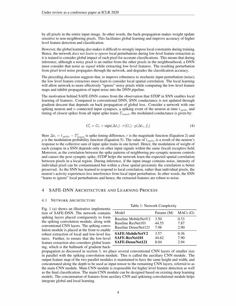
A basic property of spiking neuron is that a num-ber of spikes need to be received before a neuronreaches spiking state and emits one spike. In a twolayer network this does not cause a problem but formultiple-layer network it prohibits spiking signal totravel deep down. Due to the diminishing spikingfrequency of multiple-layer SNN, a layer-by-layerlearning procedure is used. When the first layer com-pletes learning, its conductance matrix is kept fixedand cross-depth inhibition disabled. Next, all neu-rons in the first layer are adjusted to provide higherspiking frequency by lowering the spiking thresholdVth. The effect of changing Vth is illustrated in Fig.4.In such way, neurons in the first layer receive input

from input images and produce enough spikes that can facilitate learning behavior of the second layer.The same process is repeated until all layers complete learning.

4.3 SPECIAL ACTIVATION UNIT

Consider the spike conversion process of SNN, given an input value of X ∈[0, 1]

and inputperturbation ξ, conversion to spike frequency with range ε ∈

[fmin, fmax

]is applied such that

6


F = Clipε{(X + ξ)(fmax − fmin)}. For the duration of input signal Tinput, the total receivedspikes for the recipient is Nspike = bF ∗Tinputc. Also consider how one spiking neuron responses toinput frequency variation, which is shown in Fig.4: it can be observed that flat regions exist throughoutspiking activity as its unique non-linearity. Therefore, for |ξ| ≤ δ

Tinput(fmax−fmin) perturbation doesnot cause receiving neuron to produce extra spikes. While the exact value of δ changes with differentinput frequency, it is small only when original input frequency is near the edges of non-linearity. Thisprovides the network with extra robustness to small input perturbations. Based on this, we design the

Special Activation Unit (SAU) to be a step function in the form of f(x) =n∑i=1

αiχi(x) where αi and

χi are pre-defined multiplication parameter and interval indicator function.

5 EXPERIMENTAL RESULTS

5.1 CIFAR10 DATASET

0 50 100 150Epoch

0

0.5

1

1.5

2

Loss

train loss test loss

0 50 100 150Epoch

20

40

60

80

100

Accu

racy

train accuracy test accuracy

0 50 100 150Epoch

0

0.5

1

1.5

2

Loss

train loss test loss

0 50 100 150Epoch

20

40

60

80

100

Accu

racy

train accuracy test accuracy

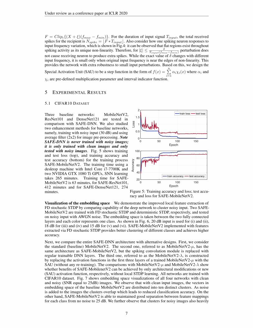
Figure 5: Training accuracy and loss; test accu-racy and loss for SAFE-MobileNetV2.

Three baseline networks: MobileNetV2,ResNet101 and DenseNet121 are tested incomparison with SAFE-DNN. We also studiedtwo enhancement methods for baseline networks,namely, training with noisy input (30 dB) and usingaverage filter (2x2) for image pre-processing. NoteSAFE-DNN is never trained with noisy images;it is only trained with clean images and onlytested with noisy images. Fig. 5 shows trainingand test loss (top), and training accuracy andtest accuracy (bottom) for the training processSAFE-MobileNetV2. The training time using adesktop machine with Intel Core i7-7700K andtwo NVIDIA GTX 1080 Ti GPUs, SNN learningtakes 265 minutes. Training time for SAFE-MobileNetV2 is 63 minutes, for SAFE-ResNet101,412 minutes and for SAFE-DenseNet121, 274minutes.

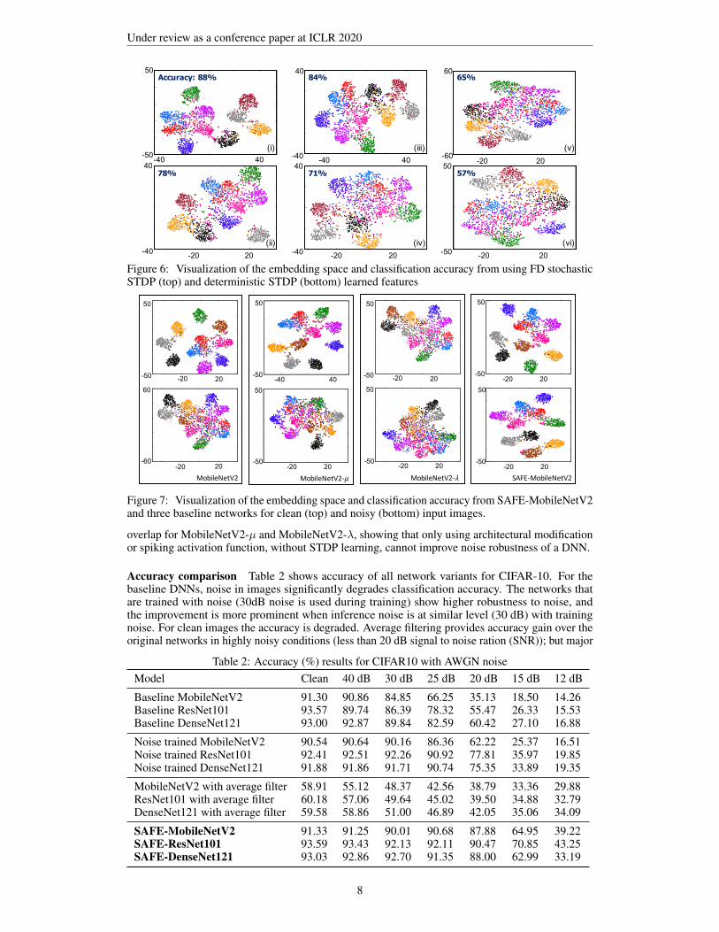
Visualization of the embedding space We demonstrate the improved local feature extraction ofFD stochastic STDP by comparing capability of the deep network to cluster noisy input. Two SAFE-MobileNetV2 are trained with FD stochastic STDP and deterministic STDP, respectively, and testedon noisy input with AWGN noise. The embedding space is taken between the two fully connectedlayers and each color represents one class. As shown in Fig. 6, 20 dB input is used for (i) and (ii),18 dB for (iii) and (iv) and 15 dB for (v) and (vi). SAFE-MobileNetV2 implemented with featuresextracted via FD stochastic STDP provides better clustering of different classes and achieves higheraccuracy.

Next, we compare the entire SAFE-DNN architecture with alternative designs. First, we considerthe standard (baseline) MobileNetV2. The second one, referred to as MobileNetV2-µ, has thesame architecture as SAFE-MobileNetV2, but the spiking convolution module is replaced withregular trainable DNN layers. The third one, referred to as the MobileNetV2-λ, is constructedby replacing the activation functions in the first three layers of a trained MobileNetV2-µ with theSAU (without any re-training). The comparisons with MobileNetV2-µ and MobileNetV2-λ showwhether benefits of SAFE-MobilenetV2 can be achieved by only architectural modifications or new(SAU) activation function, respectively, without local STDP learning. All networks are trained withCIFAR10 dataset. Fig. 7 shows embedding space visualizations of all four networks with cleanand noisy (SNR equal to 25dB) images. We observe that with clean input images, the vectors inembedding space of the baseline MobileNetV2 are distributed into ten distinct clusters. As noiseis added to the images the clusters overlap which leads to reduced classification accuracy. On theother hand, SAFE-MobileNetV2 is able to maintained good separation between feature mappingsfor each class from no noise to 25 dB. We further observe that clusters for noisy images also heavily

7


Accuracy: 23%

-50

50

40-40

-40

40-40 -20 0 20 40

-40

-20

0

20

40

60

-40 -20 0 20 40-40

-20

0

20

40-60 -40 -20 0 20 40 60

-40

-20

0

20

4084%

-40 -20 0 20 40-40

-20

0

20

40-40 -20 0 20 40

-60

-40

-20

0

20

40

60

-40 -20 0 20 40-50

0

50

20-20 -40

40

20-20 -50

50

20-20

-40

40

40-40 -60

60

20-20(i)

Accuracy: 88%

78%

(iii) (v)

(ii) (iv) (vi)

71% 57%

65%

Figure 6: Visualization of the embedding space and classification accuracy from using FD stochasticSTDP (top) and deterministic STDP (bottom) learned features

-40 -20 0 20 40-60

-40

-20

0

20

40-40 -20 0 20 40

-40

-20

0

20

40

60

3806195742-50 -20 20

50

-60-20 20

60

MobileNetV2-40 -20 0 20 40

-60

-40

-20

0

20

40-50 0 50

-100

-50

0

50

100806195742

40-40-50

50

-50-20 20

50

MobileNetV2-𝜇-40 -20 0 20 40

-60

-40

-20

0

20

40

60

380619574

-40 -20 0 20 40-50

0

50806195742

-50

50

-20 20

-50

50

-20 20SAFE-MobileNetV2

-40 -20 0 20 40-40

-20

0

20

40

60

-50

50

-50-20 20

50

MobileNetV2-𝜆

-20 20-40 -20 0 20 40-60

-40

-20

0

20

40

38061957

Figure 7: Visualization of the embedding space and classification accuracy from SAFE-MobileNetV2and three baseline networks for clean (top) and noisy (bottom) input images.

overlap for MobileNetV2-µ and MobileNetV2-λ, showing that only using architectural modificationor spiking activation function, without STDP learning, cannot improve noise robustness of a DNN.

Accuracy comparison Table 2 shows accuracy of all network variants for CIFAR-10. For thebaseline DNNs, noise in images significantly degrades classification accuracy. The networks thatare trained with noise (30dB noise is used during training) show higher robustness to noise, andthe improvement is more prominent when inference noise is at similar level (30 dB) with trainingnoise. For clean images the accuracy is degraded. Average filtering provides accuracy gain over theoriginal networks in highly noisy conditions (less than 20 dB signal to noise ration (SNR)); but major

Table 2: Accuracy (%) results for CIFAR10 with AWGN noiseModel Clean 40 dB 30 dB 25 dB 20 dB 15 dB 12 dB

Baseline MobileNetV2 91.30 90.86 84.85 66.25 35.13 18.50 14.26Baseline ResNet101 93.57 89.74 86.39 78.32 55.47 26.33 15.53Baseline DenseNet121 93.00 92.87 89.84 82.59 60.42 27.10 16.88

Noise trained MobileNetV2 90.54 90.64 90.16 86.36 62.22 25.37 16.51Noise trained ResNet101 92.41 92.51 92.26 90.92 77.81 35.97 19.85Noise trained DenseNet121 91.88 91.86 91.71 90.74 75.35 33.89 19.35

MobileNetV2 with average filter 58.91 55.12 48.37 42.56 38.79 33.36 29.88ResNet101 with average filter 60.18 57.06 49.64 45.02 39.50 34.88 32.79DenseNet121 with average filter 59.58 58.86 51.00 46.89 42.05 35.06 34.09

SAFE-MobileNetV2 91.33 91.25 90.01 90.68 87.88 64.95 39.22SAFE-ResNet101 93.59 93.43 92.13 92.11 90.47 70.85 43.25SAFE-DenseNet121 93.03 92.86 92.70 91.35 88.00 62.99 33.19

8


Table 3: Top 1 Accuracy (%) results for ImageNet subset with noiseModel Clean 25 dB 15 dB 10 dB 5 dB

Baseline MobileNetV2 70.80 67.41 57.92 45.35 34.48Baseline ResNet101 71.02 67.81 64.04 46.27 35.47Baseline DenseNet121 70.92 67.60 63.28 44.34 27.50

Noise trained MobileNetV2 66.30 68.12 59.71 46.70 34.66Noise trained ResNet101 68.91 69.20 65.71 52.60 41.32Noise trained DenseNet121 69.13 70.51 66.47 52.76 36.32

MobileNetV2 with average filter 67.44 66.91 61.69 51.69 40.43ResNet101 with average filter 68.18 68.25 65.14 53.09 41.50DenseNet121 with average filter 65.38 64.56 62.40 50.65 39.40

SAFE-MobileNetV2 71.05 67.86 65.91 53.82 42.33SAFE-ResNet101 71.14 70.67 67.24 55.04 42.87SAFE-DenseNet121 70.81 69.44 65.47 54.30 40.84

performance drop is observed under mild to no noise. This is expected as average filtering results insignificant loss of feature details for input images in the CIFAR-10 dataset.

For SAFE-DNN implemented with all three DNN architectures, performance in noisy condition isimproved over the original network by an appreciable margin. For example, at 20 dB SNR SAFE-MobileNetV2 remains at good performance while the original network drops below 40% accuracy,making a significant (50%) gain. Similar trend can be observed for other noise levels. Compared tonetworks trained with noise, SAFE-DNN shows similar performance at around 30 dB SNR while itsadvantage increases at higher noise levels. Moreover, for clean images accuracy of SAFE-DNN is onpar with the baseline networks.

5.2 TEST ON IMAGENET SUBSET Table 4: Top 5 Accuracy (%) results for MobileNetV2on ImageNet subset with Noise

Model Clean 10 dB 5 dB

Baseline 94.72 79.20 67.15Noise trained 92.43 81.63 68.36Average filtering 92.81 85.37 78.95SAFE-MobileNetV2 95.91 89.57 83.92

Considering the use case scenario of au-tonomous vehicles, we conduct test on a sub-set of ImageNet that contains classes relatedto traffic (cars, bikes, traffic signs, etc).Thesubset contains 20 classes with a total of26,000 training images. The same baselinenetworks as in the CIFAR10 test are used.Here 25 dB SNR images are used for noisetraining. The accuracy result is shown in Table 3. All networks achieve around 70% top 1 accuracyon clean images. Noise training shows robustness improvement over the baseline network but stillnegatively affects clean image accuracy. In this test the average filter shows less degradation underno noise condition than for the CIFAR10 test, due to higher resolution of input images. DensNet121shows more noise robustness than MobileNetV2 and ResNet101 when noise training is used, whilefor average filtering ResNet101 benefits the most. SAFE-DNN implementations of all three net-works exhibit same or better robustness over all noise levels. Clean image classification accuracyis also unaffected. Comparing top 5 accuracy result for SAFE-MobileNetV2 and its baselines, asshown in Table 4, SAFE-MobileNetV2 is able to maintain above 80% accuracy even at 5 dB SNR,outperforming all three baselines.

5.3 MORE PERTURBATION STRUCTURES

Random perturbation We test SAFE-DNN in three more noise structures: Wald, Poisson andsalt-and-pepper (SP). For CIFAR10, the result is shown in 5. Wald I has a distribution of µ =3, scale = 0.3 and for Wald II, µ = 13, scale = 1; Poisson I has a distribution with peak of 255and for Poisson II, 75; S&P I has 5% noisy pixels and S&P II has 20%. Noise-trained DNNs forWald, Poisson, and SP, are trained with noisy images generated using distributions Wald I, Poisson I,and SP I, resepectively. It can be observed that SAFE-DNN implementation with all three networksare more noise robust than baseline and average filtering. The noise-trained networks performs wellwhen inference noise is aligned with training noise, but performance drops when noise levels arenot aligned. Moreover, noise-trained networks trained with mis-aligned noise types performs poorly

9


Table 5: Accuracy (%) results for CIFAR10 with different noise typesModel Wald I Wald II Poisson I Poisson II S&P I S&P II

Baseline MobileNetV2 83.81 48.41 63.88 37.70 68.86 32.37Baseline ResNet101 85.12 60.75 76.49 56.47 79.25 47.69Baseline DenseNet121 87.34 63.24 78.15 60.60 83.50 49.54

Noise trained MobileNetV2 90.06 71.80 87.18 74.51 88.86 63.84Noise trained ResNet101 91.95 88.15 89.63 81.16 90.78 74.43Noise trained DenseNet121 91.48 84.42 89.44 78.90 89.93 72.24

MobileNetV2 w/ average filter 53.12 36.70 54.40 35.84 51.35 31.29ResNet101 w/ average filter 54.06 38.03 56.75 38.59 52.19 34.25DenseNet121 w/ average filter 55.86 39.69 56.31 37.34 51.61 32.47

SAFE-MobileNetV2 90.46 88.50 84.35 82.58 89.17 80.83SAFE-ResNet101 92.97 90.75 88.91 87.22 90.53 86.75SAFE-DenseNet121 92.83 89.52 87.67 85.75 90.28 85.38

Table 6: Accuracy (%) results for ImageNet subset with different noise typesModel Wald I Wald II Poisson I Poisson II S&P I S&P II

Baseline MobileNetV2 68.56 58.99 65.16 51.08 66.53 46.81Noise trained MobileNetV2 69.07 62.12 67.31 60.22 67.99 53.86MobileNetV2 w/ average filter 66.05 61.46 64.52 59.91 62.07 45.50SAFE-MobileNetV2 70.19 64.37 66.74 63.15 67.10 58.91

(results not shown). As for ImageNet subset, networks based on MobileNetV2 are tested. Wald I is adistribution with µ = 5, scale = 0.3 and Wald II is a distribution with µ = 25, scale = 1; Poisson Ihas a distribution with peak of 255 and for Poisson II, 45; S&P I has 5% noisy pixels and S&P II has30%. As previously, noise-trained networks are trained with noisy images generated from Wald I,Poisson I and SP I. Similar to previous results, as shown in 6 SAFE-MobileNetV2 is more robust tothe different noise structures without ever-being trained on any noise structure.

Table 7: Accuracy (%) results for CIFAR10 with ad-versarial perturbation

Model ε = 3 ε = 8 ε = 16

Baseline MobileNetV2 83.50 67.59 47.93Baseline ResNet101 85.31 68.42 47.25Baseline DenseNet121 88.00 76.18 64.63

SAFE-MobileNetV2 87.14 74.26 59.18SAFE-ResNet101 89.14 74.67 61.24SAFE-DenseNet121 90.13 82.86 76.54

Adversarial perturbation We also testSAFE-DNN on adversarial perturbationcrafted from black-box adversarial method.For this test, DNNs trained with conven-tional method are used as target networkto generate the perturbed images. The at-tack method is fast gradient sign method(Goodfellow et al. (2014)): Xadv = X +ε sign(∇XJ(X, ytrue)). Here X is the in-put image, ytrue the ground truth label andε ∈

[0, 255

]. For source networks that are

tested on the perturbed images, DNN trainedwith different initialization are used as baseline against SAFE-DNN implementation of the deepnetwork. As shown in Table 7, SAFE-DNN also shows improved robustness to noise generated viaadversarial perturbations. However, we note that the results do not indicate robustness to white-boxattacks; and integration of SAFE-DNN with adversarial training approaches will be an interestingfuture work in this direction.

6 CONCLUSIONS

In this paper we present SAFE-DNN as a deep learning architecture that integrates spiking convo-lutional network with STDP based learning into a conventional DNN for robust low level featureextraction. The experimental results show that SAFE-DNN improves robustness to different inputperturbations without any prior knowledge of the noise during training/inference. SAFE-DNN iscompatible with various DNN designs and incurs negligible computation/memory overhead. Hence,it is an attractive candidate for real-time autonomous systems operating in noisy environment.

10


REFERENCES

Guo-qiang Bi and Mu-ming Poo. Synaptic Modification by Correlated Activity: Hebb’s PostulateRevisited. Annual Review of Neuroscience, 2001. ISSN 0147-006X. doi: 10.1146/annurev.neuro.24.1.139.

T. V P Bliss and A. R. Gardner-Medwin. Long-lasting potentiation of synaptic transmission in thedentate area of the unanaesthetized rabbit following stimulation of the perforant path. The Journalof Physiology, 1973. ISSN 14697793. doi: 10.1113/jphysiol.1973.sp010274.

T J Carew, E T Walters, and E R Kandel. Classical conditioning in a simple withdrawal reflex inAplysia californica. J Neurosci, 1981. ISSN 1529-2401. doi: 10.1177/0269881107067097.

Peter Diehl and Matthew Cook. Unsupervised learning of digit recognition using spike-timing-dependent plasticity. Frontiers in Computational Neuroscience, 9(August):99, 2015. ISSN1662-5188. doi: 10.3389/fncom.2015.00099. URL http://journal.frontiersin.org/article/10.3389/fncom.2015.00099.

Wulfram Gerstner, Raphael Ritz, and J. Leo van Hemmen. Why spikes? Hebbian learning andretrieval of time-resolved excitation patterns. Biological Cybernetics, 1993. ISSN 03401200. doi:10.1007/BF00199450.

Ian J. Goodfellow, Jonathon Shlens, and Christian Szegedy. Explaining and harnessing adversarialexamples, 2014.

R. D. Hawkins, T. W. Abrams, T. J. Carew, and E. R. Kandel. A cellular mechanism of classicalconditioning in Aplysia: Activity-dependent amplification of presynaptic facilitation. Science,1983. ISSN 00368075. doi: 10.1126/science.6294833.

Kaiming He, Xiangyu Zhang, Shaoqing Ren, and Jian Sun. Deep residual learning for imagerecognition. CoRR, abs/1512.03385, 2015. URL http://arxiv.org/abs/1512.03385.

D O. Hebb, Fred Attneave, and M. B. The Organization of Behavior; A Neuropsychological Theory.The American Journal of Psychology, 1950. ISSN 00029556. doi: 10.2307/1418888.

Yangfan Hu, Huajin Tang, Yueming Wang, and Gang Pan. Spiking deep residual network, 2018.

Gao Huang, Zhuang Liu, and Kilian Q. Weinberger. Densely connected convolutional networks.CoRR, abs/1608.06993, 2016. URL http://arxiv.org/abs/1608.06993.

Benjamin James Lansdell and Konrad Paul Kording. Spiking allows neurons to estimate their causaleffect. bioRxiv, pp. 253351, 2019.

William B. Levy and Oswald Steward. Synapses as associative memory elements in the hippocampalformation. Brain Research, 1979. ISSN 00068993. doi: 10.1016/0006-8993(79)91003-5.

Y. Long, X. She, and S. Mukhopadhyay. Design of reliable dnn accelerator with un-reliable reram.In 2019 Design, Automation Test in Europe Conference Exhibition (DATE), pp. 1769–1774, March2019. doi: 10.23919/DATE.2019.8715178.

Yixin Luo and Fan Yang. Deep learning with noise. hp://www. andrew. cmu. edu/user/fanyang1/deep-learning-with-noise. pdf, 2014.

S. Milyaev and I. Laptev. Towards reliable object detection in noisy images. Pattern Recognition andImage Analysis, 27(4):713–722, Oct 2017. ISSN 1555-6212. doi: 10.1134/S1054661817040149.URL https://doi.org/10.1134/S1054661817040149.

Ruben Moreno-Bote and Jan Drugowitsch. Causal Inference and Explaining Away in a SpikingNetwork. Scientific Reports, 2015. ISSN 20452322. doi: 10.1038/srep17531.

Taesik Na, Jong Hwan Ko, and Saibal Mukhopadhyay. Noise-robust and resolution-invariant imageclassification with pixel-level regularization. In International Conference on Acoustics, Speechand Signal Processing,(ICASSP), 2018.

11

http://journal.frontiersin.org/article/10.3389/fncom.2015.00099

http://journal.frontiersin.org/article/10.3389/fncom.2015.00099

http://arxiv.org/abs/1512.03385


https://doi.org/10.1134/S1054661817040149


Taesik Na, Minah Lee, Burhan A. Mudassar, Priyabrata Saha, Jong Hwan Ko, and Saibal Mukhopad-hyay. Mixture of pre-processing experts model for noise robust deep learning on resource con-strained platforms. In 2019 IEEE International Joint Conference on Neural Network, 2019.

Tiago S Nazare, Gabriel de Barros Paranhos da Costa, Welinton A Contato, and Moacir Ponti. DeepConvolutional Neural Networks and Noisy Images. In CIARP, 2017.

Damien Querlioz, Olivier Bichler, Philippe Dollfus, and Christian Gamrat. Immunity to devicevariations in a spiking neural network with memristive nanodevices. IEEE Transactions onNanotechnology, 12(3):288–295, 2013. ISSN 1536125X. doi: 10.1109/TNANO.2013.2250995.

Olaf Ronneberger, Philipp Fischer, and Thomas Brox. U-net: Convolutional networks for biomedicalimage segmentation. In Nassir Navab, Joachim Hornegger, William M. Wells, and Alejandro F.Frangi (eds.), Medical Image Computing and Computer-Assisted Intervention – MICCAI 2015, pp.234–241, Cham, 2015. Springer International Publishing. ISBN 978-3-319-24574-4.

Mark Sandler, Andrew G. Howard, Menglong Zhu, Andrey Zhmoginov, and Liang-Chieh Chen.Inverted residuals and linear bottlenecks: Mobile networks for classification, detection and seg-mentation. CoRR, abs/1801.04381, 2018. URL http://arxiv.org/abs/1801.04381.

Abhronil Sengupta, Yuting Ye, Robert Wang, Chiao Liu, and Kaushik Roy. Going deeper in spikingneural networks: Vgg and residual architectures. Frontiers in Neuroscience, 13:95, 2019. ISSN1662-453X. doi: 10.3389/fnins.2019.00095. URL https://www.frontiersin.org/article/10.3389/fnins.2019.00095.

Xueyuan She, Yun Long, and Saibal Mukhopadhyay. Fast and Low-Precision Learning in GPU-Accelerated Spiking Neural Network. 2019 Design, Automation Test in Europe ConferenceExhibition (DATE), 2019a.

Xueyuan She, Yun Long, and Saibal Mukhopadhyay. Improving robustness of reram-based spikingneural network accelerator with stochastic spike-timing-dependent-plasticity. arXiv preprintarXiv:1909.05401, 2019b.

Shakarim Soltanayev and Se Young Chun. Training deep learning based denoisers withoutground truth data. In S. Bengio, H. Wallach, H. Larochelle, K. Grauman, N. Cesa-Bianchi, and R. Garnett (eds.), Advances in Neural Information Processing Systems 31, pp.3257–3267. Curran Associates, Inc., 2018. URL http://papers.nips.cc/paper/7587-training-deep-learning-based-denoisers-without-ground-truth-data.pdf.

Gopalakrishnan Srinivasan, Abhronil Sengupta, and Kaushik Roy. Magnetic Tunnel Junction BasedLong-Term Short-Term Stochastic Synapse for a Spiking Neural Network with On-Chip STDPLearning. Scientific Reports, 6, 2016. ISSN 20452322. doi: 10.1038/srep29545.

Junyuan Xie, Linli Xu, and Enhong Chen. Image denoising and inpainting withdeep neural networks. In F. Pereira, C. J. C. Burges, L. Bottou, and K. Q. Wein-berger (eds.), Advances in Neural Information Processing Systems 25, pp. 341–349. Curran Associates, Inc., 2012. URL http://papers.nips.cc/paper/4686-image-denoising-and-inpainting-with-deep-neural-networks.pdf.

K. Zhang, W. Zuo, Y. Chen, D. Meng, and L. Zhang. Beyond a gaussian denoiser: Residual learningof deep cnn for image denoising. IEEE Transactions on Image Processing, 26(7):3142–3155, July2017. doi: 10.1109/TIP.2017.2662206.

Magauiya Zhussip and Se Young Chun. Simultaneous compressive image recovery and deepdenoiser learning from undersampled measurements. CoRR, abs/1806.00961, 2018. URL http://arxiv.org/abs/1806.00961.

12


https://www.frontiersin.org/article/10.3389/fnins.2019.00095

https://www.frontiersin.org/article/10.3389/fnins.2019.00095

http://papers.nips.cc/paper/7587-training-deep-learning-based-denoisers-without-ground-truth-data.pdf



http://papers.nips.cc/paper/4686-image-denoising-and-inpainting-with-deep-neural-networks.pdf





safe-dnn: a deep neural network with spike a f …

Documents