neural spike sorting using iterative ica and deflation
TRANSCRIPT
HAL Id: hal-00743173https://hal.inria.fr/hal-00743173
Submitted on 18 Oct 2012
HAL is a multi-disciplinary open accessarchive for the deposit and dissemination of sci-entific research documents, whether they are pub-lished or not. The documents may come fromteaching and research institutions in France orabroad, or from public or private research centers.
L’archive ouverte pluridisciplinaire HAL, estdestinée au dépôt et à la diffusion de documentsscientifiques de niveau recherche, publiés ou non,émanant des établissements d’enseignement et derecherche français ou étrangers, des laboratoirespublics ou privés.
Neural spike sorting using iterative ICA and deflationbased approach
Zoran Tiganj, Mamadou Mboup
To cite this version:Zoran Tiganj, Mamadou Mboup. Neural spike sorting using iterative ICA and deflation based ap-proach. Journal of Neural Engineering, IOP Publishing, 2012, 9 (6), pp.066002. �10.1088/1741-2560/9/6/066002�. �hal-00743173�
Neural spike sorting using iterative ICA and
deflation based approach
Z. Tiganj1 and M. Mboup2,3
1 LISV, University of Versailles Saint-Quentin-En-Yvelines, Velizy, France2 CReSTIC, University of Reims Champagne Ardenne, BP 1039 Moulin de la
Housse, Reims, France3 Non-A, INRIA Lille - Nord Europe, Villeneuve d’Ascq, France
E-mail: [email protected], [email protected]
Abstract. We propose a spike sorting method for multi-channel recordings. When
applied in neural recordings, the performance of the Independent Component Analysis
(ICA) algorithm is known to be limited, since the number of recording sites is much
lower than the number of neurons. The proposed method uses an iterative application
of ICA and a deflation technique in two nested loops. In each iteration of the external
loop, the spiking activity of one neuron is singled out and then deflated from the
recordings. The internal loop implements a sequence of ICA and sorting for removing
the noise and all the spikes that are not fired by the targeted neuron. Then a final step
is appended to the two nested loops in order to separate simultaneously fired spikes.
We solve this problem by taking all possible pairs of the sorted neurons and apply ICA
only on the segments of the signal during which at least one of the neurons in a given
pair was active. We validate the performance of the proposed method on simulated
recordings, but also on a specific type of real recordings: simultaneous extracellular-
intracellular. We quantify the sorting results on the extracellular recordings for the
spikes that come from the neurons recorded intracellularly. The results suggest that
the proposed solution significantly improves the performance of ICA in spike sorting.
Submitted to: Journal of Neural Engineering
Neural spike sorting using iterative ICA and deflation based approach 2
1. Introduction
Information between neurons is transmitted using electrochemical signaling, which
includes communication through action potentials (AP).
Multi-site electrodes with an increasing number of channel recordings are being
more and more used for accessing neural activity (see, e.g., [1] where 100-channels
recording system, described in [2], has been used). Each recording site will capture
a mixture of activities from a number of neurons around.
Finding the firing instants of individual neurons form extracellular recordings is a
very challenging problem in neuroscience, known as spike sorting (when recorded with
extracellular electrodes action potentials are usually called spikes). For reviews and
comparison of the existing spike sorting methods, we refer to [3], [4] and [5] to name a
few.
A preliminary step before actually sorting the spikes is to find and extract them
from the original noisy measurement. This is the spike detection problem. For recordings
with good Signal to Noise Ratio (SNR) spike detection can be solved by a simple
thresholding [6]. When the SNR is not good enough, different spike detection algorithms
can be applied, e.g.: [7], [8] and [9]. In general, only spikes with high enough amplitude
can be detected. These correspond to the activity of the neurons closest to the recording
sites. We mention however that, since the medium around the electrodes is not isotropic
in general, the term closest does not always translate in the sense of minimum distance.
So here and in all the remaining, closest neurons means neurons that are most visible
in terms of current flow at the recording points during APs. The cumulative activity
of all remote (in the sense above) neurons is considered as an undesired perturbation
in the recorded signal, forming the background noise. And even for the neurons close
to the electrodes, not all of their spikes are detected: some are inevitably lost due to
the background noise corruption. However, analyzing the performance in spike sorting,
we can say that missing some spikes (not detected spikes or spikes left unsorted) is less
problematic than assigning spikes into a wrong cluster. We refer to [10] for detailed
argumentation of this statement.
Commonly, spike sorting techniques use spike shape and amplitude as discriminative
factors: even though all the neurons fire almost the same action potential waveform,
due to the propagation and the velocity effects, spikes recorded with an extracellular
electrode have different shapes and amplitudes if they are coming from different neurons
[11]. Thus, after spike detection, feature extraction techniques such as Principal
Component Analysis (PCA) [12], wavelet based feature extraction [13], [14] or some
others [15], [16] are commonly applied on the detected spikes.
Spikes are then sorted into different clusters, depending on the extracted features.
A large number of clustering algorithms have been proposed for spike sorting. K-means
[17], EM [18], template matching [19], Bayesian clustering [20] and super-paramagnetic
clustering [13] are just some popular/recent examples. The number of clusters is often
determined manually. However, sometimes some unsupervised procedures are used. As
Neural spike sorting using iterative ICA and deflation based approach 3
examples we mention Basysian Information Criterion (BIC) (e.g. [21] and [22]) as well
as some simple ad-hoc procedures, such as finding the maximal density of the spikes in
the feature vector space [23]. The essential problem in spike sorting arises from the fact
that the activities of neurons close to the electrode are often significantly destroyed by
the background noise. Thus, very often different spikes fired by the same neuron appear
in a recording as very different waveforms and it is very hard to recognize that they
should be sorted into the same cluster.
In multi-channel (multi-site) recordings, the activity of each neuron in the
neighborhood is captured by several recording sites. The principle of many spike sorting
algorithms is to exploit such information redundancy. This is actually a Blind Source
Separation (BSS) problem which is commonly approached via Independent Component
Analysis (ICA). It allows one to find a new basis of data representation in which the
mutual information between the induced virtual recording sites is minimized [24], [25],
[17] and [26]. For further reading, we refer to [27] for a nice tutorial on ICA (see
also [28]). Unfortunately, the contribution of ICA is limited by several characteristics
of neural recordings. The foremost is that the number of electrodes is much smaller
than the number of neurons around. Also, the activities of different neurons are not
independent. Consequently, ICA alone can not fully separate neural activities, but it
can often transform the recorded signal so that the sorting is easier. Thus in general ICA
is followed by some classical spike sorting algorithm (such as those we have mentioned
in the previous paragraph).
In this paper we present a new algorithm for spike sorting from multi-channel
extracellular recordings. The algorithm is iterative and consists of two nested loops.
We use a deflation technique to improve the performance of ICA: after we separate
the firing instants of a single neuron (using ICA and some spike sorting method), we
remove them from the original recording and repeat the procedure until the algorithm
becomes unable to separate any more neurons or until a prescribed number of neurons
is obtained. Moreover, within each iteration we implement, in an internal loop, another
iterative algorithm for removing the noise and all the spikes that are not coming from
the neuron which is the closest to (the most visible by) the electrode. This neuron is
identified as the one whose activity has the largest projection on the recording sites.
More precisely, the iteration of the internal loop consists of a sequence of ICA, and
spike sorting. For the classical sorting algorithm we devised a simple greedy method,
described in [23]. The algorithm is based on the observation that the distribution
of a neural signal deviates significantly from the uniform distribution and is rather
unimodal. The detected spikes to be sorted are first processed with some feature
extraction technique and then represented in a space with reduced dimension by keeping
only a few most important features. The resulting space is next filtered in order to
emphasis the differences between the centers and the borders of the clusters. Using
some prior knowledge on the lowest level activity of a neuron, as, e.g., the minimal
firing rate, we find the number of clusters and the center of each cluster. The spikes are
then sorted using a simple greedy algorithm which grabs the nearest neighbors. This
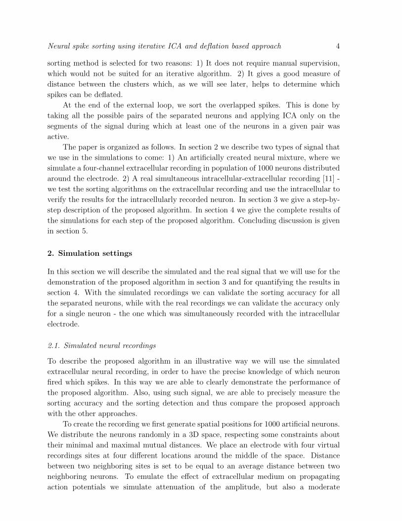
Neural spike sorting using iterative ICA and deflation based approach 4
sorting method is selected for two reasons: 1) It does not require manual supervision,
which would not be suited for an iterative algorithm. 2) It gives a good measure of
distance between the clusters which, as we will see later, helps to determine which
spikes can be deflated.
At the end of the external loop, we sort the overlapped spikes. This is done by
taking all the possible pairs of the separated neurons and applying ICA only on the
segments of the signal during which at least one of the neurons in a given pair was
active.
The paper is organized as follows. In section 2 we describe two types of signal that
we use in the simulations to come: 1) An artificially created neural mixture, where we
simulate a four-channel extracellular recording in population of 1000 neurons distributed
around the electrode. 2) A real simultaneous intracellular-extracellular recording [11] -
we test the sorting algorithms on the extracellular recording and use the intracellular to
verify the results for the intracellularly recorded neuron. In section 3 we give a step-by-
step description of the proposed algorithm. In section 4 we give the complete results of
the simulations for each step of the proposed algorithm. Concluding discussion is given
in section 5.
2. Simulation settings
In this section we will describe the simulated and the real signal that we will use for the
demonstration of the proposed algorithm in section 3 and for quantifying the results in
section 4. With the simulated recordings we can validate the sorting accuracy for all
the separated neurons, while with the real recordings we can validate the accuracy only
for a single neuron - the one which was simultaneously recorded with the intracellular
electrode.
2.1. Simulated neural recordings
To describe the proposed algorithm in an illustrative way we will use the simulated
extracellular neural recording, in order to have the precise knowledge of which neuron
fired which spikes. In this way we are able to clearly demonstrate the performance of
the proposed algorithm. Also, using such signal, we are able to precisely measure the
sorting accuracy and the sorting detection and thus compare the proposed approach
with the other approaches.
To create the recording we first generate spatial positions for 1000 artificial neurons.
We distribute the neurons randomly in a 3D space, respecting some constraints about
their minimal and maximal mutual distances. We place an electrode with four virtual
recordings sites at four different locations around the middle of the space. Distance
between two neighboring sites is set to be equal to an average distance between two
neighboring neurons. To emulate the effect of extracellular medium on propagating
action potentials we simulate attenuation of the amplitude, but also a moderate
Neural spike sorting using iterative ICA and deflation based approach 5
waveform smoothing which arises from a lowpass filtering properties of the medium [29].
We consider the smoothing between the recording sites to be negligible and simulate
only the smoothing which happens during the action potential propagation between
neurons and the electrode. We assume that the action potentials fired by the same
neuron are always recorded as spikes of the same shape. Moreover, since the smoothing
is generally moderate, we assume that the 1000 simulated neurons exhibit only 32
different spike shapes.. The 32 shapes are in fact templates generated by averaging
spikes coming from 32 different neurons, recorded by real extracellular recordings (the
recordings will be described in the next subsection). The length of each template is 60
samples, corresponding to 4ms real time. For each neuron we first generate a random
firing rate between 5Hz and 10Hz and then generate Poisson distributed firing times.
To make the simulated signal more realistic, we have to simulate the sampling
effects. Indeed, in real recordings spikes coming from a particular neuron generally
look different, because they are sampled at different time instants with respect to the
beginning of each spike. We simulate this effect by upsampling the spike templates by
a factor of 100. Then we associate the spike templates with the corresponding time
locations in the signal. Finally we subsample back to the original recording rate.
Assuming an isotropic setting, the extracellular potential typically decays as 1/rk,
where r is the Euclidian distance between the firing neuron and the recording site.
Depending on the position and orientation, the power k can take the value 1 (monopole
model, near the soma), 2 or higher (dipole model or multipole model, far-field). For sake
of simplicity, we consider k = 1 in our simulation. The first column on figure 2 shows
an example of the simulated recording obtained in this way. We refer to [30] and [31]
for further discussions on the propagation of action potentials through the extracellular
medium.
2.2. Real neural recording
A drawback of the validation using the simulated signal lies in the complexity of a real
neural mixture, which is very hard to reproduce artificially. Real recordings, depending
on the tissue in which the recording is taken, consist of superposed activity of up to
millions of neurons. The neurons interact through the large number of dendrites and
axons, what makes the spatial configuration extremely complex. Thus, the simulated
signal is often not a truthful counterpart of the real signal.
Apart from the simulated signal we examine the proposed algorithm using the real
neural recordings. We use the simultaneous intracellular-extracellular recordings from
a rat hippocampal area CA1 done by Henze et al., and described in [11]. When the
extracellular electrode is close to the intracellular, the activity of the neuron recorded
intracellularly will be also visible in the extracellular recording. Of course, with the
extracellular electrode activities of a vast number of neurons are recorded, so to separate
the activity of individual neurons we have to do spike sorting. Figure 1 shows a part
of such simultaneous recording. The four top plots show the extracellular recording

Neural spike sorting using iterative ICA and deflation based approach 6
with tetrode and the bottom plot shows the corresponding intracellular recording. The
action potentials fired by the neuron recorded intracellularly are clearly visible on all
four extracellularly recorded channels. This indicates that the recording sites are located
very close to each other.
0 2000 4000 6000 8000 10000
Cha
nnel
1
0 2000 4000 6000 8000 10000
Cha
nnel
2
0 2000 4000 6000 8000 10000
Cha
nnel
3
0 2000 4000 6000 8000 10000
Cha
nnel
4
0 2000 4000 6000 8000 10000
Intr
acel
lula
r
Samples
Figure 1. Simultaneous extracellular–intracellular recording. The four recording
sites are very close, so the action potentials recorded with the intracellular electrode
are clearly visible on all four extracellularly recorded channels.
On the plots of the extracellular channels we can also see the activity of other
neurons that are around the extracellular electrode. Notice that many spikes from the
other neurons have amplitudes similar to those of the spikes that come from the neuron
recorded intracellularly. Thus, the task of spike sorting is obviously not trivial in this
case.
3. The algorithm description
In this section we describe the proposed algorithm for multi-channel spike sorting.
The algorithm iteractively removes the activities of distant neurons from the original
recording as well as the activities of the neurons close to the electrode, once they are
separated from the mixture. By doing so we reduce the number of sources, which brings
the application of ICA in a more comfortable setting.
Apart from the recorded signal, to use the algorithm we only need to provide a
lower bound for the firing rate, call it G, and the spike detection threshold level. This

Neural spike sorting using iterative ICA and deflation based approach 7
lower bound is usually easy to set since, generally, we are not interested in separating
the activities of neurons that fired only a few spikes. A more detailed discussion on
how to chose G is given in our previous paper on spike sorting [23]. The choice of the
threshold level, on the other side, is not very critical, since we will simply neglect all the
spikes that belong to the cluster which has the lowest average peak-to-peak amplitude of
the spikes. This will make the algorithm more reliable, since the spikes with the lowest
amplitudes usually come from many different neurons, whose activity is only partially
detected.
We assume that a four-channel recording is given, but the algorithm is the same
for any number of channels. The four recorded signals are labeled as E1, E2, E3 and
E4. An example of a part of the simulated four-channel recording is shown on figure
2 and of the four-channel real recording on figure 3. Spikes from the neuron recorded
intracellularly are marked with the red stars.
Figure 2. 5000 samples from the simulated four-channel extracellular recording (first
column). 2D feature vector space with the extracted spikes - positive peak amplitude
vs negative peak amplitude (second column). Results of sorting algorithm from [23]
are given in the third column (only one cluster was detected for each channel).
To demonstrate that spike sorting is very difficult for such recording we apply
directly the greedy based spike sorting method described in [23]. First, we detect the
spikes using the spike detection method described in [9] and [32]. We then project

Neural spike sorting using iterative ICA and deflation based approach 8
Figure 3. 5000 samples from the real four-channel extracellular recording (first
column). 2D feature vector space with the extracted spikes - positive peak amplitude vs
negative peak amplitude (second column). Spikes that come from the neuron recorded
intracellularly are labeled with the red stars, while the rest of the spikes are labeled
with the blue dots. Results of sorting algorithm from [23] are given in the third column,
where the black dots marks are the detected centers of the clusters.
the spikes in a 2D vector space by keeping only two features per spike: the positive
and the negative peak amplitudes. Notice that one could also use, e.g., the two first
principal components. In the particular case, better (generally more reliable) results
were obtained when the positive and the negative peak amplitude were used as the
features, instead of the commonly applied PCA. The plots of the features are shown
next to the corresponding signals, in the second column on figures 2 and 3. In the third
column on figures 2 and 3 we give the outputs of the algorithm from [23]. The spikes
that are left unsorted by the algorithm are automatically eliminated and not plotted.
Note that the colors/symbols chosen for the representation of the clusters for the plots
in the second column are not related to the one in the third column. It is evident that
from such feature vector space it is not possible to do an accurate spike sorting.
We will now demonstrate the performance of the proposed algorithm using step-
by-step description. The flowchart that describes the proposed algorithm is shown on
figure 4.
• Step 1: ICA. We process the input signal with the FastICA algorithm described
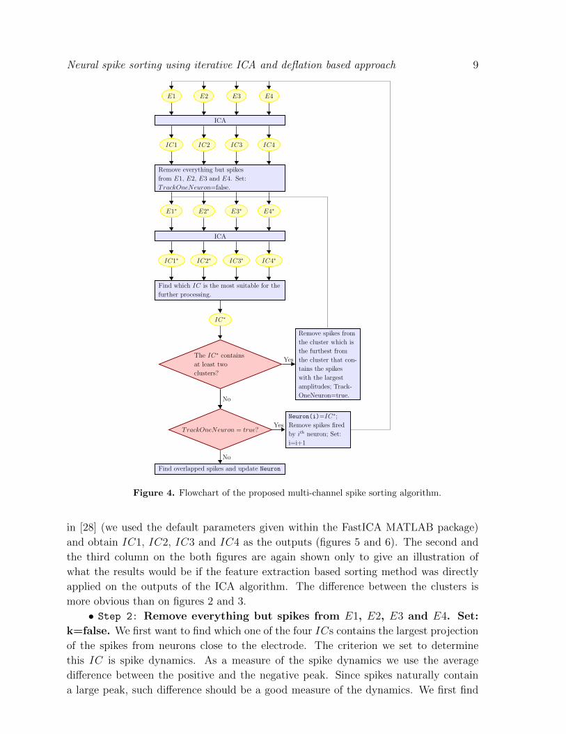
Neural spike sorting using iterative ICA and deflation based approach 9
ICA
E1 E2 E3 E4
Remove everything but spikes
from E1, E2, E3 and E4. Set:
TrackOneNeuron=false.
IC1 IC2 IC3 IC4
ICA
E1∗ E2∗ E3∗ E4∗
Find which IC is the most suitable for the
further processing.
IC1∗ IC2∗ IC3∗ IC4∗
IC∗
The IC∗ contains
at least two
clusters?
Remove spikes from
the cluster which is
the furthest from
the cluster that con-
tains the spikes
with the largest
amplitudes; Track-
OneNeuron=true.
Yes
TrackOneNeuron = true?
No
Neuron(i)=IC∗;
Remove spikes fired
by ith neuron; Set:
i=i+1
Yes
Find overlapped spikes and update Neuron
No
Figure 4. Flowchart of the proposed multi-channel spike sorting algorithm.
in [28] (we used the default parameters given within the FastICA MATLAB package)
and obtain IC1, IC2, IC3 and IC4 as the outputs (figures 5 and 6). The second and
the third column on the both figures are again shown only to give an illustration of
what the results would be if the feature extraction based sorting method was directly
applied on the outputs of the ICA algorithm. The difference between the clusters is
more obvious than on figures 2 and 3.
• Step 2: Remove everything but spikes from E1, E2, E3 and E4. Set:
k=false. We first want to find which one of the four ICs contains the largest projection
of the spikes from neurons close to the electrode. The criterion we set to determine
this IC is spike dynamics. As a measure of the spike dynamics we use the average
difference between the positive and the negative peak. Since spikes naturally contain
a large peak, such difference should be a good measure of the dynamics. We first find
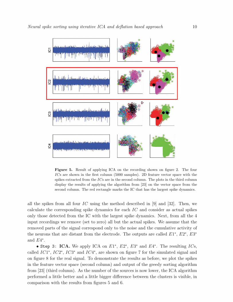
Neural spike sorting using iterative ICA and deflation based approach 10
Figure 5. Result of applying ICA on the recording shown on figure 2. The four
ICs are shown in the first column (5000 samples). 2D feature vector space with the
spikes extracted from the ICs are in the second column. The plots in the third column
display the results of applying the algorithm from [23] on the vector space from the
second column. The red rectangle marks the IC that has the largest spike dynamics.
all the spikes from all four IC using the method described in [9] and [32]. Then, we
calculate the corresponding spike dynamics for each IC and consider as actual spikes
only those detected from the IC with the largest spike dynamics. Next, from all the 4
input recordings we remove (set to zero) all but the actual spikes. We assume that the
removed parts of the signal correspond only to the noise and the cumulative activity of
the neurons that are distant from the electrode. The outputs are called E1∗, E2∗, E3∗
and E4∗.
• Step 3: ICA. We apply ICA on E1∗, E2∗, E3∗ and E4∗. The resulting ICs,
called IC1∗, IC2∗, IC3∗ and IC4∗, are shown on figure 7 for the simulated signal and
on figure 8 for the real signal. To demonstrate the results as before, we plot the spikes
in the feature vector space (second column) and output of the greedy sorting algorithm
from [23] (third column). As the number of the sources is now lower, the ICA algorithm
performed a little better and a little bigger difference between the clusters is visible, in
comparison with the results from figures 5 and 6.
Neural spike sorting using iterative ICA and deflation based approach 11
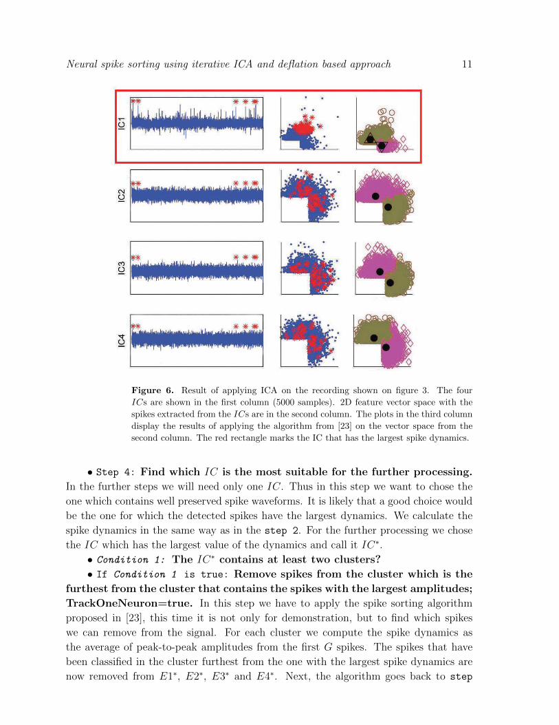
Figure 6. Result of applying ICA on the recording shown on figure 3. The four
ICs are shown in the first column (5000 samples). 2D feature vector space with the
spikes extracted from the ICs are in the second column. The plots in the third column
display the results of applying the algorithm from [23] on the vector space from the
second column. The red rectangle marks the IC that has the largest spike dynamics.
• Step 4: Find which IC is the most suitable for the further processing.
In the further steps we will need only one IC. Thus in this step we want to chose the
one which contains well preserved spike waveforms. It is likely that a good choice would
be the one for which the detected spikes have the largest dynamics. We calculate the
spike dynamics in the same way as in the step 2. For the further processing we chose
the IC which has the largest value of the dynamics and call it IC∗.
• Condition 1: The IC∗ contains at least two clusters?
• If Condition 1 is true: Remove spikes from the cluster which is the
furthest from the cluster that contains the spikes with the largest amplitudes;
TrackOneNeuron=true. In this step we have to apply the spike sorting algorithm
proposed in [23], this time it is not only for demonstration, but to find which spikes
we can remove from the signal. For each cluster we compute the spike dynamics as
the average of peak-to-peak amplitudes from the first G spikes. The spikes that have
been classified in the cluster furthest from the one with the largest spike dynamics are
now removed from E1∗, E2∗, E3∗ and E4∗. Next, the algorithm goes back to step
Neural spike sorting using iterative ICA and deflation based approach 12
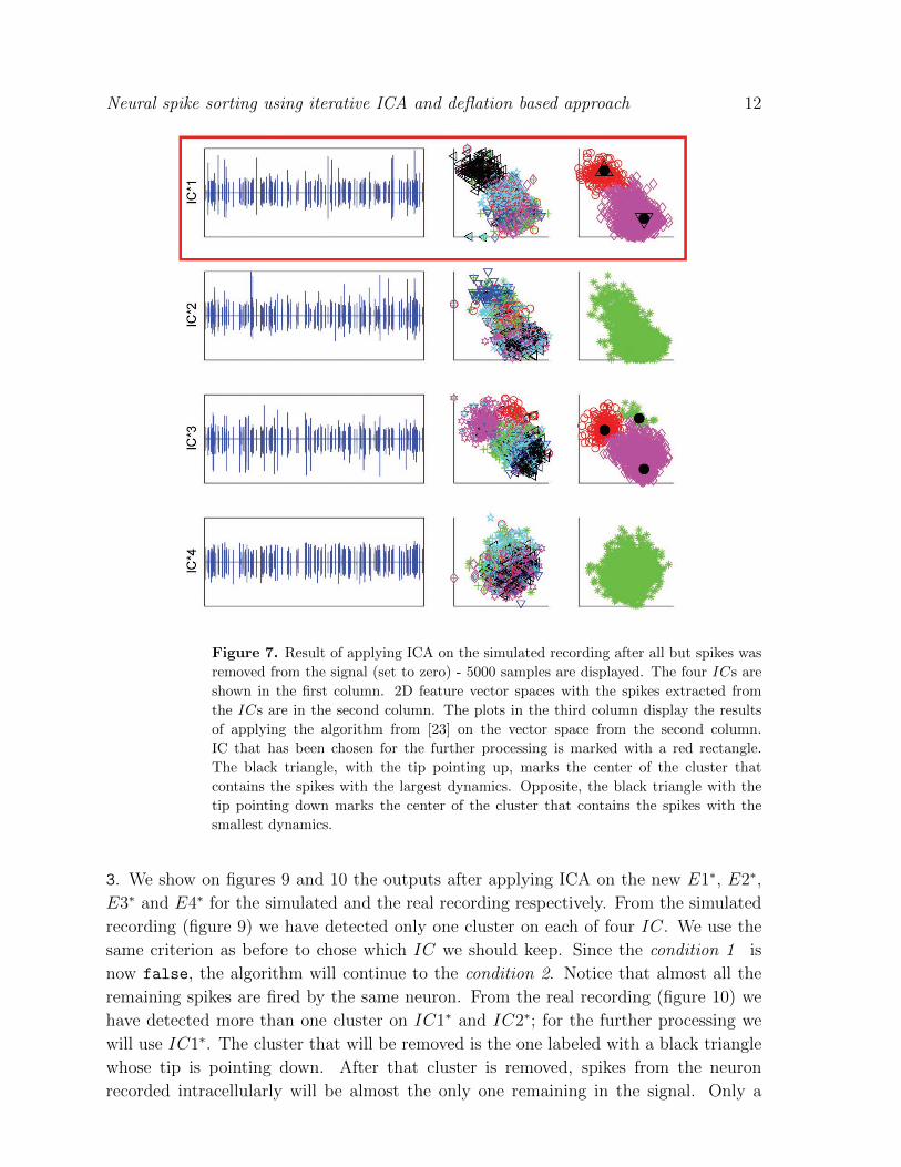
Figure 7. Result of applying ICA on the simulated recording after all but spikes was
removed from the signal (set to zero) - 5000 samples are displayed. The four ICs are
shown in the first column. 2D feature vector spaces with the spikes extracted from
the ICs are in the second column. The plots in the third column display the results
of applying the algorithm from [23] on the vector space from the second column.
IC that has been chosen for the further processing is marked with a red rectangle.
The black triangle, with the tip pointing up, marks the center of the cluster that
contains the spikes with the largest dynamics. Opposite, the black triangle with the
tip pointing down marks the center of the cluster that contains the spikes with the
smallest dynamics.
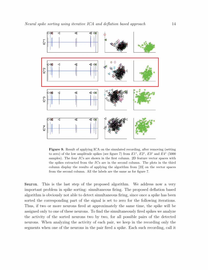
3. We show on figures 9 and 10 the outputs after applying ICA on the new E1∗, E2∗,
E3∗ and E4∗ for the simulated and the real recording respectively. From the simulated
recording (figure 9) we have detected only one cluster on each of four IC. We use the
same criterion as before to chose which IC we should keep. Since the condition 1 is
now false, the algorithm will continue to the condition 2. Notice that almost all the
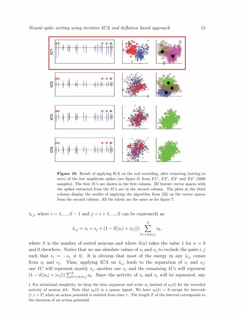
remaining spikes are fired by the same neuron. From the real recording (figure 10) we
have detected more than one cluster on IC1∗ and IC2∗; for the further processing we
will use IC1∗. The cluster that will be removed is the one labeled with a black triangle
whose tip is pointing down. After that cluster is removed, spikes from the neuron
recorded intracellularly will be almost the only one remaining in the signal. Only a

Neural spike sorting using iterative ICA and deflation based approach 13
Figure 8. Result of applying ICA on the real recording after all but spikes was
removed from the signal (set to zero) - 5000 samples are displayed. The four ICs are
shown in the first column. 2D feature vector spaces with the spikes extracted from
the ICs are in the second column. The plots in the third column display the results
of applying the algorithm from [23] on the vector space from the second column. All
the labels are the same as for figure 7.
few spikes from the intracellularly recorded neuron were removed. We set in this step
the flag TrackOneNeuron, in order to track if the algorithm converged just after a
new neuron is separated, what would indicate generally that no more neurons can be
separated from the given recording.
• If Condition 1 is false: Condition 2: TrackOneNeuron = true?
• If Condition 2 is true: Neuron(i)=IC∗; Remove the spikes fired by
the ith neuron; Set: i = i+ 1. If TrackOneNeuron is true that means that we have
detected more than one cluster in the previous iteration so now, since only one cluster is
left (the condition 1 was false), we assume that the remaining spikes are coming from
the same neuron. This is the ith separated neuron. To continue our iterative algorithm
we set to zero all the samples from the recording (from E1, E2, E3 and E4) when any
of the already detected neurons (Neuron(1), Neuron(2),...,Neuron(i)) was active and
go back to step 1. By doing this we removed an important high amplitude sources.
• If Condition 2 is false: Find the overlapped spikes and update
Neural spike sorting using iterative ICA and deflation based approach 14
Figure 9. Result of applying ICA on the simulated recording, after removing (setting
to zero) of the low amplitude spikes (see figure 7) from E1∗, E2∗, E3∗ and E4∗ (5000
samples). The four ICs are shown in the first column. 2D feature vector spaces with
the spikes extracted from the ICs are in the second column. The plots in the third
column display the results of applying the algorithm from [23] on the vector spaces
from the second column. All the labels are the same as for figure 7.
Neuron. This is the last step of the proposed algorithm. We address now a very
important problem in spike sorting: simultaneous firing. The proposed deflation based
algorithm is obviously not able to detect simultaneous firing, since once a spike has been
sorted the corresponding part of the signal is set to zero for the following iterations.
Thus, if two or more neurons fired at approximately the same time, the spike will be
assigned only to one of these neurons. To find the simultaneously fired spikes we analyze
the activity of the sorted neurons two by two, for all possible pairs of the detected
neurons. When analyzing the activity of each pair, we keep in the recording only the
segments when one of the neurons in the pair fired a spike. Each such recording, call it
Neural spike sorting using iterative ICA and deflation based approach 15
Figure 10. Result of applying ICA on the real recording, after removing (setting to
zero) of the low amplitude spikes (see figure 8) from E1∗, E2∗, E3∗ and E4∗ (5000
samples). The four ICs are shown in the first column. 2D feature vector spaces with
the spikes extracted from the ICs are in the second column. The plots in the third
column display the results of applying the algorithm from [23] on the vector spaces
from the second column. All the labels are the same as for figure 7.
si,j, where i = 1, ..., S − 1 and j = i+ 1, ..., S can be expressed‡ as:
si,j = si + sj + (1− δ(|si|+ |sj|))S∑
k=1,k 6=i,j
sk,
where S is the number of sorted neurons and where δ(u) takes the value 1 for u = 0
and 0 elsewhere. Notice that we use absolute values of si and sj to exclude the pairs i, j
such that si = −sj 6= 0. It is obvious that most of the energy in any si,j comes
from si and sj. Thus, applying ICA on si,j leads to the separation of si and sj:
one IC will represent mostly si, another one sj and the remaining ICs will represent
(1 − δ(|si| + |sj|))∑S
k=1,k 6=i,j sk. Since the activity of si and sj will be separated, any
‡ For notational simplicity, we drop the time argument and write sk instead of sk(t) for the recorded
activity of neuron #k. Note that sk(t) is a sparse signal: We have sk(t) = 0 except for intervals
[τ, τ +T ] when an action potential is emitted from time τ . The length T of the interval corresponds to
the duration of an action potential.

Neural spike sorting using iterative ICA and deflation based approach 16
spikes fired simultaneously by these two neurons should be visible on both of the ICs
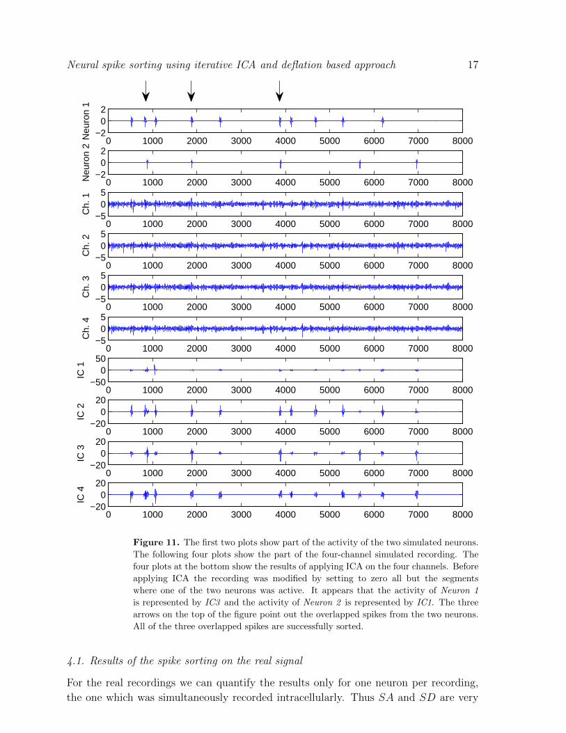
that represent the activity of these neurons. We demonstrate this by an example shown
in figure 11. In the first two rows we plot part of the activity of two simulated neurons
that fired three spikes simultaneously. The next four plots show four channels of the
simulated recording. The activity of the two neurons is visible, but hard to recognize,
especially to separate. We remove from the four channels everything but the segments
when any of the two neurons was active and apply ICA on such sparse signal. The
result of ICA is shown on four bottom plots on the same figure. Since this is the last
step of the proposed algorithm, we already have the estimation of the activity of all the
separated neurons. Thus, it is easy to find, from the result of ICA, that in this example
IC2 represents the activity of Neuron 1 and that IC3 represents the activity of Neuron
2. All the overlapped spikes are visible on both IC2 and IC3. They are now very easy
to localize and to update the detected activity of the separated neurons.
4. Results
We apply the algorithm described in the previous section on 5 real recordings and
on 10 simulated recordings. The results are given in tables 1 and 2. There are four
key-operations in the proposed algorithm: 1) removing of the noise (Noise rem.); 2)
removing of the spikes from the clusters far from the one that contains the spikes which
show the largest average peak-to-peak amplitude (Clus. rem.); 3) removing of the spikes
from already separated neurons (Sorted rem); 4) detection of the overlapped spikes
(Over. det.). We analyze contribution of each of these steps by simply comparing the
proposed algorithm to the algorithms which perform none, only one or more of these
steps. Namely, we compare the proposed algorithm with the following:
(i) Only the spike sorting algorithm, without performing ICA (Spike sor.).
(ii) ICA and spike sorting
(iii) ICA, spike sorting and removal of the spikes from already separated neurons.
(iv) As 3, but with removal of everything but spikes (step 2 of the algorithm).
(v) As 4, but with removal of clusters that generally contain spikes small in the
amplitude (clusters which are far from the one that contains the spikes which show
the largest average peak-to-peak amplitude).
The proposed algorithm is actually an extension of the algorithm (v), with a sequence
for the detection of the overlapped spikes.
We express the results through two parameters: 1) sorting accuracy (SA(%)) which
we define as ratio of accurately sorted spikes and total number of detected spikes and
2) sorting detection (SD(%)) which we define as ratio of accurately sorted spikes and
total number of spikes in the signal.
Neural spike sorting using iterative ICA and deflation based approach 17
0 1000 2000 3000 4000 5000 6000 7000 8000−2
02
Neu
ron
1
0 1000 2000 3000 4000 5000 6000 7000 8000−2
02
Neu
ron
2
0 1000 2000 3000 4000 5000 6000 7000 8000−5
05
Ch.
1
0 1000 2000 3000 4000 5000 6000 7000 8000−5
05
Ch.
2
0 1000 2000 3000 4000 5000 6000 7000 8000−5
05
Ch.
3
0 1000 2000 3000 4000 5000 6000 7000 8000−5
05
Ch.
4
0 1000 2000 3000 4000 5000 6000 7000 8000−50
050
IC 1
0 1000 2000 3000 4000 5000 6000 7000 8000−20
020
IC 2
0 1000 2000 3000 4000 5000 6000 7000 8000−20
020
IC 3
0 1000 2000 3000 4000 5000 6000 7000 8000−20
020
IC 4
Figure 11. The first two plots show part of the activity of the two simulated neurons.
The following four plots show the part of the four-channel simulated recording. The
four plots at the bottom show the results of applying ICA on the four channels. Before
applying ICA the recording was modified by setting to zero all but the segments
where one of the two neurons was active. It appears that the activity of Neuron 1
is represented by IC3 and the activity of Neuron 2 is represented by IC1. The three
arrows on the top of the figure point out the overlapped spikes from the two neurons.
All of the three overlapped spikes are successfully sorted.
4.1. Results of the spike sorting on the real signal
For the real recordings we can quantify the results only for one neuron per recording,
the one which was simultaneously recorded intracellularly. Thus SA and SD are very
Neural spike sorting using iterative ICA and deflation based approach 18
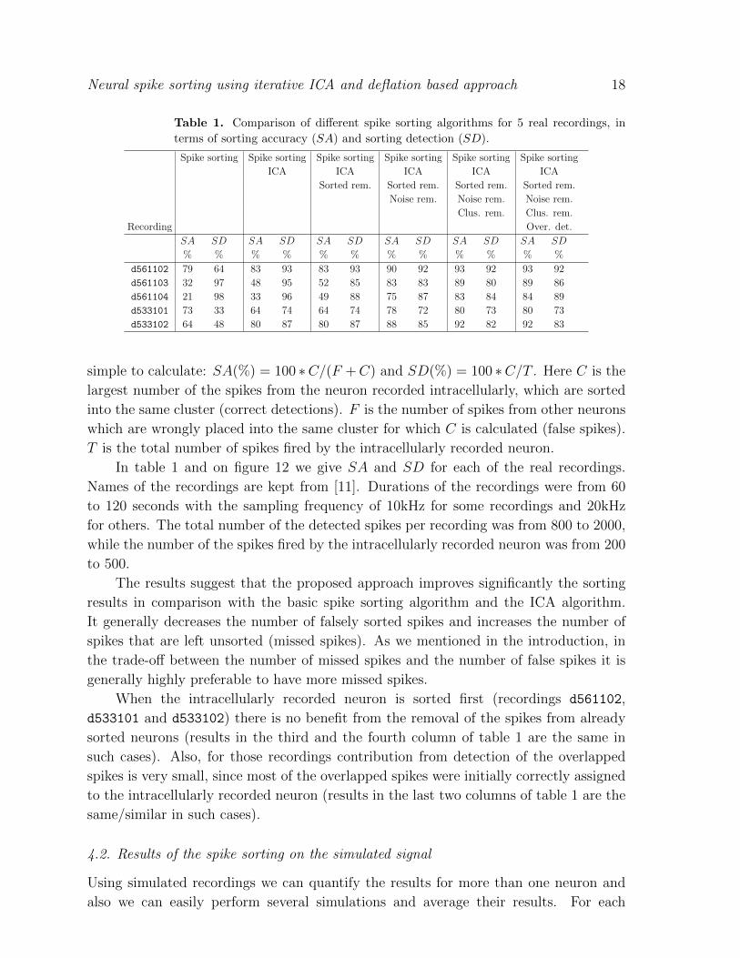
Table 1. Comparison of different spike sorting algorithms for 5 real recordings, in
terms of sorting accuracy (SA) and sorting detection (SD).
Spike sorting Spike sorting Spike sorting Spike sorting Spike sorting Spike sorting
ICA ICA ICA ICA ICA
Sorted rem. Sorted rem. Sorted rem. Sorted rem.
Noise rem. Noise rem. Noise rem.
Clus. rem. Clus. rem.
Recording Over. det.
SA SD SA SD SA SD SA SD SA SD SA SD
% % % % % % % % % % % %
d561102 79 64 83 93 83 93 90 92 93 92 93 92
d561103 32 97 48 95 52 85 83 83 89 80 89 86
d561104 21 98 33 96 49 88 75 87 83 84 84 89
d533101 73 33 64 74 64 74 78 72 80 73 80 73
d533102 64 48 80 87 80 87 88 85 92 82 92 83
simple to calculate: SA(%) = 100 ∗C/(F +C) and SD(%) = 100 ∗C/T . Here C is the
largest number of the spikes from the neuron recorded intracellularly, which are sorted
into the same cluster (correct detections). F is the number of spikes from other neurons
which are wrongly placed into the same cluster for which C is calculated (false spikes).
T is the total number of spikes fired by the intracellularly recorded neuron.
In table 1 and on figure 12 we give SA and SD for each of the real recordings.
Names of the recordings are kept from [11]. Durations of the recordings were from 60
to 120 seconds with the sampling frequency of 10kHz for some recordings and 20kHz
for others. The total number of the detected spikes per recording was from 800 to 2000,
while the number of the spikes fired by the intracellularly recorded neuron was from 200
to 500.
The results suggest that the proposed approach improves significantly the sorting
results in comparison with the basic spike sorting algorithm and the ICA algorithm.
It generally decreases the number of falsely sorted spikes and increases the number of
spikes that are left unsorted (missed spikes). As we mentioned in the introduction, in
the trade-off between the number of missed spikes and the number of false spikes it is
generally highly preferable to have more missed spikes.
When the intracellularly recorded neuron is sorted first (recordings d561102,
d533101 and d533102) there is no benefit from the removal of the spikes from already
sorted neurons (results in the third and the fourth column of table 1 are the same in
such cases). Also, for those recordings contribution from detection of the overlapped
spikes is very small, since most of the overlapped spikes were initially correctly assigned
to the intracellularly recorded neuron (results in the last two columns of table 1 are the
same/similar in such cases).
4.2. Results of the spike sorting on the simulated signal
Using simulated recordings we can quantify the results for more than one neuron and
also we can easily perform several simulations and average their results. For each
Neural spike sorting using iterative ICA and deflation based approach 19
Spike sorting + ICA + Sorted removed + Noise removed + Other clusters rem. + Detection of overlapped20
40
60
80
100
SA
(%)
Spike sorting + ICA + Sorted removed + Noise removed + Other clusters rem. + Detection of overlapped20
40
60
80
100
SD
(%)
Sorting method
recording: d561102 recording: d561103 recording: d561104 recording: d533101 recording: d533102
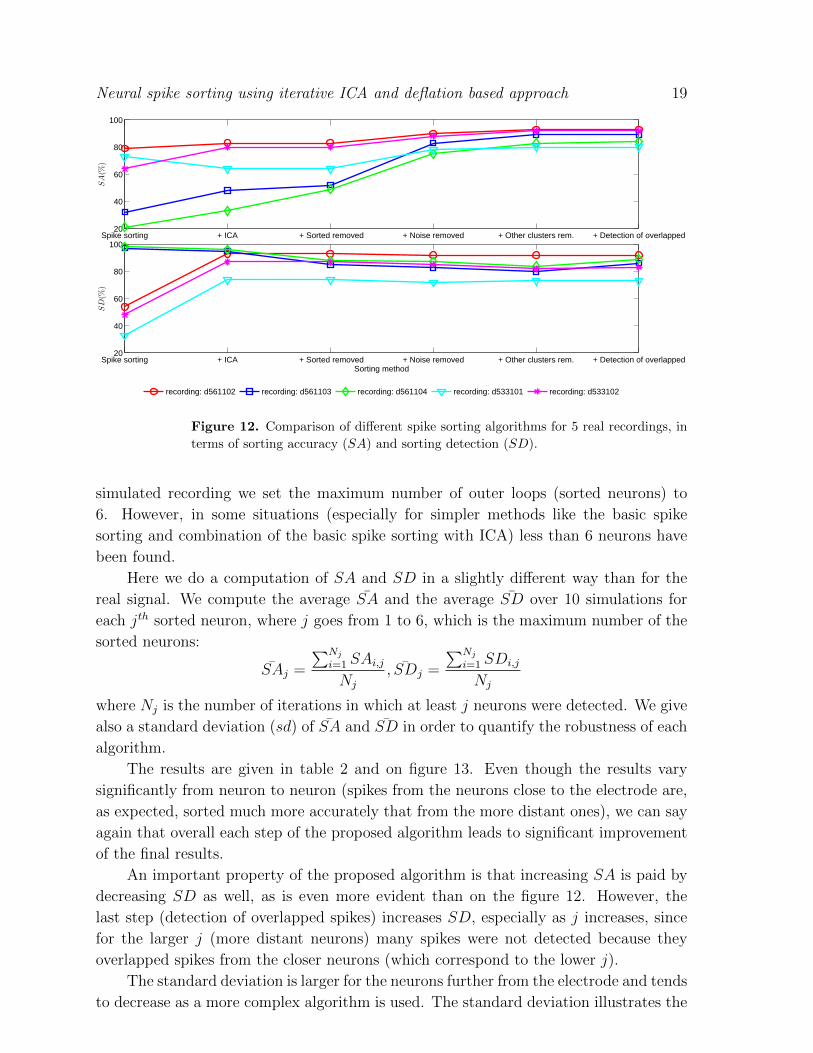
Figure 12. Comparison of different spike sorting algorithms for 5 real recordings, in
terms of sorting accuracy (SA) and sorting detection (SD).
simulated recording we set the maximum number of outer loops (sorted neurons) to
6. However, in some situations (especially for simpler methods like the basic spike
sorting and combination of the basic spike sorting with ICA) less than 6 neurons have
been found.
Here we do a computation of SA and SD in a slightly different way than for the
real signal. We compute the average SA and the average SD over 10 simulations for
each jth sorted neuron, where j goes from 1 to 6, which is the maximum number of the
sorted neurons:
SAj =
∑Nj
i=1 SAi,j
Nj
, SDj =
∑Nj
i=1 SDi,j
Nj
where Nj is the number of iterations in which at least j neurons were detected. We give
also a standard deviation (sd) of SA and SD in order to quantify the robustness of each
algorithm.
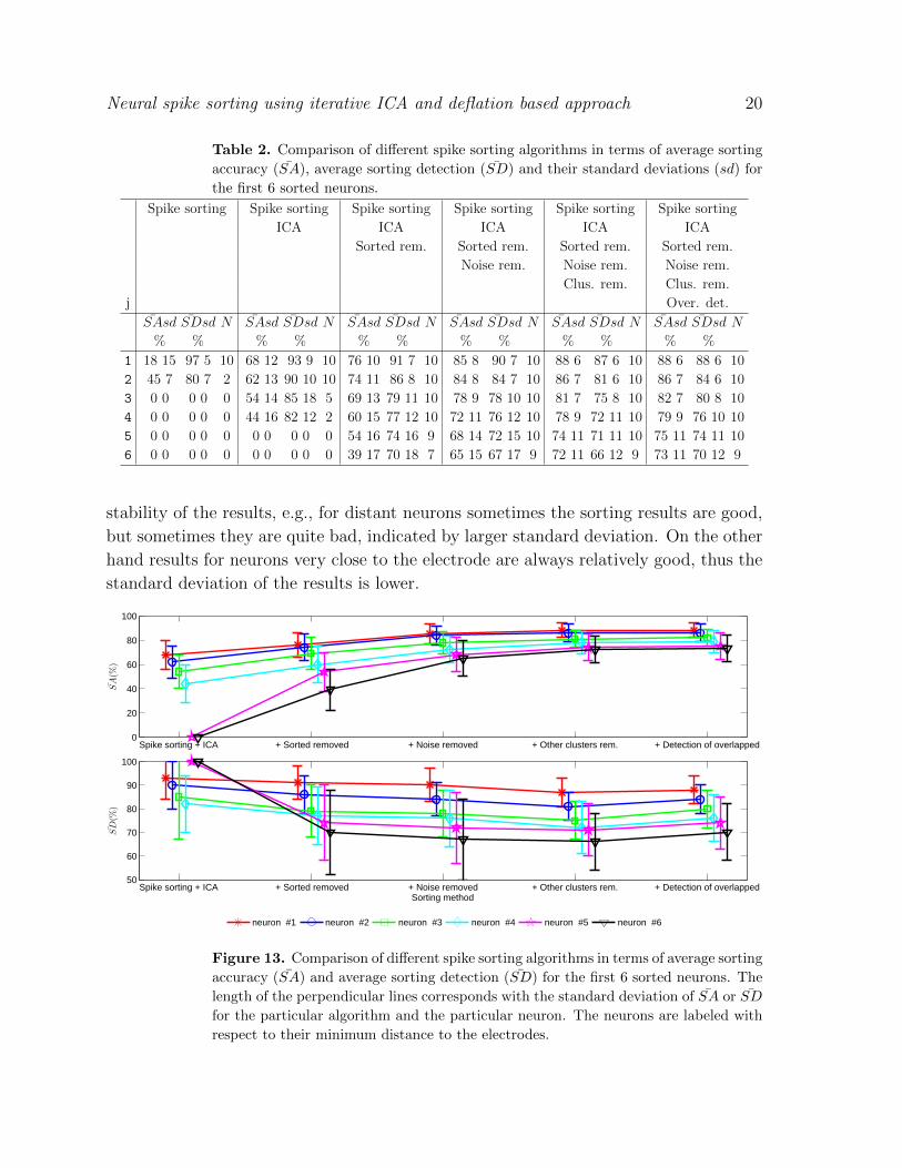
The results are given in table 2 and on figure 13. Even though the results vary
significantly from neuron to neuron (spikes from the neurons close to the electrode are,
as expected, sorted much more accurately that from the more distant ones), we can say
again that overall each step of the proposed algorithm leads to significant improvement
of the final results.
An important property of the proposed algorithm is that increasing SA is paid by
decreasing SD as well, as is even more evident than on the figure 12. However, the
last step (detection of overlapped spikes) increases SD, especially as j increases, since
for the larger j (more distant neurons) many spikes were not detected because they
overlapped spikes from the closer neurons (which correspond to the lower j).
The standard deviation is larger for the neurons further from the electrode and tends
to decrease as a more complex algorithm is used. The standard deviation illustrates the
Neural spike sorting using iterative ICA and deflation based approach 20
Table 2. Comparison of different spike sorting algorithms in terms of average sorting
accuracy (SA), average sorting detection (SD) and their standard deviations (sd) for
the first 6 sorted neurons.
Spike sorting Spike sorting Spike sorting Spike sorting Spike sorting Spike sorting
ICA ICA ICA ICA ICA
Sorted rem. Sorted rem. Sorted rem. Sorted rem.
Noise rem. Noise rem. Noise rem.
Clus. rem. Clus. rem.
j Over. det.
SAsd SDsd N SAsd SDsd N SAsd SDsd N SAsd SDsd N SAsd SDsd N SAsd SDsd N
% % % % % % % % % % % %
1 18 15 97 5 10 68 12 93 9 10 76 10 91 7 10 85 8 90 7 10 88 6 87 6 10 88 6 88 6 10
2 45 7 80 7 2 62 13 90 10 10 74 11 86 8 10 84 8 84 7 10 86 7 81 6 10 86 7 84 6 10
3 0 0 0 0 0 54 14 85 18 5 69 13 79 11 10 78 9 78 10 10 81 7 75 8 10 82 7 80 8 10
4 0 0 0 0 0 44 16 82 12 2 60 15 77 12 10 72 11 76 12 10 78 9 72 11 10 79 9 76 10 10
5 0 0 0 0 0 0 0 0 0 0 54 16 74 16 9 68 14 72 15 10 74 11 71 11 10 75 11 74 11 10
6 0 0 0 0 0 0 0 0 0 0 39 17 70 18 7 65 15 67 17 9 72 11 66 12 9 73 11 70 12 9
stability of the results, e.g., for distant neurons sometimes the sorting results are good,
but sometimes they are quite bad, indicated by larger standard deviation. On the other
hand results for neurons very close to the electrode are always relatively good, thus the
standard deviation of the results is lower.
Spike sorting + ICA + Sorted removed + Noise removed + Other clusters rem. + Detection of overlapped0
20
40
60
80
100
SA
(%)
Spike sorting + ICA + Sorted removed + Noise removed + Other clusters rem. + Detection of overlapped50
60
70
80
90
100
SD
(%)
Sorting method
neuron #1 neuron #2 neuron #3 neuron #4 neuron #5 neuron #6
Figure 13. Comparison of different spike sorting algorithms in terms of average sorting
accuracy (SA) and average sorting detection (SD) for the first 6 sorted neurons. The
length of the perpendicular lines corresponds with the standard deviation of SA or SD
for the particular algorithm and the particular neuron. The neurons are labeled with
respect to their minimum distance to the electrodes.
Neural spike sorting using iterative ICA and deflation based approach 21
5. Discussion
In this paper we proposed a new algorithm for spike sorting from multi-channel
recordings. We use iterative application of ICA and deflation to sort the spikes. Activity
at the recording sites is mutually highly dependant, while the activity of single neurons
is mutually much less dependant. This naturally suggests application of ICA to separate
the neural mixture.
A condition that the number of sensors should be equal or greater than the number
of sources appears as the major problem and limitation for application of ICA on neural
recordings. The proposed algorithm uses deflation to eliminate or at least to reduce the
contribution of different sources. In particular, we remove: 1) everything but spikes,
2) spikes which have already been sorted and 3) spikes which belong to the clusters far
from the one which contains the spikes of the largest average peak-to-peak amplitude.
Such deflation would result in inability of the algorithm to detect spikes fired by
different neurons at approximately the same time - simultaneous firing. Only one spike
per simultaneous firing could be detected. The solution to this problem is implemented
as the last step of the proposed algorithm. We take two of the separated neurons and
keep in the recording only the segments in which one of these two neurons was active.
Then we apply ICA on such sparse signal. Since we have only two high-energy sources
in the signal, ICA will, in most situations, be able to separate the activity of the two
neurons, including simultaneously fired spikes. We repeat this procedure for all the
possible pairs of the separated neurons.
The results given in tables 1 and 2 suggest that each step of the algorithm improves
the final sorting results. Overall, the algorithm significantly increases the number of
correctly sorted spikes while increasing the number of missed spikes by a relatively
small amount. ICA alone was not sufficient to obtain reliable results. It is important
to mention that if a recording is very noisy, the proposed algorithm will not be able to
detect any cluster.
In some particular cases, such as multi-electrode recordings from peripheral nerve
interfaces, the spike waveforms can arrive to the different recording sites with time delays
up to 0.1ms [33], [34]. FastICA algorithm is not adapted for such mixtures. In its present
form, the proposed algorithm is therefore not suitable for those cases. Nonetheless, the
proposed deflation methodology would still be useful if FastICA is replaced by some
convolutive version of ICA. In the convolutive case [35], [36], the recorded mixture is
described by an FIR filter model of the mixing process. Such model could be beneficial
in this particular case of spike sorting for two reasons: 1) Ability to account for different
delays of the source components; 2) Ability to account for echoes coming from different
parts of a nerve around the electrode.
As spike features we used simply positive and negative peak amplitude. However,
we could use practically any feature extraction method. Methods that can make the
difference between the spikes fired by different neurons more evident will of course lead
to better performance of the proposed algorithm, in terms of the number of sorted
Neural spike sorting using iterative ICA and deflation based approach 22
neurons and the sorting accuracy. Nevertheless, no matter how good the chosen feature
extraction technique is, the proposed algorithm should always improve the final sorting
results when they are compared to the results obtained with only ICA algorithm. Finally
we can say that the obtained results suggest that the proposed algorithm gives better
sorting results as compared to ICA.
Acknowledgments
This work was supported by the PHC COGITO project.
References
[1] J. D. Simeral, S. P Kim, M. J. Black, J. P. Donoghue, and L. R. Hochberg. Neural control of
cursor trajectory and click by a human with tetraplegia 1000 days after implant of an intracortical
microelectrode array. Journal of Neural Engineering, 8(2), April 2011.
[2] Cerebus Data Acquisition System - users manual. Blackrock Microsystems, 2009.
[3] M. S. Lewicki. A review of methods for spike sorting: the detection and classification of neural
action potentials. Network (Bristol, England), 9(4):53–78, November 1998.
[4] S. Gibson, J. W. Judy, and D. Markovic. Comparison of spike-sorting algorithms for future
hardware implementation. Annual Internationa Conference of the IEEE Engineering in
Medicine and Biology Society, 1:5015–20, 2008.
[5] E. N. Brown, R. E. Kass, and P. P. Mitra. Multiple neural spike train data analysis: state-of-the-
art and future challenges. Nature neuroscience, 7(5):456–461, May 2004.
[6] C. Pouzat, O. Mazor, and G. Laurent. Using noise signature to optimize spike-sorting and to assess
neuronal classification quality. Journal of Neuroscience Methods, 122(1):43–57, Dec 2002.
[7] K. H. Kim and S. J. Kim. Neural Spike Sorting Under Nearly 0-dB Signal-to-Noise Ratio Using
Nonlinear Energy Operator and Artificial Neural-Network Classifier. IEEE Transactions on
Biomedical Engineering, 47(10):1406–1411, Oct 2000.
[8] Z. Nenadic and J. W. Burdick. Spike detection using the continious wavelet transform. IEEE
Transactions in Biomededical Engineering, 52:74–87, 2005.
[9] Z. Tiganj and M. Mboup. Spike detection and sorting: Combining algebraic differentiations with
ica. In Independent Component Analysis and Signal Separation, 8th International Conference,
pages 475–482, Paraty, Brazil, 2009.
[10] N. G. Ilan and H. J. Don. Information theoretic bounds on neural prosthesis effectiveness: The
importance of spike sorting. In ICASSP, pages 5204–5207, 2008.
[11] D. A. Henze, Z. Borhegyi, J. Csicsvari, A. Mamiya, K. D. Harris, and G. Buzsaki. Intracellular
features predicted by extracellular recordings in the hippocampus in vivo. Journal of
Neurophysiology, 84(1):390–400, July 2000.
[12] D. A. Adamos, E. K. Kosmidis, and G. Theophilidis. Performance evaluation of PCA-based spike
sorting algorithms. Computer Methods and Programs in Biomedicine, 91:232–244, September
2008.
[13] R. Q. Quiroga, Z. Nadasdy, and Y. B. Shaul. Unsupervised spike detection and sorting with
wavelets and superparamagnetic clustering. Neural Computing, 16(8):1661–1687, August 2004.
[14] E. Hulata, R. Segev, and E. Ben-Jacob. A method for spike sorting and detection based on wavelet
packets and Shannon’s mutual information. Journal of neuroscience methods, 117(1):1–12, May
2002.
[15] Y. Ghanbari, L. Spence, and P. Papamichalis. A graph-Laplacian-based feature extraction
algorithm for neural spike sorting. In 31st Annual International Conference of the IEEE
Neural spike sorting using iterative ICA and deflation based approach 23
Engineering in Medicine and Biology Society, 3-6 Sept. 2009, pages 3142–5, Piscataway, NJ,
USA, 2009.
[16] E. Chah, V. Hok, A. Della-Chiesa, J. J. H. Miller, S. M. O’Mara, and R. B. Reilly. Automated
spike sorting algorithm based on Laplacian eigenmaps and k-means clustering. Journal of neural
engineering, 8(1), February 2011.
[17] S. Takahashi, Y. Anzai, and Y. Sakurai. A new approach to spike sorting for multi-neuronal
activities recorded with a tetrode–how ICA can be practical. Neuroscience research, 46(3):265–
272, July 2003.
[18] F. Wood, M. Fellows, J. Donoghue, and M. Black. Automatic spike sorting for neural decoding.
In Proceedings of the 26th Annual International Conference of the IEEE EMBS, volume 26 I,
pages 4009–4012, San Francisco, CA, USA, Sept. 2004.
[19] C. Vargas-Irwin and J. P. Donoghue. Automated spike sorting using density grid contour clustering
and subtractive waveform decomposition. Journal of neuroscience methods, 164(1):1–18, August
2007.
[20] J. S. Prentice, J. Homann, K. D. Simmons, G. Tkacik, V. Balasubramanian, and P. C. Nelson.
Fast, scalable, Bayesian spike identification for multi-electrode arrays. PLoS ONE, 6(7):e19884,
07 2011.
[21] D. Novak, J. Wild, T. Sieger, and R. Jech. Identifying number of neurons in extracellular recording.
In 4th Annual International Conference of the IEEE Engineering in Medicine and Biology Society
on Neural Engineering, pages 742–745, Antalya, Turkey, 2009.
[22] C. Fraley and A. E. Raftery. How many clusters? Which clustering method? Answers via model-
based cluster analysis. The Computer Journal, 41:578–588, 1998.
[23] Z. Tiganj and M. Mboup. A non-parametric method for automatic neural spikes clustering based
on the non-uniform distribution of the data. J. Neural Eng., 8(6):066014, 2011.
[24] Y. Shiraishi, N. Katayama, T. Takahashi, A. Karashima, and M. Nakao. Multi-neuron action
potentials recorded with tetrode are not instantaneous mixtures of single neuronal action
potentials. Annual International Conference of the IEEE Engineering in Medicine and Biology
Society., pages 4019–4022, 2009.
[25] G. D. Brown, S. Yamada, and T. J. Sejnowski. Independent component analysis at the neural
cocktail party. Trends in Neuroscience, 24(1):54–63, January 2001.
[26] S. Takahashi, Y. Anzai, and Y. Sakurai. Automatic sorting for multi-neuronal activity recorded
with tetrodes in the presence of overlapping spikes. Journal of neurophysiology, 89(4):2245–2258,
April 2003.
[27] P. Comon and C. Jutten. Handbook of Blind Source Separation, Independent Component Analysis
and Applications. Academic Press (Elsevier), 02 2010.
[28] A. Hyvarinen and E. Oja. Independent component analysis: algorithms and applications. Neural
Networks, 13(4-5):411–430, 06 2000.
[29] C. Bedard, H. Kroger, and A. Destexhe. Modeling extracellular field potentials and the Frequency-
Filtering properties of extracellular space. Biophysical Journal, 86(3):1829–1842, 2004.
[30] K. D. Harris, D. A. Henze, J. Csicsvari, H. Hirase, and G. Buzsaki. Accuracy of tetrode spike
separation as determined by simultaneous intracellular and extracellular measurements. Journal
of Neurophysiology, 84:401–414, Jul 2000.
[31] Pettersen K.H., Linden H., Dale A.M., and Einevoll G.T. Extracellular spikes and current-source
density. in Handbook of Neural Activity Measurement, edited by R. Brette and A. Destexhe,
Cambridge, 2012.
[32] M. Mboup. A Volterra filter for neuronal spike detection. Research report, INRIA, http://hal
inria fr/inria-00347048/en/, 2008.
[33] L. Citi, J. Carpaneto, K. Yoshida, K.P. Hoffmann, K.P. Koch, P. Dario, and S. Micera.
Characterization of tflife neural response for the control of a cybernetic hand. In Biomedical
Robotics and Biomechatronics, 2006. BioRob 2006. The First IEEE/RAS-EMBS International
Conference on, pages 477 –482, 2006.
Neural spike sorting using iterative ICA and deflation based approach 24
[34] Citi L., Carpaneto J., Yoshida K., Hoffmann K.P., Koch K.P., Dario P., and Micera S. On the use
of wavelet denoising and spike sorting techniques to process electroneurographic signals recorded
using intraneural electrodes. Journal of Neuroscience Methods, 172(2):294 – 302, 2008.
[35] J. Thomas, Y. Deville, and S. Hosseini. Time-domain fast fixed-point algorithms for convolutive
ICA. Signal Processing Letters, IEEE, 13(4):228 – 231, 2006.
[36] M. Dyrholm, S. Makeig, and L. K. Hansen. Model selection for convolutive ICA with an application
to spatio-temporal analysis of EEG. Neural Computation, 2006.